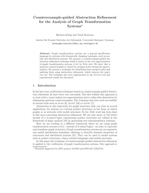
Counterexample-guided Abstraction Refinement for the Analysis of ...

Counterexample-guided Abstraction Refinementfor the Analysis of Graph TransformationSystems ⋆Barbara König and Vitali KoziouraInstitut für Formale Methoden der Informatik, Universität Stuttgart, Germany{koenigba,koziouvi}@fmi.uni-stuttgart.deAbstract. Graph transformation systems are a general specificationlanguage for systems with dynamically changing topologies, such as mobileand distributed systems. We propose a counterexample-guided abstractionrefinement technique which is based on the over-approximationof graph transformation systems (gts) by Petri nets. We show that aspurious counterexample is caused by merging nodes during the approximation.We present a technique for identifying these merged nodes andsplitting them using abstraction refinement, which removes the spuriousrun. The technique has been implemented in the Augur tool andexperimental results are discussed.1 IntroductionIn the last years verification techniques based on counterexample-guided abstractionrefinement [8] have been very successful. The idea behind this approach isto start with a coarse initial over-approximation and to refine this abstraction byeliminating spurious counterexamples. The technique has been used successfullyin several tools such as slam [6], blast [10] or magic [7].Abstraction is also important for graph structures that can arise in severalapplications, for instance as evolving pointer structures on the heap, as objectgraphs or as networks with mobile processes. So far, little work has been donein this area concerning abstraction refinement. We are only aware of [12] wheremodels of a 3-valued logics representing pointer structures are refined in theframework of shape analysis [16] by generating new instrumentation relations.Here we are working in a different framework where we are using graphtransformation systems (gts)—instead of 3-valued logics—in order to representand transform graph structures. Graph transformation systems are an expressiveand useful specification formalism, allowing to describe dynamic properties ofconcurrent and distributed systems [15]. They can be used to model systemssuch as pointer structures, object-oriented languages and mobile processes.In this paper the technique of counterexample-guided abstraction refinementis applied to the verification of graph transformation systems. Our approach is⋆ Research supported by DFG project SANDS and SFB 627 (NEXUS).

ased on a (partial order) technique that approximates gtss by Petri nets viaan unfolding construction [3]. More specifically, in this approach a finite overapproximationcalled Petri graph is constructed, which consists of a graph and aPetri net having the edges of the graph as places. The important property of theapproximation obtained in this way is that each graph reachable from the startgraph in the gts can be mapped, by merging some of its nodes, to a reachablemarking of the over-approximating Petri net. On the other hand there may besome markings reachable in the obtained Petri graph, which have no counterpartin the original gts. The sequence of events in the approximation leading to sucha graph is called a spurious run.In our case spurious runs are caused by the merging of graph nodes in theconstruction of the over-approximation. This is similar to the concept of summarynodes in shape analysis [16]. This paper describes how to construct a moreexact over-approximation by separating merged nodes for which these spuriousruns disappear. This procedure can be performed repeatedly for any number ofspurious runs.We believe that the technique of identifying the reason for the spurious runis independent of the abstraction mechanism used in this paper and could alsobe used in other frameworks dealing with approximations of graph structures.The techniques presented here are implemented as an extension of the toolAugur 1 . The experimental part of the paper compares this approach with analready existing abstraction refinement technique which reduces the number ofspurious examples by constructing an over-approximation which is exact up tosome pre-defined depth [5]. It is shown experimentally that counterexampleguidedabstraction refinement is faster and produces smaller Petri graphs.A long version of this paper is available as a technical report [11].2 Basic NotionsIn this section we describe the notions of hypergraph, gts, Petri net and Petrigraph and also show in an informal way how to construct over-approximatingPetri graphs.Definition 1 (hypergraphs and hypergraph morphisms). Let Λ be a setof labels where each label l ∈ Λ has an arity ar(l) ∈ N. A labelled hypergraphG is a tuple (V G ,E G ,c G ,l G ), where V G is a finite set of nodes, E G is a finiteset of edges, c G : E G → V ∗ G is a connection function and l G : E G → L is thelabeling function satisfying ar(l G (e)) = |c G (e)| for every e ∈ E G . The nodes arenot labelled.Let G and G ′ be two labelled hypergraphs. A hypergraph morphism (or simplymorphism) ϕ : G 1 → G 2 consists of a pair of total functions ϕ V : V G1 → V G2and ϕ E : E G1 → E G2 such that for every e ∈ E G1 it holds that l G1 (e) =l G2 (ϕ E (e)) and ϕ V (c G1 (e)) = c G2 (ϕ E (e)). A morphism is called edge-bijective1 Available from http://www.fmi.uni-stuttgart.de/szs/tools/augur/

(edge-injective) whenever it is bijective (injective) on edges. It is an isomorphismwhenever it is bijective on nodes and edges.Hypergraphs can be rewritten using rules of the following kind.Definition 2 (rewriting rule). A rewriting rule r is a triple (L,R,α), whereL and R are hypergraphs, called left-hand side and right-hand side respectivelyand α : V L → V R is an injective mapping, indicating how nodes are preserved.We demand that there are no isolated nodes in the left-hand side L and noisolated nodes in V R − α(V L ). Additionally E L must not be empty.The first condition says that we abstract from isolated nodes, whereas thesecond is a standard requirement for unfolding-based techniques, where everyrule must be consuming. Note furthermore that we do not consider rules thatpreserve edges of the left-hand side.For convenience we will in the following often assume that α is an inclusiondenoted by id, which can be enforced by renaming the nodes of the left or righthandside appropriately, and that the node and edge sets of L and R are disjointotherwise. That is, we demand that V L ⊆ V R and E L ∩ E R = ∅ which impliesthat the union L ∪ R is well-defined.Given a hypergraph, a rewriting rule and a match of the left-hand side, wecan apply this rule and replace the left-hand side by the right-hand side in thefollowing way. Additionally we define a partial morphism ν from the originalgraph to the rewritten graph, keeping track of preserved nodes and edges.Definition 3 (rewriting step). Let r = (L,R,id) be a rewriting rule. A matchof r in a hypergraph G is any morphism ϕ : L → G injective on edges. We canapply r to G according to the match ϕ and obtain a new graph H, written G ⇒ rH, which is defined as follows: V H = V G ⊎(V R −V L ), E H = (E G −ϕ(E L )) ⊎E Rand, defining ϕ:V R → V H by ϕ(v) = ϕ(v) if v ∈ V L and ϕ(v) = v otherwise, theconnection and labelling functions are given by c H (e) = c G (e), l H (e) = l G (e) ife ∈ E G − ϕ(E L ) and c H (e) = ϕ(c R (e)), l H (e) = l R (e) if e ∈ E R .We also define an injective partial morphism ν : G → H where ν V : V G → V Hand ν E : (E G − ϕ(E L )) → E H with ν(x) = x for every node or edge x.A graph transformation system (gts) G = (R,G 0 ) is a finite set of rulestogether with a start hypergraph (also called initial graph).Example: We illustrate the definitions of this chapter with an example describinga firewall system similar to the one introduced in [4]. This system contains an(arbitrarily large) set of processes running behind a firewall (safe processes) andone process in a public area (unsafe process). Any number of safe processes (SP)and connected locations (L) can be generated during runtime. The property toverify is that the unsafe process from the public area does not penetrate thefirewall. If this situation is detected, rule “Error” will be applied and an edgelabelled Error is created.Fig. 1 and Table 1 depict the initial graph and the rules of the firewall system.A double-headed arrow in a rule means that the rule can be applied in both

directions. Numbers close to the nodes indicate the mapping α. The private andpublic areas are connected by the firewall (F), and initially there is one unsafeprocesses (UP) in the public area. Only safe processes will be generated andthe firewall can be crossed in one direction only. Our aim is to show that noreachable graph contains the 0-ary edge Error.UPv 1Lw 1Fw 2Lv 2Fig. 1. Initial graph of the firewall system.Create ProcessSPSP/UPCross LocationSP/UPL1 2 1 2Cross ConnectionSP/UPSP/UPC1 2 1 2LLCCreate Connected LocationL1 2LC1 2LL1 2 1 2Cross FirewallSP/UPF1 2 1 2UPF1 2ErrorUPFFSP/UPError1 2Table 1. Rules of the firewall system.In order to approximate gtss we will employ Petri nets, which, as multisetrewriting systems, can be seen as a special case of graph rewriting. Petrinets are an easier model than gts and hence more amenable to analysis. Severalalgorithms and tools are available for their verification. Furthermore, byapproximating with Petri nets we will be able to preserve nice properties ofthe gts model, such as locality (state changes are only described locally) andconcurrency (no unnecessary interleaving of events) in the approximation.We will now introduce a notation for Petri nets. 22 By A ⊕ we denote a multiset over A and for a function f : A → B we denote byf ⊕ : A ⊕ → B ⊕ its extension to multisets. Furthermore for m ∈ A ⊕ and a ∈ A wedenote by m(a) the multiplicity of a in m.

Definition 4 (Petri net). Let ∆ be a finite set of labels. A ∆-labelled Petrinet is a tuple N = (S,T, • (),() • ,p), where S is the set of places, T is a set oftransitions, • (),() • : T → S ⊕ assign to each transition its pre-set and post-setand p : T → ∆ assigns a label to each transition. A marked Petri net is a pair(N,m N ), where N is a Petri net and m N ∈ S ⊕ is the initial marking.3 Approximated UnfoldingIn this section we will give a short overview of a technique that approximatesa graph transformation system by a structure that is both a Petri net and ahypergraph [3–5].First we define the notion of Petri graph which will be used to represent anover-approximation for a given gts. Note that the edges of the graph are at thesame time the places of the net and that the transitions are labelled with rulesof the gts.Definition 5 (Petri graph). Let G = (R,G 0 ) be a gts. A Petri graph (overR) is a tuple P = (G,N,µ), where G is a hypergraph, N = (E G ,T N , • (),() • ,p N )is an R-labelled Petri net where the places are the edges of G and µ associatesto each transition t ∈ T N , with p N (t) = (L,R,id), a hypergraph morphismµ(t) : L ∪ R → G such that • t = µ(t) ⊕ (E L ) and t • = µ(t) ⊕ (E R ).A Petri graph for the gts G is a pair (P,ι), where P = (G,N,µ) is a Petrigraph over R and ι : G 0 → G is a graph morphism. A marking is reachable(coverable) in Petri graph if it is reachable (coverable) in the underlying Petrinet with the multiset ι ⊕ (E G0 ) as the initial marking.We view Petri graphs as symbolic representations of transition systems withgraphs as states. Specifically each marking m of a Petri graph (G,N,m 0 ) canbe seen as representation of a graph, denoted by graph(m), according to thefollowing definition: We take the marked subgraph of G and duplicate each edgeas indicated by the marking.Alternatively one can define graph(m) as the unique graph H, up to isomorphism,such that H has no isolated nodes and there exists a morphismψ : H → G, injective on nodes, with ψ ⊕ (E H ) = m. Furthermore, wheneverthere exists a morphism ϕ : G ′ → G such that ϕ ⊕ (E G ′) ≤ m, then there existsan edge-injective morphism e m,ϕ :G ′ → graph(m) such that ψ ◦ e m,ϕ = ϕ.In order to obtain a Petri graph approximating a gts, we first need—asbuilding blocks—Petri graphs that describe the effect of a single rule.Definition 6 (Petri graph for a rewriting rule). Let r = (L,R,id) be arewriting rule. By P(t,r) = (G,N,µ) we denote a Petri graph with G = L∪R andN is a net with places S N = E L ∪ E R and one transition t such that p N (t) = r,• t = E L and t • = E R . Furthermore the morphism µ(t):L∪R → G is the identity.Given a gts G = (R,G 0 ) one can construct an over-approximating Petrigraph C G (also called the covering of G), using the following algorithm (see

[3]). It starts with a Petri graph P 0 that consists only of the start graph andcomputes C G iteratively. It is based on an unfolding technique which is combinedwith over-approximating folding steps which guarantee a finite approximation.Algorithm 7 (approximated unfolding) We set P 0 = (G 0 ,N 0 ,m 0 ), whereN 0 contains no transitions, m 0 = E G0 and let ι 0 :G 0 → G 0 be the identity. Aslong as one of the following steps is applicable, transform P i into P i+1 accordingto the possibilities given below (where folding steps take precedence overunfolding steps).Unfolding: Find a rule r = (L,R,id) ∈ R and a match ϕ : L → G i . Then choosea new transition t and extend P i by attaching P(t,r), i.e., take the disjoint unionof both Petri graphs and factor through the equivalence ≡ generated by e ≡ ϕ(e)for every e ∈ E L .Folding: Find a rule r = (L,R,id) ∈ R and two matches ϕ,ϕ ′ : L → G isuch that ϕ ⊕ (E L ) and ϕ ′⊕ (E L ) are coverable in N i and the second match iscausally dependent on the transition unfolding the first match. Then merge thetwo matches by setting ϕ(e) ≡ ϕ ′ (e) for each e ∈ E L and factoring through theresulting equivalence relation ≡.If neither possibility applies the Petri graph P i obtained in the last step isreturned. The result is denoted by C G . In [3] it has been shown that the algorithmalways terminates with a result unique up to isomorphism.In our running example, the constructed over-approximation consists of thehypergraph in Fig. 2 and the Petri net in Fig. 3. (Ignore the highlighted transitionsfor the moment.) Note that the set of edges of the graph correspondsexactly to the set of places of the net (the correspondence is indicated by givingindices to the labels).CSP 2UP 2v 1,2 L w 1,2SP 1UP 1FErrorFig. 2. Hypergraph component of the approximating Petri graph (firewall example).Before we can show in what way Petri graphs can be considered as abstractionsof gtss and before we discuss how they can be analyzed, we first need thedefinition of an abstract run of a gts and a notion of correspondence of twoabstract runs. Then we can define how Petri graphs can be seen as abstractionsof gtss.

Cross FirewallErrorErrorF SP 2LCrossFirewall CrossLocationCross LocationCreateProcessSP 1UP 2CrossConnectionCreateCreate LocationLocationCrossLocationC UP 1CrossLocationFig. 3. Petri net component of the approximating Petri graph (firewall example).Definition 8 (Abstract run). An abstract run of a gts (R,G 0 ) is a sequenceof hypergraphs J = (J 0 ⇛ r1 J 1 ⇛ r2 ... ⇛ rn J n ), where r i is a rule name,together with morphisms ϕ i : L i+1 → J i for each i = 1,...,n−1, where L i is theleft-hand side of rule r i ∈ R.Note that we do not demand that J i can be derived from J i−1 by applyingrule r i at match ϕ i . In this case J will be called a real run and we will also usethe symbol ⇒ instead of ⇛.Let J ′ = (J 0 ′ ⇛ r1 J 1 ′ ⇛ r2 ... ⇛ rn J n) ′ be another abstract run with morphismsϕ ′ i :L i+1 → J i ′ for each i = 1,...,n−1. We say that J ′ weakly correspondsto J (in symbols J ′ ≪ J ) if for each i = 1,...,n−1 there exist edgebijectivemorphism ξ i : J i ′ → J i for i = 0,...,n. If furthermore the followingdiagram commutes we say that J ′ corresponds to J and write J ′ ≪ J .ϕ ′ iL i+1J iϕ iJ ′ iξ iPetri graphs can, as mentioned above, be seen as symbolic representations ofgraph transition systems and also as representations of sets of abstract runs.Definition 9 (Abstract runs of a Petri graph). Let (P,ι) with P = (G,N,µ)be a Petri graph for a gts (R,G 0 ). Furthermore let m 0 [t 1 〉...[t n 〉m n be a firingsequence of the net N and let r i = p N (t i ) be the rules corresponding to thetransitions. We define morphisms ϕ i = e mi,µ(t i+1)| Li+1: L i+1 → graph(m i ),where L i+1 is the left-hand side of rule r i+1 . The sequence graph(m 0 ) ⇛ r1graph(m 1 ) ⇛ r2 ... ⇛ rn graph(m n ) together with the morphisms ϕ i is an abstractrun. We denote by Run A (P,ι) the set of all abstract runs of the Petrigraph (P,ι).Each real run J r = (G 0 ⇒ r1 G 1 ⇒ r2 ... ⇒ rn G n ) of the gts (R,G 0 ) can beconsidered as an abstract run where the ϕ i : L i+1 → G i represent the matchesof the left-hand sides of the rules r i .

Proposition 1. Let C G be an over-approximation for a gts G computed byAlgorithm 7. Then, for every real run J r of the graph transformation systemthere exists an abstract run J ∈ Run A (C G ) such that J r corresponds to J , i.e.,J r ≪ J .An abstract run J for which there does not exist a real run correspondingto J is called spurious. If, at the same time, it violates the property we attemptto verify, it is called a counterexample or error trace.We can now verify the gts by analyzing the Petri graph underlying the Petrinet. For instance, in order to show that no reachable graph contains a subgraphG s we add a new rule to the gts with G s as left-hand side and an edge witha new label Error in the right-hand side (see rule “Error” in Table 1). If wecan show that either no place labelled Error exists in the net or every suchplace is not coverable (this can be done using coverability graphs or backwardreachability algorithms [1]), then we can deduce that this property holds.However, if the approximation is too coarse, we might not be able to verifythe property. We have shown in [5] how to construct a sequence of subsequentlybetter unfolding—which however grow in size fairly rapidly—by forbidding foldingsteps up to depth k. Therefore we will now show how to successfully apply thetechnique of counterexample-guided abstraction refinement in our framework.4 Abstraction RefinementIn order to eliminate spurious runs, we will show that they are always causedby the fact that certain nodes were merged. We will identify these nodes andshow how to avoid their being merged in the next iteration, thereby avoidingthis particular spurious run and all other abstract runs corresponding to it ina sense made precise later. Merging of nodes is harmful since it might producenew left-hand sides, thereby leading to additional rewriting steps.4.1 Spurious RunsFor a given abstract run J = (graph(m 0 ) ⇛ r1 graph(m 1 ) ⇛ r2 ... ⇛ rngraph(m n )) of the Petri graph with morphisms ϕ i : L i+1 → graph(m i ) we defineH to be the set of real runs corresponding to the prefixes of J . Furthermore letH i be the set of hypergraphs reachable after i steps in a real run J r ∈ H. Itholds that H 0 = {G 0 }.An abstract run J is spurious if H n = ∅. If the run is spurious, there existsa k such that H k ≠ ∅, but H k+1 = ∅ (and therefore also H l = ∅ for l > k). It willbe shown in the following how to construct a new refined over-approximationC G ′ , which does not contain J and some other spurious runs corresponding to J .Example: We illustrate the idea of a spurious abstract run with the run correspondingto the firing of the highlighted transitions “Cross Location” and “Error”in Fig. 3. In fact, there is not real run in the original gts that correspondsto it.

4.2 Relations on Nodes for Refining Abstract RunsAccording to Algorithm 7 and Definition 8 it holds that H k ≠ ∅ and H k+1 = ∅if and only if for each G ∈ H k there exists no edge-injective morphism η :L k+1 → G such that the following diagram commutes, where ξ k is an edgebijectivemorphism derived from the correspondence property (see Definition 8).In other words: there is no way to find a match of the left-hand side in G thatagrees with the abstract run.L k+1ηG ξ k graph(m k )ϕ kFor if there were such a match morphism η, we could rewrite G to G ′ withrule r k+1 corresponding to the transition transforming m k to m k+1 . Because ofthe construction of the Petri graph, where the right-hand side of r i+1 has beenattached during an unfolding step, we would then be able to find an edge-bijectivemorphism ξ k+1 :G ′ → graph(m k+1 ) thus continuing the correspondence.Such a situation is only possible if ξ k is non-injective on some nodes of G,i.e., these nodes were merged during construction of the over-approximation C G ,which is the reason for the spurious run.Example: In our running example (see Fig. 1 and 2) the nodes v 1 and v 2 aswell as w 1 and w 2 of the initial hypergraph have been merged by the overapproximation,becoming v 1,2 and w 1,2 . This led to the spurious abstract rundescribed above.We will now show how to determine the node merges which caused the spuriousrun. Consider, for a fixed graph G and a morphism ξ k , the set Θ of possibleequivalence relations ∼ on nodes for a graph G ∈ H k such that, after mergingthe nodes in each equivalence class, we can find an appropriate match of theleft-hand side L k+1 in the graph G/ ∼ . More formally, we demand the existenceof an edge-injective morphism η ′ : L k+1 → G/ ∼ such that the following diagramcommutes, where ξ ′ k : G/ ∼ → graph(m k ) is obtained by quotienting ξ k accordingto ∼.L k+1η ′ ξ ′ kG/ ∼ graph(m k )ϕ kIn order to characterize the smallest equivalence in Θ consider a node v of theleft-hand side and determine a set Q v of nodes in G which have to be fused intoone node which is the image of v under η ′ . Let v ∈ V Lk+1 and let e be an edgeof L k+1 with 3 c i (e) = v for some i. For every edge e ′ in G with ξ k (e ′ ) = ϕ k (e)we require that c i (e ′ ) ∈ Q v .Consider the relation Q, where for each v ∈ V Lk+1 all nodes in Q v are relatedand the relation ̂Q which is the smallest equivalence containing Q.3 Note that by c i(e) we denote the i-the node in the sequence c(e).

Proposition 2. The equivalence ̂Q constructed above is the smallest equivalencecontained in Θ.Example: We consider again the abstract error trace J which can be obtainedby firing transitions “Cross Location” and “Error”. However, this error trace hasno real runs that correspond to it, which can be seen by computing the set Hof runs corresponding to prefixes of J . Here, the set H 0 consists of the initialhypergraph and the set H 1 contains one graph G 1 . The next rule “Error” cannotbe applied to G 1 in such a way that the corresponding diagram commutes andtherefore the set H 2 is empty.Fig. 4 shows the left-hand side of rule “Error”, G 1 ∈ H 1 and graph(m 1 ), thegraph corresponding to the marking reached after one step. One notices thatno appropriate morphism η can be found unless the nodes w 1 and w 2 in G 1are merged. Therefore we have Q w ′1= {w 1 ,w 2 }, Q w ′2= {w 2 } and the smallestequivalence relation ̂Q relates the nodes w 1 and w 2 and no other nodes. Notefor instance that w 2 must be contained in Q w ′1since both are attached to theunary edge labelled UP.left-hand side of rule ”Error”L 2UPFw ′ 1 w ′ 2η”real graph” G 1 graph(m 1 ) (graph generated by m 1 )UPL F Lv 1 w 1 w 2 v 2ξw 1,2UPLLv 1,2ϕFFig. 4. Hypergraphs G 1 ∈ H 1, L 2 and graph(m 1) from the firewall example.4.3 Elimination of Spurious RunsThe general idea for destroying spurious runs is to avoid the merging of nodesfrom the same equivalence class of ̂Q. For this reason we assign colours to thenodes of the graphs contained in H and disallow the merging of nodes correspondingto nodes with the same colour. For reasons that will become clearbelow a node may have several colours, i.e., a node v is associated to a set cols(v)of colours.For each G ∈ H k we and each morphism ξ k : G → graph(m k ) we considerthe corresponding relation Q G,ξk . Then we assign colours to nodes in such away that there exists at least one pair v 1 ,v 2 of nodes such that v 1 Q G,ξk v 2 andcols(v 1 ) ∩ cols(v 2 ) ≠ ∅. There are several ways to do this and all of them willhelp to eliminate the counterexample. In our implementation we choose a colorfor each set of nodes Q v and assign it to all nodes contained in Q v .In order to catch “bad” mergings as early as possible, these colours have tobe distributed to the remaining graphs contained in H. Let us recall here that

according to Definition 3 for each real run J r = (G 0 ⇒ r1 G 1 ... ⇒ rk G k ) fromH we have injective partial morphisms ν i : G i → G i+1 for i = 0,...,k−1. Usingthese partial morphisms we assign the colours of G k to the remaining graphs G icontained in H. We start from G k and proceed as follows: if a node v ∈ G i+1 hasa colour then we also assign this colour to the node ν −1 (v) if such a node exists.In this way a node may obtain several colours, due to the branching structureof the runs contained in H. We denote by cols(v) the set of colours of the nodev ∈ V Gj where G j ∈ H j .We are now ready to give the algorithm for computing the refined overapproximation.Algorithm 10 (Refined approximated unfolding)Input: A gts G, a set H of runs corresponding to prefixes of the counterexampleand a function cols assigning sets of colours to the nodes of the graphs in H.Output: The refined over-approximation C ′ G .We start constructing the new over-approximation C G ′ with the initial graphG 0 . Unfolding steps will be performed as described in Algorithm 7.For a folding step we disallow the merging of nodes corresponding to nodes inH having the same colour. More specifically, consider the over-approximation C G ′ ,which is currently being constructed. Now for each run J r = G 0 ⇛ r1 ... ⇛ rl G lin H where l < k check the following:We consider all abstract runs J = graph(m 0 ) ⇛ r1 ... ⇛ rl graph(m l ) of thecurrent Petri graph C G′ for which J r ≪ J and all edge-bijective morphismsξ:G i → graph(m i ) for i = 0,...,l. Whenever there are two nodes v 1 ,v 2 in G iwith cols(v 1 ) ∩ cols(v 2 ) ≠ ∅ and ξ(v 1 ) = ξ(v 2 ), we have erroneously merged twonodes in the approximation which should not have been merged. Consequentlythis folding step is undone.Previously rejected folding steps are recorded and are not any more consideredby the algorithm.In this way we will eliminate not only the spurious run but several more runswhich are characterized below (see Proposition 5).Example: Fig. 5 depicts the hypergraph obtained for the firewall example afterthe abstraction refinement procedure. As one can see, the “critical nodes” of thehypergraph, namely the nodes w 1 and w 2 , are now separated.4.4 CorrectnessIn the following we will show that Algorithm 10 terminates and that the refinedover-approximation is correct and more exact then the previous one.Let C G be an over-approximation with a spurious run J and let C G ′ be thecorresponding refined over-approximation. In [3] it is shown that the algorithmconstructing the over-approximating Petri graph terminates. We modified thealgorithm by forbidding some of the folding steps and hence we have to reprovetermination for the new version of the algorithm.

SPCv 1L F Lw 1 w v 22UPSP UP SP SPCFig. 5. Hypergraph obtained after abstraction refinement.Proposition 3. The algorithm computing the refined over-approximation C ′ G fora given gts G and a (spurious) abstract run J of C G terminates.Furthermore the new over-approximation is still a valid over-approximationas before.Proposition 4. Let C G ′ be the refined over-approximation of the gts. Then, forevery real run J r of the graph transformation system there exists an abstract runJ ∈ Run A (C G ′ ) such that J r corresponds to J , i.e., J r ≪ J .In the following two propositions we will show that we have eliminated thegiven spurious counterexample and have not added any new ones. First we shouldanswer the following question: what kind of runs have we eliminated by abstractionrefinement? It is easy to see that in the refined over-approximation we havelost the initial spurious counter-example J . In fact we have not only eliminatedJ , but some more runs as described below.Definition 11 (Correspondence with respect to runs). Let (P,ι) and(P ′ ,ι ′ ) be two Petri graphs for a gts (R,G 0 ). Furthermore let J ∈ Run A (P,ι)and J ′ ∈ Run A (P ′ ,ι ′ ) be two abstract runs of these Petri graphs and let H bethe set of real runs considered earlier. We say that J ′ corresponds to J withrespect to H if J ′ corresponds to J and a run J ′′ ∈ H of maximal length weaklycorresponds to a prefix of J ′ .Using this definition we can now state and prove the following propositions.Proposition 5. The refined over-approximation C G ′ , constructed above does notcontain any run J ′ corresponding to the spurious run J of C G with respect toH.We can also show that no new spurious runs have appeared, which meansthat the new approximation is strictly better than the old one.Proposition 6. If the refined over-approximation C G ′ contains a spurious runJ ′ , then it corresponds to some spurious run J in C G .We remark that the considered abstraction refinement approach can also beimplemented in the case of any number of spurious counterexamples by iterativelyrefining the abstraction. Naturally, due to undecidability and the factthat gtss are in general Turing-complete, there is no guarantee that it will everterminate.

5 Implementation and Experimental ResultsIn this section we consider examples of gtss and compare the experimentalresults obtained by refining the approximation by forbidding folding steps up toa certain depth (see [5]) and counterexample-guided abstraction refinement aspresented in this paper. It is shown that for practical purposes the new techniqueis usually more efficient.The algorithm was implemented in C++ under Linux and the computerparameters are 2*Xeon 2.4 GHz, 2 GB RAM.For case studies we have chosen two distributed systems: the running exampleof this paper (firewall example) and a system of public and private servers (fora description of the second example see [11]). If we compare the results in Tables2 and 3 it can be seen that in the case of counterexample-guided abstractionrefinement we have an advantage both in runtime for computing the approximationand in the size of the over-approximations, which are consequently easier toanalyze. The difference is especially pronounced for versions II, which use largerstart graphs.The efficiency of the abstraction refinement approach can be explained by thefact that we forbid to merge only those parts of the unfolding which are responsiblefor the spurious counterexample. This means that the over-approximationremains rather compact compared to the depth-based (or k-covering) approach,where we are not allowed to merge all items having depth smaller than k. Notethat for the firewall example it was not possible to verify the properties usingthe depth-based approached.examplek (depth) nodes edges transitions time (sec) verifiedPublic/private servers I 0 1 9 13 0.05 noPublic/private servers I 1 2 19 34 0.72 yesPublic/private servers II 0 1 10 14 0.05 noPublic/private servers II 1 1 11 16 0.07 noPublic/private servers II 2 3 31 63 7.16 yesFirewall I 0 2 8 13 0.05 noFirewall I 1 6 25 50 2.4 noFirewall I 2 10 51 148 138.18 noFirewall II 0 2 8 13 0.14 noFirewall II 1 8 39 82 13.7 noFirewall II 2 14 79 242 858.4 noTable 2. Verification results (abstraction refinement by forbidding folding steps up toa certain depth k, i.e., by computing k-coverings).

example nodes edges transitions time (sec) verifiedPublic/private servers I 2 16 25 0.67 yesPublic/private servers II 2 17 26 0.68 yesFirewall I 4 11 17 0.16 yesFirewall II 4 12 18 0.33 yesTable 3. Verification results (counterexample-guided abstraction refinement).6 ConclusionIn this paper we have shown how counterexample-guided abstraction refinementcan be applied to the analysis of dynamically evolving graphical structures ina fully automatic way. In this case we are not concerned with the abstractionof data values, but rather with graphs that are abstracted by merging nodesand edges, using the concept of graph morphisms. Hence, abstraction refinementcan in this case be described by exploiting commutativity or rather noncommutativityof morphisms as described in Section 4. Also, since we are dealingwith the approximation of graph structures rather than data values, no theoremprover is needed in order to determine the initial abstraction, instead we usetechniques for approximated unfolding developed in [3].Apart from smaller case studies we have used our approximated unfoldingtechnique to verify a mutual exclusion protocol [9] and to verify insertion ofelements into red-black trees [2]. We are currently working on an encoding ofsimple pointer programs into graph rewriting which will enable us to directlyverify operations on pointer structures.Research concerned with the verification of dynamically evolving graph structureswhich can be used to model distribution and mobility is fairly recent.There are contributions coming from the area of dataflow analysis such asshape analysis [16] as well as work directed more specifically towards the analysisof graph transformation systems [14, 13, 17, 9]. We believe that introducingcounterexample-based abstraction refinement is an important step in order tomake such verification techniques usable in practice. We also think that some ofthe techniques presented here can be employed in fairly general settings.Compared to shape analysis [16, 12] which is also concerned with over-approximationtechniques for graphical structures and which represents these structuresas models of a 3-valued logic, we follow a different approach where graphs arerepresented directly and graph morphisms are used as a convenient abstractionmechanism. Furthermore we approximate with Petri nets, which enable us to talkabout multiplicities of edges and can be conveniently analyzed using a varietyof existing Petri net tool.Acknowledgments: We would like to thank Tobias Heindel, Paolo Baldan andAndrea Corradini for many interesting discussions on the topics of this paper.

References1. P.A. Abdulla, B. Jonsson, M. Kindahl, and D. Peled. A general approach to partialorder reductions in symbolic verification. In Proc. of CAV ’98, pages 379–390.Springer, 1998. LNCS 1427.2. P. Baldan, A. Corradini, J. Esparza, T. Heindel, B. König, and V. Kozioura. Verifyingred-black trees. In Proc. of COSMICAH ’05, 2005. Proceedings available asreport RR-05-04 (Queen Mary, University of London).3. P. Baldan, A. Corradini, and B. König. A static analysis technique for graphtransformation systems. In Proc. of CONCUR ’01, pages 381–395. Springer, 2001.LNCS 2154.4. P. Baldan, A. Corradini, and B. König. Static analysis of distributed systems withmobility specified by graph grammars - a case study. In Proc. of IDPT ’02. Societyfor Design and Process Science, 2002.5. P. Baldan and B. König. Approximating the behaviour of graph transformationsystems. In Proc. of ICGT ’02, pages 14–29. Springer, 2002. LNCS 2505.6. T. Ball and S.K. Rajamani. Automatically validating temporal safety propertiesof interfaces. In Proc. of SPIN ’01, pages 103–122. Springer, 2001. LNCS 2057.7. S. Chaki, E. Clarke, A. Groce, S. Jha, and H. Veith. Modular verification ofsoftware components in C. In Proc. of ICSE ’03, pages 385–395. IEEE ComputerSociety, 2003.8. E. Clarke, S. Grumberg, S. Jha, Y. Lu, and H. Veith. Counterexample-guidedabstraction refinement. In Proc. of CAV ’00, pages 154–169. Springer, 2000. LNCS1855.9. F.L. Dotti, L. Foss, L. Ribeiro, and O. Marchi Santos. Verification of distributedobject-based systems. In Proc. of FMOODS ’03, pages 261–275. Springer, 2003.LNCS 2884.10. T.A. Henzinger, R. Jhala, R. Majumdar, and G. Sutre. Lazy abstraction. In Proc.of POPL ’02, pages 58–70. ACM, 2002.11. Barbara König and Vitali Kozioura. Counterexample-guided abstraction refinementfor the analysis of graph transformation systems. Technical Report 01/2006,Universität Stuttgart, 2006.12. A. Loginov, T. Reps, and M. Sagiv. Abstraction refinement via inductive learning.In Proc. of CAV ’05, pages 519–533. Springer, 2005. LNCS 3576.13. A. Rensink. Canonical graph shapes. In Proc. of ESOP ’04, pages 401–415.Springer, 2004. LNCS 2986.14. A. Rensink. State space abstraction using shape graphs. In Proc. of AVIS ’04,ENTCS, 2004. to appear.15. G. Rozenberg, editor. Handbook of Graph Grammars and Computing by GraphTransformation, Vol. 1: Foundations. World Scientific, 1997.16. M. Sagiv, T. Reps, and R. Wilhelm. Parametric shape analysis via 3-valued logic.TOPLAS, 24(3):217–298, 2002.17. D. Varró. Towards symbolic analysis of visual modeling languages. In Proc. ofGT-VMT ’02, volume 72 of ENTCS. Elsevier, 2002.