Counterexample-guided Abstraction Refinement for the Analysis of ...

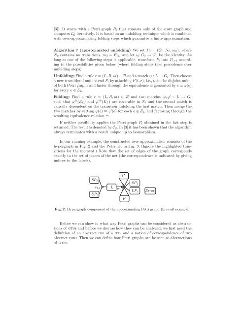
[3]). It starts with a Petri graph P 0 that consists only of the start graph andcomputes C G iteratively. It is based on an unfolding technique which is combinedwith over-approximating folding steps which guarantee a finite approximation.Algorithm 7 (approximated unfolding) We set P 0 = (G 0 ,N 0 ,m 0 ), whereN 0 contains no transitions, m 0 = E G0 and let ι 0 :G 0 → G 0 be the identity. Aslong as one of the following steps is applicable, transform P i into P i+1 accordingto the possibilities given below (where folding steps take precedence overunfolding steps).Unfolding: Find a rule r = (L,R,id) ∈ R and a match ϕ : L → G i . Then choosea new transition t and extend P i by attaching P(t,r), i.e., take the disjoint unionof both Petri graphs and factor through the equivalence ≡ generated by e ≡ ϕ(e)for every e ∈ E L .Folding: Find a rule r = (L,R,id) ∈ R and two matches ϕ,ϕ ′ : L → G isuch that ϕ ⊕ (E L ) and ϕ ′⊕ (E L ) are coverable in N i and the second match iscausally dependent on the transition unfolding the first match. Then merge thetwo matches by setting ϕ(e) ≡ ϕ ′ (e) for each e ∈ E L and factoring through theresulting equivalence relation ≡.If neither possibility applies the Petri graph P i obtained in the last step isreturned. The result is denoted by C G . In [3] it has been shown that the algorithmalways terminates with a result unique up to isomorphism.In our running example, the constructed over-approximation consists of thehypergraph in Fig. 2 and the Petri net in Fig. 3. (Ignore the highlighted transitionsfor the moment.) Note that the set of edges of the graph correspondsexactly to the set of places of the net (the correspondence is indicated by givingindices to the labels).CSP 2UP 2v 1,2 L w 1,2SP 1UP 1FErrorFig. 2. Hypergraph component of the approximating Petri graph (firewall example).Before we can show in what way Petri graphs can be considered as abstractionsof gtss and before we discuss how they can be analyzed, we first need thedefinition of an abstract run of a gts and a notion of correspondence of twoabstract runs. Then we can define how Petri graphs can be seen as abstractionsof gtss.