Real-time kinematic positioning with NASA's Internet-based ... - gdgps
Real-time kinematic positioning with NASA's Internet-based ... - gdgps
Real-time kinematic positioning with NASA's Internet-based ... - gdgps

You also want an ePaper? Increase the reach of your titles
YUMPU automatically turns print PDFs into web optimized ePapers that Google loves.
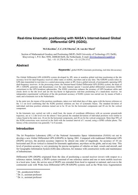
<strong>Real</strong>-<strong>time</strong> <strong>kinematic</strong> <strong>positioning</strong> <strong>with</strong> NASA’s <strong>Internet</strong>-<strong>based</strong> Global<br />
Differential GPS (IGDG).<br />
M.O.Kechine 1 , C.C.J.M.Tiberius 2 , H. van der Marel 3<br />
Section of Mathematical Geodesy and Positioning (MGP), Delft University of Technology (TU Delft),<br />
Kluyverweg 1, P.O. Box 5058, 2600GB Delft, the Netherlands. E-mail: M.O.Kechine@lr.tudelft.nl.<br />
Tel.: +31 15 278 8139; Fax: +31 15 278 3711.<br />
Abstract<br />
Keywords: global DGPS, <strong>kinematic</strong> <strong>positioning</strong>, real-<strong>time</strong> dm-accuracy<br />
The Global Differential GPS (GDGPS) system developed by JPL aims at seamless global real-<strong>time</strong> <strong>positioning</strong> at the dm<br />
accuracy level for dual-frequency receivers either static or mobile, anywhere and at any <strong>time</strong>. The GDGPS system relies on<br />
GPS data transmitted in real-<strong>time</strong> to a central processing center at JPL from a global network of permanently operating GPS<br />
dual-frequency receivers. At the processing center, the <strong>Internet</strong>-<strong>based</strong> Global Differential GPS (IGDG) system, the heart of<br />
JPL’s GDGPS, generates and disseminates over the open <strong>Internet</strong> special 1-second global differential corrections (IGDG<br />
corrections) to the GPS broadcast ephemerides. The IGDG corrections enhance the accuracy of GPS broadcast orbits and<br />
clocks down to the dm level and are the key-factor in high-precise real-<strong>time</strong> <strong>positioning</strong> of a stand-alone receiver. An<br />
independent experimental verification of the dm positional accuracy of IGDG system was carried out, by means of both a<br />
static and a <strong>kinematic</strong> test in the Netherlands.<br />
In the static test, the means of the position coordinates, taken over individual days of data, agree <strong>with</strong> the known reference at<br />
the 1-2 cm level confirming that the IGDG position solutions are free of systematic biases. The standard deviation of<br />
individual real-<strong>time</strong> position solutions turned out to be 10 cm for the horizontal components and 20 cm for the vertical<br />
component.<br />
In the <strong>kinematic</strong> test, carried out <strong>with</strong> a small boat, the means of coordinate differences <strong>with</strong> an accurate ground-truth<br />
trajectory, are at 1-2 dm level over the almost 3 hour period; the standard deviations of individual positions were similar to<br />
values found in the static test, 10 cm for the horizontal components, and 20 cm for the vertical component. More than 99% of<br />
the IGDG-corrections were received in the field <strong>with</strong> the nominal interval of 1 second, using a GPRS cellular phone. The<br />
latency of the corrections was generally 7 to 8 seconds.<br />
Introduction<br />
The Jet Propulsion Laboratory (JPL) of the National Aeronautics Space Administration (NASA) set out to<br />
develop a new Global Differential GPS (GDGPS) in Spring 2001. Compared <strong>with</strong> traditional Differential GPS<br />
(DGPS) services, the position accuracy improves by almost one order of magnitude. An accuracy of 10 cm<br />
horizontal and 20 cm vertical is claimed for <strong>kinematic</strong> applications, anywhere on the globe, and at any <strong>time</strong>. This<br />
level of position accuracy is very promising for precise navigation of vehicles on land, vessels and aircraft, and<br />
for Geographic Information System (GIS) data collection, for instance <strong>with</strong> construction works and maintenance<br />
of infrastructure.<br />
Differential GPS (DGPS) originated from the idea of <strong>positioning</strong> a second receiver (rover) <strong>with</strong> respect to a<br />
reference station. Initially, a DGPS system consisted of one reference station and one or more mobile receivers<br />
in a local area. Later, the service area of DGPS was extended from local to regional or national, and even to the<br />
continental scale <strong>with</strong> Wide-Area Differential GPS (WADGPS) systems such as the Wide-Area Augmentation<br />
1 Dr., postdoctoral fellow<br />
2 Dr. ir., assistant professor<br />
3 Dr. ir., assistant professor
System developed by U.S. Federal Aviation Administration, and the European Geostationary Navigation Overlay<br />
Service (EGNOS). GDGPS is regarded to be the further extension of Differential GPS to the global scale,<br />
capable of seamless <strong>positioning</strong> all over the world <strong>with</strong> dm positional accuracy. The most important feature of<br />
the GDGPS is a state-space approach, providing corrections to the GPS satellite orbits and clocks, but not to<br />
measurements, as in the traditional DGPS, see [1]. This guarantees global and uniform validity of the<br />
corrections.<br />
The <strong>Internet</strong>-<strong>based</strong> Global Differential GPS (IGDG) system produces and subsequently disseminates corrections<br />
to the broadcast ephemerides. IGDG can be considered as a realization of the concept of Precise Point<br />
Positioning (PPP), see [2]. Instead of <strong>positioning</strong> relative to a reference station or using a network, the idea was<br />
to take advantage of precise GPS satellite orbit and clock solutions for single receiver <strong>positioning</strong>. These<br />
products are the key to stand-alone precise <strong>positioning</strong> <strong>with</strong> eventually cen<strong>time</strong>ter-precision.<br />
An independent experimental verification of JPL’s IGDG has been carried out at the Delft University of<br />
Technology in the Netherlands, in cooperation <strong>with</strong> the Ministry of Transport, Public Works and Water<br />
Management, Geo-Information and ICT Department. The verification consisted of extensive stationary tests at a<br />
well-surveyed reference marker in Delft, and of a <strong>kinematic</strong> test using a small boat on a Dutch canal. The<br />
purpose of these tests was to verify, under practical circumstances, the real-<strong>time</strong> <strong>positioning</strong> accuracy of IGDG,<br />
as well as the availability and latency of the corrective information.<br />
After a description of the experimental set up, we will present in this paper <strong>positioning</strong> results and statistical<br />
analyses of both the static and <strong>kinematic</strong> test. Finally, we will demonstrate the results of a qualitative analysis of<br />
the IGDG differential corrections. The purpose was to ascertain the capability of the IGDG corrective<br />
information to improve the accuracy of the broadcast GPS orbits and clocks down to the decimeter level.<br />
1. <strong>Internet</strong>-<strong>based</strong> Global Differential GPS<br />
Precise satellite orbits and clocks at the global level are provided by the International GPS Service [3]. The IGS<br />
clocks and orbits are combinations of the individual solutions obtained by the different analysis centers and are<br />
very robust. IGS final orbit and clock solutions have a latency of 2 weeks, IGS rapid products of about 1 day,<br />
and ultra-rapid orbits are available twice each day. At present, the process of determination and dissemination of<br />
these products is moving towards near real-<strong>time</strong> execution. The availability of satellite orbit and clock solutions<br />
at decimeter accuracy, in real-<strong>time</strong>, enables Global Differential GPS.<br />
A subset of some 40 reference stations of <strong>NASA's</strong> Global GPS Network (GGN) allows for real-<strong>time</strong> streaming of<br />
data to a processing center, that determines and subsequently disseminates over the open <strong>Internet</strong>, in real-<strong>time</strong>,<br />
precise satellite orbits and clocks errors, as global differential corrections to the GPS broadcast ephemerides (as<br />
contained in the GPS navigation message). An introduction to IGDG can be found in [1] and [4]. Technical<br />
details are given in [5] and [6].<br />
<strong>Internet</strong>-<strong>based</strong> users can simply download the low-bandwidth correction data stream into a computer, where it<br />
will be combined <strong>with</strong> raw data from the user's GPS receiver. The final, but critical element in providing an endto-end<br />
<strong>positioning</strong> and orbit determination capability is the user's navigation software. In order to deliver 10 cm<br />
real-<strong>time</strong> <strong>positioning</strong> accuracy the software must employ most accurate models for the user's dynamics and the<br />
GPS measurements. For terrestrial applications these models include corrections for Earth tides, periodic<br />
relativity effect, and phase wind-up, see the review in [7]. The end-user version of the <strong>Real</strong>-Time Gipsy (RTG)<br />
software employs, in addition to these models, powerful estimation techniques for optimal <strong>positioning</strong> or orbit<br />
determination, including stochastic modelling, estimation of tropospheric delay, continuous phase smoothing and<br />
reduced dynamics estimation <strong>with</strong> stochastic attributes for every parameter.<br />
Results of static post-processing precise point <strong>positioning</strong> are shown in, for instance, the articles [7] and [8].<br />
Similarly, [9] evaluates JPL’s automated GPS data analysis service. Furthermore, <strong>kinematic</strong> post-processing<br />
point <strong>positioning</strong> results can be found e.g. in [10]. All the above examples, and also the results in the present<br />
contribution, rely on geodetic grade dual-frequency receivers.
2. Data processing<br />
In this paper we used GIPSY-OASIS II software, but not <strong>Real</strong>-Time Gipsy for the processing. Though the data<br />
of the tests were processed after data collection (post-processing), real-<strong>time</strong> operation was emulated. Epochs of<br />
data were processed sequentially and intermediate results (epoch after epoch) were used for the analysis.<br />
The GIPSY-OASIS II software, which stands for GPS Inferred Positioning System and Orbital Analysis and<br />
Simulation System [11], has been used for processing the data of both the static and <strong>kinematic</strong> experiment.<br />
Ionospheric-free combinations of dual-frequency GPS pseudorange code and carrier phase measurements were<br />
taken as basic observables. The whole set of parameters being determined <strong>with</strong> GIPSY consisted of the<br />
coordinates of the receiver’s antenna, phase ambiguities, receiver clock errors, wet zenith delays and troposphere<br />
gradients. The gradient parameters were included by default into the list of unknowns. However, as can be<br />
expected, for this kind of application it turned out not to be necessary to estimate gradients. The coordinates as<br />
well as the clock errors are modelled as white noise processes, phase ambiguities are considered as constant float<br />
numbers, and troposphere parameters are modelled as random walk <strong>with</strong> a random walk sigma of<br />
10.2mm / h for the wet zenith delays and of 0.3mm / h for the troposphere gradients (the GIPSY default<br />
values). The process noise for the coordinates of the receiver’s antenna was 1m in the static test, and 100 m in<br />
the <strong>kinematic</strong> test. The value of 100 m in the <strong>kinematic</strong> test was chosen in order to accommodate for dynamics of<br />
the boat and avoid possible divergence problems. By default a 15 degrees satellite elevation cut-off angle was<br />
used for data processing in the static test, and 10 degrees in the <strong>kinematic</strong> test.<br />
3. Static test<br />
During Autumn 2002, a geodetic dual-frequency receiver, an Ashtech Z-XII3 <strong>with</strong> a choke-ring antenna, was<br />
installed on a reference marker <strong>with</strong> accurately known position coordinates, see figure 1.<br />
Figure 1: The Ashtech choke-ring antenna, <strong>with</strong> conical radome, installed on the observation platform of the<br />
(formerly) TU Delft building for Geodesy, for the static test. This site, about 30 meters above ground level,<br />
offers unobstructed visibility of the sky, down to the horizon. The satellite elevation cut-off angle was<br />
maintained at 10 degrees during the measurements (elevation cut-off angle for the data processing was 15<br />
degrees).<br />
Continuous GPS measurements are carried out, on a neighbouring marker at this site, and these data are being<br />
used on a weekly basis as a part of the EUREF Permanent Network (EPN) [12]. The position of this marker is<br />
well known in ITRF2000. The local tie to the marker used for the static test is accurately known from earlier<br />
surveys and were independently verified for this test. Thereby, accurate reference coordinates in ITRF2000, at<br />
the epoch of observation, were available for the static test.<br />
Data were collected for five consecutive days at a 1 second interval. All 5 × 24 hours were processed in batches<br />
of 3 hours (the filter was restarted each 3 hours <strong>with</strong> the next data file) using JPL’s GIPSY software, in <strong>kinematic</strong><br />
mode, though the receiver was actually stationary. For the static test computations, the wet troposphere was<br />
estimated as a constant parameter over a 3-hour <strong>time</strong> span (one parameter per each batch); the troposphere
gradients were estimated stochastically <strong>with</strong> a (small) random walk sigma of 0.3mm / h . At the same <strong>time</strong>, as<br />
additional experiments showed, exclusion of the troposphere gradients from the list of unknown (stochastic)<br />
parameters did not change significantly the results of the Ashtech antenna <strong>kinematic</strong> <strong>positioning</strong>.<br />
Accuracy<br />
Table 1 demonstrates the mean and standard deviation of the position differences <strong>with</strong> the known reference at 1<br />
second interval, on all five days. The means of the position coordinates taken over each <strong>time</strong> one day of data do<br />
agree <strong>with</strong> the known reference at the 1-2 cm level in ITRF2000. The IGDG position solutions appeared to be<br />
really free of systematic biases. The standard deviations of individual real-<strong>time</strong> position solutions turned out to<br />
be 10 cm for the horizontal components and 20 cm for the vertical component. This agrees <strong>with</strong> earlier claims on<br />
IGDG position accuracy.<br />
day North East Height<br />
mean stdev mean stdev mean stdev<br />
1 1.7 10.1 -1.7 10.4 -0.5 21.4<br />
2 -0.4 8.8 0.7 8.1 -5.5 16.2<br />
3 -2.0 9.5 1.1 7.0 -0.8 19.1<br />
4 2.9 12.9 -1.3 11.0 -0.8 22.7<br />
5 0.9 8.7 0.4 6.7 0.7 18.6<br />
Table 1: Mean and standard deviation of position differences, in cen<strong>time</strong>ter, in static test.<br />
During the day, the number of satellites above the 15 degrees elevation cut-off angle was usually in the range<br />
from 5 through 8; there were a few periods <strong>with</strong> only the minimum of 4 satellites. Over the day, two periods<br />
occurred <strong>with</strong> only 4 satellites for which the PDOP exceeded the value of 10. In these cases the standard<br />
deviation values rose up to 40-50 cm, in particular for the vertical. Also, it was found that frequent changes in the<br />
satellite configuration (satellites disappearing, new satellites showing up) may lead to deteriorated <strong>positioning</strong><br />
performance.<br />
Because we started the filtering process for every 3-hour data batch <strong>with</strong> the same position uncertainty and initial<br />
receiver position, the Kalman filter required some <strong>time</strong> to ‘stabilize’ the position estimates. This circumstance<br />
was used to evaluate the filter convergence <strong>time</strong> in the static test. Analyses of the <strong>positioning</strong> results showed that<br />
almost complete convergence was reached in the first few seconds after the initial epochs, even if deviations of<br />
the position estimates were large in magnitude (the deviations exceeded the 1-m level at maximum).<br />
Final orbit and clock products<br />
Though only real-<strong>time</strong> satellite orbit and clock products are relevant to navigation applications, comparison of<br />
the <strong>positioning</strong> results <strong>with</strong> those obtained on the basis of final orbit and clock products, gives a first impression<br />
of the quality of the real-<strong>time</strong> products. The data of day 4 and 5 of the static test were used, and a 5 minutes<br />
sampling interval was taken, in order to basically avoid interpolation effects (<strong>with</strong> the orbits and clocks). Table 2<br />
gives the standard deviations of the coordinate differences, in North, East and Height. Avoiding interpolation<br />
effects (columns real-<strong>time</strong>) causes a factor of 2 reduction in the standard deviation (cf. table 1), and using the<br />
final products (three columns at right) yields again a factor 2 of improvement.<br />
real-<strong>time</strong> final<br />
day North East Height North East Height<br />
4 5.4 5.2 9.0 3.0 2.9 4.8<br />
5 4.6 4.6 8.7 2.6 2.9 4.2<br />
Table 2: Standard deviation of position differences at 5 minutes interval, in cen<strong>time</strong>ter, in static test, using real<strong>time</strong><br />
orbits and clocks at left, and using final orbits and clocks at right.<br />
4. Kinematic test<br />
The <strong>kinematic</strong> test was carried out during Spring 2003. With a small boat, see figure 2, a 2 km stretch on the<br />
Schie-canal was sailed repeatedly. A dual-frequency Ashtech Z-XII3 receiver, connected to an Ashtech chokering<br />
antenna, was used on the boat for the <strong>kinematic</strong> test. A trajectory of almost 3 hours was observed, again at a
1 second interval. There were 8 to 10 satellites above the 10 degrees elevation cut-off angle and these were<br />
consequently used in the position solution (apart from two short periods <strong>with</strong> 7 satellites).<br />
For the purpose of computing an accurate reference trajectory for the on-board receiver, the site and equipment<br />
of the static test served as a local reference station (about 3-5 km away). In-house software was used to compute<br />
the dual frequency carrier phase, ambiguity fixed, solution, using the data of both the stationary reference and the<br />
rover on the boat in a classical short-baseline model. The resulting trajectory in ITRF2000 at the epoch of<br />
observation, possesses cm accuracy, and is thereby one order of magnitude more accurate than the IGDG<br />
solution, consequently serving as the ground-truth.<br />
Figure 2: The boat used for the <strong>kinematic</strong> test on the Schie-canal between Delft and Rotterdam in the<br />
Netherlands.<br />
Position accuracy<br />
Differences, in North, East and Height, of the filtered position estimates for the Ashtech receiver on the boat <strong>with</strong><br />
the ground-truth trajectory are shown in figure 3. One can note a peak in the Height component, between 9:40<br />
and 9:50. The peak is most likely caused by a deviating clock error estimate for one of the satellites in the JPL<br />
real-<strong>time</strong> ephemerides at epoch 9:45. Additional tests showed that removing GPS measurements throughout the<br />
10-min <strong>time</strong> span between 9:40 and 9:50 for SVN15 had a major impact on the behaviour of the Height<br />
component, the deviation was reduced by approximately a factor 2.<br />
Table 3 gives the mean and standard deviation of the position differences in the <strong>kinematic</strong> test. Both the full<br />
period is considered, as well as the period <strong>with</strong>out the ‘initialization’, leaving out the first 40 minutes.<br />
Examination of table 3 shows that, apart from the initialization, the standard deviations (the data sample<br />
scattering around the mean) are again 10 cm for the horizontal components and 20 cm for the vertical, but the<br />
filtered position estimates in the <strong>kinematic</strong> test appeared to be slightly biased; the means over the full test period<br />
are at 1-2 dm level.<br />
North East Height<br />
mean stdev mean stdev mean stdev<br />
full -5.0 19.1 13.3 18.9 -17.2 59.4<br />
w/o init -2.2 8.0 18.9 12.3 -24.7 20.3<br />
Table 3: Mean and standard deviation of position differences, in cen<strong>time</strong>ter, in <strong>kinematic</strong> test.<br />
Effect of weakened satellite geometry<br />
Because of good environment in the area of the <strong>kinematic</strong> experiment (open field, no big trees and man-made<br />
constructions nearby the channel), the visibility was quite good, and up to 10 satellites were observed<br />
simultaneously in the sky above the elevation cut-off angle of 10 degrees. As a result, we have a quite stable and<br />
strong satellite-to-user geometry (PDOP was about 2). We assessed the influence of a weakened satellite<br />
geometry on the <strong>kinematic</strong> <strong>positioning</strong> results by setting the minimal elevation angle to 15 degrees instead of 10<br />
degrees. The accuracy estimates are given in table 4.
North East Height<br />
mean stdev mean stdev mean stdev<br />
full -0.7 28.6 17.6 15.7 -20.4 64.9<br />
w/o init 0.0 9.8 21.2 13.3 -22.4 32.3<br />
Table 4: Mean and standard deviation of position differences, in cen<strong>time</strong>ter, in <strong>kinematic</strong> test. Satellite cut-off<br />
elevation angle is 15 degrees.<br />
As expected, augmentation of the minimal elevation angle weakens the satellite geometry. This immediately led<br />
to some degradation of the accuracy of the boat position estimates (cf. table 3).<br />
Figure 3: Coordinate <strong>time</strong> series for the receiver<br />
onboard the boat in the <strong>kinematic</strong> test<br />
corresponding to strategy B from table 5.<br />
Figure 4: Coordinate <strong>time</strong> series for the receiver<br />
onboard the boat in the <strong>kinematic</strong> test<br />
corresponding to strategy A from table 5.<br />
5. Effect of troposphere estimation on the <strong>kinematic</strong> <strong>positioning</strong><br />
The GIPSY-OASIS II software is able to estimate both the wet troposphere (zenith wet delays) and the<br />
troposphere gradients. These parameters are modelled as either constant (bias) parameters over a whole<br />
observation <strong>time</strong> span or stochastic parameters driven by a random process noise. Additional investigations have<br />
been made on the PPP processing strategy for <strong>kinematic</strong> data, in order to assess the impact of various strategies<br />
of troposphere estimation on filter convergence and <strong>kinematic</strong> <strong>positioning</strong> accuracy. The importance of these<br />
investigations stems from the fact that the Height component of a receiver’s position, the receiver clock error and<br />
the wet zenith delay (and gradients), tend to be highly correlated. We experimented <strong>with</strong> a number of estimation<br />
strategies and selected those that demonstrated the best single receiver <strong>kinematic</strong> <strong>positioning</strong> performance. The<br />
estimation strategies we experimented <strong>with</strong> are outlined in table 5.<br />
strategy description<br />
A wet troposphere is estimated as a constant; trop. gradients are not estimated<br />
B both wet troposphere and trop. gradients are estimated stochastically<br />
C wet troposphere is estimated stochastically; trop. gradients are not estimated<br />
D wet troposphere is estimated as a constant; trop. gradients are estimated stochastically<br />
Table 5: Differences between tested PPP estimation strategies.<br />
strategy standard deviations convergence <strong>time</strong><br />
North East Height min<br />
A 6.2 14.2 15.8 20<br />
B 8.0 12.3 20.3 40<br />
C 6.7 12.9 23.6 40<br />
D 7.1 12.7 19.8 40<br />
Table 6: Standard deviation of position differences, in cen<strong>time</strong>ter (filter convergence is left out), and filter<br />
convergence <strong>time</strong>, in minutes, for the strategies described in table 5.
It is to be noted here that strategy B was used to obtain the results presented in section 4. Table 6 summarizes the<br />
<strong>kinematic</strong> <strong>positioning</strong> results obtained using these strategies. Here we confined ourselves to the standard<br />
deviations of the coordinate differences, in North, East and Height, for the period <strong>with</strong>out the filter<br />
‘initialization’. The filter convergence <strong>time</strong> (approximate value) is given in a separate column.<br />
Examination of the results presented in table 6 shows that strategy A yielded a better Height component<br />
estimation performance and a decrease of the filter ‘initialization’ <strong>time</strong> by a factor of 2. The coordinate <strong>time</strong><br />
series corresponding to strategy A is given in figure 4. The <strong>time</strong> series plotted in figure 3 represent strategy B.<br />
These results suggest that the strategy used for the <strong>kinematic</strong> test data processing (strategy B) appeared to be<br />
suboptimal. Because the troposphere gradients are generally smaller than 1 cm [13], they have a minor impact on<br />
<strong>kinematic</strong> <strong>positioning</strong> results, and their estimation seems not to be necessary in case of <strong>kinematic</strong> <strong>positioning</strong> at<br />
the dm level. Besides, estimation of troposphere parameters as stochastic processes in case of single receiver<br />
precise <strong>kinematic</strong> <strong>positioning</strong> might significantly affect filter initialization and render the filtered estimates<br />
vulnerable to various error sources capable of degrading the positional accuracy (due to the large number of<br />
unknown parameters). For example, the <strong>time</strong> series corresponding to strategies B (see figure 3), C and D show<br />
peaks in the Height between 9:40 and 9:50 <strong>with</strong> a comparable magnitude of the Height component deviation. At<br />
the same <strong>time</strong>, the peak in figure 4 is also present, but the magnitude of the corresponding Height component<br />
deviation is decreased significantly.<br />
In order to check how the convergence of the horizontal components is influenced by less accurate or erroneous<br />
initial position estimates, the initial values for the North and East position components in the <strong>kinematic</strong><br />
experiment were artificially shifted by 10 m. This was done in order to take into account a practical situation, in<br />
which the initial horizontal position is known only approximately (e.g. obtained from a standalone GPS<br />
solution). As analysis of the results showed, the behaviour of the horizontal position component during the filter<br />
initialization demonstrated noticeable stability against the deteriorated initial position. Actually, the boat<br />
<strong>positioning</strong> results corresponding to strategy A from table 5 were almost identical to those presented in figure 4.<br />
Despite the fact that the best <strong>kinematic</strong> <strong>positioning</strong> results were attained <strong>with</strong> a strategy <strong>with</strong>out troposphere<br />
gradients estimation, according to the results demonstrated in [13], utilization of troposphere gradient models<br />
might lead to improvements in precision and accuracy for precise point <strong>positioning</strong> in a ‘true’ static case, when<br />
only one position estimate per a whole observation <strong>time</strong> span is computed.<br />
6. IGDG corrections<br />
<strong>Real</strong>-<strong>time</strong> precise <strong>positioning</strong> <strong>with</strong> IGDG is enabled through dissemination of corrections over the <strong>Internet</strong>. The<br />
corrections pertain to the satellite position (the rate of change of the coordinate corrections is given as well) and<br />
to the satellite clock error, and are to be applied to the information in the GPS broadcast ephemerides (navigation<br />
message). Correction messages are disseminated nominally at a 1Hz sampling rate using a 44-byte/second<br />
message and the User Datagram Protocol (UDP) as transport layer.<br />
An example of the IGDG (position) corrections is given in figure 5. The small discontinuities in the position<br />
corrections correspond to changes in the broadcast ephemerides (GPS navigation message) that are used as a<br />
reference, and as reflected by the Issue Of Data Ephemeris (IODE). The changes (renewals) take place nominally<br />
in 2-h intervals.<br />
Availability and latency of IGDG corrections<br />
During the <strong>kinematic</strong> test IGDG corrections were logged in the office over the university’s network and in the<br />
field using mobile data communication by a General Packet Radio Service (GPRS) cellular phone (Nokia 6310i).<br />
A wireless Bluetooth link was established between the cellular phone and the laptop in the boat’s cabin. The<br />
laptop on the boat was equipped <strong>with</strong> Windows 98SE as an operating system. In the office a stand-alone Linux<br />
PC was used. In both cases a Perl-script was used to log the IGDG-corrections.<br />
Availability refers to the number of (1 second epoch) correction messages received (irrespective of latency) as<br />
percentage of the number of epochs in the <strong>time</strong> span. Latency is defined here as the difference between the <strong>time</strong><br />
of reception by the user, and the epoch of the (clock) corrections. The PC and laptop were synchronized to UTC<br />
using a secondary Network Time Protocol (NTP) <strong>time</strong>server. The 13 seconds difference between UTC and GPS<br />
system were accounted for.
In the field 99.05% of the messages were received <strong>with</strong> the expected interval of 1 second, only a few<br />
interruptions occurred <strong>with</strong> a maximum of 18 missing messages. In total 106 messages, out of 13008 (logged<br />
over a more than three and a half hour period), went missing. Using the Linux PC in the office, <strong>with</strong> a direct<br />
<strong>Internet</strong> access, availability reached up to 99.97%.<br />
The latency of the corrections on the PC in the office was generally between 6 and 7 seconds. In the field, using<br />
the mobile data communication, the latency was 1 second larger, and generally between 7 and 8 seconds. Only<br />
incidentally, the latency reached up to 11 seconds in the field, see figure 6. These latencies are considered to be<br />
insignificant, because the satellite position corrections are transmitted at a one satellite per one second message<br />
rate, in cycles of 28 seconds. Therefore, the IGDG corrections performance is promising for real-<strong>time</strong> <strong>kinematic</strong><br />
applications. It is to be noted here that the use of the corrections in real-<strong>time</strong> requires GPS clock extrapolation to<br />
an epoch of interest. According to [6], clock extrapolation error for latencies of less than 6 seconds is under 1<br />
cm.<br />
Figure 5: Position coordinate corrections for<br />
SVN32, in meters, over the first 6 hours of the<br />
static test period. The horizontal axis gives the day<br />
since the start of GPS week 1192.<br />
Figure 6: The latency (in seconds) as a function of<br />
<strong>time</strong> for the corrections logged both in office<br />
(green) and in the field (blue) during the <strong>kinematic</strong><br />
test.<br />
Quality assessment of IGDG corrections<br />
We compared JPL’s 15-min <strong>Real</strong>-Time orbits/clocks solutions, which are available from a JPL’s ftp server [14],<br />
<strong>with</strong> the GPS broadcast orbits and clocks improved <strong>with</strong> IGDG corrections. The purpose was to assess the<br />
capability of IGDG corrective information to improve the accuracy of the broadcast orbits and clocks to the<br />
decimeter level. We used GPS data as well as the IGDG corrections logged during the static test and the JPL<br />
<strong>Real</strong>-Time orbits and clocks. Because the GPS broadcast elements provide the coordinates of the satellite’s<br />
antenna phase center and in order to simplify the comparison procedure we used the antenna phase center as a<br />
reference point. The sampling interval was 5 min (the sampling interval of JPL <strong>Real</strong>-Time orbits/clocks<br />
solutions). ITRF2000 was used as a reference frame for comparison.<br />
Figures 7 and 8 show typical results of the comparison for GPS satellites of Block IIA/IIR types. The IGDG<br />
corrections appeared to be able to improve the GPS broadcast satellite orbits and clocks to a decimeter accuracy<br />
level. The improved GPS broadcast ephemerides behave smoothly and are not subject to significant variations<br />
and trends.<br />
The differences between the broadcast GPS ephemerides improved <strong>with</strong> IGDG corrections and JPL <strong>Real</strong>-Time<br />
orbits/clocks solutions were typically about 5-10 cm for orbits and about 15-25 cm for clocks. The<br />
corresponding empirical standard deviations were at the cm level. Although the IGDG corrections are being<br />
formed at JPL as differences between real-<strong>time</strong> dynamic orbits and clocks, and GPS broadcast ephemerides, the<br />
differences <strong>with</strong> JPL’s real-<strong>time</strong> orbits/clocks solutions not equal to zero, as one might expect. This is due to the<br />
fact that the IGDG corrections that were used and the JPL real-<strong>time</strong> products came from two different processes.<br />
The accuracy of JPL real-<strong>time</strong> orbits is about 20 cm [15] what is in a good agreement <strong>with</strong> our results.
Figure 7: Mean of the differences between the<br />
improved broadcast GPS orbits/clock and JPL <strong>Real</strong>-<br />
Time GPS orbits/clocks solutions for SVN30<br />
(Block IIA) over a 2-hour <strong>time</strong> span.<br />
Conclusions<br />
Figure 8: Mean of the differences between the<br />
improved broadcast GPS orbits/clock and JPL <strong>Real</strong>-<br />
Time GPS orbits/clocks solutions for SVN43<br />
(Block IIR) over a 2-hour <strong>time</strong> span.<br />
We can confirm the dm-accuracy of IGDG stand-alone fixed/mobile receiver <strong>positioning</strong> claimed by JPL. The<br />
standard deviation for static <strong>positioning</strong> is about 10 cm in each horizontal component and about 20 cm in the<br />
vertical component. The standard deviation for the <strong>kinematic</strong> <strong>positioning</strong> case is about 20 cm in each horizontal<br />
component and about 60 cm in the vertical component (including a 40-min period for the filter convergence), or<br />
about 12 cm in each horizontal component and about 20 cm in the vertical component excluding the filter<br />
convergence period.<br />
Additional analyses were performed to assess the impact of various approaches for troposphere estimation<br />
implemented in GIPSY on filter convergence and <strong>kinematic</strong> <strong>positioning</strong> estimates. A strategy <strong>with</strong> wet<br />
troposphere estimation as a constant parameter over a whole observation <strong>time</strong> span resulted in faster filter<br />
convergence (about 20 min) and a better precision of the Height component estimates as compared to other<br />
strategies considered. Estimation of tropospheric zenith delays and gradients (as stochastic processes) weakened<br />
single receiver <strong>kinematic</strong> <strong>positioning</strong> performance rendering the filtered estimates vulnerable to various error<br />
sources capable of degrading the positional accuracy. Generally it took 20-40 minutes for the filter algorithm<br />
implemented in GIPSY to achieve dm-accuracy. The horizontal components tend to converge quite quickly,<br />
whereas the Height component demonstrates noticeable variations during the ‘initialization’ period.<br />
The availability of the IGDG corrections logged during the <strong>kinematic</strong> test was very good (more than 99% of the<br />
messages were received <strong>with</strong> the expected interval of 1 second), and a latency of only 7 to 8 seconds.<br />
Acknowledgment<br />
This research was carried out under contract and in cooperation <strong>with</strong> the Adviesdienst Geoinformatie en ICT (AGI) of<br />
Rijkswatersaat, the Dutch Ministry of Transport, Public Works and Water Management.<br />
References<br />
1. Muellerschoen R., Bar-Sever Y., Bertiger W., Stowers D. NASA’s Global DGPS for High-<br />
Precision Users //GPS World – Jan 2001. Vol. 12 – N. 1 – P. 14-20.<br />
2. Zumberge J., Heflin M., Jefferson D., Watkins M., Webb F. Precise point <strong>positioning</strong> for<br />
the efficient and robust analysis of GPS data from large networks //J. Geophys Res – 1997. Vol. 102 – N. B3 –<br />
P.5005-5017.<br />
3. International GPS Service (IGS). <strong>Internet</strong> URL: http://igscb.jpl.nasa.gov/, accessed Feb<br />
2004.<br />
4. <strong>Internet</strong>-<strong>based</strong> Global Differential GPS. <strong>Internet</strong> URL: http://gipsy.jpl.nasa.gov/igdg/,<br />
accessed Feb 2004.<br />
5. Bar-Sever Y., Muellerschoen R., Reichert A., Vozoff M., Young L. NASA’s <strong>Internet</strong>-<strong>based</strong>
Global Differential GPS system //Proc of NaviTec, ESA/Estec, Noordwijk, The Netherlands – 2001. Dec 10-12 –<br />
P. 65-72.<br />
6. Muellerschoen R., Reichert A., Kuang D., Heflin M., Bertiger W., Bar-Sever Y. Orbit<br />
determination <strong>with</strong> NASA’s high accuracy real-<strong>time</strong> Global Differential GPS system //Proc of ION GPS-2001,<br />
Salt Lake City, Utah – 2001. Sept 11-14 – P. 2294-2303.<br />
7. Kouba J., Héroux P. Precise point <strong>positioning</strong> using IGS orbit and clock products //GPS<br />
Solutions – 2001. Vol. 5 – N. 2 – P. 12-28.<br />
8. Gao Y., Shen X. A new methods for carrier-phase-<strong>based</strong> precise point <strong>positioning</strong> //<br />
Navigation – Summer 2002. Vol. 49 – N. 2 – P. 109-116.<br />
9. Witchayangkoon B., Segantine P. Testing JPL’s PPP service //GPS Solutions – 1999. Vol. 3<br />
– N. 1 – P. 73-76.<br />
10. Bisnath S., Langley R. High-precision <strong>kinematic</strong> <strong>positioning</strong> <strong>with</strong> a single GPS receiver //<br />
Navigation – Fall 2002. Vol. 49 – N. 3 – P. 161-169.<br />
11. Gregorius T. Gipsy-Oasis II: How it works… //Dept of Geomatics, University of Newcastle<br />
upon Tyne – October 1996.<br />
12. EUREF Permanent Network (EPN). <strong>Internet</strong> URL: http://epncb.oma.be/, accessed Feb<br />
2004.<br />
13. Bar-Sever Y., Kroger P, Borjesson J.. Estimating horizontal gradients of tropospheric path delay <strong>with</strong><br />
a single receiver //J. Geophys Res – March 1998. Vol. 103 – N. B3 – P. 5019-5035.<br />
14. JPL <strong>Real</strong>-Time GPS products. Ftp server: ftp://sideshow.jpl.nasa.gov/pub/15min, accessed Feb 2004.<br />
15. Bar-Sever Y. Personal communication. Jet Propulsion Laboratory, Pasadena, CA. Summer 2003.