ECONOMIC SUPPLY & DEMAND

D-4388 1ECONOMIC SUPPLY & DEMANDbyJoseph WhelanKamil MseferPrepared for theMIT System Dynamics in Education ProjectUnder the Supervision ofProfessor Jay W. ForresterJanuary 14, 1996Copyright ©1994 by MITPermission granted to copy for non-commercial educational purposes

2 D-4388

D-4388 3Table of Contents1. ABSTRACT 42. INTRODUCTION 53. CONVENTIONAL SUPPLY AND DEMAND 63.1 INTRODUCTION 63.2 DEMAND 63.3 SUPPLY 83.4 INTERACTION BETWEEN SUPPLY AND DEMAND 94. A SYSTEM DYNAMICS APPROACH TO SUPPLY AND DEMAND 124.1 INTRODUCTION 124.2 DEMAND 134.3 SUPPLY 154.4 INTERACTION BETWEEN SUPPLY AND DEMAND 185. TESTING THE MODEL 205.1 INCREASE IN DEMAND 215.2 DESIRED INVENTORY COVERAGE 235.3 PRICE CHANGE DELAY 245.4 FURTHER EXPLORATION 266. SOLUTIONS TO EXERCISES 276.1 INCREASE IN DEMAND 276.2 DESIRED INVENTORY COVERAGE 296.3 PRICE CHANGE DELAY 307. APPENDIX 327.1 MODEL EQUATIONS 327.2 TYPICAL MODEL BEHAVIOR 34

4 D-43881. ABSTRACTThe main purpose of this paper is to discuss supply and demand in the frameworkof system dynamics. We first review classical supply and demand. Then we look at howto model supply and demand using system dynamics. Finally, we present a few exercisesthat will improve understanding of supply and demand and help improve systemdynamics modeling skills.

D-4388 52. INTRODUCTIONThis paper emerged as an attempt to use system dynamics to model supply 1 anddemand. Classical economics presents a relatively static model of the interactions amongprice, supply and demand. The supply and demand curves which are used in mosteconomics textbooks show the dependence of supply and demand on price, but do notprovide adequate information on how equilibrium is reached, or the time scale involved.Classical economics has been unable to simplify the explanation of the dynamicsinvolved. Additionally, the effects of excess or inadequate inventory are often notdiscussed.In the real world, the market price is affected by the inventory of goods held bythe manufacturers rather than the rate at which manufacturers are supplying goods. 2 Ifthe manufacturers are supplying goods at a rate equal to the consumer demand, the staticclassical theory would propose that the market is in equilibrium. However, what if thereis a tremendous surplus in the store supply rooms? The manufacturers will lower theprice and/or decrease production to return inventory to a desired level.This paper introduces a model that incorporates elements from classicaleconomics as well as several real-world assumptions. This model will be used toexamine some of the interactions among supply, demand and price.1 Supply and production are very similar terms and are often used interchangeably.2 Low, Gilbert W. (1974). Supply and Demand in a Single-Product Market (Exercise Prepared for theEconomics Workshop of the System Dynamics Conference at Dartmouth College, Summer 1974)(Department Memorandum No. D-2058). M.I.T., System Dynamics Group.

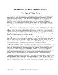
6 D-43883. CONVENTIONAL SUPPLY AND DEMAND3.1 IntroductionThis section deals with supply and demand as sometimes taught in high-schooleconomics classes. The following descriptions of supply and demand assume a perfectlycompetitive market, rational consumers, and free entry and exit into the market.Economists also make the simplification that all factors other than price which affect thequantity of goods sold and purchased are held constant. Economists argue that this is avalid assumption because changes in price occur much more quickly than changes inother factors that may affect supply or demand. Examples of these other factors includechanges in taste, changes in the state of the economy and long-term changes inproduction capacity (such as the construction of a new factory).3.2 DemandDemand is the rate at which consumers want to buy a product. Economic theoryholds that demand consists of two factors: taste and ability to buy. Taste, which is thedesire for a good, determines the willingness to buy the good at a specific price. Abilityto buy means that to buy a good at specific price, an individual must possess sufficientwealth or income.Both factors of demand depend on the market price. When the market price for aproduct is high, the demand will be low. When price is low, demand is high. At verylow prices, many consumers will be able to purchase a product. However, people usuallywant only so much of a good. Acquiring additional increments of a good or service insome time period will yield less and less satisfaction. 3 As a result, the demand for aproduct at low prices is limited by taste and is not infinite even when the price equalszero. As the price increases, the same amount of money will purchase fewer products.When the price for a product is very high, the demand will decrease because, whileconsumers may wish to purchase a product very much, they are limited by their ability tobuy.The curve in Figure 1 shows a generalized relationship between the price of agood and the quantity which consumers are willing to purchase in a given time period.This is known as a simple demand curve.3 This behavior toward aquiring additional increments of a good is called diminishing marginal utility.

D-4388 7Demand Limited byability to buyPriceDemand Limitedby tasteRate of PurchaseFigure 1: Demand Curve 4This curve shows the rate at which consumers wish to purchase a product at a givenprice.The simple demand curve seems to imply that price is the only factor whichaffects demand. Naturally, this is not the case. Recall the assumption made byeconomists that the other factors which influence changes in demand act over a muchlarger time frame. These factors are assumed to be constant over the time period inwhich price causes supply and demand to stabilize.4 The reader should note that the convention in economic theory is to plot the price on the vertical axis andthe rate of purchase on the horizontal axis.

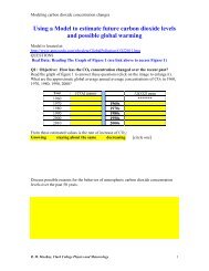
Price8 D-43883.3 SupplyWillingness and ability to supply goods determine the seller’s actions. At higherprices, more of the commodity will be available to the buyers. This is because thesuppliers will be able to maintain a profit despite the higher costs of production that mayresult from short-term expansion of their capacity 5 .In a real market, when the inventory is less than the desired inventory,manufacturers will raise both the supply of their product and its price. The short-termincrease in supply causes manufacturing costs to rise, leading to a further increase inprice. The price change in turn increases the desired rate of production. A similar effectoccurs if inventory is too high. Classical economic theory has approximated thiscomplicated process through the supply curve. The supply curve shown in Figure 2slopes upward because each additional unit is assumed to be more difficult or expensiveto make than the previous one, and therefore requires a higher price to justify itsproduction.SupplyFigure 2: Supply CurveAt high prices, there is more incentive to increase production of a good. This graphrepresents the short-term approximation of classical economic theory.5 Short-term expansion can be achieved by giving workers overtime hours, contracting to an outside source,or increasing the load on current equipment. These types of changes increase per-unit supply costs.

D-4388 93.4 Interaction Between Supply and DemandDemand is defined as the quantity (or amount) of a good or service people arewilling and able to buy at different prices, while supply is defined as how much of a goodor service is offered at each price. How do they interact to control the market?Buyers and sellers react in opposite ways to a change in price. When priceincreases, the willingness and ability of sellers to offer goods will increase, while thewillingness and ability of buyers to purchase goods will decrease. To illustrate moreclearly how the market works, we will look at the following example from the clothingindustry.Table 1 is called a schedule of demand and supply. For each price, it indicateshow much clothing is demanded by the consumers per week, and how much clothing issupplied per week. Notice that as price decreases, demand increases and supplydecreases. Eventually demand exceeds supply.

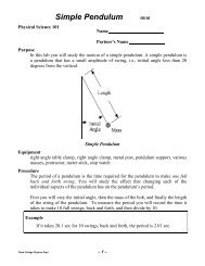
10 D-4388Demand and Supply SchedulesPrice Quantity QuantityDemandedSupplied(per week)(per week)---------------------------------------------------------------$50 10 100$45 14 97$40 18 94$35 22 89$30 28 84$25 35 77$20 45 68$15 57 57$10 73 40$5 100 0Table 1: Demand and Supply SchedulesFor each price, the schedule above indicates the quantity (in articles per week) of clothingdemanded and supplied.The market will reach equilibrium when the quantity demanded and the quantitysupplied are equal. At $15, supply and demand are equal at 57 articles of clothing perweek. To better understand the dynamics involved, suppose that one article of clothingwas selling for $30. Producers would be willing to supply 84 articles of clothing perweek, but consumers would only be buying 28 articles per week. As a result, theproducers would have excess inventory piling up very quickly. In order to get theirinventory back to the desired level, the suppliers would have to decrease production andreduce the price. Eventually, the quantity demanded and quantity supplied meet at 57articles per week at a price of $15.

D-4388 11$50DemandSupplyPrice per article of Clothing ($)$40$30$20$10$0Equilibrium PriceEquilibriumQuantityEquilibrium Point0 20 40 60 80 100Quantity of Clothing per weekFigure 3: Demand and Supply CurvesThese curves were plotted from the data for the clothing market included in Table 1.Figure 3 plots the demand and supply curves from the data in Table 1. Notice thatat $15 the supply and demand curves meet.

12 D-43884. A SYSTEM DYNAMICS APPROACH TOSUPPLY AND DEMAND4.1 IntroductionClassical economic theory presents a model of supply and demand that explainsthe equilibrium of a single product market. The dynamics involved in reaching thisequilibrium are assumed to be too complicated for the average high-school student.Economists hold the view that price determines both the supply and the demand.Equlibrium economics defines only the intersection of the supply and demand curves, nothow that intersection is reached.On the other hand, system dynamicists believe that the availability of a product,rather than its rate of production, affects the market price and demand. This means thatthe inventory (or backlog) of a product is a major determinant in setting price andregulating demand. This model is a hybrid of both views in that it introduces thedynamic effects of inventory into a model that generally replicates the economists’ staticexplanation of supply and demand.To explore the dynamics of supply and demand we will use the clothing market asan example. Because of a very aggressive marketing campaign, demand for clothes hasincreased. How will the suppliers and consumers react?To study the behavior of the market, we will look at its three major components:supply, demand, and price. There will be a series of exercises to help you understand themodel. We will first look at consumer demand.

D-4388 134.2 DemandDemandinventoryshipmentsdemanddemand price scheduledesired inventory~priceFigure 4: Demand SectorDemand in this model obeys one simple rule. It is the demand as dictated by thedemand price schedule. The demand price schedule is a demand curve that indicateswhat quantity consumers are willing to buy at a given price. The demand directly affectstwo things. First, it determines the outflow to the inventory stock of the suppliers. Thismodel assumes that the rate of shipments from the inventory is equal to the demand.Additionally, the demand sets the size of the supplier’s desired inventory.

14 D-4388Figure 5 shows the simple demand curve used in the demand price schedulegraphical function. This curve is somewhat different from the curve shown in Figure 1.Because STELLA and system dynamics standard practice require the input to a graphicalfunction to be on the horizontal axis, it was necessary to reverse the axes. In the curveshown in Figure 5, price is on the horizontal axis instead of the vertical. As discussedearlier, the curve shows that consumers are willing to buy more if the price is lower.Figure 5: Demand Price ScheduleThis curve is a simple demand curve from classical economics with the axes reversed.

D-4388 154.3 SupplyBelow is the supply sector of the model. To simplify the model, we combined theinventories of all the suppliers into one large inventory. The inflow supply represents thetotal production of goods to inventory. The outflow to this stock, shipments, is equal tothe demand.SupplyDemandsupplyinventoryshipmentsdemandinventory ratio~supply price scheduledesired inventorydemand price schedule~desired inventory coveragepriceFigure 6: Supply SectorIn Section 3 (Conventional Supply and Demand, page 8) there was no discussionof inventory. Basic classical economic theory does not specifically address the effects ofexcess or inadequate inventory. This model includes these effects. The inventory stockrepresents the total quantity of clothing in the warehouses of all suppliers.The shipments flow is equal to the weekly demand for clothing. Desiredinventory is the quantity of clothing the suppliers would like to have in inventory. Thesuppliers like to have enough inventory to cover several weeks of demand. Therefore,desired inventory is the product of desired inventory coverage and demand. Theinventory ratio is the ratio of inventory to desired inventory. The inventory ratio will beused to determine price later in the modeling process.

16 D-4388Before clothes can be stored in the warehouses, they need to be produced. Thesupply flow is determined by the supply price schedule. The supply price schedule is asupply curve which indicates how much the producers are willing to produce for eachprice they receive in the market. The source for this relation is the supply curve providedby classical economic theory 6 . As with the demand curve, the axes must be reversed sothat price can be an input to the graphical function. The curve used in the supply priceschedule is shown in Figure 7 below.Figure 7: Supply Price ScheduleThis curve was derived by taking the simple supply curve from classical economics andreversing the axes. This curve shows the rate of production for a given price.Below a certain price, the incentive to produce is zero because manufacturerscannot cover the costs of production. As the price rises above that cutoff, supply willincrease rapidly. At higher prices, the additional cost of increasing the supply begins tooutweigh the benefits of selling at a higher price. As the supply rate continues to6 The reader should note that this curve is being used in place of more complictated dynamic structure.There is no real-world causal relation between the price and the supply rate of a product. The informationcontained in the graph is an approximation for the behavior that would be produced by including structurewhich includes the effects of varying production capacity and employment.

D-4388 17increase, it takes larger and larger increases in the market price to justify further increasesin supply.

18 D-43884.4 Interaction between Supply and DemandSupplyDemandsupplyinventoryshipmentsdemandinventory ratio~supply price scheduledesired inventorydemand price schedule~desired inventory coveragePriceeffect on pricedesired price~price change delaypricechange in priceFigure 8: Price SectorPrice affects supply and demand as determined by the supply price schedule andthe demand price schedule. When price is high, demand is low and supply is high. Whenprice is low, demand is high and supply is low. We assumed that the only direct actionby a manufacturer to bring inventory to the desired level is to vary price.The action of the suppliers to regulate the price based on the inventory ratio isshown in Figure 9. Recall that the inventory ratio is defined as the ratio of inventory todesired inventory.

D-4388 19Figure 9: Effect on Price graphical functionWhen there is excess inventory, the price is lowered and when there is inadequateinventory, the price is raised.The graphical function shown in Figure 9 represents the action of suppliers toregulate their inventory. When inventory is below the desired inventory, then theinventory ratio is less than one. The graph in Figure 9 shows that an inventory ratio lessthan 1 gives a value for effect on price that is greater than one. This causes the price toincrease. The increase in price causes the supply to increase and the demand to decreasethrough their respective price schedules and brings the inventory closer the desired value.Multiplying the output of the effect on price converter and actual price returns desiredprice.Price was modeled as a stock because prices cannot change instantaneously.People do not have immediate and exact information on the supply (inventory) anddemand of the commodity in question. Additionally, when the information becomesavailable, it takes time to make a decision about changing the price.

20 D-43885. TESTING THE MODELPutting the model together, we get the following:Supply and DemandSupplyDemandsupplyinventoryshipmentsdemandInventory Ratio~supply price scheduledesired inventorydemand price schedule~desired inventory coveragePriceeffect on pricedesired price~price change delaypricechange in priceFigure 10: The complete Supply and Demand model

D-4388 21At this point, you may wish to build the STELLA model of supply and demand.The exercises that follow do not require you to run the model, but you may wish toperform some simulations of your own. The complete model equations are included inthe appendix, beginning on page 33.You will analyze three scenarios in this section. The first scenario will be a basecase run to observe the response of the model to a step increase in demand. Then youwill analyze how the behavior of the system varies from the base case when you changethe desired inventory coverage and the price change delay. Solutions start on page 28.5.1 Increase in DemandFor the base case run, assume the following conditions:• initial price = $15 per article of clothing• desired inventory coverage = 4 weeks• price change delay = 15 weeks#1: What should inventory be in order for the system to be in equilibrium? (Hint: lookat the supply price schedule and the demand price schedule) _______________________Discuss your reasoning below.________________________________________________________________________________________________________________________________________________________________________________________________________________________________________________________________________________________________________________________________________________________________________#2: Assume that the system is in equilibrium. Price and inventory remain the sameuntil the tenth week, at which time there is a permanent increase in demand of 10 units.(At each price, the consumer demand is 10 articles per week higher.) What are the newequilibrium values for price and inventory? ____________________________________

22 D-4388#3: Draw below what you think will happen to inventory in response to an increase indemand.1 : invent ory400.00200.0010.000.00 50.00 100.00 150.00 200.00WeeksExplain your reasoning:________________________________________________________________________________________________________________________________________________________________________________________________________________________________________________________________________________________________________________________________________________________________________

D-4388 235.2 Desired Inventory CoverageWe will now explore the response of the system to an increase in demand fordifferent values of the desired inventory coverage (the number of weeks of desiredinventory coverage). Presently desired inventory coverage is 4 weeks and the system isin equilibrium. The response of the system to a step increase in demand with desiredinventory coverage = 4 weeks is shown below.#4: If we change desired inventory coverage to 6 weeks, how would the system reactto the same increase in demand? On the graph below, draw the expected behavior.#5: Now, draw on the same graph what you expect the behavior of inventory will be ifdesired inventory coverage is equal to 2 weeks and there is an increase in demand.1 : invent ory400.00200.0011110.000.00 50.00 100.00 150.00 200.00WeeksExplain your reasoning:________________________________________________________________________________________________________________________________________________________________________________________________________________________________________________________________________________________________________________________________________________________________________

24 D-43885.3 Price Change DelayWe are now ready to discuss the effect of varying the price change delay. Thedelay obviously affects how quickly the price changes, and in the following exercises wewill see how well you can predict the behavior of price when that delay is modified.#6: Currently, the price change delay is 15 weeks. Assuming everything else remainsunchanged (system in equilibrium), would price or inventory change over time if thedelay is suddenly shortened? __________________Why or why not?________________________________________________________________________________________________________________________________________________________________________________________________________________________________________________________________________________________________________________________________________________________________________#7: Would you expect the system to reach equilibrium more quickly when the pricechange delay is equal to 30 weeks or 15 weeks? ____________Explain your reasoning:________________________________________________________________________________________________________________________________________________________________________________________________________________________________________________________________________________________________________________________________________________________________________

D-4388 25The graph below shows the response of the system to a step increase in demand when theprice change delay is 15 weeks.#8: If the price change delay is changed to 5 weeks, how would the system react to anincrease in demand? On the graph below, draw the expected behavior of price.#9: Now, draw on the same graph what you expect the behavior of price to be if pricechange delay is changed to 30 weeks and there is an increase in demand.1: price20.0017.5011115.0010.00 50.00 100.00 150.00 200.00WeeksExplain your reasoning:________________________________________________________________________________________________________________________________________________________________________________________________________________________________________________________________________________________________________________________________________________________________________

26 D-43885.4 Further ExplorationNaturally, no system dynamics model is ever complete. We believe that themodel presented is adequate for the purposes of this paper, but there are manypossibilities for enhancing it. One possibility is to include the effect of availableinventory on demand. The current model assumes that if a product is not currentlyavailable, the consumer will simply place an order and wait for the product to arrive,creating negative inventory, or backlog. You may also wish to include structure forincreasing the capacity of the supplier. This would allow for increased productionwithout raising the per-item cost. You could also experiment with the dynamics of a nondurablegood market (i.e., food). The possibilities are unlimited and it will help enhanceyour modeling skills.

D-4388 276. SOLUTIONS TO EXERCISES6.1 Increase in Demand#1: In equilibrium, all stocks must remain constant. The price will remain constantwhen the inventory ratio is one. Therefore, in equilibrium, the inventory is equal to thedesired inventory. By looking at the supply and demand curves contained in thegraphical functions of Demand Price Schedule and Supply Price Schedule we can see thatthe equilibrium price is $15 when demand and production both equal 57 articles ofclothing per week. Since the desired inventory coverage is 4 weeks, the equilibriuminventory is 228 articles of clothing.#2: An increase in demand of 10 articles of clothing per week means that the demandcurve in the demand price schedule is shifted up by 10. An easy way to figure out thenew equilibrium price is to plot the supply curve and the new demand curve on the samegraph and find the intersection. Doing this shows that the new equilibrium price will beabout $17 with production and demand slightly less than 62 articles per week. The newequilibrium inventory is then 62*4 or 248 articles of clothing.

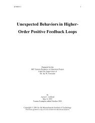
28 D-43881 : invent ory400.00200.0011110.000.00 50.00 100.00 150.00 200.00WeeksFigure 11: Step in DemandInventory decreases at first due to increased demand. It then overshoots and oscillates toa new equilibrium.#3: The increase in demand causes the desired inventory to immediately shoot up by40 articles of clothing (10 articles per week * 4 weeks of coverage). At the same time,inventory begins to drop because shipments are higher than supply. These cause theinventory ratio to drop, resulting in an increase in price. The price increase causes thedemand to fall and supply to increase allowing the inventory to catch up to the desiredinventory. However, the price continues to rise until the inventory has overshot itsequilibrium value. At this point the inventory ratio becomes positive, causing the price tobegin falling. Although the price is falling, it remains above its equilibrium valuecausing the inventory to continue increasing beyond its equilibrium. Eventually, theprice falls below the equilbrium price and causes the inventory to begin decreasing, butthe inventory again overshoots and the system oscillates to its new equilibrium withinventory equal to about 248. A graph of this behavior is shown in Figure 11.

D-4388 296.2 Desired Inventory Coverage#4 & #5: The desired inventory coverage affects the size of the desired inventory.The response of the system to an increase in demand was very different for the threevalues of desired inventory coverage. When the desired inventory coverage was 2weeks, the inventory seemed to exhibit sustained oscillation. As the coverage wasincreased to 4 and 6 weeks, the reaction to an increase in demand was smaller andstabilized more quickly. This behavior shows that there is a tradeoff when consideringthe size of inventory coverage. When the desired inventory coverage is high, inventoryremains fairly stable and is not greatly affected by changes in demand. Unfortunately,maintaining a large inventory can be costly. Lower values for desired inventory coverageare less costly to maintain, but react dramatically to changes in demand. Figure 12 showsthe model runs for desired inventory coverage equal to 2, 4 and 6 weeks. (Curves 1, 2and 3 respectively.)1 : invent ory 2 : invent ory 3 : invent ory400.003 3 33222200.0021 1 110.000.00 50.00 100.00 150.00 200.00WeeksFigure 12: Change in desired inventory coverageVariations in desired inventory coverage have a large effect on the behavior of thesystem. Higher coverage allows the inventory to maintain stable, but is costly tomaintain.

30 D-43886.3 Price Change Delay#6: The price change delay does not affect the equilibrium state of the model. Thisdelay only comes into effect when the price is changing. Any change in the price changedelay will not affect the model if it is already in equilibrium.#7: When the model is knocked out of equilibrium, the price change delay affectshow it approaches its new equilibrium. When the price change delay is short (5 weeks),the price changes rapidly and overshoots its equilibrium value. The price also convergeson its equilibrium quickly. As the price change delay increases (15 weeks and 30weeks), the changes are more gradual, the overshoot smaller and the equilibrium takeslonger to reach.

D-4388 31#8, #9: The graphs below show the reaction of price to an increase in demand when theprice change delay is 5, 15 and 30 weeks.1: price20.0017.501 1 15 Weeks1: price15.0020.0010.00 50.00 100.00 150.00 200.00Weeks17.501115 Weeks11: price15.0020.0010.00 50.00 100.00 150.00 200.00Weeks17.5030 Weeks11115.0010.00 50.00 100.00 150.00 200.00WeeksFigure 13: Variations in price change delay

32 D-43887. APPENDIX7.1 Model EquationsDemand Sectordemand = demand_price_schedule+step(10,10)DOCUMENT: This is the rate at which consumers wish to purchase clothing from thecompany. The step function is used to jar the system out of equilibrium.UNITS: shirts per weekdemand_price_schedule = GRAPH(price)(5.00, 100), (10.0, 73.0), (15.0, 57.0), (20.0, 45.0), (25.0, 35.0), (30.0, 28.0), (35.0, 22.0),(40.0, 18.0), (45.0, 14.0), (50.0, 10.0)DOCUMENT: This is based on the simple demand curve. At some particular price, theconsumers are willing and able to purchase clothing at a certain rate; the lower the price,the higher the demand.UNITS: shirts per weekPrice Sectorprice(t) = price(t - dt) + (change_in_price) * dtINIT price = 15DOCUMENT: Price is modeled as a stock in order to model the delays inherent inchanges in price.UNITS : dollars per shirtINFLOWS:change_in_price = ((desired_price)-price)/price_change_delayDOCUMENT: Change in price can be either positive or negative depending onthe effect_on_price. If the effect_on_price > 1, then price will increase. If theeffect_on_price < 1, then the price decreases. If effect_on_price = 1, priceremains same. Price changes slowly, so we divide the change byprice_change_delay.UNITS: price/week or ($/shirt)/weekdesired_price = effect_on_price*priceDOCUMENT: This is the equilibrium price as set by the inventory_ratio. The actualprice will reach this value after a delay specified by the price_change_delay.UNITS: dollars per shirtprice_change_delay = 15DOCUMENT: Prices do not change instantaneously.quickly price can change.UNITS : weeksThis value determines how

D-4388 33effect_on_price = GRAPH(inventory_ratio)(0.5, 2.00), (0.6, 1.80), (0.7, 1.55), (0.8, 1.35), (0.9, 1.15), (1, 1.00), (1.10, 0.875), (1.20,0.75), (1.30, 0.65), (1.40, 0.55), (1.50, 0.5)DOCUMENT: This graphical function regulates price change. When the inventory >desired_inventory then the inventory_ratio is >1 and price must be reduced. When theinventory ratio is

34 D-43887.2 Typical Model BehaviorThese graphs represent the behavior of the model set up with the values in theequations listed above. The model is initialized in equilibrium and there is a step increasein demand of 10 units/week after 10 weeks.1 : invent ory 2 : desired invent ory 3 : invent ory rat io400.003.00200.001.501212121 23 3330.000.000.00 50.00 100.00 150.00 200.00Weeks1 : shipment s 2 : supply70.0060.002121212150.000.00 50.00 100.00 150.00 200.00Weeks

D-4388 351 : price 2 : desired price30.00220.00112121210.000.00 50.00 100.00 150.00 200.00Weeks