Student Notes To Accompany MS4214: STATISTICAL INFERENCE
Student Notes To Accompany MS4214: STATISTICAL INFERENCE
Student Notes To Accompany MS4214: STATISTICAL INFERENCE

Create successful ePaper yourself
Turn your PDF publications into a flip-book with our unique Google optimized e-Paper software.
Outline Solutions<br />
1. The cdf is F (t) = P (T ≤ t) = � t<br />
0 λe−λυ dυ = λ � − 1<br />
λ e−λυ� t<br />
0 = 1 − e−λυ . Next<br />
P (a ≤ T ≤ b) = F (b) − F (a) = e −λa − e −λb . Assume all settlements are inde-<br />
pendent. Then P (50 in first week) = {F (1)} 50 = (1 − e −λ ) 50 , because T ≤ 1<br />
for these 50 settlements. Likewise, 1 < T ≤ 2, for the 35 in the second week,<br />
so we have P (35 in second week) = {F (2) − F (1)} 35 = (e −λ − e −2λ ) 35 . The re-<br />
maining 15 have T > 2, which has probability 1 − P (T ≤ 2) = e −2λ , and thus<br />
P (15 after week two) = (e −2λ ) 15 . The likelihood function is therefore the product<br />
L(λ) = (1 − e −λ ) 50 (e −λ − e −2λ ) 35 (e −2λ ) 15 . Taking logarithms (always based e),<br />
∴ d<br />
dλ<br />
ln L(λ) = 50 ln(1 − e −λ ) + 35 ln � e −λ (1 − e −λ ) � + 15 ln(e −2λ )<br />
= 85 ln(1 − e −λ ) − (35 + 30)λ = 85 ln(1 − e −λ ) − 65λ.<br />
85e−λ<br />
85<br />
ln L(λ) = − 65 =<br />
1 − e−λ e−λ − 65.<br />
− 1<br />
Equating to zero, 85 = 65(e −λ − 1) or e λ = 150/65, so that ˆ λ = ln(150/65) =<br />
0.836. This is indeed a maximum; e.g. d2<br />
dλ 2 ln L(λ) = −85/(e λ − 1) 2 < 0 ∀ λ. Next<br />
1 − e −0.836 = 0.5666; e −0.836 − e −1.672 = 0.43344 − 0.18787 = 0.2456. Hence out of<br />
100 invoices, 56.66, 24.56 and 18.78 would be expected to be paid, on this model,<br />
in weeks 1, 2 and later. The actual numbers were 50, 35 and 15. The prediction<br />
for the second week is a long way from what happened, balanced by smaller<br />
discrepancies in the other two periods. This does not seem very satisfactory.<br />
2. nA + nB = n ⇒ nB = n − nA. Suppose we observe the sequence A, B, A, B, A,<br />
then L1(nA) = nA<br />
n<br />
× n−nA<br />
n−1<br />
× nA−1<br />
n−2<br />
× n−nA−1<br />
n−3<br />
sequence A, A, B, B, A, then L2(nA) = nA<br />
n<br />
nA−2<br />
× . Next, suppose we observe the<br />
n−4<br />
× nA−1<br />
n−1<br />
× n−nA<br />
n−2<br />
× n−nA−1<br />
n−3<br />
nA−2<br />
× n−4<br />
. If it<br />
is known that 3As and 2Bs are drawn but the exact sequence is unknown then<br />
L3(nA) = P (Y = y|nA) = � �� � � � nA n−nA n<br />
/ , where y = 3. This third likelihood<br />
y 5−y 5<br />
function expands to give L3(nA) = 10 × nA(nA−1)(nA−2)(n−nA)(n−nA−1)<br />
. Clearly<br />
n(n−1)(n−2)(n−3)(n−4)<br />
L1(nA) = L2(nA) = L3(nA) ÷ 10. The first two likelihood functions are identical.<br />
The third likelihood function is a constant times the other two, and as only the<br />
ratio of likelihood functions are meaningful, L3(nA) carries the same information<br />
about our preferences for the parameter nA as the other functions.<br />
3. L(θ) = 4 −n (2 + θ) a (1 − θ) b+c (θ) d so, ℓ(θ) = −n ln(4)+a ln(2+θ)+(b+c) ln(1−<br />
θ) + d ln(θ). Differentiating we get S(θ) = a b+c d − + and setting S(θ) = 0<br />
2+θ 1−θ θ<br />
leads to the quadratic equation nθ2 − {a − 2b − 2c − d}θ − 2d = 0, of which<br />
the positive root, ˆ θ, satisfies the condition of maximum likelihood. If S(θ) is<br />
differentiated again with respect to θ, and expected values substituted for a, b, c,<br />
and d, we obtain Var( ˆ θ) ≈ {E[I(θ)]} −1 = {I(θ)} −1 = 2θ(1−θ)(2+θ)<br />
(1+2θ)n<br />
45<br />
.