Student Notes To Accompany MS4214: STATISTICAL INFERENCE

Student Notes To Accompany
MS4214: STATISTICAL INFERENCE
Dr. Kevin Hayes
September 1, 2007

Contents
1 Introduction 3
1.1 Motivating Examples . . . . . . . . . . . . . . . . . . . . . . . . . . . . 3
1.2 General Course Overview . . . . . . . . . . . . . . . . . . . . . . . . . . 6
2 The Theory of Estimation 8
2.1 The Frequentist Philosophy . . . . . . . . . . . . . . . . . . . . . . . . 8
2.2 The Frequentist Approach to Estimation . . . . . . . . . . . . . . . . . 10
2.3 Minimum-Variance Unbiased Estimation . . . . . . . . . . . . . . . . . 14
2.4 Maximum Likelihood Estimation . . . . . . . . . . . . . . . . . . . . . 18
2.5 Multi-parameter Estimation . . . . . . . . . . . . . . . . . . . . . . . . 28
2.6 Newton-Raphsom Optimization . . . . . . . . . . . . . . . . . . . . . . 31
2.7 The Invariance Principle . . . . . . . . . . . . . . . . . . . . . . . . . . 38
2.8 Optimality Properties of the MLE . . . . . . . . . . . . . . . . . . . . . 39
2.9 Data Reduction . . . . . . . . . . . . . . . . . . . . . . . . . . . . . . . 39
2.10 Worked Problems . . . . . . . . . . . . . . . . . . . . . . . . . . . . . . 42
3 The Theory of Confidence Intervals 50
3.1 Exact Confidence Intervals . . . . . . . . . . . . . . . . . . . . . . . . . 50
3.2 Pivotal Quantities for Use with Normal Data . . . . . . . . . . . . . . . 53
3.3 Approximate Confidence Intervals . . . . . . . . . . . . . . . . . . . . 58
3.4 Worked Problems . . . . . . . . . . . . . . . . . . . . . . . . . . . . . . 60
4 The Theory of Hypothesis Testing 64
4.1 Introduction . . . . . . . . . . . . . . . . . . . . . . . . . . . . . . . . . 64
4.2 The General Testing Problem . . . . . . . . . . . . . . . . . . . . . . . 65
4.3 Hypothesis Testing for Normal Data . . . . . . . . . . . . . . . . . . . 66
4.4 Generally Applicable Test Procedures . . . . . . . . . . . . . . . . . . . 71
4.5 The Neyman-Pearson Lemma . . . . . . . . . . . . . . . . . . . . . . . 74
4.6 Goodness of Fit Tests . . . . . . . . . . . . . . . . . . . . . . . . . . . . 76
4.7 The χ 2 Test for Contingency Tables . . . . . . . . . . . . . . . . . . . . 79
1

4.8 Worked Problems . . . . . . . . . . . . . . . . . . . . . . . . . . . . . . 81
A Review of Probability 88
A.1 Expectation and Variance . . . . . . . . . . . . . . . . . . . . . . . . . 88
A.2 Discrete Random Variables . . . . . . . . . . . . . . . . . . . . . . . . . 89
A.2.1 Bernoulli Distribution . . . . . . . . . . . . . . . . . . . . . . . 89
A.2.2 Binomial Distribution . . . . . . . . . . . . . . . . . . . . . . . 89
A.2.3 Geometric Distribution . . . . . . . . . . . . . . . . . . . . . . . 90
A.2.4 Negative Binomial Distribution . . . . . . . . . . . . . . . . . . 91
A.2.5 Hypergeometric Distribution . . . . . . . . . . . . . . . . . . . . 91
A.2.6 Poisson Distribution . . . . . . . . . . . . . . . . . . . . . . . . 92
A.2.7 Discrete Uniform Distribution . . . . . . . . . . . . . . . . . . . 93
A.2.8 The Multinomial Distribution . . . . . . . . . . . . . . . . . . . 93
A.3 Continuous Random Variables . . . . . . . . . . . . . . . . . . . . . . . 94
A.3.1 Uniform Distribution . . . . . . . . . . . . . . . . . . . . . . . . 94
A.3.2 Exponential Distribution . . . . . . . . . . . . . . . . . . . . . . 94
A.3.3 Gamma Distribution . . . . . . . . . . . . . . . . . . . . . . . . 95
A.3.4 Gaussian Distribution . . . . . . . . . . . . . . . . . . . . . . . 96
A.3.5 Weibull Distribution . . . . . . . . . . . . . . . . . . . . . . . . 98
A.3.6 Beta Distribution . . . . . . . . . . . . . . . . . . . . . . . . . . 98
A.3.7 Chi-square Distribution . . . . . . . . . . . . . . . . . . . . . . 99
A.3.8 Distribution of a Function of a Random Variable . . . . . . . . 99
A.4 Random Vectors . . . . . . . . . . . . . . . . . . . . . . . . . . . . . . 101
A.4.1 Sums of Independent Random Variables . . . . . . . . . . . . . 101
A.4.2 Covariance and Correlation . . . . . . . . . . . . . . . . . . . . 104
A.4.3 The Bivariate Change of Variables Formula . . . . . . . . . . . 105
A.4.4 The Bivariate Normal Distribution . . . . . . . . . . . . . . . . 106
A.4.5 Bivariate Normal Conditional Distributions . . . . . . . . . . . 107
A.4.6 The Multivariate Normal Distribution . . . . . . . . . . . . . . 107
A.5 Generating Functions . . . . . . . . . . . . . . . . . . . . . . . . . . . . 108
A.6 Table of Common Distributions . . . . . . . . . . . . . . . . . . . . . . 111
2

Chapter 1
Introduction
1.1 Motivating Examples
Example 1.1 (Radioactive decay). Let X denote the number of particles that will be
emitted from a radioactive source in the next one minute period. We know that X
will turn out to be equal to one of the non-negative integers but, apart from that, we
know nothing about which of the possible values are more or less likely to occur. The
quantity X is said to be a random variable.
Suppose we are told that the random variable X has a Poisson distribution with
parameter θ = 2. Then, if x is some non-negative integer, we know that the probability
that the random variable X takes the value x is given by the formula
P (X = x) = θx exp (−θ)
x!
where θ = 2. So, for instance, the probability that X takes the value x = 4 is
P (X = 4) = 24 exp (−2)
4!
= 0.0902 .
We have here a probability model for the random variable X. Note that we are using
upper case letters for random variables and lower case letters for the values taken by
random variables. We shall persist with this convention throughout the course.
Suppose we are told that the random variable X has a Poisson distribution with
parameter θ where θ is some unspecified positive number. Then, if x is some non-
negative integer, we know that the probability that the random variable X takes the
value x is given by the formula
P (X = x|θ) = θx exp (−θ)
, (1.1)
x!
for θ ∈ R + . However, we cannot calculate probabilities such as the probability that X
takes the value x = 4 without knowing the value of θ.
3

Suppose that, in order to learn something about the value of θ, we decide to measure
the value of X for each of the next 5 one minute time periods. Let us use the notation X1
to denote the number of particles emitted in the first period, X2 to denote the number
emitted in the second period and so forth. We shall end up with data consisting of a
random vector X = (X1, X2, . . . , X5). Consider x = (x1, x2, x3, x4, x5) = (2, 1, 0, 3, 4).
Then x is a possible value for the random vector X. We know that the probability that
X1 takes the value x1 = 2 is given by the formula
P (X = 2|θ) = θ2 exp (−θ)
2!
and similarly that the probability that X2 takes the value x2 = 1 is given by
θ exp (−θ)
P (X = 1|θ) =
1!
and so on. However, what about the probability that X takes the value x? In order for
this probability to be specified we need to know something about the joint distribution
of the random variables X1, X2, . . . , X5. A simple assumption to make is that the
random variables X1, X2, . . . , X5 are mutually independent. (Note that this assumption
may not be correct since X2 may tend to be more similar to X1 that it would be to
X5.) However, with this assumption we can say that the probability that X takes the
value x is given by
P (X = x|θ) =
5�
i=1
θxi exp (−θ)
,
xi!
= θ2 exp (−θ)
2!
× θ1 exp (−θ)
1!
× θ3 exp (−θ)
3!
× θ0 exp (−θ)
0!
× θ4 exp (−θ)
,
4!
= θ10 exp (−5θ)
.
288
In general, if X = (x1, x2, x3, x4, x5) is any vector of 5 non-negative integers, then the
probability that X takes the value x is given by
P (X = x|θ) =
5� θxi exp (−θ)
,
xi!
i=1
= θ� 5
i=1 xi exp (−5θ)
5�
xi!
We have here a probability model for the random vector X.
Our plan is to use the value x of X that we actually observe to learn something
about the value of θ. The ways and means to accomplish this task make up the subject
matter of this course. �
4
i=1
.

Example 1.2 (Tuberculosis). Suppose we are going to examine n people and record
a value 1 for people who have been exposed to the tuberculosis virus and a value 0
for people who have not been so exposed. The data will consist of a random vector
X = (X1, X2, . . . , Xn) where Xi = 1 if the ith person has been exposed to the TB virus
and Xi = 0 otherwise.
A Bernoulli random variable X has probability mass function
P (X = x|θ) = θ x (1 − θ) 1−x , (1.2)
for x = 0, 1 and θ ∈ (0, 1). A possible model would be to assume that X1, X2, . . . , Xn
behave like n independent Bernoulli random variables each of which has the same
(unknown) probability θ of taking the value 1.
Let x = (x1, x2, . . . , xn) be a particular vector of zeros and ones. Then the model
implies that the probability that the random vector X takes the value x is given by
P (X = x|θ) =
n�
θ xi 1−xi (1 − θ)
i=1
= θ �n i=1 xi n−
(1 − θ) �n i=1 xi .
Once again our plan is to use the value x of X that we actually observe to learn
something about the value of θ. �
Example 1.3 (Viagra). A chemical compound Y is used in the manufacture of Viagra.
Suppose that we are going to measure the micrograms of Y in a sample of n pills. The
data will consist of a random vector X = (X1, X2, . . . , Xn) where Xi is the chemical
content of Y for the ith pill.
A possible model would be to assume that X1, X2, . . . , Xn behave like n independent
random variables each having a N (µ, σ 2 ) density with unknown mean parameter µ ∈ R,
(really, here µ ∈ R + ) and known variance parameter σ 2 < ∞. Each Xi has density
fXi (xi|µ) =
1
√ 2πσ 2 exp
�
− (xi − µ) 2
2σ 2
Let x = (x1, x2, . . . , xn) be a particular vector of real numbers. Then the model implies
the joint density
fX(x|µ) =
=
n�
i=1
�
.
1
√
2πσ2 exp
�
− (xi − µ) 2 �
1
( √ 2πσ2 exp
) n
�
−
2σ 2
� n
i=1 (xi − µ) 2
2σ 2
Once again our plan is to use the value x of X that we actually observe to learn
something about the value of µ. �
5
�

Example 1.4 (Blood pressure). We wish to test a new device for measuring blood pres-
sure. We are going to try it out on n people and record the difference between the value
returned by the device and the true value as recorded by standard techniques. The
data will consist of a random vector X = (X1, X2, . . . , Xn) where Xi is the difference
for the ith person. A possible model would be to assume that X1, X2, . . . , Xn behave
like n independent random variables each having a N (0, σ 2 ) density where σ 2 is some
unknown positive real number. Let x = (x1, x2, . . . , xn) be a particular vector of real
numbers. Then the model implies that the probability that the random vector X takes
the value x is given by
fX(x|σ 2 ) =
=
n�
i=1
1
√
2πσ2 exp
�
− x2 i
1
( √ 2πσ2 exp
) n
�
−
2σ 2
�
� n
i=1 x2 i
2σ 2
Once again our plan is to use the value x of X that we actually observe to learn
something about the value of σ 2 . Knowledge of σ is useful since it allows us to make
statements such as that 95% of errors will be less than 1.96 × σ in magnitude. �
1.2 General Course Overview
Definition 1.1 (Inference). Inference studies the way in which data we observe
should influence our beliefs about and practices in the real world. �
Definition 1.2 (Statistical inference). Statistical inference considers how inference
should proceed when the data is subject to random fluctuation. �
The concept of probability is used to describe the random mechanism which gave
rise to the data. This involves the use of probability models.
The incentive for contemplating a probability model is that through it we may
achieve an economy of thought in the description of events enabling us to enunciate
laws and relations of more than immediate validity and relevance. A probability model
is usually completely specified apart from the values of a few unknown quantities called
parameters. We then try to discover to what extent the data can inform us about the
values of the parameters.
Statistical inference assumes that the data is given and that the probability model
is a correct description of the random mechanism which generated the data.
6
�
.

Three main topics will be covered :
Estimation Unbiasedness, mean square error, consistency, relative efficiency, suffi-
ciency, minimum variance. Fisher information for a function of a parameter,
Cramér-Rao lower bound, efficiency. Fitting standard distributions to discrete
and continuous data. Method of moments. Maximum likelihood estimation:
finding estimators analytically and numerically, invariance, censored data.
Hypothesis testing Simple and composite hypotheses, types of error, power, op-
erating characteristic curves, p-value. Neuman-Pearson method. Generalised
likelhood ratio test. Use of asympotic results to construct tests. Central limit
theorem, asymptotic distributions of maximum likelihood estimator and gener-
alised ratio test statistic.
Confidence intervals and sets Random intervals and sets. Use of pivotal qnatities.
Relationship between tests and confidence intervals. Use of asymptotic results.
7

Chapter 2
The Theory of Estimation
2.1 The Frequentist Philosophy
The dominant philosophy of inference is based on the frequentist theory of probability.
According to the frequentist theory probability statements can only be made regarding
events associated with a random experiment. A random experiment is an experiment
which has a well defined set of possible outcomes S. In addition, we must be able to en-
visage an infinite sequence of independent repetitions of the experiment with the actual
outcome of each repetition being some unpredictable element of S. A random variable
is a numerical quantity associated with each possible outcome in S. A random vector
is a collection of numerical quantities associated with each possible outcome in S. In
performing the experiment we determine which element of S has occurred and thereby
the observed values of all random variables or random vectors of interest. Since the
outcome of the experiment is unpredictable so too is the value of any random variable
or random vector. Since we can envisage an infinite sequence of independent repetitions
of the experiment, we can envisage an infinite sequence of independent determinations
of the value of a random variable (or vector). The purpose of a statistical model is to
describe the unpredictability of such a sequence of determinations.
Consider the random experiment which consists of picking someone at random from
the 2007 electoral register for Limerick. The outcome of such an experiment will be
a human being and the set S consists of all human beings whose names are on the
register. We can clearly envisage an infinite sequence of independent repetitions of
such an experiment. Consider the random variable X where X = 0 if the outcome
of the experiment is a male and X = 1 if the outcome of the experiment is a female.
When we say that P (X = 1) = 0.54 we are taken to mean that in an infinite sequence
of independent repetitions of the experiment exactly 54% of the outcomes will produce
a value of X = 1.
8

Now consider the random experiment which consists of picking 3 people at random
from the 1997 electoral register for Limerick. The outcome of such an experiment will
be a collection of 3 human beings and the set S consists of all subsets of 3 human
beings which may be formed from the set of all human beings whose names are on the
register. We can clearly envisage an infinite sequence of independent repetitions of such
an experiment. Consider the random vector X = (X1, X2, X3) where for i = 1, 2, 3,
Xi = 0 if the ith person chosen is a male and Xi = 1 if the ith person chosen is a
female. When we say that X1, X2, X3 are independent and identically distributed or IID
with P (Xi = 1) = θ we are taken to mean that in an infinite sequence of independent
repetitions of the experiment the proportion of outcomes which produce, for instance,
a value of X = (1, 1, 0) is given by θ 2 (1 − θ).
Suppose that the value of θ is unknown and we propose to estimate it by the
estimator ˆ θ whose value is given by the proportion of females in the sample of size 3.
Since ˆ θ depends on the value of X we sometimes write ˆ θ(X) to emphasise this fact.
We can work out the probability distribution of ˆ θ as follows :
X P (X = x) ˆ θ(x)
(0, 0, 0) (1 − θ) 3 0
(0, 0, 1) θ(1 − θ) 2 1/3
(0, 1, 0) θ(1 − θ) 2 1/3
(1, 0, 0) θ(1 − θ) 2 1/3
(0, 1, 1) θ 2 (1 − θ) 2/3
(1, 0, 1) θ 2 (1 − θ) 2/3
(1, 1, 0) θ 2 (1 − θ) 2/3
(1, 1, 1) θ 3 1
Thus P ( ˆ θ = 0) = (1 − θ) 3 , P ( ˆ θ = 1/3) = 3θ(1 − θ) 2 , P ( ˆ θ = 2/3) = 3θ 2 (1 − θ) and
P ( ˆ θ = 1) = θ 3 . We now ask whether ˆ θ is a good estimator of θ? Clearly if θ = 0 we
have that P ( ˆ θ = θ) = P ( ˆ θ = 0) = 1 which is good. Likewise if θ = 1 we also have that
P ( ˆ θ = θ) = P ( ˆ θ = 1) = 1. If θ = 1/3 then P ( ˆ θ = θ) = P ( ˆ θ = 1/3) = 3(1/3)(1−1/3) 2 =
4/9. Likewise if θ = 2/3 we have that P ( ˆ θ = θ) = P ( ˆ θ = 2/3) = 3(2/3) 2 (1−2/3) = 4/9.
However if the value of θ lies outside the set {0, 1/3, 2/3, 1} we have that P ( ˆ θ = θ) = 0.
Since ˆ θ is a random variable we might try to calculate its expected value E( ˆ θ) i.e.
the average value we would get if we carried out an infinite number of independent
repetitions of the experiment. We have that
E( ˆ θ) = 0P ( ˆ θ = 0) + (1/3)P ( ˆ θ = 1/3) + (2/3)P ( ˆ θ = 2/3) + 1P ( ˆ θ = 1) ,
= 0(1 − θ) 3 + (1/3)3θ(1 − θ) 2 + (2/3)3θ 2 (1 − θ) + 1θ 3 ,
= θ.
9

Thus if we carried out an infinite number of independent repetitions of the experiment
and calculate the value of ˆ θ for each repetition the average of the ˆ θ values would be
exactly θ,the true value of the parameter! This is true no matter what the actual value
of θ is. Such an estimator is said to be unbiased.
Consider the quantity L = ( ˆ θ − θ) 2 which might be regarded as a measure of
the error or loss involved in using ˆ θ to estimate θ. The possible values for L are
(0 − θ) 2 , (1/3 − θ) 2 , (2/3 − θ) 2 and (1 − θ) 2 . We can calculate the expected value of
L as follows:
E(L) = (0 − θ) 2 P ( ˆ θ = 0) + (1/3 − θ) 2 P ( ˆ θ = 1/3)
+(2/3 − θ) 2 P ( ˆ θ = 2/3) + (1 − θ) 2 P ( ˆ θ = 1)
= θ 2 (1 − θ) 3 + (1/3 − θ) 2 3θ(1 − θ) 2 + (2/3 − θ) 2 3θ 2 (1 − θ) + (1 − θ) 2 θ 3 ,
= θ(1 − θ)/3 .
The quantity E(L) is called the mean squared error ( MSE ) of the estimator ˆ θ. Since
the quantity θ(1 − θ) attains its maximum value of 1/4 for θ = 1/2, the largest value
E(L) can attain is 1/12 which occurs if the true value of the parameter θ happens to be
equal to 1/2; for all other values of θ the quantity E(L) is less than 1/12. If somebody
could invent a different estimator ˜ θ of θ whose MSE was less than that of ˆ θ for all
values of θ then we would prefer ˜ θ to ˆ θ.
This trivial example gives some idea of the kinds of calculations that we will be
performing. The basic frequentist principle is that statistical procedures should be
judged in terms of their average performance in an infinite series of independent repe-
titions of the experiment which produced the data. An important point to note is that
the parameter values are treated as fixed (although unknown) throughout this infinite
series of repetitions. We should be happy to use a procedure which performs well on
the average and should not be concerned with how it performs on any one particular
occasion.
2.2 The Frequentist Approach to Estimation
Suppose that we are going to observe a value of a random vector X. Let X denote the
set of possible values X can take and, for x ∈ X , let f(x|θ) denote the probability that
X takes the value x where the parameter θ is some unknown element of the set Θ.
The problem we face is that of estimating θ. An estimator ˆ θ is a procedure which
for each possible value x ∈ X specifies which element of Θ we should quote as an
estimate of θ. When we observe X = x we quote ˆ θ(x) as our estimate of θ. Thus ˆ θ is a
function of the random vector X. Sometimes we write ˆ θ(X) to emphasise this point.
10

Given any estimator ˆ θ we can calculate its expected value for each possible value of
θ ∈ Θ. An estimator is said to be unbiased if this expected value is identically equal to
θ. If an estimator is unbiased then we can conclude that if we repeat the experiment
an infinite number of times with θ fixed and calculate the value of the estimator each
time then the average of the estimator values will be exactly equal to θ. From the
frequentist viewpoint this is a desireable property and so, where possible, frequentists
use unbiased estimators.
Definition 2.1 (The Frequentist philosophy). To evaluate the usefulness of an
estimator ˆ θ = ˆ θ(x) of θ, examine the properties of the random variable ˆ θ = ˆ θ(X). �
Definition 2.2 (Unbiased estimators). An estimator ˆ θ = ˆ θ(X) is said to be unbi-
ased for a parameter θ if it equals θ in expectation:
E[ ˆ θ(X)] = E( ˆ θ) = θ.
Intuitively, an unbiased estimator is ‘right on target’. �
Definition 2.3 (Bias of an estimator). The bias of an estimator ˆ θ = ˆ θ(X) of θ is
defined as bias( ˆ θ) = E[ ˆ θ(X) − θ]. �
Definition 2.4 (Bias corrected estimators). If bias( ˆ θ) is of the form cθ, then
(obviously) ˜ θ = ˆ θ/(1 + c) is unbiased for θ. Likewise, if bias( ˆ θ) = θ + c, then ˜ θ = ˆ θ − c
is unbiased for θ. In such situations we say that ˜ θ is a biased corrected version of ˆ θ. �
Definition 2.5 (Unbiased functions). More generally ˆg(X) is said to be unbiased
for a function g(θ) if E[ˆg(X)] = g(θ). �
Note that even if ˆ θ is an unbiased estimator of θ, g( ˆ θ) will generally not be an
unbiased estimator of g(θ) unless g is linear or affine. This limits the importance of the
notion of unbiasedness. It might be at least as important that an estimator is accurate
in the sense that its distribution is highly concentrated around θ.
Is unbiasedness a good thing? Unbiasedness is important when combining esti-
mates, as averages of unbiased estimators are unbiased (see the review exercises at the
end of this chapter). For example, when combining standard deviations s1, s2, . . . , sk
with degrees of freedom df1, . . . , dfk we always average their squares
�
df1s
¯s =
2 1 + · · · + dfks2 k
df1 + · · · + dfk
as s 2 i are unbiased estimators of the variance σ 2 , whereas si are not unbiased estimators
of σ (see the review exercises). Be careful when averaging biased estimators! It may
well be appropriate to make a bias-correction before averaging.
11

Problem 2.1. Let X have a binomial distribution with parameters n and θ. Show
that the sample proportion ˆ θ = X/n is an unbiased estimate of θ.
Solution. X ∼ Bin(n, θ) ⇒ E(X) = nθ. Then E( ˆ θ) = E(X/n) = E(X)/n = nθ/n = θ.
As E( ˆ θ) = θ, the estimator ˆ θ is unbiased.
Problem 2.2. Let X1, . . . , Xn be independent and identically distributed with density
�
e
f(x|θ) =
−(x−θ) , for x > θ;
0, otherwise.
Show that ˆ θ = ¯ X = (X1 + · · · + Xn)/n is a biased estimator of θ. Propose an unbiased
estimator ˜ θ of the form ˜ θ = ˆ θ + c.
Solution. E(X) = � ∞
θ xe−(x−θ) dx = � −xe −(x−θ) + � e −(x−θ) dx � ∞
θ = −(x+1)e−(x−θ) | ∞ θ =
θ+1. Next, E( ˆ θ) = E( ¯ X) = 1
n E(X1 +X2 +· · ·+Xn) = θ+1 �= θ ⇒ ˆ θ is biased. Propose
˜θ = ¯ X − 1. Then E( ˜ θ) = E( ¯ X) − 1 = θ + 1 − 1 = θ and ˜ θ is unbiased.
Definition 2.6 (Mean squared error). The mean squared error of the estimator ˆ θ
is defined as MSE( ˆ θ) = E( ˆ θ − θ) 2 . Given the same set of data, ˆ θ1 is “better” than ˆ θ2 if
MSE( ˆ θ1) ≤ MSE( ˆ θ2) (uniformly better if true ∀ θ). �
Lemma 2.3 (The MSE variance-bias tradeoff). The MSE decomposes as
MSE( ˆ θ) = Var( ˆ θ) + Bias( ˆ θ) 2 .
Proof. The problem of finding minimum MSE estimators cannot be solved uniquely:
MSE( ˆ θ) = E( ˆ θ − θ) 2
= E{ [ ˆ θ − E( ˆ θ) ] + [ E( ˆ θ) − θ ]} 2
= E[ ˆ θ − E( ˆ θ)] 2 + E[E( ˆ θ) − θ] 2
�
+2 E [ ˆ θ − E( ˆ θ)][E( ˆ �
θ) − θ]
� ��
=0
�
= E[ ˆ θ − E( ˆ θ)] 2 + E[E( ˆ θ) − θ] 2
= Var( ˆ θ) + [E( ˆ θ) − θ] 2
� �� �
Bias( ˆ θ) 2
NOTE : This lemma implies that the mean squared error of an unbiased estimator
is equal to the variance of the estimator.
12

Problem 2.4. Consider X1, . . . , Xn where Xi ∼ N(θ, σ 2 ) and σ is known. Three
estimators of θ are ˆ θ1 = ¯ X = 1
n
� n
i=1 Xi, ˆ θ2 = X1, and ˆ θ3 = (X1 + ¯ X)/2. Pick one.
Solution. E( ˆ θ1) = 1
n [E(X1)+· · ·+E(Xn)] = 1
1
[θ+· · ·+θ] = [nθ] = θ, (unbiased). Next
n n
E( ˆ θ2) = E(X1) = θ, (unbiased). Finally E( ˆ θ3) = 1
2E � n+1
n X1 + 1
n [X2 + · · · + Xn] � =
�
1 n+1
2 n E(X1) + 1
n [E(X2) + · · · + E(Xn)] � = 1 n+1 n−1
{ θ + θ} = θ, (unbiased). All three
2 n n
estimators are unbiased. Although desirable from a frequentist standpoint, unbiased-
ness is not a property that helps us choose between estimators. To do this we must
examine some measure of loss like the mean squared error. For class of estimators
that are unbiased, the mean squared error will be equal to the estimation variance.
Calculate Var( ˆ θ1) = 1
n 2 [Var(X1) + · · · + Var(Xn)] = 1
n 2 [σ 2 + · · · + σ 2 ] = 1
n 2 [nσ 2 ] = 1
n σ2 .
Trivially Var( ˆ θ2) = Var(X1) = σ 2 . Finally Var( ˆ θ3) = (σ 2 /n + σ 2 )/4 + 2Cov( ¯ X, X1).
So ¯ X appears “best” in the sense that Var( ˆ θ) is smallest among these three unbiased
estimators.
Problem 2.5. Consider X1, . . . , Xn to be independent random variables with means
E(Xi) = µ + βi and variances Var(Xi) = σ 2 i . Such a situation could arise when Xi are
estimators of µ obtained from independent sources and βi is the bias of the estimator
Xi. Consider pooling the estimators of µ into a common estimator using the linear
combination ˆµ = w1X1 + w2X2 + · · · + wnXn.
(i) If the estimators are unbiased, show that ˆµ is unbiased if and only if � wi = 1.
(ii) In the case when the estimators are unbiased, show that ˆµ has minimum variance
when the weights are inversely proportional to the variances σ 2 i .
(iii) Show that the variance of ˆµ for optimal weights wi is Var(ˆµ) = 1/ �
i σ−2
i .
(iv) Consider the case when estimators may be biased. Find the mean square error
of the optimal linear combination obtained above, and compare its behaviour as
n → ∞ in the biased and unbiased case, when σ 2 i = σ 2 , i = 1, . . . , n.
Solution. E(ˆµ) = E(w1X1 + · · · + wnXn) = �
i wiE(Xi) = �
i wiµ = µ �
i wi so ˆµ is
unbiased if and only if �
i wi = 1. The variance of our estimator is Var(ˆµ) = �
i w2 i σ 2 i ,
which should be minimized subject to the constraint �
i wi = 1. Differentiating the
Lagrangian L = �
i w2 i σ 2 i − λ ( �
i wi − 1) with respect to wi and setting equal to zero
yields 2wiσ 2 i = λ ⇒ wi ∝ σ −2
i so that wi = σ −2
i /(�
j σ−2 j
). Then, for optimal weights we
get Var(ˆµ) = �
i w2 i σ2 i = ( �
i σ−4 i σ2 i )/( �
i σ−2 i )2 = 1/( �
i σ−2 i ). When σ2 i = σ2 we have
that Var(ˆµ) = σ2 /n which tends to zero for n → ∞ whereas bias(ˆµ) = � βi/n = ¯ β is
equal to the average bias and MSE(ˆµ) = σ 2 + ¯ β 2 . Therefore the bias tends to dominate
the variance as n gets larger, which is very unfortunate.
13

Problem 2.6. Let X1, . . . , Xn be an independent sample of size n from the uniform
distribution on the interval (0, θ), with density for a single observation being f(x|θ) =
θ −1 for 0 < x < θ and 0 otherwise, and consider θ > 0 unknown.
(i) Find the expected value and variance of the estimator ˆ θ = 2 ¯ X.
(ii) Find the expected value of the estimator ˜ θ = X(n), i.e. the largest observation.
(iii) Find an unbiased estimator of the form ˇ θ = cX(n) and calculate its variance.
(iv) Compare the mean square error of ˆ θ and ˇ θ.
Solution. ˆ θ has E( ˆ θ) = E(2 ¯ X) = 2
n [E(X1) + · · · + E(Xn)] = 2 [(θ/2) + · · · + (θ/2)] =
n
2
n [n(θ/2)] = θ (unbiased), and Var(ˆ θ) = Var(2 ¯ X) = 4
n2 [Var(X1) + · · · + Var(Xn)] =
4
n2 [(θ2 /12) + · · · + (θ2 /12)] = 4
n2 n
12θ2 = 1
3nθ2 . Let U = X(n), we then have P (U ≤ u) =
�n i P (Xi ≤ u) = (u/θ) n for 0 < u < θ so differentiation yields that U has density
f(u|θ) = nun−1θ−n for 0 < u < θ. Direct integration now yields E( ˜ θ) = E(U) = n
n+1θ (a biased estimator). The estimator ˇ θ = n+1 U is unbiased. Direct integration gives
E(U 2 ) = n
n+2θ2 so Var( ˜ n
θ) = Var(U) = (n+2)(n+1) 2 θ2 and Var( ˇ θ) = 1
n(n+2) θ2 . As ˆ θ and
ˇθ are both unbiased estimators MSE( ˆ θ) = Var( ˆ θ) and MSE( ˇ θ) = Var( ˇ θ). Clearly the
mean square error of ˆ θ is very large compared to the mean square error of ˇ θ.
2.3 Minimum-Variance Unbiased Estimation
Getting a small MSE often involves a tradeoff between variance and bias. By not
insisting on ˆ θ being unbiased, the variance can sometimes be drastically reduced. For
unbiased estimators, the MSE obviously equals the variance, MSE( ˆ θ) = Var( ˆ θ), so no
tradeoff can be made. One approach is to restrict ourselves to the subclass of estimators
that are unbiased and minimum variance.
Definition 2.7 (Minimum-variance unbiased estimator). If an unbiased estima-
tor of g(θ) has minimum variance among all unbiased estimators of g(θ) it is called a
minimum variance unbiased estimator (MVUE). �
n
We will develop a method of finding the MVUE when it exists. When such an
estimator does not exist we will be able to find a lower bound for the variance of an
unbiased estimator in the class of unbiased estimators, and compare the variance of
our unbiased estimator with this lower bound.
14

Definition 2.8 (Score function). For the (possibly vector valued) observation X = x
to be informative about θ, the density must vary with θ. If f(x|θ) is smooth and
differentiable, this change is quantified to first order by the score function
S(θ) = ∂
∂θ ln f(x|θ) ≡ f ′ (x|θ)
f(x|θ) .
Under suitable regularity conditions (differentiation wrt θ and integration wrt x can
be interchanged), we have
E{S(θ)} =
=
� ′ f (x|θ)
f(x|θ)dx =
f(x|θ)
�
∂
�� �
f(x|θ)dx =
∂θ
∂
∂θ
f ′ (x|θ)dx ,
1 = 0.
Thus the score function has expectation zero. �
True frequentism evaluates the properties of estimators based on their “long-run”
behaviour. The value of x will vary from sample to sample so we have treated the score
function as a random variable and looked at its average across all possible samples.
Lemma 2.7 (Fisher information). The variance of S(θ) is the expected Fisher
information about θ
Proof. Using the chain rule
I(θ) = E{S(θ) 2 } ≡ E
∂2 ∂
ln f =
∂θ2 ∂θ
� �
1 ∂f
f ∂θ
= − 1
f 2
�
∂f
∂θ
�
∂ ln f
= −
∂f
�� � �
2
∂
ln f(x|θ)
∂θ
� 2
� 2
+ 1 ∂
f
2f ∂θ2 + 1 ∂
f
2f ∂θ2 If integration and differentiation can be interchanged
�
1 ∂
E
f
2f ∂θ2 � �
=
∂2f ∂2
dx =
∂θ2 ∂θ2 �
dx = ∂2
1 = 0,
∂θ2 thus
X
X
� � �� � �
2
∂
∂
−E ln f(x|θ) = E ln f(x|θ) = I(θ). (2.1)
∂θ2 ∂θ
Variance measures lack of knowledge. Reasonable that the reciprocal of the variance
should be defined as the amount of information carried by the (possibly vector valued)
observation x about θ.
15

Theorem 2.8 (Cramér Rao lower bound). Let ˆ θ be an unbiased estimator of θ.
Then
Var( ˆ θ) ≥ { I(θ) } −1 .
Proof. Unbiasedness, E( ˆ θ) = θ, implies
�
ˆθ(x)f(x|θ)dx = θ.
Assume we can differentiate wrt θ under the integral, then
�
∂
� �
ˆθ(x)f(x|θ)dx = 1.
∂θ
The estimator ˆ θ(x) can’t depend on θ, so
�
ˆθ(x) ∂
{f(x|θ)dx} = 1.
∂θ
For any pdf f,
so that now �
Thus
Define random variables
∂f
∂θ
∂
= f (ln f) ,
∂θ
ˆθ(x)f ∂
(ln f) dx = 1.
∂θ
�
E ˆθ(x) ∂
�
(ln f) = 1.
∂θ
U = ˆ θ(x),
and
S = ∂
(ln f) .
∂θ
Then E (US) = 1. We already know that the score function has expectation zero,
E (S) = 0. Consequently Cov(U, S) = E(US) − E(U)E(S) = E(US) = 1.
Setting Cov(U, S) = 1 we get
This implies
{Corr(U, S)} 2 =
{Cov(U, S)}2
Var(U)Var(S)
Var(U)Var(S) ≥ 1
Var( ˆ θ) ≥ 1
I(θ)
≤ 1
which is our main result. We call { I(θ) } −1 the Cramér Rao lower bound (CRLB).
16

Sufficient conditions for the proof of CRLB are that all the integrands are finite,
within the range of x. We also require that the limits of the integrals do not depend
on θ. That is, the range of x, here f(x|θ), cannot depend on θ. This second condition
is violated for many density functions, i.e. the CRLB is not valid for the uniform
distribution. We can have absolute assessment for unbiased estimators by comparing
their variances to the CRLB. We can also assess unbiased estimators. If its variance is
lower than CRLB then it is indeed a very good estimate, although it is bias.
Example 2.1. Consider IID random variables Xi, i = 1, . . . , n, with
fXi (xi|µ) = 1
µ exp
�
− 1
µ xi
�
.
Denote the joint distribution of X1, . . . , Xn by
n�
f = fXi (xi|µ)
� �n 1
= exp
µ
so that
i=1
ln f = −n ln(µ) − 1
µ
�
− 1
µ
n�
xi.
The score function is the partial derivative of ln f wrt the unknown parameter µ,
S(µ) = ∂
ln f = −n
∂µ µ + 1
µ 2
n�
xi
and
E {S(µ)} = E
�
− n
µ + 1
µ 2
n�
i=1
Xi
�
i=1
= − n
µ + 1
i=1
n�
i=1
xi
�
µ 2 E
�
n�
�
Xi
i=1
For X ∼ Exp(1/µ), we have E(X) = µ implying E(X1 + · · · + Xn) = E(X1) + · · · +
E(Xn) = nµ and E {S(µ)} = 0 as required.
I(θ) =
� �
∂
−E −
∂µ
n
µ + 1
µ 2
=
n�
i=1
�
n
−E
µ 2 − 2
µ 3
=
n�
�
Xi
i=1
− n
µ 2 + 2
µ 3 E
�
n�
�
Xi
Hence
i=1
= − n
µ 2 + 2nµ
µ 3 = n
µ 2
CRLB = µ2
n .
17
Xi
��
,

Let us propose ˆµ = ¯ X as an estimator of µ. Then
�
n�
�
1
E(ˆµ) = E Xi =
n
1
n E
�
n�
i=1
i=1
Xi
�
= µ,
verifying that ˆµ = ¯ X is indeed an unbiased estimator of µ. For X ∼ Exp(1/µ), we have
E(X) = µ = Var(X), implying
Var(ˆµ) = 1
n 2
n�
i=1
Var(Xi) = nµ µ
=
n2 n .
We have already shown that Var(ˆµ) = { I(θ) } −1 , and therefore conclude that the
unbiased estimator ˆµ = ¯x achieves its CRLB. �
Definition 2.9 (Efficiency ). Define the efficiency of the unbiased estimator ˆ θ as
eff( ˆ θ) = CRLB
Var( ˆ θ) ,
where CRLB = { I(θ) } −1 . Clearly 0 < eff( ˆ θ) ≤ 1. An unbiased estimator ˆ θ is said to
be efficient if eff( ˆ θ) = 1. �
Definition 2.10 (Asymptotic efficiency ). The asymptotic efficiency of an unbiased
estimator ˆ θ is the limit of the efficiency as n → ∞. An unbiased estimator ˆ θ is said to
be asymptotically efficient if its asymptotic efficiency is equal to 1. �
2.4 Maximum Likelihood Estimation
Let x be a realization of the random variable X with probability density fX(x|θ) where
θ = (θ1, θ2, . . . , θm) T is a vector of m unknown parameters to be estimated. The set
of allowable values for θ, denoted by Ω, or sometimes by Ωθ, is called the parameter
space. Define the likelihood function
L(θ|x) = fX(x|θ). (2.2)
It is crucial to stress that the argument of fX(x|θ) is x, but the argument of L(θ|x)
is θ. It is therefore convenient to view the likelihood function L(θ) as the probability
of the observed data x considered as a function of θ. Usually it is convenient to work
with the natural logarithm of the likelihood called the log-likelihood, denoted by
ℓ(θ|x) = ln L(θ|x).
18

When θ ∈ R1 we can define the score function as the first derivative of the log-likelihood
S(θ) = ∂
ln L(θ).
∂θ
The maximum likelihood estimate (MLE) ˆ θ of θ is the solution to the score equation
S(θ) = 0.
At the maximum, the second partial derivative of the log-likelihood is negative, so we
define the curvature at ˆ θ as I( ˆ θ) where
I(θ) = − ∂2
ln L(θ).
∂θ2 We can check that a solution ˆ θ of the equation S(θ) = 0 is actually a maximum by
checking that I( ˆ θ) > 0. A large curvature I( ˆ θ) is associated with a tight or strong
peak, intuitively indicating less uncertainty about θ. In likelihood theory I(θ) is a
key quantity called the observed Fisher information, and I( ˆ θ) is the observed Fisher
information evaluated at the MLE ˆ θ. Although I(θ) is a function, I( ˆ θ) is a scalar.
The likelihood function L(θ|x) supplies an order of preference or plausibility among
possible values of θ based on the observed y. It ranks the plausibility of possible values
of θ by how probable they make the observed y. If P (x|θ = θ1) > P (x|θ = θ2) then
the observed x makes θ = θ1 more plausible than θ = θ2, and consequently from
(2.2), L(θ1|x) > L(θ2|x). The likelihood ratio L(θ1|x)/L(θ2|x) = f(θ1|x)/f(θ2|x) is
a measure of the plausibility of θ1 relative to θ2 based on the observed fact y. The
relative likelihood L(θ1|x)/L(θ2|x) = k means that the observed value x will occur k
times more frequently in repeated samples from the population defined by the value θ1
than from the population defined by θ2. Since only ratios of likelihoods are meaningful,
it is convenient to standardize the likelihood with respect to its maximum. Define the
relative likelihood as R(θ|x) = L(θ|x)/L( ˆ θ|x). The relative likelihood varies between 0
and 1. The MLE ˆ θ is most plausible value of θ in that it makes the observed sample
most probable. The relative likelihood measures the plausibility of any particular value
of θ relative to that of ˆ θ.
When the random variables X1, . . . , Xn are mutually independent we can write the
joint density as
fX(x) =
j=1
where x = (x1, . . . , xn) ′ is a realization of the random vector X = (X1, . . . , Xn) ′ , and
the likelihood function becomes
LX(θ|x) =
n�
n�
j=1
fXj (xj)
fXj (xj|θ).
When the densities fXj (xj) are identical, we unambiguously write f(xj).
19

Example 2.2 (Bernoulli Trials). Consider n independent Bernoulli trials. The jth ob-
servation is either a “success” or “failure” coded xj = 1 and xj = 0 respectively, and
P (Xj = xj) = θ xj (1 − θ) 1−xj
for j = 1, . . . , n. The vector of observations y = (x1, x2, . . . , xn) T is a sequence of ones
and zeros, and is a realization of the random vector Y = (X1, X2, . . . , Xn) T . As the
Bernoulli outcomes are assumed to be independent we can write the joint probability
mass function of Y as the product of the marginal probabilities, that is
n�
L(θ) = P (Xj = xj)
=
j=1
n�
θ xj 1−xj (1 − θ)
j=1
= θ � xj (1 − θ) n− � xj
= θ r (1 − θ) n−r
where r = � n
i=1 xj is the number of observed successes (1’s) in the vector y. The
log-likelihood function is then
and the score function is
ℓ(θ) = r ln θ + (n − r) ln(1 − θ),
S(θ) = ∂ r (n − r)
ℓ(θ) = −
∂θ θ 1 − θ .
Solving for S( ˆ θ) = 0 we get ˆ θ = r/n. The information function is
I(θ) = r n − r
+ > 0 ∀ θ,
θ2 (1 − θ) 2
guaranteeing that ˆ θ is the MLE. Each Xi is a Bernoulli random variable and has
expected value E(Xi) = θ, and variance Var(Xi) = θ(1 − θ). The MLE ˆ θ(y) is itself a
random variable and has expected value
E( ˆ �
r
�
θ) = E = E
n
�� n
i=1 Xi
n
�
= 1
n
n�
i=1
E (Xi) = 1
n
n�
θ = θ,
implying that ˆ θ(y) is an unbiased estimator of θ. The variance of ˆ θ(y) is
Var( ˆ ��n i=1 θ) = Var
Xi
�
=
n
1
n2 n�
Var (Xi) = 1
n2 n� (1 − θ)θ
(1 − θ)θ = .
n
Finally, note that
i=1
I(θ) = E [I(θ)] = E(r) n − E(r) n
+ =
θ2 (1 − θ) 2 θ
+ n
1 − θ =
i=1
i=1
n
θ(1 − θ) =
�
Var[ ˆ �−1 θ] ,
and ˆ θ attains the Cramer-Rao lower bound (CRLB). �
20

Example 2.3 (Binomial sampling). The number of successes in n Bernoulli trials is a
random variable R taking on values r = 0, 1, . . . , n with probability mass function
� �
n
P (R = r) = θ
r
r (1 − θ) n−r .
This is the exact same sampling scheme as in the previous example except that instead
of observing the sequence y we only observe the total number of successes r. Hence the
likelihood function has the form
LR (θ|r) =
� �
n
θ
r
r (1 − θ) n−r .
The relevant mathematical calculations are as follows:
� �
n
ℓR (θ|r) = ln + r ln(θ) + (n − r) ln(1 − θ)
r
S (θ) = r n − r
+
n 1 − θ
⇒ ˆ θ = r
n
I (θ) = r n − r
+
θ2 (1 − θ) 2 > 0 ∀ θ
E( ˆ θ) = E(r) nθ
=
n n = θ ⇒ ˆ θ unbiased
Var( ˆ θ) = Var(r)
n2 nθ(1 − θ)
=
n2 = θ(1 − θ)
n
E [I (θ)] = E(r) n − E(r) nθ n − nθ
+ = +
θ2 (1 − θ) 2 θ2 (1 − θ) 2
=
n
θ(1 − θ) =
�
Var[ ˆ �−1 θ]
and ˆ θ attains the Cramer-Rao lower bound (CRLB). �
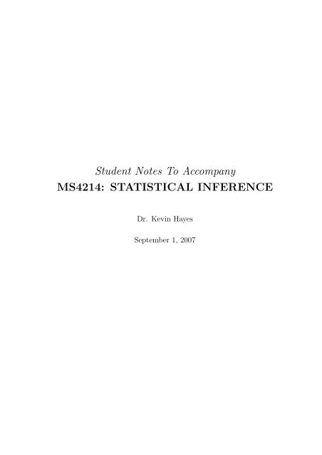
Example 2.4 (Germinating seeds). Suppose 25 seeds were planted and r = 5 seeds
germinated. Then ˆ θ = r/n = 0.2 and Var( ˆ θ) = 0.2 × 0.8/25 = 0.0064. The relative
likelihood is
R1(θ) =
� �5 � �20 θ 1 − θ
.
0.2 0.8
Suppose 100 seeds were planted and r = 20 seeds germinated. Then ˆ θ = r/n = 0.2
but Var( ˆ θ) = 0.2 × 0.8/100 = 0.0016. The relative likelihood is
R2(θ) =
� θ
0.2
� 20 � 1 − θ
0.8
� 80
.
Suppose 25 seeds were planted and it is known only that r ≤ 5 seeds germinated. In
this case the exact number of germinating seeds is unknown. The information about θ
is given by the likelihood function
L (θ) = P (R ≤ 5) =
21
5�
r=0
� �
25
θ
r
r (1 − θ) 25−r .

Relative Likelihood
0.0 0.2 0.4 0.6 0.8 1.0
Germinating probability
0.0 0.1 0.2 0.3 0.4 0.5 0.6 0.7
θ
r = 5 n = 25
r = 20 n = 100
r ≤ 5 n = 25
Figure 2.4.1: Relative likelihood functions for seed germinating probabilities.
Here, the most plausible value for θ is ˆ θ = 0, implying L( ˆ θ) = 1. The relative likelihood
is R3 (θ) = L(θ)/L( ˆ θ) = L(θ). R1 (θ) is plotted as the dashed curve in figure 2.4.1.
R2 (θ) is plotted as the dotted curve in figure 2.4.1. R3 (θ) is plotted as a solid curve
in figure 2.4.1. �
Example 2.5 (Prevalence of a Genotype). Geneticists interested in the prevalence of a
certain genotype, observe that the genotype makes its first appearance in the 22nd sub-
ject analysed. If we assume that the subjects are independent, the likelihood function
can be computed based on the geometric distribution, as L(θ) = (1−θ) n−1 θ. The score
function is then S(θ) = θ −1 −(n−1)(1−θ) −1 . Setting S( ˆ θ) = 0 we get ˆ θ = n −1 = 22 −1 .
The observed Fisher information equals I(θ) = θ −2 + (n − 1)(1 − θ) −2 and is greater
than zero for all θ, implying that ˆ θ is MLE.
Suppose that the geneticists had planned to stop sampling once they observed
r = 10 subjects with the specified genotype, and the tenth subject with the genotype
was the 100th subject anaylsed overall. The likelihood of θ can be computed based on
the negative binomial distribution, as
� �
n − 1
L(θ) = θ
r − 1
r (1 − θ) n−r
for n = 100, r = 5. The usual calculation will confirm that ˆ θ = r/n is MLE. �
22

Example 2.6 (Radioactive Decay). In this classic set of data Rutherford and Geiger
counted the number of scintillations in 72 second intervals caused by radioactive decay
of a quantity of the element polonium. Altogether there were 10097 scintillations during
2608 such intervals:
Count 0 1 2 3 4 5 6 7
Observed 57 203 383 525 532 408 573 139
Count 8 9 10 11 12 13 14
Observed 45 27 10 4 1 0 1
The Poisson probability mass function with mean parameter θ is
The likelihood function equals
fX(x|θ) = θx exp (−θ)
.
x!
L(θ) = � θ xi exp (−θ)
xi!
The relevant mathematical calculations are
= θ� xi exp (−nθ)
� .
xi!
ℓ(θ) = (Σxi) ln (θ) − nθ − ln [Π(xi!)]
S(θ) =
⇒ ˆ θ =
� xi
θ
� xi
n
− n
= ¯x
I(θ) = Σxi
> 0,
θ2 ∀ θ
implying ˆ θ is MLE. Also E( ˆ θ) = � E(xi) = 1 �
θ = θ, so θˆ is an unbiased estimator.
� Var(xi) = 1
Next Var( ˆ θ) = 1
n2 nθ and I(θ) = E[I(θ)] = n/θ = (Var[ˆ θ]) −1 implying
that ˆ θ attains the theoretical CRLB. It is always useful to compare the fitted values
from a model against the observed values.
i 0 1 2 3 4 5 6 7 8 9 10 11 12 13 14
Oi 57 203 383 525 532 408 573 139 45 27 10 4 1 0 1
Ei 54 211 407 525 508 393 254 140 68 29 11 4 1 0 0
n
+3 -8 -24 0 +24 +15 +19 -1 -23 -2 -1 0 -1 +1 +1
The Poisson law agrees with the observed variation within about one-twentieth of its
range. �
23

Example 2.7 (Exponential distribution). Suppose random variables X1, . . . , Xn are i.i.d.
as Exp(θ). Then
L(θ) =
n�
θ exp (−θxi)
i=1
= θ n exp
�
−θ � �
xi
ℓ(θ) = n ln θ − θ � xi
S(θ) = n
θ −
⇒ θ ˆ
I(θ)
=
=
n�
xi
i=1
n
�
xi
n
> 0
θ2 ∀ θ.
In order to work out the expectation and variance of ˆ θ we need to work out the
probability distribution of Z = n�
Xi, where Xi ∼ Exp(θ). From the appendix on
i=1
probability theory we have Z ∼ Ga(θ, n). Then
� �
1
E
Z
We now return to our estimator
implies
=
�∞
0
1
z
= θ2
Γ(n)
=
= θ Γ(n − 1)
E[ ˆ θ] = E
θ
Γ(n)
θnzn−1 exp (−θz)
dz
Γ(n)
�
∞
0
∞
�
0
Γ(n)
ˆθ = n
n�
xi
i=1
(θz) n−2 exp (−θz)dz
u n−2 exp (−u)du
= θ
n − 1 .
= n
Z
�
n
� � �
1
= nE =
Z Z
n
n − 1 θ
which turns out to be biased. Propose the alternative estimator ˜ θ = n−1
n ˆ θ. Then
E[ ˜ �
(n − 1)
θ] = E
n
�
ˆθ = (n − 1)
shows ˜ θ is an unbiased estimator.
E[
n
ˆ θ] =
24
(n − 1)
n
� �
n
θ = θ
n − 1

As this example demonstrates, maximum likelihood estimation does not automati-
cally produce unbiased estimates. If it is thought that this property is (in some sense)
desirable, then some adjustments to the MLEs, usually in the form of scaling, may be
required. We conclude this example with the following tedious (but straightforward)
calculations.
�
1
E
Z2 �
We have already calculated that
However,
�∞
1
= θ
Γ(n)
0
n z n−3 exp −θzdz
= θ2
�∞
u
Γ(n)
n−3 exp −θudu
0
= θ2 Γ(n − 2)
Γ(n)
=
θ 2
(n − 1)(n − 2)
⇒ Var[ ˜ θ] = E[ ˜ θ 2 �
] − E[ ˜ � �
2
2 (n − 1)
θ] = E
Z2 �
− θ 2
=
(n − 1) 2θ2 (n − 1)(n − 2) − θ2 = θ2
n − 2 .
I(θ) = n
θ2 ⇒ E [I(θ)] = n
θ
eff( ˜ θ) =
(E [I(θ)])−1
Var[ ˜ θ]
2 �=
θ2 θ2
= ÷
n n − 2
�
Var[ ˜ �−1 θ] .
= n − 2
n
which although not equal to 1, converges to 1 as n → ∞, and ˜ θ is asymptotically
efficient. �
Example 2.8 (Lifetime of a component). The time to failure T of components has an
exponential distributed with mean µ. Suppose n components are tested for 100 hours
and that m components failed at times t1, . . . , tm, with n − m components surviving
the 100 hour test. The likelihood function can be written
m� 1
L(θ) =
µ
i=1
e−ti/µ
n�
P (Tj > 100) .
j=m+1
� �� � � �� �
components failed components survived
Clearly P (T ≤ t) = 1 − e −t/µ implies P (T > 100) = e −100/µ is the probability of a
component surviving the 100 hour test. Then
L(µ) =
�
m�
1
µ e−ti/µ
�
�e−100/µ �n−m
,
i=1
25

ℓ(µ) = −m ln µ − 1
m�
ti −
µ
i=1
1
µ 100(n − m),
S(µ) = − m
µ + 1
µ 2
m�
ti + 1
µ 2 100(n − m).
Setting S(ˆµ) = 0 suggests the estimator ˆµ = [ � m
i=1 ti + 100 (n − m)] /m. Also, I(ˆµ) =
m/ˆµ 2 > 0, and ˆµ is indeed the MLE. Although failure times were recorded for just m
components, this example usefully demonstrates that all n components contribute to
the estimation of the mean failure parameter µ. The n − m surviving components are
often referred to as right censored. �
i=1
Example 2.9 (Gaussian Distribution). Consider data X1, X2 . . . , Xn distributed as N(µ, υ).
Then the likelihood function is
L(µ, υ) =
and the log-likelihood function is
⎧
� �n ⎪⎨
1
√πυ exp −
⎪⎩
n�
(xi − µ) 2
⎫
⎪⎬
i=1
ℓ(µ, υ) = − n n 1
ln (2π) − ln (υ) −
2 2 2υ
2υ
⎪⎭
n�
(xi − µ) 2
i=1
(2.3)
Unknown mean and known variance: As υ is known we treat this parameter as a con-
stant when differentiating wrt µ. Then
S(µ) = 1
υ
n�
i=1
(xi − µ), ˆµ = 1
n
n�
i=1
xi, and I(θ) = n
υ
Also, E[ˆµ] = nµ/n = µ, and so the MLE of µ is unbiased. Finally
Var[ˆµ] = 1
�
n�
�
Var xi =
n2 υ
n = (E[I(θ)])−1 .
Known mean and unknown variance: Differentiating (2.3) wrt υ returns
and setting S(υ) = 0 implies
i=1
S(υ) = − n 1
+
2υ 2υ2 ˆυ = 1
n
n�
(xi − µ) 2 ,
i=1
n�
(xi − µ) 2 .
i=1
26
> 0 ∀ µ.

Differentiating again, and multiplying by −1 yields the information function
Clearly ˆυ is the MLE since
Define
I(υ) = − n 1
+
2υ2 υ3 n�
(xi − µ) 2 .
i=1
I(ˆυ) = n
> 0.
2υ2 Zi = (Xi − µ) 2 / √ υ,
so that Zi ∼ N(0, 1). From the appendix on probability
n�
Z 2 i ∼ χ 2 n,
implying E[ � Z 2 i ] = n, and Var[ � Z 2 i ] = 2n. The MLE
Then
and
Finally,
Var[ˆυ] =
i=1
ˆυ = (υ/n)
E[ˆυ] = E
�
υ
n
n�
i=1
n�
i=1
Z 2 i
Z 2 i .
�
= υ,
�
�
υ
� n�
2
Var Z
n
i=1
2 �
i = 2υ2
n .
E [I(υ)] = − n 1
+
2υ2 υ3 = − n nυ
+
2υ2 υ3 = n
.
2υ2 n�
E � (xi − µ) 2�
Hence the CRLB = 2υ 2 /n, and so ˆυ has efficiency 1. �
Our treatment of the two parameters of the Gaussian distribution in the last ex-
ample was to (i) fix the variance and estimate the mean using maximum likelihood;
and then (ii) fix the mean and estimate the variance using maximum likelihood. In
practice we would like to consider the simultaneous estimation of these parameters. In
the next section of these notes we extend MLE to multiple parameter estimation.
27
i=1

2.5 Multi-parameter Estimation
Suppose that a statistical model specifies that the data y has a probability distribution
f(y; α, β) depending on two unknown parameters α and β. In this case the likelihood
function is a function of the two variables α and β and having observed the value y is
defined as L(α, β) = f(y; α, β) with ℓ(α, β) = ln L(α, β). The MLE of (α, β) is a value
(ˆα, ˆ β) for which L(α, β) , or equivalently ℓ(α, β) , attains its maximum value.
Define S1(α, β) = ∂ℓ/∂α and S2(α, β) = ∂ℓ/∂β. The MLEs (ˆα, ˆ β) can be obtained
by solving the pair of simultaneous equations :
S1(α, β) = 0
S2(α, β) = 0
The information matrix I(α, β) is defined to be the matrix :
�
I11(α, β)
I(α, β) =
I21(α, β)
� �
I12(α, β)
= −
I22(α, β)
∂2 ∂α2 ℓ ∂2 ∂α∂β ℓ
∂2 ∂β∂α ℓ ∂2 ∂β2 ℓ
The conditions for a value (α0, β0) satisfying S1(α0, β0) = 0 and S2(α0, β0) = 0 to
be a MLE are that
and
I11(α0, β0) > 0, I22(α0, β0) > 0,
det(I(α0, β0) = I11(α0, β0)I22(α0, β0) − I12(α0, β0) 2 > 0.
This is equivalent to requiring that both eigenvalues of the matrix I(α0, β0) be positive.
Example 2.10 (Gaussian distribution). Let X1, X2 . . . , Xn be iid observations from a
N (µ, v) density in which both µ and v are unknown. The log likelihood is
ℓ(µ, v) =
n�
�
1
ln √ exp [−
2πv i=1
1
2v (xi − µ) 2 =
�
]
n�
�
−
i=1
1 1 1
ln [2π] − ln [v] −
2 2 2v (xi − µ) 2
�
= − n
n�
n 1
ln [2π] − ln [v] − (xi − µ)
2 2 2v
2 .
Hence
implies that
S1(µ, v) = ∂ℓ
∂µ
ˆµ = 1
n
= 1
v
i=1
n�
(xi − µ) = 0
i=1
n�
xi = ¯x. (2.4)
i=1
28
�

Also
implies that
S2(µ, v) = ∂ℓ
∂v
ˆv = 1
n
n�
i=1
n 1
= − +
2v 2v2 (xi − ˆµ) 2 = 1
n
n�
(xi − µ) 2 = 0
i=1
n�
(xi − ¯x) 2 . (2.5)
Calculating second derivatives and multiplying by −1 gives that the information matrix
I(µ, v) equals
I(µ, v) =
⎛
⎜
⎝
1
v 2
i=1
i=1
n
1
v
v2 n�
(xi − µ)
i=1
n�
(xi − µ) − n
2v2 + 1
v3 n�
(xi − µ) 2
⎞
⎟
⎠
Hence I(ˆµ, ˆv) is given by : �
n
ˆv 0
0 n
2v2 �
Clearly both diagonal terms are positive and the determinant is positive and so (ˆµ, ˆv)
are, indeed, the MLEs of (µ, v).
Go back to equation (2.4), and ¯ X ∼ N (µ, v/n). Clearly E( ¯ X) = µ (unbiased) and
Var( ¯ X) = v/n, so ¯ X achieved the CRLB. Go back to equation (2.5). Then from lemma
2.9 we have
so that
nˆv
v ∼ χ2 n−1
i=1
� �
nˆv
E = n − 1
v
� �
n − 1
⇒ E(ˆv) = v
n
Instead, propose the (unbiased) estimator
Observe that
E(˜v) =
˜v =
n
ˆv =
n − 1
� �
n
E(ˆv) =
n − 1
1
n − 1
n�
(xi − ¯x) 2
i=1
� n
n − 1
� � n − 1
and ˜v is unbiased as suggested. We can easily show that
Hence
Var(˜v) =
2v 2
(n − 1)
n
�
v = v
(2.6)
eff(˜v) = 2v2 2v2 1
÷ = 1 −
n (n − 1) n
Clearly ˜v is not efficient, but is asymptotically efficient. �
29

Lemma 2.9 (Joint distribution of the sample mean and sample variance). If
X1, . . . , Xn are iid N (µ, v) then the sample mean ¯ X and sample variance S 2 /(n − 1)
are independent. Also ¯ X is distributed N (µ, v/n) and S 2 /v is a chi-squared random
variable with n − 1 degrees of freedom.
Proof. Define
⇒
W =
n�
(Xi − ¯ X) 2 =
i=1
W
v + ( ¯ X − µ) 2
v/n
=
n�
(Xi − µ) 2 − n( ¯ X − µ) 2
i=1
n� (Xi − µ) 2
The RHS is the sum of n independent standard normal random variables squared, and
so is distributed χ 2 ndf Also, ¯ X ∼ N (µ, v/n), therefore ( ¯ X − µ) 2 /(v/n) is the square of
a standard normal and so is distributed χ2 1df These Chi-Squared random variables have
moment generating functions (1 − 2t) −n/2 and (1 − 2t) −1/2 respectively. Next, W/v and
( ¯ X − µ) 2 /(v/n) are independent:
Cov(Xi − ¯ X, ¯ X) = Cov(Xi, ¯ X) − Cov( ¯ X, ¯ X)
�
= Cov Xi, 1 �
�
Xj − Var(
n
¯ X)
= 1 �
Cov(Xi, Xj) −
n
v
n
j
= v v
−
n n
i=1
= 0
But, Cov(Xi − ¯ X, ¯ X − µ) = Cov(Xi − ¯ X, ¯ X) = 0 , hence
�
Cov(Xi − ¯ X, ¯ �
�
X − µ) = Cov (Xi − ¯ X), ¯ �
X − µ = 0
i
As the moment generating function of the sum of independent random variables is
equal to the product of their individual moment generating functions, we see
E � e t(W/v)� (1 − 2t) −1/2 = (1 − 2t) −n/2
⇒ E � e t(W/v)� = (1 − 2t) −(n−1)/2
But (1 − 2t) −(n−1)/2 is the moment generating function of a χ 2 random variables with
(n−1) degrees of freedom, and the moment generating function uniquely characterizes
the random variable S = (W/v).
30
i
v

Suppose that a statistical model specifies that the data x has a probability distribu-
tion f(x; θ) depending on a vector of m unknown parameters θ = (θ1, . . . , θm). In this
case the likelihood function is a function of the m parameters θ1, . . . , θm and having
observed the value of x is defined as L(θ) = f(x; θ) with ℓ(θ) = ln L(θ).
The MLE of θ is a value ˆ θ for which L(θ), or equivalently ℓ(θ), attains its maximum
value. For r = 1, . . . , m define Sr(θ) = ∂ℓ/∂θr. Then we can (usually) find the MLE
ˆθ by solving the set of m simultaneous equations Sr(θ) = 0 for r = 1, . . . , m. The
information matrix I(θ) is defined to be the m×m matrix whose (r, s) element is given
by Irs where Irs = −∂ 2 ℓ/∂θr∂θs. The conditions for a value ˆ θ satisfying Sr( ˆ θ) = 0 for
r = 1, . . . , m to be a MLE are that all the eigenvalues of the matrix I( ˆ θ) are positive.
2.6 Newton-Raphsom Optimization
Example 2.11 (Radioactive Scatter). A radioactive source emits particles intermittently
and at various angles. Let X denote the cosine of the angle of emission. The angle
of emission can range from 0 degrees to 180 degrees and so X takes values in [−1, 1].
Assume that X has density
1 + θx
f(x|θ) =
2
for −1 ≤ x ≤ 1 where θ ∈ [−1, 1] is unknown. Suppose the data consist of n indepen-
dently identically distributed measures of X yielding values x1, x2, ..., xn. Here
L(θ) = 1
2 n
n�
(1 + θxi)
i=1
l(θ) = −n ln [2] +
S(θ) =
I(θ) =
n�
i=1
n�
i=1
xi
1 + θxi
n�
ln [1 + θxi]
i=1
x 2 i
(1 + θxi) 2
Since I(θ) > 0 for all θ, the MLE may be found by solving the equation S(θ) = 0. It
is not immediately obvious how to solve this equation.
By Taylor’s Theorem we have
0 = S( ˆ θ)
= S(θ0) + ( ˆ θ − θ0)S ′ (θ0) + ( ˆ θ − θ0) 2 S ′′ (θ0)/2 + ....
31

So, if | ˆ θ − θ0| is small, we have that
and hence
0 ≈ S(θ0) + ( ˆ θ − θ0)S ′ (θ0),
ˆθ ≈ θ0 − S(θ0)/S ′ (θ0)
= θ0 + S(θ0)/I(θ0)
We now replace θ0 by this improved approximation θ0 +S(θ0)/I(θ0) and keep repeating
the process until we find a value ˆ θ for which |S( ˆ θ)| < ɛ where ɛ is some prechosen small
number such as 0.000001. This method is called Newton’s method for solving a nonlinear
equation.
If a unique solution to S(θ) = 0 exists, Newton’s method works well regardless of
the choice of θ0. When there are multiple solutions, the solution to which the algorithm
converges depends crucially on the choice of θ0. In many instances it is a good idea
to try various starting values just to be sure that the method is not sensitive to the
choice of θ0.
One approach to finding an initial estimate θ0 would be to use the Method of
Moments. This involves solving the equation E(X) = ¯x for θ. For the previous example
E(X) =
� 1
−1
x(1 + θx)
dx =
2
θ
3
and so θ0 = 3¯x might yield a good choice for a starting value.
Suppose the following 10 values were recorded:
0.00, 0.23, −0.05, 0.01, −0.89, 0.19, 0.28, 0.51, −0.25 and 0.27.
Then ¯x = 0.03, and we substitute θ0 = .09 into the updating formula
ˆθnew = θ old +
� n�
⇒ θ1 = 0.2160061
θ2 = 0.2005475
θ3 = 0.2003788
θ4 = 0.2003788
i=1
xi
1 + θ old xi
� � n�
i=1
x 2 i
(1 + θ old xi) 2
The relative likelihood function is plotted in Figure 2.6.2. �
32
� −1

Relative Likelihood
0.4 0.6 0.8 1.0
Radioactive Scatter
−1.0 −0.5 0.0 0.5 1.0
θ
θ ^ = 0.2003788
Figure 2.6.2: Relative likelihood for the radioactive scatter, solved by Newton Raphson.
A Weibull random variable with ‘shape’ parameter a > 0 and ‘scale’ parameter
b > 0 has density
fT (t) = (a/b)(t/b) a−1 exp{−(t/b) a }
for t ≥ 0. The (cumulative) distribution function is
FT (t) = 1 − exp{−(t/b) a }
on t ≥ 0. Suppose that the time to failure T of components has a Weibull distribution
and after testing n components for 100 hours, m components fail at times t1, . . . , tm,
with n − m components surviving the 100 hour test. The likelihood function can be
written
L(θ) =
m�
� �a−1 � � �a� a ti
ti
exp −
b b
b
i=1
� �� �
components failed
33
n�
� � �a� 100
exp − .
b
j=m+1
� �� �
components survived

Then the log-likelihood function is
ℓ(a, b) = m ln (a) − ma ln (b) + (a − 1)
m�
ln (ti) −
i=1
n�
(ti/b) a ,
where for convenience we have written tm+1 = · · · = tn = 100. This yields score
functions
and
Sa(a, b) = m
a
− m ln (b) +
m�
ln (ti) −
i=1
Sb(a, b) = − ma
b
+ a
b
i=1
n�
(ti/b) a ln (ti/b) ,
It is not obvious how to solve Sa(a, b) = Sb(a, b) = 0 for a and b.
i=1
n�
(ti/b) a . (2.7)
When the m equations Sr(θ) = 0, r = 1, . . . , m cannot be solved directly numerical
optimization is required. Let S(θ) be the m × 1 vector whose rth element is Sr(θ). Let
ˆθ be the solution to the set of equations S(θ) = 0 and let θ0 be an initial guess at ˆ θ.
Then a first order Taylor’s series approximation to the function S about the point θ0
is given by
Sr( ˆ m�
θ) ≈ Sr(θ0) + ( ˆ θj − θ0j) ∂Sr
(θ0)
∂θj
for r = 1, 2, . . . , m which may be written in matrix notation as
j=1
i=1
S( ˆ θ) ≈ S(θ0) − I(θ0)( ˆ θ − θ0).
Requiring S( ˆ θ) = 0, this last equation can be reorganized to give
ˆθ ≈ θ0 + I(θ0) −1 S(θ0). (2.8)
Thus given θ0 this is a method for finding an improved guess at ˆ θ. We then replace θ0
by this improved guess and repeat the process. We keep repeating the process until we
obtain a value θ ∗ for which |Sr(θ ∗ )| is less than ɛ for r = 1, 2, . . . , m where ɛ is some
small number like 0.0001. θ ∗ will be an approximate solution to the set of equations
S(θ) = 0. We then evaluate the matrix I(θ ∗ ) and if all m of its eigenvalues are positive
we set ˆ θ = θ ∗ .
For the Weibull distribution
Iaa = m
+
a2 n�
i=1
Ibb = − ma a(a + 1)
+
b2 b2 Iab = Iba = m
b
(ti/b) a [ln (ti/b)] 2 ,
− 1
b
n�
(ti/b) a ,
i=1
n�
(ti/b) a [a ln (ti/b) + 1] .
i=1
34

a0 b0 a ∗ b ∗ Steps Eigenvalues
1.8 74.5 1.924941 78.12213 4 all positive
2.36 72 1.924941 78.12213 5 all positive
2 70 1.924941 78.12213 5 all positive
1 2 1.924941 78.12213 15 all positive
80 1 1.924941 78.12213 387 all positive
2 100 4.292059 −34.591322 2 crashed
Table 2.6.1: Newton-Raphson estimates of the Weibull parameters.
Given initial values a0 and b0 equation (2.8) can be used to obtained updated estimates
via
�
anew
bnew
�
=
�
a0
b0
�
+
�
Iaa(a0, b0) Iab(a0, b0)
Iba(a0, b0) Ibb(a0, b0)
� −1 �
Sa(a0, b0)
Sb(a0, b0)
�
. (2.9)
Having solved for a and b we check that a maximum has been achieved by calculating
I(a ∗ , b ∗ ) and verifying that both of its eigenvalues are positive.
Suppose n = 10 and m = 8 items fail at times 17, 29, 32, 55, 61, 74, 77, 93 (in hours)
with the remaining two items surviving the 100 hour test. Table 2.6.1 shows estimates
(a ∗ , b ∗ ) obtained from equation (2.9) using various starting values (a0, b0) along with
the number of iteration steps taken until convergence using ɛ = 0.000001. Four of
the starting pairs considered converged to estimates a ∗ = 1.924941 and b ∗ = 78.12213
for a and b. The starting pairs (1, 2) and (80, 1) might misleadingly suggest that the
algorithm is robust to the choice of starting values. However, the starting pair (2, 100)
produced a negative estimate of b, and as ln(b) is required in the computation of the
score function, caused the algorithm to crash. Other starting pairs not reported failed
to yield estimates due to a non-invertible I(θ0) matrix being produced during the
running of the algorithm. The remainder of this section describes commonly applied
modifications of the Newton-Raphson method.
Initial values
The Newton-Raphson method depends on the initial guess being close to the true value.
If this requirement is not satisfied the procedure might convergence to a minimum
instead of a maximum, or just simply diverge and fail to produce any estimates at all.
Methods of finding good initial estimates depend very much on the problem at hand
and may require some ingenuity.
The distribution function of a Weibull random variable T can be linearized as
ln(− ln[1 − F (t)]) = −a ln(b) + a ln(t).
35

A regression of the empirical distribution function ˆ F (t) on ln(t) can be used the recover
initial estimates for a and b. The starting pair (1.8, 74.5) in Table 2.6.1 was obtained
in this way.
A more general method for finding initial values is the method of moments. This
method estimates the kth moment about the origin E(T k ) by the sample moment
˜mk = n −1 � t k i . For a Weibull distribution the kth moment about the origin equals
b k Γ(1 + k/a) where Γ(c) = � ∞
0 uc−1 e −u du is the usual gamma function satisfying
Γ(c) = (c − 1)Γ(c − 1). It is easy to show that E(T 2 )/[E(T )] 2 = 2aΓ(2/a)/[Γ(1/a)] 2 . An
estimate a0 of a can be obtained by solving ˜m 2 2/( ˜m1) 2 = 2aΓ(2/a)/[Γ(1/a)] 2 for a. The
corresponding estimate of b is then b0 = ˜m1/Γ(1 + 1/a0). The starting pair (2.36, 72)
in Table 2.6.1 was obtained in this way.
Fisher’s method of scoring
One modification to Newton’s method is to replace the matrix I(θ) in (2.8) with Ī(θ) =
E [I(θ)] . The matrix Ī(θ) is positive definite, thus overcoming many of the problems
regarding matrix inversion. Like Newton-Raphson, there is no guarantee that Fisher’s
method of scoring will avoid producing negative parameter estimates or converging to
local minima. Unfortunately, calculating Ī(θ) often can be mathematically difficult.
The profile likelihood
Setting Sb(a, b) = 0 from equation (2.7) we can solve for b in terms of a as
�
1
b =
m
n�
i=1
t a i
� 1/a
. (2.10)
This reduces our two parameter problem to a search over the “new” one-parameter
profile log-likelihood
ℓa(a) = ℓ(a, b(a)),
�
= m ln (a) − m ln
1
m
n�
i=1
t a i
�
+ (a − 1)
m�
ln (ti) − m. (2.11)
Given an initial guess a0 for a, an improved estimate a1 can be obtained using a
single parameter Newton-Raphson updating step a1 = a0 + S(a0)/I(a0), where S(a)
and I(a) are now obtained from ℓa(a). The estimates â = 1.924941 and ˆ b = 78.12213
were obtained by applying this method to the Weibull data using starting values a0 =
0.001 and a0 = 5.8 in 16 and 13 iterations respectively. However, the starting value
a0 = 5.9 produced the sequence of estimates a1 = −5.544163, a2 = 8.013465, a3 =
−16.02908, a4 = 230.0001 and subsequently crashed.
36
i=1

Reparameterization
Negative parameter estimates can be avoided by reparameterizing the profile log-
likelihood in (2.11) using α = ln(a). Since a = e α we are guaranteed to obtain a > 0.
The reparameterized profile log-likelihood becomes
�
n� 1
ℓα(α) = mα − m ln t
m
eα
�
i + (e α − 1)
implying score function
and information function
I(α) =
i=1
S(α) = m − meα � n
meα �n i=1 teα i
i=1 teα
�n i=1 teα i
�
n�
t eα
i ln(ti) − e α [� n
i=1
i ln(ti)
+ e α
+e α
m�
ln (ti) − m,
i=1
m�
ln(ti)
i=1
i=1 teα i ln(ti)] 2
�n i=1 teα i
n�
i=1
t eα
i [ln(ti)] 2
�
− e α
m�
ln(ti).
The estimates â = 1.924941 and ˆ b = 78.12213 were obtained by applying this method
to the Weibull data using starting values a0 = 0.07 and a0 = 76 in 103 and 105
iterations respectively. However, the starting values a0 = 0.06 and a0 = 77 failed due
to division by computationally tiny (1.0e-300) values.
The step-halving scheme
The Newton-Raphson method uses the (first and second) derivatives of ℓ(θ) to max-
imize the function ℓ(θ), but the function itself is not used in the algorithm. The
log-likelihood can be incorporated into the Newton-Raphson method by modifying the
updating step to
θi+1 = θi + λiI(θi) −1 S(θi), (2.12)
where the search direction has been multiplied by some λi ∈ (0, 1] chosen so that the
inequality
ℓ � θi + λiI(θi) −1 S(θi) � > ℓ (θi) (2.13)
holds. This requirement protects the algorithm from converging towards minima or
saddle points. At each iteration the algorithm sets λi = 1, and if (2.13) does not
hold λi is replaced with λi/2. The process is repeated until the inequality in (2.13) is
satisfied. At this point the parameter estimates are updated using (2.12) with the value
of λi for which (2.13) holds. If the function ℓ(θ) is concave and unimodal convergence
is guaranteed. Finally, when
maxima is guaranteed, even if ℓ(θ) is not concave.
Ī(θ) is used in place of I(θ) convergence to a (local)
37
i=1

2.7 The Invariance Principle
How do we deal with parameter transformation? We will assume a one-to-one trans-
formation, but the idea applied generally. Consider a binomial sample with n = 10
independent trials resulting in data x = 8 successes. The likelihood ratio of θ1 = 0.8
versus θ2 = 0.3 is
L(θ1 = 0.8)
L(θ2 = 0.3) = θ8 1(1 − θ1) 2
θ8 = 208.7 ,
2(1 − θ2) 2
that is, given the data θ = 0.8 is about 200 times more likely than θ = 0.3.
Suppose we are interested in expressing θ on the logit scale as
ψ ≡ ln{θ/(1 − θ)} ,
then ‘intuitively’ our relative information about ψ1 = ln(0.8/0.2) = 1.29 versus ψ2 =
ln(0.3/0.7) = −0.85 should be
L ∗ (ψ1)
L ∗ (ψ2)
= L(θ1)
L(θ2)
= 208.7 .
That is, our information should be invariant to the choice of parameterization. ( For
the purposes of this example we are not too concerned about how to calculate L ∗ (ψ). )
Theorem 2.10 (Invariance of the MLE). If g is a one-to-one function, and ˆ θ is
the MLE of θ then g( ˆ θ) is the MLE of g(θ).
Proof. This is trivially true as we let θ = g −1 (µ) then f{y|g −1 (µ)} is maximized in µ
exactly when µ = g( ˆ θ). When g is not one-to-one the discussion becomes more subtle,
but we simply choose to define ˆgMLE(θ) = g( ˆ θ)
It seems intuitive that if ˆ θ is most likely for θ and our knowledge (data) remains
unchanged then g( ˆ θ) is most likely for g(θ). In fact, we would find it strange if ˆ θ is an
estimate of θ, but ˆ θ 2 is not an estimate of θ 2 . In the binomial example with n = 10
and x = 8 we get ˆ θ = 0.8, so the MLE of g(θ) = θ/(1 − θ) is
g( ˆ θ) = ˆ θ/(1 − ˆ θ) = 0.8/0.2 = 4.
This convenient property is not necessarily true of other estimators. For example, if ˆ θ
is the MVUE of θ, then g( ˆ θ) is generally not MVUE for g(θ).
Frequentists generally accept the invariance principle without question. This is
not the case for intelligent lifeforms such as Bayesians. The invariance property of
the likeihood ratio is incompatible with the Bayesian habit of assigning a probability
distribution to a parameter.
38

2.8 Optimality Properties of the MLE
Suppose that an experiment consists of measuring random variables x1, x2, . . . , xn which
are iid with probability distribution depending on a parameter θ. Let ˆ θ be the MLE
of θ. Define
W1 = � E[I(θ)]( ˆ θ − θ)
W2 = � I(θ)( ˆ θ − θ)
�
W3 = E[I( ˆ θ)]( ˆ θ − θ)
�
W4 = I( ˆ θ)( ˆ θ − θ).
Then, W1, W2, W3, and W4 are all random variables and, as n → ∞, the probabilistic
behaviour of each of W1, W2, W3, and W4 is well approximated by that of a N(0, 1)
random variable. Then, since E[W1] ≈ 0, we have that E[ ˆ θ] ≈ θ and so ˆ θ is approx-
imately unbiased. Also Var[W1] ≈ 1 implies that Var[ ˆ θ] ≈ (E[I(θ)]) −1 and so ˆ θ is
approximately efficient.
Let the data X have probability distribution g(X; θ) where θ = (θ1, θ2, . . . , θm) is a
vector of m unknown parameters. Let I(θ) be the m×m information matrix as defined
above and let E[I(θ)] be the m × m matrix obtained by replacing the elements of I(θ)
by their expected values. Let ˆ θ be the MLE of θ. Let CRLBr be the rth diagonal
element of [E[I(θ)]] −1 . For r = 1, 2, . . . , m, define W1r = ( ˆ θr − θr)/ √ CRLBr. Then, as
n → ∞, W1r behaves like a standard normal random variable.
Suppose we define W2r by replacing CRLBr by the rth diagonal element of the
matrix [I(θ)] −1 , W3r by replacing CRLBr by the rth diagonal element of the matrix
[EI( ˆ θ)] −1 and W4r by replacing CRLBr by the rth diagonal element of the matrix
[I( ˆ θ)] −1 . Then it can be shown that as n → ∞, W2r, W3r, and W4r all behave like
standard normal random variables.
2.9 Data Reduction
Definition 2.11 (Sufficiency). Consider a statistic T = t(X) that summarises the
data so that no information about θ is lost. Then we call t(X) a sufficient statistic. �
Example 2.12. T = t(X) = ¯ X is sufficient for µ when Xi ∼ iid N(µ, σ 2 ). �
To better understand the motivation behind the concept of sufficiency consider
three independent Binomial trials where θ = P (X = 1).
39

Event Probability Set
0 0 0 (1 − θ) 3 A0
1 0 0
0 1 0
0 0 1
0 1 1
1 0 1
1 1 0
θ(1 − θ) 2 A1
θ 2 (1 − θ) A2
1 1 1 θ 3 A4
Knowing which Ai the sample is in carries all the information about θ. Which
particular sample within Ai gives us no extra information about θ. Extra information
about other aspect of the model maybe, but not about θ. Here T = t(X) = � Xi
equals the number of “successes”, and identifies Ai. Mathematically we can express
the above concept by saying that the probability P (X = x|Ai) does not depend on θ.
i.e. P (010|A1; θ) = 1/3. More generally, a statistic T = t(X) is said to be sufficient
for the parameter θ if Pr (X = x|T = t) does not depend on θ. Sufficient statistics are
most easily recognized through the following fundamental result:
Theorem 2.11 (Neyman’s Factorization Criterion). A statistic T = t(X) is
sufficient for θ if and only if the family of densities can be factorized as
f(x; θ) = h(x)k {t(x); θ} , x ∈ X , θ ∈ Θ. (2.14)
i.e. into a function which does not depend on θ and one which only depends on x
through t(x). This is true in general. We will prove it in the case where X is discrete.
Proof. Assume T is sufficient and let h(x) = Pθ {X = x|T = t(x)} be independent of
θ. Let k {t; θ} = Pθ(T = t). Then
f(x; θ) = Pθ {X = x|T = t(x)} Pθ {T = t(x)} = h(x)k {θ, t(x)} .
Conversely assume the result in (2.14) to be true. Then
Pθ (X = x|T = t) =
which is independent of θ.
=
=
h(x)k {t(x); θ}
1{x:t(x)=t}(x),
h(y)k {t(y); θ}
�
y:t(y)=t
h(x)k {t; θ}
k {t; θ} �
1{x:t(x)=t}(x),
y:t(y)=t h(y)
h(x)
�
y:t(y)=t
40
h(y) 1{x:t(x)=t}(x),

Example 2.13 (Poisson). Let X = (X1, . . . , Xn) be independent and Poisson dis-
tributed with mean λ so that
f(x; λ) =
n�
i=1
λxi xi! e−λ = λΣxi
�
i xi! e−nλ .
Take k { � xi; λ} = λ Σxi e −nλ and h(x) = ( � xi!) −1 , then t(x) = �
i xi is sufficient. �
Example 2.14 (Binomial). Let X = (X1, . . . , Xn) be independent and Bernoulli dis-
tributed with parameter θ so that
f(x; θ) =
n�
θ xi 1−xi Σxi n−Σxi
(1 − θ) = θ (1 − θ)
i=1
Take k { � xi; θ} = θ Σxi (1 − θ) n−Σxi and h(x) = 1, then t(x) = �
i xi is sufficient. �
Example 2.15 (Uniform). Factorization criterion works in general but can mess up if
the pdf depends on θ. Let X = (X1, . . . , Xn) be independent and Uniform distributed
with parameter θ so that X1, X2, . . . , Xn ∼ Unif(0, θ). Then
f(x; θ) = 1
θ n
0 ≤ xi ≤ θ ∀ i.
It is not at all obvious but t(x) = max(xi) is a sufficient statistic. We have to show
that f(x|t) is independent of θ. Well
Then
So
f(x|t) =
f(x, t)
fT (t) .
P (T ≤ t) = P (X1 ≤ t, . . . , Xn ≤ t)
n�
�
t
= P (Xi ≤ t) =
θ
i=1
FT (t) = tn
θn ⇒ fT (t) = ntn−1
θn Also
f(x, t) = 1
θn ≡ f(x; θ).
Hence
f(x|t) =
1
,
ntn−1 and is independent of θ. �
41
� n

2.10 Worked Problems
The Problems
1. The continuous random variable T has probability density function
f(t) = λe −λt , t > 0; λ > 0.
(a) Show that the cumulative distribution function is given by
(b) Deduce that
F (t) = 1 − e −λt , t > 0; λ > 0.
P (a ≤ b) = e −λa − e −λb , 0 < a < b.
(c) The accounts manager for a building society firm assumes that the time T
taken to settle invoices is a random variable with the pdf f(t) given above
for some unknown value of λ. For a random sample of 100 invoices, he finds
that 50 are settled within one week, 35 are settled during the second week
and 15 are settles after 2 weeks. Explain clearly why the likelihood function
of these data may be written as
where k is a constant.
L(λ) = k(1 − e −λ ) 50 � e −λ e −2λ� 35 (1 − e −2λ ) 15 ,
(d) Show that the maximum likelihood estimate ˆ λ of λ is approximately 0.836.
(e) Using ˆ λ = 0.836, calculate the expected number of invoices settled within
the first week, settled during the second week, and settled after 2 weeks.
Hence comment briefly on how well the model fits the data.
2. A finite population has nA individuals of type A and nB individuals of type
B. The overall number is known to be 100, but the size of the two groups is
unknown. If a sample of 5 individuals is taken without replacement, write down
the likelihood for nA in the following three situations:
(a) the observed sequence is A, B, A, B, A ;
(b) the observed sequence is A, A, B, B, A ;
(c) the precise sequence of the outcomes is not given, but it is known that three
elements are As, two are Bs.
Compare the likelihood functions and comment on your findings.
42

3. A certain type of plant cell may appear in any one of four versions. According to
a genetic theory, the four versions have the following probabilities of appearance:
1/2 + θ/4, (1 − θ)/4, (1 − θ)/4, θ/4,
where θ is a parameter not specified by the genetic theory (0 < θ < 1). If a
sample of n cells had observed frequencies (a, b, c, d) where n = a + b + c + d, find
the maximum likelihood estimate of θ, and an estimate of Var( ˆ θ).
4. Let X1, X2, . . . , Xn be a random sample from a population with probability den-
sity
f(x) =
(a) Show that E(X 2 ) = θ.
�
2
πθ exp
�
− x2
�
, x > 0.
2θ
(b) Find the maximum likelihood estimator (MLE), ˆ θ, of θ.
(c) Show that ˆ θ is an unbiased estimator of θ and that the Cramér-Rao lower
bound is attained. [You may assume Var(X 2 ) = 2θ 2 .]
(d) Suppose now that φ = √ θ is the parameter of interest. Without undertaking
further calculations, write down the MLE of φ and explain why it is a biased
estimator of φ.
5. A random sample X1, X2, . . . , Xn is available from a Poisson distribution with
mean θ. Define the parameter λ = e −θ .
(a) Find the maximum likelihood estimator (MLE), ˆ θ, of θ. Hence deduce the
MLE of ˆ λ, of λ.
(b) Find the variance of ˆ θ, and deduce the approximate variance of ˆ λ using the
delta method.
(c) An alternative estimator of λ is ˜ λ, defines as the observed proportion of zero
observations. Find the bias of ˜ λ and show that
Var( ˜ λ) = e−θ � 1 − e−θ� .
n
(d) Draw a rough sketch of the efficiency of ˜ λ relative to ˆ λ, and discuss its
properties.
6. Let X1, . . . , Xn be independent and identically distributed as N (µ, σ 2 ), where µ
and σ 2 are both unknown, and assume n = 2p + 1 is odd. Define the estimators
ˆµ = ¯ X = (X1 + · · · + Xn)/n, ˜µ = median(X1, . . . , Xn) = X(p+1), and
�
�
�
ˆσ = S = � n �
(Xi − ¯ X) 2 /(n − 1).
i=1
43

(a) Show that ˆµ is an unbiased estimator of µ.
(b) Show that ˜µ is an unbiased estimator of µ. You should exploit the identity
X(p+1) − µ = (X − µ)(p+1) = − � �
(µ − X)(p+1) and the symmetry of the
distribution of Xi − µ.
(c) Show that E (ˆσ) < σ, and consequently ˆσ is a biased estimator of σ.
(d) Find an unbiased estimator of σ of the form ˇσ = cS in the case p = 1, i.e.
when n = 3.
(e) Repeat (d), but for general n.
7. Let X have density
where θ > 0 is assumed unknown.
(a) Show that c(θ) = θ 3 /2.
f(x|θ) = c(θ)x 2 e −θx , x > 0,
(b) Show that ˜ θ = 2/X is an unbiased estimator of θ and find its variance.
(c) Find the Fisher information i(θ) for the parameter θ and compare the vari-
ance of ˜ θ to the Cramer-Rao lower bound.
(d) Let µ = θ −1 and show that ˆµ = X/3 is an unbiased estimator of µ.
(e) Find the variance of ˆµ and show that it attains the Cramer-Rao lower bound.
8. Let X1, . . . , Xn be a random sample from a population density function f(x|θ),
where θ is a parameter. Let S = S(X1, . . . , Xn) be a sufficient statistic for θ.
(a) What can be said about the conditional distribution of X1, . . . , Xn given
S = s?
(b) State the factorisation theorem for sufficient statistics.
(c) Suppose now that
f(x|θ) = xθ−1e−x , x > 0,
Γ(θ)
where Γ(·) is the gamma function and θ > 0 is a positive parameter. Show
that
is a sufficient statistic for θ.
S =
44
n�
ln Xi
i=1

Outline Solutions
1. The cdf is F (t) = P (T ≤ t) = � t
0 λe−λυ dυ = λ � − 1
λ e−λυ� t
0 = 1 − e−λυ . Next
P (a ≤ T ≤ b) = F (b) − F (a) = e −λa − e −λb . Assume all settlements are inde-
pendent. Then P (50 in first week) = {F (1)} 50 = (1 − e −λ ) 50 , because T ≤ 1
for these 50 settlements. Likewise, 1 < T ≤ 2, for the 35 in the second week,
so we have P (35 in second week) = {F (2) − F (1)} 35 = (e −λ − e −2λ ) 35 . The re-
maining 15 have T > 2, which has probability 1 − P (T ≤ 2) = e −2λ , and thus
P (15 after week two) = (e −2λ ) 15 . The likelihood function is therefore the product
L(λ) = (1 − e −λ ) 50 (e −λ − e −2λ ) 35 (e −2λ ) 15 . Taking logarithms (always based e),
∴ d
dλ
ln L(λ) = 50 ln(1 − e −λ ) + 35 ln � e −λ (1 − e −λ ) � + 15 ln(e −2λ )
= 85 ln(1 − e −λ ) − (35 + 30)λ = 85 ln(1 − e −λ ) − 65λ.
85e−λ
85
ln L(λ) = − 65 =
1 − e−λ e−λ − 65.
− 1
Equating to zero, 85 = 65(e −λ − 1) or e λ = 150/65, so that ˆ λ = ln(150/65) =
0.836. This is indeed a maximum; e.g. d2
dλ 2 ln L(λ) = −85/(e λ − 1) 2 < 0 ∀ λ. Next
1 − e −0.836 = 0.5666; e −0.836 − e −1.672 = 0.43344 − 0.18787 = 0.2456. Hence out of
100 invoices, 56.66, 24.56 and 18.78 would be expected to be paid, on this model,
in weeks 1, 2 and later. The actual numbers were 50, 35 and 15. The prediction
for the second week is a long way from what happened, balanced by smaller
discrepancies in the other two periods. This does not seem very satisfactory.
2. nA + nB = n ⇒ nB = n − nA. Suppose we observe the sequence A, B, A, B, A,
then L1(nA) = nA
n
× n−nA
n−1
× nA−1
n−2
× n−nA−1
n−3
sequence A, A, B, B, A, then L2(nA) = nA
n
nA−2
× . Next, suppose we observe the
n−4
× nA−1
n−1
× n−nA
n−2
× n−nA−1
n−3
nA−2
× n−4
. If it
is known that 3As and 2Bs are drawn but the exact sequence is unknown then
L3(nA) = P (Y = y|nA) = � �� � � � nA n−nA n
/ , where y = 3. This third likelihood
y 5−y 5
function expands to give L3(nA) = 10 × nA(nA−1)(nA−2)(n−nA)(n−nA−1)
. Clearly
n(n−1)(n−2)(n−3)(n−4)
L1(nA) = L2(nA) = L3(nA) ÷ 10. The first two likelihood functions are identical.
The third likelihood function is a constant times the other two, and as only the
ratio of likelihood functions are meaningful, L3(nA) carries the same information
about our preferences for the parameter nA as the other functions.
3. L(θ) = 4 −n (2 + θ) a (1 − θ) b+c (θ) d so, ℓ(θ) = −n ln(4)+a ln(2+θ)+(b+c) ln(1−
θ) + d ln(θ). Differentiating we get S(θ) = a b+c d − + and setting S(θ) = 0
2+θ 1−θ θ
leads to the quadratic equation nθ2 − {a − 2b − 2c − d}θ − 2d = 0, of which
the positive root, ˆ θ, satisfies the condition of maximum likelihood. If S(θ) is
differentiated again with respect to θ, and expected values substituted for a, b, c,
and d, we obtain Var( ˆ θ) ≈ {E[I(θ)]} −1 = {I(θ)} −1 = 2θ(1−θ)(2+θ)
(1+2θ)n
45
.

4. E(X2 ) = � ∞
0 x2f(x)dx =
� �
2 = πθ
�� � �
2 n/2
ℓ(θ) = ln exp −
πθ
� �
2 ∞
πθ 0 x2e−x2 /2θdx =
x[−θe−x2 /2θ ∞ ] 0 + � ∞
0 θe−x2 /2θdx � X 2 i
2θ
Setting this equal to zero gives ˆ θ = 1
n
� 2
� �
2 ∞
πθ 0 x
�
xe−x2 �
/2θ dx
�
= πθ [0 − 0] + θ � ∞
f(x)dx = θ.
0
��
= n
2 ln � � �
2 X2 i − so S(θ) = − πθ 2θ
n 1 + 2θ 2θ2 � 2 Xi .
� 2 Xi . It may be verified (by considering
the second derivative) that this is indeed a maximum, and so is the MLE of θ.
Since E(X 2 ) = θ, we immediately have E( ˆ θ) = θ, i.e. ˆ θ is unbiased for θ. Next,
I(θ) = − n
2θ 2 + nθ
θ 3 = n
2θ 2 , so the Cramér-Rao lower bound is 2θ 2 /n. Now, Var( ˆ θ) =
2θ 2 /n (using the hint), and so the variance of ˆ θ attains the bound.
φ = √ θ; so MLE of φ is ˆ φ = √ MLE of θ = �� X 2 i /n. Because φ is a non-linear
transformation of θ, and ˆ θ is unbiased for θ, ˆ φ cannot be unbiased for φ.
5. L(θ) = θ� X ie −nθ
� Xi! , giving ℓ(θ) = ( � Xi) ln θ − nθ − ln( � Xi!) and S(θ) = � Xi
so the MLE of θ is ˆ θ = 1
n
� Xi = ¯ X. Also I(θ) = � Xi
θ 2
θ
− n,
> 0 ∀ θ, so ˆ θ is indeed a
maximum. By the “invariance property”, the MLE of λ = e −θ is ˆ λ = e −ˆ θ = e − ¯ X .
The delta method gives that the variance of g( ˆ θ) is approximated by � � dg 2
Var( θ) ˆ
dθ
evaluated at the mean of the distribution, which here is simply θ. So we need
to obtain θ
n
� dg
dθ
� 2 with g(θ) = e −θ . This immediately gives dg
dθ = −e−θ , so the
approximate variance is θ
n (−e−θ ) 2 = 1
n θe−2θ .
The number of zero observations is binomially distributed with p = e −θ = λ, i.e.
Bin(n, λ). Thus ˜ λ, the proportion of zeros, has expected value λ, i.e. it is unbiased.
Also we have Var( ˜ λ) = 1
1
λ(1 − λ) = n ne−θ (1 − e−θ ). Using the approximate
variance from part (ii), the efficiency of ˜ λ relative to ˆ λ is given approximately by
θe −2θ
n
n
e θ (1−e θ )
θ = eθ . If θ is small, the efficiency is near (but less than) unity; as
−1
θ increases, the efficiency decreases; as θ becomes large, the efficiency tends to 0.
6. E( ¯ X) = E[(X1+X2+· · ·+Xn)/n] = [E(X1)+E(X2)+· · ·+E(Xn)]/n = nµ/n = µ.
The distribution of Xi−µ is symmetric implying E[(X−µ)(p+1)] = E[(µ−X)(p+1)].
Combining this with the identity X(p+1) − µ = (µ − X)(p+1) = −{(µ − X)(p+1)}
yields E[X(p+1) − µ] = E[(X − µ)(p+1)] = E[(µ − X)(p+1)] = −E[(µ − X)(p+1)] = 0
and hence that E(˜µ) = E[X(p+1)] = µ. Note that the argument applies to any
distribution which is symmetric around µ.
For any positive random variable Y the identity Var( √ Y ) = E(Y ) − [E( √ Y )] 2
holds, so for Y = 1
n
� n
i (Xi − ¯ X) 2 = SSD/n, clearly, Var( √ Y ) > 0, and it follows
that E(ˆσ) = E( � (SSD)/n) < � E(SSD)/n) = σ, hence ˆσ is not unbiased.
For n = 3, Z = SSD/σ 2 follows a χ 2 -distribution with 2 degrees of freedom,
46

hence
E( √ � ∞ √ 1
Z) = z
2Γ(1) e−z/2dz = 23/2Γ(3/2) 2Γ(1) = � π/2 ,
0
hence ˜σ = 2ˆσ/ √ π is unbiased for σ. If we let d = (n − 1) we similarly find for
general n that
E( √ � ∞ √
Z) = z
so
0
zd/2−1 2d/2Γ(d/2) e−z/2dz = 2(d+1)/2Γ((d + 1)/2)
2d/2Γ(d/2) c =
makes cS an unbiased estimator of σ.
√ dΓ(d/2)
√ 2Γ([d + 1]/2)
7. First of all c(θ) −1 = � ∞
0 x2 e −θx dx = Γ(3)/θ 3 = 2/θ 3 . Next, we get E( ˜ θ) =
E(2/X) = θ 3 � ∞
0 xe−θx dx = θ 3 θ −2 Γ(2) = θ and so ˜ θ is an unbiased estimator of θ.
To get the variance we use E( ˜ θ 2 ) = 2θ 3 � ∞
0 e−θx dx = 2θ 2 so Var( ˜ θ) = 2θ 2 −θ 2 = θ 2 .
To find the Fisher information for θ, we first calculate ∂ ln f(x|θ) = −x + 3/θ,
∂θ
and then calculate − ∂2
∂θ2 ln f(x|θ) = 3/θ2 . Thus eff( ˜ θ) = θ2 /(3θ2 ) = 1
3 .
E(ˆµ) = θ3
6
� ∞
0 x3e−θxdx = θ3Γ(4) 6θ4 = 1/θ = µ so ˆµ is an unbiased estimator of µ.
Similarly E(ˆµ 2 ) = θ3
18
� ∞
0 x4 e −θx dx = θ3 Γ(5)
θ 5 = 4
3θ 2 so Var(ˆµ) = 1
3θ 2 . To calculate
the CRLB we find for g(θ) = 1/θ that g ′ (θ) = −θ −2 so the lower bound is
I(θ) −1 {g ′ (θ) 2 } = θ2
3 θ−4 = 1
= Var(ˆµ).
3θ2 8. The formal definition of a sufficient statistic (S) is that the conditional distribu-
tion of the sample X = (X1, X2, . . . , Xn) given the value of S, that is knowing
that S = s, does not depend on θ.
If f(x|θ) is the joint distribution of the sample X, the statistic S is sufficient for
θ if and only if there exists function g(s|θ) and h(x) such that, for all sample
points {xi} and all θ, the density factorises f(x|θ) = g(s|θ)h(x).
f(x|θ) =
n�
x
i=1
θ−1
i e−xi {Γ(θ)} n
= exp[(θ − 1) � ln(xi)]
{Γ(θ)} n
× e − � xi
↑ ↑
�� �
g ln(xi)|θ h(x)
Thus, by the factorisation theorem, S = n�
ln(Xi) is sufficient for θ.
47
i=1
,

Student Questions
1. Let X1, X2, . . . , Xn be iid with density f(x|θ) = θx θ−1 for 0 ≤ x ≤ 1.
(a) Write down the likelihood function L(θ) and the log likelihood function ℓ(θ).
(b) Derive ˆ θ the MLE of θ. Calculate the information function I(θ).
(c) Show that ˆ θ is biased and calculate its bias function b(θ). HINT : Let
Zi = − log[Xi] for i = 1, . . . , n and show that Z1, . . . , Zn are iid with density
θ exp(−θz) for z ≥ 0. Show that as n → ∞ the bias converges to 0.
(d) Based on the calculations in (a) suggest an unbiased estimate ˜ θ for θ. Cal-
culate the variance of this unbiased estimate and its efficiency. Show that
as n → ∞ the efficiency tends to 1.
(e) Calculate the expected squared error for both ˆ θ and ˜ θ and compare them.
(f) Suppose n = 10 and the data values are .21, .32, .45, .52, .58, .63, .65, .68,
.70, and .72. Calculate the values of ˆ θ and ˜ θ based on these data.
2. Let X1, . . . , Xn be iid with density f(x|θ) = θ 2 x exp (−θx) for x ≥ 0.
(a) Write down the log likelihood function ℓ(θ).
(b) Derive ˆ θ, the MLE of θ. Calculate the information function I(θ).
(c) Suppose n = 10 and the data values are: .17, .28, .41, .48, .53, .58, .60, .63,
.65 and .67. Calculate the MLE of θ and the information function.
3. Let X1, . . . , Xn be iid with density f(x|β) = βx β−1 exp(−x β ) for x ≥ 0.
(a) Write down the likelihood and log likelihood functions L(β) and ℓ(β).
(b) Explain how Newton’s method may be used to find the MLE of β.
(c) Suppose n = 10 and the data values are: .32, .35, .65, .65, .66, .74, .74, .82,
1.00 and 1.80 . Write a program (preferably in R) to carry out Newton’s
method. Try various starting values and report on what happens.
4. Let X1, X2, . . . , Xn be iid with density
f(x|θ) = 2θ2
(x + θ) 3
for x ≥ 0 where θ > 0 is an unknown parameter. Write down the log likelihood
function ℓ(θ). Calculate the information function I(θ). Explain in detail how you
would calculate the MLE of θ.
48

5. Let X1, . . . , Xn be iid with density
fX(x|θ) = 1
exp [−x/θ]
θ
for 0 ≤ x < ∞. Let Y1, y . . . , Ym be iid with density
for 0 ≤ y < ∞.
fY (y|θ, λ) = λ
exp [−λy/θ]
θ
(a) Write down the likelihood and log-likelihood functions L(θ, λ) and ℓ(θ, λ).
(b) Derive ( ˆ θ, ˆ λ) the MLE of (θ, λ). Calculate the information matrix I = I(θ, λ).
(c) Show that ˆ θ is unbiased but that ˆ λ is biased. Suggest an alternative ˜ λ to ˆ λ
which is unbiased. Show that ˆ θ has efficiency 1. Calculate the efficiency of
˜λ and show that as m → ∞ the efficiency converges to 1.
(d) Suppose n = 11 and the average of the data values x1, x2, . . . , x11 is 2.0.
Suppose m = 5 and the average of the data values y1, y2, . . . , y5 is 4.0.
Calculate the maximum likelihood estimate ( ˆ θ, ˆ λ). Evaluate the information
matrix at the point ( ˆ θ, ˆ λ) and show that both of its eigenvalues are positive.
Calculate ˜ λ – the unbiased alternative to ˆ λ derived in (c).
6. Let X1, . . . , Xn be iid observations from a Poisson distribution with mean θ. Let
Y1, . . . , Ym be iid observations from a Poisson distribution with mean λθ.
(a) Write down the likelihood log-likelihood functions L(θ, λ) and ℓ(θ, λ).
(b) Derive ( ˆ θ, ˆ λ) the MLE of (θ, λ). Calculate the information matrix I = I(θ, λ).
(c) Suppose n = 10 and the average of the data values x1, x2, . . . , x10 is 2.0.
Suppose m = 5 and the average of the data values y1, y2, . . . , y5 is 4.0.
Calculate the maximum likelihood estimate ( ˆ θ, ˆ λ). Evaluate the information
matrix at the point ( ˆ θ, ˆ λ) and show that both of its eigenvalues are positive.
7. Let Y be the number of particles emitted by a radioactive source in 1 minute. Y
is thought to have a Poisson distribution whose mean θ is given by exp[α + βt]
where t is the temperature of the source. The numbers of particles y1, y2, . . . , yn
emitted in n 1 minute periods are observed; the temperature of the source for
the ith period was ti. Assume that Y1, . . . , Yn are independent with Yi having a
Poisson distribution with mean θi = exp[α + βti]. Derive an expression for the
log likelihood ℓ(α, β). Suppose that you were required to find the MLE (ˆα, ˆ β).
Clearly describe how you would perform this task. Your account should include
the derivation of the likelihood equations and a detailed account of how these
equations would be solved including how initial values for the iterative procedure
involved would be obtained.
49

Chapter 3
The Theory of Confidence Intervals
3.1 Exact Confidence Intervals
Suppose that we are going to observe the value of a random vector X. Let X denote the
set of possible values that X can take and, for x ∈ X , let g(x|θ) denote the probability
that X takes the value x where the parameter θ is some unknown element of the set Θ.
Consider the problem of quoting a subset of θ values which are in some sense plausible
in the light of the data x. We need a procedure which for each possible value x ∈ X
specifies a subset C(x) of Θ which we should quote as a set of plausible values for θ.
Example 3.1. Suppose we are going to observe data x where x = (x1, x2, . . . , xn), and
x1, x2, . . . , xn are the observed values of random variables X1, X2, . . . , Xn which are
thought to be iid N(θ, 1) for some unknown parameter θ ∈ (−∞, ∞) = Θ. Consider
the subset C(x) = [¯x − 1.96/ √ n, ¯x + 1.96/ √ n]. If we carry out an infinite sequence of
independent repetitions of the experiment then we will get an infinite sequence of x
values and thereby an infinite sequence of subsets C(x). We might ask what proportion
of this infinite sequence of subsets actually contain the fixed but unknown value of θ?
Since C(x) depends on x only through the value of ¯x we need to know how ¯x
behaves in the infinite sequence of repetitions. This follows from the fact that ¯ X has a
N(θ, 1
n ) density and so Z = ¯ X−θ
√
1
n
= √ n( ¯ X − θ) has a N(0, 1) density. Thus eventhough
θ is unknown we can calculate the probability that the value of Z will exceed 2.78,
for example, using the standard normal tables. Remember that (from a frequentist
viewpoint) the probability is the proportion of experiments in the infinite sequence of
repetitions which produce a value of Z greater than 2.78.
In particular we have that P [|Z| ≤ 1.96] = 0.95. Thus 95% of the time Z will lie
between −1.96 and +1.96. But
−1.96 ≤ Z ≤ +1.96 ⇒ −1.96 ≤ √ n( ¯ X − θ) ≤ +1.96
50

⇒ −1.96/ √ n ≤ ¯ X − θ ≤ +1.96/ √ n
⇒ ¯ X − 1.96/ √ n ≤ θ ≤ ¯ X + 1.96/ √ n
⇒ θ ∈ C(X)
Thus we have answered the question we started with. The proportion of the infinite
sequence of subsets given by the formula C(X) which will actually include the fixed
but unknown value of θ is 0.95. For this reason the set C(X) is called a 95% confidence
set or confidence interval for the parameter θ. �
It is well to bear in mind that once we have actually carried out the experiment
and observed our value of x, the resulting interval C(x) either does or does not contain
the unknown parameter θ. We do not know which is the case. All we know is that
the procedure we used in constructing C(x) is one which 95% of the time produces an
interval which contains the unknown parameter.
The crucial step in the last example was finding the quantity Z = √ n( ¯ X −θ) whose
value depended on the parameter of interest θ but whose distribution was known to be
that of a standard normal variable. This leads to the following definition.
Definition 3.1 (Pivotal Quantity). A pivotal quantity for a parameter θ is a random
variable Q(X|θ) whose value depends both on (the data) X and on the value of the
unknown parameter θ but whose distribution is known. �
The quantity Z in the example above is a pivotal quantity for θ. The following
lemma provides a method of finding pivotal quantities in general.
Lemma 3.1. Let X be a random variable and define F (a) = P [X ≤ a]. Consider the
random variable U = −2 log [F (X)]. Then U has a χ 2 2 density. Consider the random
variable V = −2 log [1 − F (X)]. Then V has a χ 2 2 density.
Proof. Observe that, for a ≥ 0,
P [U ≤ a] = P [F (X) ≥ exp (−a/2)]
= 1 − P [F (X) ≤ exp (−a/2)]
= 1 − P [X ≤ F −1 (exp (−a/2))]
= 1 − F [F −1 (exp (−a/2))]
= 1 − exp (−a/2).
Hence, U has density 1
2 exp (−a/2) which is the density of a χ2 2 variable as required.
The corresponding proof for V is left as an exercise.
This lemma has an immediate, and very important, application.
51

Suppose that we have data X1, X2, . . . , Xn which are iid with density f(x|θ). Define
F (a|θ) = � a
−∞ f(x|θ)dx and, for i = 1, 2, . . . , n, define Ui = −2 log[F (Xi|θ)]. Then
U1, U2, . . . , Un are iid each having a χ 2 2 density. Hence Q1(X, θ) = � n
i=1 Ui has a χ 2 2n
density and so is a pivotal quantity for θ. Another pivotal quantity ( also having a χ 2 2n
density ) is given by Q2(X, θ) = � n
i=1 Vi where Vi = −2 log[1 − F (Xi|θ)].
Example 3.2. Suppose that we have data X1, X2, . . . , Xn which are iid with density
f(x|θ) = θ exp (−θx)
for x ≥ 0 and suppose that we want to construct a 95% confidence interval for θ. We
need to find a pivotal quantity for θ. Observe that
Hence
F (a|θ) =
=
Q1(X, θ) = −2
� a
−∞
� a
0
f(x|θ)dx
θ exp (−θx)dx
= 1 − exp (−θa).
n�
log [1 − exp (−θXi)]
i=1
is a pivotal quantity for θ having a χ 2 2n density. Also
Q2(X, θ) = −2
n�
log [exp (−θXi)] = 2θ
is another pivotal quantity for θ having a χ 2 2n density.
i=1
Using the tables, find A < B such that P [χ 2 2n < A] = P [χ 2 2n > B] = 0.025. Then
0.95 = P [A ≤ Q2(X, θ) ≤ B]
n�
= P [A ≤ 2θ Xi ≤ B]
i=1
A
= P [
2 �n i=1 Xi
≤ θ ≤
and so the interval
A
[
2 �n i=1 Xi
B
,
2 �n i=1 Xi
]
is a 95% confidence interval for θ.
n�
i=1
B
2 �n i=1 Xi
]
The other pivotal quantity Q1(X, θ) is more awkward in this example since it is not
straightforward to determine the set of θ values which satisfy A ≤ Q1(X, θ) ≤ B. �
52
Xi

3.2 Pivotal Quantities for Use with Normal Data
Many exact pivotal quantities have been developed for use with Gaussian data.
Example 3.3. Suppose that we have data X1, X2, . . . , Xn which are iid observations
from a N (θ, σ2 ) density where σ is known. Define
√
n( X¯ − θ)
Q =
.
σ
Then Q has a N (0, 1) density and so is a pivotal quantity for θ. In particular we can
be 95% sure that
which is equivalent to
−1.96 ≤
√ n( ¯ X − θ)
σ
≤ +1.96
¯X − 1.96 σ √ n ≤ θ ≤ ¯ X + 1.96 σ √ n .
The R command qnorm(p=0.975,mean=0,sd=1) returns the value 1.959964 as the
97 1%
quantile from the standard normal distribution. �
2
Example 3.4. Suppose that we have data X1, X2, . . . , Xn which are iid observations
from a N(θ, σ 2 ) density where θ is known. Define
Q =
n�
(Xi − θ) 2
i=1
We can write Q = n�
Z2 i where Zi = (Xi − θ)/σ. If Zi has a N (0, 1) density then
i=1
Z2 i has a χ2 1 density. Hence, Q has a χ2 n density and so is a pivotal quantity for σ. If
n = 20 then we can be 95% sure that
n�
(Xi − θ) 2
9.591 ≤
i=1
σ 2
σ 2
≤ 34.170
which is equivalent to
�
�
�
� 1
n�
(Xi − θ)
34.170
2 �
�
�
≤ σ ≤ � 1
9.591
i=1
n�
(Xi − θ) 2 .
The R command qchisq(p=c(.025,.975),df=20) returns the values 9.590777 and
34.169607 as the 2 1
1 % and 97 % quantiles from a Chi-squared distribution on 20 degrees
2 2
of freedom. �
53
i=1

Lemma 3.2 (The Student t-distribution). Suppose the random variables X and
Y are independent, and X ∼ N(0, 1) and Y ∼ χ 2 n. Then the ratio
has pdf
fT (t|n) = 1
√ πn
T = X
� Y/n
Γ([n + 1]/2)
Γ(n/2)
�
1 + t2
�−(n+1)/2 ,
n
and is known as Student’s t-distribution on n degrees of freedom.
Proof. The random variables X and Y are independent and have joint density
fX,Y (x, y) = 1
√ 2π
2 −n/2
Γ(n/2) e−x2 /2 y n/2−1 e −y/2−1 e −y/2
The Jacobian ∂(t, u)/∂(x, y) of the change of variables
equals
∂(t, u)
∂(x, y) ≡
and the inverse Jacobian
Then
fT (t) =
=
=
�
�
�
�
� ∞
0
t = x
� y/n
∂t
∂x
∂u
∂x
∂t
∂y
∂u
∂y
and u = y
�
�
�
� =
� �
�
1
�
n/y − 2
� 0 1
x √ n
(y) 3/2
∂(x, y)/∂(t, u) = (u/n) 1/2 .
fX,Y
� � 1/2
t(u/n) , u � u
�1/2 du
n
1 2
√
2π
−n/2 � ∞
Γ(n/2) 0
1 2
√
2π
−n/2
Γ(n/2)n1/2 � ∞
e −t2 u/2n u n/2−1 e −u/2
0
�
�
�
� = (n/y)1/2
for y > 0.
�
u
�1/2 du
n
e −(1+t2 /n)u/2 u (n+1)/2−1 du .
The last integrand comes from the pdf of a Gam((n + 1)/2, 1/2 + t 2 /(2n)) random
variable. Hence
fT (t) = 1
√ πn
which gives the above formula.
Γ([n + 1]/2)
Γ(n/2)
54
�
1
1 + t2 � (n+1)/2
,
/n

Example 3.5. Suppose that we have data X1, X2, . . . , Xn which are iid observations
from a N (θ, σ2 ) density where both θ and σ are unknown. Define
√
n( X¯ − θ)
Q =
s
where
n�
(Xi − ¯ X) 2
We can write
where
has a N (0, 1) density and
s 2 =
Q =
Z =
i=1
n − 1
Z
� W/(n − 1)
√ n( ¯ X − θ)
σ
n�
(Xi − ¯ X) 2
i=1
W =
σ2 has a χ2 n−1 density ( see lemma 2.9 ). It follows immediately that W is a pivotal
quantity for σ. If n = 31 then we can be 95% sure that
n�
(Xi − ¯ X) 2
which is equivalent to
�
�
�
� 1
46.97924
16.79077 ≤
i=1
σ 2
.
≤ 46.97924
n�
(Xi − ¯ X) 2 �
�
�
≤ σ ≤ � 1
16.79077
i=1
n�
(Xi − ¯ X) 2 . (3.1)
The R command qchisq(p=c(.025,.975),df=30) returns the values 16.79077 and
46.97924 as the 2 1
1 % and 97 % quantiles from a Chi-squared distribution on 30 degrees
2 2
of freedom. In lemma 3.2 we show that Q has a tn−1 density, and so is a pivotal quantity
for θ. If n = 31 then we can be 95% sure that
√
n( X¯ − θ)
−2.042 ≤
≤ +2.042
s
which is equivalent to
¯X − 2.042 s
√ n ≤ θ ≤ ¯ X + 2.042 s
√ n . (3.2)
The R command qt(p=.975,df=30) returns the value 2.042272 as the 97 1%
quantile
2
from a Student t-distribution on 30 degrees of freedom. ( It is important to point
out that although a probability statement involving 95% confidence has been attached
the two intervals (3.2) and (3.1) separately, this does not imply that both intervals
simultaneously hold with 95% confidence. ) �
55
i=1

Example 3.6. Suppose that we have data X1, X2, . . . , Xn which are iid observations
from a N (θ1, σ 2 ) density and data Y1, Y2, . . . , Ym which are iid observations from a
N (θ2, σ 2 ) density where θ1, θ2, and σ are unknown. Let δ = θ1 − θ2 and define
where
Q = ( ¯ X − ¯ Y ) − δ
�
s 2 ( 1
n
+ 1
m )
s 2 �n i=1
=
(Xi − ¯ X) 2 + �m j=1 (Yj − ¯ Y ) 2
.
n + m − 2
We know that ¯ X has a N (θ1, σ2
n ) density and that ¯ Y has a N (θ2, σ2 ) density. Then
m
the difference ¯ X − ¯ Y has a N (δ, σ2 [ 1 1 + ]) density. Hence
n m
Z = ¯ X − ¯ Y − δ
�
σ 2 [ 1
n
+ 1
m ]
has a N (0, 1) density. Let W1 = � n
i=1 (Xi − ¯ X) 2 /σ 2 and let W2 = � m
j=1 (Yj − ¯ Y ) 2 /σ 2 .
Then, W1 has a χ 2 n−1 density and W2 has a χ 2 m−1 density, and W = W1 + W2 has a
χ 2 n+m−2 density. We can write
Q1 = Z/ � W/(n + m − 2)
and so, Q1 has a tn+m−2 density and so is a pivotal quantity for δ. Define
�n i=1
Q2 =
(Xi − ¯ X) 2 + �m j=1 (Yj − ¯ Y ) 2
σ2 .
Then Q2 has a χ 2 n+m−2 density and so is a pivotal quantity for σ. �
Lemma 3.3 (The Fisher F-distribution). Let X1, X2, . . . , Xn and Y1, Y2, . . . , Ym
be iid N (0, 1) random variables. The ratio
Z =
n�
X
i=1
2 i /n
m�
i=1
Y 2
i /m
has the distribution called Fisher, or F distribution with parameters (degrees of free-
dom) n, m, or the Fn,m distribution for short. The corresponding pdf fFn,m is concen-
trated on the positive half axis:
fFn,m(z) =
Γ((n + m)/2)
Γ(n/2)Γ(m/2)
�
n
�n/2 z
m
n/2−1
�
1 + n
m z
�−(n+m)/2 for z > 0.
Observe that if T ∼ tm, then T 2 = Z ∼ F1,m, and if Z ∼ Fn,m, then Z −1 ∼ Fm,n.
If W1 ∼ χ 2 n and W2 ∼ χ 2 m, then Z = (mW1)/(nW2) ∼ Fn,m. �
56

Example 3.7. Suppose that we have data X1, X2, . . . , Xn which are iid observations
from a N (θX, σ 2 X ) density and data Y1, Y2, . . . , Ym which are iid observations from a
N (θY , σ 2 Y ) density where θX, θY , σX, and σY are all unknown. Let
and define
Let
and let
F ∗ = ˆs2 X
ˆs 2 Y
=
λ = σX/σY
�n i=1 (Xi − ¯ X) 2 (m − 1)
�m (n − 1) j=1 (Yj − ¯ .
Y ) 2
WX =
WY =
n�
(Xi − ¯ X) 2 /σ 2 X
i=1
m�
(Yj − ¯ Y ) 2 /σ 2 Y .
j=1
Then, WX has a χ 2 n−1 density and WY has a χ 2 m−1 density. Hence, by lemma 3.3,
Q = WX/(n − 1)
WY /(m − 1)
≡ F ∗
λ 2
has an F density with n−1 and m−1 degrees of freedom and so is a pivotal quantity for
λ. Suppose that n = 25 and m = 13. Then we can be 95% sure that 0.39 ≤ Q ≤ 3.02
which is equivalent to � �
F ∗
F ∗
≤ λ ≤
3.02 0.39 .
To see how this might work in practice try the following R commands one at a time:
x = rnorm(25, mean = 0, sd = 2)
y = rnorm(13, mean = 1, sd = 1)
Fstar = var(x)/var(y); Fstar
CutOffs = qf(p=c(.025,.975), df1=24, df2=12)
CutOffs; rev(CutOffs)
Fstar / rev(CutOffs)
var.test(x, y)
The search for a nice pivotal quantity for δ = θ1 − δ2 continues and is one of the
great unsolved problems in Statistics - referred to as the Behrens-Fisher Problem.
57
�

3.3 Approximate Confidence Intervals
Let X1, X2, . . . , Xn be iid with density f(x|θ). Let ˆ θ be the MLE of θ. We saw before
that the quantities W1 = � EI(θ)( ˆ θ − θ), W2 = � I(θ)( ˆ �
θ − θ), W3 = EI( ˆ θ)( ˆ θ − θ),
�
and W4 = I( ˆ θ)( ˆ θ − θ) all had densities which were approximately N (0, 1). Hence
they are all approximate pivotal quantities for θ. W3 and W4 are the simplest to
use in general. For W3 the approximate 95% confidence interval is given by [ ˆ �
θ −
1.96/ EI( ˆ θ), ˆ �
θ + 1.96/ EI( ˆ θ)]. For W4 the approximate 95% confidence interval is
given by [ ˆ �
θ − 1.96/ I( ˆ θ), ˆ �
θ + 1.96/ I( ˆ �
θ)]. The quantity 1/ EI( ˆ �
θ) ( or 1/ I( ˆ θ)) is
often referred to as the approximate standard error of the MLE ˆ θ.
Let X1, X2, . . . , Xn be iid with density f(x|θ) where θ = (θ1, θ2, . . . , θm) consists
of m unknown parameters. Let θ = ( ˆ θ1, ˆ θ2, . . . , ˆ θm) be the MLE of θ. We saw before
that for r = 1, 2, . . . , m the quantities W1r = ( ˆ θr − θr)/ √ CRLBr where CRLBr is the
lower bound for Var( ˆ θr) given in the generalisation of the Cramer-Rao theorem had
a density which was approximately N (0, 1). Recall that CRLBr is the rth diagonal
element of the matrix [EI(θ)] −1 . In certain cases CRLBr may depend on the values of
unknown parameters other than θr and in those cases W1r will not be an approximate
pivotal quantity for θr.
We also saw that if we define W2r by replacing CRLBr by the rth diagonal element
of the matrix [I(θ)] −1 , W3r by replacing CRLBr by the rth diagonal element of the
matrix [EI( ˆ θ)] −1 and W4r by replacing CRLBr by the rth diagonal element of the
matrix [I( ˆ θ)] −1 we get three more quantities all of whom have a density which is
approximately N (0, 1). W3r and W4r only depend on the unknown parameter θr and
so are approximate pivotal quantities for θr. However in certain cases the rth diagonal
element of the matrix [I(θ)] −1 may depend on the values of unknown parameters other
than θr and in those cases W2r will not be an approximate pivotal quantity for θr.
Generally W3r and W4r are most commonly used.
We now examine the use of approximate pivotal quantities based on the MLE in a
series of examples :
Example 3.8 (Poisson sampling continued). Recall that ˆ θ = ¯x and I(θ) = � n
i=1 xi/θ 2 =
n ˆ θ/θ 2 with E[I(θ)] = n/θ. Hence E[I( ˆ θ)] = I( ˆ θ) = n/ ˆ θ and the usual approximate
95% confidence interval is given by
[ ˆ �
θ − 1.96
ˆθ
n , ˆ �
θ + 1.96
ˆθ
n ].
58
�

Example 3.9 (Bernoulli trials continued). Recall that ˆ θ = ¯x and
with
Hence
I(θ) =
� n
i=1 xi
θ 2
E[I(θ)] =
E[I( ˆ θ)] = I( ˆ θ) =
+ n − � n
i=1 xi
(1 − θ) 2
n
θ(1 − θ) .
n
ˆθ(1 − ˆ θ)
and the usual approximate 95% confidence interval is given by
[ ˆ �
θ − 1.96
ˆθ(1 − ˆ θ)
,
n
ˆ �
θ + 1.96
ˆθ(1 − ˆ θ)
].
n
Example 3.10. Let X1, X2, . . . , Xn be iid observations from the density
f(x|α, β) = αβx β−1 exp [−αx β ]
for x ≥ 0 where both α and β are unknown. We saw how to calculate the MLE’s of α
and β using Newton’s Method and that the information matrix I(α, β) is given by
�
n/α2 �n i=1 xβi
log[xi]
�n i=1 xβi
log[xi] n/β2 + α �n i=1 xβ
2
i log[xi]
�
Let V11 and V22 be the diagonal elements of the matrix [I(ˆα, ˆ β)] −1 . Then the approxi-
mate 95% confidence interval for α is
[ˆα − 1.96 � V11, ˆα + 1.96 � V11]
and the approximate 95% confidence interval for β is
[ ˆ β − 1.96 � V22, ˆ β + 1.96 � V22].
59
�
�

3.4 Worked Problems
The Problems
1. Components are produced in an industrial process and the number of flaws indif-
ferent components are independent and identically distributed with probability
mass function p(x) = θ(1 − θ) x , x = 0, 1, 2, . . ., where 0 < θ < 1. A random
sample of n components is inspected; n0 components are found to have no flaws,
n1 components are found to have two or more flaws.
(a) Show that the likelihood function is L(θ) = θ n0+n1 (1 − θ) 2n−2n0−n1 .
(b) Find the MLE of θ and the sample information in terms of n, n0 and n1.
(c) Hence calculate an approximate 90% confidence interval for θ where 90 out
of 100 components have no flaws, and seven have exactly one flaw.
2. Suppose that X1, X2, . . . , Xn is a random sample from the shifted exponential
distribution with probability density function
f(x|θ, µ) = 1
θ e−(x−µ)/θ , µ < x < ∞,
where θ > 0 and −∞, µ < ∞. Both θ and µ are unknown, and n > 1.
(a) The sample range W is defined as W = X(n) − X(1), where X(n) = maxi Xi
and X(1) = mini Xi. It can be shown that the joint probability density
function of X(1) and W is given by
fX (1),W (x(1), w) = n(n − 1)θ −2 e −n(x (1)−µ)/θ e −w/θ (1 − e −w/θ ) n−2 ,
for x(1) > µ and w > 0. Hence obtain the marginal density function of W and
show that W has distribution function P (W ≤ w) = (1 − e −w/θ ) n−1 , w > 0.
(b) Show that W/θ is a pivotal quantity for θ. Without carrying out any cal-
culations, explain how this result may be used to construct a 100(1 − α)%
confidence interval for θ for 0, α < 1.
3. Let X have the logistic distribution with probability density function
f(x) =
ex−θ (1 + ex−θ , −∞ < x < ∞,
) 2
where −∞ < θ < ∞ is an unknown parameter.
(a) Show that X − θ is a pivotal quantity and hence, given a single observation
X, construct an exact 100(1 − α)% confidence interval for θ. Evaluate the
interval when α = 0.05 and X = 10.
60

(b) Given a random sample X1, X2, . . . , Xn from the above distribution, briefly
explain how you would use the central limit theorem to construct an approx-
imate 95% confidence interval for θ. Hint: E(X) = θ and Var(X) = π 2 /3.
Outline Solutions
1. P (0) = θ, P (1) = θ(1 − θ) and P (≥ 2) = 1 − θ − θ(1 − θ) = (1 − θ) 2 . Thus
the likelihood of n0 zeros, n1 ones and n2 with two or more flaws is L(θ) =
θ n0 [θ(1 − θ)] n1 (1 − θ) 2(n−n0−n1) = θ n0+n1 (1 − θ) 2n−2n0−n1 . The log-likelihood is
ℓ(θ) = (n0 + n1) ln θ + (2n − 2n0 − n1) ln(1 − θ) and the score function can be
obtained as d
dθ ℓ(θ) = S(θ) = (n0 + n1)θ −1 − (2n − 2n0 − n1)(1 − θ) −1 . Setting this
equal to zero gives that ˆ θ satisfies (n + n0)(1 − ˆ θ) = (2n − 2n0 − n1) ˆ θ, so that
ˆθ = n0+n1
2n−n0 . Differentiating again I(θ) = (n0 +n1)θ −2 +(2n−2n0 −n1)(1−θ) 2 > 0,
which confirms that ˆ θ is a maximum. Using 1 − ˆ θ = 2n−2n0−n1
calculations we get I( ˆ θ) =
(2n−n0) 2
n0+n1
+ (2n−n0)
2n−2n0−n1
2n−n0
to simplify the
. An approximate 90% CI for θ
is ˆ θ ± 1.6449[I( ˆ θ)] −1/2 . In the case when n = 100, n0 = 90 and n1 = 7, we have
2n − n0 = 110, n0 + n1 = 97 and 2n − 2n0 − n1 = 13. Thus ˆ θ = 97/110 = 0.882
and the sample information is 1102
97
+ 1102
13
0.882 ± 1.6669(32.489) −1 , i.e. 0.882 ± 0.051 or (0.831, 0.933).
= 1055.5115. Thus the 90% CI is
2. Given f(x, w) = n(n−1)θ−2e−n(x−µ)/θe−w/θ (1−e−w/θ ) n−2 , where x ≡ x(1) we have
fW (w) = n(n − 1)θ−2e−w/θ (1 − e−w/θ ) n−2 � ∞
µ e−n(x−µ)/θdx. Putting v = (x − µ) so
that dv = dx, we have fW (w) = n(n − 1)θ−2e−w/θ (1 − e−w/θ ) n−2 � ∞
µ e−nv/θdx =
n(n − 1)θ−2e−w/θ (1 − e−w/θ ) n−2 � − θ
ne−nv/θ� ∞ (n−1)
= θ e−w/θ (1 − e−w/θ ) n−2 . Next,
P (W ≤ w) = � w
0
v=0
(n−1)
θ e−y/θ (1 − e −y/θ ) n−2 dy = � (1 − e −y/θ ) n−1� w
0 = (1 − ew/θ ) n−1 ,
for 0 < w < ∞. Let Z = W
θ . Then FZ(z) = P (Z ≤ z) = P (W ≤ zθ) =
(1 − e −z ) n−1 , 0 < z < ∞. Z is a function of θ whose distribution does not
depend on θ. Hence Z is a pivotal quantity. Choose any interval [z1, z2], where
z1 ≥ 0, such that � z2
z1 fZ(z)dz = 1 − α for 0 < α < 1. Then, given the range
W = w, we have z1 ≤ w
θ ≤ z2,
� �
w w
and a 100(1 − α)% CI for θ is , . z1 z2
3. Let W = X − θ. Then fW (w) = e w (1 + e w ) −2 . Here X − θ is a function of θ whose
distribution does not depend on θ, and so is a pivotal quantity. Now, fW (w)
is symmetric about zero, and so a 100(1 − α)% confidence interval for θ (where
0 < α < 1) is {θ : −c < X − θ < c}, where c satisfies P (W ≤ c) = α/2. Hence
� c
−∞ ew (1 + e w ) −2 dw = α
2 ⇔ [−(1 + ew ) −1 ] c
−∞ = 1 − (1 + ec ) −1 ∴ c = ln
� α/2
1−(α/2)
When α = 0.05, c = −3.664. So when X = 10, the interval is (6.336, 13.664).
Let ¯ X denote the sample mean. The CLT gives ¯ X is approximately distributed
N (θ, π2
3n ). An approximate 95% CI for θ is therefore [ ¯ X − 1.96π
√ 3n , ¯ X + 1.96π
√ 3n ].
61
�
.

Student Questions
1. Let X1, X2, . . . , Xn be iid with density fX(x|θ) = θ exp (−θx) for x ≥ 0.
(a) Show that � x
f(u|θ)du = 1 − exp (−θx).
0
(b) Use the result in (a) to establish that Q = 2θ � n
i=1 Xi is a pivotal quantity
for θ and explain how to use Q to find a 95% confidence interval for θ.
(c) Derive the information I(θ). Suggest an approximate pivotal quantity for
θ involving I(θ) and another approximate pivotal quantity involving I( ˆ θ)
where ˆ θ = 1/¯x is the maximum likelihood estimate of θ. Show how both
approximate pivotal quantities may be used to find approximate 95% confi-
dence intervals for θ. Prove that the approximate confidence interval calcu-
lated using the approximate pivotal quantity involving I( ˆ θ) is always shorter
than the approximate confidence interval calculated using the approximate
pivotal quantity involving I(θ) but that the ratio of the lengths converges
to 1 as n → ∞.
(d) Suppose n = 25 and � 20
i=1 xi = 250. Use the method explained in (b) to
calculate a 95% confidence interval for θ and the two methods explained in
(c) to calculate approximate 95% confidence intervals for θ. Compare the
three intervals obtained.
2. Let X1, X2, . . . , Xn be iid with density
for x ≥ 0.
f(x|θ) =
θ
(x + 1) θ+1
(a) Derive an exact pivotal quantity for θ and explain how it may be used to
find a 95% confidence interval for θ.
(b) Derive the information I(θ). Suggest an approximate pivotal quantity for
θ involving I(θ) and another approximate pivotal quantity involving I( ˆ θ)
where ˆ θ is the maximum likelihood estimate of θ. Show how both approx-
imate pivotal quantities may be used to find approximate 95% confidence
intervals for θ.
(c) Suppose n = 25 and � 25
i=1 log [xi + 1] = 250. Use the method explained
in (a) to calculate a 95% confidence interval for θ and the two methods
explained in (b) to calculate approximate 95% confidence intervals for θ.
Compare the three intervals obtained.
62

3. Let X1, X2, . . . , Xn be iid with density
for x ≥ 0.
f(x|θ) = θ 2 x exp (−θx)
(a) Show that � x
f(u|θ)du = 1 − exp (−θx)[1 + θx].
0
(b) Describe how the result from (a) can be used to construct two exact pivotal
quantities for θ.
(c) Construct FOUR approximate pivotal quantities for θ based on the MLE ˆ θ.
(d) Suppose that n = 10 and the data values are 1.6, 2.5, 2.7, 3.5, 4.6, 5.2, 5.6, 6.4,
7.7, 9.2. Evaluate the 95% confidence interval corresponding to ONE of the
exact pivotal quantities ( you may need to use a computer to do this ).
Compare your answer to the 95% confidence intervals corresponding to
each of the FOUR approximate pivotal quantities derived in (c).
4. Let X1, X2, . . . , Xn be iid each having a Poisson density
f(x|θ) = θx exp (−θ)
x!
for x = 0, 1, 2, . . . ., ∞. Construct FOUR approximate pivotal quantities for θ
based on the MLE ˆ θ. Show how each may be used to construct an approximate
95% confidence interval for θ. Evaluate the four confidence intervals in the case
where the data consist of n = 64 observations with an average value of ¯x = 4.5.
5. Let X1, X2, . . . , Xn be iid with density
f1(x|θ) = 1
exp [−x/θ]
θ
for 0 ≤ x < ∞. Let Y1, Y2, . . . , Ym be iid with density
for 0 ≤ y < ∞.
f2(y|θ, λ) = λ
exp [−λy/θ]
θ
(a) Derive approximate pivotal quantities for each of the parameters θ and λ.
(b) Suppose that n = 10 and the average of the 10 x values is 24.0. Suppose that
m = 40 and the average of the 40 y values is 12.0. Calculate approximate
95% confidence intervals for both θ and λ.
63

Chapter 4
The Theory of Hypothesis Testing
4.1 Introduction
Suppose that we are going to observe the value of a random vector X. Let X denote the
set of possible values that X can take and, for x ∈ X , let g(x|θ) denote the probability
that X = x where the parameter θ is some unknown element of the set Θ.
Our assumptions specify g, Θ, and X . A hypothesis specifies that θ belongs to some
subset Θ0 of Θ. The question arises as to whether the observed data x is consistent
with the hypothesis that θ ∈ Θ0, often written as H0 : θ ∈ Θ0. The hypothesis H0 is
usually referred to as the null hypothesis.
In a hypothesis testing situation, two types of error are possible.
• The first type of error is to reject the null hypothesis H0 : θ ∈ Θ0 as being
inconsistent with the observed data x when, in fact, θ ∈ Θ0 i.e. when, in fact,
the null hypothesis happens to be true. This is referred to as type 1 error.
• The second type of error is to fail to reject the null hypothesis H0 : θ ∈ Θ0 as
being inconsistent with the observed data x when, in fact, θ /∈ Θ0 i.e. when, in
fact, the null hypothesis happens to be false. This is referred to as type 2 error.
Example 4.1. Suppose the data consist of a random sample X1, X2, . . . , Xn from a
N (θ, 1) density. Let Θ = (−∞, ∞) and Θ0 = (−∞, 0] and consider testing H0 : θ ∈ Θ0
or in other words H0 : θ ≤ 0.
The standard estimate of θ for this example is ¯ X. It would seem rational to consider
that the bigger the value of ¯ X that we observe the stronger is the evidence against the
null hypothesis that θ ≤ 0. How big does ¯ X have to be in order for us to reject H0 ?
Suppose that n = 25 and we observe ¯x = 0.32. What are the chances of getting
such a large value for ¯x if, in fact, θ ≤ 0 ? We know that ¯ X has a N (θ, 1 ) density
n
64

i.e. a N (θ, 0.04) density. So the probability of getting a value for ¯x as large as 0.32
is the area under a N (θ, 0.04) curve between 0.32 and ∞ which is, in turn, equal to
the area under a N (0, 1) curve between 0.32−θ and ∞. To evaluate the probability of
0.20
getting a value for ¯x as large as 0.32 if, in fact, θ ≤ 0 we need to find the value of θ ≤ 0
for which the area under a N (0, 1) curve between 0.32−θ and ∞ is maximised. Clearly
0.20
this happens for θ = 0 and the resulting maximum is the area under a N (0, 1) curve
between 0.32
0.20
= 1.60 and ∞ or 0.0548. This quantity is called the p-value. The p-value
is used to measure the strength of the evidence against H0 : θ ≤ 0 and H0 is rejected
if the p-value is less than some small number such as 0.05. You might like to try the
R commands 1-pnorm(q=0.32,mean=0,sd=sqrt(.04)) and 1-pnorm(1.6). �
4.2 The General Testing Problem
Suppose that we are going to observe the value of a random vector X. Let X denote the
set of possible values that X can take and, for X ∈ X , let g(x; θ) denote the probability
that X takes the value x where the parameter θ is some unknown element of the set
Θ. Let Θ0 be some subset of Θ and consider testing the null hypothesis that θ lies in
the subset Θ0 i.e. H0 : θ ∈ Θ0.
Standard procedures involve calculating some function of the data which is called
a test statistic and which we will denote by T (X) and then rejecting H0 : θ ∈ Θ0 if
the observed value of T (X) turns out to be surprisingly large. We must be clear about
what is meant by surprisingly large however? The quantity T (X) is a random variable
since if we repeated the experiment we would get a different value of X and hence a
different value of T (X). The probability distribution of T (X) depends on the value of
θ. Suppose we observe T (X) = t(x) = t. For any value of θ ∈ Θ, we can calculate
the probability that T (X) exceeds t if that value of θ was in fact the true value. Let
us denote this probability by p(t; θ). The quantity max{p(t; θ) : θ ∈ Θ0} is called the
p-value. The p-value is used to measure the strength of the evidence against H0 : θ ≤ 0
and H0 is rejected if the p-value is less than some small number such as 0.05.
Example 4.2 (Example 4.1 continued). Consider the test statistic T (X) = ¯ X and sup-
pose we observe T (x) = t. We need to calculate p(t; θ) which is the probability that
the random variable T (X) exceeds t when θ is the true value of the parameter. If θ is
the true value of the parameter T (X) has a N (θ, 1/n) density and so
p(t; θ) = P {N [θ, 1/n] ≥ t} = P � N [0, 1] ≥ √ n(t − θ) �
In order to calculate the p-value we need to find θ ≤ 0 for which p(t; θ) is a maximum.
Since p(t; θ) is maximised by making √ n(t − θ) as small as possible the maximum over
(−∞, 0] always occurs at 0. Hence we have that P-Value = P { N [0, 1] ≥ √ nt } �
65

Example 4.3 (The power function). Suppose our rule is to reject H0 : θ ≤ 0 if the
p-value is less than 0.05. In order for the p-value to be less than 0.05 we require
√ nt > 1.65 and so we reject H0 if ¯x > 1.65/ √ n. What are the chances of rejecting
H0 if θ = 0.2 ? If θ = 0.2 then ¯x has a N [0.2, 1/n] density and so the probability of
rejecting H0 is
P
� �
N 0.2, 1
�
≥
n
1.65
�
√ = P
n
� N (0, 1) ≥ 1.65 − 0.2 √ n � .
For n = 25 this is given by P {N (0, 1) ≥ 0.65} = 0.2578. This calculation can be
verified using the R command 1-pnorm(1.65-0.2*sqrt(25)). The following table
gives the results of this calculation for n = 25 and various values of θ.
θ: -1.0 -0.9 -0.8 -0.7 -0.6 -0.5 -0.4 -0.3 -0.2 -0.1
Prob: .000 .000 .000 .000 .000 .000 .000 .001 .004 .016
θ: 0.00 0.1 0.2 0.3 0.4 0.5 0.6 0.7 0.8 0.9 1.0
Prob: 0.50 .125 .258 .440 .637 .802 .912 .968 .991 .998 .999
This is called the power function of the test. The R command Ns=seq(from=(-1),to=1,
by=0.1) generates and stores the sequence −1.0, −0.9, . . . , +1.0 and the probabilities
in the table were calculated using 1-pnorm(1.65-Ns*sqrt(25)). �
Example 4.4 (Sample size). How large would n have to be so that the probability of
rejecting H0 when θ = 0.2 is 0.90 ? We would require 1.65 − 0.2 √ n = −1.28 which
implies that √ n = (1.65 + 1.28)/0.2 or n = 215. �
So the general plan for testing a hypothesis is clear: choose a test statistic T ,
observe the data, calculate the observed value t of the test statistic T , calculate the
p-value as the maximum over all values of θ in Θ0 of the probability of getting a value
for T as large as t, and reject H0 : θ ∈ Θ0 if the p-value so obtained is too small.
4.3 Hypothesis Testing for Normal Data
Many standard test statistics have been developed for use with normally distributed
data.
Example 4.5 (One Gaussian sample). Suppose that we have data X1, X2, . . . , Xn which
are iid observations from a N (µ, σ 2 ) density where both µ and σ are unknown. Here
θ = (µ, σ) and Θ = {(µ, σ) : −∞ < µ < ∞, 0 < σ < ∞}. Define
¯X =
� n
i=1 Xi
n
and s 2 =
66
�N i=1 (Xi − ¯ X) 2
.
n − 1

(a) Suppose Θ0 = {(µ, σ) : −∞ < µ ≤ A, 0 < σ < ∞}. Define T = ¯ X. Let t denote
the observed value of T . Then
p(t; θ) = P [ ¯ X ≥ t]
√
n( ¯
√
X − µ) n(t − µ)
= P [
≥ ]
s
√
s
n(t − µ)
= P [tn−1 ≥ ].
s
To maximize this we choose µ in (−∞, A] as large as possible which clearly means
choosing µ = A. Hence the p-value is
P [tn−1 ≥
√
n(¯x − A)
].
s
(b) Suppose Θ0 = {(µ, σ) : A ≤ µ < ∞, 0 < σ < ∞}. Define T = − ¯ X. Let t denote
the observed value of T . Then
p(t; θ) = P [− ¯ X ≥ t]
= P [ ¯ X ≤ −t]
√
n( ¯
√
X − µ) n(−t − µ)
= P [
≤
]
s
√
s
n(−t − µ)
= P [tn−1 ≤
].
s
To maximize this we choose µ in [A, ∞) as small as possible which clearly means
choosing µ = A. Hence the p-value is
√ √
n(−t − A)
n(¯x − A)
P [tn−1 ≤
] = P [tn−1 ≤
].
s
s
(c) Suppose Θ0 = {(A, σ) : 0 < σ < ∞}. Define T = | ¯ X − A|. Let t denote the
observed value of T . Then
p(t; θ) = P [| ¯ X − A| ≥ t] = P [ ¯ X ≥ A + t] + P [ ¯ X ≤ A − t]
√
n( ¯
√
X − µ) n(A + t − µ)
= P [
≥
]
s
√
s
n( ¯
√
X − µ) n(A − t − µ)
+P [
≤
]
√
s
s
n(A + t − µ)
= P [tn−1 ≥
]
s
√
n(A − t − µ)
+P [tn−1 ≤
].
s
The maximization is trivially found by setting µ = A. Hence the p-value is
√
nt
P [tn−1 ≥
s ]+P [tn−1 ≤ −√ √
nt
nt
] = 2P [tn−1 ≥
s
s ] = 2P [tn−1
√
n|¯x − A|
≥ ].
s
67

(d) Suppose Θ0 = {(µ, σ) : −∞ < µ < ∞, 0 < σ ≤ A}. Define T = � n
i=1 (Xi − ¯ X) 2 .
Let t denote the observed value of T . Then
p(t; σ) = P [ �n i=1 (Xi − ¯ X) 2 ≥ t]
= P [
� n
i=1 (Xi− ¯ X) 2
σ 2
= P [χ 2 n−1 ≥ t
σ 2 ].
≥ t
σ 2 ]
To maximize this we choose σ in (0, A] as large as possible which clearly means
choosing σ = A. Hence the p-value is
P [χ 2 n−1 ≥ t
A 2 ] = P [χ2 n−1 ≥
� n
i=1 (xi − ¯x) 2
A2 ]
(e) Θ0 = {(µ, σ) : −∞ < µ < ∞, A ≤ σ < ∞}. Define T = [ � n
i=1 (xi − ¯x) 2 ] −1 , and
let t denote the observed value of T . Then
p(t; σ) =
1
P [ �n i=1 (Xi − ¯ ≥ t]
X) 2
=
n�
P [ (Xi −
i=1
¯ X) 2 ≤ 1
t ]
=
�n i=1 P [
(Xi − ¯ X) 2
σ2 ≤ 1
=
]
tσ2 P [χ 2 n−1 ≤ 1
].
tσ2 To maximize this we choose σ in [A, ∞) as small as possible which clearly means
choosing σ = A. Hence the p-value is
P [χ 2 n−1 ≤ 1
tA 2 ] = P [χ2 n−1 ≤
(f) Suppose Θ0 = {(µ, A) : −∞ < µ ≤ ∞}. Define
T = max{
� n
i=1 (Xi − ¯ X) 2
A2 ,
� n
i=1 (xi − ¯x) 2
A2 ].
A 2
�n i=1 (Xi − ¯ }.
X) 2
Let t denote the observed value of T and note that t must be greater than or
equal to 1. Then
p(t; σ) = P [ �n i=1 (Xi − ¯ X) 2 ≥ A2t] + P [ �n i=1 (Xi − ¯ X) 2 ≤ A2
t ]
= P [
� n
i=1 (Xi− ¯ X) 2
σ 2
≥ A2 t
σ 2 ] + P [
� n
i=1 (Xi− ¯ X) 2
σ 2
= P [χ 2 n−1 ≥ A2 t
σ 2 ] + P [χ 2 n−1 ≤ A2
tσ 2 ].
≤ A2
tσ 2 ]
Since A is the only element in Θ0, the maximization is trivially found by setting
σ = A. Hence the p-value is
�n where t = max{
P [χ 2 n−1 ≥ t] + P [χ 2 n−1 ≤ 1
t ].
i=1 (xi−¯x) 2
A2 A , 2
�n i=1 (xi−¯x) 2 }. �
68

Example 4.6 (Two Gaussian sample). Suppose that we have data X1, X2, . . . , Xn which
are iid observations from a N (µ1, σ 2 ) density and data y1, y2, . . . , ym which are iid
observations from a N (µ2, σ 2 ) density where µ1, µ2, and σ are unknown.
and
Here
Define
θ = (µ1, µ2, σ)
Θ = {(µ1, µ2, σ) : −∞ < µ1 < ∞, −∞ < µ2 < ∞, 0 < σ < ∞}.
s 2 =
� n
i=1 (xi − ¯x) 2 + Σm j=1(yj − ¯y) 2
.
n + m − 2
(a) Suppose Θ0 = {(µ1, µ2, σ) : −∞ < µ1 < ∞, µ1 < µ2 < ∞, 0 < σ < ∞}. Define
T = ¯x − ¯y. Let t denote the observed value of T . Then
p(t; θ) = P [¯x − ¯y ≥ t]
= P [ [(¯x − ¯y) − (µ1 − µ2)]
�
≥ [t − (µ1 − µ2)]
� ]
s 2 ( 1
n
+ 1
m )
= P [tn+m−2 ≥ [t − (µ1 − µ2)]
� ].
s 2 ( 1
n
+ 1
m )
s 2 ( 1
n
+ 1
m )
To maximize this we choose µ2 > µ1 in such a way as to maximize the probability
which clearly implies choosing µ2 = µ1. Hence the p-value is
t
P [tn+m−2 ≥ �
s2 ( 1 1 + n m )
¯x − ¯y
] = P [tn+m−2 ≥ �
s2 ( 1 1 + n m )
].
(b) Suppose Θ0 = {(µ1, µ2, σ) : −∞ < µ1 < ∞, −∞ < µ2 < µ1, 0 < σ < ∞}. Define
T = ¯y − ¯x. Let t denote the observed value of T . Then
p(t; θ) = P [¯y − ¯x ≥ t]
= P [ [(¯y − ¯x) − (µ2 − µ1)]
�
≥ [t − (µ2 − µ1)]
� ]
s 2 ( 1
n
+ 1
m )
= P [tn+m−2 ≥ [t − (µ2 − µ1)]
� ].
s 2 ( 1
n
+ 1
m )
s 2 ( 1
n
+ 1
m )
To maximize this we choose µ2 < µ1 in such a way as to maximize the probability
which clearly implies choosing µ2 = µ1. Hence the p-value is
t
P [tn+m−2 ≥ �
s2 ( 1 1 + n m )
¯y − ¯x
] = P [tn+m−2 ≥ �
s2 ( 1 1 + n m )
].
69

(c) Θ0 = {(µ, µ,σ) : −∞ < µ < ∞, 0 < σ < ∞}. Define T = |¯y − ¯x|. Let t denote
the observed value of T . Then
p(t; θ) = P [|¯y − ¯x| ≥ t]
= P [¯y − ¯x ≥ t] + P [¯y − ¯x ≤ −t]
= P [ [(¯y − ¯x) − (µ2 − µ1)]
�
≥ [t − (µ2 − µ1)]
� ]
s 2 ( 1
n
+ 1
m )
s 2 ( 1
n
+ 1
m )
s 2 ( 1
n
+ 1
m )
+P [ [(¯y − ¯x) − (µ2 − µ1)]
�
≤ [−t − (µ2 − µ1)]
�
]
= P [tn+m−2 ≥ [t − (µ2 − µ1)]
� ] +
s 2 ( 1
n
+ 1
m )
s 2 ( 1
n
P [tn+m−2 ≤ [−t − (µ2 − µ1)]
�
].
s 2 ( 1
n
+ 1
m )
+ 1
m )
Since, for all sets of parameter values in Θ0, we have µ1 = µ2 the maximization
is trivial and so the p-value is
t
P [tn+m−2 ≥ √
s2 1 1
( + n m )] + P [tn+m−2
−t ≤ √
s2 1 1
( + n m )]
= 2P [tn+m−2 ≥
√ t
s2 1 1
( + n m )]
= 2P [tn+m−2 ≥ |¯y−¯x| √
s2 1 1
( + n m )].
(d) Suppose that we have data X1, X2, . . . , Xn which are iid observations from a
N (µ1, σ 2 1) density and data y1, y2, . . . , ym which are iid observations from a N (µ2, σ 2 1)
density where µ1, µ2, σ1, and σ2 are all unknown. Here θ = (µ1, µ2, σ1, σ2) and
Θ = {(µ1, µ2, σ1, σ2) : −∞ < µ1 < ∞, −∞ < µ2 < ∞, 0 < σ1 < ∞, 0 < σ2 <
∞}. Define
s 2 1 =
� n
i=1 (xi − ¯x) 2
n − 1
, and s 2 2 = Σm j=1(yj − ¯y) 2
m − 1
Suppose Θ0 = {(µ1, µ2, σ, σ) : −∞ < µ1 < ∞, µ1 < µ2 < ∞, 0 < σ < ∞}.
Define
T = max{ s21 s2 ,
2
s22 s2 }.
1
70
.

Let t denote the observed value of T and observe that t must be greater than or
equal to 1. Then
p(t; θ) = P [ s2 1
s 2 2
= P [ s2 1
s 2 2
= P [ σ2 2s 2 1
σ 2 1s 2 2
≥ t] + P [ s2 2
s 2 1
≥ t] + P [ s2 1
s 2 2
≥ t]
≤ 1
t ]
≥ σ2 2t
σ2 ] + P [
1
σ2 2s2 1
σ2 1s2 2
≤ σ2 2
σ 2 1t ]
= P [Fn−1,m−1 ≥ σ2 2t
σ2 ] + P [Fn−1,m−1 ≤
1
σ2 2
σ2 1t ].
Since, for all sets of parameter values in Θ0, we have σ1 = σ2 the maximization
is trivial and so the p-value is P [Fn−1,m−1 ≥ t] + P [Fn−1,m−1 ≤ 1].
�
t
4.4 Generally Applicable Test Procedures
Suppose that we observe the value of a random vector X whose probability density
function is g(X|θ) for x ∈ X where the parameter θ = (θ1, θ2, . . . , θp) is some unknown
element of the set Θ ⊆ R p . Let Θ0 be a specified subset of Θ. Consider the hypothesis
H0 : θ ∈ Θ0. In this section we consider three ways in which good test statistics may
be found for this general problem.
The Likelihood Ratio Test: This test statistic is based on the idea that the
maximum of the log likelihood over the subset Θ0 should not be too much less
than the maximum over the whole set Θ if, in fact, the parameter θ actually
does lie in the subset Θ0. Let ℓ(θ) denote the log likelihood function. The test
statistic is
T1(x) = 2[ℓ( ˆ θ) − ℓ( ˆ θ0)]
where ˆ θ is the value of θ in the set Θ for which ℓ(θ) is a maximum and ˆ θ0 is the
value of θ in the set Θ0 for which ℓ(θ) is a maximum.
The Maximum Likelihood Test Statistic: This test statistic is based on
the idea that ˆ θ and ˆ θ0 should be close to one another. Let I(θ) be the p × p
information matrix. Let B = I( ˆ θ). The test statistic is
T2(x) = ( ˆ θ − ˆ θ0) T B( ˆ θ − ˆ θ0)
Other forms of this test statistic follow by choosing B to be I( ˆ θ0) or EI( ˆ θ) or
EI( ˆ θ0).
71

The Score Test Statistic: This test statistic is based on the idea that ˆ
θ0 should
almost solve the likelihood equations. Let S(θ) be the p × 1 vector whose rth
element is given by ∂ℓ/∂θr. Let C be the inverse of I( ˆ θ0) i.e. C = I( ˆ θ0) −1 . The
test statistic is
T3(x) = S( ˆ θ0) T CS( ˆ θ0)
In order to calculate p-values we need to know the probability distribution of the
test statistic under the null hypothesis. Deriving the exact probability distribution
may be difficult but approximations suitable for situations in which the sample size
is large are available in the special case where Θ is a p dimensional set and Θ0 is a
q dimensional subset of Θ for q < p, whence it can be shown that, when H0 is true,
the probability distributions of T1(x), T2(x) and T3(x) are all approximated by a χ 2 p−q
density.
Example 4.7. Let X1, X2, . . . , Xn be iid each having a Poisson distribution with pa-
rameter θ. Consider testing H0 : θ = θ0 where θ0 is some specified constant. Recall
that
n�
n�
ℓ(θ) = [ xi] log [θ] − nθ − log [ xi!].
i=1
Here Θ = [0, ∞) and the value of θ ∈ Θ for which ℓ(θ) is a maximum is ˆ θ = ¯x. Also
Θ0 = {θ0} and so trivially ˆ θ0 = θ0. We saw also that
�n i=1 S(θ) =
xi
− n
θ
and that
�n i=1 xi
I(θ) =
θ2 .
Suppose that θ0 = 2, n = 40 and that when we observe the data we get ¯x = 2.50.
Hence �n i=1 xi = 100. Then
T1 = 2[ℓ(2.5) − ℓ(2.0)]
i=1
= 200 log (2.5) − 200 − 200 log (2.0) + 160 = 4.62.
The information is B = I( ˆ θ) = 100/2.5 2 = 16. Hence
T2 = ( ˆ θ − ˆ θ0) 2 B = 0.25 × 16 = 4.
We have S(θ0) = S(2.0) = 10 and I(θ0) = 25 and so
T3 = 10 2 /25 = 4.
Here p = 1, q = 0 implying p−q = 1. Since P [χ 2 1 ≥ 3.84] = 0.05 all three test statistics
produce a p-value less than 0.05 and lead to the rejection of H0 : θ = 2. �
72

Example 4.8. Let X1, X2, . . . , Xn be iid with density f(x|α, β) = αβx β−1 exp(−αx β )
for x ≥ 0. Consider testing H0 : β = 1. Here Θ = {(α, β) : 0 < α < ∞, 0 < β < ∞}
and Θ0 = {(α, 1) : 0 < α < ∞} is a one-dimensional subset of the two-dimensional set
Θ. Recall that ℓ(α, β) = n log[α] + n log[β] + (β − 1) � n
i=1 log[xi] − α � n
the vector S(α, β) is given by
�
and the matrix I(α, β) is given by
�
n/α − �n i=1 xβi
n/β + � n
i=1 log[xi] − α � n
i=1 xβ
i log[xi]
n/α 2
� n
i=1 xβ
i log[xi]
�n i=1 xβi
log[xi] n/β2 + α �n i=1 xβi
log[xi] 2
�
�
i=1 xβi
. Hence
We have that ˆ θ = (ˆα, ˆ β) which require Newton’s method for their calculation. Also
ˆθ0 = (ˆα0, 1) where ˆα0 = 1/¯x. Suppose that the observed value of T1(x) is 3.20. Then
the p-value is P [T1(x) ≥ 3.20] ≈ P [χ 2 1 ≥ 3.20] = 0.0736. In order to get the maximum
likelihood test statistic plug in the values ˆα, ˆ β for α, β in the formula for I(α, β) to get
the matrix B. Then calculate T1(X) = ( ˆ θ − ˆ θ0) T B( ˆ θ − ˆ θ0) and use the χ 2 1 tables to
calculate the p-value. Finally, to calculate the score test statistic note that the vector
S( ˆ θ0) is given by �
and the matrix I( ˆ θ0) is given by
�
0
n + �n i=1 log[xi] − �n i=1 xi
�
log[xi]/¯x
n¯x 2
� n
i=1 xi log[xi]
� n
i=1 xi log[xi] n + � n
i=1 xi log[xi] 2 /¯x
Since T2(x) = S( ˆ θ0) T CS( ˆ θ0) where C = I( ˆ θ0) −1 we have that T2(x) is
[n +
n�
log[xi] −
i=1
n�
i=1
xi log[xi]/¯x] 2
multiplied by the lower diagonal element of C which is given by
n¯x 2
[n¯x 2 ][n + �n i=1 xi log[xi] 2 /¯x] − [ �n i=1 xi log[xi]] 2
Hence we get that
T2(x) =
[n + �n i=1 log[xi] − �n i=1 xi log[xi]/¯x] 2n¯x 2
[n¯x 2 ][n + �n i=1 xi log[xi] 2 /¯x] − [ �n i=1 xi log[xi]] 2
No iterative techniques are need to calculate the value of T2(X) and for this reason
the score test is often preferred to the other two. However there is some evidence that
the likelihood ratio test is more powerful in the sense that it has a better chance of
detecting departures from the null hypothesis. �
73
�

4.5 The Neyman-Pearson Lemma
Suppose we are testing a simple null hypothesis H0 : θ = θ ′ against a simple alternative
H1 : θ = θ ′′ , where θ is the parameter of interest, and θ ′ , θ ′′ are particular values of θ.
Observed values of the i.i.d. random variables X1, X2, . . . , Xn, each with p.d.f. fX(x|θ),
are available. We are going to reject H0 if (x1, x2, . . . , xn) ∈ C, where C is a region of
the n-dimensional space called the critical region. This specifies a test of hypothesis.
We say that the critical region C has size α if the probability of a Type I error is α:
P [ (X1, X2, . . . , Xn) ∈ C|H0 ] = α.
We call C a best critical region of size α if it has size α, and
P [ (X1, X2, . . . , Xn) ∈ C|H1 ] ≥ P [ (X1, X2, . . . , Xn) ∈ A|H1 ]
for every subset A of the sample space for which P [ (X1, X2, . . . , Xn) ∈ C|H0 ] = α.
Thus, the power of the test associated with the best critical region C is at least as great
as the power of the test associated with any other critical region A of size α. The
Neyman-Pearson lemma provides us with a way of finding a best critical region.
Lemma 4.1 (The Neyman-Pearson lemma). If k > 0 and C is a subset of the
sample space such that
(a) L(θ ′ )/L(θ ′′ ) ≤ k for all (x1, x2, . . . , xn) ∈ C
(b) L(θ ′ )/L(θ ′′ ) ≥ k for all (x1, x2, . . . , xn) ∈ C ∗ ,
(c) α = P [(X1, X2, . . . , Xn) ∈ C|H0]
where C ∗ is the complement of C, then C is a best critical region of size α for testing the
simple hypothesis H0 : θ = θ ′ against the alternative simple hypothesis H1 : θ = θ ′′ .
Proof. Suppose for simplicity that the random variables X1, X2, . . . , Xn are continuous.
(If they were discrete, the proof would be the same, except that integrals would be
replaced by sums.) For any region R of n-dimensional space, we will denote the
probability that X ∈ R by �
L(θ), where θ is the true value of the parameter. The full
R
notation, omitted to save space, would be
� �
. . .
P (X ∈ R|θ) = L(θ|x1, . . . , xn)dx1 . . . dxn .
R
We need to prove that if A is another critical region of size α, then the power of the
test associated with C is at least as great as the power of the test associated with A,
or in the present notation, that �
A
L(θ ′′ �
) ≤
74
C
L(θ ′′ ). (4.1)

Suppose X ∈ A∗ ∩ C. Then X ∈ C, so by (a),
�
L(θ ′′ ) ≥ 1
k
�
A ∗ ∩C
A ∗ ∩C
Next, suppose X ∈ A ∩ C ∗ . Then X ∈ C ∗ , so by (b),
�
A∩C ∗
L(θ ′′ ) ≤ 1
k
�
A∩C ∗
We now establish (4.1), thereby completing the proof.
�
A
L(θ ′′ ) =
=
≤
=
=
=
�
A∩C
�
C
�
C
�
C
�
C
�
C
L(θ ′′ ) +
L(θ ′′ ) −
�
A∩C ∗
�
A ∗ ∩C
L(θ ′′ ) − 1
k
�
A ∗ ∩C
⎡
+ ⎣ 1
�
k
L(θ ′′ ) − 1
k
L(θ ′′ ) − α
k
L(θ ′′ )
since both C and A have size α.
�
C
L(θ ′′ )
L(θ ′′ ) +
A∩C
+ α
k
�
A∩C ∗
L(θ ′ ) + 1
k
L(θ ′ ). (4.2)
L(θ ′ ). (4.3)
L(θ ′′ )
�
A∩C ∗
L(θ ′ ) − 1
�
k
L(θ ′ ) + 1
k
�
A
A∩C
L(θ ′ ) ( see (4.2), (4.3) )
⎤
L(θ ′ ) ⎦ (add zero)
L(θ ′ ) (collect terms)
Example 4.9. Suppose X1, . . . , Xn are iid N (0, 1), and and we want to test H0 : θ = θ ′
versus H1 : θ = θ ′′ , where θ ′′ > θ ′ . According to the Z-test, we should reject H0 if
Z = √ n( ¯ X − θ ′ ) is large, or equivalently if ¯ X is large. We can now use the Neyman-
Pearson lemma to show that the Z-test is “best”. The likelihood function is
L(θ) = (2π) −n/2 exp{−
75
n�
(xi − θ) 2 /2}.
i=1

According to the Neyman-Pearson lemma, a best critical region is given by the set of
(x1, . . . , xn) such that L(θ ′ )/L(θ ′′ ) ≤ k1, or equivalently, such that
But
1
n ln[L(θ′′ )/L(θ ′ )] = 1
n
= 1
2n
= 1
2n
1
n ln[L(θ′′ )/L(θ ′ )] ≥ k2.
n�
i=1
[(xi − θ ′ ) 2 /2 − (x1 − θ ′′ ) 2 /2]
n�
i=1
n�
i=1
[(x 2 i − 2θ ′ xi + θ ′2 ) − (x 2 i − 2θ ′′ xi + θ ′′2 )]
[2(θ ′′ − θ ′ )xi + θ ′2 − θ ′′2 ]
= (θ ′′ − θ ′ )¯x + 1
2 [θ′2 − θ ′′2 ].
So the best test rejects H0 when ¯x ≥ k, where k is a constant. But this is exactly the
form of the rejection region for the Z-test. Therefore, the Z-test is “best”. �
4.6 Goodness of Fit Tests
Suppose that we have a random experiment with a random variable Y of interest.
Assume additionally that Y is discrete with density function f on a finite set S. We
repeat the experiment n times to generate a random sample Y1, Y2, . . . , Yn from the
distribution of Y . These are independent variables, each with the distribution of Y .
In this section, we assume that the distribution of Y is unknown. For a given
density function f0, we will test the hypotheses H0 : f = f0 versus H1 : f �= f0. The
test that we will construct is known as the goodness of fit test for the conjectured
density f0. As usual, our challenge in developing the test is to find an appropriate test
statistic – one that gives us information about the hypotheses and whose distribution,
under the null hypothesis, is known, at least approximately.
Suppose that S = y1, y2, . . . , yk. To simplify the notation, let pj = f0(yj) for
j = 1, 2, . . . , k. Now let Nj = #{i ∈ 1, 2, ..., n : yi = yj} for j = 1, 2, . . . , k. Under the
null hypothesis, (N1, N2, . . . , Nk) has the multinomial distribution with parameters n
and p1, p2, . . . , pk with E(Nj) = npj and Var(Nj) = npj(1 − pj). This results indicates
how we might begin to construct our test: for each j we can compare the observed
frequency of yj (namely Nj) with the expected frequency of value yj (namely npj),
under the null hypothesis. Specifically, our test statistic will be
X 2 = (N1 − np1) 2
+
np1
(N2 − np2) 2
+ · · · +
np2
(Nk − npk) 2
.
npk
76

Note that the test statistic is based on the squared errors (the differences between the
expected frequencies and the observed frequencies). The reason that the squared errors
are scaled as they are is the following crucial fact, which we will accept without proof:
under the null hypothesis, as n increases to infinity, the distribution of X 2 converges
to the chi-square distribution with k − 1 degrees of freedom.
For m > 0 and r in (0, 1), we will let χ 2 m,r denote the quantile of order r for
the chi-square distribution with m degrees of freedom. Then, the following test has
approximate significance level α: reject H0 : f = f0 versus H1 : f �= f0, if and only if
X2 > χ2 k−1,1−α . The test is an approximate one and works best when n is large. Just
how large n needs to be depends on the pj. One popular rule of thumb proposes that
the test will work well if all the expected frequencies satisfy npj ≥ 1 and at least 80%
of the expected frequencies satisfy npj ≥ 5.
Example 4.10 (Genetical inheritance). In crosses between two types of maize four dis-
tinct types of plants were found in the second generation. In a sample of 1301 plants
there were 773 green, 231 golden, 238 green-striped, 59 golden-green-striped. Accord-
ing to a simple theory of genetical inheritance the probabilities of obtaining these four
plants are 9 3 3 , , 16 16 16
experiment?
and 1
16
Formally we will consider the hypotheses:
respectively. Is the theory acceptable as a model for this
H0 : p1 = 9
16 , and p2 = 3
16 , and p3 = 3
16 and p4 = 1
16 ;
H1 : not all the above probabilities are correct.
The expected frequencies for any plant under H0 is npi = 1301pi. We therefore calculate
the following table:
Observed Counts Expected Counts Contributions to X 2
Oi Ei (Oi − Ei) 2 /Ei
773 731.8125 2.318
231 243.9375 0.686
238 243.9375 0.145
59 81.3125 6.123
X 2 = 9.272
Since X 2 embodies the differences between the observed and expected values we
can say that if X 2 is large that there is a big difference between what we observe and
what we expect so the theory does not seem to be supported by the observations. If
X 2 is small the observations apparently conform to the theory and act as support for
the theory. The test statistic X2 is distributed X2 ∼ χ2 3df . In order to define what we
77

would consider to be an unusually large value of X 2 we will choose a significance level
of α = 0.05. The R command qchisq(p=0.05,df=3,lower.tail=FALSE) calculates
the 5% critical value for the test as 7.815. Since our value of X 2 is greater than the
critical value 7.815 we reject H0 and conclude that the theory is not a good model for
these data. The R command pchisq(q=9.272,df=3,lower.tail=FALSE) calculates
the p-value for the test equal to 0.026. ( These data are examined further in chapter
9 of Snedecor and Cochoran. ) �
Very often we do not have a list of probabilities to specify our hypothesis as we had
in the above example. Rather our hypothesis relates to the probability distribution
of the counts without necessarily specifying the parameters of the distribution. For
instance, we might want to test that the number of male babies born on successive
days in a maternity hospital followed a binomial distribution, without specifying the
probability that any given baby will be male. Or, we might want to test that the
number of defective items in large consignments of spare parts for cars, follows a Poisson
distribution, again without specifying the parameter of the distribution.
The X 2 test is applicable when all the probabilities depend on unknown parame-
ters, provided that the unknown parameters are replaced by their maximum likelihood
estimates and provided that one degree of freedom is deducted for each parameter
estimated.
Example 4.11. Feller reports an analysis of flying-bomb hits in the south of London
during World War II. Investigators partitioned the area into 576 sectors each beng
1
4km2 . The following table gives the resulting data:
No. of hits (x) 0 1 2 3 4 5
No. of sectors with x hits 229 221 93 35 7 1
If the hit pattern is random in the sense that the probability that a bomb will land in
any particular sector in constant, irrespective of the landing place of previous bombs,
a Poisson distribution might be expected to model the data.
x P (x) = ˆ θ x e −ˆ θ Expected Observed Contributions to X 2
x! 576 × P (X) (Oi − Ei) 2 /Ei
0 0.395 227.53 229 0.0095
1 0.367 211.34 211 0.0005
2 0.170 98.15 93 0.2702
3 0.053 30.39 35 0.6993
4 0.012 7.06 7 0.0005
5 0.002 1.31 1 0.0734
78
X 2 = 1.0534

The MLE of θ was calculated as ˆ θ = 535/576 = 0.9288, that is, the total number
of observed hits divided by the number of sectors. We carry out the chi-squared test
as before except that we now subtract one additional degree of freedom because we
had to estimate θ. The test statistic X2 is distributed X2 ∼ χ2 4df . The R command
qchisq(p=0.05,df=4,lower.tail=FALSE) calculates the 5% critical value for the test
as 9.488. Alternatively, the R command pchisq(q=1.0534,df=4,lower.tail=FALSE)
calculates the p-value for the test equal to 0.90. The result of the chi-squared test is
not statistically significant indicating that the divergence between the observed and
expected counts can be regarded as random fluctuations about the expected values.
Feller comments, “It is interesting to note that most people believed in a tendency of
the points of impact to cluster. It this were true, there would be a higher frequency of
sectors with either many hits or no hits and a deficiency in the intermediate classes. the
above table indicates perfect randomness and homogeneity of the area; we have here
an instructive illustration of the established fact that to the untrained eye randomness
appears a regularity or tendency to cluster.” �
4.7 The χ 2 Test for Contingency Tables
Let X and Y be a pair of categorical variables and suppose there are r possible values
for X and c possible values for Y . Examples of categorical variables are Religion, Race,
Social Class, Blood Group, Wind Direction, Fertiliser Type etc. The random variables
X and Y are said to be independent if P [X = a, Y = b] = P [X = a]P [Y = b] for all
possible values a of X and b of Y . In this section we consider how to test the null
hypothesis of independence using data consisting of a random sample of N observations
from the joint distribution of X and Y .
Example 4.12. A study was carried out to investigate whether hair colour (columns)
and eye colour (rows) were genetically linked. A genetic link would be supported if
the proportions of people having various eye colourings varied from one hair colour
grouping to another. 955 people were chosen at random and their hair colour and eye
colour recorded. The data are summarised in the following table :
Oij Black Brown Fair Red Total
Brown 60 110 42 30 242
Green 67 142 28 35 272
Blue 123 248 90 25 486
Total 250 500 160 90 1000
The proportion of people with red hair is 90/1000 = 0.09 and the proportion having
blue eyes is 486/1000 = 0.486. So if eye colour and hair colour were truly inde-
79

pendent we would expect the proportion of people having both black hair and brown
eyes to be approximately equal to (0.090)(0.486) = 0.04374 or equivalently we would
expect the number of people having both black hair and brown eyes to be close to
(1000)(0.04374) = 43.74. The observed number of people having both black hair and
brown eyes is 60.5. We can do similar calculations for all other combinations of hair
colour and eye colour to derive the following table of expected counts :
Eij Black Brown Fair Red Total
Brown 60.5 121 38.72 21.78 242
Green 68.0 136 43.52 24.48 272
Blue 121.5 243 77.76 43.74 486
Total 250.0 500 160.00 90.00 1000
In order to test the null hypothesis of independence we need a test statistic which mea-
sures the magnitude of the discrepancy between the observed table and the table that
would be expected if independence were in fact true. In the early part of this century,
long before the invention of maximum likelihood or the formal theory of hypothesis
testing, Karl Pearson ( one of the founding fathers of Statistics ) proposed the following
method of constructing such a measure of discrepancy:
(Oij−Eij) 2
Eij
Black Brown Fair Red
Brown 0.004 1.000 0.278 3.102
Green 0.015 0.265 5.535 4.521
Blue 0.019 0.103 1.927 8.029
For each cell in the table calculate (Oij − Eij) 2 /Eij where Oij is the observed count
and Eij is the expected count and add the resulting values across all cells of the table.
The resulting total is called the χ 2 test statistic which we will denote by W . The null
hypothesis of independence is rejected if the observed value of W is surprisingly large.
In the hair and eye colour example the discrepancies are as follows :
W =
r�
i=1
c�
j=1
(Oij − Eij) 2
Eij
= 24.796
What we would now like to calculate is the p-value which is the probability of getting a
value for W as large as 24.796 if the hypothesis of independence were in fact true. Fisher
showed that, when the hypothesis of independence is true, W behaves somewhat like a
χ 2 random variable with degrees of freedom given by (r−1)(c−1) where r is the number
of rows in the table and c is the number of columns. In our example r = 3, c = 4 and
so (r − 1)(c − 1) = 6 and so the p-value is P [W ≥ 24.796] ≈ P [χ 2 6 ≥ 24.796] = 0.0004.
Hence we reject the independence hypothesis. �
80

4.8 Worked Problems
The Problems
1. A random sample of n flowers is taken from a colony and the numbers X, Y and
Z of the three genotypes AA, Aa and aa are observed, where X + Y + Z = n.
Under the hypothesis of random cross-fertilisation, each flower has probabilities
θ 2 , 2θ(1−θ) and (1−θ) 2 of belonging to the respective genotypes, where 0 < θ < 1
is an unknown parameter.
(a) Show that the MLE of θ is ˆ θ = (2X + Y )/(2n).
(b) Consider the test statistic T = 2X + Y. Given that T has a binomial dis-
tribution with parameters 2n and θ, obtain a critical region of approximate
size α based on T for testing the null hypothesis that θ = θ0 against the
alternative that θ = θ1, where θ1 < θ0 and 0 < α < 1.
(c) Show that the test in part (b) is the most powerful of size α.
(d) Deduce approximately how large n must be to ensure that the power is at
least 0.9 when α = 0.05, θ0 = 0.4 and θ1 = 0.3.
2. Suppose that the household incomes in a certain country have the Pareto distri-
bution with probability density function
f(x) = θvθ
, v ≤ x < ∞ ,
xθ+1 where θ > 0 is unknown and v > 0 is known. Let x1, x2, . . . , xn denote the
incomes for a random sample of n such households. It is required to test the null
hypothesis θ = 1 against the alternative that θ �= 1.
(a) Derive an expression for ˆ θ, the MLE of θ.
(b) Show that the generalised likelihood ratio test statistic, λ(x), satisfies
ln{λ(x)} = n − n ln( ˆ θ) − n
ˆθ .
(c) Show that the test accepts the null hypothesis if
k1 <
n�
ln(xi) < k2 ,
and state how the values of k1 and k2 may be determined.
81
i=1

3. Explain what is meant by the power of a test and describe how the power may
be used to determine the most appropriate size of a sample.
Let X1, X2, . . . , Xn be a random sample from the Weibull distribution with prob-
ability density function f(x) = θλx λ−1 exp(−θx λ ), for x > 0 where θ > 0 is
unknown and λ > 0 is known.
(a) Find the form of the most powerful test of the null hypothesis that θ = θ0
against the alternative hypothesis that θ = θ1, where θ0 > θ1.
(b) Find the distribution function of X λ and deduce that this random variable
has an exponential distribution.
(c) Find the critical region of the most powerful test at the 1% level when
n = 50, θ0 = 0.05 and θ1 = 0.025. Evaluate the power of this test.
4. In a particular set of Bernoulli trials, it is widely believed that the probability of
a success is θ = 3
4
2
. However, an alternative view is that θ = . In order to test
3
H0 : θ = 3
4 against H1 : θ = 2
3 , n independent trials are to be observed. Let ˆ θ
denote the proportion of successes in these trials.
(a) Show that the likelihood ratio aapproach leads to a size α test in which H0
is rejected in favour of H1 when ˆ θ < k for some suitable k.
(b) By applying the central limit theorem, write down the large sample distri-
butions of ˆ θ when H0 is true and when H1 is true.
(c) Hence find an expression for k in terms of n when α = 0.05.
(d) Find n so that this test has power 0.95.
5. It is believed that the number of breakages in a damaged chromosome, X, follows
a truncated Poisson distribution with probability mass function
P (X = k) = e−λ
1 − e −λ
λ k
k!
, k = 1, 2, . . . ,
where λ > 0 is an unknown parameter. The frequency distribution of the number
of breakages in a random sample of 33 damaged chromosomes was as follows:
Breakages 1 2 3 4 5 6 7 8 9 10 11 12 13 Total
Chromosomes 11 6 4 5 0 1 0 2 1 0 1 1 1 33
(a) Assuming that the appropriate regularity conditions hold, find an equation
satisfied by ˆ λ, the MLE of λ.
82

(b) Assuming that an initial guess ˆ λ0 is available, use the Newton-Raphson
method to find an iterative algorithm for computing the value of ˆ λ. There
is no need to carry out any numerical calculations.
(c) It is found that the observed data give the estimate ˆ λ = 3.6. Using this value
The Solutions
for ˆ λ, test the null hypothesis that the number of breakages in a damaged
chromosome follows a truncated Poisson distribution. The categories 6 to
13 should be combined into a single category inthe goodness-of-fit test.
1. The likelihood function is proportional to θ 2x {2θ(1 − θ)} y (1 − θ) 2z ; and so the
log-likelihood ℓ(θ) = ln L(θ) = (2x + y) ln θ + (y + 2z) ln(1 − θ) for 0 < θ < 1).
Then S(θ) = dℓ
dθ
solution dℓ
dθ
= 2x+y
θ
y+2z
− 1−θ and I(θ) = − d2ℓ dθ2 = 2x+y
θ2 = 0 will be a maximum. ∴ 2x+y
ˆθ
y+2z
=
1− ˆ θ i.e. ˆ θ = 2x+y
+ y+2z
(1−θ )2 > 0 so the
Testing the simple hypothesis H0 : θ = θ0 against the alternative simple hypoth-
esis H1 : θ = θ1 < θ0. Critical region size α. Reject H0 if t ≤ k where k satisfies
P (T ≤ k|θ = θ0) ≈ α; i.e. k� �
t θ0(1 − θ0) 2n−t ≈ α. (*)
�2n t
t=0
The likelihood ratio for testing H0 against H1 is
λ = L(θ0)
L(θ1) =
� θ0
θ1
� 2x+y � 1 − θ0
1 − θ1
� y+2z
2n .
� �2n � �t 1 − θ0 θ0(1 − θ1)
=
1 − θ1 θ1(1 − θ0)
Since θ0(1 − θ1) > θ1(1 − θ0), λ increases with t. The Neymann-Pearsom lemma
then shows that the most powerful test of size α rejects H0 if t ≤ k with k defined
in (*) above.
Using the central limit theorem, T ∼ N(2nθ, 2nθ[1 − θ]). Therefore Φ([k +
1
2 − 2nθ0]/ � 2nθ0(1 − θ0)) = 0.05; ∴ [k + 1
2 − 2nθ0]/ � 2nθ0(1 − θ0) = −1.645 or
[k + 0.5 − 0.8n]/ √ 0.48n = −1.645. Likewise Φ([k + 1
2 − 2nθ1]/ � 2nθ1(1 − θ1)) =
0.95 so [k + 0.5 − 0.6n]/ √ 0.42n = 1.282. From these results, k + 0.5 = 0.8n −
1.645 √ 0.48n = 0.6n+1.282 √ 0.42n which gives 0.2 √ n = 1.645 √ 0.48+1.282 √ 0.42
or n = (1.645 √ 0.48+1.282 √ 0.42) 2 /0.04 = 97.1 or n = 98 since n must be integer.
2. The likelihood function is L(θ) = n� �
θvθ x
i=1
θ+1
�
θ =
i
nvnθ ( �n i=1 xi) θ+1 for v ≤ x < ∞ and
θ > 0. Therefore ln L(θ) = ℓ(θ) = n ln θ+nθ ln v−(θ+1) � ln(xi). Differentiating
we get the score function S(θ) = (n/θ)+n ln v − � ln xi and I(θ) = n/θ2 > 0 ∀ θ.
The MLE ˆ θ is found by S( ˆ θ) = 0, implying (n/ ˆ θ) = � ln xi − n ln v = � ln � � xi
v
so that ˆ θ = n/ [ �n i=1 (xi/v)] .
83
.

For the null hypothesis θ = 1, the generalised likelihood ratio is λ = L(1)/L( ˆ θ)
so that ln(λ(x)) = ℓ(1) − ℓ( ˆ θ). Thus
ln(λ(x)) = n ln v − 2
n�
ln(xi) − n ln( ˆ θ) − nˆ θ ln v + ( ˆ θ + 1)
i=1
= n ln v + ( ˆ θ − 1)
= − n
ˆθ + ˆ θ
n�
i=1
n�
ln(xi) − n ln( ˆ θ) − nˆ θ ln v
i=1
n�
ln(xi)
ln(xi) − n ln( ˆ θ) − n ˆ θ ln v using n
ˆθ = � ln xi − n ln v
= − n
ˆθ + n − n ln(ˆ θ), again using n
ˆθ = � ln xi − n ln v
�
= n 1 − ln ˆ θ − 1
�
.
ˆθ
Let u = 1/ ˆ θ. Then ln(λ(x)) = −n(u−1−ln u) and d
1
(ln λ) = −n(1− ). Clearly
du u
ln λ has a maximum at u = 1. The null hypothesis H0 : θ = 1 will be rejected
if λ(x) ≤ c, for some c; i.e. if u ≤ k ′ 1 or u ≥ k ′ 2. reject H0 if n�
n�
i=1
i=1
ln(xi) ≤ k1 or
ln(xi) ≥ k2, where k1 = n{k
i=1
′ 1 = ln v} and k2 = n{k ′ 2 = ln v}. For a test size of
�
n�
α, choose k1, k2 to satisfy P ln(xi) ≤ k1 or
i=1
n�
�
ln(xi) ≥ k2|θ = 1 = α.
i=1
3. The power of a test is the probability of rejecting the null hypothesis expressed
as a function of the parameter under investigation. If both the significance level
of the test and the power required at a particular value of the parameter are
specified, then a lower bound for the necessary sample size can be determined.
The likelihood function is L(θ) = n�
n�
i=1
θλx λ−1
i e −θxλ i = θ n λ n e −θ � n
i=1 xλ i
i=1
x λ−1
i , for
θ > 0, and so the likelihood ratio for testing H0 : θ = θ0 against H1 : θ = θ1
(where θ0 > θ1) is λ = L(θ0)
L(θ1) =
� θ0
θ1
� n
exp{−(θ0 − θ1) � n
i=1 xλ i }. By the Neyman-
Pearson lemma, the most powerful test has critical region c = {x : n�
xλ i ≥ k},
where k is chosen to give significance level α for the test.
�
−eθtλ �∞ P (X > x) = � ∞
x θλtλ−1 e −θtλ
dt =
x
i=1
= eθxλ, for x > 0. Hence P (Xλ >
x) = P (X > x 1
λ ) = e −θx . So P (X λ ≤ x) = 1 − e −θx , hence X λ ∼ Exp(θ).
If Y1, Y2, . . . , Ym is a random sample from an exponential distribution with mean
v−1 , then 2v m�
Yi has a χ2 2m distribution. Applying this result 2θ n�
Xλ i ∼ χ2 2n.
i=1
Under H0 : θ = 0.05, we have 0.1 50�
Xλ i ∼ χ2 100 with 1% point 135.81. You
i=1
can check this using statistical tables or the R command qchisq(p=0.99,df=100).
84
i=1

Thus P (0.1 50 �
X
i=1
λ i ≥ 135.81|θ = 0.05) = 0.01, and the test therefore reject H0 if
�50
X
i=1
λ i ≥ 1358.1. Under H1 : θ = 0.025, we have 0.05 50 �
X
i=1
λ i ∼ χ2 100 and so the
power of the test is P ( 50 �
Xλ i ≥ 1358.1|θ = 0.025) = P (0.05 50 �
Xλ i ≥ 67.905) =
i=1
P (χ 2 100 > 67.905) ≈ 0.994 using pchisq(q=67.905,df=100,lower.tail=FALSE).
4. The likelihood for a sample (x1, x2, . . . , xn) is L(θ) = const × θ � xi (1 − θ) n− � xi ,
2
L( 3 and so the likelihood ratio is λ = )
L( 3
2
( 3 =
) 4 )� xi( 1
3 )n−� xi ( 3
4 )� xi( 1
4 )n−� x = i � �
8
9
� xi � � �
4 n− xi
.
3
Using the Neyman-pearsom lemma, we reject H0 when λ > c, where c is chosen
to give the required level of test, α. Now, λ is an increasing function of � xi,
hence of ˆ θ, and an equivalent rule is therefore to reject H0 when ˆ θ < k, where k
is chosen to give significance level α for the test.
n ˆ θ is binomial with parameters (n, θ). Hence the large-sample distribution of ˆ θ is
N (θ, θ(1 − θ)/n). When θ = 3/4 this is N ( 3 3
2 2
, n). When θ = 2/3 it is N ( , 4 16 3 9n). For α = 0.05, choose k such that P ( ˆ θ < k|θ = 3
�
) = 0.05. That is, we want
4
k−
Φ = 0.05, or
3
√ 4 = −1.6449, giving k =
3/(16n) 3
�
1.6449 3 − 4 4 n .
� k− 3
4
√ 3
16n
For power 0.95, P ( ˆ θ < k|θ = 2)
= 0.95, i.e. Φ
giving k = 2
3
+ 1.6449
3
� 2
n
3
� k− 2
3
√ 2
9n
i=1
�
= 0.95 or
k− 2
3
√ 2
9n
= 1.6449,
. Using this expression for k together with the expression
for k derived in (c) means that we require 3 1.6449
2 1.6449
− = + 4 4 n 3 3 n or
� √ √ �
1 1.6449 = √ 1 1
√
3 + 2 . Thus we get n = 12 × 1.6449 × 0.9044 = 17.8521 and
12 n 4 3
n = 318.7, so we take n = 319.
5. Let Xi denote the number of breakages in the ith chromosome. Then the like-
lihood function is L(λ) = 33 �
i=1
e−λ (1−e−λ λ
)
xi xi!
= e−33λ
(1−e −λ ) 33
� 3
33�
xi λi=3
�33
xi!
i=1
� 2
for λ > 0. Given
that � xi = (11 × 1 + 6 × 2 + · · · 1 × 13 = 122, the log-likelihood function
equals ln[L(λ)] = ℓ(λ) = −33λ − 33 ln(1 − e −λ ) + 122 ln λ − � 33
i=1 ln(xi!). So
S(λ) = dℓ
dλ
33e−λ
= −33 − 1−e−λ + 122
λ
= −33 − 33
e λ −1
+ 122
λ
condition, the MLE ˆ λ satisfies S(λ) = 0, i.e. −33 − 33
e ˆ + λ−1 122
ˆλ
. With the usual regularity
= 0. The informa-
tion function I(λ) = − d2 ℓ
dλ 2 = 122
λ 2 − 33eλ
(e λ −1) 2 . An iterative algorithm for finding ˆ λ
numerically is given by λj+1 = λj + S(λj)/I(λj). An initial estimate λ0 could be
found by plotting ℓ(λ) against λ. Alternatively, it is often satisfactory to use the
estimator for a non-truncated Poisson, which here would be λ0 = 122
33
Using the value ˆ λ = 3.6, P (X = k) = e−3.6
3.6e−3.6 1−e−3.6 = 0.0984
0.9727
1−e −3.6
= 3.70.
3.6k . Calculating P (X = 1) =
k!
= 0.1011 if follows (recursively) that P (X = 2) = 3.6
2
85
P (X = 1) =

0.1820. Similarly P (X = 3) = 0.2184, P (X = 4) = 0.1966, P (X = 5) = 0.1415.
Hence P (X ≥ 6) = 0.1603. [ These probabilities are accurate to four decimal
places, but there is slight rounding error inthe expected frequencies below.]
k 1 2 3 4 5 ≥ 6 TOTAL
observed 11 6 4 5 0 7 33
expected 3.34 6.01 7.21 6.49 4.67 5.28 33.00
Comparing the observed and expected frequencies, the χ 2 test will have 4 degrees
of freedom since λ had to be estimated. The test statistic is
X 2 =
(11 − 3.34)2
3.34
+ (6 − 6.01)2
6.01
+ · · · +
(7 − 5.28)2
5.28
= 24.57 .
This is very highly statistically significant as an observation from χ 2 4, i.e. there is
very strong evidence against the null hypothesis of a truncated Poisson distribu-
tion (the R command qchisq(p=0.95,df=4) returned the critical value 9.488).
Student Problems
1. Suppose that we have data x1, x2, . . . , xn which are iid observations from a N(µ, 1)
density where µ is unknown. Consider testing H0 : µ = 0 using the test statistic
T = |¯x|. Suppose we reject H0 if the p-value turns out to be less than α = 0.05.
Show that the test based on T rejects H0 if |¯x| > 1.96
√ n . Calculate the power of
the test for n = 25 and µ = −3, −2, −1, +1, +2, +3. How large would n have to
be in order that the power of the test was equal to 0.95 for µ = +1 ?
2. (a) Let X be a random variable with density given by f(x; θ) = θx θ−1 for 0 ≤
x ≤ 1. Prove that the random variable Y = −2θ log[X] has an exponential
density with mean 2.
(b) Let x1, x2, . . . , xn be iid with density f(x; θ). Consider testing H0 : θ = 1.
Derive (i) the likelihood ratio test statistic, (ii) the maximum likelihood
test statistic, and (iii) the score test statistic. Using the result in (a) explain
how you would calculate exact p-values associated with each of the 3 test
statistics. HINT : The sum of n independent random variables each having
an exponential density with mean 2 has a χ 2 2n density.
(c) Suppose n = 10 and the 10 observed values are 0.17,0.21,0.28,0.30,0.35,0.40,
0.45, 0.58, 0.65, 0.70. Calculate the p-value associated with each of the test
statistics derived in (b).
86

3. Let x1, x2, . . . , xn be iid with density fX(x; θ) = 1 exp [−x/θ] for 0 ≤ x < ∞. Let
θ
y1, y2, . . . , ym be iid with density fY (y; θ, λ) = λ
θ
exp [−λy/θ] for 0 ≤ y < ∞.
(a) Consider testing H0 : λ = 1. Derive (i) the likelihood ratio test statistic,
(ii) the maximum likelihood test statistic, and (iii) the score test statistic.
Explain how you would calculate exact p-values associated with each of the
3 test statistics. Hint : Recall the relationship between an F density and
the ratio of two chi-squareds.
(b) Suppose that n = 10 and the average of the 10 x values is 24.0. Suppose
that m = 40 and the average of the 40 y values is 12.0. Calculate the p-value
associated with each of the test statistics derived in (a).
4. Let x1, x2, . . . , xn be a random sample from a N[µ1, v] density and let y1, y2, . . . , ym
be a random sample from a N[µ2, v] density where µ1, µ2, and v are unknown.
Consider testing H0 : µ1 = µ2. Derive the likelihood ratio test and show � that it is
equivalent to rejecting H0 for large values of |W | where W = ¯x − ¯y/ s2 ( 1 1 + n m )
and s2 = ( �n i=1 (xi − ¯x) 2 + Σm i=1(yi − ¯y) 2 ) /(n + m − 2). What is the distribution
of W ? Suppose n = 21 and m = 11 and you observe W = −2.32. What is the
p-value ?
5. Let x1, x2, . . . , xn be iid observations from a normal density with mean θ and
variance σ 2 . Let y1, y2, . . . , ym be iid observations from a normal density with
mean θ and variance kσ 2 . Assume that both k and σ 2 are known but that θ is
unknown.
(a) Consider testing the null hypothesis H0 : θ = 0. Derive the test statistics
used in the likelihood ratio test, the maximum likelihood test, and the score
test. Show that all three test statistics are increasing functions of U where
U = [k
n�
i=1
xi + Σ m j=1yj] 2 /[k(nk + m)σ 2 ]
and explain how this fact may be used to enable exact calculation of p-values.
(b) Consider a situation in which k = 2 and σ 2 = 10. Suppose that n = 20 and
the sum of the numbers x1, x2, . . . , x20 is 28.0. Suppose that m = 40 and
the sum of the numbers y1, y2, . . . , y40 is 48.0. Calculate the p-value for each
of the tests derived in (a) and comment on the results.
87

Appendix A
Review of Probability
A.1 Expectation and Variance
The expected value E[Y ], of a random variable Y is defined as
if Y is discrete, and
E[Y ] =
∞�
yiP (yi),
i=0
� ∞
E[Y ] = yf(y)dy,
−∞
if Y is continuous, where f(y) is the probability density function. The variance Var[Y ],
of a random variable Y is defined as
or
if Y is discrete, and
Var[Y ] = E � (Y − E[Y ]) 2� ,
Var[Y ] =
∞�
(yi − E[Y ]) 2 P (yi),
i=0
� ∞
Var[Y ] = (y − E[Y ]) 2 f(y)dy,
−∞
if Y is continuous. When there is no ambiguity we often write EY for E[Y ], and VarY
for Var[Y ]. A function of a random variable is itself a random variable. If h(Y ) is a
function of the random variable Y, then the expected value of h(Y ) is given by
E [h(Y )] =
∞�
h(yi)P (yi),
if Y is discrete, and if Y is continuous
� ∞
E [h(Y )] = h(y)f(y)dy.
i=0
−∞
88

It is relatively straightforward to derive the following results for the expectation and
variance of a linear function of Y :
where a and b are constants. Also
E[aY + b] = aE[Y ] + b,
Var[aY + b] = a 2 Var[Y ],
Var[Y ] = E[Y 2 ] − (E[Y ]) 2 . (A.1)
For expectations, it can be shown more generally that
�
k�
�
k�
E aihi(Y ) = aiE [hi(Y )] ,
i=1
where ai, i = 1, 2, . . . , k are constants and hi(Y ), i = 1, 2, . . . , k are functions of the
random variable Y.
A.2 Discrete Random Variables
A.2.1 Bernoulli Distribution
A Bernoulli trial is a probabilistic experiment which can have one of two outcomes,
success (Y = 1) or failure (Y = 0) and in which the probability of success is θ. We refer
to θ as the Bernoulli probability parameter. The value of the random variable Y is
used as an indicator of the outcome, which may also be interpreted as the presence or
absence of a particular characteristic. A Bernoulli random variable Y has probability
mass function
i=1
P (Y = y|θ) = θ y (1 − θ) 1−y , (A.2)
for y = 0, 1 and some θ ∈ (0, 1). The notation Y ∼ Ber(θ) should be read as “the
random variable Y follows a Bernoulli distribution with parameter θ.” A Bernoulli
random variable Y has expected value E[Y ] = 0 × P (Y = 0) + 1 × P (Y = 1) =
0×(1−θ)+1×θ = θ, and variance Var[Y ] = (0−θ) 2 ×(1−θ)+(1−θ) 2 ×θ = θ(1−θ).
A.2.2 Binomial Distribution
Consider independent repetitions of Bernoulli experiments, each with a probability of
success θ. Next consider the random variable Y, defined as the number of successes in
a fixed number of independent Bernoulli trials, n. That is,
Y =
n�
Xi,
i=1
89

where Xi ∼ Bernoulli(θ) for i = 1, . . . , n. Each sequence of length n containing y “ones”
and (n−y) “zeros” occurs with probability θ y (1−θ) n−y . The number of sequences with
y successes, and consequently (n − y) fails, is
n!
y!(n − y)! =
The random variable Y can take on values y = 0, 1, 2, . . . , n with probabilities
� �
n
P (Y = y|n, θ) = θ
y
y (1 − θ) n−y . (A.3)
The notation Y ∼ Bin(n, θ) should be read as “the random variable Y follows a bi-
nomial distribution with parameters n and θ.” Finally using the fact that Y is the
sum of n independent Bernoulli random variables we can calculate the expected value
as E[Y ] = E [ � Xi] = � E[Xi] = � θ = nθ and variance as Var[Y ] = Var [ � Xi] =
� Var[Xi] = � θ(1 − θ) = nθ(1 − θ).
A.2.3 Geometric Distribution
Instead of fixing the number of trials, suppose now that the number of successes, r,
is fixed, and that the sample size required in order to reach this fixed number is the
random variable N. This is sometimes called inverse sampling. In the case of r = 1,
� n
using the independence argument again, leads to
y
�
.
P (N = n|θ) = θ(1 − θ) n−1 , (A.4)
for n = 1, 2, . . . which is the geometric probability function with parameter θ. The dis-
tribution is so named as successive probabilities form a geometric series. The notation
N ∼ Geo(θ) should be read as “the random variable N follows a geometric distribution
with parameter θ.” Write (1 − θ) = q. Then
E[N] =
∞�
nq
n=1
n−1 ∞� d
θ = θ
dq
n=0
(qn ) = θ d
�
∞�
q
dq
n=0
n
=
�
θ d
� �
1 θ 1
= =
dq 1 − q (1 − q) 2 θ .
Also,
E � N 2� =
∞�
n=1
n 2 q n−1 θ = θ
∞� d
dq (nqn ) = θ d
�
∞�
nq
dq
n=1
n
�
�
= θ d � −2
q(1 − q)
dq
�
n=1
= θ d
�
q
dq 1 − q E(N)
�
1 2(1 − θ)
= θ +
θ2 θ3 �
= 2 1
−
θ2 θ .
Using Var[N] = E[N 2 ] − (E[N]) 2 , we get Var[N] = (1 − θ)/θ 2 .
90

A.2.4 Negative Binomial Distribution
Consider the sampling scheme described in the previous section, except now sampling
continues until a total of r successes are observed. Again, let the random variable
N denote number of trial required. If the rth success occurs on the nth trial, then
this implies that a total of (r − 1) successes are observed by the (n − 1)th trial. The
probability of this happening can be calculated using the binomial distribution as
� �
n − 1
θ
r − 1
r−1 (1 − θ) n−r .
The probability that the nth trial is a success is θ. As these two events are independent
we have that
P (N = n|r, θ) =
� �
n − 1
θ
r − 1
r (1 − θ) n−r
(A.5)
for n = r, r + 1, . . . . The notation N ∼ NegBin(r, θ) should be read as “the random
variable N follows a negative binomial distribution with parameters r and θ.” This is
also known as the Pascal distribution.
E � N k� =
∞�
n
n=r
k
� �
n − 1
θ
r − 1
r (1 − θ) n−r
= r
∞�
n
θ
n=r
k−1
� �
n
θ
r
r+1 (1 − θ) n−r
=
� � � �
n − 1 n
since n = r
r − 1 r
r
∞�
(m − 1)
θ
m=r+1
k−1
� �
m − 1
θ
r
r+1 (1 − θ) m−(r+1)
= r
θ E � (X − 1) k−1�
where X ∼ Negative binomial(r + 1, θ). Setting k = 1 we get E(N) = r/θ. Setting
k = 2 gives
Therefore Var[N] = r(1 − θ)/θ 2 .
E � N 2� = r
� �
r r + 1
E(X − 1) = − 1
θ θ θ
A.2.5 Hypergeometric Distribution
The hypergeometric distribution is used to describe sampling without replacement.
Consider an urn containing b balls, of which w are white and b − w are red. We intend
to draw a sample of size n from the urn. Let Y denote the number of white balls
selected. Then, for y = 0, 1, 2, . . . , n we have
P (Y = y|b, w, n) =
� w
y
91
�� b − w
n − y
�
/
.
� �
b
. (A.6)
n

The expected value of the jth moment of a hypergeometric random variable is
The identities y � w
y
E[Y ] =
n�
y j P (Y = y) =
y=0
� = w � w−1
y−1
n�
y j
� �� � � �
w b − w b
/ .
y n − y n
y=1
� � � � � b b−1
and n = b can be used to obtain
n n−1
E � Y j� = nw
n�
y
b
y=1
j−1
� �� � � �
w − 1 b − w b − 1
/ ,
y − 1 n − 1 n − 1
= nw �n−1
(x + 1)
b
x=0
j−1
� �� � � �
w − 1 b − w b − 1
/ ,
x n − 1 − x n − 1
= nw
b E � (X + 1) j−1�
where X is a hypergeometric random variable with parameters n − 1, b − 1, w − 1. It is
easy to establish that E[Y ] = nθ and Var[Y ] = b−nnθ(1
− θ), where θ = w/b denotes
b−1
the fraction of white balls in the population.
A.2.6 Poisson Distribution
Certain problems involve counting the number of events that have occurred in a fixed
time period. A random variable Y, taking on one of the values 0, 1, 2, . . . , is said to be
a Poisson random variable with parameter θ if for some θ > 0,
P (Y = y|θ) = θy
y! e−θ , y = 0, 1, 2, . . . (A.7)
The notation Y ∼ Pois(θ) should be read as “the random variable Y follows a Poisson
distribution with parameter θ.” Equation (A.7) defines a probability mass function,
since
∞�
y=0
θ y
y! e−θ = e −θ
∞�
y=0
The expected value of a Poisson random variable is
E[Y ] =
∞�
y=0
ye −θ θ y
y!
= θe −θ
∞�
y=1
To get the variance we first computer E [Y 2 ] .
E � Y 2� =
∞�
y=0
y 2 e −θ θ y
y!
= θ
∞�
y=1
ye −θ θ y−1
(y − 1)!
θ y
y! = e−θ e θ = 1.
θ y−1
(y − 1)!
= θ
∞�
j=0
= θe−θ
∞�
j=0
(j + 1)e −θ θ j
j!
θ j
j!
= θ .
= θ(θ + 1) .
Since we already have E[Y ] = θ, we obtain Var[Y ] = E [Y 2 ] − (E[Y ]) 2 = θ.
92

Suppose that Y ∼ Binomial(n, π), and let θ = nπ. Then
P (Y = y|n, π) =
� �
n
π
y
y (1 − π) n−y
=
� � � �y �
n θ
1 −
y n
θ
�n−y n
= n(n − 1) · · · (n − y + 1)
ny θy (1 − θ/n)
y!
n
.
(1 − θ/n) y
For n large and θ “moderate”, we have that
�
1 − θ
n
� n
≈ e −θ ,
n(n − 1) · · · (n − y + 1)
n y
≈ 1 ,
�
1 − θ
�y ≈ 1.
n
Our result is that a binomial random variable Bin(n, π) is well approximated by a
poisson random variable Pois(θ = n × π) when n is large and π is small. That is
P (Y = y|n, π) ≈ e−nπ (nπ) y
A.2.7 Discrete Uniform Distribution
The discrete uniform distribution with integer parameter N has a random variable Y
that can take the vales y = 1, 2, . . . , N with equal probability 1/N. It is easy to show
that the mean and variance of Y are E[Y ] = (N + 1)/2, and Var[Y ] = (N 2 − 1)/12.
A.2.8 The Multinomial Distribution
Suppose that we perform n independent and identical experiments, where each ex-
periment can result in any one of r possible outcomes, with respective probabilities
p1, p2, . . . , pr, � r
i=1 pi = 1. If we denote by Yi, the number of the n experiments that
result in outcome number i, then
P (Y1 = n1, Y2 = n2, . . . , Yr = nr) =
y!
.
n!
n1!n2! · · · nr! pn1 1 p n2
2 · · · p nr
r
(A.8)
where � r
i=1 ni = n. Equation (A.8) is justified by noting that any sequence of outcomes
that leads to outcome i occurring ni times for i = 1, 2, . . . , r, will, by the assumption
of independence of experiments, have probability p n1
1 p n2
2 · · · p nr
r of occurring. As there
are n!/(n1!n2! · · · nr!) such sequence of outcomes equation (A.8) is established.
93

A.3 Continuous Random Variables
A.3.1 Uniform Distribution
A random variable Y is said to be uniformly distributed over the interval (a, b) if its
probability density function is given by
f(y|a, b) = 1
, if a < y < b
b − a
and equals 0 for all other values of y. Since F (u) = � u
f(y)dy, the distribution
−∞
function of a uniform random variable on the interval (a, b) is
⎧
⎪⎨ 0 u ≤ a
F (u) =
⎪⎩
u−a
b−a
1
a < u < b
u ≥ b
The expected value of a uniform random turns out to be the mid-point of the interval,
that is
� ∞
E[Y ] = yf(y)dy =
−∞
The second moment is calculated as
hence the variance is
E � Y 2� =
� b
a
� b
a
y 2
b − a dy = b3 − a 3
3(b − a)
y
b − a dy = b2 − a 2
2(b − a)
= b + a
2 .
= 1
3 (b2 + ab + a 2 ),
Var[Y ] = E � Y 2� − (E[Y ]) 2 = 1
12 (b − a)2 .
The notation Y ∼ U(a, b) should be read as “the random variable Y follows a uniform
distribution on the interval (a, b)”.
A.3.2 Exponential Distribution
A random variable Y is said to be an exponential random variable if its probability
density function is given by
f(y|θ) = θe −θy , 0 ≤ y < ∞, θ > 0.
The cumulative distribution of an exponential random variable is given by
F (a) =
The expected value
� a
0
θe −θy dy = −e −θy dy = −e −θy� � a
0 = 1 − e−θa . a ≥ 0.
� ∞
E[Y ] = yθe −θy dy
0
94

equires integration by parts, yielding
� ∞
E[Y ] = −ye −θy� � ∞
0 +
0
e −θy dy = 0 − e−θy
θ
�
�
�
�
∞
0
= 1
θ .
Integration by parts can be used to verify that E [Y 2 ] = 2θ −2 . Hence
Var[Y ] = 1
.
θ2 The notation Y ∼ Exp(θ) should be read as “the random variable Y follows an expo-
nential distribution with parameter θ”.
A.3.3 Gamma Distribution
A random variable Y is said to have a gamma distribution if its density function is
given by
f(y|ω, θ) = θe−θy (θy) ω−1
,
Γ(ω)
0 ≤ y < ∞
and ω, θ > 0
where Γ(ω), is called the gamma function and is defined by
� ∞
Γ(ω) = e −u u ω−1 du.
The integration by parts of Γ(ω) yields the recursive relationship
Γ(ω) = −e −u u ω−1� �∞ 0 +
� ∞
e
0
−u (ω − 1)u ω−2 du
� ∞
= (ω − 1) e −u u ω−2 du = (ω − 1)Γ(ω − 1).
0
0
For integer values of ω, say ω = n, this recursive relationship reduces to Γ(n) = n!.
Note, by setting ω = 1 the gamma distribution reduces to an exponential distribution.
The expected value of a gamma random variable is given by
E[Y ] = θω
� ∞
y
Γ(ω)
ω e −θy θ
dy =
ω
Γ(ω)θω+1 � ∞
after the change of variable u = θy. Hence
Using the same substitution
0
E[Y ] =
E � Y 2� = θω
Γ(ω)
� ∞
0
Γ(ω + 1)
θΓ(ω)
= ω
θ .
y ω+1 e −θy dy =
0
u ω e −θu du,
(ω + 1)ω
θ2 ,
so that
Var[Y ] = ω
.
θ2 The notation Y ∼ Gamma(ω, θ) should be read as “the random variable Y follows a
gamma distribution with parameters ω and θ”.
95

A.3.4 Gaussian Distribution
A random variable Y is a normal (or Gaussian) random variable, or simply normally
distributed, with parameters µ and σ 2 if the density of Y is specified by
f(y|µ, σ 2 ) = 1
√ 2πσ e −(y−µ)2 /2σ 2
, (A.9)
for −∞ < y < ∞ with −∞ < µ < ∞ and σ > 0. It is not immediately obvious that
(A.9) specifies a probability density. To show that this is the case we need to prove
� ∞
1
√ e
2πσ
−(y−µ)2 /2σ2 dy = 1.
−∞
Substituting z = (y − µ)/σ, we need to show that I = � ∞
−∞ e−z2 /2 dz = √ 2π. This is a
“classic” results and so is well worth confirming. Form
I 2 � ∞
= e −z2 � ∞
/2
dz e −w2 � ∞ � ∞
/2
dw =
−∞
−∞
−∞
−∞
e − z2 +w 2
2 dzdw.
The double integral can be evaluated by a change of variables to polar coordinates.
Substituting z = r cos θ, w = r sin θ, and dzdw = rdθdr, we get
I 2 =
� ∞ � π
e
0 0
−r2 /2
rdθdr
=
� ∞
2π re
0
−r2 /2
dr
= −2πe −r2 �
/2�
� ∞
= 2π
Taking the square root we get I = √ 2π. The result I = √ 2π can also be used to
establish the result Γ(1/2) = π1/2 . To prove that this is the case note that
Γ( 1
� ∞
) = e
2 −u u −1/2 � ∞
du = 2 e −z2
dz = √ π.
The expected value of Y equals
0
E[Y ] = 1
√ 2πσ
Writing y as (y − µ) + µ = z + µ yields
E[Y ] = 1
� ∞
√
2πσ
� ∞
−∞
0
0
ye −(y−µ)/2σ2
dy
ze
−∞
−z2 /2
dz + µ
� ∞
f(y)dy,
where f(y) represents the normal density from equation (A.9). Using the argument of
symmetry, the first integral must be 0. Then
� ∞
E[Y ] = µ f(y)dy = µ.
−∞
96
−∞

Since E[Y ] = µ, we have that
Var[Y ] = 1
√ 2πσ
� ∞
(y − µ) 2 e −(y−µ)2 /2σ2 dy.
−∞
Using the substitution z = (y − µ)/σ yields
Var[Y ] = σ2
=
=
� ∞
√
2π −∞
�
2 1
σ √
2π
� ∞
2 1
σ √
2π
= σ 2
z 2 e −z2 /2 dz
−ze −z2 /2
�
�
� ∞
−∞
e
−∞
−z2 /2
dz
� ∞
+
−∞
e −z2 �
/2
dz
The notation Y ∼ N(µ, σ 2 ) should be read as “the random variable Y follows a
normal distribution with mean parameter µ and variance parameter σ 2 .”
Suppose Y ∼ N(µ, σ2 ) and Z = a + bY where a and b are known constants. Then
� � � �
c − a c − a
P (a + bY ≤ c) = P Y ≤ = FY ,
b
b
where FY (c) = � c
−∞ fY (y)dy is the cumulative distribution function of the random
variable Y. Then
FY
� �
c − a
b
=
=
� (c−a)/b
−∞
� b
−∞
1
√ 2πσ e −(y−µ)2 /2σ 2
dy
1
√ 2πbσ exp
� −(z − (bµ + a)) 2
2b 2 σ 2
�
dz
Since FZ(c) = � c
−∞ fZ(y)dz, it follows that the probability density function of Z, is
given by
Hence Z ∼ N(bµ + a, (bσ) 2 ).
1
√ 2πbσ exp
� −(z − (bµ + a)) 2
2b 2 σ 2
An important consequence of the preceding result is that if Y ∼ N(µ, σ 2 ), then
Z = (Y − µ)/σ is normally distributed with mean 0 and variance 1. Such a random
variable is said to have the standard normal distribution.
It is tradition to denote the cumulative distribution function of a standard normal
random variable by Φ(z). That is,
Φ(z) = 1
√ 2π
� z
e
−∞
−u2 /2
du.
Values of (1 − Φ(z)) are tabulated in Table 3 of Murdoch and Barnes for z > 0.
97
�
.

A.3.5 Weibull Distribution
The Weibull distribution function has the form
� �
y
�a� F (y) = 1 − exp −
b
if y > 0
and equals 0 for y ≤ 0. The Weibull density can be obtained by differentiation as
�
a
� �
y
�a−1 � �
y
�a� f(y) =
exp − for y > 0
b b
b
and equals 0 for y ≤ 0. To calculate the expected value
� ∞ � �a 1
E[Y ] = ya y
b
a−1 � �
y
�a� exp −
b
0
we use the substitutions u = (y/b) a , and du = ab −a y a−1 dy. These yield
� ∞
E[Y ] = b
0
u 1/a e −u du = bΓ
� a + 1
It is straightforward to verify that
E[Y 2 ] = b 2 Var[Y ] =
� �
a + 2
Γ , and
a
b 2
� � � � � �� �
2
a + 2 a + 1
Γ − Γ
.
a
a
A.3.6 Beta Distribution
A random variable is said to have a beta distribution if its density is given by
f(y) =
1
B(a, b) ya−1 (1 − y) b−1
and is 0 everywhere else. Here the function
B(a, b) =
� 1
0
a
u a−1 (1 − u) b−1 du
�
.
0 < y < 1,
is the “beta” function, and is related to the gamma function through
B(a, b) = Γ(a)Γ(b)
Γ(a + b) .
Proceeding in the usual manner, we can show that
E[Y ] =
Var[Y ] =
a
a + b
ab
(a + b) 2 (a + b + 1) .
98

A.3.7 Chi-square Distribution
Let Z ∼ N(0, 1), and let Y = Z 2 . Then
so that
fY (y) =
FY (y) = P (Y ≤ y)
= 1 1
e− 2
2 y
= P (Z 2 ≤ y)
= P (− √ y ≤ Z ≤ √ y)
= FZ ( √ y) − FZ (− √ y)
1
2 √ y [fz( √ y) + fz(− √ y)]
�
1
2 y
� 1
− � �
2 1
1 1
√π ≡ Gamma ,
2 2
Suppose that Y = �n i=1 Z2 i , where the Zi ∼ N(0, 1) for i = 1, . . . , n and are
independent. From results on the sum of independent Gamma random variables (see
�
. This density has the form
section A.4.1), Y ∼ Gamma � n
2
, 1
2
fY (y) = e−y/2yn/2−1 2n/2Γ � � , y > 0 (A.10)
n
2
and is referred to as a chi-squared distribution on n degrees of freedom. The notation
Y ∼ Chi(n) should be read as “the random variable Y follows a chi-squared distribution
with n degrees of freedom”. Later we will show that if X ∼ Chi(u) and Y ∼ Chi(v), it
follows that X + Y ∼ Chi(u + v).
A.3.8 Distribution of a Function of a Random Variable
Let Y be a continuous random variable with probability density function fY . Suppose
that g(y) is a strictly monotone (increasing or decreasing) differentiable (and hence
continuous) function of y. The random variable Z defined by Z = g(Y ) has probability
density function given by
� � −1
fZ(z) = fY g (z) � �
��
d
dz g−1 �
�
(z) �
� if z = g(y) (A.11)
where g −1 (z) is defined to be the inverse function of g(y).
Proof. Let g(y) be a monotone increasing function and let FY (y) and FZ(z) denote the
probability distribution functions of the random variables Y and Z. Then
FZ(z) = P (Z ≤ z) = P (g(Y ) ≤ z) = P � Y ≤ g −1 (z) � � � −1
= FY g (z)
99

Next, let g(y) be a monotone decreasing function. Then
FZ(z) = P (Z ≤ z) = P (g(Y ) ≤ z) = P � Y ≥ g −1 (z) �
= 1 − P � Y ≤ g −1 (z) � � � −1
= 1 − FY g (z)
For a monotone increasing function we have, by the chain rule,
fZ(z) = d
dz FZ(z)
= d
dz FY
=
= fY
� g −1 (z) �
d
d(g−1 (z)) FY
� � −1 dg
g (z) −1 (z)
dz
� �dg −1
g (z) −1 (z)
dz
For a monotone decreasing function we have, by the chain rule,
fZ(z) = d
dz FZ(z)
= − d
dz FY
= −
= fY
� g −1 (z) �
d
d(g−1 (z)) FY
� � −1 dg
g (z) −1 (z)
dz
� � −1
g (z) �
− dg−1 �
(z)
dz
Equation (A.11) covers the cases of both monotonic increasing and monotonic decreas-
ing functions.
Example A.1 (The Chi-Squared Distribution). Suppose Y ∼ N(0, 1) and g(y) = y 2 .
Then g −1 (z) = z 1/2 and by equation (A.11) we get
� 1/2
fZ(z) = fY z � � �
��
d
dz z1/2
�
�
�
�
=
1
√ 2π e
1
− z 1
2
2 z−1/2
� �
1 1
≡ Gamma ,
2 2
which was our main result from the previous section. �
Example A.2 (The Log-Normal Distribution). Suppose Y ∼ N(µ, σ 2 ) and g(y) = e y .
Then g−1 (z) = ln z and by equation (A.11) we get
fZ(z) =
=
� �
�
fY (ln z) �
d �
� ln z�
dz �
1
zσ √ 2π exp
�
− (ln{z/m})2
2σ2 �
where µ = ln m. �
100

A.4 Random Vectors
A.4.1 Sums of Independent Random Variables
When X and Y are discrete random variables, the condition of independence is equiva-
lent to pX,Y (x, y) = pX(x)pY (y) for all x, y. In the jointly continuous case the condition
of independence is equivalent to fX,Y (x, y) = fX(x)fY (y) for all x, y.
Consider random variables X and Y with probability densities fX(x) and fY (y)
respectively. We seek the probability density of the random variable X + Y. Our
general result follows from
FX+Y (a) =
=
P (X + Y ≤ a)
� �
=
=
� ∞
fX(x)fY (y)dxdy
X+Y ≤a
� a−y
−∞ −∞
� a−y
� ∞
−∞
−∞
fX(x)fY (y)dxdy
fX(x)dxfY (y)dy
� ∞
= FX(a − y)fY (y)dy
⇒ fX+Y (a) =
−∞
d
=
� ∞
FX(a − y)fY (y)dy
dx −∞
� ∞
d
−∞ dx FX(a − y)fY (y)dy
� ∞
= fX(a − y)fY (y)dy (A.12)
−∞
The density function fX+Y is called the convolution of the densities fX and fY . If
the random variables X and Y are discrete the equivalent result is
fX+Y (a) = �
fX(a − y)fY (y).
Result: Sum of Independent Poisson Random Variables
a∈R
Suppose X ∼ Pois(θ) and Y ∼ Pois(λ). Assume that X and Y are independent. Then
P (X + Y = n) =
=
=
n�
P (X = k, Y = n − k)
k=0
n�
P (X = k) P (Y = n − k)
k=0
n�
e
k=0
101
−θ θk
k!
e−λ λn−k
(n − k)!

That is, X + Y ∼ Pois(θ + λ).
= e−(θ+λ)
n!
= e−(θ+λ)
n!
n�
k=0
n!
k!(n − k)! θk λ n−k
(θ + λ) n
Result: Sum of Independent Binomial Random Variables
We seek the distribution of Y + X, where Y ∼ Bin(n, θ) and X ∼ Bin(m, θ). Then
X + Y is modelling the situation where the total number of trials is fixed at n + m,
and the probability of a success in a single trial equals θ. Without performing any
calculations, we expect to find that X + Y ∼ Bin(n + m, θ). To verify that this result
is true,
P (X + Y = k) =
=
n�
P (X = i, Y = k − i)
i=0
n�
P (X = i) P (Y = k − i)
i=0
n�
� �
n
=
θ
i
i=0
i (1 − θ) n−i
� �
m
θ
k − i
k−i (1 − θ) m−k+i
= θ k (1 − θ) n+m−k
n�
� � � �
n m
i k − i
and the result follows by applying the combinatorial identity
� �
n + m
=
k
i=0
n�
� � �
n m
i=0
i
k − i
Result: Sum of Independent Gamma Random Variables
Let X ∼ Gamma(γ, θ) and Y ∼ Gamma(ω, θ). Then
fX+Y (a) = (Γ(γ)Γ(ω)) −1
� a
θe
0
−θ(a−y) (θ(a − y)) γ−1 θγ −θy (θy) ω−1 dy
� a
= Ke −θa
0
(a − y) γ−1 y ω−1 dy
�
.
where K is a constant. Let u = y/a so that dy = adu. Then
fX+Y (a) = Ke −θa a γ+ω−1
� 1
= Ce −θa a γ+ω−1 ,
102
0
(1 − u) γ−1 u ω−1 du

where C is a constant not depending on a. fX+Y (a) is a density function and so must
integrate to 1.
⇒ fX+Y (a) = θe−θa (θa) γ+ω−1
.
Γ(γ + ω)
But this is the pdf of a Gamma random variable distributed as Gamma(γ + ω, θ). The
result X + Y ∼ Chi(u + v) when X ∼ Chi(u) and Y ∼ Chi(v), follows as a corollary.
Result: Sum of Independent Exponential Random Variables
Let Y1, . . . , Yn be n independent exponential random variables each with parameter
θ. Then Z = Y1 + Y2 + · · · + Yn is a Gamma(n, θ) random variable. To see that
this is indeed the case, write Yi ∼ Exp(θ), or alternatively, Yi ∼ Gamma(1, θ). Then
Yi + Yj ∼ Gamma(2, θ), implying that
n�
Yi = Z ∼ Gamma (n, θ) .
i=1
Result: Sum of Independent Gaussian Random Variables
Let X ∼ N(µX, σ2 X ) and Y ∼ N(µY , σ2 Y ). Then
fX+Y (a) = (2πσXσY ) −1
� ∞ �
−(a − y − µX)
exp
2 � �
−(y − µY )
exp
2 �
dy
−∞
−∞
2σ 2 X
2σ 2 X
2σ 2 Y
setting z = y − µY
= (2πσXσY ) −1
� ∞ �
−(a − z − µX − µY )
exp
2 � � � 2 −z
exp dz
2σ 2 Y
=
andlet m = a − µX − µY
(2πσXσY ) −1
� ∞ � 2 −(m − z)
exp
−∞ 2σ2 � � 2 −z
exp
X 2σ2 =
�
dz
Y
(2πσXσY ) −1 e −m2 /2σ2 � ∞ �
2mz
X exp
−∞ 2σ2 −
X
z2
2σ2 −
X
z2
2σ2 =
�
dz
Y
(2πσXσY ) −1 e βm
� ∞
e
−∞
−(αz2 +2βz) dz
where α = 1
�
1
2 σ2 +
X
1
σ2 �
and
Y
β = − m
2σ2 = (2πσXσY )
X
−1 e βm e β2 � ∞
/α
e −α(z+β/α)2
dz
−∞
setting u = z + β/α
� ∞
e −αu2
du
= (2πσXσY ) −1 e βm e β2 /α
−∞
= (2πσXσY ) −1 e βm+β2 /α � π/α
103

since � ∞
−∞ e−αu2
du = � π/a. Some algebra will confirm that
so that
and
βm + β2
α =
�
π/α
=
2πσXσY
−m 2
2(σ 2 X + σ2 Y ),
1
� 2π (σ 2 X + σ 2 Y )
fX+Y (a) = � 2π(σ 2 X + σ 2 Y ) �− 1
�
− (a − µX − µY ) 2 exp
2
�
or equivalently X + Y ∼ N (µX + µY , σ2 X + σ2 Y ) .
A.4.2 Covariance and Correlation
2 (σ 2 X + σ2 Y )
Suppose that X and Y are real-valued random variables for some random experiment.
The covariance of X and Y is defined by
Cov (X, Y ) = E [(X − E(X))(Y − E[Y ])]
and (assuming the variances are positive) the correlation of X and Y is defined by
ρ (X, Y ) ≡ Corr (X, Y ) =
Cov (X, Y )
� Var(X)Var[Y ]
Note that the covariance and correlation always have the same sign (positive, nega-
tive, or 0). When the sign is positive, the variables are said to be positively correlated;
when the sign is negative, the variables are said to be negatively correlated; and when
the sign is 0, the variables are said to be uncorrelated. For an intuitive understanding
of correlation, suppose that we run the experiment a large number of times and that
for each run, we plot the values (X, Y ) in a scatterplot. The scatterplot for positively
correlated variables shows a linear trend with positive slope, while the scatterplot for
negatively correlated variables shows a linear trend with negative slope. For uncorre-
lated variables, the scatterplot should look like an amorphous blob of points with no
discernible linear trend. You should satisfy yourself that the following are true
1. Cov (X, Y ) = E (XY ) − E (X) E (Y )
2. Cov (X, Y ) = Cov (Y, X)
3. Cov (Y, Y ) = Var (Y )
4. Cov (aX + bY, Z) = aCov (X, Z) + bCov (Y, Z)
� � �n
5. Var = �n i,j=1 Cov (Yi, Yj)
j=1 Yi
6. If X and Y are independent, then they are uncorrelated. The converse is not
true however.
104

A.4.3 The Bivariate Change of Variables Formula
Suppose that (X, Y ) is a continuous random variable taking values in a subset S of R 2
with probability density function f. Suppose that U and V are new random variables
that are functions of X and Y :
U ≡ U(X, Y ), V ≡ V (X, Y ).
If these functions are “well behaved”, there is a simple way to get the joint probability
density function g of (U, V ). First, we will assume that the transformation (x, y) →
(u, v) is one-to-one and maps S onto a subset T of R 2 . Thus, the inverse transformation
(u, v) → (x, y) is well defined and maps T onto S. We will assume that the inverse
transformation is “smooth”, in the sense that the partial derivatives
exist on T , and the Jacobian
is nonzero on T .
∂(x, y)
∂(u, v) ≡
�
�
�
�
∂x
∂u
∂x
∂u
∂y
∂u
, ∂x
∂v
∂x
∂v
∂y
∂v
∂y ∂y
, ,
∂u ∂v ,
�
�
�
∂x ∂y
� =
∂u ∂v
∂x ∂y
−
∂v ∂u
Now, let B be an arbitrary subset of T . The inverse transformation maps B onto a
subset A of S. Therefore,
� �
P ((U, V ) ∈ B) = P ((X, Y ) ∈ A) =
A
f(x, y)dxdy
But, by the change of variables formula for double integrals, this can be written as
� �
� �
�
P ((U, V ) ∈ B) = f (x(u, v), y(u, y)) �
∂(x, y) �
�
�∂(u,
v) � dudv
B
By the very meaning of density, it follows that the probability density function of (U, V )
is
� �
�
g(u, v) = f (x(u, v), y(u, v)) �
∂(x, y) �
�
�∂(u,
v) � , (u, v) ∈ T .
By a symmetric argument,
� �
�
f(x, y) = g (u(x, y), v(x, y)) �
∂(u, v) �
�
�∂(x,
y) � , (x, y) ∈ S.
The change of variables formula generalizes to R n .
105

A.4.4 The Bivariate Normal Distribution
Suppose that U and V are independent random variables each, with the standard
normal distribution. We will need the following parameters:
µX, µY ∈ (−∞, ∞); σX, σY ∈ (0, ∞); ρ ∈ [−1, +1].
Now let X and Y be new random variables defined by
X = µX + σXU
�
V = µY + ρσY U + σY 1 − ρ2V Using basic properties of mean, variance, covariance, and the normal distribution,
satisfy yourself of the following:
1. X is normally distributed with mean µX and standard deviation σX
2. Y is normally distributed with mean µY and standard deviation σY
3. Corr (X, Y ) = ρ
4. X and Y are independent if and only if ρ = 0.
The inverse transformation is
u =
v =
x − µX
σY
σX
y − µY
�
1 − ρ2 so that the Jacobian of the transformation is
∂(x, y)
∂(u, v) =
σXσY
ρ(x − µX)
− �
σX 1 − ρ2 1
�
1 − ρ2 .
Since U and V are independent standard normal variables, their joint probability den-
sity function is
g(u, v) = 1 1
e− 2(u
2π 2 +v2 ) 2
, (u, v) ∈ R
Using the bivariate change of variables formula , the joint density of (X, Y ) is
1
f(x, y) = �
2πσXσY 1 − ρ2 exp
�
− 1
�
(x − µX)
2
2
σ2 X (1 − ρ2 ) − 2ρ(x − µX)(y − µY )
σXσY (1 − ρ2 +
)
(y − µY ) 2
σ2 Y (1 − ρ2 ��
)
If c is a constant, the set of points (x, y) ∈ R 2 : f(x, y) = c is called a level curve of f
(these are points of constant probability density).
106

A.4.5 Bivariate Normal Conditional Distributions
In the last section we derived the joint probability density function f of the bivariate
normal random variables X and Y. The marginal densities are known. Then,
fY |X(y|x) = fY,X(y, x)
fX(x)
�
1
= √ � exp −
2πσY (1 − ρ2 ) 1 (y − (µY + ρσY (x − µX)/σX))
2
2
σ2 Y (1 − ρ2 �
)
Then the conditional distribution of Y given X = x is also Gaussian, with
(x − µX)
E (Y |X = x) = µY + ρσY
Var (Y |X = x) = σ 2 Y (1 − ρ 2 )
A.4.6 The Multivariate Normal Distribution
Let Σ denote the 2 × 2 symmetric matrix
Then
and
� σ 2 X σXσY ρ
σY σXρ σ 2 Y
�
σX
det |Σ| = σ 2 Xσ 2 Y − (σXσY ρ) 2 = σ 2 Xσ 2 Y (1 − ρ 2 )
Σ −1 =
1
(1 − ρ2 � 1
σ
)
2 X
− ρ
σXσY
− ρ
σXσY
1
σ2 Y
Hence the bivariate normal distribution can be written in matrix notation as
1
f(X,Y )(x, y) =
2π � det |Σ| exp
�
− 1
� �T x − µX
Σ
2 y − µY
−1
� �
x − µX
y − µY
�
Let Y = (Y1, . . . , Yp) ′ be a random vector of length p. Let E(Yi) = µi, i = 1, . . . , p,
and define the p-length vector µ = (µ1, . . . , µp) ′ . Define the p×p matrix Σ with element
Cov(Yi, Yj) for i, j = 1, . . . p. Finally, denote a realization of the random vector Y by
y = (y1, . . . , yp) ′ . Then, the random vector Y has a p-dimensional multivariate Gaussian
distribution if its density function is specified by
1
fY (y) =
(2π) p/2 �
exp −
|Σ| 1/2 1
2 (y − µ)′ Σ −1 �
(y − µ) . (A.13)
The notation Y ∼ MVNp(µ, Σ) should be read as “the random variable Y follows a
multivariate Gaussian (normal) distribution with p-vector mean µ and p × p variance-
covariance matrix Σ.”
107
�
.

A.5 Generating Functions
Denote the sample space of the discrete random variable Y as {0, 1, 2, . . .}. Let f denote
the probability mass function of Y and suppose that the probabilities are given by
∞�
f(j) = P (Y = j) = pj, j = 0, 1, 2, . . . , where pj = 1.
The mean and variance of Y satisfy
and
µY = E (Y ) =
∞�
jpj
j=0
σ 2 Y = E � (Y − µY ) 2� = E � Y 2� − µ 2 Y =
∞�
j=0
j=0
j 2 pj − µ 2 Y .
The probability generating function (p.g.f) of the discrete random variable Y
is a function defined on a subset of the reals, denoted by GY (t) and defined by
GY (t) = E � t Y � ∞�
= pjt j ,
for some t ∈ R.
Because � ∞
j=0 pj = 1, the sum defined by GY (t) converges absolutely for |t| ≤ 1.
That is, GY (t) is well defined for |t| ≤ 1. As the name implies, the p.g.f generates the
probabilities associated with the distribution
j=0
GY (0) = p0, G ′ Y (0) = p1, G ′′ Y (0) = 2!p2.
In general the kth derivative of the p.g.f of Y satisfies
G (k)
Y (0) = k!pk.
The p.g.f can be used to calculate the mean and variance of a random variable Y.
Note that G ′ Y (t) = � ∞
j=1 jpjt j−1 for −1 < t < 1. Let t approach one from the left,
t → 1 − , to obtain
G ′ Y (1) =
∞�
jpj = E (Y ) = µY .
j=1
The second derivative of GY (t) satisfies
G ′′ Y (t) =
⇒ G ′′ Y (1) =
∞�
j(j − 1)pjt j−2 ,
j=1
∞�
j(j − 1)pj
j=1
= E � Y 2� − E (Y ) .
108

If the mean is finite the the variance of Y satisfies
σ 2 Y = E � Y 2� − E (Y ) + E (Y ) − [E (Y )] 2
= G ′′ Y (1) + G ′ Y (1) − [G ′ Y (1)] 2 .
The moment generating function (m.g.f) of the discrete random variable Y
with state space {0, 1, 2, . . .} and probability function f(j) = pj, j = 0, 1, 2, . . . , is
denoted by MY (t) and defined as
for some t ∈ R.
MY (t) = E � e tY � =
∞�
pje jt ,
The moment generating function generates the moments E � Y k� of the distribution
of the random variable Y :
and, in general,
j=0
MY (0) = 1, M ′ Y (0) = µY = E (Y ) , M ′′
Y (0) = E � Y 2� ,
M (k)
Y (0) = E � Y k� .
The characteristic function (ch.f) of the discrete random variable Y is
CY (t) = E � e itY � =
∞�
pje ijt , where i = √ −1.
j=0
The cumulative generating function (c.g.f) of the discrete random variable Y
is the natural logarithm of the moment generating function and is denoted as KY (t),
so that
KY (t) = ln [MY (t)] .
Assume Y is a continuous random variable with probability density function fY (y).
The probability generating function (p.g.f.) of Y is defined as
GY (t) = E � t Y � �
=
The moment generating function (m.g.f.) of Y is
MY (t) = E � e tY � �
=
The characteristic function (ch.f.) of Y is
CY (t) = E � e itY � �
=
109
fY (y)t
R
y dy.
fY (y)e
R
ty dy.
fY (y)e
R
ity dy.

Density p.g.f. m.g.f. ch.f. c.g.f
Bi(n, θ) (θt + q) n (θe t + q) n (θe it + q) n
Geo(θ) θt/ (1 − qt) θ/ (e −t − q) θ/ (e −it − q)
Neg-Bi(r, θ) θ r (1 − qt) −r θ r (1 − qe t ) −r θ r (1 − qe it ) −r r ln(θ)
−r ln(1 − qe t )
Poi(θ) e −θ(1−t) e θ(exp(t)−1) e θ(exp(it)−1) θ(e t − 1)
Unif(α, β) e αt � e βt − 1 � /βt e iαt � e iβt − 1 � /iβt
Exp(θ) (1 − t/θ) −1 (1 − it/θ) −1 − ln(1 − it/θ)
Ga(c, λ) (1 − t/λ) −c (1 − it/λ) −c −c ln(1 − it/λ)
N(µ, σ 2 ) exp � µt + 1
2 σ2 t 2�
exp � iµt − 1
2 σ2 t 2�
iµt − 1
2 σ2 t 2
Table A.5.1: Generating functions. For discrete random variables define q = 1 − θ.
Finally, the cumulative generating function (c.g.f.) is KY (t) = ln [MY (t)] .
The generating functions are related through
GY (e t ) = MY (t) and MY (it) = CY (t).
We can use these generating functions to establish the formulas
and
σ 2 Y =
µY = G ′ Y (1) = M ′ Y (0) = K ′ Y (0)
⎧
⎪⎨
⎪⎩
G ′′ Y (1) + G′ Y (1) − [G′ Y (1)]2
M ′′
Y (0) − [M ′ Y (0)]2
K ′′
Y (0)
A very important result concerning generating functions states that the moment gen-
erating function uniquely defines the probability distribution (provided it exists in an
open interval around zero). The characteristic function also uniquely defines the prob-
ability distribution. The generating functions of the discrete and continuous random
variables discussed thus far are given in Table (A.5.1). Suppose that Y1, Y2, . . . , Yn
are independent random variables. Then the moment generating function of the linear
combination Z = � n
i=1 aiYi is the product of the individual moment generating
functions:
MZ(t) = E � e t(� aiYi) �
= E � e a1tY1 � E � e a2tY2 � · · · E � e antYn�
n�
= MYi (aiYi) .
i=1
It also follows that CZ(t) = � n
i=1 CYi (aiYi) and KZ(t) = � n
i=1 KYi (aiYi) .
110

A.6 Table of Common Distributions
Bernoulli(θ)
Discrete Distributions
pmf P (Y = y|θ) = θy (1 − θ) 1−y ; y = 0, 1; 0 ≤ θ ≤ 1
mean and
variance
mgf
E[Y ] = θ, Var[Y ] = θ(1 − θ)
MY (t) = θet + (1 − θ)
Binomial Y ∼ Bin(n, θ)
pmf P (Y = y|n, θ) = ( n
y )θy (1 − θ) n−y mean and
variance
mgf
; y = 0, 1, . . . , n; 0 ≤ θ ≤ 1
E[Y ] = nθ, Var[Y ] = nθ(1 − θ)
MY (t) = [θet + (1 − θ)] n
Discrete uniform(N)
pmf P (Y = y|N) = 1/N; y = 1, 2, . . . , N; N ∈ Z +
mean and
variance
E[Y ] = (N + 1)/2, Var[Y ] = (N + 1)(N − 1)/12
mgf MY (t) = 1
N
Geometric(θ)
� N
i=1 eit
pmf P (Y = y|θ) = θ(1 − θ) y−1 ; y = 0, 1, . . .; 0 ≤ θ ≤ 1
mean and
variance
E[Y ] = 1/θ, Var[Y ] = (1 − θ)/θ2 mgf MY (t) = θet /[1 − (1 − θ)et ], t < − log(1 − θ)
notes The random variable X = Y − 1 is negative binomial(1, θ).
Hypergeometric(b, w, n)
pmf P (Y = y|b, w, n) = � �� � � � w b−w b
/ ; y = 0, 1, . . . , n;
y n−y n
b − (b − w) ≤ y ≤ b; b, w, n ≥ 0
mean and
variance
E[Y ] = nw,
b
nw (b−w)(b−n)
Var[Y ] = b b(b−1)
Negative binomial(r, θ)
pmf P (Y = y|r, θ) = � � r+y−1 r y θ (1 − θ) ; y ∈ Z; 0 ≤ θ ≤ 1
y
mean and
variance
E[Y ] = r(1 − θ)/θ, Var[Y ] = r(1 − θ)/θ2 θ
mgf MY (t) = ( 1−(1−θ)et ) r , t < − log(1 − θ)
notes An alternative form of the pmf, used in the derivation in our notes,
is given by P (N = n|r, θ) = � � n−1 r n−r θ (1−θ) , n = r, r+1, . . . where
r−1
the random variable N = Y + r. The negative binomial can also be
Poisson(θ)
derived as a mixture of Poisson random variables.
pmf P (Y = y|θ) = θye−θ ; y ∈ Z; 0 ≤ θ < ∞
y!
mean and
variance
E[Y ] = θ, Var[Y ] = θ
mgf MY (t) = e θ(et −1)
111

Uniform U(a, b)
Continuous Distributions
pdf f(y|a, b) = (b − a) −1 ; a ≤ y ≤ b
mean and
variance
E[Y ] = 1
mgf
(b + a), 2
MY (t) =
1 Var[Y ] = (b − a)2
12 ebt−eat (b−a)t
notes A uniform distribution with a = 0 and b = 1 is a special case of the
Exponential E(θ)
beta distribution where (α = β = 1).
pdf f(y|θ) = θe−θy ; 0 ≤ y < ∞; θ > 0
mean and
variance
E[Y ] = 1/θ, Var[Y ] = 1/θ2 mgf MY (t) = (1 − t/θ) −1
notes Special case of the gamma distribution. X = Y 1/γ is Weibull,
Gamma G(ω, θ)
X = √ 2θY is Rayleigh, X = α − γ log(Y/β) is Gumbel.
pdf f(y|ω, θ) = θe−θy (θy) ω−1
; 0 ≤ y < ∞; ω, θ > 0
Γ(ω)
mean and
variance
E[Y ] = ω/θ, Var[Y ] = ω/θ2 mgf MY (t) = (1 − t/θ) −ω
notes Includes the exponential (ω = 1) and chi squared (ω = 1 1 , θ = 2 2 ).
Normal N(µ, σ2 )
pdf f(y|µ, σ2 ) = 1 √ e
2πσ −(y−µ)2 /2σ2 ; −∞ < y < ∞, −∞ < µ < ∞, σ > 0
mean and
variance
E[Y ] = µ, Var[Y ] = σ2 mgf MY (t) = e µt+σ2t2 /2
notes Sometimes called the Gaussian distribution.
112