A Random Walk Proof of Matrix Tree Theorem
A Random Walk Proof of Matrix Tree Theorem
A Random Walk Proof of Matrix Tree Theorem

You also want an ePaper? Increase the reach of your titles
YUMPU automatically turns print PDFs into web optimized ePapers that Google loves.
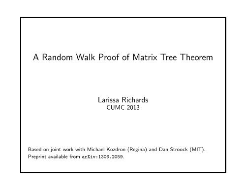
A <strong>Random</strong> <strong>Walk</strong> <strong>Pro<strong>of</strong></strong> <strong>of</strong> <strong>Matrix</strong> <strong>Tree</strong> <strong>Theorem</strong>Larissa RichardsCUMC 2013Based on joint work with Michael Kozdron (Regina) and Dan Stroock (MIT).Preprint available from arXiv:1306.2059.
Outline• Kirchh<strong>of</strong>f’s <strong>Matrix</strong> <strong>Tree</strong> <strong>Theorem</strong>• <strong>Random</strong> <strong>Walk</strong> on a Graph• Wilson’s Algorithm• <strong>Pro<strong>of</strong></strong> <strong>of</strong> Wilson’s Algorithm and Kirchh<strong>of</strong>f’s <strong>Matrix</strong> <strong>Tree</strong> <strong>Theorem</strong>• Application: Cayley’s Formula1
Set-upSuppose that Γ = (V,E) is a finite graph consisting <strong>of</strong> n+1 vertices labelledy 1 ,y 2 ,··· ,y n ,y n+1 .• undirected• connected• no multiple edgesNote that y i ∼ y j are nearest neighbours if (y i ,y j ) ∈ E.y 1 y 5y 4y 3 y 2y 62
The Graph Laplacian <strong>Matrix</strong>Recall that the graph Laplacian L is the matrix L = D −A, where D is the degreematrix and A is the adjacency matrix.y 1 y 5y 4y 3 y 2y 6L =y 1 y 2 y 3 y 4 y 5 y 6⎡y 1 3 0 −1 −1 −1 0y 2 0 2 0 −1 0 −1y 3 −1 0 3 −1 0 −1y 4 −1 −1 −1 4 −1 0⎢y 5 ⎣ −1 0 0 −1 2 0y 6 0 −1 −1 0 0 2⎤⎥⎦3
Kirchh<strong>of</strong>f’s <strong>Matrix</strong> <strong>Tree</strong> <strong>Theorem</strong>Suppose that L {k} denotes the submatrix <strong>of</strong> L obtained by deleting row k andcolumn k corresponding to vertex y k .Suppose that λ 1 ,λ 2 ,··· ,λ n are the nonzero eigenvalues <strong>of</strong> L.<strong>Theorem</strong> (Kirchh<strong>of</strong>f). If Ω = {spanning trees <strong>of</strong> Γ}, thendet[L {1} ] = det[L {2} ] = ··· = det[L {n} ] = det[L {n+1} ] = λ 1···λ nn+1and that these are equal to |Ω|, the number <strong>of</strong> spanning trees <strong>of</strong> Γ.Practically, this is very hard to compute!Usual modern way to prove MTT is purely algebraic and involves Cauchy-Binetformula.4
ExampleThis graph has 29 spanning trees.To see this, consider deg(y 4 ) in the spanning tree.y 1 y 5y 4y 3 y 2y 6deg(y 4 ) No. Spanning <strong>Tree</strong>s4 23 102 131 4295
Example (cont.)This graph has 29 spanning trees. For example, using MTT, det[L {5} ] = 29.y 1 y 5y 4y 3 y 2y 6L {5} =y 1 y 2 y 3 y 4 y 6⎡y 1 3 −1 −1 −1 0y 2 −1 2 −1 0 0y 3 −1 −1 4 −1 −1⎢y 4 ⎣ −1 0 −1 3 0y 6 0 0 −1 0 2⎤⎥⎦6
Example: <strong>Random</strong> <strong>Walk</strong> on a GraphChoose the next step equally likely from among all possible nearest neighbours.y 1 y 5y 4y 3 y 2y 6P = D −1 A =y 1 y 2 y 3 y 4 y 5 y 6⎡1y 1 0 03y 2 0 0 01y 3 0 03 1 1y 4 4 4⎢ 1y 5 ⎣ 0 02y 6 012140131021031301213140120 0120 0 0⎤⎥⎦7
<strong>Random</strong> <strong>Walk</strong> on a GraphFormally, a simple random walk {S k , k = 0,1,···} on graph Γ is a timehomogeneousMarkov Chain with transition probabilitiesP{S k+1 = y j | S 0 = y i0 ,··· ,S k−1 = y ik−1 ,S k = y i }= P{S k+1 = y j | S k = y i }= P{S 1 = y j | S 0 = y i }= p(i,j)where p(i,j) is the (i,j)-entry <strong>of</strong> P = D −1 A.Note thatp(i,j) =⎧⎨ 1deg(y i ) , if y i ∼ y j⎩0, else.8
<strong>Random</strong> <strong>Walk</strong> on a GraphRecall. The graph Laplacian matrix L is defined by L = D −A.We can rewrite it asL = D(I−D −1 A) = D(I−P).Let ∆ ⊂ V, ∆ ≠ ∅. ThenL ∆ = D ∆ (I ∆ −P ∆ )for the matrices obtained by deleting the rows and columns associated to theentries in ∆.Note that P ∆ is strictly substochastic; that is, non-negative entries and rows sumto at most 1 with at least one row sum less than 1.Thus (I ∆ −P ∆ ) −1 exists.9
The Key <strong>Random</strong> <strong>Walk</strong> FactsLet ζ ∆ = inf{j ≥ 0 : S j ∈ ∆} be the first time the random walk visits ∆ ⊂ V.For x,y /∈ ∆, let[ ∞]∑G ∆ (x,y) = E x 1{S k = y, k < ζ ∆ }k=0be the expected number <strong>of</strong> visits to y by simple random walk on Γ starting at xbefore entering ∆.This is <strong>of</strong>ten called the random walk Green’s function.• If G ∆ = [G ∆ (x,y)] x,y∈V \∆ , thenG ∆ = (I ∆ −P ∆ ) −1 .• If r ∆ (x) denotes the probability that simple random walk starting at x returnsto x before entering ∆, thenG ∆ (x,x) =∞∑r ∆ (x) k =k=011−r ∆ (x) .10
Wilson’s Algorithm (1996)Wilson’s Algorithm generates a spanning tree uniformly at random withoutknowing the number <strong>of</strong> spanning trees.• Pick any vertex. Call it v.• Relabel remaining vertices x 1 ,··· ,x n .• Start a simple random walk at x 1 . Stop it the first time it reaches v.• Erase loops.• Find the first vertex not in the backbone.• Start a simple random walk at it.• Stop it when it hits the backbone.• Erase loops.• Repeat until all vertices are included in the backbone.Clearly, this generates a spanning tree. We will prove that it is uniform among allpossible spanning trees.11
Example: Wilson’s Algorithm on ΓIt is easier to explain this example illustrating Wilson’s algorithm withoutrelabelling the vertices.Start a SRW at y 2 . Stop it when it first reaches y 1 .Assume the loop-erasure is [y 2 ,y 4 ,y 1 ]. Add this branch to the spanning tree.y 1 y 5y 1 y 5y 4y 4y 3 y 2y 6y 3 y 2y 612
Example: Wilson’s Algorithm on ΓStart a SRW at y 3 . Stop it when it reaches {y 2 ,y 4 ,y 1 }.Assume the loop-erasure is [y 3 ,y 6 ,y 2 ]. Add this branch to the spanning tree.y 1 y 5y 1 y 5y 4y 4y 3 y 2y 6y 3 y 2y 613
Example: Wilson’s Algorithm on ΓFinally, start a SRW at y 5 and stop it when it reaches {y 2 ,y 4 ,y 1 }∪{y 3 ,y 6 }.Assume the loop-erasure is [y 5 ,y 4 ]. Add this branch to the spanning tree.y 1 y 5y 1 y 5y 4y 4y 3 y 2y 6y 3 y 2y 6We have generated a spanning tree <strong>of</strong> Γ with three branches∆ 1 = [y 2 ,y 4 ,y 1 ], ∆ 2 = [y 3 ,y 6 ,y 2 ], ∆ 3 = [y 5 ,y 4 ].14
Some History• Kirchh<strong>of</strong>f - 1800sGustav Kirchh<strong>of</strong>f was motivated to study spanning trees by problems arisingfrom his work on electrical networks.• Wilson’s Algorithm - 1996David Wilson used “cycle-popping” to prove his algorithm generated a uniformspanning tree. His original pro<strong>of</strong> is <strong>of</strong> a very different flavour. The <strong>Matrix</strong> <strong>Tree</strong><strong>Theorem</strong> does not follow directly from the cycle-popping pro<strong>of</strong>.• Greg Lawler - 1999Lawler discovered a new, computational pro<strong>of</strong> <strong>of</strong> Wilson’s Algorithm viaGreen’s functions. The <strong>Matrix</strong> <strong>Tree</strong> <strong>Theorem</strong> follows immediately as a corollaryto his pro<strong>of</strong>.Our original goal was to give an expository account <strong>of</strong> Lawler’s pro<strong>of</strong>. However, inaddition to simplifying his pro<strong>of</strong>, we discovered that these ideas could be applied todeduce results for Markov processes.15
Suppose ∆ ⊂ V, ∆ ≠ ∅.Computing a Loop-Erased <strong>Walk</strong> ProbabilityLet x 1 ,··· ,x K be distinct elements <strong>of</strong> a connected subset <strong>of</strong> V\∆ labelled in sucha way that x j ∼ x j+1 for j = 1,··· ,K. Note that x K+1 ∈ ∆.Consider simple random walk on Γ starting at x 1 . Set ξ ∆ = inf{j ≥ 0 : S j ∈ ∆}.LetP ∆ (x 1 ,··· ,x K ,x K+1 ) := P{L({S j , j = 0,··· ,ξ ∆ }) = [x 1 ,··· ,x K ,x K+1 ]}denote the probability that loop-erasure <strong>of</strong> {S j , j = 0,··· ,ξ ∆ } is exactly[x 1 ,··· ,x K+1 ].16
Computing a Loop-Erased <strong>Walk</strong> ProbabilityQuestion: How can we computeP{L({S j , j = 0,··· ,ξ ∆ }) = [x 1 ,··· ,x K ,x K+1 ]}?For the loop-erasure to be exactly [x 1 ,··· ,x K+1 ], we need that:• the SRW started at x 1 , then• made a number <strong>of</strong> loops back to x 1 without entering ∆, then• took a step from x 1 to x 2 , then• made a number <strong>of</strong> loops back to x 2 without entering ∆∪{x 1 }, then• took a step from x 2 to x 3 , then• made a number <strong>of</strong> loops back to x 3 without entering ∆∪{x 1 ,x 2 }, then• ···• made a number <strong>of</strong> loops back to x K without entering∆∪{x 1 ,x 2 ,··· ,x K−1 }, then• took a step from x K to x K+1 ∈ ∆.17
Computing a Loop-Erased <strong>Walk</strong> ProbabilitySo,P ∆ (x 1 ,··· ,x K+1 )=∞∑m 1 ,···,m K =0r ∆ (x 1 ) m 1p(x 1 ,x 2 )r ∆∪{x1 }(x 2 ) m 2p(x 2 ,x 3 )······r ∆∪{x1 ,···,x K−1 }(x K ) m Kp(x K ,x K+1 )=K∏j=11deg(x j )11−r ∆(j) (x j )=K∏j=11deg(x j ) G ∆(j)(x j ,x j )where ∆(1) = ∆ and ∆(j) = ∆∪{x 1 ,··· ,x j−1 } for j = 2,··· ,K and the lastline follows from the key random walk fact.18
<strong>Pro<strong>of</strong></strong> <strong>of</strong> Wilson’s AlgorithmSuppose that T ∈ Ω was produced by Wilson’s algorithm with branches∆ 0 = {v}, ∆ 1 = [x 1,1 ,··· ,x 1,k1 ],··· ,∆ L = [x L,1 ,··· ,x L,kL ].We know that each branch in Wilson’s algorithm is generated by a loop-erasedrandom walk.P(T is generated by Wilson’s algorithm) =L∏P ∆l (x l,1 ,··· ,x l,kl )l=1where ∆ l = ∆ 0 ∪···∪∆ l−1 for l = 1,··· ,L.19
<strong>Pro<strong>of</strong></strong> <strong>of</strong> Wilson’s AlgorithmRecall: The Loop-Erased <strong>Walk</strong> Probability CalculationP ∆ (x 1 ,··· ,x K ,x K+1 ) =K∏j=1G ∆(j) (x j ,x j ).deg(x j )Hence, the probability that T is generated by Wilson’s algorithm isL∏P ∆l (x l,1 ,··· ,x l,kl ) =l=1L∏l=1k l −1∏j=1G ∆ l (j)(x l,j ,x l,j )deg(x l,j )where ∆ l (1) = ∆ l and ∆ l (j) = ∆ l ∪{x l,1 ,··· ,x l,j−1 } for j = 2,··· ,k l −1.To finish the pro<strong>of</strong> we need some facts from linear algebra.20
Some Linear AlgebraM is a non-degenerate N ×N matrix and ∆ ⊂ {1,2,··· ,N}.M ∆ : matrix formed by deleting rows and columns corresponding to indices in ∆.1. Cramer’s Rule(M −1 ) ii = det[M{i} ]det[M]2. Suppose (σ(1),··· ,σ(N)) is a permutation <strong>of</strong> (1,··· ,N). Set ∆ 1 = ∅ andfor j = 2,··· ,N, let ∆ j = ∆ j−1 ∪{σ(j −1)} = {σ(1),··· ,σ(j −1)}. IfM ∆(j) is non-degenerate for all j = 1,··· ,N, thendet[M] −1 =N∏(M ∆ j) −1j=1σ(j),σ(j) .21
<strong>Pro<strong>of</strong></strong> <strong>of</strong> Wilson’s AlgorithmRecall that we picked an arbitrary vertex v where we stopped our initial walk.Also recall that G ∆ = (I ∆ −P ∆ ) −1 and L ∆ = D ∆ (I ∆ −P ∆ ).By Linear Algebra fact 2,ThusL∏l=1k l −1∏j=1G ∆ l (j) (x l,j,x l,j ) = det[G {v} ].P(T is generated by Wilson’s algorithm) = det[G{v} ]det[D {v} ] = 1det[D {v} ]det[I {v} −P {v} ]= det[L {v} ] −1 .In addition, we can see that the right hand side <strong>of</strong> the equation is independent <strong>of</strong>the ordering <strong>of</strong> the remaining n vertices. Thus,P(T is generated by Wilson’s algorithm) = det[L {v} ] −1 = 1|Ω|22
Corollary: <strong>Pro<strong>of</strong></strong> <strong>of</strong> the <strong>Matrix</strong> <strong>Tree</strong> <strong>Theorem</strong>SinceP(T is generated by Wilson’s algorithm) = det[L {v} ] −1 = 1|Ω|we haveSince v was arbitrary, we conclude|Ω| = det[L {v} ].|Ω| = det[L {1} ] = det[L {2} ] = ··· = det[L {n} ] = det[L {n+1} ].Note. A separate argument is needed to show that|Ω| = λ 1···λ nn+1where λ 1 ,...,λ n are the non-zero eigenvalues <strong>of</strong> L. (This is found in our paper,but not in this talk.)23
Application: Cayley’s FormulaIf Γ = (V,E) is a complete graph on N +1 vertices; i.e., there is an edgeconnecting any two vertices in V. ThenNumber <strong>of</strong> spanning trees <strong>of</strong> Γ = (N +1) N−1 .15 243The number <strong>of</strong> spanning trees <strong>of</strong> K 5 is 5 3 = 125.24
Start a simple random walk at x.Application: Cayley’s FormulaSuppose that ∆ ⊂ V\{x}, where ∆ ≠ ∅, |∆| = m.Recall.r ∆ (x) is the probability that simple random walk starting at x returns to x beforeentering ∆.Let r ∆ (x;k) be the probability that simple random walk starting at x returns to xin exactly k steps without entering ∆ so thatr ∆ (x) =∞∑r ∆ (x;k).k=2Note that a SRW cannot return to its starting point in only 1 step.25
Application: Cayley’s FormulaSince Γ is the complete graph on N +1 vertices, we have partitioned the vertex set:V 1 = {x}, V 2 = ∆ with |V| = m, and V 3 with |V 3 | = N −m.Thus,and sor ∆ (x;k) = P{S 0 = x, S 1 ∈ V 3 ,··· ,S k−1 ∈ V 3 ,S k = x}= N −m ( ) N −1−m k−21N N Nr ∆ (x) = N −mN 2∞ ∑k=2= N −mN(m+1) .( N −1−mN) k−226
By the key random walk fact,Application: Cayley’s FormulaG ∆ (x,x) =11−r ∆ (x) = N(m+1)m(N +1) .(∗)Now, suppose that the vertices <strong>of</strong> Γ are {x 1 ,...,x N+1 }. Start the SRW at x 1 andassume that ∆ j = {x 1 ,...,x j } for j = 1,...,N.Since |∆ j | = j, we have from our linear algebra fact and (∗) thatdet[G {x 1} ] =N∏j=1G ∆j (x j ,x j ) =N∏j=1N(j +1)j(N +1) = NN (N +1)!(N +1) N N! = N N(N +1) N−1.Since each <strong>of</strong> the (N +1) vertices has degree N, we conclude|Ω| = det[D{x 1} ]det[G {x 1} ] =N N= (N +1) N−1 .N N(N+1) N−127
Thank you.28