Permanent Magnets - CERN Accelerator School
Permanent Magnets - CERN Accelerator School
Permanent Magnets - CERN Accelerator School

Create successful ePaper yourself
Turn your PDF publications into a flip-book with our unique Google optimized e-Paper software.
<strong>Permanent</strong> <strong>Magnets</strong><br />
Including Wigglers and Undulators<br />
Part II<br />
Johannes Bahrdt<br />
June 20th-22nd, 2009
Overview<br />
Part II<br />
Metallurgic aspects of permanent magnets<br />
Magnetic domains<br />
Observation techniques of magnetic domains<br />
New materials<br />
Aging / damage of permanent magnets<br />
Simulation methods<br />
PPM quadrupoles<br />
Johannes Bahrdt, HZB für Materialien und Energie, <strong>CERN</strong> <strong>Accelerator</strong> <strong>School</strong> „<strong>Magnets</strong>“, June 16th-25th, Bruges, Belgium, 2009
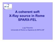
Crystal Structure of RE-<strong>Permanent</strong> <strong>Magnets</strong> I<br />
Unit cell of tetragonal<br />
Nd2Fe17B in reality the ratio c/a is smaller<br />
The Fe layers couple<br />
antiferromagnetically to the Nd, B layers<br />
Partial substitution of Nd with Dy<br />
crystal anisotropy increases<br />
coercivity increases<br />
Dy atoms couple antiparallel<br />
saturation magnetization<br />
decreases simultaneously<br />
J. Herbst, Review of Modern Physics,<br />
Vol. 63, No. 4 (1991) p819.<br />
Johannes Bahrdt, HZB für Materialien und Energie, <strong>CERN</strong> <strong>Accelerator</strong> <strong>School</strong> „<strong>Magnets</strong>“, June 16th-25th, Bruges, Belgium, 2009
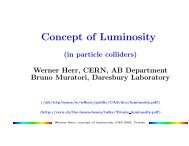
Crystal Structure of RE-<strong>Permanent</strong> <strong>Magnets</strong> II<br />
Unit cell of rhombohedral<br />
Co17 (R=Sm Tm=Co)<br />
Sm 2<br />
Unit cell of the hexagonal<br />
SmCo5 (R=Sm Tm=Co)<br />
J. Herbst, Review of Modern Physics,<br />
Vol. 63, No. 4 (1991) p819.<br />
Johannes Bahrdt, HZB für Materialien und Energie, <strong>CERN</strong> <strong>Accelerator</strong> <strong>School</strong> „<strong>Magnets</strong>“, June 16th-25th, Bruges, Belgium, 2009
Metallurgy: Theoretic Limits of Magnet properties<br />
Theoretical<br />
( BH ) =<br />
Typical<br />
ρ<br />
ρ<br />
0<br />
≥<br />
99%<br />
fϕ<br />
≥ 98%<br />
limit<br />
max Br<br />
2<br />
values<br />
due<br />
for<br />
sintered<br />
NdFeB<br />
to liquid phase<br />
alignmnet<br />
theoretic<br />
of energy<br />
/ μ<br />
product:<br />
B ( 20°<br />
C)<br />
= B<br />
⎛ Br<br />
ϕ = arctan⎜2<br />
⎜<br />
⎝ B<br />
coefficient<br />
= cos( ϕ)<br />
limit: 63 MGOe<br />
f<br />
magnets<br />
sintering<br />
Johannes Bahrdt, HZB für Materialien und Energie, <strong>CERN</strong> <strong>Accelerator</strong> <strong>School</strong> „<strong>Magnets</strong>“, June 16th-25th, Bruges, Belgium, 2009<br />
r<br />
ϕ<br />
for<br />
r−<br />
sat<br />
r−<br />
par<br />
isostatic<br />
ρ<br />
( 20°<br />
C)<br />
⋅ ⋅(<br />
1−V<br />
ρ<br />
− perp<br />
⎞<br />
⎟<br />
⎠<br />
pressing<br />
(achieved: 59 MGOe)<br />
0<br />
nonmagnetic<br />
< 2.5 wt.% of impurities like Nd-oxide<br />
requires vacuum induction furnace and inert gas processing<br />
< 2.5 wt.% of RE constituents<br />
< 0.<br />
05<br />
Vnonmagnetic<br />
) ⋅ f<br />
ϕ
Typical Structure of Sintered NdFeB<br />
The interesting effects<br />
happen at the boundaries!<br />
Nd2Fe14B grains<br />
<strong>Magnets</strong><br />
(monocrystalline)<br />
RE rich constituents containing<br />
Nd, Co, Cu, Al, Ga, Dy (area is exaggerated)<br />
Nd oxides<br />
Nd + H2O NdOH + H<br />
H + Nd NdH<br />
appropriate chemical<br />
additions between grains<br />
avoid Hydrogen decrepitation<br />
Hydrogen decrepitation destroys magnetic material<br />
- fatal for magnets in operation<br />
- ecologically interesting for decomposition and RE recovery<br />
Johannes Bahrdt, HZB für Materialien und Energie, <strong>CERN</strong> <strong>Accelerator</strong> <strong>School</strong> „<strong>Magnets</strong>“, June 16th-25th, Bruges, Belgium, 2009
Coercivity<br />
In the bulk magnetic domains are separated by Bloch walls:<br />
below a certain size: no Bloch walls can exist due to energetic considerations<br />
above that size several domains in one particle are possible<br />
critical size for Fe: 0.01 μm, for Ba ferrite: 1 μm<br />
above that size remanence and coercivity follow roughly a 1/size dependence<br />
RE-magnets have typical grain sizes that are a bit larger than single domain size<br />
normally, the rotation of the magnetization vector occurs in the boundary plane<br />
In thin films: Neel walls, magnetization vector rotates perpendicular to boundary<br />
Reason for coercivity:<br />
- intentionally introduced imperfections (e.g. carbides in steel magnets)<br />
impede the movement of Bloch walls<br />
- stable single domain grains which can be switched only completely<br />
- introduction of anisotropy<br />
Basically two types of anisotropy:<br />
- shape of microscopic magnetic parts in non magnetic matrix (needles etc)<br />
- crystal anisotropy<br />
Johannes Bahrdt, HZB für Materialien und Energie, <strong>CERN</strong> <strong>Accelerator</strong> <strong>School</strong> „<strong>Magnets</strong>“, June 16th-25th, Bruges, Belgium, 2009
Two Classes of <strong>Magnets</strong><br />
A) Small particle magnets with shape anisotropy<br />
shaped magnetic material in non magnetic matrix<br />
e.g. FeCo in less magnetic FeNiAl (AlNiCo) or nonmagnetic lead matrix<br />
Shape anisotropy of AlNiCo 5:<br />
Spinodal decompostion<br />
energy product largest along<br />
direction of needles (factor of 10 as<br />
compared to perpendicular direction)<br />
B) Small particle magnets with crystalline anisotropy<br />
- Nucleation type, e.g. SmCo5 , Nd2 Fe14 B, ferrites<br />
easy motion of domain walls within one domain;<br />
motion impeded at grain walls<br />
FeCo<br />
FeNiAl-matrix<br />
- Pinning type, e.g. Sm(Co, Fe, Cu, Hf) 7 , SmCo 5 + Cu precipitation,<br />
Sm 2 Co 17 with SmCo 5 precipitation (size of domain wall thickness)<br />
Domain walls are pinned to boundaries of precipitations<br />
Johannes Bahrdt, HZB für Materialien und Energie, <strong>CERN</strong> <strong>Accelerator</strong> <strong>School</strong> „<strong>Magnets</strong>“, June 16th-25th, Bruges, Belgium, 2009
Initial Magnetization<br />
M<br />
initial magnetization<br />
Nucleation type magnet<br />
directly after heating: many domain walls inside each grain<br />
Bloch walls are rather freely movable within grains<br />
high initial permeability; walls are pushed out of grain bulk at first magentization<br />
fixing of walls at the grain boundaries<br />
usually no domain walls within grain bulk under fully magnetized conditions<br />
in reverse field most grains switch completely the magentization<br />
Pinning type magnet<br />
pinning centers inside grains impede wall movement<br />
high fields are required to move the walls<br />
Johannes Bahrdt, HZB für Materialien und Energie, <strong>CERN</strong> <strong>Accelerator</strong> <strong>School</strong> „<strong>Magnets</strong>“, June 16th-25th, Bruges, Belgium, 2009<br />
H
Metallurgy I: Coercivity<br />
Versus Grain Size<br />
Partial replacement of Nd with Dy enhances the anisotropy field<br />
and thus the coercivity, however:<br />
Dy is expensive & remanence is reduced<br />
Use all means to enhance coercivity without Dy, e.g. optimizing the grain size<br />
Systematic studies show:<br />
Within the grain size range of 3.9 and 7.6 μm<br />
the coercivity increases with smaller grain size<br />
H cj<br />
Powder size<br />
μm<br />
H cj<br />
Grain size<br />
μm<br />
−0.<br />
44<br />
( )<br />
( 20°<br />
C)<br />
∝ grainsize<br />
Hcj<br />
(20°C)<br />
kA/m<br />
1,9 3,8 1178 581<br />
2,2 4,3 1162 573<br />
2,6 4,9 1090 525<br />
3,0 6,0 971 462<br />
3,5 7,6 883 414<br />
Hcj (100°C)<br />
kA/m<br />
K. Uestuener, M. Katter,<br />
W Rodewald, 2006<br />
Johannes Bahrdt, HZB für Materialien und Energie, <strong>CERN</strong> <strong>Accelerator</strong> <strong>School</strong> „<strong>Magnets</strong>“, June 16th-25th, Bruges, Belgium, 2009
Metallurgy II: Remanence and Coercivity<br />
Versus Alignment Angle and External Field Direction<br />
with inreasing alignment coefficient:<br />
- remanence increases<br />
- coercivity decreases<br />
dependence<br />
rough<br />
W. Rodewald et al., VAC, Hagener<br />
Symposium für Pulvermetallurgie,<br />
Band 18 (2002) pp 225 -245.<br />
of coercivity<br />
approximation:<br />
on applied<br />
H cj<br />
∝<br />
1<br />
cos( θ )<br />
external<br />
field<br />
direction:<br />
detailed study at 0°, 45° 90° shows:<br />
- nearly no difference between 0° and 45°<br />
- increase of Hcj by - 30% for axially pressed material<br />
- 70% for isostatically pressed material<br />
in specific cases this enhancement of coercivity can be used.<br />
M. Katter Transactions on <strong>Magnets</strong>, Vol: 41, No:10, (2005)<br />
Johannes Bahrdt, HZB für Materialien und Energie, <strong>CERN</strong> <strong>Accelerator</strong> <strong>School</strong> „<strong>Magnets</strong>“, June 16th-25th, Bruges, Belgium, 2009
Metallurgy III: Permeability Versus Coercivity<br />
Linear superposition of PPM fields works within a few percent.<br />
For higher accuracy non unity of permeability has to be regarded.<br />
μ par<br />
μ perp<br />
depends on fabrication process<br />
1.05 axially pressed<br />
1.03 isostatically pressed<br />
no correlation with coercivity<br />
decreases with increasing coercivity<br />
1.17 (Hcj=18kOe), 1.12 (Hcj=32kOe) M. Katter Transactions on <strong>Magnets</strong>, Vol: 41, No:10, (2005)<br />
Johannes Bahrdt, HZB für Materialien und Energie, <strong>CERN</strong> <strong>Accelerator</strong> <strong>School</strong> „<strong>Magnets</strong>“, June 16th-25th, Bruges, Belgium, 2009
Metallurgy IV: Grain Growth During Sintering<br />
Study of grain size growth with ASTM E112<br />
(ASTM E112 is a standard for grain size measurement)<br />
the grain radius inceases over time approximately with<br />
R(<br />
t)<br />
= k ⋅t<br />
1/<br />
n<br />
n = 2-4 for pure metals<br />
n = 16-20 for sintered NdFeB with B < 5.7at.%<br />
n = 7.5 for sintered NdFeB magnets with B > 5.7 at.%<br />
n = 10 for sintered NdFeB magnets with RE-contituents > 4wt.%<br />
sintering time has to be adjusted appropriately<br />
to achieve an optimum grain size of 3-5μm and to avoid giant grains<br />
NdFeB has hexagonal structure<br />
Distribution of numbers of corners changes during sintering<br />
optimization of six corner grains<br />
Grains in a sintered NdFeB magnet,<br />
averaged grain size: 4.6μm;<br />
polished and chemical etched surface as<br />
seen with a conventional light microscope<br />
Johannes Bahrdt, HZB für Materialien und Energie, <strong>CERN</strong> <strong>Accelerator</strong> <strong>School</strong> „<strong>Magnets</strong>“, June 16th-25th, Bruges, Belgium, 2009<br />
Courtesy of VAC
Methods of Magnetic Domain Measurement I<br />
Bitter Patterns<br />
Ferrofluids: fine magnetic grains (a few tens of nm) in a colloid<br />
suspension is spread on a polished surface of a magnetic sample<br />
magnetic grains are attracted at the domain walls<br />
Resolution: 100nm<br />
Magnetooptical effects:<br />
- Kerr-effect (MOKE), reflection geometry<br />
- Faraday-effect, transmission geometry<br />
Resolution: 150nm, suitable for the detection of fast processes<br />
All magnetooptical effects can be described with a generalized<br />
dielectric permittvity tensor which reduces for cubic crystals to:<br />
2<br />
⎛ 1 − iQ<br />
⎛<br />
⎞<br />
V m3<br />
iQvm2<br />
⎞ B1m1<br />
B2m1m<br />
2 B2m1m<br />
3<br />
⎜<br />
⎟ ⎜<br />
⎟<br />
2<br />
ε = ε⎜<br />
iQvm3<br />
1 − iQvm1<br />
⎟ + ⎜ B2m1m<br />
2 B1m2<br />
B2m2m3<br />
⎟<br />
⎜<br />
⎟ ⎜<br />
2 ⎟<br />
⎝−<br />
iQvm2<br />
iQvm1<br />
1 ⎠ ⎝ B2m1m<br />
3 B2m2m3<br />
B1m3<br />
⎠<br />
Similarly, a magnetic permeability tensor can be set up, however,<br />
the coefficients are 2 orders of magnitude smaller and usually neglected<br />
Inserting these tensors into Fresnel’s equation describes all effects<br />
r<br />
Johannes Bahrdt, HZB für Materialien und Energie, <strong>CERN</strong> <strong>Accelerator</strong> <strong>School</strong> „<strong>Magnets</strong>“, June 16th-25th, Bruges, Belgium, 2009
Methods of Magnetic Domain Measurement II<br />
Geometries<br />
polar magnetization<br />
parallel to plane of inc.<br />
rotation of reflected<br />
and transmitted light<br />
clockwise<br />
of magnetooptical<br />
longitudinal magn.<br />
parallel<br />
rotation of reflected<br />
and transmitted light<br />
counter clockwise<br />
Kerr-<br />
- linearly polarized light forces charges to vibrational motion<br />
- moving charges experience Lorentz forces<br />
- the additional vibrational motion introduces perpendicaular<br />
electric field component in reflected / transmitted beam<br />
and Farady-effect<br />
longitudinal magn.<br />
perpendicular<br />
Kerr: clockwise<br />
Faraday:<br />
counter clockwise<br />
http://upload.wikimedia.org/wikipedia/commons/b/b4/NdFeB-Domains.jpg<br />
transverse magn.<br />
parallel<br />
Kerr: same direction<br />
change of amplitude<br />
Farady: no effect in transm.<br />
Johannes Bahrdt, HZB für Materialien und Energie, <strong>CERN</strong> <strong>Accelerator</strong> <strong>School</strong> „<strong>Magnets</strong>“, June 16th-25th, Bruges, Belgium, 2009
Methods of Magnetic Domain Measurement III<br />
X-Ray Magnetic Circular Dichroism (XMCD)<br />
Different absorption coeffficients of right / left handed circularly polarized light<br />
Photoelectron<br />
emission<br />
microscope<br />
W.Kuch et al., Phys. Rev. B,<br />
Vol 65, 0064406-1-7 (2002)<br />
(PEEM) at BESSY UE56 APPLE<br />
Exchange coupling between magnetic films of Co and Ni separated<br />
by a nonmagnetic layer of Cu with variable thickness<br />
Johannes Bahrdt, HZB für Materialien und Energie, <strong>CERN</strong> <strong>Accelerator</strong> <strong>School</strong> „<strong>Magnets</strong>“, June 16th-25th, Bruges, Belgium, 2009
Methods of Magnetic Domain Measurement IV<br />
X-Ray Holography<br />
No lenses or zone plates are needed<br />
resolution 50nm demonstrated so far<br />
Principle:<br />
absorption of coherent cicularly polarized light within an aperture of 1.5μm<br />
reference hole 100-350nm (conical)<br />
coherent overlap of both beams<br />
circularly polarizing<br />
undulator<br />
coherence<br />
pinhole<br />
sample &<br />
reference pinhole<br />
CCD camera<br />
measuring hologram<br />
S. Eisebitt et al, Phys. Rev. B 68, 104419-1-6 (2003)<br />
S. Eisebitt at al, Nature Vol. 432 (2004) pp 885-888<br />
Johannes Bahrdt, HZB für Materialien und Energie, <strong>CERN</strong> <strong>Accelerator</strong> <strong>School</strong> „<strong>Magnets</strong>“, June 16th-25th, Bruges, Belgium, 2009
Methods of Magnetic Domain Measurement V<br />
Neutron decoherence imaging<br />
advantage: thick samples (cm range) can be studied<br />
disadvantage: resolution so far 50-100 μm<br />
Principle:<br />
coherent neutrons from source grating (de Broglie waves)<br />
diffraction of neutrons at magnetic domain walls, distortion of wavefront<br />
Talbot image of distorted wavefront using phase grating<br />
detection of talbot image with sliding absorption grating and detector<br />
neutron<br />
source<br />
source grating<br />
object<br />
phase<br />
a few meters a few cm<br />
neutron<br />
detector<br />
grating sliding<br />
detection grating<br />
F. Pfeiffer et al., Phys. Rev. Let. 96. 215505-1-4, 2006<br />
C. Grünzweig et al., Phys. Rev. Let. 101, 025504, 2008<br />
Johannes Bahrdt, HZB für Materialien und Energie, <strong>CERN</strong> <strong>Accelerator</strong> <strong>School</strong> „<strong>Magnets</strong>“, June 16th-25th, Bruges, Belgium, 2009
Methods of Magnetic Domain Measurement VI<br />
Transmission electron microscope<br />
Lorentz force microscopy, resolution 10nm<br />
few 100MeV<br />
electrons<br />
Further methods<br />
XMCD in absorption or transmission geometry<br />
Low energy electron diffraction (LEED)<br />
Magnetic force microscope (resolution 10nm)<br />
Spin polarized scanning tunneling microscope (resolution 1nm)<br />
For other domain geometries<br />
tilting of the sample may be<br />
necessary for a net deflection<br />
few 100 nm thick<br />
ferromagnetic layer<br />
See also: A. Hubert, R. Schäfer, „Magnetic Domains“,<br />
Springer-Verlag, Berlin, Heidelberg, New York, 2000<br />
Johannes Bahrdt, HZB für Materialien und Energie, <strong>CERN</strong> <strong>Accelerator</strong> <strong>School</strong> „<strong>Magnets</strong>“, June 16th-25th, Bruges, Belgium, 2009
Cryogenic<br />
Cryogenic<br />
<strong>Permanent</strong> Magnet Undulators<br />
Proposed<br />
by<br />
T. Hara, T. Tanaka, H. Kitamura<br />
T. Hara et al. Phys. Rev. Spec. Topics, Vol. 7, 050702 (2004) 1-6<br />
T. Tanaka et al. Phys. Rev. Spec. Topics, Vol. 7, 090704 (2004) 1-5<br />
undulator for<br />
table<br />
top-FEL application<br />
et al.<br />
gain in magnetic field<br />
as compared to conventional<br />
in-vacuum undulator: 1.5<br />
mature technology<br />
gain of superconducting ID<br />
as compared to conventional<br />
in-vacuum undulator: 2.0<br />
many open questions<br />
New materials:<br />
- No spin reorientation<br />
for PrFeB magnets<br />
- Dy can be used as pole material<br />
below the phase transition at 80K<br />
saturation magnetization >3Tesla<br />
- Dy diffused magnets (Hitachi)<br />
Johannes Bahrdt, HZB für Materialien und Energie, <strong>CERN</strong> <strong>Accelerator</strong> <strong>School</strong> „<strong>Magnets</strong>“, June 16th-25th, Bruges, Belgium, 2009
Magnet Stablity, Magnet Aging I<br />
7000<br />
6900<br />
6800<br />
6700<br />
6600<br />
6500<br />
6400<br />
6300<br />
6200<br />
6100<br />
6000<br />
History of sector 3<br />
downstream undulator at APS<br />
5900<br />
0 20 40 60 80 100 120 140 160 180<br />
y<br />
Pole Number<br />
x<br />
1997<br />
2001<br />
2003<br />
2004<br />
Johannes Bahrdt, HZB für Materialien und Energie, <strong>CERN</strong> <strong>Accelerator</strong> <strong>School</strong> „<strong>Magnets</strong>“, June 16th-25th, Bruges, Belgium, 2009<br />
1.20E-01<br />
1.00E-01<br />
8.00E-02<br />
6.00E-02<br />
4.00E-02<br />
2.00E-02<br />
0.00E+00<br />
Hall probe scans have<br />
been performed at the<br />
dismounted magnets<br />
along the indicated paths<br />
x-scan<br />
Original<br />
Damaged<br />
-80 -60 -40 -20 0 20 40<br />
x [mm]<br />
0.10<br />
0.05<br />
0.00<br />
-0.05<br />
-0.10<br />
Original<br />
Damaged<br />
y-scan<br />
-0.15<br />
-80 -40 0 40 80<br />
y [mm]<br />
the damages are located close to the e-beam<br />
Field retuning has been done with<br />
- undulator tapering<br />
- magnet flipping or<br />
- remagnetizing of magnet blocks<br />
courtesy of L. Moog, APS, Argonne National Lab., operated by<br />
UChicago Argonne for US-DOE, contract DE-AC02-06CH11357<br />
5500<br />
5400<br />
5300<br />
5200<br />
5100<br />
5000<br />
4900<br />
4800<br />
4700<br />
4600<br />
before<br />
after<br />
Block flipping<br />
APS27#2<br />
4500<br />
0 20 40 60 80 100 120 140<br />
Pole #
Magnet Stablity, Magnet Aging II<br />
Demagnetization has been observed also at other out of vacuum devices:<br />
ESRF<br />
P. Colomp et al., Machine Technical Note 1-1996/ID, 1996<br />
DESY / PETRA H. Delsim-Hashemi<br />
In-vacuum applications are even more critical<br />
usage of SmCo or special grades of NdFeB<br />
et al., PAC Proceedings, Vancouver BC, Canada 2009<br />
is required<br />
Protection of magnets:<br />
- Collimator system<br />
- dogleg for energy filtering (used in linear accelerators)<br />
- apertures for off axis particles (LINACS and SR, e.g. SLS-SR)<br />
- Beam loss detection<br />
fast detection<br />
- scintillators: high sensitivity, medium spatial resolution<br />
- Cherenkov fibers: medium sensitivity, high spatial resolution<br />
absolute dose measurements<br />
- OTDR systems: simple but low dynamic<br />
- power meter fibers: using several coils: high dynamic<br />
Johannes Bahrdt, HZB für Materialien und Energie, <strong>CERN</strong> <strong>Accelerator</strong> <strong>School</strong> „<strong>Magnets</strong>“, June 16th-25th, Bruges, Belgium, 2009
Induced Loss [dB/km]<br />
10 5<br />
10 4<br />
10 3<br />
10 2<br />
10 1<br />
10 0<br />
10 -2<br />
Magnet Stablity, Magnet Aging III<br />
���������<br />
λ� ��������<br />
�� �� ����<br />
�� ������<br />
�� ������� �<br />
10 -1<br />
Powermeter fibers<br />
10 0<br />
calibration<br />
10 1<br />
����� ������� � ��<br />
10 2<br />
�����⋅�±���<br />
�����������<br />
������������<br />
������������<br />
�������������<br />
10 3<br />
10 4<br />
Dose [Gy]<br />
35<br />
30<br />
25<br />
20<br />
15<br />
10<br />
5<br />
0<br />
Channel 1<br />
Channel 2<br />
Channel 3<br />
Channel 4<br />
Channel 5<br />
Channel 6<br />
Channel 7<br />
Channel 8<br />
Channel 9<br />
Channel 10<br />
Channel 11<br />
Channel 12<br />
Channel 13<br />
Channel 14<br />
Channel 15<br />
Channel 16<br />
measured<br />
losses<br />
080411 1100 080411 1200 080411 1300 080411 1400 080411 1500 080411 1600<br />
Powermeter fibers as installed at the<br />
MAXlab-HZB HGHG-FEL<br />
Date<br />
Fibre<br />
position<br />
Cherenkov<br />
fibers<br />
0° losses 45° losses 90°<br />
losses<br />
45° 0.00255 0.00341 0.00277<br />
135° 0.00171 0.00186 0.00286<br />
225° 0.00194 0.00189 0.00193<br />
315° 0.00285 0.00206 0.00191<br />
Number of Cherenkov photons per electron<br />
J. Bahrdt et al, Proc. of FEL Conf.<br />
Novosibirsk Siberia (2007) pp122-225.<br />
J. Bahrdt et al, Proc of FEL Conference (2008)<br />
Johannes Bahrdt, HZB für Materialien und Energie, <strong>CERN</strong> <strong>Accelerator</strong> <strong>School</strong> „<strong>Magnets</strong>“, June 16th-25th, Bruges, Belgium, 2009
Equivalent Descriptions of <strong>Permanent</strong> <strong>Magnets</strong><br />
+ ++ + + + +<br />
- - - - - - -<br />
surface charge density<br />
at the pole faces<br />
r<br />
r ∇'⋅M<br />
( r')<br />
Φ( r0<br />
) = −∫<br />
r r dV '=<br />
r0<br />
− r ' ∫∫<br />
r r<br />
r<br />
H ( r ) = −grad(<br />
Φ(<br />
r ))<br />
0<br />
Assuming<br />
rectangular<br />
0<br />
surface<br />
magnets<br />
r r r<br />
n'⋅M<br />
( r ')<br />
dS'<br />
r r<br />
r − r '<br />
0<br />
with<br />
μpar=1, μperp=0 surface currents<br />
flowing at the sides<br />
of the magnet<br />
Johannes Bahrdt, HZB für Materialien und Energie, <strong>CERN</strong> <strong>Accelerator</strong> <strong>School</strong> „<strong>Magnets</strong>“, June 16th-25th, Bruges, Belgium, 2009<br />
x<br />
x<br />
xx<br />
x x<br />
x<br />
r r 1<br />
B(<br />
r0<br />
) =<br />
c<br />
r r<br />
B(<br />
r ) =<br />
0<br />
∫<br />
∫<br />
r<br />
Idl<br />
×<br />
This approach is called CSEM which means either<br />
- Current Sheet Equivalent Method or<br />
- Charge Sheet Equivalent Method<br />
r r<br />
r0<br />
− r '<br />
r r 3<br />
r0<br />
− r '<br />
r r<br />
r r0<br />
− r '<br />
( ∇×<br />
M ) × dV '<br />
r<br />
0<br />
r<br />
− r '<br />
3
Based on these equations the fields can be evaluated by<br />
analytic integrations over all current carrying surfaces<br />
contribution<br />
B<br />
B<br />
B<br />
x<br />
y<br />
z<br />
CSEM for a Rectangular Block<br />
=<br />
I<br />
c<br />
= 0<br />
⋅<br />
I<br />
= −<br />
c<br />
totally:<br />
from<br />
surface<br />
A:<br />
0<br />
∫∫<br />
2<br />
2<br />
2<br />
( x − x ) + ( y − y ) + ( z − z ) )<br />
r r r r<br />
B(<br />
r ) = Q(<br />
r ) ⋅ M<br />
Q<br />
Q<br />
x<br />
xx<br />
xy<br />
1,<br />
2<br />
0<br />
=<br />
2<br />
ijk = 1<br />
⋅<br />
⎛<br />
= ln⎜<br />
⎜<br />
⎝<br />
( y , z<br />
1,<br />
2<br />
0<br />
0<br />
∫∫<br />
2<br />
2<br />
2<br />
( x − x ) + ( y − y ) + ( z − z ) )<br />
2<br />
0<br />
∑ ( −1)<br />
∏<br />
ijk =<br />
1,<br />
2<br />
0<br />
i+<br />
j+<br />
k + 1<br />
y − y<br />
0<br />
⎛<br />
arctan<br />
⎜<br />
⎜<br />
⎝<br />
x<br />
x − x<br />
(<br />
2 2 2<br />
( zk<br />
+ xi<br />
+ y j + zk<br />
)<br />
i+<br />
j+<br />
k<br />
−1)<br />
⎞<br />
⎟<br />
1<br />
⎠<br />
) = x ( y , z ) − x ( y , z ) ± w<br />
c<br />
c<br />
c<br />
i<br />
0<br />
0<br />
x<br />
0<br />
2<br />
i<br />
y<br />
j<br />
0<br />
z<br />
k<br />
+ y<br />
2<br />
j<br />
0<br />
0<br />
+ z<br />
3/<br />
2<br />
2<br />
k<br />
dz ⋅dy<br />
3/<br />
2<br />
⎞<br />
⎟<br />
⎟<br />
⎠<br />
x(<br />
y,<br />
z)<br />
dz ⋅dy<br />
/ 2<br />
(xc,yc,zc (x0,y0,z0 (wx,wy,wz ) = center of magnet<br />
) = point of observation<br />
) = dimensions of magnet<br />
similarly for all Qij Johannes Bahrdt, HZB für Materialien und Energie, <strong>CERN</strong> <strong>Accelerator</strong> <strong>School</strong> „<strong>Magnets</strong>“, June 16th-25th, Bruges, Belgium, 2009<br />
z<br />
y<br />
A<br />
x<br />
B( x0,<br />
y0,<br />
z0)<br />
r
Arbitrary Magnetized Volumes<br />
Enclosed by Planar Polygones<br />
Similarly, the fields and field integrals from arbitrary current<br />
carrying planar polygons can be evaluated<br />
r r r r<br />
Field B(<br />
r0<br />
) = Q(<br />
r0<br />
) ⋅ M<br />
r r r<br />
r ( r0<br />
− r ')<br />
⊗ n'surface<br />
r<br />
Q(<br />
r0<br />
) = ∫∫ r r dr<br />
'<br />
3<br />
r − r '<br />
r r<br />
I ( r , v)<br />
=<br />
0<br />
r r<br />
G(<br />
r , v)<br />
=<br />
0<br />
surface<br />
∞<br />
∫<br />
−∞<br />
r r<br />
H ( r<br />
1<br />
2π<br />
0<br />
∫∫<br />
surface<br />
0<br />
r r r r<br />
+ v)<br />
dl = G(<br />
r , v)<br />
⋅ M<br />
r<br />
[ ( r '−r0<br />
) × v]<br />
× v]<br />
r r<br />
( r '−r<br />
) ×<br />
Q and G are 3x3 matrices describing<br />
the geometric shape of the magnetized cell<br />
They can be evaluated analytically for an<br />
arbitrary polyhedron<br />
denotes a dyadic product<br />
⊗<br />
Field integral<br />
r<br />
⊗ n'<br />
r 2<br />
v<br />
O. Chubar, P. Elleaume, J. Chavanne,<br />
J. of Synchrotron Radiation, 5 (1998) 481-484<br />
P. Elleaume, O. Chubar, J. Chavanne,<br />
Proc. of PAC Vancouver, BC, Canada,<br />
(1997) 3509-3511<br />
Johannes Bahrdt, HZB für Materialien und Energie, <strong>CERN</strong> <strong>Accelerator</strong> <strong>School</strong> „<strong>Magnets</strong>“, June 16th-25th, Bruges, Belgium, 2009<br />
r<br />
0<br />
r<br />
0<br />
surface r<br />
dr<br />
'
Finite Susceptibility Requires Iterative Algorithm<br />
For real magnets: μpar=1.06, μperp=1.17 Iterative algorithms are required to evaluate the fields.<br />
For pure permanet magnet structures<br />
the finite susceptibility lowers the<br />
evaluated undulator fields by a few percent<br />
as compared to zero susceptibility<br />
r<br />
B<br />
i<br />
H<br />
r<br />
M<br />
M<br />
i<br />
N<br />
= ∑Q<br />
k = 1<br />
k ≠i<br />
= B<br />
r<br />
i−<br />
par<br />
i−<br />
perp<br />
i<br />
k , i<br />
r<br />
⋅ M<br />
1<br />
= B<br />
4π<br />
= ( μ<br />
r<br />
perp<br />
k<br />
− 4π<br />
⋅ M<br />
r<br />
i<br />
+ Q<br />
+ ( μ<br />
ii<br />
par<br />
−1)<br />
⋅ H<br />
r<br />
⋅ M<br />
i<br />
−1)<br />
⋅ H<br />
i−<br />
perp<br />
i−<br />
par<br />
calculation<br />
start with<br />
magnetizations<br />
Johannes Bahrdt, HZB für Materialien und Energie, <strong>CERN</strong> <strong>Accelerator</strong> <strong>School</strong> „<strong>Magnets</strong>“, June 16th-25th, Bruges, Belgium, 2009<br />
get<br />
get<br />
get<br />
next<br />
internal<br />
internal<br />
new<br />
magnetic<br />
field<br />
strengths<br />
magentizations<br />
iteration<br />
of geometry<br />
factors<br />
M i<br />
for<br />
inductions<br />
H i<br />
Q ki<br />
(Hi=0) B i
Simulations in the Nonlinear Regime<br />
Linear regime<br />
M<br />
M<br />
par<br />
perp<br />
( H<br />
( H<br />
par<br />
perp<br />
Including<br />
M<br />
H<br />
χ<br />
r<br />
cj<br />
( T ) = M<br />
perp<br />
( T ) = H<br />
( T ) = χ<br />
) = M<br />
r<br />
) = χ<br />
+ χ<br />
perp<br />
H<br />
par<br />
H<br />
perp<br />
temperature<br />
r<br />
cj<br />
par<br />
dependence<br />
( T ) ⋅(<br />
1+<br />
a ( T −T<br />
) + a ( T −T<br />
)<br />
0<br />
( T ) ⋅(<br />
1+<br />
b ( T −T<br />
) + b ( T −T<br />
)<br />
perp<br />
0<br />
( T ) ⋅(<br />
1+<br />
a ( T −T<br />
) + a ( T −T<br />
)<br />
0<br />
1<br />
1<br />
Magnetization Ansatz<br />
3 ⎛ χi<br />
M ( H,<br />
T ) = α(<br />
T ) ∑ M tanh<br />
⎜ si ( H + H<br />
i=<br />
1 ⎝ M si<br />
1<br />
0<br />
0<br />
+ ...)<br />
+ ...)<br />
+ ...)<br />
ai, bi from data sheet of magnet supplier<br />
Msi, χi from fit of M(H) curve at T0 (magnet supplier)<br />
α(T) is determined from<br />
M r<br />
( H = 0,<br />
T ) = M ( T)<br />
0<br />
2<br />
2<br />
J. Chavanne et al., Proc. of EPAC,<br />
Vienna, Austria (2000) 2316-2318<br />
Johannes Bahrdt, HZB für Materialien und Energie, <strong>CERN</strong> <strong>Accelerator</strong> <strong>School</strong> „<strong>Magnets</strong>“, June 16th-25th, Bruges, Belgium, 2009<br />
2<br />
0<br />
0<br />
2<br />
2<br />
0<br />
2<br />
cj<br />
⎞<br />
( T ))<br />
⎟<br />
⎠<br />
Hcj(T0) Hcj(T) M<br />
Mr(T0) Mr(T) H<br />
This model has been<br />
implemented into RADIA<br />
and tested with a real<br />
magnet assembly
2-dimensional Geometries<br />
Use complex notation of fields:<br />
r<br />
* r<br />
B ( z0)<br />
= Bx<br />
− iBy<br />
r<br />
iϕ0<br />
z = x + iy = r ⋅e<br />
0<br />
B r<br />
0<br />
0<br />
* is an analytic function, is not<br />
Cauchy Riemann relations are<br />
equivalent to Maxwell equations.<br />
Examples:<br />
Current flowing into the plane:<br />
r<br />
* r jz<br />
B ( z0<br />
) = a∫<br />
r r ⋅dx<br />
⋅ dy<br />
z − z<br />
<strong>Permanent</strong> magnet with remanence<br />
r<br />
r<br />
* r Br<br />
B ( z0)<br />
= b∫<br />
r r ⋅dx<br />
⋅dy<br />
2<br />
( z0<br />
− z)<br />
B = B + iB<br />
r<br />
rx<br />
ry<br />
Optimization<br />
0<br />
0<br />
using<br />
B r<br />
conformal<br />
mapping<br />
Easy axis rotation theorem:<br />
rotation of all magnetization vectors by (+α)<br />
rotates the field vector B by (α) (Halbach)<br />
field<br />
at the<br />
B(x0,y0) center?<br />
Johannes Bahrdt, HZB für Materialien und Energie, <strong>CERN</strong> <strong>Accelerator</strong> <strong>School</strong> „<strong>Magnets</strong>“, June 16th-25th, Bruges, Belgium, 2009<br />
B r<br />
r
Multipole<br />
n ⎛<br />
⎜ ⎛ r<br />
1−<br />
n 1⎜<br />
⎜<br />
− r<br />
⎝ ⎝<br />
<strong>Magnets</strong> for <strong>Accelerator</strong>s I<br />
Halbach type multipoles<br />
General segmented multipole with stacking factor ε≤1<br />
ν=harmonic number (v=0 describes the fundamental)<br />
N=order of multipole, N=1: dipole, N=2: quadrupole etc<br />
Br=remanence r1=inner radius<br />
r2=outer radius<br />
M=total number of magnets per period<br />
α = (N+1)2π/M = relative angle of magnetization between segments<br />
n−1<br />
r<br />
∞ r<br />
* r r ⎛ z ⎞ n ⎛ r<br />
B ( z)<br />
B<br />
⎜ ⎛<br />
= r∑<br />
⎜ 1<br />
0 r ⎟ −<br />
1 n 1⎜<br />
⎜<br />
ν = ⎝ ⎠ − r<br />
⎝ ⎝<br />
n sin( nεπ<br />
/ M )<br />
Kn<br />
= cos ( επ / M )<br />
nπ<br />
/ M<br />
n = N + νM<br />
1<br />
2<br />
⎞<br />
⎟<br />
⎠<br />
n−1<br />
⎞<br />
⎟<br />
⎟<br />
⎠<br />
n=<br />
1<br />
= ln( r<br />
2<br />
/ r )<br />
1<br />
1<br />
2<br />
⎞<br />
⎟<br />
⎠<br />
n−1<br />
⎞<br />
⎟K<br />
⎟<br />
⎠<br />
B = Bx<br />
− iBy<br />
r<br />
z = x + iy = r ⋅e<br />
Johannes Bahrdt, HZB für Materialien und Energie, <strong>CERN</strong> <strong>Accelerator</strong> <strong>School</strong> „<strong>Magnets</strong>“, June 16th-25th, Bruges, Belgium, 2009<br />
n<br />
r *<br />
K. Halbach, Nucl. Instr. and Meth.<br />
169 (1980) 1-10<br />
iϕ<br />
επ<br />
M<br />
π<br />
M
Multipole<br />
<strong>Magnets</strong> for <strong>Accelerator</strong>s II<br />
Example: fundamental of quadrupole: N=2, v=0, stacking factor ε= 1<br />
r r<br />
* r r z<br />
sin( 2 / M )<br />
B ( z)<br />
= Br<br />
2(<br />
1−<br />
r1<br />
/ r2<br />
) K K cos ( / M )<br />
2<br />
r<br />
2 / M<br />
2<br />
π<br />
2 = π<br />
π<br />
N=0<br />
1<br />
dipole<br />
N=1<br />
M=6<br />
quadrupole<br />
N=2<br />
M=4<br />
Modified Halbach<br />
multipoles include Fe<br />
Y. Iwashita, Proc. of PAC,<br />
(2003) 2198-2200<br />
sextupole<br />
N=3<br />
M=3<br />
Johannes Bahrdt, HZB für Materialien und Energie, <strong>CERN</strong> <strong>Accelerator</strong> <strong>School</strong> „<strong>Magnets</strong>“, June 16th-25th, Bruges, Belgium, 2009<br />
300T/m<br />
radius: 3.5mm
Multipole<br />
<strong>Magnets</strong> for <strong>Accelerator</strong>s III<br />
Continuously adjustable quad for ILC final focus<br />
advantages of permanent magnets versus SC solenoid:<br />
- No vibrations due to liquid HE<br />
- small outer diameter, better geometry for crossing beams<br />
- Effect of a rotated quadrupole is described<br />
by a symplectic 4 x 4 matrix M with<br />
M T<br />
ΦM<br />
=<br />
Φ<br />
⎛ 0<br />
⎜<br />
⎜ 0<br />
Φ = ⎜−1<br />
⎜<br />
⎝ 0<br />
−1<br />
0⎞<br />
⎟<br />
1⎟<br />
0⎟<br />
⎟<br />
0⎟<br />
⎠<br />
- off diagonal 2 x 2 matrices describe<br />
the coupling between planes<br />
- 5 independnet discs can zero the<br />
coupling terms and adust the strength<br />
- rotation angles of the five discs<br />
are symmetric (see figure)<br />
R. Gluckstein et al., Nucl. Instr.<br />
and Meth. 187 (1981) 119-126.<br />
0<br />
0<br />
0<br />
1<br />
0<br />
0<br />
0<br />
Gluckstern 5 disk singlet<br />
Singlet for ILC final focus<br />
Gluckstern quad<br />
ILC parameters:<br />
Quad gradient: 140 T/m<br />
Inner radius: 12mm<br />
Outer radius: 36mm<br />
Outgoing beam:<br />
4m x 14mrad = 56mm<br />
T. Sugimoto et al., Proc. of EPAC, Genoa, Italy (2008) 583-585.<br />
Y. Iwashita et al., Proc of PAC, Vancouver, BC, Kanada, 2009.<br />
Johannes Bahrdt, HZB für Materialien und Energie, <strong>CERN</strong> <strong>Accelerator</strong> <strong>School</strong> „<strong>Magnets</strong>“, June 16th-25th, Bruges, Belgium, 2009<br />
α 1<br />
α 2<br />
α 3<br />
quad<br />
α 2<br />
region of<br />
interaction<br />
α 1
Multipole<br />
<strong>Magnets</strong> for <strong>Accelerator</strong>s IV<br />
Strong focussing ppm quadrupoles (M=3)<br />
for table top FEL undulator: Field gradients<br />
up to 500T/m at 3mm inner radius<br />
Hall probe measurements<br />
Higher multipole content before (left) and<br />
after (right) shimming<br />
Binary<br />
stepwise<br />
PMQ for<br />
T. Eichner et al., Phys. Rev. ST<br />
Accel. Beams 10, 082401 (2007).<br />
S. Becker et al.:<br />
arXiv:0902.2371v3 [physics.ins-det]<br />
Johannes Bahrdt, HZB für Materialien und Energie, <strong>CERN</strong> <strong>Accelerator</strong> <strong>School</strong> „<strong>Magnets</strong>“, June 16th-25th, Bruges, Belgium, 2009<br />
120 T/m<br />
radius 10mm<br />
ILC<br />
Y. Iwashita et al., Proc.of EPAC,<br />
Edinburgh, Scotland (2006) 2550-2552.
Fermilab<br />
8.9 GeV<br />
3.3 km circumference<br />
344 ppm gradient dipoles<br />
92 ppm quadrupoles<br />
129 powered correctors<br />
material: strontium ferrite<br />
Antiproton Recycler Ring<br />
Temperature coefficients:<br />
- remanence of ferrites: -0.19%/deg.<br />
- sat. magnet. of Fe-Ni-alloy: -2%/deg.<br />
temperature dependent flux shunt<br />
ppm<br />
permanent magnet<br />
dipole magnet<br />
pole tip<br />
compensating shunt<br />
K. Bertsche et al., Proc of PAC (1995) 1381-1383.<br />
Johannes Bahrdt, HZB für Materialien und Energie, <strong>CERN</strong> <strong>Accelerator</strong> <strong>School</strong> „<strong>Magnets</strong>“, June 16th-25th, Bruges, Belgium, 2009
quad<br />
LNLS II Proposal I<br />
energy 2.5 GeV<br />
circumference 332 m<br />
number of straights 16<br />
emittance for bare lattice 2.62 nm rad<br />
emittance with<br />
damping wigglers<br />
0.84 nm rad<br />
current 500 mA<br />
quad<br />
sext.<br />
quad<br />
´sext.<br />
quad<br />
<strong>Permanent</strong> magnets to be used:<br />
type: hard ferrite<br />
Br: 4.0 KG<br />
: 4.5kOe<br />
Johannes Bahrdt, HZB für Materialien und Energie, <strong>CERN</strong> <strong>Accelerator</strong> <strong>School</strong> „<strong>Magnets</strong>“, June 16th-25th, Bruges, Belgium, 2009<br />
H cj<br />
one of 16 cells of the triple<br />
bend achromat (TBA) lattice<br />
including three dipole magnets<br />
and and six quadrupoles<br />
P. Tavares et al, LNLS-2,<br />
Preliminary conceptual design report,<br />
Campinas, April 2009
LNLS II Proposal II<br />
<strong>Permanent</strong> magnet dipole<br />
including gradient for focussing<br />
32 x 6.5° dipoles<br />
16 x 9.5° dipoles<br />
peak field: 0.45 T<br />
gradient: 1.25 T / m<br />
<strong>Permanent</strong> magnet<br />
quadrupole including<br />
trim coils for fine tuning<br />
96 quadrupoles<br />
gradient: 22 T / m<br />
integrated gradient:<br />
7.7 T<br />
sextupole magnets will be<br />
pure electromagnetic devices<br />
Johannes Bahrdt, HZB für Materialien und Energie, <strong>CERN</strong> <strong>Accelerator</strong> <strong>School</strong> „<strong>Magnets</strong>“, June 16th-25th, Bruges, Belgium, 2009