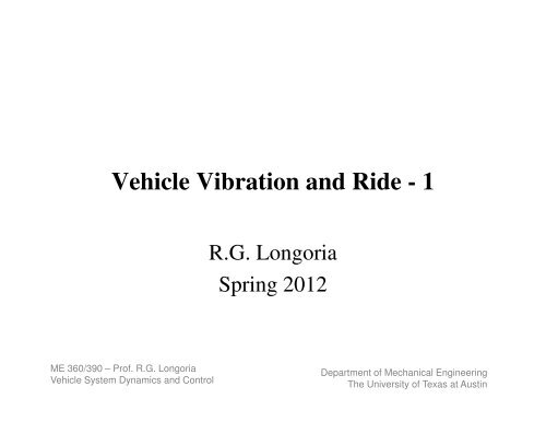
Vehicle Vibration and Ride - Department of Mechanical Engineering ...

Vehicle Vibration and Ride - 1
ME 360/390 – Prof. R.G. Longoria
Vehicle System Dynamics and Control
R.G. Longoria
Spring 2012
Department of Mechanical Engineering
The University of Texas at Austin

ME 360/390 – Prof. R.G. Longoria
Vehicle System Dynamics and Control
Overview
• 1 DOF ¼-car ride model
• Terrain descriptions for vibration
• Random excitation of ¼-car model
• 2DOF ¼-car ride model
• Appendix A (base-excited models)
• Appendix B (human response to vibration)
Department of Mechanical Engineering
The University of Texas at Austin

Sources of Vibration and Noise
Interaction of a ground vehicle with,
– road roughness
– aerodynamic forces
– engine and driveline dynamics
– tire/wheel assembly imbalance dynamics
can induce vehicle body vibration and noise.
ME 360/390 – Prof. R.G. Longoria
Vehicle System Dynamics and Control
Department of Mechanical Engineering
The University of Texas at Austin

ME 360/390 – Prof. R.G. Longoria
Vehicle System Dynamics and Control
Ride and Noise
• Ride quality refers to
– the sensation or feel of the passenger
– tactile and visual vibrations in frequency range from 0 to 25
Hz (low)
• Noise refers to
– aural vibrations
– frequency range 25 to 20,000 Hz (high)
• Ride and noise are perceived differently by humans, so
there is a need to adopt methods that help quantify and
control.
• See Appendix B for more on human response (ref.
Wong, Ch. 7).
Department of Mechanical Engineering
The University of Texas at Austin

A ¼ car model can help build insight
Isolation of the body from the forces generated by the ground unevenness - tire
provides some help in this respect (ride control)
Control of tire normal forces on the ground - by following the ground surface, the tires
will have traction and lateral control (road holding control)
Karnopp and Heess (1991)
ME 360/390 – Prof. R.G. Longoria
Vehicle System Dynamics and Control
Wong (2001)
Department of Mechanical Engineering
The University of Texas at Austin

Key analysis can begin with even simpler system
models illustrating isolation function
You can show that:
The frequency response tells us how the
amplitude or phase of the response will
depend on the frequency of the forcing
function, y(t) (which we can relate to the
terrain profile, y(x), and the forward
velocity, V).
ME 360/390 – Prof. R.G. Longoria
Vehicle System Dynamics and Control
2 2
Z ks + ( ωb)
Zɺ
= =
2 2 2
Y ( k − mω ) + ( bω) Yɺ
Zɺ
Yɺ
Understanding of transfer
functions and frequency
response is essential.
Good isolation
Department of Mechanical Engineering
The University of Texas at Austin

The ¼-car model can provide insight into several
key measures of vehicle ride
These measures are discussed in Wong (2001) and summarized in notes provided
on Vehicle Ride.
Transmissibility Ratio
mus
mass ratio =
m
TR ( 2 ⋅π ⋅f , 0.05)
2
TR ( 2 ⋅π ⋅f , 0.10)
2
TR ( 2 ⋅π ⋅f , 0.20)
2
TR ( 2 ⋅π ⋅f , 0.75)
2
ME 360/390 – Prof. R.G. Longoria
Vehicle System Dynamics and Control
s
0.01
1 . 10 3
1 . 10 4
10
1
0.1
A lighter unsprung mass
provides better vibration
isolation in the midfrequency
range.
Varying mass ratio
0.1 1 10 100
f
Frequency (Hz)
At higher frequencies,
you may ‘feel’ more
with lighter unsprung
mass.
The 1/4 car model is also helpful in introducing the role that controllable or
active elements can play in vehicle suspensions.
Department of Mechanical Engineering
The University of Texas at Austin

Overview of Vibration Models
• 1 DOF: “Base Excitation” – to guide initial
model formulation
• Road surface profiles – to understand how you
specify road-induced excitation
• 2 DOF: ¼-car Model – the ‘standard’ vertical
vibration model
• 2 DOF: Pitch and Bounce Model
ME 360/390 – Prof. R.G. Longoria
Vehicle System Dynamics and Control
Department of Mechanical Engineering
The University of Texas at Austin

1 DOF
2 DOF
Vehicle Vibration Models
ME 360/390 – Prof. R.G. Longoria
Vehicle System Dynamics and Control
2 DOF for pitch and bounce
Department of Mechanical Engineering
The University of Texas at Austin
7 DOF
15 DOF

1 DOF “Base Excitation”
dy dy dx dy
yɺ = = ⋅ = ⋅V
dt dx dt dx
y( x ) = given road profile
ME 360/390 – Prof. R.G. Longoria
Vehicle System Dynamics and Control
Vertical
Vibration:
pɺ = mz ɺɺ = F − mg
z
F = F + F = k x + b( yɺ − zɺ
)
s
s c s s
xɺ = ∆ v = yɺ − zɺ
Note: this variable represents the compression/extension
of the spring element (not its total length).
Department of Mechanical Engineering
The University of Texas at Austin

1 DOF “Base Excitation”
Z k + ( ωb)
=
Y ( k − mω ) + ( bω)
2
s
2
2 2 2
3
mbω
tanψ
=
( k − mω ) + ( bω)
2 2 2
Z
z( t) = ⋅Yo ⋅sin( ωt −ψ
)
Y
y( t) = Y sin( ωt)
o
ME 360/390 – Prof. R.G. Longoria
Vehicle System Dynamics and Control
Z
Y
Frequency Response for Base Excitation
b
ζ =
b
c
These curves show the effect of damping, although all curves go
through,
ω ω =
n
2
See Appendix A.
Ref.: W.T. Thomson, “Theory of Vibration with
Applications”, Prentice-Hall, 1993.
Department of Mechanical Engineering
The University of Texas at Austin

Using the 1 DOF Model
• To use the 1 DOF model, the input forcing
function needs to be specified. This is simply a
function of time.
• Compute amplitude of output given input.
• For a ground vehicle, we’d like to tie the input
to the type of surface being traversed.
• To do this, you need to relate the input to a
description of the ground surface, and you also
need to consider the ground speed.
ME 360/390 – Prof. R.G. Longoria
Vehicle System Dynamics and Control
Department of Mechanical Engineering
The University of Texas at Austin

Description of Road Surface Profiles
Consider a vehicle traveling with constant speed, V.
To travel between two points X apart takes time,
τ =
X V
The wavenumber of the road, γ, is a measure of the
rate of change with respect to distance or length.
In time, we relate period, T, to frequency, ω. In
space, we relate wavenumber, γ, to wavelength, λ.
T
= 2π
ω
[ ω ] = rad
sec
ME 360/390 – Prof. R.G. Longoria
Vehicle System Dynamics and Control
λ = 2π
γ
[ γ ] = rad
m
Units: Units:
‘cycles’/distance
Road profile
A road can then be described by a
spectrum that is a function of
wavenumber.
Department of Mechanical Engineering
The University of Texas at Austin

Forcing Frequency from Road Profile
Now we can see that a spatial cycle of wavelength, λ, is traversed
by a vehicle during a period, T, given by
T = λ
V
But this period, T, is related to frequency, ω, so we can write,
ME 360/390 – Prof. R.G. Longoria
Vehicle System Dynamics and Control
2π 2π ⋅V ⎡2π ⎤
ω = = = V γV
T λ ⎢
=
⎣ λ ⎥
⎦
So you can relate frequency, ω, to a forward vehicle velocity
using the wavenumber-based description of a road profile.
Department of Mechanical Engineering
The University of Texas at Austin

Road Elevation Profile Descriptions
Surveys of roads use power spectral densities
plotted as functions of wavenumber.
Road profiles show a drop with spatial
frequency, as shown here.
How do you interpret this graph?
What kind of change do you ‘expect’ to see in
front of you over the next inch/cm, foot/m, or
mile?
Could you look at a graph like this and say:
“For my vehicle, this environment will be no
problem.” ?
ME 360/390 – Prof. R.G. Longoria
Vehicle System Dynamics and Control
γ = 2π
λ
Gillespie (1992)
What if this was flat?
Department of Mechanical Engineering
The University of Texas at Austin

Wong (2001)
Road Descriptions as PSD
For high γ
you can get
high
variations.
Note, Wong uses Ω here instead of γ.
ME 360/390 – Prof. R.G. Longoria
Vehicle System Dynamics and Control
You can develop basic functions to
quantify these spectra.
For example, S ( γ ) C γ −
=
g sp
For vehicle vibration, you can
convert this to units of frequency
by the relation,
Department of Mechanical Engineering
The University of Texas at Austin
N
1
Sg ( f ) = Sg
( γ )
V

Data for Road PSD Functions
S ( γ ) C γ −
=
g sp
ME 360/390 – Prof. R.G. Longoria
Vehicle System Dynamics and Control
N
From Wong (Chapter 7)
Department of Mechanical Engineering
The University of Texas at Austin

What can you do with all of this?
For a linear system (the vehicle vibration model), you can compute
the response (vibrations) by using the road profile spectrum (with
frequency transformation).
The vibration
S ( f ) = H ( f ) S ( f )
v g
ME 360/390 – Prof. R.G. Longoria
Vehicle System Dynamics and Control
2
Your linear
vibration
model
The input
Then, you can use measures,
such as:
spectrum f2
rms vibration S( f ) df
= ∫
Department of Mechanical Engineering
The University of Texas at Austin
f
1

1 DOF System Base-Excited
ME 360/390 – Prof. R.G. Longoria
Vehicle System Dynamics and Control
by Random Road Input (1)
Consider the base-excited system as a
model of a vehicle being driven over
a road that has a road profile given
by, 2 2
mm 100 mm
Sg ( γ ) = 100 =
cycles/m 2π rad/m
100
2⋅π = 15.915
10 6 ⋅Sg
( γ)
20
10
constant
0
0 1 2
γ
wavenumber
γ =
2π
λ
Z
Y
This PSD is re-written in terms of
angular frequency using,
1 ω
Sg ( ω) = Sg
( γ = )
V V
In this case,
Sg
2
100 1 mm
( ω)
=
2π V rad/s
Department of Mechanical Engineering
The University of Texas at Austin

H ( ω)
n
1 DOF System Base-Excited
ME 360/390 – Prof. R.G. Longoria
Vehicle System Dynamics and Control
by Random Road Input (2)
Use the PSD as input to the transfer
function previously derived and now
expressed in the form,
Let,
2
Z 1 + (2 ςr)
= =
Y (1 − r ) + (2 ςr)
2 2 2
ω c k
r = ; ς = ; ωn
=
ω 2 km m
ω = 2 π (1.5) rad/sec
n
ζ = 0.1
H ( ω)
Hmag2( r)
This is the squared result for this case.
2
5
0
Z
Y
0 2 4
r
Department of Mechanical Engineering
The University of Texas at Austin

Now apply the relation:
10 6 ⋅Sg
( γ)
20
10
0
0 1 2
1 DOF System Base-Excited
ME 360/390 – Prof. R.G. Longoria
Vehicle System Dynamics and Control
by Random Road Input (3)
S ( ω) = H ( ω) S ( ω)
Hmag2( r)
z g
5
0
0 2 4
γ 2
r
S ( ω )
H ( ω)
S ( ω)
g
Assume:
V = 30 km/hr
This is the
power spectral
density (PSD)
of the mass
velocity.
2
10 6 ⋅Sv
( ω )
100
10
1
10 6 ⋅Sv
( ω )
z
100
10
1
0.1
0 10 20
0.1
0 10 20
Department of Mechanical Engineering
The University of Texas at Austin
ω
ω

1 DOF System Base-Excited
ME 360/390 – Prof. R.G. Longoria ω
Vehicle System Dynamics and Control
by Random Road Input (4)
From the response PSD, you can compute the standard deviation and root-meansquare
values.
10 6 ⋅Sv
( ω )
Sz ( ω)
100
10
1
0.1
0 10 20
10 6 ⋅Sv
( ω )
100
10
1
0.1
ω
0 10 20
∞
2
z = ∫ z
0
σ S ( ω) dω
Area under PSD σ v2
RMS
Use “practical” end
points for integration.
⌠
:= ⎮
⌡
20⋅Hza 0⋅Hza Sv( ω)
dω
σv2 150. mm 2
=
σv2 = 12.25 mm
Units: rad/sec
Department of Mechanical Engineering
The University of Texas at Austin

1 DOF System Base-Excited
ME 360/390 – Prof. R.G. Longoria
Vehicle System Dynamics and Control
by Random Road Input (5)
As a continuation, consider now a
road profile described by the
relation, N
S ( γ ) C γ −
=
g sp
For the same example, you will
find the input takes the form
shown to the right. In this case,
for V =
30 km/hr
σv2 21.241mm 2
=
σv2 = 4.609mm
10 6 ⋅Sy
( ω )
10 6 ⋅Sv
( ω )
1 . 10 3
10
1
0.1
0 5 10
100
10
1
0.1
0.01
ω
0 10 20
ω
Department of Mechanical Engineering
The University of Texas at Austin

Example: Problem 7.5 (Wong)
ME 360/390 – Prof. R.G. Longoria
Vehicle System Dynamics and Control
Department of Mechanical Engineering
The University of Texas at Austin

Example: Problem 7.5 (Wong)
ME 360/390 – Prof. R.G. Longoria
Vehicle System Dynamics and Control
Department of Mechanical Engineering
The University of Texas at Austin

ME 360/390 – Prof. R.G. Longoria
Vehicle System Dynamics and Control
Summary
• The base-excited model should be used to understand
the basic vibration problem in a ¼-car vehicle model.
• The transmissibility ratio illustrates the frequency
response of the base-excited mass-spring-damper
system (see also Appendix B).
• Road profiles can be transformed into input forcing
power spectral densities which ‘drive’ the system.
• Basic functions provide a way to estimate the response
spectrum and critical values such as the rms velocity
or acceleration.
• Vehicle ride models can become more complex as you
add the effect of additional masses, etc.
Department of Mechanical Engineering
The University of Texas at Austin

ME 360/390 – Prof. R.G. Longoria
Vehicle System Dynamics and Control
¼ Car Models for Ride
• The ¼ car model is used for modeling the vertical vibration of a
vehicle, taking 1/4 th of the sprung mass and incorporating
associated unsprung mass (effective tire, axle, etc.).
• The mathematical (vibration) model is derived by applying
Newton’s law to each mass, identifying the forces induced on
each mass (see next slide).
• This leads to a 2 degree of freedom (DOF) model.
• For linear analysis, it is convenient to follow the traditional
model, as outlined in Wong and summarized in the following
slides. This analysis utilizes the 2 nd order form of the equations.
• For cases where the suspension elements become nonlinear, or
to study the effect of semi-active or active suspension elements,
it is convenient to formulate the equations as a set of 1 st order
‘state’ equations. These can be used directly in simulation and
or control system analysis.
Department of Mechanical Engineering
The University of Texas at Austin

¼ Car Vehicle Model
2 DOF Model for Sprung and Unsprung Mass
From Wong
For sprung mass:
m ɺɺ z + c ( zɺ − zɺ ) + k ( z − z ) = Vertical Forces on Sprung Mass
s 1 sh 1 2 s 1 2
For unsprung mass:
m ɺɺ z + c ( zɺ − zɺ ) + k ( z − z ) + c zɺ + k z = F( t) = c zɺ + k z
us 2 sh 2 1 s 2 1 t 2 tr 2 1 0 tr 0
ME 360/390 – Prof. R.G. Longoria
Vehicle System Dynamics and Control
Excitations from aerodynamics
and engine and driveline are
applied to sprung mass.
Tire/wheel imbalance forces are
applied to unsprung mass.
How do you find these terms?
Department of Mechanical Engineering
The University of Texas at Austin

Wong, Fig. 7.5
− m ω + k −k
¼ Car Vehicle Model
Finding the Natural Frequencies
s
2
n s s
−ks 2
− msωn + ks + ktr
ME 360/390 – Prof. R.G. Longoria
Vehicle System Dynamics and Control
To find the natural frequencies, take the undamped,
unforced system,
m ɺɺ z + k ( z − z ) = 0
s 1 s 1 2
m ɺɺ z + k ( z − z ) + k z = 0
us 2 s 2 1 tr 2
Assume the response of each variable will take form,
=
0
z = Z cosω
t
1 1
z = Z cosω
t
2 2
Plug into the equations above leads to two equations valid for any Z 1 and Z 2 so long as,
n
n
Characteristic equation
+ 2 natural frequencies.
Department of Mechanical Engineering
The University of Texas at Austin

ω
f
ω
f
n1
n1
n2
n2
¼ Car Vehicle Model
Calculating the Natural Frequencies
4
ω ( m m ) + ω −m k − m k − m k + k k = 0
ME 360/390 – Prof. R.G. Longoria
Vehicle System Dynamics and Control
( )
n s us n s s s tr us s s tr
= 6.563 rad/sec
= 1.045 Hz
= 66.19 rad/sec
=
10.54 Hz
Two solutions:
f
n1,2
ω
ω
2
n1
2
n2
=
=
ωn1,2
=
2π
B − B − 4AC
1
2
1 1 1
2A
B + B − 4AC
1
2
1 1 1
1
1
1
1
2A
1
A = m m
s us
B = m k + m k + m k
C = k k
s s s tr us s
s tr
Department of Mechanical Engineering
The University of Texas at Austin

f
¼ Car Vehicle Model
Approximating the Natural Frequencies
1 1 ksktr 1 RR
− = =
2π m k + k 2π
m
n s
f
n−us =
1
2π
s s tr s
k + k
m
s tr
us
See also Gillespie (1992), p. 148
RR = ride rate
ME 360/390 – Prof. R.G. Longoria
Vehicle System Dynamics and Control
For a typical passenger car, the sprung mass can
be an order of magnitude larger than unsprung
mass, while the suspension stiffness is an order of
magnitude lower than the equivalent tire stiffness.
Case 1: Neglect m us, find equivalent stiffness (RR)
Case 2: Assume vehicle acts like ‘big inertia’ and
mus bounces between ground and inertia
f
f
n−s n−us = 1.045 Hz
= 10.53 Hz
Department of Mechanical Engineering
The University of Texas at Austin

Using ¼ car approximations
• Unsprung mass is often an order of magnitude higher than
sprung mass (for passenger vehicles).
• Damping ratio in shock absorbers is usually in the range 0.2 to
0.4.
• Damping in tire is usually very small.
• You can approximate damped natural frequency with natural
frequency in many cases.
ς =
2
ME 360/390 – Prof. R.G. Longoria
Vehicle System Dynamics and Control
c
km
2
ω = ω 1−
ς
d n
NOTE: With a computer, easy enough to solve these problems, but sometimes it is
good to get ‘feel’ for magnitudes.
Department of Mechanical Engineering
The University of Texas at Austin

Static Deflection vs. Natural Frequency
For ‘standard’ passenger vehicles, you can approximate sprung natural frequency
from static deflection.
10
2
fn− s =
∆
From Gillespie (1992)
ME 360/390 – Prof. R.G. Longoria
Vehicle System Dynamics and Control
f
1 1 k k 1 k
− = ≈
2π m k + k 2π
m
n s
s tr s
s s tr s
1 ks
10
fn− s g
2π
W
≈ ≈ ∆
∆ = static deflection
∆ =
mg
k
Department of Mechanical Engineering
The University of Texas at Austin
ktr >>
ks

Insight into Wheel Hop Resonance
Resonance of the unsprung mass
f
n−us ≐
1
2π
k + k
s tr
m
ME 360/390 – Prof. R.G. Longoria
Vehicle System Dynamics and Control
us
Typical wheel hop resonance
W wheel
m us
:=
:= 100⋅lbf Kt 1000 lbf
:= ⋅ Ks 100
in
lbf
:= ⋅
in
W wheel
g
f n_us
f n_us
:=
1
2⋅π ⋅
K t
= 10.372Hz
+
m us
K s
ς ∝
Gillespie (1992)
Department of Mechanical Engineering
The University of Texas at Austin
1
m

Example: Problem 7.1 (Wong)
ME 360/390 – Prof. R.G. Longoria
Vehicle System Dynamics and Control
NOTE: In 4 th ed., these equation
numbers are 7.20 and 7.21,
respectively.
Department of Mechanical Engineering
The University of Texas at Austin

Example: Problem 7.1 (cont.)
ME 360/390 – Prof. R.G. Longoria
Vehicle System Dynamics and Control
NOTE: In 4 th ed., these equation numbers are 7.22 and 7.24,
respectively.
NOTE: In 4 th ed., these
equation numbers are 7.23 and
7.25, respectively.
Department of Mechanical Engineering
The University of Texas at Austin

Insight from Transfer Functions
Linear transfer functions allow for analysis in the frequency
domain, and the relationships between different variables
provide insight into different suspension characteristics:
• Vibration isolation – response of sprung mass to ground input
• Suspension travel – deflection of suspension spring or relative
displacement between sprung and unsprung mass with respect
to road surface profile
• Road-holding – critically depends on the normal force acting
between the tire and the road surface (dynamic tire deflection)
*Reference Wong, Ch. 7, pp. 442-453
ME 360/390 – Prof. R.G. Longoria
Vehicle System Dynamics and Control
Department of Mechanical Engineering
The University of Texas at Austin

ME 360/390 – Prof. R.G. Longoria
Vehicle System Dynamics and Control
Transfer Functions
for ¼ Car Model - Vibration Isolation 1
Transmissibility Ratio
mus
mass ratio =
m
s
TR ( 2 ⋅π ⋅f , 0.05)
2
TR ( 2 ⋅π ⋅f , 0.10)
2
TR ( 2 ⋅π ⋅f , 0.20)
2
TR ( 2 ⋅π ⋅f , 0.75)
2
0.01
1 . 10 3
1 . 10 4
10
1
0.1
A lighter unsprung mass
provides better vibration
isolation in the midfrequency
range.
Varying mass ratio
0.1 1 10 100
f
Frequency (Hz)
You may ‘feel’ more
higher frequency
vibration with a lighter
unsprung mass.
This is a measure of “vibration isolation”, or the response of the sprung mass to
the excitation from the ground. Here we look at the effect of the ratio of
unsprung to sprung mass (0.05, 0.1, 0.2, 0.75).
Department of Mechanical Engineering
The University of Texas at Austin

ME 360/390 – Prof. R.G. Longoria
Vehicle System Dynamics and Control
Transfer Functions
for ¼ Car Model - Vibration Isolation 2
ktr
stiffness ratio =
k
As expected, a stiffer tire
(relative to suspension)
transmits more force to
sprung mass.
A higher stiffness ratio corresponds to a
softer suspension spring stiffness.
Softer suspension provides better
overall isolation, except in mid region.
s
In this region, you get
better isolation with a
stiffer tire.
Varying stiffness ratio
Department of Mechanical Engineering
The University of Texas at Austin

ME 360/390 – Prof. R.G. Longoria
Vehicle System Dynamics and Control
Transfer Functions
for ¼ Car Model - Vibration Isolation 3
Varying damping
Higher damping is better
in the vicinity of the
natural frequency of the
sprung mass.
In this region, you get
better isolation with
lower damping ratio.
Department of Mechanical Engineering
The University of Texas at Austin

ME 360/390 – Prof. R.G. Longoria
Vehicle System Dynamics and Control
Transfer Functions
for ¼ Car Model - Suspension Travel
( z − z )
This is measured by deflection
of the suspension spring or by
relative displacement of the
sprung and unsprung masses.
Effect of tire to suspension
stiffness is shown.
2 1 max
z
0
Varying stiffness ratio
This helps identify “rattle space”.
At frequencies below
the natural frequency of
the sprung mass, a
softer suspension leads
to higher suspension
travel.
Stiff suspension
Soft suspension
Department of Mechanical Engineering
The University of Texas at Austin

ME 360/390 – Prof. R.G. Longoria
Vehicle System Dynamics and Control
Transfer Functions
for ¼ Car Model - Dynamic Tire Deflection
( z − z )
0 2 max
z
0
Wong (2001)
Not good!
This is a measure of “road holding”, since the dynamic tire deflection ratio
shown is a measure of the normal force on the ground contact.
Light damping
Bad shock
absorber?
Varying damping ratio
Department of Mechanical Engineering
The University of Texas at Austin

ME 360/390 – Prof. R.G. Longoria
Vehicle System Dynamics and Control
Transfer Functions
for ¼ Car Model - Dynamic Tire Deflection
See Problem 7.6
( z − z )
0 2 max
z
0
Wong (2001)
Better vibration isolation with softer suspension, but to get better roadholding
at a frequency of excitation close to the unsprung mass natural
frequency, a stiffer suspension spring should be used.
Varying stiffness ratio
Stiffer suspension
leads to better
road holding.
Department of Mechanical Engineering
The University of Texas at Austin

Example: Problem 7.6 (Wong)
k δ = (total weight)= m g + m g
tr tr s us
2π 2π ⋅V ⎡2π ⎤
ω = = = V γV
T λ ⎢
=
⎣ λ ⎥ V =
f λ
⎦
ME 360/390 – Prof. R.G. Longoria
Vehicle System Dynamics and Control
NOTE: In 4 th ed.,
this is Fig. 7.17.
Department of Mechanical Engineering
The University of Texas at Austin

Example: Off-road axle change
A former student relayed this story:
• He and friends did off-road driving in jeeps.
• A friend changed the standard CJ-7 axle to
heavier Toyota Land Cruiser axles.
• Why would he do that?
• These performed well off-road, but after a year,
the chassis cracked.
• Can you explain why this happened?
ME 360/390 – Prof. R.G. Longoria
Vehicle System Dynamics and Control
Department of Mechanical Engineering
The University of Texas at Austin

Simulation of ¼ Car Model
• We can envision at least two cases where we
must absolutely utilize computer simulation for
the basic ¼ car model:
– To find time-domain response to irregular surface
profiles
– To find response given suspension and/or tire
nonlinearities
• To arrive at the appropriate model, you must:
– Convert the 2 nd order equations into 1 st order form
– Derive directly as 1 st order equations (bond graph?)
ME 360/390 – Prof. R.G. Longoria
Vehicle System Dynamics and Control
Department of Mechanical Engineering
The University of Texas at Austin

1
2
3
3 Ways to Use a ¼ Car Model
Intuitive understanding based on
approximations and knowledge of
natural frequencies and their
relative magnitudes.
Derive and develop transfer
functions between variables of
interest.
Develop differential equations for
direct numerical integration.
ME 360/390 – Prof. R.G. Longoria
Vehicle System Dynamics and Control
Approach Result/Usage
Understanding of the influence of
sprung and unsprung masses, etc., on
suspension performance.
Insight into vibration isolation,
suspension travel, and road holding
capabilities.
Time-domain simulations, allow
nonlinear effects, active system
integration, transient evaluation.
Department of Mechanical Engineering
The University of Texas at Austin

ME 360/390 – Prof. R.G. Longoria
Vehicle System Dynamics and Control
Summary
• Basic 1 and 2 DOF models provide good tools for studying the
dependence of ride performance on component parameter
values.
• Ride analysis focuses on vibrational response of a vehicle to
road excitation, allowing study of the dependence on the
distribution of mass, stiffness, and damping.
• The transfer function models can also show how some
objectives can be at odds with others (introducing the need for
controls).
• It can take time and experience to use basic models effectively,
so nonlinear simulation ends up being a strong tool that can help
overcome difficulties with building insight.
• Later we will examine how active elements and feedback
principles are used in controlled suspensions.
Department of Mechanical Engineering
The University of Texas at Austin

ME 360/390 – Prof. R.G. Longoria
Vehicle System Dynamics and Control
References
1. W.T. Thomson, “Theory of Vibration with Applications”, Prentice-Hall, 1993.
2. Gillespie, T.D., Fundamentals of Vehicle Dynamics, SAE, Warrendale, PA, 1992.
3. Liljedahl, et al, “Tractors and their power units,” ASAE, St. Joseph, MI, 1996.
4. Wong, J.Y., Theory of Ground Vehicles, John Wiley and Sons, Inc., New York,
2001.
5. Karnopp, D. and G. Heess, “Electonically Controllable Vehicle Suspensions,”
Vehicle System Dynamics, Vol. 20, No. 3-4, pp. 207-217, 1991.
Department of Mechanical Engineering
The University of Texas at Austin

ME 360/390 – Prof. R.G. Longoria
Vehicle System Dynamics and Control
Appendix A
Base-excited model and analysis
Department of Mechanical Engineering
The University of Texas at Austin

ME 360/390 – Prof. R.G. Longoria
Vehicle System Dynamics and Control
Appendix A – 1 Ref. Thomson, 1993
Department of Mechanical Engineering
The University of Texas at Austin

ME 360/390 – Prof. R.G. Longoria
Vehicle System Dynamics and Control
Appendix A – 2 Ref. Thomson, 1993
Department of Mechanical Engineering
The University of Texas at Austin

ME 360/390 – Prof. R.G. Longoria
Vehicle System Dynamics and Control
Appendix A – 3
b
ζ =
b
c
Ref. Thomson, 1993
Department of Mechanical Engineering
The University of Texas at Austin

ME 360/390 – Prof. R.G. Longoria
Vehicle System Dynamics and Control
Appendix B
Human response to vibration
Department of Mechanical Engineering
The University of Texas at Austin

Human Response and Perception
• Subjective ride measurements
• Shaker table tests (mostly sinusoidal,
multidirectional)
• Ride simulator tests - can induce
multidirectional vehicle motion
• Ride measurements in vehicles
ME 360/390 – Prof. R.G. Longoria
Vehicle System Dynamics and Control
Department of Mechanical Engineering
The University of Texas at Austin

Vertical Vibration
Limits
From Ride and Vibration Data
Manual (SAE).
“Janeway’s comfort criterion” -
based on sinusoidal vibration
(single frequency)
1-6 Hz: “jerk” should not exceed 12.6
m/s 3 .
6-20 Hz: peak acceleration less than 0.33
m/s 2
20-60 Hz: peak velocity less than 2.7
mm/s
ME 360/390 – Prof. R.G. Longoria
Vehicle System Dynamics and Control
Wong (2001)
Department of Mechanical Engineering
The University of Texas at Austin

ME 360/390 – Prof. R.G. Longoria
Vehicle System Dynamics and Control
Standards: ISO 2631
• For evaluation of vibrational environments in
transport vehicles and in industry.
• Three distinct limits are defined for whole-body
vibration in 1 to 80 Hz frequency range.
– Exposure limits (safety related)
– Fatigue or decreased proficiency (efficiency)
– Reduced comfort
Department of Mechanical Engineering
The University of Texas at Austin

Vertical vibration
ME 360/390 – Prof. R.G. Longoria
Vehicle System Dynamics and Control
ISO 2631
Transverse vibration
Department of Mechanical Engineering
The University of Texas at Austin

ME 360/390 – Prof. R.G. Longoria
Vehicle System Dynamics and Control
Octave Bands
1 Octave bands are geometrically related by the recursive relation, 2 k n+
=
Where the two frequencies, f n and f n+1 are successive band limits (lower and upper),
and the index k is a positive integer or a fraction according to a whole octave or
fractional octave.
For example, if k = 1, the ratio between successive bands is 2. If k = 1/3, then the
ratio between the upper and lower band limits is 1.26.
Associated with each band is a center frequency, fc, which is given by the geometric
mean,
f = f f
c n+ 1 n
An octave bandwidth is,
f f BW
n+ 1 − n = (bandwidth)
Contrast this with a decade. If you advance a decade, it is a 10-times increase.
f
f
Department of Mechanical Engineering
The University of Texas at Austin
n

Other Issues and Definitions
• Below 1 Hz exposure leads to motion sickness,
so different standards are set for 0.1 to 1 Hz.
• Absorbed power is a common standard, found
by product of vibration force and velocity
transmitted to human body.
• Absorbed power is used especially in
specifying military vehicle vibration tolerance
levels. For example, 6 W is sometimes referred
to as the maximum amount a human can be
exposed to (and still do their job).
ME 360/390 – Prof. R.G. Longoria
Vehicle System Dynamics and Control
Department of Mechanical Engineering
The University of Texas at Austin

Vehicle Ride Transfer Functions
From Bekker (1969)
ME 360/390 – Prof. R.G. Longoria
Vehicle System Dynamics and Control
h=Hinterseite=front, v = Vorderseite=rear
Department of Mechanical Engineering
The University of Texas at Austin