Guidance for Evaluation of Potential Groundwater Mounding ...

This report by Poeter et al. (2005) contains an error in the 

section on vadose-zone mounding. In the report, the figure and 

equations mistakenly use the full width (W) in place of the halfwidth, 

w, which should have been used. The vadose-zone layer 

examples in the report that demonstrate calculation and use of a 

maximum infiltration-area width, actually represent a maximum 

half width for a given Hmax. The methodology example in the 

report is still correct, however. The full width W was and should 

be used for design calculations. The terminology and equations 

for the saturated zone mounding in the report are not affected by 

this correction. 

NDWRCDP, Washington University, Campus Box 1150 

One Brookings Drive, Cupples 2, Rm. 11, St. Louis, MO 63130-4899

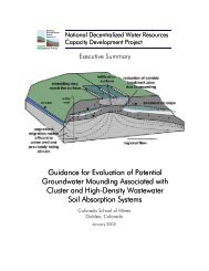
National Decentralized Water Resources 

Capacity Development Project 

Guidance for Evaluation of Potential 

Groundwater Mounding Associated with 

Cluster and High-Density Wastewater 

Soil Absorption Systems 

Colorado School of Mines 

Golden, Colorado 

January 2005

Guidance for Evaluation of Potential 

Groundwater Mounding Associated with 

Cluster and High-Density Wastewater Soil 

Absorption Systems 

Submitted by International Groundwater 

Modeling Center of Colorado School of 

Mines, Golden, Colorado 

NDWRCDP Project Number WU-HT-02-45 

National Decentralized Water Resources Capacity Development Project 

(NDWRCDP) Research Project 

Final Report, January 2005 

NDWRCDP, Washington University, Campus Box 1150 

One Brookings Drive, Cupples 2, Rm. 11, St. Louis, MO 63130-4899

DISCLAIMER 

This work was supported by the National Decentralized Water Resources Capacity Development 

Project (NDWRCDP) with funding provided by the U.S. Environmental Protection Agency through a 

Cooperative Agreement (EPA No. CR827881-01-0) with Washington University in St. Louis. This report 

has not been reviewed by the U.S. Environmental Protection Agency. This report has been reviewed by 

a panel of experts selected by the NDWRCDP. The contents of this report do not necessarily reflect the 

views and policies of the NDWRCDP, Washington University, or the U.S. Environmental Protection 

Agency, nor does the mention of trade names or commercial products constitute endorsement or 

recommendation for use.

CITATIONS 

This report was prepared by 

Eileen Poeter, John McCray, Geoffrey Thyne, and Robert Siegrist 

International Groundwater Modeling Center 

Colorado School of Mines 

Golden, Colorado 80401 

The final report was edited and produced by ProWrite Inc., Reynoldsburg, OH. 

This report is available online at www.ndwrcdp.org. This report is also available through the 

National Small Flows Clearinghouse 

P.O. Box 6064 

Morgantown, WV 26506-6065 

Tel: (800) 624-8301 

WWCDRE46 

This report should be cited in the following manner: 

Poeter E., J. McCray, G. Thyne, and R. Siegrist. 2005. Guidance for Evaluation of Potential 

Groundwater Mounding Associated with Cluster and High-Density Wastewater Soil Absorption 

Systems. Project No. WU-HT-02-45. Prepared for the National Decentralized Water Resources 

Capacity Development Project, Washington University, St. Louis, MO, by the International 

Groundwater Modeling Center, Colorado School of Mines, Golden, CO. 

iii

ACKNOWLEDGEMENTS 

Appreciation is extended to the following individuals for assistance in the preparation of this 

report: 

International Groundwater Modeling Center 

Eileen Poeter, John McCray, Geoffrey Thyne, and Robert Siegrist 

Appreciation is also expressed to the NDWRCDP for their support of this work: 

Principal Investigator 

Jay R. Turner, D.Sc., Washington University 

Project Coordinator 

Andrea L. Shephard, Ph.D. 

NDWRCDP Project Steering Committee: 

Coalition for Alternative Wastewater 

Treatment 

Valerie I. Nelson, Ph.D. 

Consortium of Institutes for Decentralized 

Wastewater Treatment 

Ted L. Loudon, Ph.D., P.E. 

Electric Power Research Institute 

Raymond A. Ehrhard, P.E. 

Tom E. Yeager, P.E. 

National Onsite Wastewater Recycling 

Association 

Jean Caudill, R.S. 

National Rural Electric Cooperative 

Association 

Steven P. Lindenberg 

Scott Drake, P.E. 

Water Environment Research Foundation 

Jeff C. Moeller, P.E. 

Members-At-Large: 

James F. Kreissl 

Richard J. Otis, Ph.D., P.E. 

Jerry Stonebridge 

v

ABSTRACT 

Hydrologic evaluation of cluster and high-density wastewater soil absorption systems (WSAS) is 

important because it can help ensure that a site has sufficient capacity to assimilate water in 

excess of natural infiltration. Insufficient capacity may result in significant groundwater 

mounding on low hydraulic conductivity lenses or elevate the water table, which may alter 

saturated flow direction or reach the surface. Insufficient capacity can also cause lateral 

movement of water, which may affect nearby water supplies or water bodies or cause effluent 

breakout on slopes in the vicinity. Practitioners and stakeholders must be informed of the issues 

so they will be able to complete the proper investigations and evaluations. Most critical is 

evaluation of the potential for reduction of the vadose zone thickness, which could result in 

inadequate retention times and conditions for treatment of wastewater pollutants. This report 

presents a methodology for: 

• Evaluation of site-conditions and system-design influences on the potential for groundwater 

mounding and lateral spreading 

• Selection of investigation techniques and modeling approaches based on site conditions, 

system parameters, and the severity of the consequences of excessive mounding 

A flow chart and decision-support tool are provided to determine the strategy-level for site 

investigation and model evaluation depending on the potential for groundwater mounding and 

the consequences should it occur. Characterization activities and modeling approaches, 

appropriate for each level of assessment are delineated. 

vii

EXECUTIVE SUMMARY 

Cluster and high-density wastewater soil-absorption systems (WSAS) (those receiving more than 

2,000 gallons of water per day or GPD) are increasingly required to serve development. In the 

past, system designers and regulators focused on vertical movement of water from WSAS 

because most systems are small and isolated. However, insufficient capacity may result in (see 

Figure ES-1): 

• Significant groundwater mounding on low hydraulic conductivity lenses or elevation of the 

water table (which may alter saturated flow direction or reach the surface) 

• Lateral movement of water, which may affect nearby water supplies or water bodies, or may 

cause effluent breakout on slopes in the vicinity 

Rationale and Purpose 

For the purpose of this report, failure is considered to be excessive mounding. Some mounding 

will not cause hydraulic breakout at the surface or side slopes or insufficient treatment of the 

wastewater, but may impact performance efficiency of the WSAS, or cause the system to be out 

of compliance with local regulations. This report focuses on the methodology for determining the 

magnitude of mounding, vertically and laterally. Once that magnitude is known, the designer 

must determine whether the WSAS function will be acceptable based on treatment requirements 

and local regulations. 

Figure ES-1 

Potential Groundwater Mounding Below WSAS 

ix

Hydrologic evaluation is important because it ensures a site has sufficient hydraulic capacity to 

assimilate water in excess of natural infiltration. Practitioners and stakeholders must be informed 

of the issues so they will be able to complete the proper investigations and evaluations. Most 

critical is evaluation of the potential for reduction of the vadose (unsaturated) zone thickness, 

which could result in inadequate retention times and conditions for treatment of wastewater 

pollutants. 

This report presents a methodology for: 





Methodology 

Evaluation of the potential for groundwater mounding and break-out on the surface or side slopes 

requires different levels of effort depending on the characteristics of the subsurface and the 

consequences of system failure. The phased approach indicates more investigation as the risk of 

mounding increases and the consequences of failure due to mounding become more severe. A 

flowchart guides preliminary assessment and indicates subsequent steps, based on preliminary 

site investigation to determine depth to groundwater and soil types (Figure ES-2). Specific 

sections of the report elaborate on these steps. 

x 

Sections: 3.5.1.4 & 3.6.1.4 

Sections: 3.5.5 & 3.6.5 

Figure ES-2 

Flowchart for Preliminary Assessment of the Potential for Groundwater Mounding Guides 

Subsequent Steps of the Assessment Process

Decision-Support Tool 

A decision-support tool quantifies a subjective strategy level that defines the intensity of site 

characterization and modeling appropriate for a given site, following the philosophy that the 

degree of characterization and associated cost should be considered in light of the potential for 

mounding and the consequences should mounding occur. The decision-support tool utilizes 

additional qualitative information relative to the flowchart as well as site-specific quantitative 

data from field investigations to determine the strategy level for site assessment. The strategy 

level provides a guide to the magnitude and intensity of field investigation and the sophistication 

of modeling. Guidance on site investigation is provided in Chapter 2, while guidance on 

modeling is presented in Chapter 3 of this report. Associated costs of field investigations and 

model assessment are discussed at the end of Chapters 2 and 3. 

Levels of Site Investigation 

Sites with hydraulic conditions that indicate low risk of mounding, and have minimal 

consequences in the case of mounding, can be assessed using minimal site investigation 

(Chapter 2, sections 2.2 through 2.4) and using analytical solutions to estimate mound height 

(Chapter 3, sections 3.5.1 through 3.5.4 for evaluation of vadose zone mounding; and sections 

3.6.1 through 3.6.4 for saturated zone modeling). Spreadsheets for evaluating mounding of the 

water table (WaterTableMounding_EnglishUnits.xls or WaterTableMounding_SIUnits.xls) are 

available electronically with this report on the CD and online at www.ndwrcdp.org. In these 

low-risk cases, the estimated height of mounding is added to the high water table to determine if 

the design will be acceptable. 

Sites with hydraulic conditions that indicate risk of mounding, and where the consequences of 

mounding are severe, require more intense field investigations (Chapter 2, sections 2.5 and 2.6) 

and sophisticated numerical models to estimate mound height (Chapter 3, section 3.5.5 for 

evaluation of vadose zone mounding of water on low hydraulic conductivity layers; and section 

3.6.5 for mounding of the water table based on flow in the saturated zone). Advanced assessment 

is particularly important for sites where mounding has serious consequences, and sites that 

exhibit strong heterogeneity and/or anisotropy, sites with complicated boundary conditions, and 

those with significant time-varying hydraulic conditions. 

Hydraulic Conductivity of the Soil And Aquifer 

For evaluation of mounding, the most significant factor is the hydraulic conductivity of the soil 

and aquifer, as indicated by example calculations presented in this report. Accurate measurement 

of hydraulic conductivity (K) is difficult because its value varies substantially over short 

distances due to heterogeneity. Therefore, careful attention must be given to this important 

parameter. 

xi

Hydraulic conductivity cannot be accurately estimated from simply knowing the soil type 

because K of a given soil type may vary by orders of magnitude. Therefore, obtaining reliable 

measurements of K when performing engineering analysis for cluster systems is important. 

Suggested methods for measurement of K in unsaturated and saturated soil are outlined in 

Chapter 2, section 2.6. Errors on the order of a factor of 10 would not be unusual; even when 

site-specific measurements are collected. 

Analyzing the statistics on several measurements provides insight on the error associated with K 

measurements. If the designer has not collected detailed measurements of K, but has obtained a 

reasonable estimate based on soil classification or a few measurements, then the site should be 

evaluated using a range of K, including the expected value and a factor of 10 above and, most 

importantly, below the expected value for estimating mound height. 

Analytical and Numerical Modeling 

Whether the assessment requires analytical or numerical modeling, the designer must consider 

two possibilities: 

• Wastewater may mound on low hydraulic conductivity layers in the vadose zone 

• Wastewater may cause mounding of the water table beneath the infiltration area or the 

perched mound 

Analytical models provide estimates of both types of mounding with little investment of the 

designer’s time. If the analyses use conservative parameter values and the results indicate 

mounding is not excessive, then more expensive and time-consuming analyses are not required. 

Limitations of analytical models should be recognized so that conservative parameter values can 

be selected. These limitations are summarized in the following section. Guidance on coping with 

the limitation is provided in this report. The limitations include: 

• The analytical solutions provided for estimating mounding on a low hydraulic conductivity 

layer in the vadose zone do not consider unsaturated-flow physics due to the computational 

complications such consideration would generate. Consideration of these processes would 

delay the time of mound development, but decrease its magnitude; thus their omission is 

reasonable. 

• The analytical solutions do not account for anisotropic hydraulic conductivity. Hydraulic 

conductivity, K, is a soil property describing how easily water flows through the soil. 

Anisotropy is the situation where K varies with direction. Generally the vertical hydraulic 

conductivity is less than the horizontal; however, the reverse is sometimes found in soil 

deposited by wind. 

xii

• The analytical solutions do not account for heterogeneity. Heterogeneity is the variation of K 

in space. If heterogeneities are randomly distributed, then the best value to use for K is the 

geometric mean of the various K values. However, collecting sufficient data for a reasonable 

assessment of the geometric mean is unfeasible. Thus, a conservative (low) value for K must 

be chosen, probably based on the results of several spatially variable estimates or 

measurements of K. If a discontinuous layer exists, then assuming the layer is continuous 

would provide a conservative estimate (over prediction) of the mound height and extent 

because some of the wastewater would travel between the discontinuous low-K zones and 

would not mound in these areas. For severely heterogeneous systems, several pilot-scale 

infiltration tests should be conducted. 

• The analytical solutions do not consider the possibility of heavy rainfall causing short-term 

increased mounding. To address this issue, one needs to use a numerical model that can 

simulate transient, unsaturated flow. However, as a conservative assumption, the designer 

could assume that the mound height would increase by the total rainfall accumulated during 

the storm divided by porosity of the soil. A more reasonable estimate could be obtained by 

subtracting an estimated amount for runoff. 

Although simplifying assumptions are made when using analytical models, expediency warrants 

their use before numerical modeling is considered. When there is potential for problematic 

mounding as judged by preliminary assessment and design changes cannot sufficiently reduce 

that potential, then use of a numerical model is appropriate. Setting up numerical models for a 

specific site is time consuming and requires a significant level of expertise in hydrology, soil 

physics, numerical methods, and computer operation, and is therefore quite expensive. However, 

if the risks associated with excessive mounding are serious, the expense may be worth the effort. 

Getting Started 

Practitioners seeking to utilize the methods presented in this report can best accomplish this by 

working through the recommendations of Chapter 2, Site Evaluation for Groundwater Mounding 

Potential and moving on to sections of Chapter 3, Evaluating Groundwater Mounding With 

Models as needed. 

The first consideration in design of a large system is to specify an overall size of the infiltration 

area that, when coupled with the anticipated volumetric loading rate, results in an infiltration rate 

that is less than the vertical hydraulic conductivity of the soil to prevent the development of 

ponding of wastewater over the infiltration area. That is: 

Q 

A 

< Kv 

for consistent dimensional units of volume, length, and time. Next, recognizing spatial 

constraints of the site and reasonable dimensions for construction, strive to elongate the 

infiltration area in the direction perpendicular to groundwater flow beneath the site. Preliminary 

data acquisition as outlined in Chapter 2, Site Evaluation for Groundwater Mounding Potential, 

will provide approximate values for Kv and flow direction. 

xiii

After establishing this reasonable design, the designer must consider the potential for perching 

and mounding of water on low hydraulic conductivity layers in the vadose zone and ultimately 

the rise of the water table required to carry the wastewater away from the site. Site-scale 

hydraulic conductivities are extremely important to performance of the WSAS, but are difficult 

to determine with certainty. Chapter 2, Site Evaluation for Groundwater Mounding Potential, 

guides the designer in evaluating the amount and type of field investigation appropriate for a site 

and refers the designer to Chapter 3, Evaluating Groundwater Mounding With Models for 

analytical, and if necessary, numerical modeling. 

The analytical modeling recommended in this report is readily accomplished using a calculator 

in the case of estimating mounding on low hydraulic conductivity layers in the vadose zone, and 

the spreadsheets that accompany the report (WaterTableMounding_EnglishUnits.xls or 

WaterTableMounding_SIUnits.xls) in the case of water table mounding of the saturated zone. 

Unless the designer is knowledgeable in the area of numerical modeling, he or she will likely 

enlist a modeler to assist with the work. In spite of this, the sections on numerical modeling 

(Chapter 3, sections 3.5.5 and 3.6.5) are recommended reading because they are not directions on 

how to conduct numerical modeling, but rather illustrations of how mounding is likely to vary 

for conditions that cannot be evaluated with analytical models. The insight they provide is useful 

to all phases of investigation and design. Hypothetical site dimensions and conditions are 

evaluated to illustrate generic system responses. Actual values of mound height and extent can 

only be determined for site-specific properties, dimensions, and boundary conditions. 

xiv

TABLE OF CONTENTS 

1 INTRODUCTION................................................................................................................1-1 

1.1 Rationale...........................................................................................................................1-1 

1.2 Purpose ..............................................................................................................................1-2 

1.3 Methodology .....................................................................................................................1-2 

1.4 Background.......................................................................................................................1-3 

1.4.1 Wastewater Treatment by WSAS...............................................................................1-3 

1.4.2 WSAS Failure.............................................................................................................1-4 

1.4.3 WSAS Case Studies ..................................................................................................1-5 

1.5 Methods for Evaluating Potential Groundwater Mounding ...............................................1-8 

2 SITE EVALUATION FOR GROUNDWATER MOUNDING POTENTIAL ..........................2-1 

2.1 Getting Started..................................................................................................................2-1 

2.2 Determination of the Level of Required Evaluation ..........................................................2-3 

2.3 Existing Data and Site Visit.............................................................................................2-10 

2.4 Preliminary Evaluation....................................................................................................2-10 

2.5 Site Observations ...........................................................................................................2-11 

2.6 Subsurface Investigation ................................................................................................2-12 

2.7 Advanced Hydrologic Testing .........................................................................................2-16 

2.8 Characterization Costs ...................................................................................................2-18 

2.9 Application to Case Studies............................................................................................2-19 

3 EVALUATING GROUNDWATER MOUNDING WITH MODELS ......................................3-1 

3.1 Challenges of Quantitative Estimating..............................................................................3-1 

3.2 Analytical Models..............................................................................................................3-1 

3.3 Numerical Models.............................................................................................................3-2 

xv

3.4 Preliminary Modeling Considerations ...............................................................................3-5 

3.5 Estimating Mounding on a Low Hydraulic Conductivity Layer in the Vadose Zone 

Below a Wastewater Infiltration Area......................................................................................3-5 

3.5.1 Khan et al. (1976) Analytical Solution.........................................................................3-7 

3.5.2 Discussion of Analytical-Solution Results...................................................................3-9 

3.5.3 Designing Wastewater Infiltration Areas for Cluster Systems with Respect to 

Groundwater Mounding in the Vadose Zone Using Analytical Modeling...........................3-12 

3.5.4 Limitations of Analytical Modeling ............................................................................3-18 

3.5.5 Numerical Solutions .................................................................................................3-20 

3.6 Estimating Mounding of the Water Table Below a Wastewater Infiltration Area.............3-30 

3.6.1 Hantush (1967) Analytical Solution ..........................................................................3-31 

3.6.2 Discussion of Analytical-Solution Results.................................................................3-34 

3.6.3 Designing Wastewater-Infiltration Areas for Cluster Systems Using Analytical 

Modeling............................................................................................................................3-39 

3.6.4 Limitations of Analytical Modeling ............................................................................3-45 

3.6.5 Numerical Modeling..................................................................................................3-47 

3.7 Model Acquisition and Implementation ...........................................................................3-60 

3.7.1 Model Implementation ..............................................................................................3-61 

3.7.2 Modeling Costs.........................................................................................................3-61 

4 SUMMARY.........................................................................................................................4-1 

4.1 Hydrologic Evaluation .......................................................................................................4-1 

4.2 Decision-Support Tool ......................................................................................................4-2 

4.3 Hydraulic Conductivity of the Soil and Aquifer..................................................................4-2 

4.4 Analytical and Numerical Modeling...................................................................................4-3 

4.4.1 Analytical Modeling ....................................................................................................4-4 

4.4.2 Numerical Modeling ......................................................................................................4-4 

4.4.3 Limitations of Analytical Modeling ..............................................................................4-4 

5 REFERENCES...................................................................................................................5-1 

xvi

A DEFINITIONS.................................................................................................................. A-1 

Acronyms and Abbreviations................................................................................................. A-1 

Technical Terms .................................................................................................................... A-2 

Frequently Used Variables .................................................................................................... A-6 

B NUMERICAL UNSATURATED FLOW CODES ............................................................. B-1 

xvii

LIST OF FIGURES 

Figure 1-1 Issues of Concern That Can Be Addressed With a Hydrogeologic Evaluation. .......1-1 

Figure 2-1 Flowchart for Preliminary Evaluation of Site Characterization Requirements ..........2-3 

Figure 2-2 USDA Soil Classification by Grain Size....................................................................2-4 

Figure 2-3 A Broad Distribution of Boreholes and Trenches Provides an Overview of the 

Magnitude of Heterogeneity at the Site............................................................................2-15 

Figure 3-1 Conceptual Diagram of Mounding Below WSAS......................................................3-2 

Figure 3-2 Infiltration Area Subunit Layout Concept ..................................................................3-3 

Figure 3-3 Conceptual Model for the Khan Analytical Solution (Khan et al. 1976) ....................3-6 

Figure 3-4 Maximum Infiltration Area Width (W max) 

Versus Maximum Mound Height 

(H max) for Coarse Sand (K 1= 

164 ft/day, 50 m/day) Over Two Different Types of 

Low-K Soil (Silty-Clay and Marine Clay) ............................................................................3-9 

Figure 3-5 Maximum Infiltration Area Width (W max) 

Versus Maximum Mound Height 

(H max) for Silt (K 1= 

0.164 ft/day, 0.05 m/day) Over Two Different Types of Low-K 

Soil (Silty-Clay and Marine Clay) .......................................................................................3-9 

Figure 3-6 General Nomograph for Estimating Maximum Infiltration Area Width From 

Subsurface Properties......................................................................................................3-11 

Figure 3-7 Maximum Infiltration Area Width (Wmax) Versus Depth to the Low-K Layer at 

the Slope Location for Sandy-Loam (K 1) Over Silty-Clay (K 2 ) ..........................................3-12 

Figure 3-8 General Nomograph for Determining Maximum Infiltration Area Width and 

Infiltration Rate (q') for the Design Example in Table 3-2.................................................3-17 

Figure 3-9 Finite-Element Mesh Used for HYDRUS-2D Modeling...........................................3-23 

Figure 3-10 Soil Distribution for Model Cases 1 and 3 ............................................................3-23 

Figure 3-11 Analytical Versus Numerical Solution for Model Case 1 ......................................3-24 

Figure 3-12 Pressure-Head (m of water) Profile Along the Top of the Low-K Layer (3 m 

[approximately 10 ft] below infiltration area) for Model Case 1 ........................................3-24 

Figure 3-13 Pressure-Head Distribution for Model Case 1, 20 Days After Starting 

Infiltration (top), and 200 Days (steady state) After Starting Infiltration (bottom) .............3-25 

Figure 3-14 Soil Distribution for Model Case 2. .......................................................................3-26 

Figure 3-15 Pressure-Head (m of water) Profile Along the Top of the Low-K Layer for 

Model Case 2 ...................................................................................................................3-26 

Figure 3-16 Pressure-Head Distribution for Model Case 2, 200 Days (steady state) After 

Starting Infiltration ............................................................................................................3-27 

Figure 3-17 Pressure-Head Profile for Model Case 3 (2:1 anisotropy), 150 Days After 

Starting Infiltration (near steady state) .............................................................................3-28 

Figure 3-18 Analytical Versus Numerical Solutions for Mounding for Cases 1 and 3..............3-28 

xix

Figure 3-19 Pressure-Head Distribution for Model Case 3, 200 Days (steady state) After 

Infiltration Begins..............................................................................................................3-29 

Figure 3-20 Comparison of Numerical Solutions for 2:1 Anisotropic Case with Two 

Modified Analytical Solutions ...........................................................................................3-29 

Figure 3-21 Conceptual Model for Hantush (1967) Solution....................................................3-33 

Figure 3-22 Evaluate Breakout on a Nearby Side Slope at x 1, y1 

............................................3-33 

Figure 3-23 Mounding as a Function of Saturated Thickness (distance from water table 

to aquifer bottom, Figure 3-21) for Specified Effective Infiltration Rate and K = 0.05 

m/day ...............................................................................................................................3-35 

Figure 3-24 Mounding as a Function of Saturated Thickness for Specified Effective 

Infiltration Rate and K = 0.5 m/day...................................................................................3-36 


Infiltration Rate and K = 5 m/day......................................................................................3-36 


Infiltration Rate and K = 50 m/day....................................................................................3-37 

Figure 3-27 Mounding as a Function of Saturated Thickness for Specified Number of 

Subunits and K = 0.05 m/day ...........................................................................................3-37 


Subunits and K = 0.5 m/day.............................................................................................3-38 


Subunits and K = 5 m/day................................................................................................3-38 


Subunits and K = 50 m/day ..............................................................................................3-39 

Figure 3-31 Example Problem Site Dimensions and Slope Position .......................................3-40 

Figure 3-32 Example Problem in Spreadsheet: a) Overview b) Close Up of Calculations ......3-43 

Figure 3-33 First Conceptual Model for Numerical Modeling (horizontal water table 

without natural recharge or lateral regional flow) .............................................................3-49 

Figure 3-34 Second Conceptual Model for Numerical Modeling (sloping water table with 

natural recharge, and thus lateral regional flow) ..............................................................3-50 

Figure 3-35 First Conceptual Model Solved for the Isotropic Case Evaluated in the 

Example from Section 3.6.3 .............................................................................................3-52 

Figure 3-36 First Conceptual Model (Figure 3-21) With Twice the Distance Between the 

Constant Head Boundaries, Solved for the Isotropic Case Evaluated in the Example 

from Section 3.6.3 ............................................................................................................3-53 

Figure 3-37 First Conceptual Model (Figure 3-21) With Varying K for the Isotropic and 

Anisotropic (Kh:K v = 10:1) Cases.....................................................................................3-54 

Figure 3-38 Second Conceptual Model (Figure 3-22) With Varying K for the Isotropic and 

Anisotropic (Kh:Kv = 10:1 and 100:1) Cases for High and Low Gradients Achieved 

by Varying Recharge........................................................................................................3-56 

Figure 3-39 Second Conceptual Model (Figure 3-22) With Saturated Thickness of 32.8 ft 

(10 m), K = 16.4 ft/d (5 m/d), and 100:1 Anisotropy .........................................................3-57 

Figure 3-40 Second Conceptual Model (Figure 3-22) With Saturated Thickness of 65.6 ft 


Figure 3-41 Second Conceptual Model (Figure 3-22) With Saturated Thickness of 164 ft 


xx

LIST OF TABLES 

Table 1-1 List of Case Studies Reviewed to Identify Useful Examples for This Report.............1-5 

Table 1-2 Basic Parameter Values Used in Quantitative Case Studies ....................................1-8 

Table 2-1 Methodology for Subjective Evaluation of the Potential for Perching, Water 

Table Mounding, or Breakout on Slopes............................................................................2-5 

Table 2-2 Methodology for Subjective Evaluation of the Consequences Should the 

System Fail ........................................................................................................................2-6 

Table 2-3 Methodology for Subjective Evaluation of the Strategy Level for Site 

Investigation and Modeling ................................................................................................2-7 

Table 2-4 Intensity of Field Investigation for Each Strategy Level .............................................2-7 

Table 2-5 Sophistication of Model Evaluation for Each Strategy Level .....................................2-9 

Table 3-1 Design Procedure Considering Mounding on Low-Conductivity Layers in the 

Vadose Zone....................................................................................................................3-14 

Table 3-2 Example Design Application Considering Mounding on Low-Conductivity 

Layer in the Vadose Zone ................................................................................................3-15 

Table 3-3 van Genuchten Parameters used in HYDRUS-2D ..................................................3-22 

Table 3-4 Design Procedure Considering Mounding of the Water Table on Low- 

Hydraulic Conductivity Layers in the Vadose Zone..........................................................3-41 

Table 3-5 Example Application of Design Procedure Considering Mounding of the Water 

Table ................................................................................................................................3-44 

Table 3-6 Costs Associated With Evaluation of Groundwater Mounding Using Numerical 

Models Based on Level of Expertise................................................................................3-63 

xxi

1 INTRODUCTION 


2,000 gallons per day, GPD) are increasingly required to serve development. In the past, system 

designers and regulators focused on vertical movement of water from WSAS because most 

systems are small and isolated. However, increased use of high-density or cluster WSAS requires 

hydrogeologic evaluation to help ensure the site has sufficient capacity to accept the design flow 

in addition to the natural infiltration without: 

• Resulting in groundwater mounding on low hydraulic conductivity (K) lenses or by elevating 

the water table (which may alter flow directions or cause groundwater to reach the surface) 


cause effluent breakout on slopes in the vicinity (Figure 1-1) 

Figure 1-1 

Issues of Concern That Can Be Addressed With a Hydrogeologic Evaluation. 

1.1 Rationale 

Hydrologic evaluation is important because it ensures that a site has sufficient capacity to 

assimilate water in excess of natural infiltration. Practitioners and stakeholders must be informed 

of the issues so they will be able to complete the proper investigations and evaluations. Most 

critical is the evaluation of the potential for reduction of vadose zone thickness, which could 

result in inadequate conditions for treatment of wastewater pollutants. 

1-1

Introduction 

1.2 Purpose 

The purpose of this document is to provide guidance on evaluation of the magnitude of 

mounding, which may cause breakout of groundwater above or adjacent to large cluster and 

high-density WSAS such as those that may serve clusters of homes, resorts, small communities, 

apartment and condominium complexes, and have daily flow volumes 10 or more times greater 

than individual systems. This document specifically does not address the long-term acceptance 

rate (LTAR) of the WSAS trenches. For discussion of LTAR, refer to Siegrist (1987) and 

Siegrist et al. (2001). 

This report presents methodology for determining the magnitude of mounding, vertically and 

laterally. Once that magnitude is known, the designer must determine whether the WSAS 

function will be acceptable based on treatment requirements and local regulations. 

1.3 Methodology 

This report presents a methodology for: 





Methodology for site investigation and evaluation of the potential for groundwater mounding as 

perched zones or as a rise in the water table is presented in Chapter 2, Site Evaluation for 

Groundwater Mounding Potential. The phased approach indicates more investigation as the risk 

of mounding increases and the consequences associated with excessive mounding become more 

severe. A flowchart guides preliminary assessment and indicates subsequent steps, based on 

preliminary site investigation to determine depth to groundwater and soil types. A 

decision-support tool extends the method, following the philosophy that the degree of 

characterization and associated cost should be considered in light of the potential for mounding 

and the consequences of failure. The decision-support tool utilizes additional qualitative 

information as well as site-specific quantitative data from field investigations to determine the 

strategy-level for site assessment. The strategy level provides a guide to the magnitude and 

intensity of field investigation and the sophistication of modeling. 

Modeling approaches are presented in Chapter 3, Evaluating Groundwater Mounding With 

Models. Findings are summarized in section 3.6.5.1. 

References, definitions, and a summary of software for numerical simulation of the vadose zone 

are presented in Chapter 5, References, Appendix A, Definitions, and Appendix B, Numerical 

Unsaturated Flow Codes, respectively. 

To begin design work immediately, read Chapter 4, Summary; then proceed to Chapter 2, Site 

Evaluation for Groundwater Mounding Potential and begin work as you read. 

1-2

1.4 Background 

Introduction 

While this document is focused on methods to evaluate the potential for groundwater mounding, 

the overall design criteria are briefly reviewed to provide a framework for the detailed discussion 

of mounding. WSAS are required to dispose and treat large quantities of sewage without 

degrading groundwater quality. This requirement drives the primary design criteria. 

1.4.1 Wastewater Treatment by WSAS 

As presented by US EPA (2002) and Siegrist et al. (2001), treatment of raw wastewater may 

occur by a variety of methods (such as septic tank or sand filter). Then effluent is dispersed to 

the infiltrative surface, which is usually a series of trenches, or in some cases, a single bed, 

where the effluent is allowed to infiltrate into the soil. During infiltration, treatment occurs, 

involving physical, chemical, and biological processes that remove and transform most 

pollutants. Finally, the treated water percolates downward through the vadose (unsaturated) zone 

until it reaches the water table as recharge. 

If low hydraulic conductivity units are encountered during percolation, perched water tables may 

form and, in some cases, mound to the surface or breakout on nearby slopes. Ultimately the 

water infiltrates to the water table (recharge), causing a rise of the water table (a mound), and 

flows away from the site. The rate of application and the magnitude of the mound are related, 

depending on the properties of the soil and the hydraulic boundaries of the groundwater system. 

Hydraulic failure occurs if the mound reaches the surface; however, the system may be 

categorized as failing if mounding causes the vadose zone thickness to be less than regulation 

specifications. 

Treatment processes occur in the vadose zone, which includes mineral grains (sand and silt), 

clays, organic particles, and organic grain coatings. Important processes include: 

• Retention caused by the range of pore throat sizes in soil where pathogens such as bacteria 

are trapped by small soil pores 

• Sorption, which causes the solutes to adhere to organic soil particles and grain coatings 

• Reaction of iron- and aluminum-bearing phases in the fine-grained portion of the soil 

facilitates phosphorus removal that can occur in the unsaturated (aerated, oxygenated) zone 

• Conversion of solutes by native microorganisms to more desirable chemical species (this 

process is more efficient in the unsaturated zone) 

• Denitrification (conversion of nitrate to nitrogen gas), which requires anaerobic (oxygen 

depleted) conditions and a suitable organic carbon source 

• Aeration enhances aerobic degradation of organic matter and allows gas phase transport of 

volatile components 

• Nitrification, the conversion of reduced (organic and inorganic) nitrogen to nitrate allows 

denitrifying bacteria to convert to the nitrate nitrogen gas 

1-3

Introduction 

• Virus removal is facilitated by sorption onto surfaces, which retards transport rates and 

promotes viral death 

• Pathogen die-off after sufficient time of exposure to adverse conditions 

Thus, the ideal WSAS would remove pollutants from the wastewater effluent while allowing the 

water to reach the water table where it can dissipate without forming a large mound. 

To function at maximum efficiency, a portion of the soil zone must be unsaturated because many 

key treatment processes are more rapid in an aerated environment. Thus, the soil profile under an 

infiltrative surface should have a sufficiently thick unsaturated zone to enable advanced 

treatment. Although local regulations vary, requirements often stipulate about three feet (one 

meter) of permeable, unsaturated, aerobic soil with a low percolation rate (to allow time for 

treatment) below the infiltrative surfaces (Tyler and Converse 1994). Some permitting entities 

allow for a thinner vadose zone if wastewater is pretreated. 

1.4.2 WSAS Failure 

Unsuitable soil conditions and high water tables can cause hydraulic dysfunction and even 

failure. The most common cause of hydraulic failure is the inability to handle the excessive 

recharge to the soil due to the application rate being greater than the hydraulic conductivity of 

the soil as modified by biomat formation. 

Three main shortcomings of characterization that lead to hydraulic failure are: 

• Underestimating K of the water-table aquifer 

• Overlooking a low-K layer below the infiltrative surface 

• Failing to recognize that a seasonal water table rise reduces the thickness of the unsaturated 

zone 

Finnemore and Hantzche (1983) identified high water tables as one of the major causes of failure 

in WSAS. Typically such failures were associated with: 

• Larger-scale treatment systems in clay and clay loam (low hydraulic conductivity soils) 

• Shallow depth to groundwater (less than two feet or 0.6 meter) 

• Low effluent quality 

Failures can be minimized by proper site evaluation and system design. Design solutions to 

problems that are recognized during evaluation include increasing trench length or area, 

alignment of the long axes of trenches perpendicular to the direction of regional groundwater 

flow, and relocation of infiltrative surfaces to more favorable areas. 

1-4

1.4.3 WSAS Case Studies 

Introduction 

Numerous case studies from the literature and from submissions to a web site specifically 

designed for this project were reviewed (see Table 1-1) to identify studies of WSAS to provide 

examples to illustrate the importance of evaluating the potential for groundwater mounding. The 

intention was to locate a few case studies with sufficient information to test that the procedure 

specified in this report identifies mounding problems prior to installation and operation. None of 

the studies provided sufficiently detailed site information on WSAS to enable rigorous testing of 

the recommended procedure. Some studies, however, are related to the preliminary assessment 

process in Chapter 2, section 2.8 (Characterization Costs) of this report. 

Table 1-1 

List of Case Studies Reviewed to Identify Useful Examples for This Report 

1-5

Introduction 

1.4.3.1 WSAS Case Studies Indicate the Need to Evaluate Potential Groundwater 

Mounding 

A number of these studies illustrate the need for assessment as discussed in this section. For 

instance, Goff et al. (2001) reported on a case in Jefferson County, Arkansas where seasonal 

high water tables rise within two inches (5 cm) of the surface causing WSAS installations to fail, 

with failure defined by fecal coliform levels remaining above regulatory requirements. In this 

case, drains were installed on either side of a trench in fine silty Aquic-Dystric-Eutrudept soil to 

lower the water table and enable sufficient treatment. 

Water levels and fecal coliform levels were monitored in adjacent wells to determine if water 

levels were lower and treatment was sufficient. Water levels were lowered at least 50 cm, but 

fecal coliform levels remained above regulatory requirements. The report presented information 

on the soil structure including detailed soil type descriptions to a depth of 1.3 m, loading rates, 

and water table elevations for a four-month period. The report did not include measurements of 

soil properties or clear definitions of boundary conditions, making accurate calculations 

problematic. If these data were available, mounding could have been predicted at the initial 

design stage, and drains could have been included in the initial design. In this case, however, 

failure in terms of water quality may still have occurred due to the limited thickness of the 

infiltrative zone. 

Another study by Uebler et al. (1985) also used a series of drains to lower seasonal high water 

levels. In this study, the soil was described carefully and measurements of the water table, 

monitoring wells and application rates are available. Low hydraulic conductivity layers were 

present in the form of cemented zones. The study concluded that the drains were able to lower 

water levels near application trenches where the cemented layers were not continuous or 

cementing was poor, while the water table remained high in areas with laterally extensive, 

well-cemented layers. Direct measurements of flow properties were not provided for either the 

dominant soil or the low hydraulic conductivity layers. In addition, the degree of cementation 

and lateral continuity were not quantitatively defined. These missing data would be instrumental 

in predicting the mounding problem. 

The studies of Bianchi and Haskell (1968), Guo (2001), and Sumner et al. (1999) all compared 

various mathematical techniques for estimating mounding beneath large recharge ponds, not 

failing WSAS. In these studies, the properties of the soil zone and underlying aquifer were either 

based on well tests that produced an average value for the entire saturated zone (Bianchi and 

Haskell 1968) or assumed values for the purposes of calculations. The studies all mention the 

limitations of the assumption of homogeneous soil properties. In fact, Bianchi and Haskell 

(1968) report that the presence of a low hydraulic conductivity layer under the pond only became 

evident during development of the main central well on the site. This indicates the necessity for 

careful site characterization if prediction of mounding is to be reliable. 

1-6

Introduction 

The most interesting published study was presented by Chan and Sykes (1984) who describe a 

period of failure during operation of a large experimental leaching area. During initial loading of 

the infiltration area at 122,700 liters per day (LPD), the system failed as evidenced by surface 

ponding. Reducing the load to 40,900 LPD allowed the system to function properly. Estimations 

for most of the required parameter values were based on soil types and approximate values for 

hydraulic conductivity were obtained from several slug tests. A model of the system was then 

calibrated to obtain final parameter values that would yield water levels that matched observed 

water levels for two model solutions. Estimated values were applied to the entire soil column 

even though there were soil surveys showing layering, including sediments ranging from 

silty-sand to clayey-silt underlying the leach area. Several deviations between field and 

simulated mounds were noted. While the study is interesting, the soil data were only 

summarized, which did not provide sufficient detail to carry the recommended procedure 

through rigorous numerical modeling. 

1.4.3.2 Large WSAS and Cluster Systems 

Although large WSAS and cluster systems have been designed and implemented across the US 

for more than 20 years, they have rarely been implemented through design practices based on 

thorough site evaluation, soil and groundwater testing, and modeling, and they seldom are 

monitored for hydrologic performance over long time frames (such as decades). As a result, case 

studies of large WSAS or cluster WSAS have not been located in the literature for evaluation of 

the utility and appropriateness of the methodologies developed in this project. 

After concluding that sufficiently detailed case studies were not available in the literature, the 

project team identified several large WSAS and cluster WSAS that were installed in Washington 

County, Minnesota during the 1980s that included system designs employing 

• Shallow serial trench networks for soil treatment and disposal of septic tank effluent (STE) 

• Narrow geotextile-lined trenches for infiltration of community STE 

• Shallow trench networks for high rate infiltration of sand filter effluent 

These large WSAS were designed and implemented by R. L. Siegrist, R. J. Otis, and others 

affiliated with Ayres Associates in Madison, Wisconsin. The system designs were based on 

thorough site evaluations, site-specific testing, and analytical modeling. Implementation included 

process operation and performance monitoring during startup and early operation. Whether 

process and performance monitoring has continued during the past 15 years is unknown. Case 

studies of these Washington County systems were not published in the literature, and the 

acquisition and evaluation of data from these sites is beyond the scope of this project. However, 

given the absence of other large WSAS to use as case studies, these systems in Minnesota 

represent prime candidates for a future project employing case studies to evaluate and refine the 

methodologies developed in this project. 

1-7

Introduction 

1.5 Methods for Evaluating Potential Groundwater Mounding 

Many studies have addressed estimation of groundwater mounds beneath a recharge source and 

generally fall into one of two categories. The first category involves mounding under WSAS that 

have relatively small amounts of recharge to the water table. The second category includes 

studies of artificial recharge systems that deliver large amounts of water from sources such as 

storm runoff to the groundwater table. The basic parameters used in these quantitative studies are 

compiled in Table 1-2. 

1-8 

Table 1-2 

Basic Parameter Values Used in Quantitative Case Studies 

Author Method 

Sumner 

et al. 

1999 

Chan 

and 

Sykes 

1984 

Bianchi 

and 

Haskell 

1968 

Guo 

1998 

VS2D 

Finite 

Difference 

model 

Hantush 

1967 Finite 

Element 

Analytical 

Flow model 

Horizontal 

Specific 

Hydraulic 

Yield 

Conductivity 

Ksat = 2.1 m/d 

5.1×10 -4 m/d 0.2 

32 m/d 

8 m/d 

0.75m/d 

(unsat) 

2.1 m/d (sat) 

0.26 0.17 

Application 

Rate 

0.3 m/d 

1.05 m/d 

0.0228 m/d 

0.0076 m/d 

0.1 m/d 

0.11 m/d 

Dimensions Saturated 

Initial 

Depth 

Thickness to 

Water 

25 m radius 25 m 12 m 

84 × 64 m 12 m 3 m 

50.7 m 

radius 

23 m 

24 m 

6.4 m 

7.6 m 

Soil 

Medium 

Isotropic 

sand 

Siltysand, 

sandy-silt 

layering 

0.284 1.05 m/d 25m radius 12 m 12 m Sand 

One of the best known studies is by Hantush (1967) who presented analytical solutions for 

transient groundwater mound development beneath rectangular and circular recharge sources 

with a constant rate of infiltration. The solutions require values for saturated K, storativity, and 

initial saturated thickness of the saturated zone. The technique is described as applicable to 

increases in water table elevations that do not exceed 50 percent of the initial depth of saturation. 

Khan et al (1976) formulated solutions for the steady-state shape of groundwater mounds under 

rectangular or circular recharge basins and compared the predictions between their calculated 

flow and the Dupuit-Forchheimer (DF) theory. They conclude that two-dimensional mound 

heights calculated by either method were similar, but the DF theory underestimates 

three-dimensional mound heights.

Introduction 

Bianchi and Haskell (1968) tested predictions of the DF theory for mound heights under recharge 

basins in Fresno County, California. Two-acre square ponds were located on gently sloping 

alluvial fans with clay loam soils. The predictions were tested against measured mound growth 

and the analytical solutions produced good agreement with the field data for most conditions. 

The volume of recharge in storage in the vadose zone was calculated to compensate for the 

theory, which does not include such storage. The results showed that if mound volume is small 

relative to vadose storage, the analytical solutions are useful. However, larger vadose storage can 

influence the falling hydrograph. 

The conclusion of this report is that vadose storage and aquifer depth are the most significant 

sources of error in the calculations. Fielding (1982) presented a comparison of predictions from 

the Hantush (1967) solution with data collected for three years under a large leaching area 

operated with variable infiltration rates. The results showed good agreement between the average 

of the field data and the predictions. 

Finnemore and Hantzche (1983) describe another procedure for calculation of mounding. Their 

method uses a simplification of Hantush’s (1967) method for calculation by reducing the prior 

method to a single equation. The methodology is particularly good for longer term (10–20 years), 

and they found that, for most situations, the maximum rise is between two and four feet after 20 

years. 

A simplified methodology is presented by Uebler et al. (1991), which provides an equation 

developed for initial design studies that does not require extensive calculations. All of these 

techniques used the same basic formulation. 

The solutions of Hantush (1967) and Khan et al. (1976) are described in detail in Chapter 3, 

Evaluating Groundwater Mounding With Models. The simplified solution of Finnemore and 

Hantzche (1983) is described here to illustrate the basic technique. The formulation neglects 

unsaturated flow and is limited to cases where there is a single permeable layer with a lower 

horizontal impermeable boundary. Finnemore and Hantzche assumed a minimum specified 

distance between water table and infiltrative surface of two to five feet. Using this value, the 

authors calculated the water table mound height, zm, for a wastewater discharge rate of 2,500 

gallons per day (GPD) over a 10,000 ft 2 (929 m 2 ) infiltration area. The K values ranged from 1 to 

10 feet per day (0.3 to 3 meters per day). The saturated thickness was 50 feet (4.6 m), and the 

solutions used the condition of W=L=100 ft (30 m). Specific yield values ranged between 0.1 and 

0.25, but had little effect. The solution is most sensitive to K, t, and ho (the thickness of the 

underlying aquifer). The fundamental equation is: 

z 

m 

n 

⎛ L ⎞ 

= IC⎜ 

⎟ 

⎝ 4 ⎠ 

⎛ 1 

⎜ 

⎝ Kh 

⎞ 

⎟ 

⎠ 

0. 

5n 

⎛ 

⎜ 

⎝ 

t 

Sy 

This equation is accurate provided that 

• t > tlim = 40L 2 Sy/(K ho) 

⎞ 

⎟ 

⎠ 

1−0. 

5n 

• I = average recharge rate of wastewater 

Equation 1-1 

1-9

Introduction 

Terms include: 

• t = time since beginning of infiltration 

• Sy = specific yield of aquifer 

• L is the length of the disposal trench 

• K is horizontal hydraulic conductivity 

• h is ho + zm/2, ho is the initial saturated thickness 

• C and n are constants that depend on the length to width ratio of the source (taken from a 

table—see Finnemore and Hantzche 1983) 

Note that the method requires an estimation of ho in order to begin the calculation. 

Rao and Sarma (1980) tested the Hantush (1967) and Baumann’s (1952) methods for calculating 

the height of a mound due to surface recharge. The model results were compared to sand-tank 

data. The Hantush procedure provided a better match to the data, and was shown to be valid over 

a wider range of mound heights (up to three times the initial water table height). As noted, many 

of the earlier formulations ignored unsaturated flow and solved linearized versions of the 

Boussinesq equation for two-dimensional flow under uniform infiltration (Hantush 1967 and 

Finnemore and Hantzsche 1983). 

Suggestions for improvements include a tailing distribution on the uniform infiltration rate and 

inclusion of unsaturated and saturated flow modeling to overcome these limitations 

(Morel-Seytoux and Miracapillo 1988 and Morel-Seytoux et al. 1990). 

Numerical models can be used to simulate mounding under an infiltration source (Radcliffe and 

West 1998). Numerical models can evaluate complex conditions including variable infiltration 

rates, dynamic water tables, and unsaturated flow. Predictions for mound height can be as much 

as 25% higher using analytical solutions such as the Hantush method compared to VS2D 

numerical model simulations that incorporate unsaturated flow and storage. The difference in 

approaches is small relative to the accuracy with which K values (saturated vs. unsaturated) are 

measured, but the inaccuracy may be critical in cases where the unsaturated zone is thin. Sumner 

et al. (1999) showed that the difference between predicted values (analytical versus numerical 

solution of the unsaturated-saturated flow equation) increased for shorter loading times, greater 

depth to the water table, larger subsurface heterogeneity, and particularly with the inclusion of 

fine-grained layers. 

Guo (2001) used the data from Sumner et al. (1999) to calculate mounding below a circular 

recharge basin where the infiltrating water is inflow seepage to groundwater outflow and the 

mound is storage using an axially symmetrical flow model to describe flow through the 

unsaturated zone. He states that anisotropic conditions can be converted to an isotropic 

equivalent by coordinate transformation with an equivalent hydraulic conductivity equal to the 

geometric mean of radial and vertical hydraulic conductivity. He showed that soil storage effects 

are most significant during short loading periods. 

1-10

Introduction 

The predictions from the potential model, numerical simulations using the VS2D 

finite-difference code (Lappala et al. 1987), and Hantush’s method were compared with field 

data from a storm infiltration basin in North Carolina. The results showed Guo’s formulation and 

the Hantush method produced similar calculated mound heights during loading, while the VS2D 

simulations were different due to explicit consideration of soil storage effects. During mound 

recession, the flow model and the VS2D predictions matched more closely. Overall, all three 

methods produced good results. The study concluded that the ratio of shallow-soil infiltration 

rate to subsurface hydraulic conductivity was a critical parameter in calculating mound heights. 

1-11

2 SITE EVALUATION FOR GROUNDWATER 

MOUNDING POTENTIAL 

Site evaluation is the most important aspect of wastewater soil-absorption systems (WSAS) 

design (Hantzsche et al. 1982; Tyler et al. 1985; Persyn et al. 1999; and US EPA 2002). This 

chapter provides a methodology to guide users in gathering the correct information to perform a 

sufficiently rigorous hydrogeologic evaluation to minimize potential mounding problems. The 

recommended procedure involves using a flowchart and a decision-support tool. A full site 

investigation to evaluate the potential for groundwater mounding typically consists of: 

• Gathering existing data 

• Visiting the site 

• Preliminary field observation 

• Conducting soil and groundwater investigations 

• Estimating perching and mounding 

• Determining the required level of investigation and evaluation 

• Conducting further field investigations and modeling (as necessary) 

• Iterating between field investigation, modeling, and design of the WSAS 

Sites with low potential for mounding and minimal consequences in the event mounding occurs 

require less investigative effort than sites with high potential for mounding and serious 

consequences associated with mounding. 

2.1 Getting Started 


working through the recommendations in this chapter and moving on to sections of Chapter 3, 

Evaluating Groundwater Mounding With Models as needed. 



that is less than the vertical hydraulic conductivity, Kv, of the soil to prevent the development of 

ponding of wastewater over the infiltration area. That is: 

Q < Kv 

A 

for consistent dimensional units of volume, length, and time. 

2-1

Site Evaluation for Groundwater Mounding Potential 

Next, recognizing spatial constraints of the site and reasonable dimensions for construction, 

strive to elongate the infiltration area in the direction perpendicular to groundwater flow beneath 

the site. Preliminary data acquisition as outlined in this chapter will provide approximate values 

for Kv and flow direction. 


and mounding of water on low hydraulic conductivity layers in the vadose (unsaturated) zone, 

and ultimately the rise of the water table required to carry the treated wastewater away from the 

site. Site-scale hydraulic conductivities are extremely important to performance of the WSAS, 

but are difficult to determine with certainty. This chapter guides the designer in evaluating the 

amount and type of field investigation appropriate for a site and refers the designer to Chapter 3, 

Evaluating Groundwater Mounding With Models for analytical, and if necessary, numerical 

modeling. 


and mounding of water on low hydraulic conductivity layers in the vadose zone and ultimately 

the rise of the water table required to carry the wastewater laterally away from the site. Site-scale 

hydraulic conductivities are extremely important to performance of the WSAS, but are difficult 

to determine with certainty. 

The level of required evaluation depends on site conditions, system parameters, and the severity 

of the consequences of excessive mounding. A general description of the methodology for this 

determination is presented in the section 2.2, while some specific examples of the procedure are 

presented in section 2.9. 


in the case of estimating mounding on low hydraulic conductivity layers in the vadose zone, and 

the spreadsheets that accompany the report (WaterTableMounding_EnglishUnits.xls or 

WaterTableMounding_SIUnits.xls) in the case of water table mounding of the saturated zone. 




how to conduct numerical modeling, but rather illustrations of how mounding is likely to vary 

for conditions that cannot be evaluated with analytical models. The insight they provide is useful 

to all phases of investigation and design. Hypothetical site dimensions and conditions are 

evaluated to illustrate generic system responses. Actual values of mound height and extent can 

only be determined for site-specific properties, dimensions, and boundary conditions. 

2-2

2.2 Determination of the Level of Required Evaluation 


A flowchart (Figure 2-1) is used to make a preliminary assessment and provide an overview of 

the steps required to evaluate mounding potential based on depth to groundwater and soil types. 

Sections: 3.5.1.4 & 3.6.1.4 

Sections 3.5.5 & 3.6.5 

Figure 2-1 

Flowchart for Preliminary Evaluation of Site Characterization Requirements 

Preliminary site investigations as delineated in the sections 2.2 through 2.4 are necessary to 

initiate use of the flowchart. The flowchart is a technical aid and does not include local 

regulatory requirements. The flowchart indicates the basic evaluation requirements and may 

establish that no further action is required. For example, a coarse-grained soil (see the lower-left 

section delineated by a dashed line in Figure 2-2) with relatively high hydraulic conductivity, 

with no low permeability layers, and an unsaturated zone of more than 40 feet thickness would 

not require rigorous evaluation. Alternatively, a fine-grained soil with a shallow water table and 

potential for low hydraulic conductivity layers may require an extensive investigation as guided 

through the use of tables (discussed in this section) depending on the design specifications (such 

as loading rate and infiltrations area). For economic reasons, re-design should be considered in 

an attempt to reach a clearly acceptable situation prior to undertaking numerical modeling. 

2-3


2-4 

Figure 2-2 

USDA Soil Classification by Grain Size 

The decision-support tool (Table 2-1 through Table 2-5) is based on the philosophy that the 



additional qualitative information gathered from existing information, a site visit, and possibly 

soil investigations (see sections 2.2 through 2.5), to determine the strategy level for site 

assessment. 

First, the potential for water perching, mounding of the water table, and/or breakout on slopes is 

estimated by quantified, subjective site ratings entered in Table 2-1. Weighting factors based on 

experience with similar sites can be considered when making these qualitative judgments. The 

weights must total one and are site-specific. 

For example, if the bedrock is far below the ground surface, then its hydraulic conductivity is not 

important. Hydraulic conductivity of the material directly below the infiltration area is generally 

the most important factor. However, if the water table is exceedingly shallow, then its hydraulic 

conductivity becomes most important. This procedure is intended as a guide. If this guide hints at 

a problem, then the final design decision should be based on a more rigorous analysis.


Next, the severity of consequences associated with failure of the WSAS is evaluated by 

considering quantified, subjective evaluation of consequences based on common sense 

(Table 2-2). Using the combined estimate of mounding potential (Table 2-1) on the vertical axis 

of Table 2-3 and consequence of failure rankings (Table 2-2) on the horizontal axis of Table 2-3, 

the investigation strategy level is read from their intersection in the body of Table 2-3. The 

strategy level read from Table 2-3 provides a guide to the magnitude and intensity of field 

investigation and modeling by viewing the column associated with that strategy level in Table 2- 

4 and Table 2-5. If sophisticated evaluation is required, then the site investigations discussed in 

the sections 2.3 through 2.5 may be undertaken in a more extensive manner and evaluations 

discussed in the section 2.6 may be utilized. 

The term investigation is used in the general sense and the user should recognize that it occurs at 

two levels. The first level relies on estimates of the high and low-K values of materials based on 

their soil type as input to models that evaluate the mounding potential. If the risk of mounding is 

high, site-specific measurements are required to ensure greater confidence in the model results. 

Table 2-1 

Methodology for Subjective Evaluation of the Potential for Perching, Water Table 

Mounding, or Breakout on Slopes 

Parameter 

Loading Rate 

Low 

1 

Low 

(for example, 6 cm/day) 

Soil Type Sands/clay-loams Fine-sand, heavy-clay 

Soil Sorting Poor Well 

Soil Structure Granular/blocky Platy/prismatic/massive 

Soil Heterogeneity Uniform Variable 

Drainage Moderate to well Poor 

Depth to Water 

Table/Low-K Layer Large Small 

Proximity to Slopes Far Near 

Bedrock character Homo, high K Hetero, Low-K 

Characteristic curve 

for Kunsat Flat Steep 

Weight 

0-1 

(WT) 

Site Rating 

(Value * Wt) 

2-5


2-6 

Table 2-1 

Methodology for Subjective Evaluation of the Potential for Perching, Water Table 

Mounding, or Breakout on Slopes (cont.) 

Parameter 

Low 

1 

Horizontal Hydraulic 

Conductivity High Low 

Proximity to Wetlands Far Near 

Prone to intense storms No Yes 

High 

10 

Weight 

0-1 

(WT) 

Wts 

Sum=1 

Table 2-2 

Methodology for Subjective Evaluation of the Consequences Should the System Fail 

Condition 

Mild 

1 

Serious 

5 

Alternative infiltration area locations Numerous None 

Timing relative to full construction Early Late 

Proximity to shallow water supply Far Close 

Proximity to surface water & sensitive habitats Far Close 

Local population density Low High 

Average 

Site 

Rating 

Site Rating 

(Value * Wt) 

Sum of 

Weighted 

Ratings


Table 2-3 

Methodology for Subjective Evaluation of the Strategy Level for Site Investigation and 

Modeling 

Mounding Potential 

Consequence of Failure 

1 2 3 4 5 

1 0 0 1 1 2 

2 0 1 1 2 2 

3 1 1 2 2 3 

4 1 2 2 3 3 

5 2 2 3 3 4 

6 2 3 3 4 5 

7 3 3 4 5 5 

8 3 4 5 5 5 

9 4 5 5 5 5 

10 5 5 5 5 5 

Table 2-4 

Intensity of Field Investigation for Each Strategy Level 

Parameter 

Soil Type 

Soil Sorting 

Soil Structure 

Least Expense 

1 

Hand sample 

description from 

pits 

Hand sample 


pits 

Hand sample 


pits 

Less Expense 

2 

Plasticity 

bulk-density 

Sieve analysis 

Increase number 

of samples 

Strategy Level 

Increasing 

Expense 

3 

Moderate 

number of 

samples 

Sieve analysis 

plus hydrometer 

Microscopic 

evaluation 

More Expense 

4 





Auger drill 

deeper samples 

Most Expense 

5 

Large number of 

samples 


samples 

Increase number of 

drill holes 

2-7


2-8 

Table 2-4 

Intensity of Field Investigation for Each Strategy Level (cont.) 

Parameter 

Soil 

Heterogeneity 

Least Expense 

1 

Hand sample 


pits 

Less Expense 

2 



Drainage Percolation test Core analysis 

Depth to Water 

Table 

Fluctuation of 

Water Table 

Topography 

Proximity to 

Slopes 

Bedrock 

character 

Unsaturated K 

Vertical 

Hydraulic 

Conductivity 

Horizontal 

Hydraulic 

Conductivity 

Estimate from 

local well data or 

shallow pits 

Estimate from 

local data 

Topographic 

assessment, 

field visit 

Topographic 

assessment, 

field visit 

Assessment of 

available local 

data 

Estimate from 

soil character 

(Rosetta) 

Estimate from 

soil description 

Estimate from 

soil description 

Auger drill to 

20 ft (7 m) 

Install 

piezometers, 

monitor water 

levels 

Drilling to 

evaluate geology 

Laboratory test 

Ksat 

Percolation test 


sat K on 

horizontal cores 


Increasing 

Expense 

3 

Numerous K 

tests across site 

Infiltrometer 

tests 

Auger drill to 

water table 

Predict for wet 

years from 

modeling 

Geophysical 

surveys 



Infiltrometer 

tests 

More Expense 

4 

Geophysical 

surveys 

Pilot field scale 

flooding 

Geophysical 

surveys 

Geophysical 

surveys 

Most Expense 

5 


K tests; correlate 

with geophysics 

Full scale flooding 


monitor locations 

and correlate with 

geophysics 

Long-term water 

level monitoring 

Slug tests Pump tests 


Pcap curve 

Laboratory K on 

cores 

Slug tests Pump tests 


samples 


samples 


tests

Table 2-4 

Intensity of Field Investigation for Each Strategy Level (cont.) 

Parameter 

Proximity to 

Wetlands 

Prone to 

Intense Storms 

Least Expense 

1 

Topographic 

assessment, 

field visit 

Nearby historic 

weather records 

Less Expense 

2 



Increasing 

Expense 

3 

Table 2-5 

Sophistication of Model Evaluation for Each Strategy Level 

Least Expense 

1 

Analytical Hand 

Calculations 

Less Expense 

2 

Analytical 

Spreadsheet 

Solutions 

Modeling Approach by Strategy Level 

Increasing 

Expense 

3 

Numerical 

Modeling 

More Expense 

4 

More Expense 

4 

More Complex 

Numerical 

Modeling 

Most Expense 

5 

Monitor weather on 

site 

Most Expense 

5 

Sophisticated 

Numerical 

Modeling 

Darcy's Law Hantush 1967 MODFLOW MODFLOW MODFLOW 

Khan et al. 1976 HYDRUS HYDRUS HYDRUS 

Uncertainty Evaluation 

VS2DI 

TOUGH2/T2VOC 

STOMP 

Worst/Mean/Best Worst/Mean/Best Worst/Mean/Best Worst/Mean/Best Worst/Mean/Best 

Confidence intervals 

if field data available 

for calibration 

Confidence intervals 

if field data available 

for calibration 

Stochastic sampling 

of parameter values 

Confidence 

intervals if field data 

available for 

calibration 

Stochastic sampling 

of parameter values 

2-9


2.3 Existing Data and Site Visit 

Acquire the proposed development plans including site layout and waste loading and the existing 

data on the site. Current construction plans including location of structures, open areas, and 

timing of the WSAS construction relative to the entire facility development should be obtained. 

Site-specific data are preferable, but when site-specific data are not available, seek data from 

nearby sites, including: 

• Topographic, geologic, and soil maps 

• Aerial photos 

• Water supply wells in the vicinity 

• Hydrographs from wells 

• Values for hydraulic conductivity, or data from tests designed to determine hydraulic 

conductivity (see section 2.6) 

• Climate information from nearby weather stations to estimate recharge rate and water table 

fluctuation 

• Storm drainage plan that includes location of roads, parking, and other hard surfaces 

(including how runoff from these is handled) 

Visit the site to make observations of site conditions (see section 2.6). Identify potential areas for 

the WSAS on the site, and select the most likely specific site based on factors such as: 

• Topography • Proximity to wells 

• Soil type • Water supply 

• Depth to bedrock • Location of wetlands 

• Character of bedrock • Proximity to breaks in slope 

During the evaluation, consider if there is a better location for the WSAS than is suggested in the 

site plans. Developers and architects generally are not as knowledgeable about groundwater 

mounding as those who work on WSAS design so they may overlook the best site even though it 

may be easily accommodated in the site plans. 

2.4 Preliminary Evaluation 

The fundamental aim of the preliminary evaluation is to estimate the volume of water the soil is 

capable of transmitting without raising the water table substantially (hydraulic capacity) while 

treating the projected volume of wastewater. The depth of the water table is important in 

determining the maximum allowable rise of the water table due to mounding. The size of the 

infiltration area is based on the design volume (a function of the development to be served) and 

the design infiltration rate (a function of the soil hydraulic conductivity and effluent 

characteristics). 

2-10


Existing data should be used to make a preliminary evaluation. For some situations a preliminary 

evaluation may be sufficient; however, evaluation of the suitability of sites for large WSAS can 

be complex. Large systems require more data because the infiltrative surface is larger. Tyler and 

Converse (1994) state that site information should be adequate to establish: 

• Surface water conditions 

• Infiltration rate (determine if water is pre-treated as rates can be higher in that case) 

• Vertical and horizontal conductivities 

• Unsaturated hydraulic conductivity and capillarity characteristics of layers that may perch water 

• Zones of permanent and perched water tables 

• Groundwater conditions for each of the soil horizons present 

• System boundaries 

System boundaries are the locations where wastewater is assimilated in, or sequestered from, the 

environment and is not detectable or will not influence system operation. Examples are: 

• Surface-water discharge points (such as lakes, ponds, or streams) 

• Changes in slope 

• Clay layers 

• Perched zones 

• Regional water tables 

• Points of convergent flow such as wells 

Both horizontal and vertical boundaries should be identified and used to establish the physical 

extent of the investigation. 

2.5 Site Observations 

Landscape conditions should be described including vegetation, surface waters, slopes and 

landforms. Locations underlain by highly fractured rock, such as fractured limestone, are less 

likely to have mounding problems in contrast to locations underlain by sound rock or low 

hydraulic conductivity sediments, such as clay lenses. Careful site observations are required for 

locations likely to have mounding problems, such as areas with: 

• Steep slopes 

• Soils with poor natural drainage as indicated by ponding during rain 

• Shallow water table 

• Nearby wetlands 

• Perched water tables 

• Areas subject to high precipitation 

2-11


Such areas may only be suitable with specialized installations (Hantzsche and Fishman 1982; 

Converse and Tyler 1985, Uebler et al. 1985, Goff et al. 2001). Installations with high loading 

rates that exceed site assimilative capacity are clearly situations that require additional measures 

to ensure proper operation. 

Areas with high seasonal infiltration may result in seasonal fluctuation of the water table, which 

may exacerbate mounding. An example of this situation was reported for the Norwood Sewage 

Treatment Plant in Peterborough, Ontario, which receives 31.5 inches per year (80 cm/yr) of 

precipitation (Chan and Sykes 1984). Water levels can rise dramatically during spring recharge 

events and cause the system to overload temporarily. 

Areas with shallow groundwater or shallow low hydraulic conductivity layers are prone to 

failure due to mounding. Uebler et al. (1985) found a failure rate of 20.5 percent for WSAS 

installed on Leon hardpan soils compared to 7.5 percent for systems in other types of soils. The 

presence of low hydraulic conductivity layers can markedly alter the ability of the soil layer to 

transmit wastewater downward. The degree of restriction is a function of the hydraulic 

conductivity of the layer and its lateral continuity (see Chapter 3, section 3.5). 

Uebler et al (1985) installed drains to lower the high seasonal water tables at sites in North 

Carolina. These sites all had the same generalized soil profile and descriptions, with low 

hydraulic conductivity layers of cemented soil. The overall soil would be classified as moderate 

to moderately-high hydraulic conductivity; however, the degree of cementation and the lateral 

continuity controlled the ability of the drains to lower the water table. Water tables declined at 

sites with discontinuous, poorly cemented layers after drain installation, but water tables 

remained high at sites with more continuous, better cemented layers. These small, but critical 

differences would not be revealed by soil type determined from maps, nor soil profiles based on 

limited core data. 

2.6 Subsurface Investigation 

Characterization of the soils at and below the infiltrative surface, in the vadose zone, and below 

the water table is necessary to evaluate groundwater mounding and lateral flow. A principle 

component of soil analysis is hydraulic conductivity determination. In particular, the location and 

properties of low hydraulic conductivity layers should be identified. The important factors 

controlling soil hydraulic conductivity are texture, structure, bulk-density (degree of 

compaction), percent coarse fragments, clay mineralogy, and organic content. 

The percolation test is the most widely used evaluation technique to determine soil hydraulic 

conductivity and hence, infiltration capacity. There are major problems with this test including: 

• High degree of variability in results 

• Lack of measurement of a fundamental soil property 

• Regulatory requirements to perform testing during wet-weather season (Hantzsche et al. 

1982) 

2-12


Percolation test procedures vary as to pre-treatment of the soil (including saturating for specified 

time or dry) and use of clean water, which can overestimate the infiltration rate (Jenssen and 

Siegrist 1991). For instance, summer percolation-test values used to calculate the size of the 

infiltration area overestimate the ability of the soil to transit water, about half the time, due to 

seasonal changes in the water table (Gross et al. 1998). Alternative techniques for field 

measurement of hydraulic conductivity are more likely to measure hydraulic conductivity in the 

horizontal direction, which is important to dissipation of the mound, but they do not indicate the 

vertical hydraulic conductivity of low hydraulic conductivity layers (Siegrist et al. 1985). 

A widely accepted alternative method for hydraulic conductivity determination is use of soil 

characterization information. This information may be derived from United States Department of 

Agriculture (USDA) soil survey maps, which are based on relative amounts of sand, silt, and 

clay; or a site-specific survey of soil conditions that characterizes the likely hydraulic 

conductivity of the soil (Hantzsche et al. 1982 and Plews and DeWalle 1985) and helps predict 

the necessary type of installation (Engebretson and Tyler 1998). Design infiltration rates based 

on soil types were developed from the work of Bouma (1975). The infiltration rates are based on 

the four major soil types (Anderson et al. 1982): 

• I—Sands 

• II—Sandy-loams and loams 

• III—Silt loams and some silty-clay loams 

• IV—Clays 

Percentages of sand, silt, and clay define soil types as shown in Figure 2-2. In general, hydraulic 

conductivity decreases as the distribution of sizes increases (poorly-sorted or well-graded 

sediments) and with a larger percentage of finer grains (more silt and clay). However, the shape, 

arrangement, and packing of grains also influence hydraulic conductivity, so it cannot be 

determined solely from grain-size information. 

Soil observations should be made for each distinct layer and include: 

• Texture 

• Color 

• Mottling (gray colors) and salts associated with seasonal water tables 

• Structure, including the location of clays and banding (even thin horizons may be important 

in controlling flow and should be sampled for testing) 

Site maps should be constructed including: 

• Soil conditions (including bulk-density/compaction, plasticity) 

• Depth to bedrock 

• Slopes of the ground surface 

• Subsurface horizons 

• Piezometric surface maps 

2-13


To obtain a conservative evaluation, the lowest values for estimated or measured parameters 

should be used when making calculations or constructing groundwater models. 

The soil characterization approach can be employed on soil cores, backhoe pits, or trenches at 

specific sites, and the information used to calculate infiltrative surface size (Rutledge et al. 

1992). 

The three most important factors in estimating hydraulic conductivity from soil characteristics 

are: 

• Soil texture 

• Bulk-density (degree of compaction) 

• Coarse fragment content 

However, soil survey maps provide general information on a coarse scale. Studies have found 

that the homogeneity of soil units ranges from less than 30 percent to greater than 80 percent 

(Engebretson and Tyler 1998). Of particular interest are the hydraulic parameters for the low 

hydraulic conductivity soil layers below the bottom of the trenches that may not be related to 

surface soils. Low hydraulic conductivity soil layers are those with the lowest hydraulic 

conductivity (often the highest clay content). If thickness and coloring of soil layers and depth to 

bedrock, hardpan, or an impermeable layer are determined, a general classification of the soil 

properties can be made using diagrams from the Soil Conservation Service of the USDA. 

Tyler (2001) presented a table that enables estimation of infiltration capacity based on soil 

characteristics for soil with very firm or weak consistency. In conclusion, the soil survey method 

is comparable with percolation test results, can be conducted in any season (Hantzsche et al. 

1982), and, coupled with knowledge of the plasticity of the fine-grained material, is more 

reproducible than the percolation test (Gross et al. 1998). However, even if soil survey data are 

used in conjunction with percolation tests, they are not sufficient to describe the natural 

variability at most sites (Siegrist et al. 1985). 

Large cluster and high-density WSAS generally require a large area, and heterogeneity is often 

substantial, thus an effort should be made to capture the variability of the site. To evaluate the 

potential for heterogeneity at a site, identify the area most conducive to infiltration and away 

from planned structures. Drill a borehole at each corner to the base of the unconfined aquifer, or 

at least to a depth that provides an acceptable minimal aquifer thickness, if an aquifer base is not 

encountered (50 feet or approximately 15 meters is suggested). Evaluation of the boreholes 

determines the saturated thickness (or if the aquifer base is not detected, a minimum thickness of 

water-table elevation minus maximum borehole depth, as well as soil character and depth to 

water. Dig about one test pit per 10,000 square feet (1,000 square meters) (one along each side of 

the infiltration area to investigate lateral heterogeneity and continuity of units as shown in 

Figure 2-3). Document materials in the boreholes and trench walls; in particular, document 

layering with descriptions of soil types and lateral extent of layers, as well as seeps and water 

tables. If the strategy level for the site warrants testing, the low hydraulic conductivity (tight, 

fine-grained, poorly sorted materials) layers will be the targets of future testing. 

2-14


Figure 2-3 

A Broad Distribution of Boreholes and Trenches Provides an Overview of the Magnitude of 

Heterogeneity at the Site 

Full-year groundwater level monitoring data is also important. This type of information may be 

available from local water districts or private wells. Some areas of the country can experience 

significant seasonal changes in water table elevation. In such situations, depth to groundwater 

may be sufficient during drier months, but may rise causing the top of the mound to approach or 

even breach the surface during periods of increased precipitation. 

For instance, Chan and Sykes (1984) describe a system in Ontario, Canada where seasonal 

changes in the local water table of approximately three meters caused a period of failure during 

operation of a large experimental leaching bed. This failure required reduction of the initial 

loading (122,700 liters per day (LPD)) by a factor of about three (40,900 LPD) for the system to 

operate normally. Goff et al. (2001) reported a case in Arkansas where seasonal high water 

tables are within two inches (5 cm) of the ground surface causing WSAS installations to fail. 

Installation of drains lowered the water table, but the fecal coliform levels did not decline below 

required regulatory levels. Uebler et al. (1985) also used a series of drains to lower seasonal high 

water levels in North Carolina. In this area, drains were able to lower water levels for application 

trenches near discontinuous cemented-layers, but areas with laterally extensive, well-cemented 

layers were not affected. Such areas may require specialized installations (Hantzsche and 

Fishman 1982; Converse and Tyler 1985, Uebler et al. 1985, Goff et al. 2001) or lower 

application rates during wet periods. 

2-15


2.7 Advanced Hydrologic Testing 

Beyond the widely used percolation and soil characterization approaches to determining 

hydraulic conductivity for WSAS design, are a range of other field and laboratory tests that are 

rarely used in this arena. Generally, field tests are preferable to laboratory tests because they 

encompass the scale of interest and determine properties of undisturbed soils. 

Field tests, in order of decreasing scale of assessment, include a flood plot, single- or double-ring 

infiltrometer, and an air entry permeameter. These and field test procedures are described in 

hydrology texts such as Domenico and Schwartz (1990), Fetter (2001), Tindal and Kunkel 

(1999), Weight and Sonderegger (2000), as well as Black (1965), US EPA (1981, 1984; and 

2002), and ASTM (1997). Laboratory tests include the concentric ring permeameter (Hill and 

King 1982) and the cube method (Bouma and Dekker 1981). These classic tests are strongly 

oriented toward assessing vertical hydraulic conductivity, which is important for determining 

mounding and lateral movement. The lateral continuity of low hydraulic conductivity layers is 

important to determining whether they will impede downward migration and perch significant 

amounts of water. Shallow geophysical techniques coupled with control data from trenches 

and/or cores that describe the soil features can assess this continuity, and large scale flooding can 

be used to generate saturated conditions and monitor lateral movement. 

Unsaturated hydraulic conductivity is a function of soil moisture content, and soil properties may 

be altered by wastewater composition (Amoozgar and Niewoehner 1998 and Jenssen and Siegrist 

1991). To evaluate the correlation of hydraulic conductivity, moisture content, and capillary 

pressure, characteristic curves can be measured on cores in the lab, or via moisture (neutron 

probe, time domain reflectometry, resistance) and pressure (tensiometer) sensors (Weight and 

Sonderegger 2000 and Tindal and Kunkel 1999) in the field. Measurement of moisture content as 

a function of capillary pressure in the laboratory can be expensive (see section 2.8), with lower 

costs if the soil is sand. 

Capillary curves can be related to hydraulic conductivity via a theoretical expression (such as 

Mualem 1976). Measuring unsaturated hydraulic conductivity as a function of moisture content 

depends on the character of the soil but is likely to be an order of magnitude more expensive (see 

section 2.8). A more complex approach involves inverse modeling to estimate parameters 

defining characteristic curves (Simunek et al. 1998) given pressure or moisture content data. 

Modeling costs are discussed in Chapter 3, section 3.7. A less expensive, albeit less accurate, 

approach is estimation of the characteristic curve parameters using pedotransfer functions. 

Schaap and van Genuchten (2001) present software that estimates the capillary pressuresaturation 

relationship and the unsaturated hydraulic conductivity function from soil texture and 

bulk density. 

Estimation of unsaturated hydraulic conductivity (Kunsat) is expensive and time consuming. 

Alternatively, estimations can be made using a closed form equation developed by van 

Genuchten (1980) for different soil moisture values. Formulations that employ computer 

calculations have been developed that use physical soil properties as input (Schaap and van 

Genuchten 2001). 

2-16


Jaynes and Tyler (1985) evaluated two simple methods for estimating unsaturated hydraulic 

conductivity. The first is based on grouping soils into classes of similar hydraulic properties and 

using detailed soil maps to predict Kunsat values for a site. The second involves estimating a value 

from more easily measured soil properties such as bulk density, sand and silt fractions, and 

porosity. They concluded that the first method (soil classes) was useful, but the range of Kunsat 

for any single soil type was two orders of magnitude. Therefore, this method is useful for 

determining minimum and maximum values, but cannot provide specific values. 

The second method, using easily measured soil properties, showed that specific physical 

properties such as percent sand had good correlations with measured Kunsat, but that the controls 

on Kunsat vary in different soil types and this method would require calibration for each site. 

Characterization of the saturated zone includes determination of: 

• Depth to the water table 

• Water table seasonal variation, magnitude, and direction of the prevailing hydraulic gradient 

• Thickness of the unconfined aquifer 

• Distribution of the saturated hydraulic conductivity within the aquifer 

Only unusually shallow, thin aquifers can be evaluated using test pits. Borings, piezometers, and 

monitor wells are needed to characterize deep, thick aquifers. Heads are measured to determine 

gradient and seasonal variation and high water table. Jenssen and Siegrist (1991) suggest that a 

soil classification involving effective and mean grain size and sorting can be used to pre-screen 

soils and determine the need for direct measurements of hydraulic properties. 

If wells, or piezometers, are installed, slug and/or pump tests are typically used to characterize 

hydraulic conductivity (Theis 1935, Hvorslev 1951, Bouwer 1978, Bouwer and Rice 1976, 

Freeze and Cherry 1979, and Fetter 2001). Saturated hydraulic conductivity also can be 

measured with a permeameter using the constant or falling-head methods (Hill and King 1982, 

Reynolds et al. 1983, Reynolds and Elrick 1985, and Klute 1986). For appropriate conditions, 

the constant-head well method of Amoozegar (1996) can be used. 

Material characterization (such as description and grain size distribution) may be used to 

estimate hydraulic conductivity where hydraulic tests are not conducted. In addition, pump tests 

can be used to estimate specific yield, which controls the rate of mound development and 

fluctuations. Large systems may require more data since the infiltrative surface may be much 

larger. Tyler and Converse (1994) suggest up to 100 measurements may be required to 

characterize a large site, which may be cost prohibitive. Finnemore and Hantzche (1983) suggest 

that local observations of mounding may be sufficient to constrain calculations of K by inverse 

means. 

2-17


2.8 Characterization Costs 

The costs associated with characterization are often an important consideration and are variable 

depending on the level of investigation, conditions of the site, and geographic area due to 

economic differences in labor and professional rates. For discussing cost, a typical 

high-density/cluster system site is assumed to be in unconsolidated material and have a 50 by 

100 feet (approximately 15 by 30 m) infiltration area with underlying bedrock at least 50 feet 

(15 m) below a relatively flat surface. 

The preliminary level of characterization involves drilling four soil cores, one in each corner, 

with logging observations made by trained geotechnical personnel. The results would include 

water level, soil core description, and grain size observations, summarized in a report with an 

approximate cost of $15 per foot or $3,000 for four, 50-feet (15-m) holes. 

The information in such reports can be used to estimate a range of soil property values, but this 

cost does not include testing of soil properties in the lab or field. Trenching with a backhoe is 

roughly $50 per hour. The time required to dig four test pits will vary with the character and 

compaction of the soil, but eight hours should be sufficient. While excavation cost is low, the 

cost of soil descriptions along trench walls are high because of the additional time required; thus 

a reasonable cost for trenching and an associated report is approximately $2,000. These costs 

will vary depending on the degree of characterization. 

The most important aspect is the identification of continuous, low hydraulic conductivity 

features, which may be thin and difficult to recognize by visual inspection. The cost of 

investigation will increase if soil property tests (such as Atterberg-limits) are performed 

(approximately $50 to $100 per test). Often percolation tests are performed at this level of 

characterization, for periods up to 10 hours, which may add $500 to $750 to the investigative 

cost. 

If obvious, significant features, such as low hydraulic conductivity layers are noted in 

preliminary investigations, then determination of their lateral continuity is important. In this 

case, the next level of characterization involves more cores and/or trenches. This activity may 

double or triple the original costs. 

Laboratory tests measuring saturated hydraulic conductivity increases cost per sample by 

approximately $300 to $400. Laboratory tests can provide valuable data, but disturbance of the 

soil during sampling may produce values that are not applicable to field conditions. 

Measurement of moisture content as a function of capillary pressure in the laboratory will likely 

cost around $2,000 for the first sample and $1,000 for additional samples. Lower costs may be 

found if the soil is sand. These capillary curves can be related to hydraulic conductivity via a 

theoretical expression (such as Mualem 1976). 

The cost of measuring unsaturated hydraulic conductivity as a function of moisture content 

depends on the character of the soil but is likely to be $10,000 or more per sample. Thus, the 

costs for complete characterization of a large site could easily range from thousands to tens-ofthousands 

of dollars. 

2-18


An alternative methodology is to conduct a long-term large-scale infiltration test by trucking 

water to the site. Briefly, such a test is essentially a pilot study of the actual system, applying 

clean water at a design rate to an area or trench and monitoring mound development. While it 

may take too long to achieve steady-state conditions, the mounding behavior under various rates 

may provide insight to infiltration rates that are likely to be acceptable. These tests are designed 

based on site conditions, by a hydrologist with training in infiltration processes. The test could be 

expensive if a long period of time is required to achieve steady mounding levels, but may be less 

expensive than a detailed site characterization. The relative costs are highly site specific. 

2.9 Application to Case Studies 

While the available case studies discussed in Chapter 1, section 1.4.3 do not provide sufficient 

information to demonstrate performance of the approach to evaluating the potential for 

mounding presented in this report, two examples illustrate the applicability of the flowchart 

(Figure 2-1). 

First, consider the study by Uebler et al. (1985). In this case, the soil type for the area is highly 

permeable, which means it is not a low-K class of soil. Consequently, the user would proceed to 

the next level and evaluate depth to low hydraulic conductivity layers or seasonal high water 

tables greater or less than 40 feet. In this case, the seasonal high for the water table was known to 

be near the surface (less than one foot). Based on the soil descriptions, the presence of shallow 

(less than three feet) cemented layers had been noted. Therefore, the user would be guided to the 

following questions: 

• Is the soil less permeable than fine sand? No 

• Is there more than 20 feet of unsaturated zone? No 

• Are there continuous low hydraulic conductivity layers? Yes 

Then, the user would proceed to characterize the hydraulic conductivity of the low hydraulic 

conductivity layers and use the analytical model to calculate the likelihood of mounding. Such an 

evaluation would show that the critical parameters at the site are hydraulic conductivity and 

lateral extent of the low hydraulic conductivity layers. This procedure guides the user to 

• Focus characterization efforts on obtaining the most useful information 

• Perform initial calculations to test the sensitivity of mounding across the likely range of 

values even before actual characterization 

Although the required data are not available from the papers, the designer would use Table 2-1 

through Table 2-3 to quantify the qualitative assessment. Unless there is clear reason, the 

designer would weight the parameters of Table 2-1 equally and choose a value for each 

qualitative evaluation. From the minimal available data one may obtain a seven for mounding 

potential and a three for consequence of failure indicating a level-four characterization strategy. 

Consequently, the site evaluation would advance to the iterative process of analyzing and 

redesigning until an acceptable condition is achieved. 

2-19


The flowchart can also be applied to the work of Chan and Sykes (1984) that was described in 

Chapter 1, section 1.5. At that site, the infiltration area experienced failure as defined by surface 

ponding of effluent. The situation was improved by lowering the application rate. At this site, the 

chart would lead the user to the question: Do you have a low-K class of soil? In this case, the soil 

is described as sandy-silt, not a particularly low-K soil. Next, depth to low hydraulic 

conductivity layers or water tables would put the user on the path of less than 40 feet (the site 

survey noted that depth to water was about 10 feet (3 m) and there was a dense layer of silt with 

sands noted about 12 to 15 feet (4 to 5 m) below the surface). 

In both cases, the flowchart leads the user to the less than 40 feet category, and thus to the 

question: “Is the soil less permeable than fine sand?” In this case the answer is yes, which leads 

the user to characterize the hydraulic conductivity of the soil. 

At this site, hydraulic conductivity values determined by two methods, “falling head” and in-situ 

“infiltration” on samples of the sandy-silt. Chan and Sykes used these values to calculate the 

mounding and showed that there was good agreement between predicted and actual data for 

several of the piezometers, but the water table near the northern and southern edges of the site 

was much higher than predicted. Chan and Sykes suggested that the difference could be due to 

variations in soil properties or inaccurate K values. They did not discuss the effects of the silty 

low-hydraulic conductivity layer explicitly. Their study demonstrated that, for the most part, the 

predicted and actual water table elevation were similar using both the Hantush (1967) method 

and a finite-element model. The effect of a later seasonal spring thaw and the subsequent rise in 

the water table were also noted, but not modeled, nor were they considered as the datum from 

which mounding should be evaluated. 

Using the tables and the flowchart prior to applying the effluent would have correctly predicted 

the failure of the higher application rate even with the use of one homogeneous K value. Further 

refinement of the analysis would include the effects of the low-K low hydraulic conductivity 

layer and consideration of seasonal changes in water levels when considering application rates. 

2-20

3 EVALUATING GROUNDWATER MOUNDING 

WITH MODELS 

Groundwater perching, mounding, and lateral flow can occur when the effluent application rate to an 

infiltration area exceeds the soil’s capacity to carry water down to the water table and laterally away 

from the site via unconfined flow. The potential for mounding increases when the materials have low 

hydraulic conductivity (K), the water table is near the surface, the gradient is low, and the saturated 

zone is thin. Modeling of the system facilitates assessment of the maximum site capacity, but the 

choice of modeling method needs to be appropriate for the site, system, and the severity of the 

consequences associated with excessive mounding. 

3.1 Challenges of Quantitative Estimating 

Although a qualitative evaluation of the potential for mounding is useful for early site assessment, a 

quantitative estimate may be necessary to design the system. At first consideration, this seems a 

relatively simple task, but a number of confounding issues make it a challenge. 

The first challenge is obtaining accurate parameter values (see Chapter 2, Site Evaluation for 

Groundwater Mounding Potential). Depending on the required level of assessment, this may be as 

quick and inexpensive as looking up representative values in a book or may involve elaborate, 

expensive field and laboratory tests. Generally, the accuracy of the values improves as the effort and 

expense of field investigation increase. 

Most wastewater soil-absorption systems (WSAS) investigations involve low-cost characterization, 

so the uncertainty associated with parameter values is likely large relative to the errors resulting 

from approximations made in model development. Nevertheless, it is important for the designer to 

understand the errors that can arise from model selection and setup. 

3.2 Analytical Models 

Analytical models generally assume hydraulic properties are homogeneous and isotropic, while 

geometry and boundary conditions are simple and constant. Some analytical solutions assume the 

aquifer is infinite, which has both benefits and disadvantages in evaluating mounding. Relative to an 

assumed infinite aquifer, a no-flow boundary in the field will cause the mound to be higher than 

predicted by the model as will the presence of a nearby high constant head boundary. On the other 

hand, a nearby, low constant head boundary will result in less mounding in the field than predicted 

by the model. Often analytical models for mounding consider only two dimensions. Generally, 

limiting dimensionality yields conservative results. That is, higher mounding will be predicted than 

will occur in the field. 

3-1

Evaluating Groundwater Mounding With Models 

3.3 Numerical Models 

Complex problems can be tackled using numerical models. These are useful when site-specific data 

are available and the designer is familiar with numerical modeling. Unlike analytical models, 

numerical models cannot extend to infinity. Every boundary of the model must be assigned a flow, 

head, or pressure. Terminating models at natural geohydrologic boundaries such as water bodies or 

units of low hydraulic conductivity is desirable, but sometimes the locations of boundaries are not 

known. In other cases, limiting the extent of the model is necessary in order to maintain the desired 

level of detail while maintaining reasonable computer execution time. Consequently, models may 

have artificial boundaries. For example, heads may be fixed at known water table elevations at a 

county line. A flow-line, or groundwater divide, may be set as a no-flow boundary. Use of artificial 

boundaries is acceptable as long as the boundary has an insignificant effect on the result. 

Consider the generic conceptual model for groundwater mounding beneath a WSAS as shown in 

Figure 3-1. In this model an infiltration area is introduced to a groundwater domain with an 

impermeable boundary at the base, a groundwater divide on the left, a stream on the right, and 

natural infiltration reaching the water table at the average annual rate on the top. The combination of 

these boundary conditions and hydraulic properties of the subsurface yields a natural flow-field. 

Addition of the WSAS application rate to the natural recharge over the area of the infiltration area 

represents its presence. In the simplest case, the WSAS infiltration migrates vertically through the 

vadose zone and to the water table. The gradient increases beneath the infiltration area to 

accommodate the additional flow, thus creating a mound. The accumulation of water in perched 

zones and/or the difference in elevation of the water table, before and after increasing recharge on 

the infiltration area, indicates the magnitude of mounding. These conditions can be evaluated with 

analytical and numerical flow models. 

3-2 

Figure 3-1 

Conceptual Diagram of Mounding Below WSAS


Cluster and high-density WSAS require more landscape area than individual WSAS. Avoid the use 

of one large infiltration area due to construction problems, distribution problems, and potential for 

anaerobic conditions to develop in the vadose zone (Siegrist et al. 1985). 

In this work, infiltration areas comprised of n subunits of dimensions ls and ws, with a given 

fractional area of trenches, where effluent is introduced, and a separation between subunits of Sp is 

envisioned (see Figure 3-2). The solutions are presented such that any size subunit or groups of units 

can be considered. One option is used for demonstration purposes. 

Figure 3-2 

Infiltration Area Subunit Layout Concept 

Optimal wastewater distribution is generally achieved by designing a long narrow infiltration area 

with its long axis perpendicular to regional groundwater flow. In cases where vadose zone flow 

dominates a sloped setting, the long axis is designed perpendicular to the landscape fall-line, 

maximizing the flow area, thereby decreasing the gradient required to carry water from the site, and 

resulting in less mounding. 

3-3


When predicting groundwater mounding from WSAS the mode of potential failure needs to be 

considered. Water may mound on a low-K layer in the vadose zone and rise to the overlying ground 

surface or move laterally on that layer to breakout on a slope. Alternatively, water may move 

uninhibited to the water table and flow away from the site with the regional flow of groundwater. 

Some combination of these scenarios may occur (see Figure 3-1). If the infiltrating water perches, 

but does not break out at the surface, it will spread to an extent where the head of the perched zone 

drives water through the low-K layer at the same rate that water is introduced to the WSAS, albeit 

spread over a larger area. As long as the perching allows sufficient exposure of the wastewater to the 

vadose zone, either above or below the perching layer, then this case may be advantageous because 

it prolongs treatment time and decreases the recharge rate per unit area to the water table, and is 

therefore equivalent to a larger infiltration area. 

Two potential mounding scenarios should be considered: 

• Perching on a low-K layer in the vadose zone (See section 3.5. This evaluation can be bypassed 

if field data give no indication of layering in the vadose zone.) 

• Mounding of the regional water table (See section 3.5. This evaluation needs to be conducted 

even if water perches in the vadose zone because, at steady state, the seepage will continue to the 

water table, although it may be spread over a larger area.) 

These analyses are focused on mounding in the natural system below the infiltration area and do not 

consider conditions in the infiltration trenches. Therefore, both cases assume the infiltration water 

enters the system uniformly over the entire infiltration area at the long-term acceptance rate specified 

in the design. The details of the distribution of effluent within the infiltration trenches are not 

considered. Considering the long-term consistent infiltration from a WSAS, evaluating groundwater 

mounding for steady-state conditions is sufficient. Transient solutions can be used if they are 

evaluated for substantial time (10 years is considered a reasonable time to reflect steady-state 

hydraulic conditions associated with a WSAS). 

Approaches to modeling groundwater mounding can range from simple to complex. In some 

situations, the use of numerical models may be advantageous even when field data are sparse 

because they enable assessment of processes that cannot be represented with simple models and can 

facilitate determination of, for example, limiting values of properties for which mounding will not be 

a problem. Chapter 1, section 1.5 provides information on previous evaluations of modeling 

groundwater mounding resulting from infiltration. 

3-4

3.4 Preliminary Modeling Considerations 


The infiltration rate q', where q' is the total volumetric loading of the system divided by the total 

system area (the area of the infiltration trenches and the area between the trenches), must be less than 

the saturated K of the receiving soil to avoid breakout of wastewater at land surface and ponding at 

steady state. The rate of percolation equals the product of the gradient and K. In the direction of 

flow, the gradient is the difference in hydraulic head divided by the distance between the points 

where head is measured. Without ponding, the maximum gradient is one, as controlled by free 

drainage conditions (that is, the hydraulic head equals the elevation, so the difference in head equals 

the difference in elevation, and their quotient is one), thus the maximum velocity of infiltration is the 

saturated vertical K. Consequently, the infiltration area design needs to be adjusted to yield: 

q' < saturated Kv 

Equation 3-1 

Once this is achieved, the saturated Kv of low-K lenses in the unsaturated zone must be considered. 

If the Kv of these lenses is less than q', then mounding will occur as perched water areas in the 

unsaturated zone, which should be considered the more pressing design problem. In this case, the 

low-K layer can pass infiltration at a rate higher than its saturated K because the perched water 

above the layer causes a gradient greater than one through the low-K layer. The gradient will equal 

the difference between the top of the mound and the bottom of the low-K layer divided by the 

thickness of the layer. 

As noted previously, the percolation rate is the product of the gradient and K. Consequently, the 

maximum infiltration will be controlled by the difference between the elevation of the highest 

acceptable mound and the bottom of the low-K layer, its thickness, and its K. This warrants 

evaluation using the analytical solution presented in section 3.5. If the designer is familiar with 

Darcy’s Law, he or she may find it useful to become familiar with the system by making some rough 

estimates. 

Also, if the designer is familiar with Darcy’s Law, he or she may find it useful to approximate the 

potential carrying capacity of a site for lateral flow away from the site. Depending on the designer’s 

conceptual model and choice of parameter values, either a conservative or liberal estimate of the site 

capacity may be obtained. There are complications that should be considered and there is not a 

simple condition that can be guaranteed to bound the problem, so that option is not presented in this 

methodology. 

3.5 Estimating Mounding on a Low Hydraulic Conductivity Layer in the Vadose 

Zone Below a Wastewater Infiltration Area 

This section provides design tools to prevent or mitigate breakout of wastewater at the ground 

surface due to formation of a wastewater mound on a low-K layer in the unsaturated zone below the 

infiltration area. 

3-5


Several solutions (see Chapter 1, section 1.5) are applicable to mounding on the water table from 

large WSAS. However, these solutions are not appropriate for mounding on a relatively 

impermeable layer in the vadose zone. One analytical solution in the literature is well-suited to this 

purpose (Khan et al. 1976). While this solution does not specifically address unsaturated-flow 

physics, it is a good tool for engineering applications. Numerical examples investigating the validity 

of the most important assumptions associated with this solution are provided in the next section. 

Figure 3-3 illustrates the physical conceptual model that the solution is based upon. The rectangular 

source is most relevant to WSAS cluster system analysis, so only that solution is presented. This 

solution applies for a two-dimensional vertical cross-section of an infiltration area with width W. 

The width is assumed much smaller than the length of the area so that the two-dimensional 

approximation is valid. However, if the assumption does not hold, then the solution provides a 

conservative estimate for design, because the height of the mound, as well as the vertical extent of 

the mound, would be less than those values given by the solution. Finally, this solution does not 

account for mounding that might occur due to a high water table. The solution presented here 

assumes that the water table is deep, thus the affect of the low-K layer in the vadose zone is the sole 

cause of mounding. 

3-6 

Note: symbols are defined in the text 

Figure 3-3 

Conceptual Model for the Khan Analytical Solution (Khan et al. 1976) 

The solution is based on two layers (the soil below the infiltration area and the low-K layer) that are 

homogeneous and isotropic, but can have different values of saturated K. The K for the layer below 

the infiltration area is annotated as K1, while the K for the low-K layer is given by K2, and is the 

vertical K of layer two, because only the vertical K is relevant for the low-K layer.


Before describing the solution, it is important to point out some fundamental concepts related to 

infiltration in the unsaturated zone. First, if the infiltration rate, q', is greater than the saturated K of 

the soil or infiltrative surface, then ponding will eventually develop. Ponding is normal in infiltration 

systems, but the analytical solution does not consider this case. The solution simply assumes a 

constant infiltration rate. Fortunately, WSAS infiltration rates are relatively constant. In addition, 

note that mounding will not occur on a layer if the infiltration rate is less than the vertical K of layer 

two (q' < K2). 

3.5.1 Khan et al. (1976) Analytical Solution 

Figure 3-3, which is relevant for designing a system to prevent or minimize the possibility of 

wastewater breakout on nearby side slopes, is given by the simple expression: 

L = W 

⎛ K 

H = 

⎜ 

⎝ K 

1 

q' 

K2 

⎞ 

1 / 2 

( ) 

L 

2 − 

⎠ 

x 

Equation 3-2 

where q' is the effective wastewater infiltration rate per unit width of infiltration area. For example, 

if the design infiltration rate is 2 in./day (5 cm/day), and a system of equally spaced, one-meter 

trenches are to be used (with one-meter spacing between trenches), then the effective infiltration rate 

would be 1 in./day (2.5 cm/day) over design width, W. The general solution for the height of the 

mound (H) above the interface of the high- and low-K regions and below the infiltration area, is 

given by: 

2 

⎡ K ⎛ 2 q ' ⎞ ⎛ q ' x ⎞ ⎤ 

H = W ⎢ − 1 − 2 

K 

⎜ 

⎥ 

⎢ ⎣ 1 K 

⎜ 

⎝ 2 ⎠ ⎝ K 2 W ⎠ ⎥ ⎦ 

1 / 2 

0 ≤ x ≤ W 

Equation 3-3 

Note that x = 0 is the center of the wastewater infiltration area, and that the mound below the area is 

symmetric about x = 0 is assumed. 

Beyond the infiltration area, the mound height is given by: 

W ≤ x ≤ L 

The maximum height of the mound, Hmax, occurs when x = 0 in Equation 3-3. 

⎡ q ' ⎛ q ' ⎞ ⎤ 

H max = W ⎢ − 1 ⎥ 

⎣ K 

⎜ 

1 K 

⎟ 

⎝ 2 ⎠ ⎦ 

1 / 2 

Equation 3-4 

Equation 3-5 

Of course, for design purposes, it is useful to rearrange Equation 3-2 and Equation 3-3 to solve for 

the maximum acceptable width of an infiltration basin for a desired design wastewater infiltration 

rate, q'. 

3-7


3-8 

W 

max 

≤ H 

max 

⎡ q' 

⎛ q' 

⎞⎤ 

⎢ ⎜ − 1 ⎟ 

⎟⎥ 

⎣ K1 

⎝ K 2 ⎠⎦ 

−1 

/ 2 

Equation 3-6 

The first case to examine is the one for surface breakout. In Equation 3-6, Hmax would be the 

maximum mound height above the top of the low-K layer that would still allow the desired depth of 

unsaturated soil for treatment of wastewater. This equation assumes that the worst case occurs in the 

center of the infiltration area, which is true for a nearly level surface. However, if the land slope is 

significantly steep, it is possible that breakout could occur at some distance away from the 

infiltration area (in the direction toward declining land elevations). Under these circumstances, 

Equation 3-3 or Equation 3-4 must be evaluated. For most cases, the center of the infiltration area is 

the most likely place for breakout, and Equation 3-6 is appropriate. 

The next case to consider is the one where side-slope breakout is of concern. The simplest case, 

where the land slope extends down to the same elevation as the top of the low-K layer, is given by: 

Wmax ≤ Ls 

K 2 

q' 

Equation 3-7 

For the application of Equation 3-7, Ls is the distance to the slope where breakout is anticipated. 

Note that Equation 3-7 does not depend on the conductivity of the top layer. Rather, it only depends 

on the length to the side slope, and on the ratio of the value of K to the wastewater infiltration rate. 

Also note that Equation 3-7 is not valid for q' < K2. This is not a concern because, as stated earlier, 

mounding will not occur due to the layer effect under this condition. However, mounding of the 

water table may occur (discussed in section 3.6). 

There is an important limitation to Equation 3-7. This simple equation is only valid for the case 

where the land slope extends down to the same elevation as the top of the low-K layer. In most 

cases, it is likely that the slope of concern will not extend this deep. Then, a rearranged form of 

Equation 3-3 must be evaluated for the case where the land slope does not extend down to the same 

elevation as the top of the low-K layer, 

Equation 3-8 

W 

1 

K ⎛ 

⎜ ⎛ K ⎞ 1 H s 

⎜ ⎜ 

⎟ 

q' 

⎝ ⎝ K 2 ⎠ 

/ 2 

+ X 

2 

max ≤ s 

⎞ 

⎟ 

⎟ 

⎠ 

where Xs is the horizontal distance to the side slope, and Hs is the depth below the surface to the top 

of the low-K layer at Xs. Of course, it is possible that the most limiting condition would not occur at 

the base of the slope. This condition is most likely to occur in locations where the slope is close to 

the infiltration area and is steep (compared to the slope of the mound). Under such circumstances, it 

is prudent to compute the maximum area width for several values of Hs and Xs. 

One cannot assume that any one of Equation 3-6, Equation 3-7, and Equation 3-8 is always the 

limiting condition; thus, all relevant criteria must be evaluated.

3.5.2 Discussion of Analytical-Solution Results 


Figure 3-4 and Figure 3-5 illustrate two end-member cases for application of the analytical solution 

to surface breakout of wastewater at the land surface due to mounding under the trench. The toplayer 

soil is coarse sand for one, and the top-layer is silt for the other. 

The figures were constructed using spreadsheet software and Equation 3-5. Several important 

characteristics of the solution are evident. First, both the value of K1 and K2 significantly influence 

the maximum infiltration area width, Wmax, because one controls lateral and the other vertical flow. 

Lower values of K in either the top soil zone or the low-K layer, will cause higher mounding. Of 

course, this is also evident from inspection of Equation 3-5, because W is directly proportional to a 

square root function that includes the product of the K values. 

Figure 3-4 

Maximum Infiltration Area Width (Wmax) Versus Maximum Mound Height (Hmax) for Coarse Sand 

(K1= 164 ft/day, 50 m/day) Over Two Different Types of Low-K Soil (Silty-Clay and Marine Clay) 

Figure 3-5 

Maximum Infiltration Area Width (Wmax) Versus Maximum Mound Height (Hmax) for Silt 

(K1= 0.164 ft/day, 0.05 m/day) Over Two Different Types of Low-K Soil (Silty-Clay and Marine 

Clay) 

3-9


A second important issue is that the values of K impart the largest influence on the final estimation 

of W. That is, while there is uncertainty in all the design parameters, the uncertainty in K has the 

greatest influence on the value of W, primarily because of the large inherent uncertainty in K. If K2 

varies by just an order of magnitude, then the final values of W are influenced by a factor of three to 

four (see Figure 3-4). A factor of three to four difference in the design width is a substantial error 

since there is generally a limited amount of space to construct the infiltration areas. However, 

estimating K within an order of magnitude cannot be achieved using simple estimation methods. As 

pointed out by Freeze and Cherry (1979), the value of K can vary by two orders of magnitude for a 

particular soil type. Therefore, obtaining accurate measurements for K is critically important. 

Measurement of K is discussed in Chapter 2, Site Evaluation for Groundwater Mounding Potential. 

On the other hand, q' and h' have a more direct influence on W. A factor of two or three uncertainty 

will result in the same factor of potential error in W. However, q' is a design parameter, and H would 

be known to within 10 percent or less provided sufficient characterization is completed to know the 

depth of the low-K layer. While these two factors have a greater influence on the value of W, the 

uncertainty in these parameters is generally small. Thus, while soil types are provided on the plots 

for practical reference, obtaining measurements or reliable estimates of K values is important. 

A third item to notice about Figure 3-4 is that the curves are linear, and the relative differences 

between W values for various values of q' are the same for the different soil types. This factor 

suggests that a more general relationship might be developed so that plots of many different soil 

types would not be necessary, which is true for special cases. 

For the general case where q' >> K2 then Wmax of Equation 3-6 is approximated by the relationship: 

3-10 

H 

Wmax ≅ 

q' 

max 

( ) 2 / 1 

K K 

1 

2 

for q' >> K2 

Equation 3-9 

In general, use of numerical analysis to evaluate the accuracy of Equation 3-9 demonstrates that this 

equation exhibits less than six percent error in the calculated Wmax provided that q' is at least 10 

times greater than K2. For cases where q' is 100 times greater than K2, negligible error is introduced 

(less than one percent error) by use of Equation 3-9. Note that, unless pretreatment is implemented, 

q' is generally between 0.8 and 2.4 in./day (2 and 6 cm/day). Thus, for practical purposes, Equation 

3-9 can be utilized if K2 is at least 10 times smaller than 0.08 in./day or 2 cm/day, or: 

K2 < 0.1 q' or K2 < 0.08 in./day or 0.2 cm/day 

Equation 3-10 

Note that this criterion also requires K1>>K2 because K1 must be greater than q' to avoid back-up of 

wastewater in the trench. Equation 3-9 allows a general nomograph to be constructed that is 

potentially useful (see Figure 3-6). For this nomograph, the user determines the subsurface 

properties that are relevant, including the: 

• K of the soil below the infiltration area (K1) 

• K of the low-K layer (K2) 

• Maximum allowable mound height, Hmax (distance between the bottom of the infiltration 

trenches and the low-K layer minus the thickness of vadose zone required for treatment)


Then, depending on the design infiltration rate q', the maximum infiltration area width to prevent 

unacceptable mounding can be read from the chart. Figure 3-6 is relevant for the following 

conditions: 

0.164 ft/day (0.05 m/day) < K1 < 164 ft/day (50 m/day) 

>0 ft/day (>0 m/day) < K2 < 0.02 ft/day (0.006 m/day) 

3.28 ft (1 m) < Hmax < 164 ft (50 m) 

However, many of the extreme values, when combined, produce values for Wmax that are not 

reasonable. Thus, a reasonable range of W is presented in Figure 3-6 

(1.64 ft (0.5 m) < Wmax< 656 ft (200m)). 

The last case is breakout of wastewater on a nearby side slope due to excessive mounding on a low- 

K layer. Equation 3-8 is applicable to this case. 

Figure 3-6 

General Nomograph for Estimating Maximum Infiltration Area Width From Subsurface 

Properties 

3-11


Figure 3-7 illustrates two types of nomographs that can easily be developed using a spreadsheet to 

implement Equation 3-8. The first nomograph in the figure might be useful if the infiltration area 

size has already been designed and the designer wishes to limit the infiltration rate to prevent side 

slope breakout. The second nomograph might be useful if the infiltration area and infiltration rate 

have been determined, and the designer wishes to estimate how close to the side slope the infiltration 

area can be installed. In this latter case, a few meters of additional distance between the side slope 

and infiltration area edge can allow a much larger width. 

In Figure 3-7, the left figure uses infiltration rate (q') as a design variable, and the right figure uses 

distance to side slope (Xs) as a design variable. 

3-12 

Figure 3-7 

Maximum Infiltration Area Width (Wmax) Versus Depth to the Low-K Layer at the Slope 

Location for Sandy-Loam (K1) Over Silty-Clay (K2) 

3.5.3 Designing Wastewater Infiltration Areas for Cluster Systems with Respect to 

Groundwater Mounding in the Vadose Zone Using Analytical Modeling 

The Khan solution assumes a uniform width for infiltration. However, typical cluster systems utilize 

trenches. Thus, wastewater infiltration does not occur over the entire width, W, of the infiltration 

area. For spaced trenches, q' in the Khan solution is the design infiltration rate per unit of total drain 

field area. The parameter q' is given by: 

q' = q fA = Q/AT 

Equation 3-11 

where, q is the traditional design infiltration rate (the infiltration rate per unit area of trench), fA is the 

fraction of infiltrative-surface area (AW, the area of the trenches) divided by the total infiltration area 

of the system (AT, the area of the trenches and the area between them), and Q is the total volumetric 

loading rate for the system.


For design purposes, use of this methodology requires estimation of q', which may be different from 

the traditional design infiltration rate, q. In general, assuming N equally spaced trenches where the 

space between trenches is the same width as the trench, fA is equal to N divided by (2N-1). In large 

systems, fA is approximately equal to 0.5. For example, for 20 trenches (N = 20), where the trenches 

are 3.28 ft (1 m) wide with a 3.28 ft (1 m) spacing, then fA = 20 divided by 39 

or 0.513. Then q' would be equal to about half the designed wastewater infiltration rate (q). The 

relationship of q' to q would be different for other geometries. For example, if 10 trenches are used 

that are 6.56 ft (2 m) wide with a 3.28 ft (1 m) spacing, the total (effective) width of the infiltration 

area is 95.14 ft (29 m) while the actual width for wastewater application is 65.62 ft (20 m). Then, q' 

equals 65.62 (or 20) divided by 95.14 (or 29) q. 

The nomographs are presented as examples. For nomographs to be generally useful to the practicing 

community, many nomographs for a variety of soil layer combinations, each presented using several 

different scales for Wmax, would be required. Such a task is beyond the scope of this document. 

Rather, this study provides a methodology that can be used to develop nomographs. These example 

nomographs are presented so potential users can easily see how a final product would look. Local 

professionals can better prepare appropriate monographs for a variety of locally relevant conditions 

based on geology, soil characteristics, and probable locations for installment of cluster systems. 

The discussion here is based on using the parameter, W, as the primary design parameter for 

infiltration areas, as suggested by Converse and Tyler (1985). The procedure outlined in Table 3-1 is 

recommended. 

The use of Equation 3-8 for preventing side-slope breakout as required by step 7 of Table 3-1 

warrants further discussion. The conservative approach would be to choose the base of the slope 

where breakout is of concern because the base would be the most likely place for breakout of 

wastewater due to mounding. The horizontal distance (Xs) from the center of the infiltration area to 

this location must be measured. Next, the height of this location above the interface of the high 

hydraulic conductivity layer and the low-K layer is needed. This height is also the maximum mound 

height (H) allowable at distance X to avoid breakout. Simple soil borings are the best method to 

obtain this information. However, the location could be inferred from geologic information, but with 

considerably more error. 

For infiltration areas that are built on a slope, the worst-case condition for mounding may not be at 

the center of the area, even though the maximum head is still at the center. If this condition exists, 

then Equation 3-3 and Equation 3-4 should be used to plot mound height (H) versus distance from 

the center of the infiltration area for various values of W. This condition can be checked by plotting 

the mound height above the low-K layer versus distance from the center of the infiltration zone 

(using Equation 3-3), and comparing this to a plot of the height of the ground surface above the 

layer. Where mound height is larger than the ground-surface height, breakout of wastewater along 

the slope will occur. 

For the case of side-slope breakout, the Khan method will yield a conservative solution because it 

assumes a flat, continuous impermeable layer and does not account for spreading along the axis of 

the trench as required for the analytical solution. A sloped layer would effectively allow more 

subsurface room for the mound. 

3-13


Discontinuities in the impermeable layer would allow water to penetrate below the layer and thus 

mitigate the mound height; some spreading may occur along the axis of the trench, which would 

mitigate the mound height at the edges of the field, but not in the center. The effect of discontinuities 

is addressed in section 3.5.5. 

Developing nomographs such as those discussed in the previous section as preliminary design tools 

for different soil types and design infiltration rates is often useful. Figure 3-4, Figure 3-5, Figure 3-6, 

and Figure 3-7 illustrate the usefulness of this approach for several soil types. The figures allow 

estimation of Wmax based on maximum allowable mound heights (H). 

An example of a design application is given in Table 3-2. This example follows the design steps 

outlined in Table 3-1. 

3-14 

Table 3-1 

Design Procedure Considering Mounding on Low-Conductivity Layers in the Vadose Zone 

Step Task 

1 Estimate design volumetric flow rate (gallons/day or m 3 /day) (Qw). 

2 Determine the design infiltration rate, q, based on a long-term acceptable rate determined by 

effluent composition and soil properties (see Siegrist 1987). This value may also be determined 

based on known performance of other WSAS systems in a similar soil type. 

3 Calculate the effective wastewater infiltration rate (q') from q' = fA q. Assume an initial value for fA 

of 0.5, which is generally true for large cluster systems. NOTE: For mature systems, unless 

pretreatment is employed, q' must be less than about 6 cm/day because biomat formation on the 

infiltrative surface generally limits infiltration to this value for typical systems with a biomat formed 

on the infiltrative surface (Beach and McCray 2003). 

4 Calculate the required area for wastewater infiltration from AT = Qw/q'. 

5 Determine depth to low-K layer (D1). 

6 Subtract the desired or required thickness of unsaturated soil below the infiltration area (D2). 

7 Calculate maximum mound height allowed as Hmax = D1−D2. A factor of safety may be applied to 

decrease the mound height if desired. 

8 Measure the distance from the center of the infiltration area to the base of the side slope (Xs), if 

applicable. Determine the depth of the low-K layer below the base of the slope (Hs). 

9 Measure or estimate the saturated K of the soil below the infiltration area (K1) and the low-K layer 

(K2). Methods for doing this are presented in Chapter 2, section 2.5. 

10 Estimate the infiltration area maximum width (Wmax) to prevent breakout at the surface by 

applying the appropriate design equation (Equation 3-6 or Equation 3-9) or chart (Figure 3-4, 

Figure 3-5, and Figure 3-6). 

11 Estimate Wmax to avoid side-slope breakout using Equation 3-7 or Equation 3-8 or a nomograph 

such as that depicted in Figure 3-7.


Table 3-1 

Design Procedure Considering Mounding on Low-Conductivity Layers in the Vadose Zone (Cont.) 

Step Task 

12 Choose the width (W) of the infiltration field. The actual width must be less than the limiting Wmax 

(for surface or side-slope breakout). Ultimately, the water mounding on the low-K layer will 

infiltrate to the water table, so maximizing length in the direction perpendicular to regional 

groundwater flow is desirable. However, uniform delivery of effluent to a long narrow infiltration 

area may present logistical, physical, construction, and cost issues. Considering these issues, 

compute W as W = AT/L where L is the maximum reasonable length perpendicular to regional 

flow available for the site. If this bounding calculation causes W to exceed Wmax, system 

expectations will need to be reduced. A safety factor may be applied if deemed appropriate. 

Keep in mind that for cases where W is not >> the length of the infiltration area, the equations 

used herein will generally overestimate the mound height, which fortuitously provides a safety 

factor. Space or other practical constraints must also be considered. 

13 Compute required length (L) of infiltration area system from LT = AT/W, using W from step 12. 

14 Compare LT and W to available area dimensions. 

15 Reduce LT, increase W (with W < Wmax), and alter fA as necessary to meet space constraints. 

16 Use the determined dimensions to evaluate mounding of the water table below the perched zone. 

If a larger infiltration area is needed for that case, use those dimensions for the final design. 

Table 3-2 is an example of a design application for a wastewater infiltration area for a 50-home 

development (125 persons) in sandy-loam. The example follows the design steps outlined in 

Table 3-1. 

Table 3-2 

Example Design Application Considering Mounding on Low-Conductivity Layer in the Vadose 

Zone 

Step Task 

1 The expected wastewater loading for this development is calculated assuming a median per 

capita wastewater production of 60 gallons person -1 day -1 (227 L person -1 day -1 ) (McCray et al. 

2005 and Kirkland 2001). Note that local regulatory requirements may specify a different design 

value. Thus, the daily flow rate for the development is 7,500 gallons per day (GPD) (1000 ft 3 /day, 

28,388 liters/day, or 28.4 m 3 /day). Note: design flow can be increased to provide a factor of safety 

or reserve capacity. 

2 The design infiltration rate, q, is chosen to be 0.13 ft/day (0.04 m/day or 4 cm/day). 

3 The effective infiltration rate, q' = 0.5 q = 0.067 ft/day = 2 cm/day = 0.02 m/day. 

4 The design area needed for infiltration is 

AT = Q/q' = 1,000 ft 2 2 

= 15,279 ft OR 1,419 m 3 /day 28.4 m 

0.067 ft/day 

3 OR 

/day 

0.02 m/day 

5 Based on test borings, a low-K layer is located 15.75 ft (4.8 m) below the surface (D1) at the center 

of the proposed infiltration area. 

3-15


3-16 

Table 3-2 


Zone (Cont.) 

Step Task 

6 The designers desire to have 6 ft (1.8 m) of unsaturated soil below the infiltrative surface (D2). 

7 The maximum mound height, Hmax = 9.84 ft (4.8 m – 1.8 m = 3.0 m) 

8 The distance to the nearest side slope, where breakout is of concern is 65.6 ft (20 m) in the lateral 

direction. The layer is located 11.5 ft (3.5 m) below the base of the side slope of concern. 

Hs = 11.5 ft (3.5 m). 

9 Based on several grain-size analyses, the K of the near-surface soil and the low-K layer are 

estimated to be K1 = 16.4 ft/day (5 m/day) and K2 = 0.0164 ft/day (0.005 m/day), respectively 

(sandy-loam soil over a silty-clay low-K layer). 

10 Now determine Wmax to prevent surface breakout. For this case, the criterion to use Equation 3-9 

(q' >> K2) is not met, so the general nomograph (Figure 3-6) unfortunately cannot be used. Rather, 

Equation 3-6 is used. Figure 3-5 and Figure 3-6 are not appropriate to use for the K values 

determined in step 9. If a user desires a nomograph, a new one based on Equation 3-6 must be 

constructed. Figure 3-8 depicts a nomograph for this condition. A maximum infiltration-area width 

of 90 ft. (27.4 m) is calculated using Equation 3-6. Figure 3-8 produces the same result, but for 

best use, the plot should be reconfigured so that the y-axis covers a smaller range. At the current 

scale, a value between about 82 and 98 ft (25 and 30 m) can be determined. 

11 Now determine Wmax to prevent side-slope breakout. Equation 3-7 cannot be used because the 

base of the slope does not intersect the low-K layer. Using Equation 3-8, a maximum width of 

107.3 ft (32.7 m) is calculated. This width is larger than the Wmax to prevent surface breakout, so 

that width is more limiting, and will be used for design of the infiltration field. Note that, for this 

case, Figure 3-7 can fortuitously be used. However, the scale of the figure does not allow an 

accurate determination (a Wmax value between 115 and 131 ft (35 and 40 m) can be estimated). 

12 A square for the above area would have length dimensions of 124 ft (38 m). However, the width 

must be less than 90 ft. (27.4 m) (see step 10). In addition, there are space constraints; one 

dimension of a rectangular field must be less than 98 ft (30 m) and the other must be less than 

262.5 ft (80 m). Even if the 262.5 ft (80 m) length were oriented perpendicular to the direction of 

regional flow, the elongate design would present challenges related to obtaining fairly uniform 

distribution along the length of the trenches, perhaps requiring pumps. Consequently, first choose 

a width of 82 ft (25 m). This does not provide much of a safety factor, but reassessment will occur 

in the next two steps. 

13 The resulting length (L) is 173 ft (52.6 m). 

14 The dimensions in steps 12 and 13 are appropriate within the space considerations for both width 

and length. Because L is only two times greater than W, the equations used will somewhat 

overestimate mounding and provide a factor of safety. A single trench that is 174 ft (53 m) long 

may present challenges for uniform delivery of effluent along the trench, however. For this case, 

pumps may be necessary for effluent delivery because the design is nearly at the value for Wmax. 

This cost may be considered insignificant compared to constructing fewer homes in the 

development.


Table 3-2 


Zone (Cont.) 

Step Task 

15 The length and width are appropriate. Assuming trenches that are 3.28 ft (1 m) wide with the same 

spacing between trenches, 14 trenches can be provided. Thus, the actual fA = 14/27 = 0.537, 

which would result in an updated value for q' = 0.021. Thus, the design procedure can stop here. If 

fA were significantly larger than 0.5, then the actual q' might cause unacceptable mounding for the 

chosen W, so an additional iteration through the procedure might be necessary. If fA were 

significantly smaller than 0.5, then the width could be increased and the length decreased. 

16 Using these dimensions, evaluate mounding of the water table below the perched zone (see 

section 3.6.3). If a larger infiltration area is needed for that case, use those dimensions. 

Figure 3-8 

General Nomograph for Determining Maximum Infiltration Area Width and Infiltration Rate (q') 

for the Design Example in Table 3-2. 

In the example used for Table 3-2 the design infiltration rate q' was 0.066 ft/day, 0.8 in/day 

(0.02 m/day, 2 cm/day). Note that the design infiltration rate in a single trench (q) would thus be 

1.57 in/day (4 cm/day), with an assumed actual infiltration area ratio (fA) of 0.5. This is most likely 

an acceptable long-term infiltration rate for coarser-grained soils receiving typical domestic effluent. 

For WSAS effluent without advanced pretreatment the literature suggests that rates greater than this 

are not likely in many hydrologic and climatic regions because of the hydraulic limitations imposed 

by biomat formation at the infiltrative surface of the trenches (Siegrist et al. 2001 and Beach and 

McCray 2003). 

3-17


If the design infiltration rate (q) for the example was calculated to be greater than 1.18 in/day 

(3 cm/day), and the same trench system is desired, then failure of the system could occur due to 

back-up of wastewater in the trench. In this case, the designer may opt for wider trenches with the 

same spacing between trenches. This option would increase fA and lower the overall design 

infiltration rate (q'). Of course, this analysis does not consider the impacts of trench spacing on 

purification, which may be important. 

Changes in q' or infiltration area size may be required after following the design procedure. In 

addition, the depth of the low-K layer may not be consistent throughout the site. In such cases, it is 

useful to construct a nomograph that is specific to the soil conditions at the site. If the criterion K2 is 

greater than 0.1 q' is met, then Figure 3-6 would serve this purpose. For the example in Table 3-2, 

however, this criterion was not met, thus a site-specific nomograph would be constructed from 

Equation 3-6. Figure 3-8 illustrates a nomograph that would be useful for developing different 

combinations of q' or Wmax that would meet design criteria for the example presented in Table 3-2. 

3.5.4 Limitations of Analytical Modeling 

Hydraulic conductivity cannot be accurately estimated from simply knowing the soil type, which is 

an important consideration. For example, according to Freeze and Cherry (1979), the K for any 

particular soil type can vary over at least an order of magnitude. An order of magnitude error in K1 

estimation would impart an error of about a factor of three for design width in the design equations. 

An order of magnitude error in K2 estimation would impart at least a factor of three error for design 

width. Therefore, obtaining reliable measurements of K when performing engineering analysis for 

cluster systems is important. 

Suggested methods for measurement of K in unsaturated and saturated soil are outlined in Chapter 2, 

sections 2.6 and 2.7. Errors on the order of a factor of ten would not be unusual, however, even if 

specific measurements are collected. Analyzing the statistics on several measurements can lead to 

considerable insight into the error in K measurements. If the designer has not collected detailed 

measurements of K, but has obtained a reasonable estimate based on soil classification or a few 

measurements, then a factor of ten error in K is reasonable to assume. Thus, a factor of safety of 3 

for W or q' is probably more appropriate than the typical safety factor of 2 or 1.5. 

3.5.4.1 The Khan Solution 

The Khan solution is used for mounding on a low-K layer in the vadose zone. However, unsaturatedflow 

physics are not considered in these solutions. That is, the influence of variable water saturation 

on K and the influence of capillarity are not considered. The solution inherently assumes that once a 

mound exists, the soil is saturated. However, provided the criteria in the previous sections are met, 

then the assumption of saturated flow is probably conservative for some cases but not in others. For 

example, capillarity of a low-K layer would increase the rate of water flow through it. However, the 

reduced K in an unsaturated system could tend to retard lateral spreading and thus increase mound 

heights. In addition, negative pressures (rather than zero pressure) may occur at the base of the 

low-K layer, increasing the gradient across the layer and decreasing the mound height. The use of a 

numerical model is recommended to investigate these influences. 

3-18


The Khan solution also does not account for anisotropic soil. That is, the horizontal and vertical 

hydraulic conductivities are assumed the same for the solution. This assumption is primarily an issue 

for the top layer of soil because it is assumed vertical K of the low-K layer is used for K2. If values 

used for K1 are representative of the horizontal K, and the vertical K is actually significantly lower, 

then the Khan solution would under predict mound height but would over predict the extent of the 

mound (L). However, if K1 is representative of the vertical K and the horizontal K is actually 

significantly larger, then the Khan solution will over predict the mound height; however, the extent 

of the mound may be slightly under predicted. For the low-K layer, the effect would be important 

only if the vertical K for the layer is less than the assumed value of K2. Then, the Khan solution 

would under predict the mound height and the extent of the mound. 

Anisotropy may result from the way the grains are aligned in a homogeneous medium. In this case, 

the anisotropy is not likely to be noticed by the designer. However, if thin layers of low-K material 

cause the anisotropy, then obtaining estimates for the horizontal and vertical K is worthwhile. For 

thin layers, grain-size analyses are likely to be the most feasible method to estimate K. In this case, 

the estimated K for the fine-grained layers can be assumed equal to the vertical K, although the true 

vertical K would be slightly higher. The product of the K value of the coarse layers and their 

fractional thickness is more representative of the effective horizontal K. Obtaining horizontal and 

vertical cores to obtain K values by conducting permeameter tests may also be possible. Falling head 

tests could be conducted on one or more of the vertical layers if the soil above them can be 

excavated. 

Once the designer obtains values for vertical and horizontal K, he or she could use the vertical K 

values in the Khan solution to obtain a conservative estimate of mound height, and the horizontal K 

values to obtain a conservative estimate of mound extent (L). A more rigorous analysis requires use 

of a numerical model to estimate mound height and L. 

The Khan solution also does not account for heterogeneities other than the assumed two-layer 

system. If heterogeneities were randomly distributed, then the best values to use for K would be the 

geometric mean of the various K values. However, this approach is not feasible. Thus, a 

conservative (low) value for K must be chosen, probably based on the results of several estimates or 

measurements of K at locations throughout the infiltration area. 

If a discontinuous layer exists, then assuming that the layer is continuous and using the Khan 

solution provides a conservative estimate (over prediction) of the mound height and extent, because 

some of the wastewater would travel between the discontinuous low-K zones and would not mound 

in these areas. 

For severely heterogeneous systems, numerical modeling is not likely to improve estimates of 

mound height because the data collection requirements would be cost prohibitive. Thus, several 

pilot-scale infiltration tests that involve applying clean water at the design rate to an area and 

monitoring mound height should be conducted. While the steady-state behavior may take too long to 

achieve, the mounding behavior under various rates may provide insight to infiltration rates that are 

acceptable. The provision of specific guidance on pilot-scale tests is not intended here. These tests 

are designed based on site conditions, probably by a hydrogeologist with training in infiltration 

processes. The test could be expensive if a long period of time is required to achieve steady 

mounding levels, but may be less expensive than a detailed site characterization. The relative costs 

are highly site specific. 

3-19


Finally, note that the Khan et al. (1976) solution does not allow consideration of the influences of 

heavy rainfall on the mounding. To address this issue, one would need to use a numerical model that 

can simulate transient, unsaturated flow. However, as a conservative assumption, the designer could 

assume that the mound height would increase by the total rainfall accumulated during the storm 

divided by porosity of the soil. A more reasonable estimate could be obtained by subtracting an 

estimated amount for runoff. This calculation is beyond the scope of this document; however, the 

SCS rainfall-runoff method (for example, Viessman and Lewis 2003 or most engineering hydrology 

texts) is recommended. 

Constructing numerical models is time consuming and requires a significant level of expertise in 

hydrology, soil physics, numerical methods, and computer operation, and is therefore quite 

expensive. However, if the risks associated with excessive mounding are serious, the expense may 

be worth the effort. The following section demonstrates the utility of numerical modeling for this 

problem. Several examples are provided; however, these form only a small subset of the potentially 

useful examples of mounding under WSAS systems. 

3.5.5 Numerical Solutions 

Considerable expertise is required to apply a numerical model, particularly an unsaturated flow 

model. This report provides some theory and background on mathematical modeling for the benefit 

of those who may implement the model. The intention is not that the “layman” follow the theory 

(although an attempt is made to provide some practical descriptions for parameters discussed in the 

theory that all readers may find useful). Those not conversant with hydrologic modeling should 

focus their attention on the modeling results, to avoid becoming “bogged down” in the specifics of 

model theory and applications. 

3.5.5.1 HYDRUS-2D Model 

The HYDRUS-2D code (Simunek et al. 1995) was used for these simulations. HYDRUS-2D is a 

two-dimensional finite element numerical model based on the Richards’ equation for unsaturated 

flow. HYDRUS-2D can also simulate complex reactive transport, although that feature is not used in 

this project. HYDRUS-2D was selected because it is reasonably priced ($1,200 for the 

Windows-based version and the mesh generator) and user friendly. Other similar models are 

available at lower cost but without a graphical-user interface (GUI). A disadvantage for numerical 

models such as HYDRUS-2D is the relatively long computer execution time. HYDRUS-2D 

simulates the non-linear Richards’ equation, so iterative techniques must be used to solve the partial 

differential equation. This requires many more computations than models solving linear equations, 

even when iterative solvers are used to obtain solutions for the linear equations. A significant 

advantage of the finite-element model is the ability to simulate irregular meshes (for example, soil 

mounds, hill slopes, valleys, and stream banks). 

3.5.5.1.1 Numerical Formulation of HYDRUS-2D 

HYDRUS-2D solves the mixed form of Richards’ equation (Celia et al. 1990) for variably saturated 

water flow using the standard Galerkin linear finite-element method. The capillary pressure head 

versus water content relationships in HYDRUS-2D are based on the van Genuchten (1980) 

relationships shown in the following equations: 

3-20

where: 

|h| = α -1 [Θ -1/m – 1] 1/n 

Θ = (θ - θr) / (θs - θr) 

m = 1- 1/n 


Equation 3-12 

Equation 3-13 

Equation 3-14 

h pressure head [L] θs saturated water content (typically 

assumed to be equal to the porosity) 

θ volumetric water content α empirical constant that is inversely 

related to the air-entry pressure value [L-1] 

Θ effective water content n empirical parameter related to the 

pore-size distribution 

θr residual water content 

The pressure head in an unsaturated system is likely to be negative with respect to atmospheric 

pressure. Measurement of pressure head in unsaturated soils requires use of a tensiometer, generally 

available from soil-physical instrument suppliers. The residual water content is usually defined as 

the asymptotic water content value at large negative pressures (dry conditions) on a pressure-head 

versus water content graph. These data should be obtained for a numerical modeling effort, although 

methods exist to estimate it (see a soil-physics or unsaturated-zone hydrology textbook). Some soil 

physicists contend that this value is merely a fitting parameter. In practice, this value would likely be 

less than the field capacity, but larger than the wilting point water content. The air-entry pressure is 

the pressure head required for air to enter a saturated system, or the finite negative pressure required 

to withdraw water from a soil system. The air-entry pressure head for a particular soil (in units of 

length) is hypothetically the same as the height of the capillary fringe at the water table for that soil 

type. 

The K varies with water content for an unsaturated soil. Thus, the term “unsaturated hydraulic 

conductivity,” denoted by K(θ) , is used in soil physics and vadose-zone hydrology. The maximum 

value for K(θ) is the saturated K. As water content decreases, the value of K(θ) decreases 

non-linearly to a value of zero at the residual water content (no flow exists below this value because 

the water in the pores is assume to be disconnected). For a modeling effort, a relationship between 

K(θ) and θ is required. Directly obtaining K(θ) for various pressure heads (and thus water contents) 

is possible using a tension-disk infiltrometer for near-surface soils. However, estimating this 

relationship from the easier-to-measure h(θ) versus θ relationships is more common. 

For this effort, the unsaturated K relationship is obtained by combining the van Genuchten (1980) 

function with the Mualem (1976) pore-size distribution model, and is shown as follows in Equation 

3-15. 

3-21


3-22 

K(θ) = Ks kr(θ) = Ks Θ l [1-(1-Θ 1/m ) m ] 2 

Equation 3-15 

Where K(θ) is the unsaturated K [LT -1 ] and is a function of water content; Ks is the saturated K [LT -1 ]; 

kr(θ) is the relative K of the soil-water system, which is a function of water content; and l is an 

empirical parameter assumed to be associated with pore-connectivity that is typically set equal to 0.5 

(Simunek et al. 1999). 

The parameters used in these simulations are provided in Table 3-3. The relative hydraulic 

conductivity varies between 0 and 1 (as a function of θ) and can be thought of as a multiplier to 

transform the saturated K to the proper K(θ) value. 

Table 3-3 

van Genuchten Parameters used in HYDRUS-2D 

Soil Type θr θSat α (m -1 ) n KS (m/day) 

Sandy-Loam 0.057 0.41 12.4 2.28 5 

Silty-Clay 0.07 0.36 0.5 1.09 0.005 

3.5.5.2 Numerical Mesh and Initial and Boundary Conditions 

The numerical mesh used for all the simulations in this report is shown in Figure 3-9. The model is 

20 m (approximately 66 ft) in the x-direction, and 5 m (approximately 16 ft) in the y-direction. The 

spatial dimensions of this model are significantly scaled down (5 m deep by 2 m wide) to provide for 

computational efficiency. For this simulation, a 3.1-m-wide trench infiltration zone in the center of 

the mesh above a 0.5-m-thick layer with its top approximately 3 m below the infiltrative surface is 

being simulated (see Figure 3-10). The 3.1-m-wide trench could represent two 1-m-wide trenches 

with a 1-m spacing. Note that the surface of the layer is uneven because of the finite element 

discretization. A triangular discretization could have been used, which would have provided a 

rectangular layer; however, the numerical model runs more efficiently when the curvilinear elements 

are generated. In reality, a layer in the subsurface would not be smooth, so the numerical model is 

reasonable. The layer is continuous and thereby provides an acceptable comparison for the analytical 

model. In Figure 3-10, red nodes represent the native soil below the infiltration area; blue nodes 

represent the low-K layer (located approximately 3 m (10 ft) below the ground surface). 

To simulate a wider, more realistic, cluster system (for example, 30-m wide), a 200-m-wide 

numerical mesh is necessary to avoid edge effects of the lateral boundary conditions on the 

simulation results. A deeper mesh would also be desired to allow for large mounds that can develop 

beneath infiltration areas with large flow rates. These larger-scale simulations required 30 times 

more elements than the current mesh, and resulted in approximately a 100-fold increase in execution 

time. The models presented here require five minutes to an hour to execute. The corresponding 

larger meshes would result in model run times of several hours to several days, and therefore a 

variety of cases could not be examined for this project if the larger mesh were used. The purpose of 

this section is to show the usefulness of numerical models compared to analytical models, and to 

evaluate the accuracy of analytical models, so the smaller mesh is appropriate.

Figure 3-9 

Finite-Element Mesh Used for HYDRUS-2D Modeling 

Figure 3-10 

Soil Distribution for Model Cases 1 and 3 

Boundary conditions on the model are as follows: 


• Top—No flow except for a constant flow rate of 2 cm/day (0.02 m/day) over a 3-m section in 

the middle of the top boundary 

• Sides—No flow boundary 

• Bottom—Constant head associated with a water table located about 1 m above the bottom of the 

mesh 

Initial conditions assumed a negative 100 cm of pressure head everywhere. The simulations 

presented here are steady state, so the effects of the initial conditions should be negligible. 

3.5.5.3 Case 1: Homogeneous Loamy-Sand Over a Homogeneous Silty-Clay Layer 

For this case, wastewater infiltration into a loamy-sand media underlain by a silty-clay layer was 

simulated. Both soils are isotropic and homogenous. The wastewater infiltration rate is 0.02 m per 

day. For this simulation, the numerical and analytical results are first compared, noting that the 

analytical solution provides a conservative result as shown in Figure 3-11. 

Figure 3-12 shows that the head values for the numerical case do not produce a smooth curve as 

suggested in Figure 3-11, because the layer surface is uneven, so small capillary gradients exist near 

the top of the layer. The numerical solution indicates less mounding than predicted by the analytical 

solution, which occurs because the analytical solution does not consider unsaturated flow physics. 

3-23


The analytical solution neglects capillary forces. The soil above the water table is actually at a 

negative pressure-head (relative to atmospheric pressure). Therefore, during infiltration there is a 

lateral pressure gradient, and thus lateral water flow, out into the negative-pressure zone at all 

locations around the advancing waterfront. 

The analytical solution considers only vertical flow through the low-K layer with zero pressure at the 

base. Some water is held in tension in the soil above the layer, outside the infiltrating column of 

water. This water does not contribute to saturated water mounding on the top layer. In addition, 

tension at the base of the layer increases the gradient through the layer so less mounding is required 

to transmit the same volume. 

Figure 3-12 illustrates the sharp lateral pressure gradient (positive to negative) that exists on the 

lateral edges of the wetting front. A 10-m wide infiltration zone applying 2 cm/day is shown in 

Figure 3-11 and Figure 3-12. 

3-24 

Figure 3-11 

Analytical Versus Numerical Solution for Model Case 1 

Figure 3-12 

Pressure-Head (m of water) Profile Along the Top of the Low-K Layer 

(3 m [approximately 10 ft] below infiltration area) for Model Case 1


Figure 3-13 shows the wetting profile at 20 days and at 200 days, and also illustrates this 

phenomenon. The scenario is for a 10-m wide infiltration zone applying 2 cm/day. The bottom of the 

model domain is 20 m (approximately 66 ft) across and the sides are 5 m (approximately 16 ft) high. 

The legend depicts water-pressure head (m of water). 

The simulation reached steady state in less than 200 days. At 20 days, the soil is unsaturated above 

and around the infiltrating water, but as capillary forces draw the water laterally, moisture content 

increases with time above the saturated mound developing on the silty-clay layer. 

This case also illustrates the general case of heterogeneous media. If the low-K media below the 

infiltration field is not continuous with respect to the location and length of the infiltration area, then 

water will generally be driven around the layers by capillary gradients. However, a relatively small 

section of low-K media directly below the infiltration area could cause mounding if the layer was 

sufficiently close to the area because water may mound enough to reach the surface in spite of the 

capillary gradients that pull water around the layer. 

Figure 3-13 

Pressure-Head Distribution for Model Case 1, 20 Days After Starting Infiltration (top), and 200 

Days (steady state) After Starting Infiltration (bottom) 

3.5.5.4 Case 2: Homogeneous Loamy-Sand Over a Non-Continuous Silty-Clay Layer 

This case is similar to Case 1 except that the low-K silty-clay layer is not continuous (Figure 3-14). 

The scenario is for a 10- m wide infiltration zone applying 2 cm/day. Red nodes represent the native 

soil below the infiltration area, blue nodes represent the discontinuous low-K layer. The bottom of 

the model domain is 20 m (approximately 66 ft) across and the sides are 5 m (approximately 16 ft) 

high. Although this situation is realistic, the analytical model is not capable of simulating this case. 

The result differs strikingly from the case of a continuous low-K layer (Case 1). There is no 

mounding for this case. 

3-25


Figure 3-15 shows the pressure head profile at the top of the silty-clay layer (the scenario is for a 10m 

wide infiltration zone applying 2 cm/day with 3 m (approximately 10 ft) below infiltration area), 

while Figure 3-16 illustrates the pressure distribution in the entire model domain. For Figure 3-16, 

the bottom of the model domain is 20 m (approximately 66 ft) across and the sides are 5 m 

(approximately 16 ft) high. The legend depicts pressure head (m). Full saturation is not reached 

anywhere in the domain above the layer because, as water tends to build up on the low-K zones, it is 

driven by capillary gradients toward the unsaturated (more negative pressure) zones between the 

silty-clay zones (Figure 3-15).If the silty-clay zones were separated by only small cracks, then 

mounding may occur on the layer. Incidentally, lateral edges in Figure 3-15 illustrate the influence 

of the outer-boundary conditions. While the results are not significantly influenced by these 

boundary problems, the figure demonstrates that boundary effects must be considered when running 

numerical models. 

3-26 

Figure 3-14 

Soil Distribution for Model Case 2. 

Figure 3-15 

Pressure-Head (m of water) Profile Along the Top of the Low-K Layer for Model Case 2


Figure 3-16 

Pressure-Head Distribution for Model Case 2, 200 Days (steady state) After Starting Infiltration 

This case also illustrates the general case of heterogeneous media. If the low-K zone below the 

infiltration field is not continuous with respect to the location and length of the infiltration area, then 

water will generally be driven around the zone by capillary gradients. However, a relatively small 

section of low-K material directly below the infiltration area could cause mounding if the layer was 

sufficiently shallow because the water may mound enough to reach the surface in spite of the 

capillary gradients that pull water around the layer. 

3.5.5.5 Case 3: Anisotropic Loamy-Sand Over a Silty-Clay Layer With Vertical Hydraulic 

Conductivity a Factor of Two Less Than the Horizontal Hydraulic Conductivity 

This case is similar to Case 1, except the materials are anisotropic, whereby the vertical K is one-half 

the horizontal conductivity in both layers. An anisotropy ratio of 100:1 was attempted, but this 

simulation would not converge at time steps larger than 1 × 10 -5 seconds, even after several days of 

simulated time. The projected execution time for this scenario was approximately one week. As a 

result, the anisotropy ratio was reduced to 2:1. This simulation required 23 hours of execution time 

on a Pentium 3 with 512 MB of RAM at 0.7 GHz, to simulate 150 days of wastewater infiltration, 

and still had not quite reached steady state, but was nearly at steady state. 

Figure 3-17, Figure 3-18, and Figure 3-19 show the results, which are considerably different from 

the isotropic Case 1. While the mound height is not considerably greater, the lateral extent of 

mounding is larger, which occurs because the water tends to flow laterally due to the reduced 

vertical K. The scenario is for a 10-m wide infiltration zone applying 2 cm/day. Model dimensions 

are the same as for Figure 3-13. The legend in Figure 3-19 depicts water-pressure head. 

An anisotropy ratio of at least 2:1 is likely in soils; however, this small ratio would probably not be 

noted by a soil scientist via visual inspection. A ratio of 100:1 is likely to cause considerably more 

mounding and lateral spread. A ratio of 100:1 might be noticeable due to soil-grain patterns or micro 

layering. In any case, these simulations show that the analytical solution clearly will not simulate 

mounding accurately in an anisotropic system. For cases that are clearly anisotropic, a numerical 

model is required. 

3-27


3-28 

Figure 3-17 

Pressure-Head Profile for Model Case 3 (2:1 anisotropy), 150 Days After Starting Infiltration 

(near steady state) 

Figure 3-18 

Analytical Versus Numerical Solutions for Mounding for Cases 1 and 3


Figure 3-19 

Pressure-Head Distribution for Model Case 3, 200 Days (steady state) After Infiltration Begins 

To be conservative, an analytical solution could use the vertical K of the subsoil for model input. 

(The same could be done for the layer if it was also deemed anisotropic.) In this case, the analytical 

model significantly over-predicts both the height and lateral extent of mounding as shown in Figure 

3-20. 

Another option is to use the square root of the horizontal and vertical K values for an equivalent 

homogenous K value in the analytical model. This approach is often used in the hydrologic literature 

to develop analytical solutions for anisotropic media. This substitution is not rigorously applicable to 

the Khan solution. However, Figure 3-20 illustrates that this approach appears to simulate the lateral 

extent of mounding calculated by the numerical model rather well, and still provides a conservative 

over-prediction for the mounding height. 

Figure 3-20 

Comparison of Numerical Solutions for 2:1 Anisotropic Case with Two Modified Analytical 

Solutions 

3-29


3.5.5.6 Summary of Numerical Model Examples 

These numerical simulations show only a few specific cases of many possible situations that may be 

encountered at a field site. Additional numerical modeling for other cases, while time consuming, 

would lend considerable insight into mounding behavior below wastewater infiltration areas in the 

unsaturated zone. The purpose of these simulations, however, is to show the utility of numerical 

modeling for cases that cannot be adequately predicted using the analytical model. 

The vadose zone offers storage capacity that is not considered by the analytical model. 

Consequently, the analytical model is generally a worst-case predictor for mounding, because it does 

not consider this storage capacity. 

Heterogeneities will tend to redirect the flow around low-K layers, and the analytical model 

overestimates the mounding. However, if the width of a low-K lens below the infiltration area is 

relatively long compared to the width of the infiltration area, then mounding will develop. A 

conservative application of the analytical model in such a case is to assume a continuous layer at the 

location of the lens. 

The analytical model is not conservative for the anisotropic case. Here, the analytical model under 

predicts the lateral extent of mounding. We suggest modifying the analytical model by using the 

square root of the product of the horizontal and vertical K values as an equivalent homogeneous K 

value in the analytical model. Then, the model is conservative with respect to the height of 

mounding and appears to predict reasonably the extent of mounding. 

The errors associated with theoretical considerations of an analytical model described above, 

however, are much less severe than errors associated with using incorrect K values in the analytical 

model. Clearly, the important task, for the designer who wishes to use the analytical model to assess 

mounding, is to characterize accurately the soil below the infiltration area, as well as the lower K 

layer. 

3.6 Estimating Mounding of the Water Table Below a Wastewater Infiltration 

Area 

This section provides design tools to estimate mounding of the water table below the infiltration 

area. A number of analytical solutions for mounding below a source of infiltrating water for a variety 

of applications have been discussed in Chapter 1, section 1.5. 

The most useful analytical method for estimating water table mounding under a high-density or 

cluster WSAS is that of Hantush (1967). Finnemore and Hantzsche (1983) suggested some 

simplifications, which were reasonable approximations, but the more exact calculation, valid for 

α2+β2


Hantush offers solutions for a rectangular (Figure 3-1) and circular infiltration area. The rectangular 

source solution is most relevant to WSAS cluster system analysis, so that is the only solution 

presented. The aquifer is assumed homogeneous, isotropic, and bounded by a horizontal water table 

overlying a horizontal impermeable base. The infiltration water is assumed to move vertically to the 

water table such that flux to the water table occurs directly below and over the same area as the 

infiltration area. That is, the solution assumes that materials in the vadose zone do not cause 

spreading of the infiltrating water before it reaches the water table. If such spreading were to occur, 

the water table mounding would be less than predicted by this analytical model. 

If the solutions presented in section 3.5 were used to predict the potential for perching in the vadose 

zone, the source zone for this analysis could be assigned the dimensions of the perched mound. 

However, note that the seepage will not be uniform throughout the mound (seepage will be greater at 

the center), which will underestimate the maximum height of water table mounding. If the regional 

flow field has a significant slope, mounding may be offset and increased. The analytical solution 

assumes the K is isotropic. Consequently, if the vertical hydraulic conductivity, Kv, is less than the 

horizontal hydraulic conductivity, Kh, mounding will be under-predicted if the Kh value is used as 

the homogeneous K in the analytical solution, and over-predicted if the Kv value is used in the 

analytical solution. Numerical models are used to investigate conditions, such as a sloping regional 

water table and anisotropy, which are not considered by this analytical solution. These are discussed 

in section 3.6.5 

3.6.1 Hantush (1967) Analytical Solution 

For a horizontal impermeable base and initially horizontal water table (Figure 3-21), the maximum 

head rise, zmax, occurs at the center of the infiltration area (x = 0, y = 0) and is calculated using 

Equation 3-16. The equation is complex as is the approximation of the equation. For this reason, a 

spreadsheet is included with this report (WaterTableMounding_EnglishUnits.xls or 

WaterTableMounding_SIUnits.xls) to facilitate use of Equation 3-16. 

where: 

⎡ 

⎢ 

2 q' 

havgt 

⎢ * l w ⎥ 

zmax = hi 

+ S 

S ⎢ 

4 ⎜ , ⎟ − 

2 y 4K 

hhavgt 

4K 

hhavgt 

⎥ 

zmax havg − hi 

⎢ 

⎢ 

⎣ 

⎛ 

⎜ 

⎜ 

⎜ 

⎜ 

⎝ 

q' effective wastewater infiltration rate per unit area of the infiltration zone 

hi 

havg 

initial saturated thickness 

iterated head at location and time of interest: 0.5(hi(0)+h(t)) 

S 

y 

S 

y 

⎞⎤ 

⎟⎥ 

⎟ 

⎟⎥ 

⎟ 

⎠⎥ 

⎦ 

h 

i 

Equation 3-16 

3-31


Kh 

3-32 

horizontal hydraulic conductivity 

l ½ overall infiltration area length, ½ L, (Figure 3-2) 

w ½ overall infiltration area width, ½ W, (Figure 3-2) 

Sy 

specific yield (use 0.001 to obtain conservative long-term solution) 

t time since infiltration began (use 10 years to obtain conservative long-term solution) 

1 

∫ 

0 

S* ⎛ α ⎞ ⎛ β ⎞ 

erf ⎜ ⎟erf 

⎜ ⎟dτ ⎝ τ ⎠ ⎝ τ ⎠ 

D 

4K 

h 

S 

h 

y 

avg 

l + x 

α (x = 0 for zmax) 

D 

w + y 

β (y = 0 for zmax) 

D 

t 

The spreadsheet included with this report (WaterTableMounding_EnglishUnits.xls or 

WaterTableMounding_SIUnits.xls) uses the following approximation for S* and is accurate for 

α 2 + β 2 < 0.04. 

4 ⎧ 

S* 

≅ αβ ⎨3 

+ W 

π ⎩ 

2 2 ( α + β ) 

⎡α 

− ⎢ tan 

⎣ β 

−1 

β β 

+ tan 

α α 

−1 

α ⎤⎫ 

⎥⎬ 

β ⎦⎭ 

Equation 3-17 

The head rise at any position, z(x,y), can be used to evaluate the potential for breakout on nearby 

slopes, and is calculated as: 

( 

, 

Equation 3-18 

q' 

h t ⎡ ⎛ l + x w + y ⎞ ⎛ l + x w − y ⎞ ⎛ l − x w + y ⎞ ⎛ l − x w − y ⎞⎤ 

) = + 

, + , + , + , 

⎣ 

⎦ 

2 

avg * 

* 

* 

* 

z x y hi 

S 

S 

S 

S 

S 

⎢ ⎜ 

⎟ ⎜ 

⎟ ⎜ 

⎟ ⎜ 

⎟ − 

2 y D D D D D D D D 

⎥ 

⎝ 

⎠ ⎝ 

⎠ ⎝ 

⎠ ⎝ 

⎠ 

h 

i

Figure 3-21 

Conceptual Model for Hantush (1967) Solution 

Figure 3-22 

Evaluate Breakout on a Nearby Side Slope at x1, y1 


3-33


3-34 

The parameters x and y are defined as x1 and y1 in Figure 3-22 for the orthogonal and the 

askew cases. In the plan view figure on the left, y1 is zero. On the right, x1, y1 are measured 

from the location where a line perpendicular to the slope intersects the center of the drain 

field. If the slope contours and elevation of the impermeable base are highly irregular, the 

designer needs to assess the most vulnerable location (the lowest, closest point to the 

infiltration area) and determine (x1, y1) for that location. If the most vulnerable location is not 

obvious, evaluate for all the potentially vulnerable locations. 

When considering breakout on a slope, the allowable water table rise is the entire depth to water less 

an increment of safety (Dx1−Increment-of-Safety). The goal is to prevent breakout, not to allow 

sufficient vadose zone thickness to treat the wastewater, because the wastewater arrives at this 

location via lateral flow in the saturated zone. If mounding is above the surface at x1, y1, the WSAS 

can be moved further from the slope and the orientation, dimensions, or the loading can be adjusted 

to decrease mounding at the slope. 

Mounding conditions for the case where the infiltrating water reaches the water table should be 

evaluated along with the potential for mounding of wastewater on low-K layers in the vadose zone 

because the water will eventually reach the water table. The vadose zone may increase the source 

area due to lateral spreading on a low-K layer. The resulting infiltration rate will decrease overall. 

Use of the original source zone size and rate will yield conservative results. 

3.6.2 Discussion of Analytical-Solution Results 

Predicted mounding for a range of hydraulic conductivities (0.05, 0.5, 5, and 50 m/day) is presented 

in Figure 3-23 through Figure 3-30. The maximum rise is determined using a spreadsheet and 

Equation 3-16. Figure 3-23 through Figure 3-30 indicate predicted mounding for a range of 

hydraulic conductivities for effective infiltration rates of 1, 2, 3, and 6 cm/day. The number of 

subunits needed to attain each effective infiltration rate is noted on the legend. These are fractions of 

subunits in Figure 3-23 through Figure 3-26. Figure 3-27 through Figure 3-30 are presented to 

consider full subunits. Assuming that subunit dimensions, ls, ws, Sp, and fA are 30 m, 15 m, 7.5 m, 

and 0.5, respectively, Figure 3-27 through Figure 3-30 exhibit mounding for designs using 1, 2, 4, 

and 8 subunits. In some cases these result in effective infiltration rates, q', greater than 3 cm/day. 

Consequently, trench infiltration rates, q, would be greater than 6 cm/day. Rates greater than 6 

cm/day are unlikely to be achieved unless pretreatment is employed due to mounding on the biomat 

in the trenches. 

The closeness of the curves for a given infiltration rate indicates the limited potential for decreasing 

mounding by increasing the size of the infiltration area, the primary design variable that controls 

infiltration rate. Often, reevaluation of the volumetric loading is necessary. 

Mounding decreases more rapidly with saturated thickness for higher K values because a given rise 

in head increases transmissivity more in a high-K material.


The most influential parameter is K as illustrated by the fact that an order of magnitude variation of 

K (the difference between figures) causes larger differences in mounding height than an order of 

magnitude of saturated thickness (the difference across each figure). This situation is problematic 

because it is most difficult to measure K accurately, while saturated thickness is readily determined 

in the field. Simple field methods cannot determine the effective K to a high degree of accuracy. 

Freeze and Cherry (1979), indicate the value of K can vary by two orders of magnitude for a 

particular soil type. K typically varies by an order of magnitude spatially due to heterogeneities 

within an apparently homogeneous (based on visual inspection) soil. Therefore, trying to obtain 

accurate measurements for K, but recognizing that K is uncertain is critically important. 

The analytical solution does not consider the impact of anisotropy (Kv < Kh) or a sloping water table. 

For the case where Kv < Kh, use of Kv in the analytical expression will yield a conservative result. If 

the predicted mound is acceptable then further evaluation is not necessary. Another option is to use 

the square root of the product of the horizontal and vertical K values ([Kh*Kv] -0.5 ) for an equivalent 

homogenous K value in the analytical model. This approach is often used in the hydrologic literature 

to develop analytical solutions for anisotropic media and should provide an intermediate prediction. 

Otherwise, numerical modeling can be used to predict mounding. 

Figure 3-23 

Mounding as a Function of Saturated Thickness (distance from water table to aquifer bottom, 

Figure 3-21) for Specified Effective Infiltration Rate and K = 0.05 m/day 

3-35


3-36 

Figure 3-24 

Mounding as a Function of Saturated Thickness for Specified Effective Infiltration Rate and 

K = 0.5 m/day 

Figure 3-25 


K = 5 m/day


Figure 3-26 


K = 50 m/day 

Figure 3-27 

Mounding as a Function of Saturated Thickness for Specified Number of Subunits and 

K = 0.05 m/day 

3-37


3-38 

Figure 3-28 


K = 0.5 m/day 

Figure 3-29 


K = 5 m/day


Figure 3-30 


K = 50 m/day 

3.6.3 Designing Wastewater-Infiltration Areas for Cluster Systems Using Analytical 

Modeling 

The Hantush solution assumes uniform infiltration over the infiltration area. However, typical 

systems are comprised of a series of trenches. Consequently, wastewater infiltration does not occur 

over the entire width, W, of the infiltration area. For spaced trenches, q' in the Hantush solution is the 

design infiltration rate per unit of the total infiltration area. As described in the section 3.6.3, the 

parameter q' is given by: 

q' = Q/AW = q fA 

Equation 3-19 

where, fA is the fraction of infiltrative-surface area (AW) divided by the total surface area for the 

infiltration-area system (AT), and q is the estimated long-term infiltration rate (the volumetric rate 

divided by only the trench area rather than the entire infiltration area). 

The nomographs (Figure 3-23 through Figure 3-30) are presented as examples. To be generally 

useful to the practicing community, many nomographs for a variety of conditions would be required. 

Such a task is beyond the scope of this document. Rather, this study provides a methodology that can 

be used to develop nomographs. We present these example nomographs so potential users can see 

the layout of the final product. Professionals can better prepare appropriate nomographs for a variety 

of locally relevant conditions based on geology, soil characteristics, and probable locations for 

installment of systems. 

3-39


The occurrence of the design parameters, L, W, Q, x1, and y1, within complex functions of Equation 

3-16 and Equation 3-18 make it unreasonable to solve for these parameters directly, thus warranting 

a design approach involving an estimate of these values followed by prediction of mounding. If the 

calculated mound height is unacceptable, common sense is used to adjust the design parameters and 

mounding is reevaluated until an acceptable situation is attained. The spreadsheets included with this 

report (WaterTableMounding_EnglishUnits.xls or WaterTableMounding_SIUnits.xls) are set up so 

that a designer can enter values appropriate for their site and determine the maximum water table 

rise at the center of the infiltration area and the rise at various distances where breakout on a nearby 

slope may be of concern. Steps of the design approach are outlined in Table 3-4, which relies on 

spreadsheets illustrated in Figure 3-32. An example application is presented in Table 3-5. The 

example application of the design procedure is presented for a housing development of 66 units, 

assuming two people per unit in a sandy-loam soil with a near horizontal water table. Reserved open 

space at the site is 500 ft × 200 ft (152 m × 61 m) (Figure 3-31). 

3-40 

Figure 3-31 

Example Problem Site Dimensions and Slope Position


Table 3-4 

Design Procedure Considering Mounding of the Water Table on Low-Hydraulic Conductivity 

Layers in the Vadose Zone 

Step Task 

1 Estimate design volumetric flow rate (such as gallons/day or m 3 /day) (Qw) and enter in the column for 

Q in the spreadsheets supplied with this report (WaterTableMounding_EnglishUnits.xls or 

WaterTableMounding_SIUnits.xls), Figure 3-32. Note: Cells containing data items to be entered by the 

designer are highlighted in green. 

2 Choose infiltration-area subunit dimensions (ls and ws in the spreadsheet), their separation distances 

(Sp in the spreadsheet), the fractional area occupied by trenches (fA in the spreadsheet), and the 

number of subunits, n (Figure 3-2) and enter into the green cells of the spreadsheet below the 

appropriate labels. If preliminary design has been conducted considering mounding on low-K layers in 

the vadose zone, the dimensions selected here should be consistent with those determined by the 

procedures outlined in Table 3-1. 

The supplied spreadsheets are set up for subunit dimensions of 49.2 ft × 98.4 ft (15 m × 30 m), which 

equal (4,842 ft 2 , 450 m 2 ) and 1 to 8 subunits with a separation distance of 7.5 m. 

NOTE: For most effective wastewater dissipation, the longest dimension of the infiltration area should 

be oriented perpendicular to the direction of regional groundwater flow. 

3 After the appropriate values are entered in the spreadsheet, the spreadsheet calculates the overall 

infiltration area dimensions L and W as follows: 

L if (n*fA) + (n-1)*s


3-42 

Table 3-4 

Design Procedure Considering Mounding of the Water Table on Low-Hydraulic Conductivity 

Layers in the Vadose Zone (Cont.) 

Step Task 

8 Measure or estimate the Kh and Kv of the material in the saturated zone. Enter Kh in the green cell in 

the Kh column of the spreadsheet. 

9 Calculate the mound height zmax and water table rise z(x1, y1). Keep in mind that for cases where W 

is not >> the length of the trench, the equations used herein will generally overestimate the mound 

height, which fortuitously provides a safety factor 

10 Compare zmax with maximum allowable water table rise zallow from step 6. Compare water table rise 

at x1, y1 to Dx1 less an increment of safety. 

11 If zmax is: 

a) Less than the allowable height, the water table rise along the slope is acceptable, and Kv is 

greater than or equal to Kh (or the value of Kv was used for Kh in the analysis), then preliminary 

assessment indicates the design is acceptable. 

b) Greater than allowable height and water table rise along the slope is acceptable, increase the 

dimension of fields (ls and/or ws), or the number of fields, n, until a desirable zmax is obtained and 

water table rise along the slope remains acceptable. The longest dimension of the infiltration area 

should be oriented perpendicular to regional saturated flow unless construction logistics prevent it or 

the presence of a break in slope causes unacceptable mounding in the slope vicinity. 

c) Greater than allowable height and water table rise along the slope exceeds the thickness of the 

unsaturated zone along the slope, shift the field away from the slope and/or adjust the dimensions, 

orientation, and/or number of fields (ls, ws, n) until desirable zmax and z(x1, y1), are obtained. 

12 If Kv is less than Kh, repeat the assessment by entering Kv as Kh. If the result is not acceptable, use 

numerical models and adjust ls, ws, n, and perhaps Qw, until the water table rises are acceptable. 

13 If there is a significant slope of the water table, use numerical models to evaluate whether the 

current design is acceptable and, as necessary, adjust ls, ws, n, and perhaps Qw, until the water 

table rises are acceptable. 

14 Compare the overall infiltration area dimensions to the available area and site dimensions to confirm 

the design can be accommodated at the site. 

15 If a design was developed considering mounding on low-K layer in the vadose zone, ensure that the 

design determined in this procedure is compatible. Reconsider that mounding using this design. 

Adjust the design as necessary. 

16 If the required design cannot be accommodated at the site, develop an alternative plan for water 

disposal, or decrease the number of wastewater disposal units planned for the site.

a) 

b) 

Figure 3-32 

Example Problem in Spreadsheet: a) Overview b) Close Up of Calculations 


3-43


The example provided in Table 3-5 is for the design of an infiltration area for a housing development 

of 66 units, assuming two people per unit, in a sandy-loam soil with a near horizontal water table 

considering mounding of the water table beneath the infiltration area. Reserved open space at the site 

is 500 ft × 200 ft (152 × 61 m) (Figure 3-31). 

Table 3-5 

Example Application of Design Procedure Considering Mounding of the Water Table 

Step Task 

1 The expected wastewater loading for this development is calculated assuming a median per 

capita wastewater production of 60 gallons person -1 day -1 (227 L person -1 day -1 ) (McCray et al. 

2005 and Kirkland 2001). Thus, the daily flow rate for the development is 7,920 gallons per day 

(GPD) (29,960, or rounding approximately 30,000 liters per day (LPD), 30 m 3 /day). These 

values are entered in the spreadsheets that accompany this report 

(WaterTableMounding_EnglishUnits.xls or WaterTableMounding_SIUnits.xls). 

2 Infiltration area subunit dimensions (ls and ws) are 98.4 ft (30 m) and 49.2 ft (15 m) with 

separation distance s = 4.9 ft (1.5 m). Construction specifications call for trenches that are 3.28 ft 

(1 m) wide with 3.28 ft (1 m) spacing between them. Thus, fA =0.5. 

3 A range of subunit numbers: 1, 2, 4, and 8 are input initially to provide an approximation of the 

mounding for various configurations. Note that q' ranges from 0.8 to 6.7 cm/day. Unless 

pretreatment is employed, the 6.7 cm/day is likely too large, and will cause mounding in the 

trenches on the biomat, so at least two subunits are expected to be required. 

4 Depth to the water table below the center of the proposed infiltration area is 15.75 ft (4.8 m) 

below the surface (D1) and depth to the impermeable boundary (D4) is 28.9 ft (8.8 m). Calculate 

the saturated thickness as (D4 − D1) = 13.15 ft (4 m). 

5 The designers plan for the bottom of the infiltration trench to be 6 ft (1.8 m) deep (D3) and desire 

to have 6 ft (1.8 m) of unsaturated soil below the infiltrative surface (D2). 

6 The maximum allowable water table rise is (zmax) is 3.75 ft (15.75 – 6 – 6) or 1.2 m 

(4.8 – 1.8 – 1.8). 

7 The distance to the base of the nearest slope, where breakout is of concern is 29.5 ft (9 m) in the 

long orientation of the infiltration area, and 200 ft (61 m) in the short orientation from the center of 

the proposed infiltration area. The water table is located 9.8 ft (3 m) below the base of the 

side-slope at the point of concern. 

8 Based on several falling head tests in piezometers, the horizontal K of the saturated zone is 

determined to be Kh = 16.4 ft/day (5 m/day), while an infiltrometer suggests Kv = 1.64 ft/day 

(0.5 m/day), respectively (typical of s sandy-loam soil with subtle layering of fine- and 

coarse-grained materials). The Kh is entered in the spreadsheet. 

3-44 

Results appear in pink boxes in the spreadsheet. Obtain the mound height zmax (1.15 to 1.34 m 

for 8 to 1 subunits respectively) and water table rise at the base of the break in slope z(x1, y1) 

(approximately 1.0 m for all subunit numbers) from the spreadsheet (Figure 3-32). 

9 Comparing zmax (1.1 to 1.34 m) with maximum allowable water table rise zallow 1.2 m from step 6 

indicates this criterion is on the borderline. Comparing water table rise at x1, y1 (approximately 

1.0 m) to Dx1 (3 m) suggests breakout on the side slope is not an issue.


Table 3-5 

Example Application of Design Procedure Considering Mounding of the Water Table (Cont.) 

Step Task 

10 The criterion can be met, with no factor of safety, if eight subunits are used. Entering a larger 

number of subunits provides some improvement, decreasing the rise by perhaps 0.15 ft (0.05 m) 

for 12 units. However, the overall dimensions exceed the available space. A combination of 

increased subunit size 200 ft (60 m) and 49.2 ft (15 m) and number (9 or 10) utilizes the available 

area but does not improve the water table rise. Sufficient alteration of the field size to attain the 

desired maximum head rise will clearly require unreasonable space. 

11/12 Using the value for Kv 1.64 ft/day (0.5 m/day) rather than Kh 16.4 ft/day (5 m/day) in the analysis 

yields water table rise on the order of 16.4 to 19.7 ft (5 to 6 m) below the infiltration area and 

about 16.4 ft (5 m) on the slope. Either the design requires substantial revision or a numerical 

model should be used to evaluate the anisotropic conditions. This is presented in section 3.6.5. 

13 The slope of the water table is considered insignificant, but this could be confirmed with 

numerical modeling. 

14 The 8-subunit infiltration area covers an area of (98.4 ft × 426 ft) (30 m × 130 m), which could be 

accommodated at the site if the load were reduced. 

15 An evaluation of mounding in the vadose zone was not undertaken for this site due to the lack of 

a low-K layer, so the design obtained from that analysis need not be considered. 

16 The system cannot be accommodated at the site, so an alternative plan for water disposal should 

be developed, or the number of wastewater disposal units planned for the site should be 

decreased. 

Depth to water and the impermeable surface may vary across the site and a range of values may be 

evaluated. As noted earlier, the anisotropy will be considered by numerical modeling. If the site was 

heterogeneous and the distribution of K was known, the heterogeneity could be included in the 

numerical model as well. Finally, the slope of the water table and natural recharge could be 

considered if a numerical model were used. 


K cannot be accurately estimated from simply knowing the soil type, which is important to realize. 

For example, according to Freeze and Cherry (1979), the K for any particular soil type can vary over 

at least an order of magnitude. Thus, obtaining reliable measurements of K when performing 

engineering analysis for cluster systems is important. Suggested methods for measurement of K in 

unsaturated and saturated soil are outlined in Chapter 2, sections 2.6. and 2.7. Errors on the order of 

a factor of ten would not be unusual, however, even if specific measurements are collected. 

Analyzing the statistics on several measurements can lead to considerable insight into the error in K 

measurements. If the designer has not collected detailed measurements of K, but has obtained a 

reasonable estimate based on soil classification or a few measurements, then a factor of ten error in 

K is reasonable to assume. 

3-45


The Hantush solution also does not account for anisotropic materials. That is, the horizontal and 

vertical hydraulic conductivities are assumed the same for the solution. If values used for Kh are 

representative of the horizontal K, and the vertical K is actually significantly lower, then the Hantush 

solution will under predict mound height but would over predict the extent of the mound. However, 

if Kh is representative of the vertical K and the horizontal K is actually significantly larger, then the 

Hantush solution will over predict the mound height, but the extent of the mound may be under 

predicted. 

Anisotropy may result from the way the grains are aligned in a homogeneous medium and may not 

be noticed by the designer. In such a case, only directional hydraulic tests will identify the situation. 

Kh and Kv can be interpreted from a pump test in an unconfined aquifer that includes an observation 

well and captures early- and late-time draw down. If thin layers of low-K material cause the 

anisotropy, a pump test will be the most reliable means of estimating Kh and Kv; however, grain-size 

analyses of materials from the different layers may be used to estimate Kh and Kv. If unique values of 

K are determined for the low- and high-K layers, the effective Kh is the weighted arithmetic mean K 

(Equation 3-20), while the effective Kv is the weighted harmonic mean (Equation 3-21). 

3-46 

K 

n 

∑ i= 

∑ 

1 

h = n 

K 

v 

= 

∑ 

∑ 

K thickness 

i= 

1 

n 

i= 

1 

n 

i= 

1 

i 

thickness 

thickness 

thickness 

K 

i 

i 

i 

i 

i 

Equation 3-20 

Equation 3-21 

The Hantush solution also does not account for heterogeneities. If heterogeneities were randomly 

distributed, then the best value to use for K is the geometric mean of the various K values 

(Equation 3-22). 

K geometric 

mean 

= 10 

⎛ 1 

⎞ 

⎜ ( log K1 

+ log K 2 + ... + log K N )⎟ 

⎝ N 

⎠ 

Equation 3-22 

However, gathering enough K measurements to make this evaluation is not feasible. Consequently, a 

conservative (low) value for K must be chosen, probably based on the results of several spatially 

distributed measurements of K. For severely heterogeneous systems, numerical modeling probably 

will not improve estimates of mound height because the data collection requirements would be cost 

prohibitive. Therefore, several pilot-scale, flooding infiltration tests should be conducted.


Finally, note that the Hantush solution does not allow consideration of the influences of isolated 

events of heavy rainfall on the mounding that might cause temporary hydraulic failure of the system. 

To address this issue, one would need to use a numerical model that can simulate short-term 

transient flow. However, as a conservative assumption, the designer could assume that the mound 

height would increase by the total depth of rain generated by the storm divided by porosity of the 

soil. This assumes no surface run-off, no delay of arrival of the storm water at the water table, and no 

lateral dissipation of water during the storm event, and as a result, provides a maximum rise. A more 

reasonable estimate could be obtained by subtracting an estimated amount for runoff. This 

calculation is beyond the scope of this document. However, the SCS rainfall-runoff method is 

recommended (see Viessman and Lewis 2003 or most engineering hydrology texts). 

3.6.5 Numerical Modeling 

This section presents approaches to numerical modeling of water table mounding due to WSAS 

infiltration. Two conceptual models are considered for numerical modeling as described earlier in 

this chapter (Figure 3-21 and Figure 3-22). Two generic numerical models are discussed to evaluate 

modeling issues that are not considered in analytical solutions (such as anisotropy and sloping water 

tables) and to illustrate the magnitude of influence that can result from these variations. 

Elaborate, site-specific numerical simulations are appropriate in cases where the risk of mounding is 

high and the consequences are serious. Site-specific simulations should be developed by an 

experienced modeler. 

3.6.5.1 Conceptual Models for Estimating Mounding of the Water Table 

The first conceptual model considers mounding for a situation where regional flow is negligible and 

is similar to the analytical model presented in section 3.6.1. However, the numerical model is steady 

state and has finite boundaries. The numerical model is bounded by: 

• An impermeable base at an elevation of zero 

• Constant heads on the east and west equal to the initial saturated thickness 

• No flow boundaries on the north and south 

• A phreatic surface (water table) on the top, which is initially horizontal and of an elevation equal 

to the saturated thickness (Figure 3-33) 

A steady-state solution for mounding is obtained with recharge specified on each subunit equal to 

the quotient of the total volumetric loading and the subunit area. A combination of high K and 

thickness, coupled with a small volumetric rate of infiltration will cause convergence difficulty, 

which occurs because such cases exhibit extremely small water table rise. 

3-47


The second conceptual model represents a regional flow field. The datum for this model is defined 

as 100 m at the base of the trenches. The boundaries include: 

• An impermeable base at an elevation of 100-D (the depth from the bottom of the trench to the 

impermeable base of the aquifer) 

• A no-flow boundary to the west, a stream (constant head) boundary on the east 

• No-flow boundaries on the north and south 

• A uniform, constant recharge to the phreatic surface (Figure 3-34) 

To attain the initial saturated thickness below the infiltration area, the appropriate combination of 

recharge rate, K, and constant head need to be used. Given a recharge rate and K, the required head 

at the stream is given by: 

hstm 

sthk 

3-48 

h 

( s 

) 

r 

⎛ 

⎜⎛ 

x 

1 

⎜ ⎜ − 

2 

⎝⎝ 

L 

⎞ 

⎟ 

⎠ 

⎛⎛ 

x 

⎜⎜ 

− 

⎝⎝ 

2 L 

Equation 3-23 

2 

midpt 

( 2 L ) −⎜⎜1 

⎟ 2 L ⎟ + (dtm -D) 

2 

midpt 

strm= 

thk − 

⎟ mdl 

⎟ mdl 

Kh 

mdl 

mdl 

= constant head at the stream 

= desired saturated thickness 

Lmdl = constructed length of model 

dtm 

= datum at base of trenches 

Some combinations of natural recharge, K, and saturated thickness will yield a physically impossible 

situation that cannot be modeled. In these cases, a head value for the stream cannot be calculated. 

Both conceptual models assume that the WSAS water is evenly distributed over each subunit area, 

and thereby arrives at the water table directly below the infiltration area footprint. Both models are 

steady state, and as a result reflect long-term infiltration. 

⎞ 

⎠ 

2 

⎞ ⎞ 

⎟ 

⎟ ⎟ 

⎠ ⎠


Figure 3-33 

First Conceptual Model for Numerical Modeling (horizontal water table without natural recharge or 

lateral regional flow) 

3-49


Figure 3-34 

Second Conceptual Model for Numerical Modeling (sloping water table with natural recharge, and 

thus lateral regional flow) 

3-50

3.6.5.2 Comparison of Numerical and Analytical Results: 


MODFLOW (Harbaugh et al. 2000) is used more than any other numerical groundwater code. 

MODFLOW is a three-dimensional finite-difference, saturated groundwater flow code, designed to 

solve the partial differential equations describing saturated flow in porous media: 

∂ ⎛ ∂h⎞ 

∂ ⎛ ∂h⎞ 

∂ ⎛ ∂h⎞ 

∂h 

⎜Kx 

⎟+ 

⎜Ky 

⎟+ 

⎜Kz 

⎟−W 

= Ss 

∂x 

⎝ ∂x 

⎠ ∂y 

⎝ ∂y 

⎠ ∂z 

⎝ ∂z 

⎠ ∂t 

Kx = hydraulic conductivity in the x direction 

Ky = hydraulic conductivity in the y direction 

Kz = hydraulic conductivity in the z direction 

h = hydraulic head 

W = source/sink volumetric flux per unit volume 

Ss = specific storage 

t = time 

Equation 3-24 

For some situations, only the saturated zone response to infiltration will be important, but the details 

of the material distributions and the boundary conditions will be more than an analytical model can 

address. In such a case, MODFLOW can be used to simulate the site. Given its good reputation and 

public domain status, there is no reason to recommend any other saturated flow model. Use of 

another model is acceptable if the designer is more familiar with that model. If the results are 

contentious, then it is prudent to make some comparison simulations between MODFLOW and the 

selected code to demonstrate its accuracy. 

MODFLOW was used with a graphical user interface (GUI), Groundwater Vistas (GWV) 

(Rumbaugh and Rumbaugh 2001) for the simulations undertaken to provide examples in this report. 

The examples evaluate the analytical model, as well as the affect of boundaries, anisotropy, and a 

sloping water table. WSAS designers who use numerical models for their work should understand 

the fundamentals of numerical modeling and the details of the selected software code. There are 

numerous university and short courses available for such training. 

The analytical model for the example in section 3.6.3 indicated a maximum water table rise of 

3.64 ft (1.11 m), while the numerical model with overall model dimensions as shown in Figure 3-33 

indicates only 1.67 ft (0.508 m) (see Figure 3-35). The numerical model yields a lower maximum 

water table rise because of the boundary conditions. 

3-51


If the model is lengthened so that the distance between the constant head boundaries is doubled, the 

maximum water table rise is 2.31 ft (0.703 m) because a larger gradient is required to drive the same 

amount of recharge out of the model given the longer path length (Figure 3-36). This illustrates that 

a generic model cannot be constructed for determination of the water table rise in all field cases. 

Since the analytical model is infinite, it provides a worst-case scenario, provided sufficient time is 

used in the calculation. Ten years is a reasonable time, because it is likely that natural hydraulic 

boundaries will influence the mound within that time, so that the calculated rise at 10 years in an 

infinite aquifer is representative of a steady-state condition. In addition, the mound height changes 

slowly at late time, so if the initial example is evaluated for 20 years, the mound grows only an 

additional three to five percent, depending on the number of subunits, in the second 10 years. 

The numerical results are approximate due to discretizing the problem and iterating to obtain an 

approximation of the solution, which is important to note particularly in these examples where 

rewetting of numerical model layers is necessary to simulate the rising mound. 

3-52 

Figure 3-35 

First Conceptual Model Solved for the Isotropic Case Evaluated in the Example from Section 

3.6.3


Figure 3-36 

First Conceptual Model (Figure 3-21) With Twice the Distance Between the Constant Head 

Boundaries, Solved for the Isotropic Case Evaluated in the Example from Section 3.6.3 

3.6.5.2 Influence of Anisotropy 

Numerical models can be used to explore the effects of anisotropy on mounding by comparing the 

modeling results for different cases. When a 10/1 (Kh/Kv) anisotropy is introduced to the first 

conceptual model (the horizontal water table) for the example problem, the maximum water table 

rise calculated by the numerical model is 1.68 ft (0.512 m) compared with only slightly less for the 

isotropic case 1.67 ft (0.508 m). A 100/1 (Kh/Kv) anisotropy increases the rise to 1.9 ft (0.59 m). The 

degree of impact is site specific and depends on the saturated thickness as well as the absolute value 

of the K relative to the loading and the proximity to hydraulic boundaries. 

Water table rise for a range of K values for both isotropic and 10:1 anisotropic cases as a function of 

saturated thickness (Figure 3-37) show that the influence of anisotropy is more significant in thicker 

aquifers. Transmissivity, KH * thickness, controls the increased gradient needed to carry water away 

from the site. However, horizontal K spans a much larger range of values than saturated thickness, 

so it is most important to the magnitude of mounding as indicated by the order of magnitude 

differences in water table rise between graphs in contrast to the factor of 2 or less rise for 10:1 

anisotropy. 

Note that the scale changes between graphs in Figure 3-37, and site conditions include: 

Q = 60,000 GPD (22,500 LPD) 

2 subunits 

ls 

ws 

f = 0.5 

= 98.4 ft (30m) 

= 49.2 ft (15m) 

3-53


3-54 

Figure 3-37 

First Conceptual Model (Figure 3-21) With Varying K for the Isotropic and Anisotropic (Kh:Kv = 

10:1) Cases 

This dominance of horizontal K suggests that using Kv in the analytical solution is reasonably 

conservative, not extremely conservative (or less conservatively [Kh*Kv] -0.5 ), because the differences 

for a one order of magnitude increase in Kh the water table rise increases on the order of a factor of 

three (Figure 3-24 through Figure 3-30).

3.6.5.3 Influence of Sloping Water Table and Anisotropy 


Many sites are underlain by a sloping water table. In this case, heads will rise on the upgradient side 

of the WSAS, but all of the infiltrated water will eventually move downgradient, essentially 

decreasing the flow area by a factor of two. The decrease in flow area may be offset by the increased 

gradient, depending on the aquifer thickness, regional flow rate, and increased load. Consequently, 

the impact on mounding is not intuitively obvious. A numerical model can be used to sort out the 

effects of the competing processes. 

Simulations for a few sets of conditions are presented here to facilitate understanding of the 

complexity of the relationship between parameters that control the system. They illustrate that the 

response at a specific complex site cannot be determined with simple generic methods. 

For cases utilizing the second conceptual model with a groundwater divide on the left and natural 

recharge distributed uniformly across the surface, water table rise was computed for a range of K 

values for isotropic and anisotropic (10:1) cases as a function of vertical K, saturated thickness, and 

approximate hydraulic gradient. The natural recharge rate must be adjusted in the model to create a 

simulated unconfined situation that approximates the specified gradients for each combination of K, 

anisotropy, and saturated thickness. The gradient was achieved by finding a natural recharge rate that 

would yield approximately an average gradient of 0.02 between the infiltration area and the stream 

in one case, and 0.002 in the other. The necessary recharge values are noted on the figures that are 

discussed as follows. 

Mound heights for (Q = 60,000 GPD, 2 subunits, ls = 98.4 ft, ws = 49.2 ft, f =0.5) q' = 0.025m/d are 

shown in three graphs comparing isotropic and anisotropic conditions, one for each of three different 

saturated thicknesses, in Figure 3-38 and some of the associated flow fields are illustrated in Figure 

3-39 through Figure 3-41. 

The complexity of the response illustrates that site-specific modeling is needed to assess these 

conditions. As illustrated by the series of graphs in Figure 3-38, in the thin, anisotropic aquifer, 30 ft 

(10 m), mounding increases with decreasing gradient and decreasing Kv. In the moderately thick 

aquifer, 60 ft (20 m), mounding follows the same general relationship but the effect of decreasing Kv 

is not as important as it was in a thin aquifer, and the effect of decreasing gradient is exacerbated. In 

the thick aquifer, 90 ft (30 m), the mounding also increases with decreasing Kv, but decreases with 

decreasing gradient. The flow fields for these cases are illustrated in Figure 3-39 through Figure 

3-41. The unintuitive response in the thick aquifer is related to magnitude of the natural recharge rate 

and the capacity of the aquifer to carry water. The thick aquifer’s capacity to transmit flow is not 

taxed in the low recharge, low gradient case (lower diagram of Figure 3-41), so only a small increase 

in gradient is required to carry the additional flow from the WSAS as opposed to the high-gradient 

case illustrated at the top of Figure 3-41. 

At complex sites, if the predicted mounding poses significant risk, and particularly when the 

consequences of failure are serious, detailed evaluation is warranted and numerical modeling is 

appropriate. 

3-55


Note that Figure 3-38 site conditions include: 

Q = 60,000 GPD (22,500 LPD) 

2 subunits 

ls 

3-56 

= 98.4 ft (30m) 

Figure 3-38 

Second Conceptual Model (Figure 3-22) With Varying K for the Isotropic and Anisotropic 

(Kh:Kv = 10:1 and 100:1) Cases for High and Low Gradients Achieved by Varying Recharge


When comparing Figure 3-39 through Figure 3-41, note that the contour magnitudes change between 

figures. 

For Figure 3-39: 

• Top—High recharge 0.008 in./d (0.02 cm/d) yielding a gradient of approximately 0.02 

• Bottom—Low recharge 0.006 in./d (0.015 cm/d) yielding a low gradient of approximately 0.002 

• Both are contoured at 0.05 m intervals 

Site conditions for Figure 3-39 through Figure 3-41 include: 

Q = 60,000 GPD (22,500 LPD) 

2 subunits 

ls 

ws 

f = 0.5 

= 98.4 ft (30m) 

= 49.2 ft (15m) 

Figure 3-39 

Second Conceptual Model (Figure 3-22) With Saturated Thickness of 32.8 ft (10 m), 

K = 16.4 ft/d (5 m/d), and 100:1 Anisotropy 

3-57



• Top—High recharge 0.16 in./d (0.4 cm/day) yielding a gradient of approximately 0.02 



3-58 

Figure 3-40 

Second Conceptual Model (Figure 3-22) With Saturated Thickness of 65.6 ft (20 m), 



• Top—High recharge 2.54 in./d (1 cm/day) yielding a gradient of approximately 0.02 



Mounding is greater in the case with a steeper gradient because the large natural flow required to 

create the gradient reduces the excess carrying capacity of the system.


Figure 3-41 

Second Conceptual Model (Figure 3-22) With Saturated Thickness of 164 ft (50 m), 


3.6.5.4 Summary of Numerical Model Evaluations 

These numerical simulations show only a few specific cases of many possible situations that may be 

encountered at a field site. A generic model cannot be constructed for determination of the water 

table rise in all field cases because the result is dependent on the hydraulic properties and boundary 

conditions. The analytical model is infinite. Therefore, it provides a worst-case scenario when used 

to evaluate an identical system in the numerical model, provided sufficient time is simulated in the 

analytical model to approach a steady-state condition. This condition will be caused by hydraulic 

boundaries in the field that are not included in the analytical model. The purpose of the numerical 

simulations is to demonstrate the utility of numerical modeling for cases that cannot be adequately 

predicted using the analytical model. 

3-59


For anisotropic cases where Kh > Kv, the numerical model results show that the analytical model 

under predicts the height of mounding for the anisotropic case if the Kh is used and over predicts 

height if Kv via used. Similarly, the analytical model over predicts the lateral extent of mounding for 

the anisotropic case if the Kh is used and under predicts lateral extend if Kv via used. Conservative 

estimates can be obtained by solving both problems. Using the square root of the product of the 

horizontal and vertical K values as an equivalent homogeneous K value provides an intermediate 

estimate. 

Predicting mounding in situations with a combination of a sloping water table and anisotropy is 

complex, depending not only on the slope and anisotropy but also on the natural recharge rate. For 

isotropic conditions, variation in gradient is irrelevant for the range of parameters evaluated. In a 

thin, anisotropic aquifer, mounding increased with decreasing gradient, and the effect was 

exacerbated in a moderately thick aquifer. In the thickest aquifer, mounding decreased with 

decreasing gradient because the capacity of the aquifer was large relative to the additional flow from 

the WSAS. 

The results indicate the need for site-specific numerical modeling in complex cases. As noted 

previously, the errors associated with theoretical considerations necessary to simplify systems for 

modeling are much less severe than those associated with using incorrect values for K. The most 

important task, when using models to assess groundwater mounding, is to characterize accurately the 

aquifer below the infiltration area. 

3.7 Model Acquisition and Implementation 

Analytical models are available in the literature. Many of the analytical models can be evaluated 

with a calculator, as the Khan model presented in section 3.5. Some of the solutions are more 

involved but are readily solved using a spreadsheet, as for the Hantush solution presented in section 

3.6. Spreadsheets for that solution are included with this report 

(WaterTableMounding_EnglishUnits.xls or WaterTableMounding_SIUnits.xls). 

The spreadsheets are set up so a designer can enter values appropriate for their site in the green cells 

and determine the maximum water table rise at the center of the infiltration area and the rise at 

various distances where breakout on a nearby slope may be of concern in the pink cells. Two 

similarly titled sheets with “Example” added to the titles hold the same information but are read-only 

files so that the original configuration can be reclaimed if the editable versions are corrupted. 

For saturated zone numerical modeling, the United States Geological Survey (USGS) MODFLOW 

code is recommended and can be downloaded from the USGS at no charge: 

http://water.usgs.gov/software/ground_water.html. Most users prefer to manage MODFLOW 

modeling using a GUI. The most commonly used GUIs and their prices in 2004 are: 

• Groundwater Modeling System (GMS) $1,500 to $7,000 depending on the selected packages 

• Visual MODFLOW (VM) approximately $2,000 

• Groundwater Vistas (GWV) $925, which was used to obtain illustrations for this report 

Numerous outlets are available and can be found by entering the name of the software package in an 

Internet search. 

3-60


For unsaturated zone numerical modeling, a number of codes are available as summarized in 

Appendix B, Numerical Unsaturated Flow Codes. HYDRUS-2D was used to present the work in 

this report. HYDRUS-2D is a two-dimensional finite element numerical model based on Richards’ 

equation for unsaturated flow. HYDRUS-2D was selected because it is reasonably priced ($1,200 for 

the Windows-based version and the mesh generator) and user friendly. Other similar models are 

available at lower cost but without a GUI. A disadvantage for numerical models such as HYDRUS- 

2D is the relatively long execution time that results from solving the non-linear Richards’ equation, 

which requires iterative techniques. A significant advantage of the finite-element model is the ability 

to simulate irregular meshes (such as soil mounds, hill slopes, valleys, and stream banks). 

3.7.1 Model Implementation 

Implementation of analytical models requires understanding of the hydraulics and basic 

computational, calculator, and spreadsheet skills. Spreadsheets for that solution are included with 

this report (WaterTableMounding_EnglishUnits.xls or WaterTableMounding_SIUnits.xls). These 

spreadsheets are set up so a designer can enter values appropriate for their site and determine the 

maximum water table rise at the center of the infiltration area and the rise at various distances where 

breakout on a nearby slope may be of concern, respectively. 

For designers to conduct their own numerical modeling studies, they should have a theoretical 

knowledge of the underlying hydraulic processes (for example, saturated and unsaturated 

groundwater flow) and knowledge of basic modeling concepts. Individual study can access 

knowledge and background at: http://www.mines.edu/~epoeter/583/index.shtml. Courses on the 

fundamentals of numerical modeling and on the use of specific GUIs are instrumental in developing 

understanding. Some short courses are occasionally listed at: http://typhoon.mines.edu/short-course/. 

Additional courses are offered by many companies and organizations. These can be found by 

searching the Internet. Suggested key words for a search are “Short Course Groundwater Modeling.” 

Alternatively, a consultant can be hired to conduct the modeling work, but the designer should be 

informed about modeling so he or she can assess the benefits and limitations of the consultants work. 

3.7.2 Modeling Costs 

Groundwater modeling of WSAS projects varies considerably. The site may be low-risk and a few 

analytical calculations may suffice. In this case, the effort may take only a day. If limited numerical 

modeling is required, the project may take a week. For a complex site, with high risk and a wealth of 

data, the project may require one or more months. 

If commercial software is used, the cost may range from a few hundreds to a few thousands of 

dollars. Labor costs for modeling a WSAS project can range from a few hundred dollars for the 

simplest project, to thousands of dollars for a moderate project and tens-of-thousands for complex, 

high-risk projects. In such situations, the modeling work may support legal procedures associated 

with permitting the site. In addition, employees may require training before conducting the modeling 

work. 

3-61


Costs associated with numerical modeling are estimated by level of experience and project 

complexity in Table 3-6. Adjustments can be made depending on specific cases, for example, 

whether preparation costs are required for the employee, or whether unsaturated and/or saturated 

zone modeling is required. Unsaturated flow modeling is assumed to be required. Specific costs can 

be omitted if only saturated zone modeling is necessary. 

3-62

Table 3-6 

Costs Associated With Evaluation of Groundwater Mounding Using Numerical Models Based on Level of Expertise 


3-63

4 SUMMARY 


2,000 gallons per day [GPD]) are increasingly required to serve development. In the past, system 

designers and regulators focused on vertical movement of water from WSAS because most 

systems are small and isolated. However, insufficient capacity may result in: 

• Significant groundwater mounding on low hydraulic conductivity lenses or by elevating the 

water table (which may alter saturated flow direction or reach the surface) 


cause effluent breakout on slopes in the vicinity 

4.1 Hydrologic Evaluation 

Hydrologic evaluation is important because it ensures a site has sufficient capacity to assimilate 

water in excess of natural infiltration. Practitioners and stakeholders must be informed of the 

issues so they will be able to complete the proper investigations and evaluations. This report 

presents a methodology for: 

• Evaluation of site-condition and system-design influences on the potential for groundwater 




Once the magnitude of mounding is known, the designer must determine whether the WSAS 

function will be acceptable based on treatment requirements and local regulations. 

Evaluation of the potential for groundwater mounding and break-out on the surface or side slopes 

requires different levels of effort depending on the characteristics of the subsurface and the 

consequences of system failure. The phased approach indicates more investigation as the risk of 

mounding increases and the consequences of failure due to mounding become more severe. A 

flowchart guides preliminary assessment and indicates subsequent steps, based on preliminary 

site investigation to determine depth to groundwater and soil types (Chapter 2, Figure 2-1). 

Specific sections of the report elaborate on these steps. 

4-1

Summary 

4.2 Decision-Support Tool 

A decision-support tool quantifies a subjective strategy level that defines the intensity of site 

characterization and modeling appropriate for a given site, following the philosophy that the 



additional qualitative information relative to the flowchart as well as site-specific quantitative 

data from field investigations to determine the strategy level for site assessment. The strategy 

level provides a guide to the magnitude and intensity of field investigation and the sophistication 

of modeling. Guidance on site investigation is provided in Chapter 2, Site Evaluation for 

Groundwater Mounding Potential, while guidance on modeling is presented in Chapter 3, 

Evaluating Groundwater Mounding With Models. Associated costs of field investigations and 

model assessment are discussed at the end of Chapters 2 and 3. 

Sites with hydraulic conditions that indicate low risk of mounding, and have minimal 

consequences in the case of mounding, can be assessed using minimal site investigation (Chapter 

2, sections 2.2 and 2.4) and using analytical solutions to estimate mound height (Chapter 3, 

section 3.5 for evaluation of vadose zone mounding; and section 3.6 for saturated zone 

modeling). Spreadsheets for evaluating mounding of the water table are included with this report 

(WaterTableMounding_EnglishUnits.xls or WaterTableMounding_SIUnits.xls). In these 

low-risk cases, the estimated height of mounding is added to the high water table to determine if 

the design will be acceptable. 

Sites with hydraulic conditions that indicate risk of mounding, and where the consequences of 

mounding are severe, require more intense field investigations (Chapter 2, sections 2.5 and 2.6) 

and sophisticated numerical models to estimate mound height (Chapter 3, section 3.5.5 for 

evaluation of vadose zone mounding of water on low hydraulic conductivity layers; and section 

3.6.5 for mounding of the water table based on flow in the saturated zone). Advanced assessment 

is particularly important for sites where mounding has serious consequences, and sites that 

exhibit strong heterogeneity and/or anisotropy, sites with complicated boundary conditions, and 

those with significant time-varying hydraulic conditions. 

4.3 Hydraulic Conductivity of the Soil and Aquifer 

For evaluation of mounding, the most significant factor is the hydraulic conductivity of the soil 

and aquifer, as indicated by example calculations presented in this report. Measuring hydraulic 

conductivity (K) accurately is difficult because its value varies substantially over short distances 

due to heterogeneity. Therefore, careful attention must be given to this important parameter. 

Hydraulic conductivity cannot be accurately estimated from simply knowing the soil type 

because K of a given soil type may vary by orders of magnitude. Consequently, obtaining 

reliable measurements of K is important when performing engineering analysis for cluster 

systems. 

4-2

Summary 

Suggested methods for measurement of K in unsaturated and saturated soil are outlined in 

Chapter 2, section 2.6. Errors on the order of a factor of 10 would not be unusual, even when 

site-specific measurements are collected. Analyzing the statistics on several measurements 

provides insight on the error associated with K measurements. If the designer has not collected 

detailed measurements of K, but has obtained a reasonable estimate based on soil classification 

or a few measurements, then the site should be evaluated using a range of K, including the 

expected value and a factor of 10 above and, most importantly, below the expected value for 

estimating mound height. 

4.4 Analytical and Numerical Modeling 

Whether the assessment requires analytical or numerical modeling, the designer must consider 

two possibilities: 

1. Wastewater may mound on low hydraulic conductivity layers in the vadose zone 

2. Wastewater may cause mounding of the water table beneath the infiltration area or the 

perched mound 


working through the recommendations of Chapter 2, Site Evaluation for Groundwater Mounding 

Potential, and moving on to sections of Chapter 3, Evaluating Groundwater Mounding With 

Models, as needed. 



that is less than the vertical hydraulic conductivity of the soil to prevent the development of 

ponding of wastewater over the infiltration area. That is, Q/A < Kv, for consistent dimensional 

units of volume, length, and time. 

Next, recognizing spatial constraints of the site and reasonable dimensions for construction, the 

designer should strive to elongate the infiltration area in the direction perpendicular to 

groundwater flow beneath the site. Preliminary data acquisition as outlined in Chapter 2, Site 

Evaluation for Groundwater Mounding Potential, will provide approximate values for Kv and 

flow direction. Site-scale hydraulic conductivities are extremely important to the performance of 

the WSAS, but are difficult to determine with certainty. Chapter 2 guides the designer in 

evaluating the amount and type of field investigation appropriate for a site and refers the 

designer to Chapter 3, Evaluating Groundwater Mounding With Models, for analytical and, if 

necessary, numerical modeling. 


and mounding of water on low-K layers in the vadose zone and ultimately the rise of the water 

table required to carry the wastewater away from the site. 

4-3

Summary 

4.4.1 Analytical Modeling 


in the case of estimating mounding on low-K layers in the vadose zone, and the spreadsheets that 

accompany the report (WaterTableMounding_EnglishUnits.xls or 

WaterTableMounding_SIUnits.xls) in the case of water table mounding of the saturated zone. If 

one or more low-K layers occur in the vadose zone below the infiltration area, the designer needs 

to evaluate perching on that layer using Equation 3-6 or an approximation of it presented as 

Equation 3-9. If the land surface is not flat, the designer should further this evaluation by 

calculating the head rise as a function of distance from the center of the infiltration area using 

Equation 3-3 and Equation 3-4. If a topographic slope occurs near the infiltration area, the 

designer needs to evaluate the potential for breakout of the mound on the slope using Equation 

3-7 if the slope intersects the low hydraulic conductivity layer and Equation 3-8 if it does not. 

Whether low hydraulic conductivity layers occur in the vadose zone or not, mounding of the 

water table needs to be evaluated. When water perches on layers in the vadose zone, it will 

eventually infiltrate to the water table (barring evapotranspiration for the perched zone). The 

equation for evaluating water table mounding, Equation 3-16, is too complex to solve with a 

calculator. Consequently, spreadsheets accompany this report 

(WaterTableMounding_EnglishUnits.xls or WaterTableMounding_SIUnits.xls). The designer 

enters the appropriate values in the green cells and the results are shown in pink cells. The 

spreadsheets predict both the height of mounding below the infiltration area and at side slopes. 

4.4.2 Numerical Modeling 




how to conduct numerical modeling, but rather they illustrate how mounding is likely to vary for 

conditions that cannot be evaluated with analytical models. The insight they provide is useful to 

all phases of investigation and design. Hypothetical site dimensions and conditions are evaluated 

to illustrate generic system responses. Actual values of mound height and extent can only be 

determined for site-specific properties, dimensions, and boundary conditions. 


Analytical models provide estimates of both types of mounding with little investment of the 

designer’s time. If the analyses use conservative parameter values and the results indicate 

mounding is not excessive, then more expensive and time-consuming analyses are not required. 

Limitations of analytical models should be recognized so that conservative parameter values can 

be selected. These limitations include: 

• The analytical solutions provided for estimating mounding on a low-K layer in the vadose 

zone do not consider unsaturated-flow physics due to the computational complications such 

consideration would generate. Consideration of these processes would delay the time of 

mound development but decrease its magnitude, so their omission is reasonable. 

4-4

Summary 

• The analytical solutions do not account for anisotropic hydraulic conductivity. Hydraulic 

conductivity is a soil property describing how easily water flows through the soil. Anisotropy 

is the situation where K varies with direction. Generally the vertical hydraulic conductivity is 

less than the horizontal, however this is sometimes reversed as may be found in soil 

deposited by wind. The analytical solutions assume that Kh and Kv are the same. If values 

used for K in the analysis are representative of the horizontal hydraulic conductivity and the 

vertical hydraulic conductivity is actually significantly lower, then the solutions under predict 

mound height but over predict the lateral extent of the mound. However, if Kv is used in place 

of Kh, when Kh is significantly larger, then the solutions will over predict the mound height 

and under predict the lateral extent of the mound. 

• The analytical solutions do not account for heterogeneity. Heterogeneity is the variation of K 

in space. If heterogeneities are randomly distributed, then the best value to use for K is the 

geometric mean of the various K values; however, it is not feasible to collect sufficient data 

for a reasonable assessment of the geometric mean. Thus, a conservative (low) value for K 

must be chosen, probably based on the results of several spatially variable estimates or 

measurements of K. If a discontinuous layer exists, then assuming the layer is continuous 

would provide a conservative estimate (over prediction) of the mound height and extent 

because some of the wastewater would travel between the discontinuous low-K zones and 

would not mound in these areas. For severely heterogeneous systems, numerical modeling 

probably will not improve estimates of mound height because the data collection 

requirements would be cost prohibitive. Therefore, several pilot-scale infiltration tests should 

be conducted. This guidance document does not discuss procedures for conducting pilot tests. 

Briefly, such a test is essentially a pilot study of the actual system, applying clean water at a 

design rate to an area or trench and monitoring mound development. While achieving 

steady-state conditions might take longer than a designer can reasonably conduct the test, the 

mounding behavior under various rates may provide insight to infiltration rates that are 

acceptable. These tests are designed based on site conditions by a hydrologist with training in 

infiltration processes. The test could be expensive if a long period of time is required to 

achieve steady mounding levels, but may be less expensive than a detailed site 

characterization. The relative costs are highly site specific. 

• The analytical solutions do not consider the possibility of heavy rainfall causing short-term 

increased mounding. To address this issue, one needs to use a numerical model that can 

simulate transient, unsaturated flow. However, as a conservative assumption, the designer 

could assume that the mound height would increase by the total rainfall accumulated during 

the storm divided by porosity of the soil. A more reasonable estimate could be obtained by 

subtracting an estimated amount for runoff. 

Although simplifying assumptions are made when using analytical models, their expediency 

warrants their use before numerical modeling is considered. When there is potential for 

problematic mounding as judged by preliminary assessment and design changes cannot 

sufficiently reduce that potential, then use of a numerical model is appropriate. Setting up 

numerical models for a specific site is time consuming and requires a significant level of 

expertise in hydrology, soil physics, numerical methods, and computer operation, and is 

therefore quite expensive. However, if the risks associated with excessive mounding are serious, 

the expense may be worth the effort. 

4-5

5 REFERENCES 

American Society for Testing and Materials (ASTM). 1997. Standards Related to On-Site Septic 

Systems. ASTM Publication Code 03-418197-38. American Society for Testing and Materials, 

West Conshohocken, PA. 

Amoozegar, A. and C. P. Niewoehmner. 1998. “Soil Hydraulic Properties Affected by Various 

Components of Domestic Wastewater.” On-site Wastewater Treatment: Proceedings of the 

Eighth National Symposium on Individual and Small Community Sewage Systems, March 8-10, 

1998, Orlando, Florida. American Society of Agricultural Engineers, St. Joseph, MI. March 

1998. 155–156. 

Amoozegar, A. 1996. “A Compact Constant-Head Permeameter for Measuring Saturated 

Hydraulic Conductivity of the Vadose Zone.” Soil Sci. Soc. Am. J., 53, 1256–1261. 

Anderson, J. L., R. E. Machmeier, and M. J. Hansel. 1982. Long-Term Acceptance of Soils for 

Wastewater. Proceedings of the Third National Symposium on Individual and Small Community 

Wastewater Systems. American Society of Agricultural Engineers, St. Joseph, MI. Publication 

1–82, 93–100. 

Bauman, P. 1952. “Ground Water Movement Controlled Through Spreading.” Transactions 

ASCE, 117. 

Beach, D. N. and J. E. McCray. 2003. “Numerical Modeling of Unsaturated Flow in Wastewater 

Soil Absorption Systems.” Groundwater Monitoring Remediation, 23(2), 64–72. 

Bianchi, W. C. and E. E. Haskell, Jr. 1968. “Field Observations Compared with 

Dupruit-Forchheimer Theory for Mound Heights Under a Recharge Basin.” WWR, 4, 1049– 

1057. 

Black, C. A. (ed.). 1965. Methods of Soil Analysis, Part I: Physical and Microbiological 

Properties, Including Statistical Measurement and Sampling. American Society of Agronomy, 

Madison, WI. 

Bouma, J. 1971. “Evaluation of the Field Percolation Test and an Alternative Procedure to Test 

Soil Potential for Disposal of Septic Tank Effluent.” Soil Sci. Soc. Amer. Pro. Vol. 35, 470–479. 

Bouma, J. 1975. “Unsaturated Flow During Soil Treatment of Septic Tank Effluent.” J. Environ. 

Engr., American Society of Civil Engineers, 101 (EE6): 967–983. 

5-1

References 

Bouma, J. and L. W. Dekker. 1981. “A Method of Measuring the Vertical and Horizontal 

Hydraulic Saturated Conductivity of Clay Soils with Macropores.” Soil Science Society of 

America Journal 45, 662. 

Bouwer, H. 1978. Groundwater Hydrology. McGraw-Hill Book Company, New York, NY. 

Bouwer, H. and R. C. Rice. 1976. “A Slug Test for Determining Hydraulic Conductivity of 

Unconfined Aquifers with Completely or Partially Penetrating Wells.” Water Resources 

Research 12, 423–428. 

Celia, M. A., E. T. Bouloutas, and R. L. Zarba. 1990. “A General Mass-Conservative Numerical 

Solution for the Unsaturated Flow Equation.” Water Resources Research, 26, 1483–1496. 

Chan, H. T. and J. F. Sykes. 1984. “Groundwater Mounding Beneath a Large Leaching Bed.” 

Groundwater, 22(1): 86–93. 

Cheschair, G. M., G. Fipps, and R. W. Skaggs. 1988. “Hydrology of Two Stormwater Infiltration 

Ponds on the North Carolina Barrier Islands.” Proceedings of the Symposium on Coastal Water 

Resources. American Water Resource Association, Bethesda, MD, 313–319. 

Converse, J. C. and E. J. Tyler. 1985. “Wisconsin Mounds for Very Difficult Sites.” Proceedings 

of the Fourth National Symposium on Individual and Small Community Sewage Treatment. 

American Society of Agricultural Engineers, St. Joseph, MI. Pub. 7–85, 119–130. 

Corbett, D. R. and R. Iverson. 1999. Groundwater and Nutrient Dynamics on a Strip Barrier 

Island Served by On-Site Sewage Treatment and Disposal Systems in the Northeastern Gulf of 

Mexico. Prepared for the Florida Department of Health. 

http://www.doh.state.fl.us/environment/ostds/research/researchreports.htm. 

Daniels, M. B. and D. D. Fritton. 1994. “Groundwater Mounding Below a Surface Line Source 

in a Typic Fragiudalf.” Soil Science Society of America Journal, 58, 77–85. 

Dewalle, F. B. 1981. “Failure Analysis of Large Scale Septic Tank Systems.” Journal of the 

Environmental Engineering Division, American Society of Civil Engineers, 107, No. EE1, Proc. 

Paper 16053, 229–40. 

Domenico, P. A. and F. W. Schwartz. 1990. Physical and Chemical Hydrogeology. John Wiley 

and Sons. 

Engebretson, A. C. and E. J. Tyler. 1998. “Using Soil Surveys to Predict the Type of Onsite 

Wastewater Treatment System.” On-site Wastewater Treatment: Proceedings of the Eighth 

National Symposium on Individual and Small Community Sewage Systems, March 8-10, 1998, 

Orlando, Florida. American Society of Agricultural Engineers, St. Joseph, MI. March 1998. 

155–156. 

5-2

References 

Falta, R. W., K. Pruess, S. Finsterle, and A. Battistelli. 1995. T2VOC User’s Guide. LBL-36400. 

Lawrence Berkeley Laboratory, Berkeley, CA. 

Fetter, C. W. 2001. Applied Hydrogeology. Fourth Edition. Prentice Hall. 

Fielding, M. B. 1982. Groundwater Mounding Under Leaching Beds. Proceedings of the Third 

National Symposium on Individual and Small Community Wastewater Systems. American 

Society of Agricultural Engineers, St. Joseph, MI. Publication 1–82, 215–222. 

Finnemore, E. J. and N. N. Hantzsche. 1983. “Groundwater Mounding Due to On-Site Sewage 

Disposal.” Journal of Irrigation & Drainage Engineering, American Society of Civil Engineers, 

109, No. 2, 199–210. 

Freeze, R. A. and J. A. Cherry. 1979. Groundwater. Prentice Hall. 

Goff, R. L., M. A. Gross, J. T. Paul, and E. M. Rutledge. 2001. “Using Drains Between 

Renovation Trenches to Lower A Seasonal Water Table.” Proceedings of the Ninth National 

Symposium on Individual and Small Community Sewage Systems. American Society of 

Agricultural Engineers, St. Joseph, MI. 153–158. 

Gross, M. A., P. R. Owens, N. D. Dennis, A. K. Robinson, and E. M. Rutledge. 1998. “Sizing 

Onsite Wastewater Treatment Systems Using Soil Characteristics as Compared to the 

Percolation Test.” On-site Wastewater Treatment: Proceedings of the Eighth National 

Symposium on Individual and Small Community Sewage Systems, March 8-10, 1998, Orlando, 

Florida. American Society of Agricultural Engineers, St. Joseph, MI. March 1998. 52–59. 

Guo, J. C. Y. 2001. “Design of Circular Infiltration Basin Under Mounding Effects.” Journal of 

Water Resources Planning and Management 127, No. 1, 58–65 

Guo, J. C. Y. 1998. “Surface-Subsurface Model for Trench Infiltration Basins.” J. Water 

Resources, American Society of Civil Engineers, 124(5), 280–284. 

Hantush, M. S. 1967. “Growth and Decay of Groundwater Mounds in Response to Uniform 

Percolation.” Water Resources Research, 3, 227–234. 

Hantzsche, N. N., W. T. Neikirk, and T. V. Wistrom. 1982. “Soil Texture Analysis for On-Site 

Sewage Disposal Evaluation.” Proceedings of the Third National Symposium on Individual and 

Small Community Wastewater Systems. American Society of Agricultural Engineers, St. Joseph, 

MI. Publication 1–82, 51–60. 

Hantzsche, N. N. and N. J. Fishman. 1982. “Soil Texture Analysis for On-Site Sewage Disposal 

Evaluation.” Proceedings of the Third National Symposium on Individual and Small Community 

Wastewater Systems. American Society of Agricultural Engineers, St. Joseph, MI. Publication 

1–82, 197–206. 

5-3

References 

Harbaugh, A. W., R. E. Banta, M. C. Hill, and M. G. McDonald. 2000. MODFLOW-2000, The 

U.S. Geological Survey Modular Groundwater Model—User Guide to Modularization Concepts 

and the Groundwater Flow Process. U.S. Geological Survey, Open-File Report 00-92. 

Healy, R. W. 1990. Simulation of Solute Transport in Variably Saturated Porous Media With 

Supplemental Information on Modifications to the U.S. Geological Survey's Computer Program 

VS2D. U.S. Geological Survey, Water-Resources Investigations, Report 90-4025. 

Healy, R. W. and A. D. Ronan. 1996. Documentation of Computer Program VS2DH for 

Simulation of Energy Transport in Variably Saturated Porous Media—Modification of the U.S. 

Geological Survey's Computer Program VS2DT. U.S. Geological Survey, Water-Resources 

Investigations, Report 96-4230. 

Hill, R. L. and L. D. King. 1982. “A Permeameter Which Eliminates Boundary Flow Errors in 

Saturated Hydraulic Conductivity Measurements.” Soil Science Society of America Journal 46, 

877. 

Hsieh, P. A., W. Wingle, and R. W. Healy. 2000. VS2DI—A Graphical Software Package for 

Simulating Fluid Flow and Solute or Energy Transport in Variably Saturated Porous Media. 

U.S. Geological Survey, Water-Resources Investigations, Report 99-4130. 

Hvorslev, M. J. 1951. Time Lag and Soil Permeability in Groundwater Observation. U.S. Army 

Corps of Engineers, Waterways Experiment Station, Bulletin 36. 

Jaynes, D. B. and E. J. Tyler. 1985. “Two Simple Methods for Estimating the Unsaturated 

Hydraulic Conductivity for Septic System Absorption Beds.” Proceedings of the Fourth 

National Symposium on Individual and Small Community Sewage Treatment. American Society 

of Agricultural Engineers, St. Joseph, MI. Publication 7–85, 265–272. 

Jenssen, P. D. and R. L. Siegrist. 1991. Integrated Loading Rate Determination for Wastewater 

Infiltration System Sizing. Proceedings of the Sixth National Symposium on Individual and 

Small Community Sewage Treatment. American Society of Agricultural Engineers, St. Joseph, 

MI. Publication 1–91, 182–191. 

Jones, J. H. and G. S. Taylor. 1964. “Septic Tank Effluent Percolation Through Sands Under 

Laboratory Conditions.” Soil Sci., 99(5), 301–309. 

Khan, M. Y., D. Kirkham, and R. L. Handy. 1976. “Shapes of Steady State Perched 

Groundwater Mounds.” Water Resour. Res., 12(3), 429–436. 

Kirkland. 2001. M.S. Thesis, Geological Engineering. Colorado School of Mines, Golden, CO. 

Klute, A. 1986. “Water Retention: Laboratory Methods.” Published in Methods of Soil Analysis. 

Part 1. Physical and Mineralogical Methods. Agron. Monogram ASA and SSSA. A. Klute (ed.). 

Madison, WI. 

5-4

Lappala, E. G., R. W. Healy, and E. P. Weeks. 1987. Documentation of Computer Program 

VS2D to Solve the Equations of Fluid Flow in Variably Saturated Porous Media. U.S. 

Geological Survey, Water-Resources Investigations, Report 83-4099. 

References 

Marino, M. A. 1974. “Growth and Decay of Groundwater Mounds Induced by Percolation.” J of 

Hydrology 22, 295–301. 

Marino, M. A. 1974. “Water-Table Fluctuations in Response to Recharge.” Journal of the 

Irrigation and Drainage Division, American Society of Civil Engineers, 100, No. IR2, Proc. 

Paper 10582, 117–125. 

McCray, J. E., S. L. Kirkland, R. L. Siegrist, and G. D. Thyne. 2005. “Hydrologic Modeling of 

Nutrients From Onsite Wastewater Systems: Review of Input Parameters.” Groundwater. 

Morel-Seytoux, H. J. and C. Miracapillo. 1988. Prediction of Infiltration, Mound Development 

and Aquifer Recharge From a Spreading Basin or Intermittent Stream. HYDROWAR Report 

No. 88.3, Hydrology Days Publication, Atherton, CA. 

Morel-Seytoux, H. J., C. Miracapillo, and M. J. Abdulrazzak. 1990. “A Reductionist Physical 

Approach to Unsaturated Aquifer Recharge From a Circular Spreading Basin.” Water Resources 

Research, 26, 771–777. 

Mualem, Y. 1976. “A New Model for Predicting the Hydraulic Conductivity of Unsaturated 

Porous Media.” Water Resources Research, 12, 513–522. 

Ortiz, N. V., D. B. McWhorter, and D. K. Sunada. 1979. “Effects of In-Transit Water on 

Groundwater Mounds Beneath Circular and Rectangular Recharge Areas.” Water Resources 

Research, 15(3), 577–582. 

Persyn, R., B. Lesikar, and I. Jnad. 1999. “Evaluating Soil Properties in Subsurface Drip 

Distribution Systems.” Proceedings of the Tenth Northwest On-Site Wastewater Treatment Short 

Course and Equipment Exhibition. September 20–21, 1999, Seattle, WA. 153–163. 

Plews, G. D. and F. Dewalle. 1985. “Performance Evaluation of 369 Larger On-Site Systems.” 

Proceedings of the Fourth National Symposium on Individual and Small Community Sewage 

Treatment. American Society of Agricultural Engineers, St. Joseph, MI. Publication 7–85, 

37–381. 

Radcliffe, D. E. and L. T. West. 1998. “Using Numerical Models to Evaluate Alternative 

Designs for On-site Sewage Systems.” On-site Wastewater Treatment: Proceedings of the Eighth 

National Symposium on Individual and Small Community Sewage Systems, March 8-10, 1998, 

Orlando, Florida. American Society of Agricultural Engineers, St. Joseph, MI. March 1998. D. 

M. Sievers (ed.). 147–152. 

Rao, N. H. and P. B. S. Sarma. 1980. “Growth of Groundwater Mound in Response to 

Recharge.” Groundwater, 18, 58–595. 

5-5

References 

Rea, R. A. and J. B. Upchurch. 1980. “Influence of Regolith Properties on Migration of Septic 

Tank Effluents.” Groundwater, 18, 11–125. 

Reynolds, W. D. and D. E. Elrick. 1985. “In Situ Measurement of Field-Saturated Hydraulic 

Conductivity, Sorptivity and the Alpha-Parameter Using the Guelph Permeameter.” Soil Sci. 

140, 29–302. 

Reynolds, W. D., D. E. Elrick, and G. C. Topp. 1983. “A Reexamination of the Constant Head 

Well Permeameter Method for Measuring Saturated Hydraulic Conductivity Above the Water 

Table.” Soil Sci. 136, 25–268. 

Rumbaugh, J. and D. Rumbaugh. 2001. Groundwater Vistas User’s Manual. Environmental 

Simulations Inc., Reinholds, PA. 

Ruteldge, E. M., B. J. Teppen, C. T. R. Mote, and D. C. Wolf. 1992. Designing Septic Tank 

Filter Fields Based on Effluent Storage During Climatic Cycles. J. Environ. Quality 21, 4–51. 

American Society of Agronomy, Madison, WI. 

Schaap. M. G. and M. T. van Genuchten. 2001. “Rosetta: A Hierarchical Pedotransfer Function 

Model to Predict the Unsaturated Soil hydraulic Properties from Soil Texture and related Data.” 

Proceedings of MODFLOW 2001 and Other Modeling Odysseys. International Groundwater 

Modeling Center, Colorado School of Mines, Golden, CO. 

Sherlock M. D., J. J. McDonnell, D. S. Curry, et al. 2002. “Physical Controls on Septic Leachate 

Movement in the Vadose Zone at the Hillslope Scale, Putnam County, New York, USA.” 

Hydrological Processes 16, No. 13, 255–2575. 

Sherman, K. M., R. M. Varnadore, and R. W. Forbes. 1998. “Examining Failures of Onsite 

Sewage Treatment Systems in Florida.” On-site Wastewater Treatment: Proceedings of the 

Eighth National Symposium on Individual and Small Community Sewage Systems, March 8-10, 

1998, Orlando, Florida. American Society of Agricultural Engineers, St. Joseph, MI. March 

1998. 4–51. 

Siegrist, R. L. 1987. “Soil Clogging During Subsurface Wastewater Infiltration as Affected by 

Effluent Composition and Loading Rate.” J. Environ. Qual., 15(3) 181–187. 

Siegrist, R. L., D. L. Anderson, D. L. Hargett, and R. J. Otis. 1985. “Performance Characteristics 

of a Community Wastewater Absorption System.” Proceedings of the Fourth National 

Symposium on Individual and Small Community Sewage Treatment. American Society of 

Agricultural Engineers, St. Joseph, MI. Publication 7–85, 144-154. 

Siegrist, R. L., E. J. Tyler, and P. D. Jenssen. 2001. “Design and Performance of Onsite 

Wastewater Soil Absorption Systems.” National Research Needs Conference Proceedings: Risk- 

Based Decision Making for On-site Wastewater Treatment. Project No. 1001446. EPRI, Palo 

Alto, CA, US EPA and National Decentralized Water Resources Capacity Development Project. 

March 15, 2001. 

5-6

References 

Simunek, J., M. Sejna, and M. T. van Genuchten. 1995. The HYDRUS-2D Software Package for 

Simulating Water Flow and Solute Transport in Two-Dimensional Variably Saturated Media. 

Version 1.0. U.S. Salinity Laboratory, USDA, ARS, Riverside, CA. 

Simunek, J., M. G. Angulo-Jaramillo, J. Schaap, P. Vandervaere, and M. T. van Genuchten. 

1998. “Using an Inverse Method to Estimate the Hydraulic Properties of Crusted Soils From 

Tension-Disc Infiltrometer Data.” Geoderma 86, 61–81. 

Simunek, J., M. Sejna, and M. T. van Genuchten. 1999. The HYDRUS-2D Software Package for 

Simulating Water Flow and Solute Transport in Two-Dimensional Variably Saturated Media. 

Version 2.0. IGWMC-TPS-53C. International Groundwater Modeling Center, Colorado School 

of Mines, Golden, CO. 

Sumner, D. M., D. E. Rolston, and M. A. Marino. 1999. “Effects of Unsaturated Zone on 

Groundwater Mounding.” Journal of Hydrologic Engineering 4, 65–69. 

Sumner, D. M. and L. A. Bradner. 1996. Hydraulic Characteristics and Nutrient Transport and 

Transformation Beneath a Rapid Infiltration Basin. United States Geological Service (USGS), 

Water-Resources Investigations, Report 95–4281. 

Theis, C. V. 1935. “The Lowering of Piezometer Surface and the Rate and Discharge of a Well 

Using Ground-Water Storage.” Transactions, American Geophysical Union, 16, 519–524. 

Tindall, J. A. and J. R. Kunkel. 1999. Unsaturated Zone Hydrology for Scientists and Engineers. 

Prentice Hall. 

Tsay, T. S. and J. A. Hoopes. 1998. “Numerical Simulation Of Groundwater Mounding and Its 

Verification by Hele-Shaw Model.” Computers and Geosciences 24(10), 979–990. 

Tyler, E. J. 2001. “Hydraulic Wastewater Loading Rates to Soil.” Proceedings of the Ninth 

National Symposium on Individual and Small Community Sewage Systems. American Society of 

Agricultural Engineers, St. Joseph, MI. D M Sievers (ed.), 134–145. 

Tyler, E. J. and J. C. Converse. 1985. “Soil Acceptance of On-Site Wastewater as Affected by 

Soil Morphology and Wastewater Quality.” Proceedings of the Fourth National Symposium on 

Individual and Small Community Sewage Treatment. American Society of Agricultural 

Engineers, St. Joseph, MI. Publication 7–85, 185–194. 

Tyler, E. J. and J. C. Converse. 1994. “Soil Acceptance of On-Site Wastewater as Affected by 

Soil Morphology and Wastewater Quality.” Proceedings of the Seventh International Symposium 

on Individual and Small Community Sewage Systems. American Society of Agricultural 

Engineers, St. Joseph, MI. 185–194. 

Tyler, E. J., W. C. Boyle, J. C. Converse, R. L. Siegrist, M. R. Shoeneman, and D. L. Hargett. 

1985. Design and Management of Subsurface Soil Adsorption Systems. Final Research Report, 

PB85–216570, US EPA, MERL, Cincinnati, OH. 

5-7

References 

Uebler, R., S. J. Steinbeck, and J. D. Crowder. 1985. “Septic System Failure Rate on a Leon 

(Hardpan) Soil and Feasibility of Drainage to Improve System Performance.” Proceedings of the 

Fourth National Symposium on Individual and Small Community Sewage Treatment. American 

Society of Agricultural Engineers, St. Joseph, MI. Publication 7–85, 111–118. 

Uebler, R., T. Marinshaw, S. Berkowitz, and S. Steinbeck. 1991. “A Simplified Technique for 

Groundwater Mounding Analysis.” Proceedings of the Sixth National Symposium on Individual 

and Small Community Sewage Treatment. American Society of Agricultural Engineers, St. 

Joseph, MI. Publication 1–91, 201–205. 

United States Department of Agriculture (USDA). 1992. Soil Survey Manual. Prepared by Soil 

Survey Division Staff. USDA Handbook # 18, US Government Printing Office, Washington, 

DC. 

United States Environmental Protection Agency (US EPA). 1981. Design Manual for Land 

Treatment of Municipal Wastewater. EPA 625/1-81-501. US EPA, CERI, Cincinnati, OH. 

US EPA. 1984. Land Treatment of Municipal Wastewaters Process Design Manual—Supplement 

on Rapid Infiltration and Overland Flow. EPA 625/1-81-013a. US EPA, Cincinnati, OH. 

US EPA. 2002. Onsite Wastewater Treatment Systems Manual. EPA/625/R-00/008. Office of 

Water, Office of Research and Development, US EPA, Cincinnati, OH. 

van Genuchten, M. T. 1980. “A Closed-Form Equation for Predicting the Hydraulic 

Conductivity of Unsaturated Soils.” Soil Sci. Soc. Am. Proc. 44(5), 892–898. 

Viessman, W. and G. L. Lewis. 2003. Introduction to Hydrology. Prentice Hall, Upper Saddle 

River, NJ. 

Weight, W. D. and J. L. Sonderegger. 2000. Manual of Applied Field Hydrogeology. 

McGraw-Hill. 

Weymann, D. F., A. Amoozegar, and M. T. Hoover. 1998. “Performance of an Onsite 

Wastewater Disposal System in a Slowly Permeable Soil.” On-site Wastewater Treatment: 

Proceedings of the Eighth National Symposium on Individual and Small Community Sewage 

Systems, March 8-10, 1998, Orlando, Florida. American Society of Agricultural Engineers, St. 

Joseph, MI. March 1998. D. M. Sievers (ed.). 134–145. 

White, M.D. and M. Oostrom. 1996. STOMP Subsurface Transport Over Multiple Phases: 

Theory Guide. PNNL-11216 (UC-2010). Pacific Northwest National Laboratory, Richland, WA. 

Wilson, G. V., H. D. Scott, and L. D. Willis. 1987. “Experimental and Numerical Analysis of 

Perched Groundwater Mounds Below Septic Systems.” Soil Sci. Soc. Am. J. 51, 843–850. 

5-8

A DEFINITIONS 

Acronyms and Abbreviations 

cm centimeter 

d day 

ft feet 

GMS groundwater modeling system 

GPD gallons per day 

GUI graphical-user interface 

GWV groundwater vistas 

LPD liters per day 

m meter 

NDWRCDP National Decentralized Water Resources Capacity Development Project 

USDA United States Department of Agriculture 

US EPA United States Environmental Protection Agency 

VM Visual MODFLOW 

WSAS wastewater soil absorption system 

A-1

Definitions 

Technical Terms 

Anaerobic A condition resulting in the absence of atmospheric oxygen 

Analytical model The exact solution to a mathematical equation 

Anisotropy A condition where one or more of the hydraulic properties of an 

aquifer vary according to direction 

Aquic soil Soil series subgroup with a silt-loam surface texture and a siltyclay 

loam subsoil (horizon B) texture of low to very low hydraulic 

conductivity 

Biomat A relatively low-permeability mass made up of organisms 

Boundary conditions A condition specified for the solution to a set of differential 

equations 

Bulk density The mass or quantity of a substance per unit volume 

Capillarity characteristics Characteristics of flow due to capillary forces, or the forces acting 

on soil moisture in the vadose zone, attributable to molecular 

attraction between soil particles and water 

Capillary pressure Energy per unit area associated with maintaining an interface 

between two immiscible fluids (in this case air and water), 

practically measured as the pressure difference between the water 

and air phases for a given water content (Note: Capillary pressure 

increases nonlinearly as the water content decreases) 

Cemented soil zone Zones of soil with grains held together by a cement (for example, 

calcite) 

Conceptual model Description or visual representation of a flow system and the 

stresses applied to it 

Confined aquifer An aquifer that is overlain by a confining bed with a significantly 

lower hydraulic conductivity than the aquifer such that the 

hydraulic head in the aquifer is higher than the elevation of the top 

of the aquifer 

Constant head boundary A location at which the head is held constant in a model; the flow 

will be calculated so as to maintain this constant head 

Darcy’s Law The equation governing flow through a porous medium, velocity = 

hydraulic conductivity × gradient, or volumetric flow rate = 

hydraulic conductivity × gradient × area perpendicular to flow 

Discretization The division of a system into pieces that are represented by 

uniform properties and for which one value of each dependent 

variable is calculated 

A-2

Definitions 

Dupuit-Forchheimer Theory Early theoretical approach developed to linearize the description of 

groundwater flow, using the horizontal distance between locations 

rather than the length of the flow path to calculate the gradient and 

the average saturated thickness to determine the flow area 

Dystric soil Unit having a base saturation of less than 50% in a region within 

20 to 100 cm of the soil surface 

Eutrudept soil Soil unit with high base saturation in the near surface region (upper 

meter) 

Falling head test A hydraulic test in which a slug is added to water in a piezometer 

(which initially raises the water level) and the falling water level is 

measured as a function of time to estimate hydraulic conductivity 

Finite-Element model A numerical model where the discrete elements are polygonal 

shaped and form a spatial mesh (mass and energy calculations 

within each element depend on the element shape and the number 

and shapes of the sides) 

Gaining stream A stream that is receiving water from inflow of groundwater 

Groundwater mounding A mound of water in the ground formed by either a perched water 

table on a low hydraulic conductivity layer below localized 

infiltration, or a rise of the water table cause by localized 

infiltration 

Head (hydraulic head) The sum of the elevation head, the pressure head, and the velocity 

head (normally assumed zero) at a given point in an aquifer, 

reflected by the elevation to which water will rise in a pipe open at 

the point of interest 

Heterogeneity The spatial variation of properties within a material 

Horizontal 

hydraulic conductivity The hydraulic conductivity of a material for water flowing in the 

horizontal direction 

Hydraulic conductivity The rate at which a porous medium can transmit water under a 

hydraulic gradient of one, units are L/T 

Hydraulic gradient The change in total head along a flow line divided by the distance 

along the flow line between the locations where the heads are 

measured 

Hydrograph A graph showing the elevation of groundwater or surface water as 

a function of time 

Isotropy Properties are identical in all directions 

Lens A biconvex optical lens shaped object, such as a lens of sandstone 

Leon hardpan soil Poorly draining soil typically found in the southeastern US that has 

a carbonate cemented layer that impedes drainage 

A-3

Definitions 

Loam Soil composed of 20 to 50% sand, 30 to 50% silt, and less than 

20% clay fractions 

Losing stream A stream that is losing water by seepage into the ground 

Moisture content Quotient of the weight of water and the weight of solids in a 

sample 

No-flow boundary A model surface at which the flow of water is specified as zero 

Nomograph A chart representing multiple quantitative relationships 

Numerical model A discrete representation of a system to allow evaluation of 

differential equations describing flow to be solved for complex 

geometry and heterogeneous material properties and boundary 

conditions 

Perched zone A saturated subsurface zone that is higher than the average water 

table, due to the occurrence of a lens or layer of low hydraulic 

conductivity 

Percolation test Test performed to determine ability of soil to allow water to 

infiltrate by pouring a known volume of water into a hole and 

measuring the amount of time required for the water to infiltrate 

Piezometer A non-pumping well, generally of small diameter, that is used to 

measure the elevation of the water table or potentiometric surface 

Piezometric map A map of the elevation of the water table or potentiometric surface 

Ponding A collection of water on the ground subsurface 

Pore throat size Size of the opening between pores formed by grains of a soil 

Porosity The ratio of the volume of void spaces in a rock or sediment to the 

total volume of the rock or sediment 

Porous medium A granular medium that allows water to enter and flow through it 

Pump test A test made by pumping a well for a period of time and observing 

the change in hydraulic head in nearby wells 

Residual water content The volumetric water content that cannot be drained by reasonable 

pressure forces; sometimes defined as the water content below 

which the water phase is discontinuous and the water-phase 

relative permeability reduces to zero 

Slug test Hydraulic test conducted in a well to determine hydraulic 

conductivity 

Soil moisture content The volume of water in a sample of soil divided by the total 

volume of a sample 

Soil sorting The degree of variation of grain sizes in a soil; poorly-sorted 

includes many grain sizes, while well-sorted contains few sizes 

A-4

Definitions 

Storage, specific The amount of water released from or taken into storage per unit 

volume of a porous medium per unit change in head 

Storativity The volume of water an aquifer releases from or takes into storage 

per unit surface area of the aquifer per unit change in head 

Tensiometer Device used to measure soil-moisture tension in the unsaturated 

zone 

Tension-disk infiltrometer Device used to measure infiltration in soils, which under controlled 

conditions can be used to calculate the soil hydraulic conductivity 

Transient flow Flow conditions that vary with time 

Transient model A model that represents time-varying flow conditions; heads may 

rise and fall, flow rates and velocities vary accordingly 

Unconfined aquifer An aquifer for which the upper boundary is determined by the 

location of the water table 

Unsaturated flow The flow of a water through soil in which the pores are partially 

filled with air 

Vadose zone Unsaturated zone, or the zone between land surface and the water 

table where pores are filled with some air and some water 

Vertical hydraulic The hydraulic conductivity of a material for water flowing in the 

conductivity vertical direction 

Volumetric loading rate Volumetric rate (volume per time) that water is applied to a surface 

Wilting point water content Water content below which a particular plant cannot uptake water 

from the soil; a plant-specific value 

A-5

Definitions 

Frequently Used Variables 

Variables are defined as they occur. Variables used only occasionally in the text are not repeated 

here, but are defined at the location where they are used. 

θ volumetric water content 

θr residual water content 

θs saturated water content (typically assumed to be equal to the porosity) 

Θ effective water content 

α empirical constant that is inversely related to the air-entry pressure value 

AW infiltrative-surface area; the area of the bottom of the trenches 

AT total surface area of the infiltration system; includes trenches and the area 

between trenches 

a>>b a is much greater than b 

a

B NUMERICAL UNSATURATED FLOW CODES 

VS2DI (Hsieh et al. 2000) is a graphical software package from the United States Geological 

Survey (USGS) for simulating fluid flow and solute or energy transport using finite differences 

in variably saturated porous media. VS2DI controls VS2DH (Healy and Ronan 1996), which 

simulates energy transport in variably saturated porous media. This software was a modification 

of VS2DT, which simulates solute transport in variably saturated porous media, and is based on 

VS2D (Lappala et al. 1987 and Healy 1990), which solves the equations of fluid flow in two 

dimensions for variably saturated porous media. The code is publicly available from the USGS. 

The ease of use of the VS2D codes via the graphical interface makes hypothesis testing easy. For 

example, one can evaluate the response of mounding to various shapes and continuity of low 

hydraulic conductivity units. The code has been applied to study groundwater recharge, 

surface-water-groundwater interaction, and contaminant transport from waste disposal sites. 

HYDRUS (Simunek et al. 1999) is a numerical finite element model that simulates flow of water 

and chemicals in saturated and unsaturated systems. The model is based on Richard’s equation, 

and uses different forms of the equation, as required, to handle unsaturated or saturated flow. The 

model can simulate mounding and subsequent lateral flow of a saturated region in a 

multidimensional setting. This model has been successfully used to simulate transport of 

unsaturated wastewater flow through and below an infiltrative surface (Beach and McCray 

2003). Currently, only the two-dimensional version is available to the public, but a 

three-dimensional version should be available soon. The two-dimensional version may be 

obtained free of charge from the US Salinity Laboratory. The three-dimensional version and a 

graphical user interface (GUI) may be purchased from the International Groundwater Modeling 

Center of Colorado School of Mines. 

TOUGH2/T2VOC (Falta et al. 1995) is a numerical integral finite difference model that 

simulates flow and transport of water, air, and chemicals in saturated and unsaturated multiphase 

systems. Unlike HYDRUS, the model is fully multiphase because it can also account for pressure 

forces associated with the air phase, which may be important, for example, as air is compressed 

between a shallow surface confining layer and a saturated region during mound development. Of 

course, to take advantage of the multiphase features of the code, more input data are required 

compared to HYDRUS. TOUGH2/T2VOC is a fully-supported model that may be purchased 

from the US Department of Energy. A GUI for this model is called PETRSIM and is available at 

www.petrasim.com. 

B-1

Numerical Unsaturated Flow Codes 

STOMP (White and Oostrom 1996) is a model developed by researchers at Pacific Northwest 

National Laboratories. Like TOUGH2/T2VOC, it is a true multiphase fluid flow code, and is 

similar to TOUGH2/T2VOC in capabilities. However, STOMP and TOUGH2/T2VOC have 

certain advantages associated with numerical solution techniques, the ability to handle various 

capillary pressure and relative hydraulic conductivity relationships, which are different between 

the two codes. A multiphase flow code may be necessary for some unusual mounding-related 

problems. The model is public domain and may be purchased from the US Department of 

Energy. 

B-2

Copyright ©2005 Colorado School of Mines, Golden, CO. 

All rights reserved. 

Printed on recycled paper in the United States of America. 

WU-HT-02-45 

NDWRCDP 

Washington University, Campus Box 1150, One Brookings Drive, Cupples 2, Rm. 11, St. Louis, Missouri 63130-4899 • USA 

This report is available online at www.ndwrcdp.org. This report is also available through the 

National Small Flows Clearinghouse • West Virginia University/NRCCE, P.O. Box 6064, Morgantown, WV 26506-6064 • USA 

Tel: (800) 624-8301 • WWCDRE46

NDWRCDP 

Guidance for Evaluation of Potential Groundwater Mounding Associated with...WSAS WU-HT-02-45

Guidance for Evaluation of Potential Groundwater Mounding ...

You also want an ePaper? Increase the reach of your titles

Delete template?

Save as template?