ELISA Data Analysis

Technical Information
ELISA Data Analysis
One of the major difficulties in ELISA tests can be the determination of the cut-off or threshold value, which
discriminates positive results from background readings. The background or the reaction of healthy samples
in ELISA-tests depends on a variety of different factors such as reagents, chemicals (purity of pNPP!),
type of microtiter plate, incubation conditions, kind of plant tissue, but also on handling (especially
washing!). Even if all these parameters are kept as constant as possible, it may happen that there are
differences from plate to plate in the same test series. Therefore, it is not advisable to work with a fix OD
value as cut-off, but to calculate it for each microtiter plate.
Any method of setting the cut-off of OD values is arbitrary. Here, we describe a statistical analysis that has
proven its usefulness in our laboratory and can easily be calculated for each microtiter plate. We
recommend to use a spreadsheet program such as MS-Excel allowing the programming of macros for the
presented formulas and the sorting of data. For an automated processing of data, we use a fix design for
the distribution of test samples in a 96-well microtiter plate. Below, an example is given for distributing 40
samples in duplicate wells, together with a positive and a negative control and a buffer blank (Fig. 1).
Fig. 1. Distribution of 40 duplicate samples in a 96-well ELISA plate.
1 2 3 4 5 6 7 8 9 10 11 12
A sample sample sample sample sample sample sample sample sample sample positive
B 1 5 9 13 17 21 25 29 33 37 control
C sample sample sample sample sample sample sample sample sample sample negative
Extraction buffer
D 2 6 10 14 18 22 26 30 34 38 control
E sample sample sample sample sample sample sample sample sample sample
F 3 7 11 15 19 23 27 31 35 39
G sample sample sample sample sample sample sample sample sample sample
H 4 8 12 16 20 24 28 32 36 40
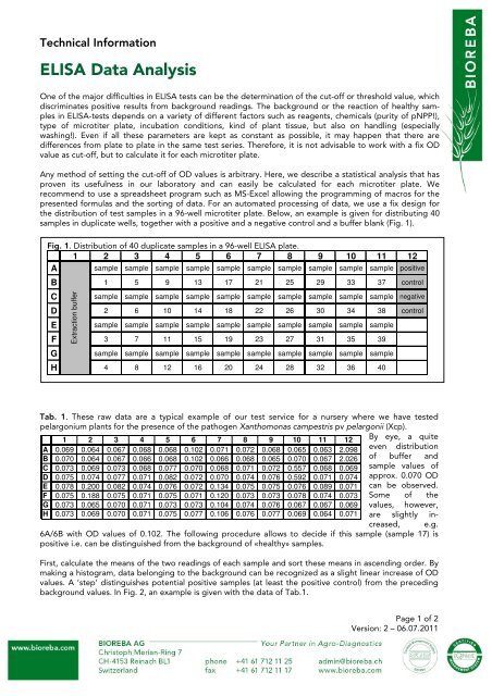
Tab. 1. These raw data are a typical example of our test service for a nursery where we have tested
pelargonium plants for the presence of the pathogen Xanthomonas campestris pv pelargonii (Xcp).
1 2 3 4 5 6 7 8 9 10 11 12
A 0.069 0.064 0.067 0.068 0.068 0.102 0.071 0.072 0.068 0.065 0.063 2.098
B 0.070 0.064 0.067 0.066 0.068 0.102 0.066 0.068 0.065 0.070 0.067 2.026
C 0.073 0.069 0.073 0.068 0.077 0.070 0.068 0.071 0.072 0.557 0.068 0.069
D 0.075 0.074 0.077 0.071 0.082 0.072 0.070 0.074 0.076 0.592 0.071 0.074
E 0.078 0.200 0.082 0.074 0.076 0.072 0.134 0.075 0.075 0.076 0.089 0.071
F 0.075 0.188 0.075 0.071 0.075 0.071 0.120 0.073 0.073 0.078 0.074 0.073
G 0.073 0.065 0.070 0.071 0.073 0.073 0.104 0.074 0.076 0.067 0.067 0.069
H 0.073 0.069 0.070 0.071 0.075 0.077 0.106 0.076 0.077 0.069 0.064 0.071
By eye, a quite
even distribution
of buffer and
sample values of
approx. 0.070 OD
can be observed.
Some of the
values, however,
are slightly increased,
e.g.
6A/6B with OD values of 0.102. The following procedure allows to decide if this sample (sample 17) is
positive i.e. can be distinguished from the background of «healthy» samples.
First, calculate the means of the two readings of each sample and sort these means in ascending order. By
making a histogram, data belonging to the background can be recognized as a slight linear increase of OD
values. A ‘step’ distinguishes potential positive samples (at least the positive control) from the preceding
background values. In Fig. 2, an example is given with the data of Tab.1.
Page 1 of 2
Version: 2 – 06.07.2011

Fig. 2. Histogram of sorted mean values.
Tab. 2. Formula for calculation of the cut-off value
cut-off = mean + 3 s + 10 %
In this histogram, means 1 - 35 show a linear
increase of OD values. The 36 th value exhibits a
clear increment compared to the foregoing
values. This «step» has to be determined for
each processed microtiter plate. The calculation
of the cut-off then indicates if the next values
on the right side of the step (indicated with an
arrow) can be considered as positive or not; in
other words, if these values are significantly
different from the preceding «background». In
this example, the calculation of the cut-off has
been done with mean values 1-35 using the
following formula (Tab. 2):
mean: mean of the mean values up to the step (mean values 1-35) = 0.072
s: standard deviation of first 35 mean values = 0.004
cut-off = (0.072 + (3 x 0.004)) x 1.1 = 0.092
Tab. 3. Calculation of means and comparison with cut-off value (values in mOD)
1 2 3 4 5 6 7 8 9 10 11 12
mean 73 64 67 67 68 102 69 70 67 68 65 2062
A 64 67 68 68 102 71 72 68 65 63 2098
B 64 67 66 68 102 66 68 65 70 67 2026
result - - - - positive - - - - - positive
mean 72 75 70 80 71 69 73 74 575 70 72
C 69 73 68 77 70 68 71 72 557 68 69
D 74 77 71 82 72 70 74 76 592 71 74
result - - - - - - - - positive - -
mean 194 79 73 76 72 127 74 74 77 82 72
E 200 82 74 76 72 134 75 75 76 89 71
F 188 75 71 75 71 120 73 73 78 74 73
result positive - - - - positive - - - - -
mean 67 70 71 74 75 105 75 77 68 66 70
G 65 70 71 73 73 104 74 76 67 67 69
H 69 70 71 75 77 106 76 77 69 64 71
result - - - - - positive - - - - -
In Tab. 3, all means
were compared with
the cut-off value of
92 mOD. The means
of the samples
3 (194 mOD),
17 (102 mOD),
23 (127 mOD),
24 (105 mOD), and
34 (575 mOD)
were interpreted as
positive. To avoid
false positives, check
the single values as
well. In some cases,
one value can be
relatively high (e.g.
caused by insufficient washing) and therefore giving a mean that corresponds not to the reality. Therefore,
as a rule, check if both values contributing to the calculation of the mean are above the cut-off.
Recommendation: The level of background can be different for different plant tissues (e.g. leaves, sprouts,
and tubers) or for different species/varieties of plants. In order to obtain an even distribution of the unspecific
reactions contributing to the background, use as homogenous samples as possible in one microtiter
plate.
Conclusion: This data interpretation helps to avoid false negatives in case of weak positive samples with an
antigen concentration near the detection limit. It allows therefore taking full advantage of the sensitivity of
ELISA tests.
Page 2 of 2
Version: 2 – 06.07.2011