Conceptual Design for a Gamma-Ray Large Area - SLAC - Stanford ...

Conceptual Design for a Gamma-Ray Large Area
Space Telescrope (GLAST) Tower Structure
Daniel Alex Luebke
Stanford Linear Accelerator Center
Stanford University
Stanford, CA 94309
SLAC-Report-489
August 1996
Prepared for the Department of Energy
under contract number DE-AC03-76SF00515
SLAC-R-489
Printed in the United States of America. Available from the National Technical Information
Service, U.S. Department of Commerce, 5285 Port Royal Road, Springfield, VA 22161.

CONCEPTUAL DESIGN FOR A GAMMA-RAY LARGE AREA
SPACE TELESCOPE (GLAST) TOWER STRUCTURE
A THESIS
SUBMITTED TO THE DEPARTMENT OF AERONAUTICS AND
ASTRONAUTICS
AND THE COMMITTEE ON GRADUATE STUDIES
OF STAN-FORD UNIVERSITY
IN PARTIAL FULFILLMENT OF THE REQUIREMENTS
FOR THE DEGREE OF
ENGINEER
BY
Daniel Alex Luebke
August 1996

I certify that I have read this thesis and that in my opinion
it is fully adequate, in scope and in quality, as a thesis for
the degree of Engineer.
Robert Twiggs
(Academic Advisor)
Elliott Bloom
(Research Advisor)
Stephen Tsai
(Principal Advisor)
Approved for the University Committee on Graduate
Studies:
. . .
111

Abstract
The main objective of this work was to develop a conceptual design and
engineering prototype for the Garnma-ray Large Area Space Telescope (GLAST) tower
structure. This thesis describes the conceptual design of a GLAST tower and the
fabrication and testing of a prototype tower tray.
The requirements were that the structure had to support GLAST’s delicate silicon
strip detector array through ground handling, launch and in orbit operations as well as
provide for thermal and electrical pathways. From the desired function and the given
launch vehicle for the spacecraft that carries the GLAST detector, an efficient structure was
designed which met the requirements.
This thesis developed in three stages: design, fabrication, and testing. During the
first stage, a general set of specifications was used to develop the initial design, which was
then analyzed and shown to meet or exceed the requirements. The second stage called for
the fabrication of prototypes to prove manufacturability and gauge cost and time estimates
for the total project. The last step called for testing the prototypes to show that they
performed as the analysis had shown and prove that the design met the requirements.
As a spacecraft engineering exercise, this project required formulating a solution
based on engineering judgment, analyzing the solution using advanced engineering
techniques, then proving the validity of the design and analysis by the manufacturing and
testing of prototypes. The design described here met all the requirements set out by the
needs of the experiment and operating concerns. This strawman design is not intended to
be the complete or final design for the GLAST instrument structure, but instead examines
iv

some of the main challenges involved and demonstrates that there are solutions to them.
The purpose of these tests was to prove that there are solutions to the basic mechanical,
electrical and thermal problems presented with the GLAST project.
,
V

Acknowledgments
There are many people and agencies who made this work possible. This long list is
only a partial list of the most notable contributors.
I’d like to thank my advisors, Elliott Bloom, Stephen Tsai; and Bob Twiggs;
Stanford Linear Accelerator Center’s (SLAC) Terry Anderson, Bill Atwood, Joe Ballam,
John Broeder, Lynn Cominsky, Linda Lee Evans, Bruce Feerick, Gary Godfrey, John
Hanson, Chad Jennings, Y.C. Lin, Peter Michaleson, and Pat Nolan; Stanford Satellite
Systems Development Lab’s (SSDL) Raj Batra, Jeff Chan, and Alison Nordt; Stanford
Structures And Composites Lab’s (SACL) Sung Ahn, Tracy Colwell, Steve Huybrechts,
George Springer and Qiuling Wang; Lockheed-Martin’s Dave Chenette, Eric Herzberg,
George Nakano, and Jeff Tobin; Space Systems Loral’s Steve Berglund, and Fred
Wooley; The National Aeronautics and Space Administration’s (NASA Ames) Roger Arno,
and Gary Langford; Stanford Center for Integrated Syatems (CIS) Nanofabrication Lab’s
Nancy Latta, Mary Martinez , and Bob Wheeler; Aptos Corporation’s Scott Grahm;
Promex Corporation’s Bill Stansbury, and Glen Stansbury; DynaFlex Corporation’s Scott
Russel; Merlin Technologies’ Walt Wilson; The International Center for Theoretical
Phsyics’ (ICTP) Andreas Cicuttin, Albert0 Colavita, and Fabio Fratnik; The Italian Center
for Nuclear Physics’ (INFN) Guido Barbullini; San Francisco State’s Abraham
Anapolsky, and Barbara Neuhauser; University of Santa Cruz’s Robert Johnson;
University of Chicago’s Renee Ohn, and Mark Oreglia; University of Tokyo’s Tune
Kamae; The Navel Reasearch Lab’s (NRL) Neil Johnson, Michael Lovellett, and Kent
Wood; The Department Of Energy (DOE); Bryte Technologies; Stanford University’s
Department of Aeronautics and Astronautics, Department of Physics and Department of
Mechanical Engineering; and all other businesses and associates who helped on this project
and to all my friends at Stanford and around the world.
vi

Most importantly my thanks to Brad “swing jumper” Betts, Rick “danger seeker”
Lu, James “the man” Myatt, my Mom, Dad, sister Aviva and Debbie for their help and
support.
I
Vii

List of Symbols
a
ag
4,
a
C
IflUX
D
6
6 max
&
&SSD
Et
E
g
Gs
h core
I
H
Albedo (30% of direct solar, 407 W/m’)*
Acceleration in gravities
Radiator area for spacecraft (m*)
Solar absorptivity (0.15 for radiators, 0.01 for thermal blankets)
Maximum distance f?om neutral axis
Flexural stifness modulus matrix
Deflection (meters)
Maximum deflection (meters)
Mechanical strain = o/E
Constant strain component
Strain in silicon strip detector
Solar Emissivity (0.8 for radiators, 0.01 for thermal blankets)
Modulus of elasticity (pa)
Gravity of acceleration (9.8 m/s*)
Solar constant (1358 W/m*)
Thickness of composite core (meters)
Area moment of inertia (meters4)
Altitude of orbit (600 km)
l MKS units used except when English units are given as standard for manufacturing
‘Viii

k
K mn
K trayn
L
L trak
M ma.x
Gd
h0k
PO
Q
P
Pe
41
R,
CT
0 max
0,
hSD
tf,ce
X
Y
z
Thermal conductivity (W cm-’ K’)
0.664+0.52 1 p,-0.203p,, a factor which accounts for the reflection of collimated
incoming solar energy off a spherical Earth.
Fourier coefficients
Curvature of tray
Length of side of tray
Length of the tracker section (meters)
Maximum moment (N m)
Mass of calorimeter section (N m)
Mass of tracker section (N m)
Distributed Load (Pa)
Composite stifness matrix
Mass denisity (kg/cm3)
Angular radius of Earth (RJ(H + k))
Earth IR emission (237 W/m2)
Radius of Earth (6378 km)
Mechanical stress (Pa)
Maximum mechanical stress
Stefan-Boltzmann constant (5.67E-8 W m.-2K-4)
Thickness of silicon strip detector (m)
Thickness of composite facesheet (meters)
X silicon layer, bottom layer of detectors on tray
Y silicon layer, top layer of detectors on tray
Elemental number on periodic chart (radiation length)
ix

List of Acronyms
CSI . . . . . . . . . . . . . . . . . . Cesium Iodide crystals, used in calorimeter
CTE . . . . . . . . . . . . . . . . Coefficient of Thermal Expansion, describes amount materials expand
when exposed to temperature gradients
CTT . . . . . . . . . . . . . . . . Conductive Transfer Tape, double sided tape which offers high thermal
conductivity
CVCM . . . . . . . . . . ..Collectable Volatile Condensable Materials, percentage of evaporated
material that is condensable
EOL . . . . . . . . . . . . . . . . End Of Life, design condition exemplifying changes in materials over time
ESD . . . . . . . . . . . . . . . . Electrostatic Discharge, the transfer of potential static electricity by an
electrical spark
FEM . . . . . . . . . . . . . . . Finite Element Model, engineering computer tool to analyze physical
systems
GEVS . . . . . . . . . . . . . . General Environmental Vehicular Specifications, report put out by NASA
which lists basic requirements for spacecraft
X

GLAST . . . . . . . . . . . Gamma-ray Large Area Space Telescope
IDL . . . . . . . . . ,. . . . . ..Interactive Design Language
IR . . . . . . . . . . . . . . . . . . . . Infrared, energy range exemplified by heat emittance
ML1 . . . . . . . . . . . . . . . . Multilayer Insulation, thermal insulation blankets
NASA . . . . . . . . . . . ..National Aeronautics and Space Administration, the principal space
agency responsible for defining spacecraft requirements
RVC . . . . . . . . . . . . . . . . Reticulated Vitreous Carbon, expanded carbon foam structural spacer
material
SSD . . . . . . . . . . . . . . . . . Silicon Strip Detector, device for measuring the passage of charged
particals en-mass
SSM . . . . . . . . . . . . . . . . Second Surface Mirror, device used to radiate heat energy
TAB . . . . . . . . . . . . . . . Tape Automated Bonding system for providing electrical connections
TML . . . . . . . . . . . . . . . Total Mass Loss, percentage of mass lost due to evaporation
W . . . . . . . . . . . . . . . . . . Ultra Violet, range of electromagnetic energy emission
xi

Contents
1 Introduction 1
Statement of Problem .............................................................................. I
Design Concept Summary ..................................................................... 3
The Space Environment ........................................................................ 4
Contributions of Dissertation ..................................................................... 5
2 : Tower Design Issues 6
Tower Design ...................................................................................... 6
Layup of SSDs on Tray ........................................................................... 7
Tray Mounting .................................................................................. 7
SSD Mounting .................................................................................. 9
Electrical Connections ........................................................................ 10
Calorimeter and Tower Wall Design ........................................................... II
Instrument Strong-back Design ................................................................ II
Satellite Bus Design ............................................................................. 12
3 : Design Specifications 14
Material Audit .................................................................................... 14
Attitude and Thermal Control ................................................................... 15
Orbit, Size, and Weight ......................................................................... 15
Expected Loads .................................................................................. 15
Operating temperatures .......................................................................... 16
4 : Thermal, Material, and Electrical Considerations 17
Thermal Considerations to meet Specifications .............................................. 17
Thermal Conditions ........................................................................... 17
Thermal Subsystem ........................................................................... 18
Thermal Contact Resistance and Heat Pipes .............................................. 20
xii

Spacecrafr Materials to meet Specifications. .................................................. 21
Composites ....................................................................................
Metals ..........................................................................................
I
22
24
Adhesives ...................................................................................... 24
Other materials ................................................................................ 25
Electrostatic Discharge .......................................................................... 25
5 : Analysis of Design
27
Finite Element MO&~ ............................................................................ 27
Structural Analysis: Strength and Deflection ................................................. 28
SSD Tray ...................................................................................... 28
Tower ..........................................................................................
30
Grid ............................................................................................. 32
Vibrational Analysis: Natural Frequency Estimutes .......................................... 34
SSD Tray ...................................................................................... 34
Tower Structure ............................................................................... 36
Grid Structure ................................................................................. 37
Themzal Analysis, Operating Temperature Estimates ........................................ 38
SSD Tray ...................................................................................... 38
Tower Wall .................................................................................... 39
Grid. ............................................................................................ 41
On Orbit Temperatures ..........................................................................
6 : Fabrication of Prototypes 47
Space Qualification .............................................................................. 47
Built in Testing Schemes ........................................................................ 47
Back-plane continuity check ................................................................. 47
Back-plane design ............................................................................ 48
Dummy detector ............................................................................... 50
Manufacturing of a Tray ........................................................................ 51
Manufacturing processes ..................................................................... 51
7 : Testing of Prototypes
53
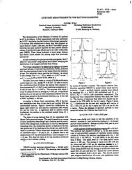
Random Vibration Tests ........................................................................ 53
Vibration Equipment Setup .................................................................. 53
Shake Test ..................................................................................... 54
Thermal Cycling under Vacuum ............................................................... 55
Thermal Equipment Setup ................................................................... 55
Thermal/vacuum Tests ....................................................................... 55
xlll
.a.
43

8 : Final Results 57
Post test ........................................................................................... 57
Mass Estimates ................................................................................... A 58
Physics Per$ormance Numbers ................................................................ 60
Concluding Remarks ............................................................................ 60
BIBLIOGRAPHY ............................................................................... 61
APPENDIX A - ANSYS STATIC DEFLECTION AND FREQUENCY GRID CODE 62
APPENDIX B - ANSYS TRAY CODES ..................................................... 68
APPENDIX C - ANSYS TOWER CODES .................................................. 72
APPENDIXD-ANSYSTHERMALANDRADIATIONGRIDCODES.. ............. 78
APPENDIX E - MATLAB THERMAL CODE FOR WALL ............................... 84
APPENDIX F - ANSYS THERMAL WALL FEM ......................................... 88
APPENDIXG-lDLCODEFORONORBlTTEMPERATURES.. ..................... 92
Xiv

List of Figures
Figure l-l - Artists concept of GLAST (showing tracker and calorimeter) ................... .2
Figure l-2 - Layout of towers ....................................................................... 3
Figure 2-l - Lay-up of tray (exploded view) ...................................................... 8
Figure 2-2- Electrical connection of Silicon Strip Detectors (SSDs) ............................ 9
Figure 2-3 - Structural grid design ................................................................ 12
Figure 2-4 - Schematic of GLAST ................................................................ 13
Figure 4-l - Composite core laminate ............................................................ 23
Figure 5-l - FEM stress analysis of structural grid ............................................. 33
Figure 5-2 - FEM modal analysis of structural tray ............................................. 35
Figure 5-3 - FEM modal analysis of tower ...................................................... 36
Figure 5-4 - FEM modal analysis of structural grid ............................................ 37
Figure 5-5 - Temperature distribution down tower wall ....................................... 39
Figure 5-6 - FEM thermal analysis for temperature rise down tower wall ................. .40
Figure 5-7 - FEM thermal analysis for temperature distribution across grid ................ .42
Figure 5-8 - Maximum temperatures of GLAST radiator surface as function of rotations. 44
Figure 5-9- Maximum temperatures of GLAST radiator surface as function of rotations . . 45
Figure 6-l - Circuit design for electrical connection of back-plane ........................... 49
Figure 6-2 - Dummy detector testing scheme .................................................... 50
Figure 7-l - Response of center of tray under random vibration .............................. 54
Figure 7-2 - Sample thermal vacuum temperature cycle ........................................ 56
xv

List of Tables
Table 4- 1 - Spacecraft material properties ........................................................ 22
Table 8-l - Mass and radiation lengths in tray ................................................... 58
Table 8-2 - Mass estimates for GLAST .......................................................... 59
‘xvi

CHAPTER 1. INTRODUCTION
1 Introduction
Statement of Problem
The main objective of this work was to develop a conceptual design and engineering
prototype for the Gamma-ray Large Area Space Telescope (GLAST, Figure l-l) tower structure.
This thesis describes the conceptual design of a GLAST tower and the fabrication and testing of a
prototype tower tray.
The novelty of the GLAST instrument is that it is a high energy gamma-ray telescope based
on silicon strip detector (SSD) technology. This new technology provides an effective way to
measure the passage of charged particles while still allowing for a highly modular structure.
Because of the Earth ‘s atmosphere, only the highest energy gamma-rays are detectable by
ground based observatories. By using detectors in orbit, gamma-rays can be viewed before they
are absorbed by the atmosphere. The purpose of the GLAST instrument is to measure the
interaction of gamma-rays in the detector in order to determine their energy and direction. From
this information we might further understand the physics of gamma-ray emissions from
astrophysical sources such as relativistic jets emanating from active galactic nuclei, gamma-ray
bursts, pulsing neutron stars, and the diffuse galactic and extragalactic emission. The combination
of wide field of view, high angular resolution, good sensitivity, and a wide-energy bandwidth
make telescopes based on silicon strip technology well suited for the observation of such sites of
cosmic particle acceleration mttp://www-glast.stanford.edu].
The basic component of the GLAST instrument is a tower which is composed of a tracker
and a calorimeter (see Figure l-2). The tracker section is used to convert the incoming gammarays
to electrons and positrons and then track the paths of the subsequent electromagnetic shower
of these particles. The calorimeter is then used to measure all the remaining energy from the
electromagnetic shower and thus make an energy measurement of the gamma-rays. The work
presented here focuses on the design and prototyping of the tracker section of the GLAST tower -
1

CHAPTER 5. ANALYSIS OF DESIGN
specifically the mechanical support of the SSDs. Additionally, to provide accurate models for the
tray analysis, detailed designs were done for electrical connections and mechanical bonding of
detectors, as well as the main structural support for the instrument.
Figure 1 -I - Artists concept of GLAST (showing tracker and calorimeter),

CHAPTER 1. INTRODUCTION
Design Concept Summary I
The proposed GLAST instrument consists of a 7x7 array of towers, each with a stack of
silicon detectors (tracker section) followed by an array of Cesium Iodide (CsI) crystal detectors
(calorimeter section). These towers are supported on a mounting structure (grid) that sits above the
spacecraft bus (see Figure l-2).
In designing the GLAST structure, two critical design criteria for components were
identified -- modularity and accessibility. These criteria led to an identical design for each of the
towers, resulting in straightforward manufacturing, assembly, and disassembly of the instrument.
This design philosophy also extends into the tower itself, where each tracker tray is nearly
identical, as is each calorimeter detector. Although there are many benefits for this modular
structure, it introduces a difficulty in designing for robust thermal and mechanical connections.
Towers
Grid
Bus
Figure I-2 - Layout of towers
3
Tracker
Calorimeter

CHAPTER 1. INTRODUCTION
The trays in the tracker section required substantial engineering. The purpose of the trays
is to support the delicate SSDs through ground handling, launch and on orbit operations. The
requirement for the tower structures are high stiffness, good thermal pathways, and maximum
transparency to gamma-rays. This last requirement was a main driver in the tower designs,
requiring minimal material (in-line with the detectors) that might cause the gamma-rays to convert
to electrons and positrons before reaching the SSDs.
The solution was for the trays to utilize composites. The directional nature of composites
allowed the strength, stiffness, and thermal properties to be tailored to meet the requirements.
Additionally, by using a laminate consisting of a core spacer in-between thin layers of high
modulus composite fibers, high strength and stiffness was achievable using minimal material mass
and volume. Advanced composites also offer excellent thermal conductivities, rivaling the most
conductive metals.
The Space Environment
Because this instrument must operate in the harsh environment of outer space, the demands
of space must be understood and accounted for in the design. The most obvious characteristic of
space is the hard vacuum. The problem here is that many materials (resins, adhesives, liquid
lubricants and even some metals) evaporate (outgas) in a vacuum. Excessive outgassing can lead
to the degradation of material properties and can also affect other components. For example, since
there is no force to carry the outgassed particles away from the spacecraft, these particles remain in
a cloud around it or condense onto its colder surfaces. In this way, outgassing can degrade optical
surfaces, radiators and solar arrays, and even cause shorting of electrical circuits and promote
corona or electrical discharge Williamson, 1990, pg. 291. The high vacuum poses another
problem by severely reducing thermal conduction between components.
The temperature regime of space must also be accounted for, or serious problems can arise.
In orbit, the temperature range is much larger than normally experienced on Earth and, without air
for convective cooling, the differentials can be extreme. These extremes in temperature cause
many problems. Thermal cycling can produce fatigue, fracture and de-bonding through differential
expansion and contraction. In addition, low temperature promotes condensation while high
temperature increases outgassing. While this can pose serious problems for some components, the
main structure is generally not exposed to these extreme temperatures because the spacecraft core
temperature is controlled to protect the payload and subsystem equipment.
‘4

CHAPTER 1. INTRODUCTION
Radiation such as x-rays, gamma rays, alpha particles, protons, and electrons can affect
many systems on a spacecraft, including the structural subsystem. Ultra violet (UV) radiation can
degrade polymeric materials while x- and gamma radiation can scatter electrons in metals. This
scattering of electrons may eventually decrease electrical conductivity, a particularly undesirable
effect in materials which transmit low signal currents Williamson, 1990, pg. 3 11.
In space, physical properties of material may also degrade over time. It is therefore critical
for all calculations to be designed with end of life (EOL) properties in mind. This is particularly
true when calculating solar cell efficiencies, radiator efficiencies, thermal surface properties and
heat generation in electronics.
However, there are some advantages of the space environment. There is no corrosion and
space offers inherently good electrical insulation, meaning that high voltage electrical components
can be positioned closer together before arcing problems occur Williamson, 1990, pg. 3 11.
Contributions of Dissertation
In summary, there are several factors which must be considered in designing the GLAST
instrument tower. The tower structure must be designed to support all the tower components while
not interfering with the experiments. It must be versatile and allow for easy assembly,
disassembly and modifications. Because of the large size of the instrument and the tight tolerances
between components, special production techniques must be accounted for in the designs. All this
must be accomplished with minimal cost and time constraints.
This thesis offers a basic concept for designing and manufacturing the GLAST instrument
structure and defines some of the specifications that will be needed to for the final design. While
the solutions offered in this thesis do not necessarily provide the best designs, they have
demonstrated the feasibility of the GLAST tower system.

CHAPTER 2. TOWER DESIGN ISSUES
2 : Tower Design Issues
In this chapter, many issues for the GLAST instrument are examined, including SSD
mounting and electrical connections, designs for the tracker, calorimeter, tower wall, structural
strong-back, and satellite bus. While not all aspects or issues of the instrument are explored, the
main issues are addressed sufficiently well to obtain a “big” picture of the system.
Tower Design
The basic configuration of the GLAST instrument is based on five design criteria:
performance, cost, ease of manufacturing, ease of assembly (serviceability), and versatility of
design. Trade studies were performed using the above design parameters to address two critical
design issues: the method for holding the trays in the tracker section, and configuration of the
tower walls.
The first set of trade studies assessed two designs for the mounting of trays. The
competing designs were for the “rack” and the “stack” tower designs where trays are either slid
into place like shelves or stacked on top of one another, respectively. Because of thermal contact
and ease of assembly reasons, the rack design was chosen.
The second trade study was performed to deterrnine the most suitable configuration for the
tower walls. The tower walls must provide structural support for trays, thermal pathways for heat
dissipation, and space for electrical cables. They must do all this with minimum interference to
the gamma-rays products being measured. The three basic configurations for the tower walls had
to do with me number of walls. A two walled tower had the lowest material audit and was
sufficient for thermal needs but mechanically weak. While three walls improved the mechanical
properties, for robustness, the design selected as the baseline was with four walls. Although this
design resulted in an increased material audit for the tower, this effect was offset by the selection of
higher performance materials (higher strength, stiffness and radiation length).
6

CHAPTER 2. TOWER DESIGN ISSUES
Layup of SSDs on Tray
SSD layup and corresponding electrical connections drive the mechanical requirements for
the structural tray. The tray must be stiff and strong enough to protect the detectors and electrical
connections when loaded.
Tray Mounting
A honeycomb composite tray provided the required properties of strength and stiffness to
protect the SSDs and wirebonds. The need to mechanically attach and thermally couple the tray to
the walls still remained. A simple solution was to add a “close-out” around the tray (see Figure 2-
1). The close-out provided secure mounting points for bolts and also provided enough material
and surface area to transfer heat to the tower walls. The relatively large amount of concentrated
material in the close-out, however, required a good low Z, thermally conductive material. Because
GLAST will have a 2n field of view, gamma-rays can penetrate tower walls before registering on
the SSDs. Also, because the walls offer the only thermal path from the readout electronics to the
satellite bus, the walls will have to be good conductors of heat. The challenge is to find a suitable
low Z, thermally conductive material (e.g., Be, composites; See Chapter 4).
The “active” area is defined as the atea of the SSD minus a small inactive border on the
edges of the detectors. All other area within the instrument is classified as “dead” area, because it
cannot register particle tracks. The efficiency of the GLAST instrument increases proportionally to
the active area of the SSDs. In order to minimize dead area, clearances between components in the
tower and clearances between towers must be kept to a minimum. To reduce dead area created by
the readout electronics, the SSDs will be daisy chain bonded together, requiring only one set of
readout electronics per four detectors.
The readout electronics (pre-amplifier, shaper, filter, etc.) are 2 mm wide silicon devices
that he on the periphery of two sides of a tray. These electronics are the main source of the heat
generated in GLAST and thus drive me thermal design. To reduce problems resulting from heat
generation and dead area, these devices have been designed to be as small and efficient as possible.

CHAPTER 2. TOWER DESIGN ISSUES
Figure 2-1 - Lay-up of tray (exploded view)
The area in the tower includes four 2 mm walls, 3.5 mm on two edges for electronics and
electrical connection, and 416 I.L~ between all components. This design gives exactly the
equivalent of 43 dead strips between active area in adjacent towers. In the current design, with a
736 p dead band around the periphery of each detector, the dead area in the instrument is 11%.
The design of the tracker section, as discussed earlier, is a vertical array of 12 horizontal
trays, spaced apart by 3 cm and held together by four walls. These walls offer structural support
in addition to thermal and electrical pathways. Each horizontal tray in the tracker section holds 32
SSDs. Each SSD is a 6x6 cm square pieces of 500 pm thick, high resistivity silicon with 249
parallel strip implants nearly 6 cm in length and 236 km apart (see Figure 2-2).
8

CHAPTER 2. TOWER DESIGN ISSUES
Readout
electronics
SSD
Electrical
connection
I..... . . . . . . . .I.. .
4
249
strips/SSD
I’ I’ I’ I- 1.1.1.. Ic . . . . . . . .
Figure 2-2- Electrical connection of Silicon Strip Detectors (SSDs)
SSD Mounting
+6crn4;
I I
Another trade study was done for establishing the specific method for configuring the
SSDs on the each tray. As the SSDs have been selected to be single sided (for reasons of cost,
versatility and ease of handling), two complete layers are required to determine X and Y
coordinates for an incoming gamma-ray. One important design factor is that these layers be as
close together as possible (directly on top of each other) to insure a good coordinate value for three
dimensional tracking.
There are two basic concepts for mounting the two SSD layers. The first is to produce two
trays each with 16 detectors mounted upward. Tray pairs would be mounted facing each other in
close proximity with one tray oriented 90 degrees from the other. This allows each tray to be
manufactured separately, reducing the cost risk by 50% should a tray get damaged. Such a design
leads to easier manufacturing, but will likely compromise the angular resolution of the instrument.
Because of the gap that must exist between trays (primarily for vibrational clearances) in this
design, the X and Y coordinates are not located at the same Z position. This complicates data
analysis and reduces angular tracking resolution. The distance between detectors is a function of
mounting techniques. The challenge is to find a scheme that will reduce the gap between layers to
an acceptable value while still being straightforward to mount in the tower.
The second concept for mounting the two SSD layers is to mount the Y layer directly on
top of the X layer. This design offers the minimum distance between layers giving the maximum
9

CHAPTER 2. TOWER DESIGN ISSUES
accuracy for the instrument. In this scheme, the mounting of a layer in the tower is very
straightforward since it is only a single tray. However, extreme care must be taken in mounting
the Y layer, as damage could be incurred on the working X layer below. If something goes
wrong with a tray, a total of 32 detectors would potentially have to be scrapped, compared to only
16 detectors in the other design. Also, repair of the covered X layer becomes virtually impossible.
As a baseline, this single tray design was selected.
Electrical Connections
Regardless of which concept for mounting is used, the challenge is still the making of the
4000 electrical connections per layer of SSDs. Each layer of 16 detectors is electrically bonded
together in four strips of four (each strip acting as a single, long, SSD with 249 channels) with the
output of each channel going to a low power preamplifier. Searching for solutions to the mass
bonding problem led the GLAST collaboration to study such familiar techniques as Tape
Automated Bonding (TAB) and Bump bonding, and to develop a combination of these two
techniques that was named flex bonding. The process called for making small flexible circuits
(similar to TAB circuits) which are ultrasonically welded to small Gold bumps on adjacent
detectors connecting the channels. This process resulted in many excellent characteristics including
high strength and allowed’ for rapid mass bonding with the flexibility of modifications and remanufacturability,
More testing will be required to qualify this process for the GLAST instrument.
One idea, still in the conceptual stage, uses an electrically conductive thermoplastic Z-axis adhesive
film (such as 3M’s 530313). Rather than using the complex ultrasonic welding to bond the mass
electrical connections, this process reduces the complexity and cost of these electrical connections.
After assessing the various methods, wirebonding was selected for electrically connecting
detectors because it is well known, well used in industry, cost effective and meets all of the
requirements. During this process, a thin (-1 mil) Aluminum wire is ultrasonically welded to form
an electrical path between two detectors. There are some trade-offs with wirebonds. They are less
mechanically robust than flex (6-8 grams pull strength vs. 40-60 grams) and they must sit above
the components that they are connecting, increasing the vertical distance between X and Y detector
planes (reducing the angular resolution when tracking). The limit to which wirebonds can be
“flattened” needs to be explored. Regardless, wirebonds meet the requirement of this project.
10

CHAPTER 2. TOWER DESIGN ISSUES
Calorimeter and Tower Wall Design
At the base of each tower is a Cesium Iodide (CsI) calorimeter. Each calorimeter consists
of an 8x8 pack of CsI crystals, each measuring 3x3~19 cm. The crystals are decoupled optically
from each other (wrapped in an opaque material such as Teflon or Tyvex) with a photodiode and
preamplifiers on both ends of each crystal. The power required for the 128 photodiodes and their
readouts can be as much as 5 watts. The purpose of the CsI is to convert the deposited shower
energy into light. The photodiodes give an electrical signal proportional to the amount of light and
hence the energy of the gamma-ray.
Because the calorimeter sits directly beneath the tracker section, the tower walls that hold
the trays simply extend to support the calorimeter as well. The tower walls are 60 cm in length and
2 mm thick.
Instrument Strong-back Design
In order to provide a scheme for attachment of the GLAST instrument to the spacecraft and
to provide boundary conditions for analysis of tower performance, a structural strong-back had to
be designed. The solution, after many iterations, came in the form of a structural grid that spanned
the whole area under the towers. The grid also doubled as a heat conduction path from the towers
to the thermal radiators on the exterior of the spacecraft. The grid is a simple, efficient design that
is relatively easy to manufacture (even out of composites), inherently stiff and strong, and is
straight-forward to analyze. The configuration that was selected was a 7x7 grid of squares, each
the size of a tower (see Figure 2-4), the idea being that each tower simply bolts around the lip of
each grid, providing ample surface area for support and thermal contact. The thickness and height
of the ribs are determined by considering the requirements for stiffness and thermal conductivity.
11
,

CHAPTER 2. TOWER DESIGN ISSUES
Figure 2-3 - Structural grid design
Satellite Bus Design
As long as the instrument is self-supportive, the design of the bus is not critical for the
design of the instrument. When doing analyses, certain assumptions must be made for how load
paths run from the instrument to the satellite bus and for the amount of heat generated by the bus.
A simple design for an instrument/bus layout is shown in Figure 24. This design alleviates the
need for the bus structure to hold the instrument. Instead, the instrument structure itself holds the
bus where the components of the bus are hung onto the underside and periphery of the structural
grid, making electrical connections through the grid. Thermally, the bus components conduct their
heat directly to the radiators, and not through the grid. Thus, the thermal analysis for the grid does
not account for heat generated by the bus. The structural analysis, however, requires the
knowledge of how the structural grid is supported. While not necessarily the final bus design for
GLAST, this bus design supplies the necessary compatibility information to analyze the
instrument.
-12
m

CHAPTER 2. TOWER DESIGN ISSUES
. I. r . 1.1.
Spacecraft -m
radiators
I
Solar array
Figure 2-4 - Schematic of GUST
. ..-
. ..#......-~-~--.......~~
--....
..-
..**
,.-- Field of View ‘-‘--q..
,- --. ,
.’
9. .
-.
‘I
‘.
Multilayer insulation
‘. thermal blanket
Rocket ring
13
Tracker
. . . . . . . . . . . 1 . . . . . . . . . I. I.
Calorimeter
Solar array
Spacecraft electronics

CHAPTER 3. DESIGN SPECIFICATIONS
3 : Design Specifications
In the previous chapter the major design issues were presented and discussed in detail,
providing an in depth look at the “big picture” of the GLAST design. In this chapter, the
specifications are defined which will be used to analyze and qualify designs in Chapter 5.
Specifically, this chapter covers the specifications for material audit, instrument weight, expected
loads, and allowable temperatures.
Material Audit
The design criteria for GLAST require that the tower structure minimally absorb or produce
the photons which GLAST detects. The materials considered for the tower structure all have
different radiation lengths.’ As an example, the radiation length of Lead is 0.56 cm while that of
Beryllium is 35.3 cm.
To cause a gamma-ray to convert to an electron-positron pair, a layer of converter material
(280 pm, or 5% of a radiation length of Lead) is placed directly over each tray. The material used
for supporting the detectors should be much less than the converter layer, preferably under 1% of a
radiation length. Additional material in the supports generates background processes that degrade
the performance of the instrument.
To obtain a more uniform acceptance for the instrument, the supporting materials must be
spread out over the detector area rather than having it concentrated in small regions. This
requirement is used to specify the material of the core spacer for the tray.
’ The mean distance over which a high energy electron loses all but l/e of its energy by bremsstrahlung.

_
CHAPTER 3. DESIGN SPECIFICATIONS
Attitude and Thermal Control ,
In order to have GLAST point toward specific gamma-ray sources in outer space, an active
control system must be implemented. A standard three axis control system was selected, where
momentum wheels are used for control and torquer coils are used to bleed off excess, built up
angular momentum.
To reduce complexity and cost, a passive control system for temperatures was selected.
Passive thermal control requires no energy, instead using only the thermal properties of various
materials to reach the desired temperatures. Heat is transported around the satellite, by passive
means, to radiators that, when pointed to objects of a lower temperature (like space), radiate the
heat away from the satellite. The fact that GLAST will be three axis stabilized opens the possibility
of active pointing of thermal control surfaces for better control of the spacecraft’s operating
temperature.
Orbit, Size, and Weight
The GLAST project is planned to be a “medium sized” NASA space mission. As a
baseline, the McDonnell Douglas Delta II 7920 launch vehicle was selected to provide design
specifications. For the given dimensions and weight to altitude limits of the Delta II, a Low Earth
Orbit (LEO - 600 km , 28.7” inclination - allows for 4500 kg) was selected as the design orbit.
The Delta II fairing limits the size of the satellite to a 100 inch diameter circle. The Delta II
baseline also defined the vibration and acceleration loading during launch to orbit.
Expected Loads
The characteristics of the Delta II launch vehicle defined the structural loads for the GLAST
instrument. The loads consist of steady state (axial and lateral) accelerations, acoustic vibrations,
shock, and sinusoidal and random vibrations. Acoustic and shock loads are difficult to analyze
and were not considered. Acceleration loads were applied to test the steady state stresses and
deflections of various components. Sinusoidal and random excitations were superimposed on
steady state accelerations to obtain composite accelerations for the dynamic structural design.
15

CHAPTER 3. DESIGN SPECIFICATIONS
Specifically, for a 4500 kg instrument, the Delta II produced a 6.0 g steady state acceleration and
an expected 8.7 gRMS random vibration load VASA GEVS, 1990, D-7,10]. ,
The launch excitation of a spacecraft is a function of the spacecraft mass and dynamic
characteristics, as well as the launch vehicle characteristics. To avoid dynamic coupling between
low frequency vehicle and spacecraft modes, the stiffness of the spacecraft structure must be
designed to produce fundamental frequencies above 35 Hz along the thrust axis and 15 Hz along
the lateral axes for “spacecraft hard-mounted at the spacecraft separation plane” [Delta II
Commercial Spacecraft Users Manual, 1987, 3-221. To verify the robustness of designs,
qualification testing for vibrations are completed (see Chapter 7). The qualification test assures that
the spacecraft, even with minor weight and design variations, can withstand the most severe
dynamic and environmental loads.
Operating temperatures
The temperature of the satellite varies widely both internally and around its exterior.
Temperature characteristics depend on solar illumination, internal heat generation and the details of
the thermal design itself. As a reasonable guide, the interior of the satellite should operate around
room temperature (0 “C is the preferred temperature). For a typical spacecraft, temperatures
usually range between -20 and +35 “C Williamson, 1990, pg. 1391.
The front end electronics and the SSDs themselves drive the thermal requirements. Both of
these components generate noise as they heat up. For the noise requirement, a maximum
temperature of +25 “C was selected as the design constraint. As electronics operate well at lower
temperatures, a lower limit of -25 “C was sufficient, resulting in the final thermal design
specification of 225 “C or lower.
16

CHAPTER 4. THERMAL, MATERIAL, AND ELECTRICAL
CONSIDERATIONS
4 : Thermal, Material, and Electrical
Considerations
Now that the specifications have been laid out, the technological considerations need to be
examined. In this chapter the thermal, material, and electrical considerations to meet the
specifications are reviewed.
Thermal Considerations to meet Specifications
Because of the demanding thermal requirements in orbit, special attention must be given to
the thermal subsystem. In the following section, the thermal conditions of space are discussed in
detail, along with the intricacies of the thermal subsystem including contact resistances and heat
pipes.
Thermal Conditions
Because GLAST will need to control its internal temperature within relatively tight
tolerances, the thermal control system is a critical aspect in the design. The heat input from the Sun
is 1358 W me2. In addition to the direct solar radiation heat input, there is heat input from reflected
energy off the Earth (for LEO satellites only ). The amount of incident solar radiation returned to
space by planetary albedo (solar reflection) is 407 W me2 and the input from the Earth itself from
infrared thermal radiation approaches 237 W mm2 [Hertz and Larson, 4241.
The temperature inside the spacecraft also depends on the amount of heat generated
internally. This is a function of the efficiency of all the electronic components. The expected heat
dissipated by the instrument is 645 watts (350 w from preamplifiers, 245 w from the calorimeters
17

CHAPTER 4. THERMAL, MATERIAL, AND ELECTRICAL
CONSIDERATIONS
and 50 w from miscellaneous electronics). The spacecraft bus has been allotted 350 watts, giving
a total baseline power consumption of 1 kW (EOL). This amount of heat generation drives the
sizing of thermal pathways and radiative surfaces. If this value changes, simple re-sizing of
radiator surfaces should compensate.
Because the GLAST instrument generates a substantial amount of heat internally, it is
expected to be a “hot” satellite. To control the heat exchange with the environment, sunlit areas of
the satellite should be covered by a thermal barrier while dark space pointing radiators should be
used to dump thermal energy.
A very simple equation to describe the radiation and absorption of thermal energy is:
where a is the spacecraft absorptivity, A,, is spacecraft area, &I is spacecraft emissivity, Arad is
radiator area, Q, is the solar constant and a, is the Stefan-Boltzmann constant. The first term
accounts for the rate of solar energy absorption, the second term for the rate of internal energy
generation and the last term for the rate of thermal radiation. Another term that may be considered
is the rate of thermal energy storage within the satellite. Once the satellite has come to equilibrium
(steady state condition), however, this term can be usually ignored.
An orbit lasts approximately 90 minutes, during which time the satellite goes from its
maximum temperature to minimum temperature and then back to its maximum temperature. The
Sun is always shining on some part of the spacecraft except when eclipsed by the Earth or Moon.
The side facing the Sun is hot while every side facing deep space is cold. The result of this
situation is a steep thermal gradient which can cause misalignment of components (ruining pointing
accuracy), thermal stress damage, and noise in certain arrays of electronics. Steep thermal
gradients can be a serious problem if not looked at in detail.
Temperature control of the satellite is regulated by designing surfaces with specific
properties for emission and absorption of thermal energy. Care must be taken, however, to
consider EOL characteristics (mostly absorptivity) in these design decisions.
Thermal Subsystem
With the specification of a passively controlled thermal subsystem, different materials must
be used to tailor the amount of heat absorbed and emitted from the satellite. The general
18
(4.1)

CHAPTER 4. THERMAL, MATERIAL, AND ELECTRICAL
CONSIDERATIONS
components of a passive thermal control system are insulation blankets and reflective mirrors or
thermal coatings (paints). 1
Because of material audit limitations, no radiator surfaces may surround the tracker section.
In addition, no radiators are placed on the bottom, Earth facing side of the spacecraft because it will
absorb heat from the Earth. To limit the heat input and to make designs easier, sections without
radiators are covered with multilayer insulation (MLI). The ML1 that is selected must be extremely
transparent to gamma radiation since it separates the instrument from the incoming gamma rays.
Like any insulation, ML1 both limits heat input and output by providing a thermal barrier.
The most straightforward example of ML1 consists simply of layers of synthetic polymeric material
such as Kapton or Mylar foil. Each layer is about 6 u,rn thick, aluminized on one or both sides,
and acts as a low eminence shield separated by low conductance spacers produced by crinkling the
foil to create insulating voids. An alternative method uses Dacron netting as a separator between
layers of foil [Williamson, 1990, pg. 1321. A typical 10 layer blanket, with a density of 0.3 kg/m3
and a total thickness of 5 mm, would be equivalent to about 0.5 m of conventional insulation (the
conductance for ML1 is typically in the range -0.1-0.3 W me2 K-‘). The effectiveness of ML1 is
shown by the fact that a satellites internal temperature can be controlled to +5 “C even when the
external temperature ranges over 250 “C [Brooks 19851.
Heat absorbed or generated by a spacecraft must be radiated (mostly by IR radiation) to
something at a lower temperature. The radiators in GLAST radiate thermal energy to the 3°C heat
sink of outer space. Radiators may be fashioned into panels and serve as structural support.
Because mass is at such a premium, the thermal control equipment around the bus may thus double
as extra structure for the bus. Radiators are generally located on the north and south faces of a
three-axis stabilized satellite to receive solar radiation obliquely. However, as a simpler design for
GLAST, radiator surfaces were placed around all four sides, extending from the tracker section
down (see Figure 2-5).
Second Surface Mirrors (SSM) offer a type of radiator surface with excellent properties,
including low solar absorptance, high IR emittance and high reflectance and high resistance to
electron and W irradiation. They generally consist of a thin sheet of silvered or aluminized glass
or quartz bonded to the exterior surface of the satellite using high conductance adhesives
[Williamson, 1990, pg. 1281. The percentage of energy (primarily IR) absorbed onto its surface is
only 10% (a: = 0.1) while the percentage of solar energy emitted is 85% (E, = 0.85). Again it is
important to design for EOL where a can be 0.25 (degrades at rate of l-2% per year).
i9

CHAPTER 4. THERMAL, MATERIAL, AND ELECTRICAL
CONSIDERATIONS
As an example, a one meter tall radiator (80% packing factor) on each of the four faces of
GLAST gives 5.6 m2 of radiator area . SSMs typically radiate at a net rate of about 200 W me2,
giving GLAST a heat rejection rate of 1.12 kW [Williamson, 1990, pg. 13 11. This amount of
radiation should provide the dissipative power required for GLAST and all spacecraft subsystems.
The basis for efficient, easy thermal design rests on the principles of passive control:
reflect, radiate, absorb and insulate. An added benefit of GLAST’s three axis attitude control is
that the temperature may be controlled somewhat by active pointing of radiator surfaces.
Naturally, all design solutions must be compatible with lifetime requirements and mass and power
constraints.
Thermal Contact Resistance and Heat Pipes
In order to transport heat efficiently within the satellite, a good thermal conduction path
must exist between items of hardware. Across each section in a thermal path and across each joint,
there is a temperature rise resulting potentially in temperatures above the allowable limit. In
addition, the contact resistance across mechanical joints significantly increases in a vacuum.
Although dry joints are used to ease the assembly, they only achieve about 200 W ma2 K-’
of conductance in space. To increase conductance across joints, interface or interstitial filler must
be used. One such filler is the “wet joint” interface, which utilizes an unprimed thermoelastic
compound such as a silicone adhesive. An alternative to this flier is a preformed conductive
gasket or grease (Dow Coming 340 vacuum grease). Although the conductance depends on the
pressure on the joint, values between 2 and 8 kWms2 K“ are typical [Wise 19851.
Another factor which contributes to temperature rise is the conduction of heat through
material. To minimize this effect, designs must maxim& the thermal conductivity by selection of
appropriate materials and the mimmization of conduction distances. Aside from the selection of
materials and layout of thermal paths, another possible design solution is the use of passive heat
pipes. Heat pipes are devices with a thermal conductance much higher than even the best heat
conducting metals. It is a highly efficient passive device used for transferring large amounts of
heat from one place to another, or simply to remove hot spots. A heat pipe contains a fluid which
is vaporized by the applied heat at one end (the evaporator) and condensed at the other end where it
relinquishes its heat. The condensed liquid returns to the evaporator end through a porous wick by
means of capillary action. An example is an Aluminum axially grooved heat pipe with ammonia
(or methanol) as the working fluid which can operate in a specific temperature range (-70 “C to
about +200 “C, 40 W m capability). A 15 mm Aluminum/ammonia pipe can transport about 200
20

CHAPTER 4. THERMAL, MATERIAL, AND ELECTRICAL
CONSIDERATIONS
W over 1 m with a temperature difference as small as 1 “C (and a mass of 0.4 kg) williarmon,
1990, pg. 1371. A device such as this is very mass efficient and has the “passive”
I
advantage that it
has no moving parts and uses no electrical power. The problem with heat pipes is that they are
expensive.
In GLAST, the structural grid will provide the conduction path for the heat from the
towers. The grid supplies material paths directly from the base of each tower (contacting through a
large surface area) to the radiators on the periphery of the satellite. If needed, heat pipes can be
added to complement the conductivity of the grid.
Spacecraft Materials to meet Specifications
In addition to needing the low weight and high strength required by high performance
aircraft, satellite materials must be designed to survive in space. Before the satellite leaves the
Earth, it is prone to a number of purely terrestrial problems such as oxidation and corrosion, water
absorption or losses by evaporation, creep under load and biological attack. Some of these
problems can be minimized by careful control of the satellites immediate environment. For
example, keep all components in a clean-room (room where the environment is carefully controlled
against contaminants). The materials that are chosen must be capable of surviving three years of
manufacturing and processing, environmental testing, storage and transportation before the
spacecraft even leaves the ground. Whereas the punishing launch environment exerts the
maximum mechanical stress on materials, the extended period in Earth orbit (up to 10 years for
GLAST) exposes materials to processes in which time is the damaging factor.
The ideal spacecraft material would have high dimensional stability under mechanical and
thermal loads, low susceptibility to fatigue, radiation damage and the influences of Earth’s
atmosphere, and, above all, high strength, low weight and realistic cost. For this project,
structural materials used in the tracker must also have long radiation lengths and uniformity.
Below is a list of common aerospace materials and their pertinent properties including a
comparative figure of merit between radiation length and thermal conductivity (with Beryllium
equal to one, Table 4-l).
2‘1

CHAPTER 4. THERMAL, MATERIAL, AND ELECTRICAL
CONSIDERATIONS
Materials Conductivity
Metals
cu
Be
Al
AlBe
gkbon fibers
T300
Pitch based K-l 1OOK
K- 11 OOKkarbon O/90
cross ply
K
(w/cm/“c)
Specific
gravity
Elastic Yield Radiation K*x,
modulus strength length, i, (normalized
(GW (Mpa) (cl.@ to Be)
4.0 8.8 110 69 1.4 0.07
2.2 1.9 303 241 35.3 1.00
1.7 2.7 69 255 8.9 0.19
2.1 2.1 179 275 16.1 0.44
0.2 - 0.8
0.01 lateral
11.0
3.6 by)
0.52 (z)
Table 4-l - Spacecraft material properties
Composites
1.6 181 1500 18.8 0.04 - 0.20
1.6 930 18.8 2.66
- 18.8 0.87
Composites are typical aerospace materials with properties including high stiffness to
weight ratios (with a density equal to about 65% that of Aluminum), high thermal conductivities
(along the fibers) and very low coefficients of thermal expansions (CTE). The properties of a
composite are dictated by the orientation of its fibers, allowing design of the material for a specific
application. The production process calls for taking composite fibers (with specific properties of
modulus, thermal conductivity, etc.) and impregnating them with a matrix material (usually epoxy
resins). After “laying up” the composite into the desired shape, thickness and orientation, it is
cured to give it its final properties.
By the addition of a core material between composite sheets (Figure 4-l), high stiffness can
be achieved. For a 3% increase in weight (with twice the thickness) you can get a 200% increase
in stiffness and a 350% increase in strength. Composites must generally be manufactured by hand
22

CHAPTER 4. THERMAL, MATERIAL, AND ELECTRICAL
CONSIDERATIONS
and cured in very controlled environments. Although this increases manufacturing costs, as time
progresses and manufacturing processes become more standard costs should decrease.
When using a composite core laminate for space applications, the walls of the core must
allow for the escape of trapped gasses once in orbit. Some examples of acceptable cores include
vented Nomex honeycomb, Hexcell carbon fiber honeycomb, and Reticulated Vitreous Carbon
expanded foam (RVC). Carbon fiber honeycomb (like Hexell’s HJT-GP-327) has mechanical
properties similar to Nomex, thermal conduction properties rivaling Altuninum (5052) and is
naturally vented for release of trapped gasses, The disadvantage of honeycomb cores is that all the
material is concentrated in the thin vertical walls of each cell rather than spread out over the area of
the tray. A new mater-k& like RVC, however, would yield superior performance because of its
good mechanical properties, natural venting and uniform distribution of mass. But, because it is a
new technology, initial costs are high.
For the test trays, 3/8 inch cell Nomex honeycomb (without venting) was used because of
the ready availability, low cost and ease of handling. Any of these core materials are acceptable
structurally and meet the requirements for the experiment.
SANDWICH CONSTRUCTION
Figure 4-I - Composite core laminate
23

CHAPTER 4. THERMAL, MATERIAL, AND ELECTRICAL
CONSIDERATIONS
Metals
Another material with high stiffness to weight ratio, high thermal conductivity and shorter
radiation length is Beryllium (Be). Because of these excellent properties, Beryllium was selected
as the baseline material for the tower walls and the tray close-outs. Because of its toxicity,
however, special safety procedures must be applied during manufacturing and only a limited
number of sites are available for manufacturing. In addition, because of its brittleness, an etching
process is required to remove crack propagation sites, Due to these manufacturing complications,
Beryllium is an expensive material to use.
Three additional metals were considered: magnesium, titanium, and Aluminum alloys.
Magnesium alloy is not used because of its low resistance to surface corrosion and stress corrosion
cracking which results from a combination of corrosion and mechanical stress Williamson, 1990,
pg. 331. Titanium, another excellent material with high stiffness to weight properties, was not
selected as it exhibits a short radiation length. Aluminum, one of the most widely used materials in
satellites, has low density, reasonable strength and stiffness, ease of manufacturing and relatively
low cost. However, it was not selected since its radiation length is fairly short.
Adhesives
All tapes and adhesives used in satellites must be selected for their properties in the
environment of space. Outgassing and free oxygen can greatly degrade the properties of adhesives
in space so care must be taken to verify their reliability in that environment. In the selection of
materials we try not to exceed a total mass loss (TML) of 1% and a collected volatile condensable
materials (CVCM) amount of under 0.1% while at 125 “C, for 24 hrs. in 2~10~~ Torr vacuum
(NASA’s SP-R-0022 or ASTM E-595 standard).
GLAST has only a few components that contain these materials including composites cured
in an epoxy matrix. This does not prove to be a major design issue, however, since many epoxies
exist that perform well in space.
Another component where outgassing is a concern is the conductive transfer tapes used in
electrical connections. To electrically connect the back of each SSD to the high voltage bias, 3M’s
Scotch brand 9703 conductive adhesive transfer tape (CTT) may be used. Wirebonds cannot be
used due to manufacturing issues and conductive glues offer a lower uniformity in electrical
‘24

,::
id,,*
2..
CHAPTER 4. THERMAL, MATERIAL, AND ELECTRICAL
CONSIDERATIONS
conductivity and thickness. Checking the outgassing characteristics, 9703 shows a TML at 0.7%
and a CVCM amount of 0.01% which meets our requirements.
Another product under consideration is 3M’s Z-axis adhesive film (ZAF) 5303R. This is a
thermoplastic material that would allow for reworking. The cure temperatures and pressures are
higher (180 “C, 280 psi) than for 9703 adhesive (70 “C, light pressure).
The last product under consideration for GLAST is a thermally conductive double sided
tape (to reduce thermal contact resistances), such as 3M’s Scotch brand thermally conductive
adhesive transfer tape.
Other materials
Kapton is a thin polyimide film used extensively in satellites. One of the properties of
Kapton is that it has the ability to maintain its excellent physical, electrical, and mechanical
properties over a wide temperature range (-269 to i-400 “C). It also has excellent chemical
resistance and there are no known organic solvents for the film.
Kapton may also be bonded to metal foils using existing adhesives. Because of its
insulative properties, Kapton may be used for flexible electrical circuits. The procedure calls for
bonding a metal foil to a pre-cut piece of Kapton and then etching away parts of the metal leaving
an exposed metal pattern (e.g., circuit design). Because it has a low density and only thin sheets
are needed, a Kapton flexible circuit is used to carry the back-plane bias circuit (Kapton is available
in a variety of standard thickness’ from 25 pm to 125 pm).
Electrostatic Discharge
Electrostatic discharge (ESD) is generally a problem for electronic equipment Williamson,
1990, pg. 201. ESD may be generated by the ML1 layers on the exterior of the satellite, storing
static charge which, if discharged, could destroy equipment. ESD is measured on a Rosen scale of
0, no hazard, to 10, a catastrophe (1 means an outage of a second or less, 5 is an outage of a few
hours).
Because of the nature of the GLAST detectors, there is a stringent requirement on ESD.
The outside surface of the satellite should be conductive and grounded to avoid differential
charging. Particular attention must be paid to shaded areas, which are not discharged by photo-
emmission. For exterior thermal control surfaces, conductive black paint on radiator surfaces
25

CHAPTER 4. THERMAL, MATERIAL, AND ELECTRICAL
CONSIDERATIONS
could be employed, although these conductive coatings are generally expensive [Williamson,
1990, pg. 211. The best solution is a conductive flexible second-surface mirror such as Kapton
with conductive indium-tin oxide layer. For the solar panels, a carbon composite structure is
recommended because it acts as a conductor which can be grounded electrically. In addition, cover
glass doped with cerium should be placed over the cells to provide protection and allow
conduction. A Rosen scale of less than one may be easily obtained with proper ESD protection
techniques. However, charging of surfaces cannot be completely avoided, electronics that am less
susceptible to ESD should be selected.
26

CHAPTER 5. ANALYSIS OF DESIGN
5 : Analysis of Design
There are several methods for analyzing the different components of a satellite. This thesis
uses analytical and numerical methods (computer codes) including commercial finite element
packages. The finite element analysis is one of the most useful modem engineering tools for
analyzing complicated mechanical systems. In a finite element analysis, a computer ftite element
model (FEM) is generated which simulates real world mechanics and allows testing in a virtual
environment.
Finite Element Model
The finite element model approximates the behavior of a system by dividing the system into
a finite number of separate parts. The elements (as individual parts are called) are small enough to
be assigned realistic values for loading, boundary conditions, etc., but not so numerous that the
integration process becomes unwieldy. For mechanical designs at the concept stage, the FEM
technique is very useful in accurately assessing structural and thermal behavior. For this project,
various structural prototypes were built to confirm the predicted behavior from the FEM analysis.
Of course, there is a limit to the abilities of FEM analysis. The demand for higher
complexity of models and higher accuracy of solutions has the penalty of higher processing tune
and the need for large data storage space. Even medium complexity devices like GLAST can tax
the most powerful computer systems of this age. Regardless, finite element analyses are very
powerful tools and are used heavily to help address the structural, vibration and thermal challenges
in this thesis.
27

CHAPTER 5. ANALYSIS OF DESIGN
Structural Analysis: Strength and Deflection
SSD Tray
One of the most critical components of GLAST am the structural trays that support the
delicate SSDs. These trays must be strong enough so that they do not structurally fail, and stiff
enough so that they do not excessively deflect and damage the SSDs. This must all be
accomplished with a minimal material audit to retain transparency to incoming gamma-rays. Since
a carbon composite laminate with a core spacer meets these requirements and provides excellent
mechanical properties, it was selected as the tray material.
Silicon strip detectors do not have to catastrophically fail to be destroyed. If the detectors
am over strained (and not much is needed to over-strain them) they generate excessive noise and
become useless. There is very little data on the limit to which detectors may be strained, so testing
is needed to determine the acceptable limits. The strain in the detectors relates to the curvature of
the tray by the following equation:
&=EO +c’K,,,y (5.1)
The pre-strain E” is zero and c is the vertical distance from the center of the tray to the top of the
detector. Thus, combining the previous equations, the curvature limit corresponding to failure is
determined:
where h,,, is the thickness of the core material, tfQce is the thickness of the face-sheet, tssD is
the thickness of the detector and &SyD is the maximum allowable strain for the detectors.
To find the curvature of a composite tray, a stiffness matrix must be generated. The
material properties that are required to generate the matrix are supplied by the manufacturers.
These properties are not always very accurate as each batch may vary in terms of mechanical
28
(5.2)

CHAPTER 5. ANALYSIS OF DESIGN
properties and flaws from handling. As a result, properties can vary, greatly from tray to tray
necessitating moderately large factors of safety (2.0) in the design.
The 24.6 cm (-25 cm) wide tray is composed of a single [O/90] weave ply for each facesheet
(symmetric lay-up) attached to a l/4 inch thick Nomex honeycomb core. Analysis was
needed to make sure that the deflection of the tray under static loads did not exceed the limits set by
the detectors. Also, the maximum stress under loading must be below the yield strength of the
materials used in the tray. To approximate the worst case, a simply supported plate was modeled
to calculate the stresses and deflections. An equation for the deflection of a square composite tray
of length L is given as
where
K mn=
m=1,35..n=1,35...
16-P,
n4
4
(
m7r
1 ( .sb 12713
2 2
+ 2(D12 + 2 - 066
where P, is a uniform vertical load equal to the total weight of the tray and components distributed
over the surface. The “D” matrix components (flexural stiffness modulus matrix) are a function of
the geometry, lay-up and material properties [Tsai, 19801.
For the specific case of a 114 inch thick core spacer with symmetric [O/90] ply face-sheets
of carbon composites (Hexcell 3K70 plain weave T3OO/F155 - properties listed in tray FEM code,
Appendix B), the stiffness coefficients are:
41 =726Nm;D,,=7Nm;D,,=708Nm;D,,=12Nm
Q,, = 6.1ElO Pa, Q,, = 3.1E9 Pa, Qz2 = 6.1ElO Pa, QM = 4.5E9 Pa
The weight of a tray and two layers of SSDs (excluding the close-out material that is
concentrated on the edges; see Table 8-l) is 229 grams. Under the expected 10 g load, a
distributed load of P, = 3.7 grams/cm2 is applied to the 25x25 cm tray, resulting in a deflection of
-29
(5.3)
(5.4)

CHAPTER 5. ANALYSIS OF DESIGN
157 p and curvature is 0.022/m. As discussed above, this value must be compared with the
critical limit for the SSDs.
I
The expected mode of failure for the tray is fiber breakage in the facesheets. The stress in
the facesheets is obtained from Hooke’s Law, which states:
where (a} is the column matrix of stresses, {E} is the column matrix of strains, and [Q] is the
stiffness matrix (values given above). For this particular design and loading configuration, the
stress in the fiber direction of each layer is the same and represents the maximum stress in the
laminate (a,, = 4.47 MPa). The tensile strength of the fiber is 200 MPa (120 ksi), giving a hefty
factor of safety of 44. While this early design is much stronger than needed, it provides
robustness and ease of manufacturing.
Tower
The strength and deflection of the tower walls am also critical to GLAST. Because the
material in the walls is thin (to reduce dead area and minimize material in the instrument), careful
analysis had to be performed to make sure the walls would not deform or yield during launch. As
the tower structure is fairly simple in design, an analytical analysis to determine the perpendicular
deflection could be performed.
Modeling the structure as a cantilevered hollow tube [Hertz & Larson, 1992, pg. 4541:
s ma = 0.125Ug
meal (LaQ3 + mtrak (Ltrakj3
EI
where a, is the acceleration, meal is the mass of the calorimeter, Ld is the length of the calorimeter
section, m, is the approximate mass of the tracker and Ltrak is the length of the tracker section. E
is the modulus of elasticity of the wall material and the I is the area moment of inertia of the tower
cross section. The EI is called the “bending stiffness” of the structure and is maximized to keep the
deflections low and the natural frequencies high.
(5.5)
(5.6)

CHAPTER 5. ANALYSIS OF DESIGN
The transverse (horizontal) acceleration (a,) during a rocket launch can be as much as 4 g.
To be conservative, the tower was analyzed with a fixed base under a 10 g transverse acceleration,
using a calorimeter weight of 55 kg and length of 21 cm and a tracker weight of 6 kg and length of
39 cm. The tower walls were taken as Beryllium (E = 3 18 GPa) with a width of 25 cm and a 2
mm thickness giving a bending stiffness (,?I) equal to 6.47E6 N m*. Using equation 5.6, the
deflection of the tower is 167 ym. Because this deflection is not excessive, even under a very
harsh loading condition, it is predicted there will not be a problem with towers “bumping” into
each other. To reduce the possibility of this happening, the towers could be strapped or bolted
together. However, depending on how the towers are attached together, extra stresses could be
induced in the tower walls if they are fixed to one-another.
The stress in a stand-alone tower wall can be found using the beam equation:
Omax =
M
max “max
I (5.7)
where M,, is the maximum moment resultant from the loads, c,, is the maximum distance from
the neutral axis and I is defined above. The maximum moment occurs at the base of the tower and
is equal to the forces applied to the tower multiplied by the distances each force is from the base.
For the conditions listed above, we obtain:
M =
max ( meal
. Lcal /2)-k
where the values are defined above and the acceleration, a*, is equal to log.
From this calculation, M, is found to be 820.5 N m. The maximum value for c is 0.125
meters (half the width of a tower) and the value for I, as given above, is equal to 2.03E-5 m4. The
maximum stress in the walls is then 50.5 MPa. The yield strength of Beryllium is 241 MPa,
giving a factor of safety of 4.7. This is a worst case analysis since in the real structure, the trays
and calorimeter will stiffen up the structure and carry some of the loads.
31

CHAPTER 5. ANALYSIS OF DESIGN
Grid
An analysis of the grid determines what dimensions are required to give adequate stiffness
and strength to support the instrument. The general layout of the grid was taken to be a 7x7 array
of squares, each square lying directly under a tower. The design objective was to determine the
thickness and height of the grid ribs.
While performing the grid analysis, a decision was made on where to place the supports for
the grid, as this affects the grid deflection and natural frequency. Setting the requirement for the
grid is not straightforward, since stiffness, thermal and vibrations requirements are coupled. The
deflection of the grid under the weight of the instrument and a 10 g acceleration must not cause the
towers to cantilever into each other.
A finite element model of the grid was analyzed to determine its deflections and stresses for
any given geometry and boundary conditions. The material selected for the grid was an Aluminum
ahoy, 6061-T6. The dimensions used were a rib thickness of 1.0 cm and a height of 25 cm. The
weight of each tower was taken as 66 kg (see Table 8-2). The boundary condition selected was to
support the grid under the first ribs from the outermost elements. This boundary condition gave
the lowest deflection of the grid, 6,, of 189 pm, and a maximum stress of 11.2 MPa. The yield
strength of the Aluminum is 255 MPa, giving a factor of safety of 22. The finite element model is
shown below in Figure 5-l (the code is in Appendix A). To decrease the deflection, a thinner,
deeper grid could be used.
32
I

CHAPTER 5. ANALYSIS OF DESIGN
STRESS IN GRID UNDER 10 G LOADING FROM TOWERS
Figure 5-l - FEM stress analysis of structural grid
33
ANSYS 5.2
JUL 16 1996
09:36:53
NODAL SOLUTION
STEP=1
SUB =1
TIME=1
SINT (AVG)
TOP
DMX =,261E-04
SMN =3796
SMX =* 14lE+07
PRES
.llOE+07
,126E+07
.14lE+07

CHAPTER 5. ANALYSIS OF DESIGN
Vibrational Analysis: Na Ural Frequency Es tima tes *
During launch, the satellite will be excited at all frequencies, including its natural
frequencies. A low natural frequency can couple with the low frequencies of the launch vehicle
producing large deflections which can cause components to overstrain or, for components in close
proximity, to even collide with each other. When the natural frequency occurs at higher
frequencies, even if the accelerations are higher, the net movement is lower. The objective of the
vibrational analysis is to determine the fust natural frequency of each structure and verify that it is
greater than the critical frequency of 35 Hz.
SSD Tray
Because the tray is a flat plate, it is susceptible to a low frequency vibrational mode known
as “oil canning”. A finite element model was produced to test the modes of the tray under various
conditions (see Appendix B for code).
In the design, the bolted edges are more closely represented by a fixed boundary condition.
To be conservative and give a lower fundamental frequency, however, the model used a simply
supported condition as well as the maximum expected load. Using the typical maximum load
expected for a tray with two layers of SSDs (229 grams total) under a 10 g acceleration, the
composite tray was analyzed. The fundamental frequency was found to be 291 Hz. A picture of
the deformed model including boundary conditions is shown in Figure 5-2.
Because of this high natural frequency, minhnal coupling will occur between the launch
vehicle and the trays. If this value had been under 35 Hz, the frequency could simply have been
increased by making the core spacer thicker. Thickening the core increases the stiffness of the tray
(raising the natural frequency) with only a slight increase in material.
‘34

CHAPTER 5. ANALYSIS OF DESIGN
l!jjT, 2ND NAT. FREQ. OF GLAST TRAY,F)JLL LOtID, S.S.
Figure 5-2- FEM modal analysis of structural tray
35
ANSYS 5.2
AUG 8 1996
21:46:33
DISPLACEMENT
STEP=1
SUB =l
FREQ=291,488
RSYSj=IO
DMX =3,084
U
ACEL
IcDSCA=,015
XV =,5448
YV =-.5643
zv =,6202
rDIST=,1922
rXF =,1509
kYF = .09609
kZF =-.02587
A-ZS=-49.99
Z-BUFFER
DISPLACEMENT
STEP=1
SUB =2
FREQ=739,043
RSYS=O
DMX =3.081
ACEL
WIND=2
rDSCA=,02

CHAPTER 5. ANALYSIS OF DESIGN
Tower Structure Natural Frequencies
The vibration analysis of the tower was critical in determining the number of walls used.
The decision to use two, three, or four walls was based on finding a significant increase in the
natural frequency with four walls (where the Beryllium walls are 2 mm thick, 25 cm wide, and 60
cm tall). The model includes 12 composite trays 3 cm apart and a 21 x25x25 cm block of CsI all
within the walls that are fixed at their base. The fundamental frequency for the four walled tower,
in this configuration, is 604 Hz. Figure 5-3 shows the tower FEM deforming in its first resonant
mode of vibration for the four walled configuration (See code in Appendix C).
Figure 5-3 - FEM modal analysis of tower
:R, W/ TRAYS + CSI, FIXED B.C
36
ANSYS 5.2
ClUG 8 1996
22:37:35
DISPLACEMENT
STEP=1
SUB =I
FREQ=604.044
RSYS=O
DMX =.367166
U
mscCI=,2
zv =I
DIST=,353111
XF =,I60505
YF =.305648
ZF =.I25253
Z-BUFFER
DISPLACEMENT
STEP=1
SUB =I
FRECi=604,044
RSYS=O
DMX =,367166
U
WIND=2
DSCA=.081707
xv =I
=I
zt =I
DIST=.411967
;;
=,I39505
=.302307

CHAPTER 5. ANALYSIS OF DESIGN
Grid Structure Natural Frequencies
The resonant mode of the grid was critical in determining how the grid was to be
supported. With the grid supported only on the borders, the natural frequency was dangerously
low. By moving the supports closer to the center, the inherent stiffness of the structure was
increased, raising the first fundamental frequency.
A detailed FEM was produced to analyze various structural configurations for the grid.
The results show that for the 200 kg Aluminum grid in Figure 2-3, the first natural frequency is an
acceptable 440 Hz. The FEM model for the grid is shown below in Figure 5-4 (code in Appendix
D>.
IST, 2ND NAT. FREQ. OF 1X25X25 CM !Gw I .b. r' '
Figure 5-4 - FEM modal analysis of structural grid i
38
ANSYS 5.2
AUG 8 1996
23:41:00
DISPLACEMENT
STEP=1
SUB =I
FREQ=43'3.511
RSYS=O
DMX =r 175832
DSCA=.497633
xv =I
=I
;i =I
bDIST=1.342
kXF =I.149
rYF =-,203
ltZF =.9503
FI-ZS=-10.72
Z-BUFFER
DISPLACEMENT
STEP=1
SUB =2
FREQ=516,187
RSYS=O
DHX =.I94056
U
WIND=2
DSCA=.4509
YV =I
DIST=.999378
XF =.862205
YF =,I24344

CHAPTER 5. ANALYSIS OF DESIGN
Thermal Analysis, Operating Temperature Estimates d
The maximum operating temperature of GLAST was the driver for many of the design
decisions. This analysis was highly dependent on the amount of heat generated by the internal
electronic components of GLAST, most notably the pre-amplifiers for the SSDs. The heat
generated by each channel of the pre-amplifyers was conservatively taken to be 300 pW (as
opposed to the 100 pW/channel expected for the final instrument). The amount of heat generated
directly drives the thickness of the tower walls, the number of tower walls, the thickness of the
structural grid and the size of radiators. The goal is to keep the temperatures in the instrument
within the required ranges.
To estimate the maximum operating temperature of the satellite, an intricate analysis had to
be completed. Heat that is generated inside GLAST is piped through different members and across
contact points to a radiator surface. The radiator surfaces radiate as a function of their position,
which is a cyclic function of their orbit.
The temperature path starts with the outermost preamplifiers and continues down the tower
wall. Next, the heat travels through the structural grid to the radiators. Then, the heat is radiated
to space as a function of orbit.
SSD Tray
The heat transfer properties of the whole tray were ignored since there is minimal
contribution anywhere except the periphery of each tray. Because honeycomb has poor thermal
conductivity properties and the preamplifiers are mounted directly onto the metal close-out where
heat is directly transferred to the tower walls, thermal analysis of the tray does not reveal any
pertinent information. The temperature of the tray is therefore taken to be the temperature of the
pre-amplifiers. The effects of the temperature rise across the contacts and the close-out are
included in the tower wall thermal analysis.
38

CHAPTER 5. ANALYSIS OF DESIGN
Tower Wall
The heat generated from the preamplifiers must travel through the closeout, across a
thermal joint at the wall, down the tower wall and then through another thermal joint before
entering the grid. The MATLAB code in Appendix E shows the analysis of this system. The
steady state conduction model was for a 60 cm tall 2 mm thick Beryllium wall with 12 heat inputs
equivalent to the layout of the trays. A large contact resistance (1.27 “C temperature rise) was used
between the trays and the wall. This conservative resistance value can easily be improved with
proper conditioning of surfaces and contact forces. Figure 5-5 gives the worst case temperature
rise down a tower wall as 14 “C (Note: No heat loss through top of wall).
7.2 Watts per tracker
(for 12 trays at 0.6
Watts/tray)
5 W CsI Electronics
Figure 5-5 - Temperature distribution down tower wall
1 W Tower Electronics

CHAPTER 5. ANALYSIS OF DESIGN
To check these analytical results, a FEM of a thermal tower wall was created. The FEM
verified the results of the analytical model and gave a similar temperature rise of 12 “C. The
contour plot of the heat distribution is given in Figure 5-6. See Appendix F for code.
:ONDUCTION ANALYSIS OF GLAST WAL
Figure 5-6 - FEM thermal analysis for temperature rise down tower wall
ANSYS 5.2
JUL 3 1996
00:05:16
,:,;, , ,;
l&J
E 9.998
m 11.426
12.854
: :’ i,:,
,> ,’
HFLU
E 9.998
k 11.426
12.854
ELEMENTS
TYPE NUM
;., ., ,,, ;,
HFLU

CHAPTER 5. ANALYSIS OF DESIGN
Grid I
Once the heat has traveled down the wall and into the grid, it must travel the length of the
grid and across another thermal joint before entering the radiator surface. This is a very
complicated analysis since there are 49 towers dumping heat into the grid uniformly along its full
length. The problem is further complicated by the fact that the radiators emit different amounts
of heat as a function of their temperature.
A 7x7 Aluminum grid, 25 cm deep, with 1 cm thick walls was modeled using the coldest
condition in orbit where all sides are pointing to free space (at 3 OK) and there are no heat inputs
from the Sun or Earth. The heat input from the towers to the grid was 645 watts. After traveling
through the grid, the heat was radiated to free space from the 0.6 meter tall radiator surface on the
periphery of the instrument. The resulting temperature distribution across the grid is displayed
by the FEM model output shown below in Figure 5-6 (see code in Appendix D). The cold
temperature on the edge of the grid was around -20 OC (-23 OC to -17 “C) rising as much as 28 OC
(-23 “C to 5 “C) across the grid. To understand how the temperature varies as a function of orbit,
a more detailed analysis had to be performed.
‘41

CHAPTER 5. ANALYSIS OF DESIGN
1
L
‘HERMAL ANALYSIS OF GLAST STRUCTURAL GRID
Figure 5-7 - FEM thermal analysis for temperature distribution across grid
42
ANSYS 5.2
AUG 6 1996
05:08:00
NODAL SULUTION
STEP=1
SUB =l
TIME=1
TEHP
TEF'C=48.054
SMN =-23.732
SMX =4.452
HFLU

CHAPTER 5. ANALYSIS OF DESIGN
On Orbit Temperatures
Because the spacecraft will orbit the Earth and point generally in various directions (except
toward the Earth), the surfaces of the spacecraft always see different conditions. This is an
extremely complicated condition where simple hand calculations will not yield much
understanding. For this reason, a thermal program was written in Interactive Design Language
(IDL) which simulates the expected environmental conditions in orbit. There are the heat inputs
from the Sun and the Earth (which vary continuously around an orbit and for different altitudes,
seasons, etc.) and the heat generated internally. An assumption was made that above the 645 w
produced by the instrument, an additional 350 w is produced by other components in the spacecraft
bus, giving a total of about 1 kW of power to be dissipated. The IDL analysis (see Appendix G) is
based on the thermal orbit equation shown in Wertz and Larson (pg. 423):
where T is the temperature of the system and the other variables are as follows:
G, = solar constant (1358 W/m*)
q,= Earth IR emission (237 W/m*)
a = albedo (30% of direct solar, 407 W/m*)
a, = Stefan-Boltzmann constant (567E-8 W m.-*K”‘)
a = Solar absorptivity (0.15 for radiators, 0.01 for thermal blankets)
&, = Solar Emissivity (0.8 for radiators, 0.01 for thermal blankets)
R, = Radius of Earth (6378 km)
H = Altitude of orbit (600 km)
p c= Angular radius of Earth (RJ(H +RJ)
1
-I-
(5.9)
K, = 0.664+0.521~,-0.203&, a factor which accounts for the reflection of collimated incoming solar energy
off a spherical Earth.
43

CHAPTER 5. ANALYSIS OF DESIGN
The analysis accounts for a 10% EOL reduction in properties. The model has the radiators
extending around the periphery on the base of the spacecraft with thermal blankets over the
instrument and on the bottom of the spacecraft.
The results depend highly on the type of radiator used and on the amount of surface area.
By selecting standard SSM’s as the radiators, the temperature of the satellite then becomes a
function of the surface area of the radiators. A plot of the temperatures as a function of azimuthal
and elevational rotations for the eclipse condition are plotted in Figure 5-8. In contrast, Figure 5-9
shows the response in full sun for a radiator apsorptivity of 0.1 and 0.25 (beginning of life and
end of life respectively). For a given temperature, if the power requirements are increased or
decreased, the temperature can be controlled by simply increasing or decreasing the surface area of
the radiators.
GlAST on--orbit temperatures: No Sun
Figure 5-8 - On - orbit temperatures during eclipse
44

CHAPTER 5. ANALYSIS OF DESIGN
GLAST on-orbit temperatures: Full Sun. 0.1 alpha
GLAST on--orbit temperatures: Full Sun. 0.25 alpho
Figure 5-9 - On orbit temperatures with full sun and variable absorptivity
45

CHAPTER 5. ANALYSIS OF DESIGN
By controlling the pointing of the satellite, a temperature of -17 “C can be achieved at the
A
radiators. A 28 “C temperature rise across the grid and a 14 “C rise up the tower wall gives a
maximum temperature of 25 “C, just barely meeting the requirement. To lower this value, the
thickness of the walls or grid ribs could be increased, superior materials (e.g., composites) could
be used, heat pipes could be employed, or the radiator area could be increased.
This analysis confinns the earlier finding that for 5.6 m* of radiators, and for the given
configuration of components, dimensions of structures and selection of materials, a temperature
range within the specification (&25 “C) can be achieved using only passive thermal components.
-46

CHAPTER 6. FABRICATION OF PROTOTYPES
6 : Fabrication of Prototypes
In order to verify the design calculations and to get realistic ideas about manufacturing,
costs and schedules, prototypes of trays were manufactured and tested. Care was taken to
duplicate the conditions and environments that the trays are expected to see in real use.
Space Qualification
Because of the concern about the accuracy and relevancy of the tests, special care was taken
when selecting materials for prototypes to try and meet space qualifications. Tapes and adhesives
with low outgassing properties were used and components exposure to hygrotherrnal environments
was minimized.
Built in Testing Schemes
Back-plane continuity check
In order for the SSDs to work properly, the back of the detectors must be connected to high
voltage bias. The back of each detector is coated with Aluminum and connected to a bias voltage
source (approximately 1 OOV). Making this connection was difficult given the layup of the
detectors on the tray, but was accomplished using a double sided electrical transfer adhesive. The
properties of the adhesive were unknown, so, a method was devised to test the adhesive tape under
realistic conditions.
47

CHAPTER 6. FABRICATION OF PROTOTYPES
Back-plane design
The method for testing the back-plane connections involved placing a series of circuit lines
under the detectors that, when connected through the back-plane of the detectors, would yield a
continuity condition. The conductive transfer adhesive was then used to make the electrical
connection from the back-plane to the grid circuit. The grid circuit was made thin and flexible by
using Kapton sheets and 1 oz. Copper foil (flex circuit technology). The electrical signal enters the
Copper circuit at an input, travels up through the electrical adhesive to the back of the first detector,
then along the Aluminized back of the detector, down through more transfer adhesive and into the
Copper circuit again (see Figure 6-l). This same signal traces its way in a zigzag pattern across all
16 detectors in the X layer before finally exiting on a Copper bus line. A continuity check from the
input line to the exit bus line verifies that all detectors are electrically connected
Seven grid lines were placed on the periphery of one side of the circuit. Five of the lines
were used for checking the wirebonds while two were used to check the back-plane connections.
The grid lines bussed the continuity signals to the comer of the tray where they could be checked
during testing.
The flex circuit was made by taking adhesive-laminated 2 mil Kapton sheet (with Pyralux
adhesive), hot press bonding a 1 oz. Copper foil onto it and then resisting, masking, and etching
off the Copper, leaving only the desired pattern. The outside bus lines had the added complexity
of having bonding pads placed on them (thick Gold pads on thin Nickel film bonded to the Copper
circuit). While this flex circuit was only used to test continuity, the purpose of the flex circuit on
GLAST will be to electrically bias the back-plane of the detectors and bus signals and power to the
detectors.

CHAPTER 6. FABRICATION OF PROTOTYPES
Figure 6-l - Circuit design for electrical connection of back-plane
49
SSD
.
T

CHAPTER 6. FABRICATION OF PROTOTYPES
Dummy detector
To verify that SSDs survive with the prototype structures, inexpensive test dummy
detectors were made. These detectors appeared like real detectors mechanically and electrically.
The dummy detectors were made by cutting 4” silicon wafers into 6 cm square chips. They were
then coated with 1 w of Aluminum on both sides, coated with resist, and exposed under a mask
to leave a pattern of lines and pads (on the polished side of the wafer). When etched away, small
electrical connection lines and pads were left which simulated what is on the real detectors.
The pattern of lines connecting the pads is a zigzag testing scheme similar to the design
used for the backplanes. The continuity check in this case consisted of testing the wirebonds that
connect the detectors together. In this testing scheme, the electrical signal enters one of the dummy
strips on the first detector and travels along its length until it reaches the opposite end of the
detector. At each end are wire-bonding pads where wire-bonds connect two adjacent strips
together. After a signal has passed through the four outermost strips, a jumper sends the signal to
the next adjacent strip and the signal continues to travel, checking wirebond continuity. This
process continues until all 247 strips2 of the four daisy chained dummy detectors have been
checked. The test of the nearly 750 bonds on one chain is a simple continuity check at the input
and output of the comer strings (see Figure 6-2).
Type B
dummy
detector
Figure 6-2 - Dummy detector testing scheme
Type A
dummy
detector
Type A
dummy
detector
I
Type B
dummy
detector
’ Because of manufacturing issues, only 247 strips were made for the dummy detectors. However, in the GLAST
SSD, there will be 249 strips.
50
1
1
1
I

CHAPTER6.FABRICATIONOFPROTOTYPES
Because there are four sets of these serial detectors, four different continuity checks must
be made to test all the nearly 3000 wirebonds on the tray. This setup allotis for very rapid
assessment of the condition of the tray and eases trouble-shooting if problems arise.
To reiterate: seven bus lines are on the periphery of the tray. They consist of a back-plane
input and output, a common line for each input to the strips, and an output from the four detector
strings.
Manufacturing of a Tray
The structural trays that were produced are composed of single ply composite weave
facesheets on each side of a honeycomb core with an alodined (space grade adhesive friendly
coating) Aluminum close-out. As a first cut in the design, all the test trays incorporated only a
single layer of test SSDs,
Manufacturing processes
This section outlines the process for the manufacturing of the “test” GLAST trays. The
purpose of these prototypes was to experiment with different manufacturing processes,
technologies and materials.
In the process of making a test GLAST tray with dummy detectors, a structural tray was
first produced. The tray was made as a sandwich composite laminate with a single [O/90] cloth
carbon fiber face sheet (-125 pm thick) on each side of a l/4 inch honeycomb core spacer. The
face-sheets were cured as flat sheets separately. The upper face-sheet was hot press cured against
a flat surface using excess resin to give the outer ply a smooth, flat surface. A threaded Aluminum
insert (close-out) was placed around the periphery of the tray and bonded along with the face
sheets and core. The top (smooth) face-sheet was bonded using a thin film adhesive, while the
bottom, dry (porous) face-sheet was epoxied down. The close-out had four mounting points on
each side (a total of 16 mounting taps) for mounting to the tower wall and the whole close-out was
alodined to ensure good adhesion when gluing (Figure 2-l).
Once the structural tray was produced, the mechanical dummy detectors had to be affixed.
First, the back-plane test circuit was epoxied to the smooth side of the tray. The circuit was
aligned and cured with the Copper grid facing up and exposed. The next step called for placing
51

CHAPTER 6. FABRICATION OF PROTOTYPES
electrically conductive “double sided” transfer adhesive over the exposed circuit (3M’s 9703
conductive transfer tape was used).
The single layer of “dummy” detectors was aligned and placed on the tray (because of the
adhesive, they could not be moved once they touched the tray). To improve the bond between the
detector ground plane and the Kapton circuit, a small amount of heat and pressure was applied to
“fix” the bond (the tray was vacuum bagged and placed in an oven at 70 “C for 20 minutes
All the detectors on the X layer were then wire bonded using automated machines.
Because it was planned to test the tray without a conformal coating, the exposed, free floating wire
bonds were protected by placing a removable cover over the tray. At this point the tray was ready
for testing.
Most of the manufacturing for the prototype was done by hand although automated
techniques will have to be used for making the nearly 600 trays for the final GLAST instrument.
Mass manufacturing techniques will require custom equipment to handle and align the various
components that a tray (equipment like vacuum chucks). In addition, the manufacturing
environment will have to be controlled to avoid contaminants.
52

CHAPTER 7. TESTING OF PROTOTYPES
7 : Testing of Prototypes
To verify the mechanical and electrical stability under vibrational and thermal loading as
well as the robustness of the wirebonding scheme, the prototype tray was mechanically and
thermally tested. The mechanical testing used loads designed to reasonably envelope those
expected during launch. The thermal testing exerted thermal strains under high vacuum, simulating
the worst cases of the combined thermal and vacuum loads experienced in orbit.
Random Vibration Tests
Vibration Equipment Setup
The testing setup provided the same faed boundary conditions used in the analysis of the
tray. This was done to ensure maximum compliance between the tests and the FEM analysis. One
quarter inch Aluminum plates (3” tall) were bolted to the sides of the tray and secured to a one inch
thick Aluminum plate which was securely fastened to the shake fixture.
Then, three accelerometers were placed on the test stand and tray. One accelerometer was
placed on the solid base of the test stand as a reference, one on a comer of the tray and one in the
middle of the tray. The comer accelerometer ended up being inoperative and gave no useful data
for the tests. Fortunately, the critical middle accelerometer functioned perfectly.
Before testing began, a sine sweep of frequencies was performed to characterize the tray
and setup. The middle accelerometer followed the reference until the tray hit its natural frequency
at about 520 Hz. This is well above the 35 Hz danger zone and very similar to the 593-1072 Hz
expected from the FEM analysis (somewhere between simply supported and fixed boundary
conditions). Discrepancies in this fundamental frequency can be accounted for by variations in
53

CHAPTER 7. TESTING OF PROTOTYPES
material, unpredictable manufacturing processes and actual boundary conditions that are diffkult to
accurately model. I
Shake Test
The first test that was performed on the tray was a simulated launch. Using the Delta II
spectrum as the baseline and following the General Environmental Verification Specifications
(GEVS) manual published by NASA for expendable launch vehicles, a series of vibration tests
were chosen. The tray was shaken from 20-2000 Hz at levels from 6.3 to 25 G, thereby meeting
and exceeding the NASA protoflight qualification levels of 6 dB above the expected flight
conditions (only 2x8.7 = 17.4 was required). The tray went through its natural frequencies
causing rise to G, values of over lOO! The response of the middle accelerometer at the 25 G,
inputted spectrum is shown in Figure 7-l. This test, in compliance with the GEVS qualification
standards, was performed for two minutes. After each shake, continuity checks were performed to
verify the status of the electrical connections.
I Vibration Response 25 G - I
Delta II expected
Frequency (Hz)
Figure 7-I - Response of center of tray under random vibration

CHAPTER 7. TESTING OF PROTOTYPES
Thermal Cycling under Vacuum
In orbit, a spacecraft experiences huge temperature input changes. This, combined with a
hard vacuum, can strain to failure even the most robust systems. Because of trapped voids, a hard
vacuum can cause tremendous point sources of pressure and because of differential thermal
expansions, components can be severely stressed. These effects are even more critical when
dealing with delicate equipment like silicon detectors and wirebonds.
Thermal Equipment Setup
The support stand for the thermal tests was a simple bar on two sides of the tray that
supported the tray above the test chamber floor. A series of four calibrated thermocouples were
placed around the apparatus to record temperatures at various locations. Two sensors were used as
references and placed on the walls of the test chamber. The other two thermocouples were placed
on the tray, one at a comer and one in the center of the tray.
Before thermal cycling occurred, the testing rig was sealed in the thermal vacuum tank, and
was brought to a lo“ Torr pressure level over the span of an hour. In the time span of a launch (2
min.) the pressure decreased from 760 to 2 Torr, simulating a rapid fall to vacuum. This test is
extremely important as any mistakes (large voids) produced during manufacturing could have
resulted in a catastrophic explosion under the rapid evacuation.
Thermal/vacuum Tests
In order to prove that wirebonds will hold up under thermal cycling in this configuration,
extensive thermal testing was performed. For protoflight qualifications [NASA GEVS], eight
complete cycles are required, from +lO “C over the maximum temperature expected, to -10 “C
below the coldest temperature expected. The GLAST detectors will operate (noisily) up to +45 “C
and as cold as -35 “C. Hence, eight cycles were performed under vacuum from +55 “C to -45 “C.
The vacuum level varied from 5x10-’ Torr (from typical outgassing at the hot condition) to as low
as 5~10~ Torr. Figure 7-2 shows the response of the middle and reference thermocouples through
one of the eight identical cycles.
55
I

CHAPTER 7. TESTING OF PROTOTYPES
loo
Figure 7-2 - Sample thermal vacuum temperature cycle
I Thermal Data I
Time (min)
56

CHAPTER 8. FINAL RESULTS
8 : Final Results
Post test
The continuity results were particularly impressive. All 3000 wirebonds, as well as the
backplane connections, held up through the simulated launch at 25 G,, for two minutes and
survived through eight cycles under vacuum with a thermal cycle of 100 “C. In fact, there was no
damage or other effect whatsoever to the tray of detectors through all of the environmental testing,
verifying the robustness of the basic design of the tray and its manufacturing procedure. It also
verifies that the use of wirebonding for mass electrical connections will work and that the use of z-
axis conductive transfer adhesive is a viable method of connecting the back-planes.
57

CHAPTER 8. FINAL RESULTS
Mass Estimates L
Table 8-l below summarizes the masses of the various components in a tray.
Material Thickness Thickness Area X0 Equivalent Weight
(microns) (cm) ratio (cm) radiation (grams)
(%I
length’
X layer Silicon 500 0.050 0.955 9.36 0.510% 67.10
Y layer Silicon 500 0.050 0.955 9.36 0.510% 67.10
Aluminum 1 0.0001 0.955 8.9 0.001% 0.16
Z axis adhesive b 50 0.005 0.825 2.71 0.152% 0.62
copper 3 0.0003 0.083 1.43 0.002% 0.13
Kapton ’ 100 0.010 1.1 19.4 0.052% 5.07
Glue ’ 40 0.004 1.0 20 0.020% 2.41
Dry carbon facesheet 130 0.013 1.0 18.8 0.069% 23.53
Aluminum insert d 6350 0.635 0.101 8.9 0% 108.10
Honeycomb 6350 0.635 0.899 800 0.071% 6.89
Smooth carbon facesheet 250 0.025 1.0 18.8 0.133% 52.80
Wirebonds 750 0.075 0 8.9 0% 0.50
Total 8674 0.870 1.52% 334.4
a. Ratio or thickness to radiation length X, Reported as a percentage of equivalent radiation length.
b. Z axis Tape (3M 9703) is made us of Acrylic (t=O.0032 cm; X,=10 cm; 0.032% of an equivalent radiation
length), Silver (t=0.0005 cm; X,=1.5 cm; 0.033% of an equivalent radiation length), and Nickel (t=O.0013 cm;
X,=1.5 cm; 0.087% of an equivalent radiation length), resulting in tape properties of t=O.O05 cm, X,=2.71 cm and
0.0152% of an equivalent radiation length.
c. Unknown radiation length
d. Closeout material is a concentrated mass that must be accountedfor differently in the material audit
Table 8-1 - Mass and radiation lengths in tray
58

CkiAYl’EK 55. &lNAL KE3u~13
Instrument
Table 8-2 below approximates the masses in the GLAST instrument.
Calorimeter
Cd
Structure
Photodiodes & electronics
Total
Tracker ( 12 trays)
Si
Pb
Inserts/bolts
Tray structure
Preamps
Total
Tower walls (4)
Wires, electronics, etc.
lnstrument total
Spacecraft additional components
Support grid
Space craft bus
Spacecraft total
Delta II 7920, 2-stage, 600km Circular Orbit, 28.7”
Maximum allowable weight
Spacecraft weight (% of maximum)
Table 8-2 - Mass estimates for GLAST
53.26 2609.8 2923.0
1.00 49.0 54.9
0.50 24.5 27.4
54.76 2683.3 3005.3
59
1.59 77.9 87.3
1.91 93.8 105.1
1.32 64.7 72.4
1.10 54.1 60.6
0.60 29.4 32.9
6.53 319.9 358.3
2.28 111.7 125.1
2.00 98.0 109.8
6.53 319.9 358.3
200.0 224.0
600.0 672.0
4013.0 4494.5
4500.0 4500.0
88 100

CHAPTER 8. FINAL RESULTS
Physics Performance Numbers
The performance of this design will be measured in how efficiently it will perform as a
gamma-ray observatory track. The interaction probability is directly a function of the radiation
length in the material audit. Table 8-l lists the material audit and equivalent radiation length of a
tray.
The 1.52% of a radiation length in this tray and layup design is sufficiently below the 5%
specification to assure satisfactory use in an efficient instrument.
Concluding Remarks
This thesis has encompassed the design for the GLAST instrument tray, tower walls and
structural grid. It has outlined the procedure for manufacturing a tray, laying up detectors and
completing electrical connections. In addition, it has verified the performances of these designs
using both analytical methods and rigorous environmental and mechanical testing.
This thesis work has provided a viable solution for the GLAST structural tray and the
first cut at the design concept of the entire instrument.
I look forward to the completion and operation of the GLAST instrument. This was an
exciting project to work on and collaborating with such an excellent team of people from all
around the world was a real joy. I hope that GLAST will be a wonderful success and will help to
unravel some of the mysteries of our Universe.

BIBLIOGRAPHY
1) Brooks P J, 1985, Chartered Mechanical Engineer, Sept. pgs. 36-40
2) Larson W J and Wertz J R, 1992, Space Mission Analysis and Design
3) Mcdonnell Douglas Corporation, 1987, Delta ZI Commercial Spacecraft Users Manual
4) National Aeronautics and Space Administration, 1990, General Environmental
Verijkation Specification (GEVS) Manual
5) Tsai S W, 1980, Introduction to Composite Materials
6) Williamson M, 1990,The Communication Satellite
7) Wise P C, 1985, International Astronautical Federal Congress , IAF-85-373
61

APPENDIX A. ANSYS STATIC DEFLECTION AND FREQUENCY GRID
CODE
APPENDIX A - ANSYS STATIC DEFLECTION AND
FREQUENCY GRID CODE
lBATCH,LIST
!! ANSYS 5.2 FINITE ELEMENT ANALYSIS
!! GRIDIZ.GEOM.LOG LAST REVISION 8/6/96 IN SLAC ANSYS
!! WRITTEN BY ALEX LUEBKE AND CHAD JENNINGS
~~*****+****************,**,*~*****************.****,*,*.*****~**********
!!
!! DEFINES THE GEOMETRY FOR GLAST GRID ANALYSIS
!! STRUCTURAL, MODAL, THERMAL
!!
!! CODE GENERATES GEOMETRY AND STRUCTURAL BOUNDARY CONDITIONS
!! DIMENSIONS, MATERIALS, WEIGHTS, RESULTS M EACH SUBSEQUENT SECTION
!!
~~***L*L**t**+LC**~L****.*******~******.***************,********~********
~~*****+L*************************~*.**~****~*********~*.*****************
!! RESULTS SECTION (ALL NATURAL FREQUENCIES IN HZ)
!! THICKNESS IS 1 CM RIB THICKNESS AND 25 CM TALL IN ALUMINUM
!! GRID IS WEIGHTED UNDER 10 G LOAD FROM TOWERS
!!
!! LOCKING THE GRID AT THE 3 OUTER SQUARE INTERFACES GIVES 3 CASE
!!
!!BOT-1 LOCKED (BOT-1 MEANS THE FIRST BC ON THE BOTTOM OF THE GRID)
!! Fl = 256
!! F2 =442
!!
!!BOT-2
!! Fl = 439
!! F2 = 516
!!
!!BOT 3
!! -Fl = IS3
!! F2 = 196
!!
!! MAXIMUM STRESS UNDER 10 G LOAD FROM TOWERS WITH B.C. #2 IS
!! 11.2MPAWITHAMAXKMUM DEFLECTION OF 0.189 MM
!!
~~*++**t***,*****~*************************~***.***~*********************
/COM,ANSYS MEDIA REV. 5.2
/uNlTs,s1 ! UNITS M,KG,SEC,N
/FILNAM,gridfieq
/PREP7 ! PREPROCESSOR PREP7
GRIDRIB = 0.01 ! THICKNESS OF GRID RIB IN METERS (1 CM)
VEKTH = 0.25 ! HEIGHT OF GRJD IN METERS
MOREH = 0.01 ! ADDED ELEMENTS FOR HEAT INPUT
!!1111111111111I11111~111111111111111111111111111111111111111111111111111
!! ANALYSIS TYPE AND MATERIAL PROPERTIES

APPENDIX A. ANSYS STATIC DEFLECTION AND FREQUENCY GRID
CODE
!! STRUCTURAL ELEMENT’S
~~L********+*C~***~*~~*******.****~,**..~~*,,,,*~~**~*****~*~~*****~****.
!! STRUCTURAL ELEMENT NUMBER 1
ET,1 ,SHELL99,,,,,,, 1 ! TYF’E 1 JSOTROPIC WALL MATERIAL- USE SHELL
!!KEYOPT(2)=0 - NL,LSuM,LPl,LP2,EFS,BLANK(7),MAT,~ETA.TC
KEYOPT,l,Z,O ! ET,1 - KEYOPT(2)=0
W,l ! REAL 1,ONE LAYER
RMORE !SKIP6
RMORE,l,,GRJDRIB ! MAT 1,0 DEG, 1 CM THICK WALL
MF,EX,1,7.0ElO ! MAT 1 ,A1 70 GPa ISOTROPIC MATERIAL
MP,EY,l,7.OElO
MF,EZ,1,7.0ElO
MP,NUXY, 1,0.3 ! Al POISSONS RATIO = 0.3
MF,GXY,1,2.6ElO ! Al RIGIDITY MODULUS = 26 GPa
MP,DENS,1,2.8E3 1 Al DENSITY = 2800 KG/M*3
!! STRUCTURAL ELEMENT NUMBER 2
ET,2,WH-L9%,,,,,, 1 ! TYPE 2,1SOTROPIC WALL MATERIAL- USE SHELL
KEYOPT,2,2,0
R&l
RMORE
! ET,2 - KEYOPT(
! REAL 2,0NE LAYER
!SKlP6
RMORE,2,,GRIDRIB! MAT 2,0 DEG, 1 CM THICK WALL
MP,EX,2,7.OElO
MP,EY,2,7.OElO
! MAT 2,A170 GPa ISOTROPIC MATERIAL
! MAT 1 ,A1 70 GPa ISOTROPIC MATERIAL
MF,EZ,2,7.OElO ! MAT l,Al70 GPa ISOTROPIC MATERIAL
MP,NUXY,2,0.3
MP,GXY,2,2.6ElO
! Al POlSSONS RATIO = 0.3
! Al RIGIDITY MODULUS = 26 GPa
MF,DENS,2,2.8E3 ! Al DENSlTY = 2800 KG/M”3
~~.***LL******.*L.*.*****.********~*~**~************.~**.*,~..**********~
!! THERMAL ELEMENTS
~~***CL****t******++*~***~*.~~*~********~**~~*****~*.***************,.*~*
!! THERMAL ELEMENT NUMBER 1
!ET,l,SHELL57 ! TYPE 1 ,THERMAL WALL MATERIAL- USE SHELL57
!R,l,GlUDRIB !REALl,lCMTHlCK=O.O063SM
!MP,DENS,1,2.8E3 ! Al DENSITY = 2800 KG/M”3
!MP,KXX,1,200 ! Al HEAT 200 WiMiDEG C
!MP,KYY,1,200
!MP,KZZ, 1,200
!! THERMAL ELEMENT NUMBER 2
!ET,2,SHELL57
!R,2,GRlDRB3 !REAL2
!MI’DENS,2,2.8E3 ! Al DENSITY = 2800 KG/M”3
!MP,KXX,2,200 ! Al HEAT 200 WiM/DEG C
!MP,KYY,2,200
!MP,KZZ,2,200
!!222222222222222222222222222222222222222222222222222222222222222222222
!! GENERATE GRID ELEMENTS - MODEL
!!222222222222222222222222222222222222222222222222222222222222222222222
VNUM=2 !NUMBER OF VERTICAL ELEMENTS IN GRID
HNUM=2 !NIJMBER OF HORIZONTAL ELEMENTS IN TOWER GRID
HOR = 0.25 !LENGTH OF TOWER WALL/GRID LENGTH
Kl ,W,O
!KEYPOMTS DEFINING BOUNDARY OF X WALL
K,2,0,VERTH,O
K,3,HOR,VERTH,O
K,4,HOR,O,O
WA%0
!KEYPOMTS DEFINING BOUNDARY OF Y WALL
K,QO,VERTH,O
K,7,0,VERTH,HOR
63

APPENDIX A. ANSYS STATIC DEFLECTION AND FREQUENCY GRID
CODE
K,8,0,0,HOR
LJJ
~2~3
L,3,4
L,4,1
L,5,6
I-.,6,7
LT.8
LA5
!LINES BETWEEN KEYPOINTS IN X GRID
!LlNES BETWEEN KEYPOINTS LN Y GRID
LESIZE,l,,,VNUM !BREAK APART LINES FOR X GRID
LESIZE,2,,,HMJM
LESIZE,3,,,VNUM
LESIZE,4,,,HNUM
LESIZE,S,,,VNUM !BREAK APART LINES FOR Y GRID
LESIZE,Q,,HNUM
LESIZE,7,.,VNUM
LESIZE,I,,,HNUM
A,l,W,J
AMESH,l
!MESH FIRST X WALL
NGEN,7,100,ALL,,,HOR,O,O !DUPLICATE X WALL IN X
EGEN,7,100,ALL
NGEN,8,lOOO,ALL,,,O,O,HOR !DUPLICATE ML X WALL IN Y
EGEN,8,1000,ALL
J=W
REAL,2
MAT,2
A5678 , I I ,
AMESH,Z
!Y WALL
!MESH FIRST Y WALL
!!DUFLICATE Y WALL IN Y
!NSEL,S,,,7610,7700 !THIS IS FOR 2X2 THERMAL GRID
NSEL,S,,,7622,8GQO !THIS IS FOR 2X2 STRUCTURAL GRID
!NSEL,S,,,7666,8000 !THIS IS FOR 4X4 STRUCTURAL GRID
ESEL,S,TYFEJ
NGEN,7,1OO,ALL,,,O,O,HOR
EGEN,7,100,ALL
ESEL,S,TYFEJ
!DUPLICATE FULL Y WALL IN X
NGEN,8,10OO0,ALL,,,HOR,0,0
EGEN,8,1 OOOO,ALL
ESEL,ALL
NSEL,ALL
NUMMRG,NODE
NUMMRG,ELEM
NUMMRG,KP
NUMCMF,NODE
NUMCMP,ELEM
NIJMCMPP
!MERGE ALL NODES, ELEMENTS AND KEYPOINTS
!! IDENTIFY NODE SETS FOR BOUNDARY CONDITIONS
!!““““““““““““““““““”
NSEL,ALL
NSEL,S,LOC,X,O
NSEL,A,LOC,Z,O
NSEL,A,LOC,X,7*HOR
NSEL,A,LOC,Z,7*HOR
NSEL,U,LOC,Y,O.Ol,lO
! REMOVE MERGE SECTION FOR THERMAL ANALYSIS
!
!
I
!
! REMOVE MERGE SECTION FOR THERMAL ANALYSIS
! THE BOTTOM OUTER PERIMETER
! BOT-1 IS THE NAME OF THE OUTER PERIMETER

APPENDIX A. ANSYS STATIC DEFLECTION AND FREQUENCY GRID
CODE
CM,BOT-1 ,NODES
NSEL,ALL ! BOTTOM, NEXT PERIMETER
NSEL,S,LOC,X,HOR! BOT-2 IS THE NAME OF THE NEXT INN-ER PERIMETER
NSEL,A,LOC,Z,HOR
NSEL,A,LOC,X,6*HOR
NSEL,A,LOC,Z,6*HOR
NSEL,U,LOC,Y,O.Ol,lO
NSEL,U,LOC,X,0,0.99*HOR
NSEL,U,LOC,X,dOl*HOR,7*HOR
NSEL,U,LOC,Z,0,0.99*HOR
NSEL,U,LOC,Z,6.01*HOR,7*HOR
CM,BOT_Z,NODES
NSEL,ALL ! BOTTOM, NEXT PERIMETER
NSEL,S,LOC,X,HOR*Z ! BOT-3 IS THE NAME OF THE THIRD INNER PERIMETER
NSEL,A,LOC,Z,HOR*2
NSEL,A,LOC,X,S+HOR
NSEL,A,LOC,Z,S*HOR
NSEL,U,LOC,Y,O.Ol,lO
NSEL,U,LOC,X,O, 1.99*HOR
NSEL,U,LOC,X,5.01*HOR,7*HOR
NSEL,U,LOC,Z,O,l.99*HOR
NSEL,U,LOC,Z,S.Ol *HOR,7*HOR
CM,BOTw3,NODES
ALLSEL
NIEW,l,l,l,l
EPLOT
FINISH
/EOF
!! ANSYS 5.2 FINITE ELEMENT ANALYSIS
!! NATURAL FREQUENCY AND STATIC DEFLECTION ANALYSIS FOR GLAST GRID
!! GRIDlZ.FREQ.LOG LAST REVISION 8/6/96
!! WRITTEN BY ALEX LUEBKE AND CHAD JENNMGS
!!
!! MODAL ANALYSIS AND STRESS ANALYSIS OF GLAST GRID BUS
!! RUN THIS PROGRAM AFTER GRIDlZ.GEOM.LOG
!! DIMENSIONS AND MATERIAL PROPERTIES FOUND TN GRXDlZ.GEOM.LOG
!!
!! LOADING IS WEIGHT OF TOWERS UNDER 10 G ACCELERATION
!!
,,*..*L*.**********I***~*.**.*******,*****,***********~*~*******.**.*~****
. .
/TlTLE, IST, 2ND NAT. FREQ. OF 1X25X25 CM GLAST GRID, 2ND B.C.
!fTITLE, STRESS IN/AUTO
&‘BC,U,O
/ERASE
ALLSEL
/FNlJM,ELEM, 1
/COLOR,ELEM,RED, 1,448 ! SETS COLR OF OUTPUT DISPLAY
/NUMBER,1 ! TURNS OFF ELEMENT NUMBERING
!/PBC,U,l ! TURNS ON ALL BOUNDARY CONDITION MARKERS
!/PBC,ACEL,l ! TURNS ON GRAVITY VECTOR
!iPSF,PRES,2
!/DSCALE,ALL,O.OOS
/VIEW1111 I , 9 1
! AMOUNT OF DEFORMATION IN OUTPUT PLOT
65

APPENDIX A. ANSYS STATIC DEFLECTION AND FREQUENCY GRID
CODE
SET,,1 ! PLOT FIRST, LOWEST NATURAL FREQUENCY
PLDISP,Z?
/AUTO
lPBC,U,O
/ERASE
ALLSEL
/l’NUM,ELEM,l
/COLOR,ELEM,RED, 1,448 ! SETS COLR OF OUTFUT DISPLAY
/NUMBER,1 ! TURNS Off ELEMENT NUMBERING
!/PBC,U, 1 ! TURNS ON ALL BOUNDARY CONDITION MARKERS
!iPBC,ACEL,l ! TURNS ON GRAVlTY VECTOR
!/F’SF,PRES,2
!/DSCALE,ALL,O.OOS ! AMOUNT OF DEFORMATION IN OUTPUT PLOT
/VIEW,l,l,l,l
SET,,1
! PLOT FIRST, LOWEST NATURAL FREQUENCY
PLDISP,2
GRID UNDER 10 G LOADING FROM TOWERS
!!3333333333333333333333333333333333333333333333333333333333333333333333333
!! SET BOUNDARY CONDITIONS, GET SOLUTION
!!3333333333333333333333333333333333333333333333333333333333333333333333333
/SOLU
ALLSEL
ANTYPE,MODAL
MODOPT,REDU
! MODAL ANALYSIS
! EXTRACT MODES
NSEL,ALL
NSEL,U,LOC,Y,O.Ol,lO ! SELECT BOTTOM NODES AS MASTER D.O.F.
M,ALL,UY ! MAlN MODE IS Up AND DOWN
TOTAL,S,l ! HAVE COMPUTER LOOK FOR OTHER DOF’S
!CMSEL,S,BOT-1
CMSEL,S,BOT-2
!CMSEL,S,BOT-3
D,ALL,ALL
!! 66 KGfTOWER+49TOWERS*lO G’S’9.81 = 317,255
NSEL,S,LOC,Y,0.9*VERTH,VERTH
*GET,NUMNODE,NODE,,COUNT
WEIGHT = 317255/0x07
!! PRRSOL GIVES TOTAL FY = 0.3 1726E+O6
FORCE = WEIGHTMUMNODE
SF,ALL,PRES,FORCE
ALLSEL
SOLVE
FINISH
ISOLU
EXPASS,ON
MXPAND,Z ! GET FIRST 2 MODES
SOLVE
FINISH
!!>
!! OUTPUT
!!4444M444444444444M*4
/POST1 ! POSTFROCESSMG PHASE
! SELECT THE BOTTOM OUTER PERIMETER (RIBS 1 AND 8)
! SELECT THE NEXT INNER SQUARE (RIBS 2 AND 7)
! SELECT THE NEXT INNER SQUARE (RIBS 3 AND 6)
‘66

APPENDIX A. ANSYS STATIC DEFLECTION AND FREQUENCY GRID
CODE
/AUTO
/‘PBC,U,O
/ERASE
ALLSEL
/PNUM,ELEM,l
/COLOR,ELEM,RED,l,448 ! SETS COLR OF OUTPUT DISPLAY
/NUMBERJ ! TURNS OFF ELEMENT NUMBERING
!/PBC,U,I ! TURNS ON ALL BOUNDARY CONDITION MARKERS
I/PBC,ACEL,l ! TURNS ON GRAVITY VECTOR
!/PsFpREsJ
!/DSCALE,ALL,O.OOS ! AMOUNT OF DEFORMATION M OUTPUT PLOT
NIEW,l,l,l,l
SET,,1
PLDISP,Z
! SHELL,TOP
!PLNSOL,S,INT
rVrEW2010
, 9 , ,
/WINDOW,1 ,OFF
/WINDow,2,0.2,1,-l,-0.2
h’BC,U, 1
SET,2
! PLOT FIRST, LOWEST NATURAL FREQUENCY
! GET STRESS ON TOP FACESHEET
! GET SECOND LOWEST NATURAL FREQUENCY
/TITLE, IST, MD NAT. FREQ. OF 1X25X25 CM GLAST GRID, 2ND B.C.
MOERASE
PLDISP,2 ! PLOT MODE WI UNDEFORMED OUTLINE
EPLOT
/WMDOW,Z,OFF
MrINDOW,ALL,ON ! LEAVE IN THIS CONDITION FOR DISPLAY OPTIONS
/PBC,U,O
IEOF
67

APPENDIX B. ANSYS TRAY CODES
APPENDIX B - ANSYS TRAY CODES
/BATCH,LIST
!! ANSYS 5.2 FINITE ELEMENT ANALYSIS
!! NATURAL FREQUENCY ANALYSIS FOR COMFOSTTE GLAST TRAY
!! TRAYS.THESIS.LOG LAST REVISION 8/6/96
!! WRITTEN BY ALEX LUEBKB
!!
~~+************************~*************~~***~****~**********~***********
!!
!! TWO DIMENSIONAL SHELL MODAL ANALYSIS OF COMPOSITE GLAST TRAY
!! TRAY IS MODELED AS 8.3 MB. THICK CARBON WEAVE FACESHEETS ON BOTH SIDES
!! OF A l/4” THICK NOMEX HONEYCOMB CORE (3/8” CELL).
!!
!! FOR TRAY WEIGHT OF 159 GRAMS
!! INCLUDING COMPOSITES, ONE LAYER DETECTORS, ETC.
!! SIMULATING TESTED CONDITION
!! FOR CLAMPED BOUNDARY CONDD-ION.
!! THE RESULTS SHOW THAT THE LOWEST NATURAL
!! FREQUENCY EXPERIENCED BY THE TRAY IS 947 HZ (2ND = 1847 HZ)
!! FOR SIMPLY SUPPOERTED BOUNDARY CONDITION.
!! THE RESULTS SHOW THAT THE LOWEST NATURAL
!! FREQUENCY EXPERIENCED BY THE TRAY IS 473 HZ (2ND = 1199 HZ)
!!
!! ADDING ANOTHER 67 GRAMS FOR ANOTHER LAYER OF DETECTORS
!! AND ANOTHER 192 G FOR THE CONVERTER LAYER (0.56*0.05*24.6”2* 11.35)
!! GIVING A TOTAL MASS OF 418 GRAMS EVENLY SPREAD OVER THE TRAY :
!! FOR CLAMPED BOUNDARY CONDITION.
!! THE RESULTS SHOW THAT THE LOWEST NATURAL
!! FREQUENCY EXPERIENCED BY THE TRAY IS 584 HZ (2ND = 1138 HZ)
!! FOR STMPLY SUPPOERTED BOUNDARY CONDITION.
!! UNDER 1 G ACCELERATION, THE RESULTS SHOW THAT THE LOWEST NATURAL
!! FREQUENCY EXPERIENCED BY THE TRAY IS 292 HZ (2ND = 739 HZ)
!!
~~*+*+**+****+t+*****************.****.***********************************
z= 10 ! ACCELERATION FOR DEFLECTION ANALYSIS
/COM,ANSYS REVISION 5.2
/UNITS,SI ! UNITS IN M,KG,SEC,N
iPREP ! PREPROCESSOR
fTITLE,lST, 2ND NAT. FREQ. OF GLAST TRAY,FULL LOAD, S.S.
!fTITLE,X STRESS IN OUTER PLY OF GLAST TRAY, S.S., 10 G’S
r!1111111111111111111111111111111111111111111111111111~1111111111111~111111
!! ANALYSIS TYPE AND MATERlAL PROPERTIES
!!111111111111111111111111111111111111111111111111111~11111111111111~111111
ET,1 ,S~LL9%,,,,., 1 ! TYPE 1, COMPOSITE TRAY MATERIAL
KEYOPT, 1,2,0 ! ET,1 - KEYOPT(Z)=O
9193
! REAL 1,THREE LAYERS
RMORE ! SKIP 6
!! LAYER 1,3 AT 0 DEG 8.3 MIL’S THICK,LAYER
RMORJi,1,,2.1E-4,2,,6.3SE-3
2,0 DEG 0.635 CM THICK (l/4” CORE)
RMOREJJ.lE-4 ! MAT,THETA,THICK
68

APPENDIX B. ANSYS TRAY CODES
!!-------------.----------------------------------------------------------
!! MAT 1, FACESHEET MATERIAL PROPERTIES, INCLUDING WEIGHT OF DETECTORS, ETC.
MP,BX,l,6.12ElO ! MAT 1 HEXCELL CARBON FIBER PROPERTIES
MP,EY,1,6.12ElO ! MAT 1 ,HEXCELL CARBON FIBER PROPERTIES
MF,GXY,1,45E9 ! APPROX. T300 PROPERTlES
!! HEXCELL VALUES, W3C282 -42 -F155 -76 EX = EZ = 8.9 MS1 -61.2 GPa
!! ADD WEIGHT OF SILICON AND CONVERTER TO TRAY.
!! TOTAL WEIGHT OF ACTUAL TRAY + ONE LAYER OF SI = 159 G
!! OVER TWO FACESI-IBETS (-9 HONEYCOMB) 0.25 M SQUARED
!! AND 2.1E-4 M THICK GIVES DENS = 5.7E3 KG/M”3
!! ADDING ANOTHER 67 G FOR AN ADDITIONAL LAYER OF SILICON DETECTORS
!! AND 192 GRAMS FOR THE CONVERTER (0.56+0.05+24.6”2* 11.35):
I! TOTAL WEIGHT = 159 + 67 + 192 = 418 G OVER TWO FACESHEETS (-9 HONEYCOMB)
!! FACESHEETS OF 0.25 M SQUARE AND 2.1 E-4 M THICK GlVES DENS = 1.56E4 KG/M”3
!MP,DENS,l,1.6E3 ! UNLOADED TRAY, CARBON SG = 1.6 = 1.6 G/CM”3
!MP,DENS,1,5.7E3 ! SINGLE LAYER OF SILICON DETECTORS
MP,DENS, 1 ,1.56E4 ! DOUBLE LAYER OF SILICON DETECTORS AND 5% CONVERTER
MP,NUXY,1,0.05 ! ANSYS VALUES - CONVERT BY NUXZ+EZ!EX
!!--------.---------------------------------------------------------------
~~***************************~******************************.*~***********
!! MAT 2,HONEYCOMB PROPERTIES l/4” THK NOMEX CORE 318”CELL
MP,EX,2,1 .OE8 !EX=-O
MP,EY,2,4.137E9 ! COMPRESSTVE MODULUS = 6 KS1
MP,GXY,2,2,0685E9 ! HEXELL HRH-10-318-1.5 L SHEAR = 3.0 KS1
MP,GYZ,Z,l.O3425E9 ! W SHEAR = 1.5 KS1
MP,DENS,2,2.4078EI ! NOMEX 1.5 LB/FT”3 = 24.078 KG/MY ADDS 9 GRMS TO MASS
MP,NUXY,2,0.03 ! GUESSED PROPERTIES
~~****C*********t************************~*.~**************~*.******~*****
!!222222222222222222222222222222222222222222222222222222222222222222222222
!! GENERATE ELEMENTS, GEOMETRY MODEL
!!222222222222222222222222222222222222222222222222222222222222222222222222
BASE = 0.25 ! WIDTH OF TRAY = 25 CM STANDARD FOR CALCULATIONS
!! TRAY IS REALLY 24.6 CM ON A SIDE MCL. l/4” ALUMINUM CLOSEOUT AROUND EDGE
!! USING 25 CM IS WORST CASE - CONSERVATIVE VALUE
Kl,W
K,2,BASE,O
K,3,BASE,BASE
KP,O,BASE
Ll,2
CL3
L,3,4
L,4,1
! KEYPOINTS DEFINING BOUNDARY OF TRAY
! LINES BETWEEN KEYPOMTS TRAY
HNUM=lO ! SIZE OF FEM GRID
LESIZE.1 ,,,HNUM ! BREAK APART LINES
LESIZE,Z,,,HNUM
LESIZE,3,,,HNUM
LESIZE,4,,,HNUM
TYPE,1
REAL,1
!! GENERATE AN AREA OUT OF LINES FOR TRAY
Al234 , 9 9 ,
AMESH,l
! TRAYS SHOULD BE COMPOSITE OF MAT 2&3
ESEL,ALL
NSEL,ALL ! MERGE ALL NODES, ELEMENTS AND KEYPOINTS
NUMMRG,NODE
69

APPENDIX B. ANSYS TRAY CODES
NlJMMRG,ELEM
NUMMRG,KP
NUMCMP,NODE
NUMCMPELEM
NUMCMP,KF
!!33333333333333333333333333333333333333333333333333333333333333333333333333
!! SET BOUNDARY CONDITIONS AND FORCES, GET SOLUTION
!!33333333333333333333333333333333333333333333333333333333333333333333333333
/sOLU ! SOLUTION PHASE
NSEL,S,NODE,, 1 ! ADD FOR S.S. B.C.
D,ALL,UZ ,,,,, UX,UY
NSEL,S,LOC,X,O ! BOUNDARY CONDITIONS - SELECT EDGES
QALLULJJX
NSEL,S,LOC,X,BASE
NSEL,A,LOC,Y,O
NSEL,A,LOC,Y,BASE
!NSEL.A,LOC,X,O ! ADD FOR FIXED B.C.
D,ALL,UZ
!NSEL,S,NODE,,I
!D,ALL,ALL
! ADD FOR SIMPLY SUPPORTED CONDITION
! LOCK ALL SELECTED NODES FOR CLAMPED CONDITION
!!
!! ACCELERATION LOAD
ACBL,O,O,Z ! Z GRAVITIES IN THE Z DIRBCTION
II
NSEL,ALL
NSEL,U,LOC,X,O ! RELEASE D.O.F. FROM EDGES
NSEL,U,LOC,X,BASE
NSEL,U,LOC,Y,O
NSEL,U,LOC,Y,BASE
M,ALL,UZ ! MASTER D.O.F. FREE TO VIBRATE UP AND DOWN
ALLSEL
SOLVE
FINISH ! END OF SOLUTION PHASE
!!444wwM44444m444
!! OUTPUT
!!I-4
/POST1
/AUTO
/ERASE
! POSTPROCESSING PHASE
NIEW,l,-0.35,-0.5,0.78
NIEW,2,-0.35,-0.5,0.78
ALLSEL
/PBC,U,l ! TURNS ON ALL BOUNDARY CONDITION MARKERS
/PBC,ACEL, 1 ! TURNS ON GRAVITY VECTOR
/‘DSCALE,ALL,O.OlS ! AMOUNT OF DEFORMATION IN OUTPUT PLOT
ALLSEL
/PNUM,ELEM,I
70

APPENDIX B. ANSYS TRAY CODES
/COLOR,ELEM,RED, 1 ,100
/NUMBER,1
SET,,1
PLDISP,Z
!SHELL,BOT
!PLNSOL,S,X
! SETS COLR OF OUTPUT DISPLAY TO RED
! TURNS OFF ELEMENT NUMBERlNG
! PLOT FIRST, LOWEST NATURAL FREQUENCY
! GET STRESS ON TOP FACESHEET
/PBC,U,O
MOERASE
IWlNDOW,l,OFF
MrINDOW,2,0.2,1,-l,-0.2
SET2 ! GET SECOND LOWEST NATURAL FREQUENCY
MOERASE
PLDISP,Z ! PLOT MODE W/ UNDEFORMED OUTLINE
AVlNDOW,2,OFF
/WMDOW,l,ON ! LEAVE l-N THIS CONDITION FOR DISPLAY OPTIONS
71

APPENDIX C. ANSYS TOWER CODES
APPENDIX C - ANSYS TOWER CODES
/BATCH,LIST
!! ANSYS 5.2 FINITE ELEMENT ANALYSIS
!! NATURAL FREQUENCY ANALYSIS FOR 4 WALL GLAST TOWER W/ TRAYS, CSI CALORIMETER
!! TOWERI.GEOM.LOG LAST REVISION S/6/96
!! WRITTEN BY ALEX LUEBKE
!!
~~***********~C***********************~*******~**.******~****~***~********
!! TWO DIMENSIONAL SHELL MODAL ANALYSIS OF GLAST TOWER
!! FOUR BERYLLIUM WALLS ENCLOSE THE TOWER
!! 12 LOADED COMPOSITE TRAYS SPACED 3 CM APART ENCOMPASS THE TRACKER
!! CSI CALORIMETER MODELED AS SEVEN HORIZONTAL TRAYS EACH 3 CM THICK WITH
!! THE MECHANICAL PROPERTIES OF LEAD
!!
!! THE RESULTS SHOW THAT THE LOWEST NATURAL FREQUENCY EXPERIENCED BY
!! THETOWERIS604HZ(2ND=1217HZ).
!!
!! UNDER A HORIZONTAL 10 G LOAD, THE DEFLECTION AT THE END OF THE TOWER
!! IS 13.6 MICRONS (0.136E4 M)
!! AND THE MAXIMUM STRESS IS 10.4 MPA (0.104E8 - ELEM SOLUTION, SHELL,BOT)
!! TENSION AND COMPRESSION ON THE BOTTOM EDGES OF THE TOWER
!!
~~L***************+*******************************~*****~*****************
/COM,ANSYS REVISION 5.2
/UNrTS,SI ! UNITS IN M,KG,SEC,N
/FILENAM,towerf?eq
lmEP7 ! PREPROCESSOR
!!11111111111111111111111111111111111111111111~1
!! ANALYSIS TYPE AND MATERIAL PROPERTIES
11111111111111111111111 11 11
ET,I,S~~99,,,,,,, 1 ! TYPE 1 ,ISOTROPIC WALL MATERIAL- USE SHELL
!! KEYGPT(2)-o->NL,LSYM,LPl,LPZ,EFS,BLANK(7),MAT,THETA,TK,MAT2,THETA2,TKZ,ETC
KEYOPT,1,2,0 ! ET,1 - KEYOPT(Z)=O
&I;1
! REAL 1,ONE LAYER
RMORE !SKIP6
RM0RE,1,,0.002 ! LAYER 1,0 DEG, 2 MM THICK WALL
MP,EX,1,3.18Ell ! MAT 1 ,Be = 3 18 GPa ISOTROPIC MATERIAL
MP,EY,l,3.18Ell
MP,EZ,1,3.18Ell
MP,NUXY,l,O.O2 ! Be POISSONS RATIO = 0.02
MP,GXY,l,1.56Ell ! Be RIGIDITY MODULUS G = 156 GPa
MP,DENS,l,l.S48E3 ! Be DENSITY = 1.848 G/CM”3
ETf,s~LL99,w,, 1 ! TYPE 1, COMPOSITE TRAY MATERIAL
KEYOPT,2,2,0 ! ET,1 - KEYOPT(Z)=O
R2,3
! REAL 1 ,THREE LAYERS
RMORE !SKIP6
!! LAYER I,3 AT 0 DEG 8.3 MIL’S THICK,LAYER 2,0 DEG 0.635 CM THICK (l/4” CORE)
RMORE,2,,2.lE-4,3,,6.35E-3
72

APPENDIX C. ANSYS TOWER CODES
RMORE.2J.lE-4 ! MAT,THETA,THICK
MP,EX,2,6.12ElO ! MAT 2,HEXCELL CARBON FIBER PROPERTIES
MP,EY,2,6.;2ElO ! MAT 2,HEXCELL CARBON FIBER PROPERTIES
!! W3C282 -42 -Fl55 -76 EX = EZ = 8.9 MS1 -61.2 GPa
!! ADD WEIGHT OF SILICON TO TRAY. REPRESENTS WEIGHT OF GLAST TRAY 229 GRMS
!! MINUS WEIGHT OF INSERT (108 GRMS OF ALUMINUM)
MP,DENS,2,8.4E3 ! DOUBLE LAYER OF SILICON DETECTORS
MP.NUXY,2,0.3 ! ANSYS VALUES - CONVERT BY NUXZ*EZ’EX
,,**++L~*L*******++*~****~*****~**********~*******~*********~~***.********
. .
!! MAT 3,HONEYCOMB PROPERTIES l/4” THK NOMEX CORE 3/8”CELL
MP,BX,3,1.OES !EX=-O
Ml’,EY,3,4.;37E9 ! COMPRESSIVE MODULUS = 6 KS1
MF,GXY,3,2.0685E9 ! HEXELL HRH-10-3/S-1.5 L SHEAR = 3.0 KS1
MP,GY53,1.03425E9 !WSHEAR=1.5KSI
MP,DENS,3,2.4078El ! NOMEX 1.5 LB/FTA3 - G/CM”3
MP,NUXY,3,0.03 ! GUESSED PROPERTIES
~~***t******~***+***********~*~*********~*************~~**.**~***.********
ETAS~LL99,,,,,,, 1 !TYFE 3,1SOTROPIC CSI MATERIAL- USE SHELL
!! KEYOPT(2~->NL,LSYM,LPl,LPZ,EFS,BLANK(7),MAT,THETA,TK,MAT2,THET~,T~,ETC
KEYOPT,4,2,0 !ET,4 - KEYOPT(Z)=O
9491
!REAL 4,0NE LAYER
RMORE !SKIP 6
RMoRE,4,,0.03 !MAT 4,0 DEG, 3 CM THICK BLOCK OF CSI PER TRAY
~~.*~********************~*****.*~****~******~**********~**************
!! MAT 4,CSI PROPERTIES - PROPERTIES OF LEAD WERE USED
MP,EX,4,3.65ElO ! Pb E = 36.5 GPa
MP,EY,4,3.65EIO
MP,EZ,4,3.65ElO
MP,GXY,4,1.31EIO ! Pb G = 13.1 GPa
!! SIMULATING CSI !!!!!!!!!!!!!!!!!!!!!!!!!!!!!!!
MF,DENS,4,4,5E3 ! Cd DENSITY = 4.5 G/CM”3
MP,NUXY,4,0.425 ! Pb POISSON’S RATIO = 0.425
~~*Z***C********+******************************************.~*********
!!2222222222222222222222222222222222222222222222222222222222222222222222
!! GENERATE ELEMENTS - MODEL
!!2222222222222222222222222222222222222222222222222222222222222222222222
CSIH = 0.21 ! HEIGHT OF CSI SECTION = 21 CM
TRAKH = 0.39 ! HEIGHT OF TRACKER SECTION = 39 CM
BASE = 0.25 ! WIDTH OF WALL = 25 CM
DIST = 0.03 ! DISTANCE BETWEEN TRAYS = 3 CM
K,l ,O,O,O
K,Z,O,CSIH,O
K,3,BASE,CSIH,O
KP,BASE,O,O
! KEYPOINTS DEFINING BOUNDARY OF CSI WALL
KSOOBASE t , , ,
K,6,0,CSM,BASE
K,‘I,BASE,CSIH,BASE
K,S,BASE,O,BASE
K,9,0,CSIH,O ! KEYPOMTS DEFINING BOUNDARY OF TRACKER WALL
K,lO,O,CSIH+TRAKH,O
K,l I ,BASE,CSIH+TRAKH,O
K,lZ,BASE,CSIH,O
K,13,0,CSIH,BASE
K,14,0,CSIH+TR4KH,BASE
K.lS,BASE,CSIH+TRAKH,BASE
K,16,BASE,CSIH,BASE
K,17,0,CSIH+TRAKH,O ! KEYPOINTS DEFINING BOUNDARY OF TRAY
K,l S,BASE,CSIH+TRAKH,O
K,19,BASE,CSIH+TRAKH,BASE
73

APPENDIX C. ANSYS TOWER CODES
K,2O,O,CSIH+TIbXH,BASE
K,21 ,O,CSIH,O
K,22,BASE,CSIH,O
K,23,BASE,CSIH,BASE
K,24,O,CSIH,BASE
! KEYPOINTS DEFINING BOUNDARY OF CSI TRAY
L,lJ ! LINES BETWEEN KEYPOINTS IN CSI
J-,2,3
L,3,4
L,4,1
LJ.5
Lt5.6
L6Z
L,5,8
L,6,7
L7.8
L,4,8
L93.7
ADD=8
L,l+ADD,Z+ADD
L,Z+ADD,3+ADD
L,3+ADD,4+ADD
L,4+ADD,l+ADD
L, 1 +ADD,S+ADD
L,S+ADD,6+ADD
L,6+ADD,Z+ADD
L,S+ADD,S+ADD
L,6+ADD,7+ADD
L,‘I+ADD,S+ADD
L,4+kDD,S+ADD
L,3+ADD,7+ADD
! LINES BETWEEN KEYPOINTS IN TRACKER
t,17,18 ! DEFINE LINES FOR TRAY
L,18,19
L,19,20
L,20,17
MORE=4
L,l7+MORE,lS+MORE ! DEFINE LINES FOR CSI TRAYS
L,lS+MORE,19+MORE
L,l9+MORE,ZO+MORE
L,2O+MORE, 17+MORE
,,************************~***************~*********~**************
ii MATCHES NUMBER OF CSI TR4Y S
VNuM=7 !DEFINE NUMBER OF VERTICAL ELEMENTS ALONG CSI WALL
~~************************~***********~*************~***~*******~*~
VTRAK= 13 !DEFINE NUMBER OF VERTICAL ELEMENTS ALONG TRACKER WALL
HNuM=4 !DEFINE NUMBER OF HORIZONTAL ELEMENTS ALONG WHOLE WALL
~~****t*S*********++**************~*~*********~*********.**************
LESIZE, l,,,VNUM ! BREAK APART LlNES FOR CSI
LESIZE,2,,,HNUM
LESIZE,3,,,VNUM
LESIZE,4,,,HNUM
LESIZE,5,,,HNLJM
LESIZE,L,,,VNUM
LESIZE,‘I,,,HNUM
LESIZE,S,,,HNUM
LESIZE,9,,,HNUM
LESIZE,lO,,,VNUM
LESIZE, 11 ,,,HNUM
LESIZE,l2,,,HNUh4
ADD2 = 12
LESIZE,l +ADD2,,,VTRAK ! BREAK APART LINES IN TRACKER
74

APPENDIX C. ANSYS TOWER CODES
LESIZE,Z+ADDZ,,,HNUM
LESIZE,3+ADD2,,,VTRAK
LESIZE,4+ADD2,,,HNUM
LESIZE,5+ADD2,,,HNUM
LESIZE,6+ADDZ,,,VTRAK
LESIZE,7+ADD2,,,HNUM
LESIZE,8+ADD2,,,HNUM
LESIZE,9+ADD2,,,HNUM
LESIZE,lO+ADD2,,,VTRAK
LESIZEJ l+ADDZ,,,HNUM
LESIZE,l2+ADD2,,,HNUM
LESIZE,l+ADD2+ADD2,,,HNUM ! BREAK APART LINES FOR TRAY
LESIZE,2+ADDZ+ADD2,,,HNUM
LESIZE,3+ADD2+ADD2,,,HNUM
LESIZE,4+ADD2+ADD2,,,HNUM
LESIZE,l+ADD2+ADD2+MORE,JINUM ! BREAK APART LINES FOR CSI TRAY
LESIZE,2+ADD2+ADD2+MORE,,,HNUM
LESIZEJ+ADD2+ADD2+MORE,,,HNUM
LESIZE,4+ADD2+ADD2+MORE,,,HNUM
-l-YE2 ! GENERATE TRAYS SHOULD BE COMPOSITE OF 2&3
REAL,2
PLUS1 = 0
!! GENERATE AN AREA OUT OF LINES FOR TRAY
A,l+ADD+ADD,Z+ADD+ADD,3+ADD+ADDP+ADD+ADD
AMESH, l+PLUS 1
!! DUPLICATE TRAYS DOWNWARD TO MAKE TOTAL OF 12 TRAYS 3 CM APART
NSEL,S,LOC,Y,CSIH+TRAKH
ESEL,S,TYPEJ
NGEN,VTRAK,lOOO,ALL,,,O,-DIST,O ! 12 TRAYS
EGEN,VTRAK, 1 OOO,ALL
TYPE,4 ! GENERATE CSI TRAYS
REAL,4
MAT.4
PLUSl=l
!! GENERATE AN AREA OUT OF LINES FOR CSI TRAY
A,l+ADD+ADD+MORE,2+ADD+ADD+MORE,3+ADD+ADD+MMORE
AMESH,l+PLUSl
!! DUPLICATE TRAYS DOWNWARD TO MAKE TOTAL OF 7 CSI TRAYS 3 CM APART
ESEL,S,TYPE,,4
~~**+********++********~************~*~******~*****~**********~*****
NGEN,VNUM,l OOO,ALL,,,O,-DIST,O
EGEN,VNUM,lOOO,ALL
~~+**+*****L~*********************~***********************~********
TYPE,1
REAL,;
MAT, 1
PLUS2 = PLUS]+1
! GENERATE TOWER WALLS
Al234 , 1 I I
AMESH,l+PLUSZ
! GENERATE AN AREA OUT OF LINES FOR CSI WALLS
! MESH CSI WALL 1
AlAW
AMESH,2+PLUSZ ! MESH CSI WALL 2
AS,6,7,8
zF$3+PLUS2 ! MESH CSI WALL 3
. , . ,
AMESHP+PLUSZ
! MESH CSI WALL 4
ADD3 = 4
!! GENERATE AN AREA OUT OF LINES ON TRACKER WALLS
A,l+ADD,2+ADD,3+ADD,4+ADD
75

APPENDIX C. ANSYS TOWER CODES
AMESH,l+ADD3+PLUSZ
A,l+ADD,Z+ADD,6+ADD,S+ADD
AMESH,2+ADD3+PLUS2
A,S+ADD,6+ADD,‘I+ADD,S+ADD
AMESH,3+ADD3+PLUSZ
A,S+ADD,7+ADD,3+ADD,4+ADD
AMESH,4+ADD3+PLUSZ
ESEL,ALL
NSEL,ALL
NUMMRG,NODE
NUMMRG;ELEM
NUMMRGJP
! MESH TRACKER WALL 1
! MESH TRACKER WALL 2
! MESH TRACKER WALL 3
! MESH TRACKER WALL 4
! MERGE ALL NODES, ELEMENTS AND KEYPOINTS
NUMCMP,NODE STRESS MAX ON OUTER SURFACE IS 53 KPA TENSION ON THE EDGE AND
!! -23 KPA COMPRESSION IN THE CENTER
NUMCMP,ELEM
NUMCMP,KP
EPLOT
fEOF
!! ANSYS 5.2 FINITE ELEMENT ANALYSIS
!! NATURAL FREQUENCY ANALYSIS FOR 4 WALL GLAST TOWER W/ TRAYS, CSI CALORIMETER
!! TOWER6.FREQ.LOG LAST REVISION S/6/96
~~***********+++l***~*******,**~****.***~*************~*~*****~**.********
!! TWO DIMENSIONAL SHELL MODAL ANALYSIS OF GLAST TOWER
!! RUN MODULE TOWER6.GEOM.LOG FIRST
~~*4~***++******L**************~**.*.****~*************~*****.****~*******
!iTNPUT,TOWERI.GEOM.LOG
/TITLE,lST NAT. FREQ. OF A GLAST TOWER, W/ TRAYS + CSI, FIXED B.C.
!!3333333333333333333333333333333333333333333333333333333333333333333333333
!! SET BOUNDARY CONDITIONS AND FORCES AND FIND SOLUTION
!!3333333333333333333333333333333333333333333333333333333333333333333333333
/SOLU ! SOLUTION PHASE
ANTYPE,MODAL ! MODAL ANALYSIS
MODOPT,REDU ! EXTRACT FIRST 5 MODES
NSEL,S,LOC,Z,O
NSEL,A,LOC,X,O
NSEL,U,LOC,Y,O
M,ALL,UX
TOTAL,5
NSEL,S,LGC,Y,O
D,ALL,ALL
NSEL,ALL
SOLVE
FTNISH
/SOLU
EXPASS,ON
MXPAND,z
SOLVE
FINISH
! HAVE COMPUTER LOOK FOR OTHER DOF’S
! BOTTOM OF WALL FIXED BC
! LOCK ALL SELECTED NODES
! THIS IS REQUIRED
! END OF SOLUTION PHASE
!!
!! OUTPUT
!!AAAAAdAAAnnAAAddAAdnnAAAAnAdAAAIAAn444
76

APPENDIX C. ANSYS TOWER CODES
/POST1 ! POSTPROCESSING PHASE
/AUTO
NSEL,S,LOC,X,BASE
NSEL.A.LOC.Z.BASE
NSEL;A;LOC;Y’,CSIH+TRARH
ESLN,l
/FBC,U, 1
/ERASE
/PNUM,ELEM,l
/COLOR,ELEM,RED, 1,640 ! SETS COLR OF OUTPUT DISPLAY
/NUMBER1 ! TURNS OFF ELEMENT NUMBERING
NIEW,l,O,O,l
NIEW,2,1,1,1
iWINDOW,l,LEFT
/WINDOW,2,RIGHT
lWlNDOW,ALL,OFF
/WINDOW,1 ,ON
SET,, 1 ! GET FIRST NATURAL FREQUENCY SIDE VIEW
IDSCALE,,O.2 ! 20% DEFLECTION RAT10
PLDISP,Z ! PLOT MODE WI UNDEFORMED OUTLlNE
WINDOW, 1 ,OFF
/WINDOW,Z,ON
/NOERASE
SET,, 1 ! GET FIRST NATURAL FREQUENCY
IDSCALE,,O.2 ! 20% DEFLECTION RATIO
PLDISP,Z ! PLOT MODE W/ UNDEFORMED OUTLINE
IWINDOW,Z,OFF
~WMDOW,ALL,ON
IERASE
!! DISPLAY OUTPUT AS NEEDED, SET,LIST FOR NATURAL FRQUENCIES
77

APPENDIX D. ANSYS THERMAL AND RADIATION GRID CODES
APPENDIX D - ANSYS THERMAL AND RADIATION
GRID CODES
ISATCH,LIST
!! GRlD13.THERM.LOG LAST REVISION 8/6/96 IN SLAC ANSYS
!! RUN THIS CODE AFTER GRIDl2.GEOM.LOG
!! WRI’l-IEN BY ALEX LUEBKE AND CHAD JENNINGS
~~+**+*++***+**********************************************************
!!
!! FOR A 1 CM THICK, 25 CM TALL STRU -RMAL ALUMINUM GRID (196 KG)
!! DISSIPATING 645 W OF ENERGY TO DEEP SPACE THROUGH
!!’ 3.36 M”2 OF RADIATOR AREA (0.6 METER TALL, 80% PACKING FACTOR)
!! AROUND GLAST GIVES A TEPERATURE DIFFERENCE ACROSS THE GRID AS
!! 28 DEG C (-23.5 C TO 4.6 C)
!! AND FOR A 12.8 DEC C TEMPERATURE RISE ALONG TOWER WALL GIVES
!! THB MAXIMUM TEMPERATURE (AT TOP OF TOWER) TN GLAST AS
!! 17.4 DEG C
!! AND A MINIMUM TEMPERATURE AT TOP OF TOWER AS
!! -10.7 c
!!
~~***********S*****l***********************************~***************
fI1llllllt1llIlIIll1IIIllllIlIlI1lllll1IIII1IlllIIIIlllllI1IIlll1IlIlIlll
. . . . . . . . . . . . . . . . . . . . . . . . . . . . . . . . . . . . . . . . . . . . . . . . . . . . . . . . . . . . . . . . . . . . . . . . .
!! THERMAL ANALYSIS SECTION
lIllI1Ill1lIIlIIIll1ll1llIIllllIlIIlIlIIIllII1IIlIIIllIllIIIIlIlllI1Illll
. . . . . . . . . . . . . . . . . . . . . . . . . . . . . . . . . . . . . . . . . . . . . . . . . . . . . . . . . . . . . . . . . . . . . . . . .
!! HEAT INFUT TO GRID IS FROM
!! 300 MICRO WATTS PER CHANNEL FOR
!! 249 CHANNELS PER STRING OF DETECTORS WITH
!! 8 DETECTORS PER TRAY AND
!! 12 TRAYS PER TOWER AND
!! 49 TOWERS IN GLAST
!! WITH A CALORIMETER TN EACH TOWER GENERATING
!! 5 WATTS OF POWER AND EACH TOWER COMPUTER GENERATING
!! 1 WATT OF POWER GIVES A TOTAL HEAT INPUT TO THE GRID AS
!! 645 WATTS
!!
ffREF7 ! PREPROCESSOR PREP7
/TITLE,THERMAL ANALYSIS OF GLAST STRUCTURAL GRID
MORE=2
!! THERMAL ELEMENT 3 - COVERPLATE FOR HEATINPUT TO GRID
ET,l+MORE,SHELL57 ! TYPE 3,THERMAL COVER MATERIAL- USE SHELL57
R,l+MORE,GRIDRIB ! REAL 3, ANY THICKNESS
MP,DENS,l+MORE,O ! NO MASS
MP,KXX,l+MORE,200 ! K w INFINITE
! ! THERMAL ELEMENT 4 - COVERFLATE FOR HBATINPUT TO GRID
ET,2+MORE,SHELL57 ! TYPE 4,THERMAL COVER MATERIAL- USE SHELL57
R,Z+MORE,GRIDRIB ! REAL 4, ANY THICKNESS
MF,DENS,Z+MORE,O ! NO MASS
78

APPENDIX D. ANSYS THERMAL AND RADIATION GRID CODES
K,l+ADD,O,VERTH,O
K,2+ADD,O,VBRTH+MOREH,O
K,3+ADD,HOR,VERTH+MOREH,O
K,4+ADD,HOR,VERTH,O
K,S+ADD,O,VERTH,O
K,6+ADD,O,VERTH+MOREH,O
K,7+ADD,O,VERTH+MOREH,HOR
K,I+ADD,O,VERTH,HOR
L,l+ADD,Z+ADD
L,Z+ADD,3+ADD
L,3+ADD,4+ADD
L,4+ADD,l+ADD
L,5+ADD,6+ADD
L,6+ADD,7+ADD
L,‘I+ADD,I+ADD
L,I+ADD,S+ADD
LESIZE,l+ADD,,,VNUML
LESIZE,Z+ADD,,,HNUM
LESIZEJ+ADD,,,VNUML
LESIZEP+ADD,,,HNUM
LESIZE,S+ADD,,,VNUML
LESIZE,6+ADD,,,HNUM
LESIZE,7+ADD,,,VNUML
LESIZE,8+ADD,,,HNUM
TYPE,3
REAL,3
MAT,3
A,l+ADD,2+ADD,3+ADD,4+ADD
AMBSH.3
ESEL,S,TYPE,,3
NSLE,S
! KEYPOINTS DEFINING BOUNDARY OF X WALL
! KEYPOINTS DEFINING BOUNDARY OF Y WALL
! LINES BETWEEN KEYPOINTS IN X LIP
! LlNES BETWEEN KEYPOINTS IN Y LIP
! BREAK APART LINES FOR X LIP
! BREAK APART LINES FOR Y LIP
! FIRST LIP ELEMENT TYPE
! MESH FIRST X WALL
NGEN,7,1OO,ALL,,,HOR,O,O ! DUPLICATE X WALL IN X
EGEN,7,100,ALL
NGEN,8,I0OO,ALL,,,O,O,HOR ! DUPLICATE FULL X WALL IN Y
EGEN,8,1OOO,ALL
TYPE,4 !YWALL
REAL,4
MAT,4
A,S+ADD,6+ADD,7+ADD,8+ADD ! MESH FIRST Y WALL
AMESH,
!! DUPLICATE Y WALL IN Y
NSEL,S,,,85825,85835 ! THIS IS FOR 1X2 THERMAL GRID
ESEL,S,TYPE,,4
NGEN,7,1OO,ALL,,,O,O,HOR
EGEN,7,100,ALL
79

APPENDIX D. ANSYS THERMAL AND RADIATION GRID CODES
ESEL,S,TYPE,P ! DUPLICATE FULL Y WALL IN X
NGEN,8,10OO0,ALL,,,HOR,O,O
EGEN,8,10000,ALL
ESEL,ALL
NSEL,ALL
NUMMRG,NODE
NUMMRG,ELEM
NUMMRG,KP
NUMCMP,NODE
NUMCMP,ELEM
NUMCMP,KP
FINISH
NSEL,ALL
MEW,l,-I,l,l
EPLOT
FINISH
! MERGE ALL NODES, ELEMENTS AND KEYPOINTS
!!33333333333333333333333333333333333333333333333333333333333333333333333333
!! SOLUTION PHASE
!!33333333333333333333333333333333333333333333333333333333333333333333333333
ISOLU
!! GENERATE HEAT INPUT FROM WALLS
!! POWER GENERATED/TRAY = 3OOE-6*249*8 = 0.6 WATTS
!! POWER FROM CALORIMBTEWTOWER = 5 WATTS
!! POWER/TOWER = 0.6*12 + 5 = 12.2 WATTS
!! 49 TOWER = 597.8 WATTS - 600 WATTS FROM PREAMPS
!! CALORIMETER INPUT PER TOWER = 5 WATTS
!! COMPUTER INPUT PER TOWER = 1 WATT
!! FOR TOTAL POWER INPUT AS 645 WATTS
!! HEAT MPUT TNT0 HEAT ELEMENT OF AREA 8*2*7*HOR’0.01 = 0.28 MA2
!! FLUX = 645/0.28 = 2304 W/M”2 (HEAT)
WATTS = 3.OE4 ! POWER/CHANNEL (W)
CHAN = 249 ! CHANNELS/STRING
STRlh’G = 8 ! NUMBER OF STRINGS
TRAYP = WATTS*CHAN+STRING ! POWER/TRAY
TRAYS = 12 ! NUMBER OF TRAYS
TRACKP = TRAYSTRAYP ! POWER IN TRACKER SECTION
CALP = 6 ! WATTS/TOWER TN CALORIMETER
TOWERP = TRACKP+CALP ! POWEWOWER
NUMSIDE = 7 ! NUMBER OF TOWERS ON SIDE
NUMTOWER = NUMSIDE’NUMSIDE ! NUMBER OF TOWERS IN INSTRUMENT
BUS=0 ! WATTS FROM BUS TO GRID
TOTAL = NUMTOWER*TOWERP + BUS ! TOTAL HEAT INPUT INTO GRID
HEAT = TOTAL/(16*7*0.01*HOR) ! HEAT FLUX INPUT
ALLSEL
ESEL,S,TYPE,S
ESEL,A,TYFE,,4
NSLE,S
SFE,ALL,l,HFLUX,,HEAT
ALLSEL
FINISH
/EOF
/BATCH,LIST
!! GRID13.RAD.LOG RUN AFTER GRID12.GEOM.LOG AND GRID13.THERM.LOG
!! LAST REVISION 8/6/96 IN SLAC ANSYS
!! WRITTEN BY ALEX LUEBKE
!! MODEL FOR RADIATION TO FREE SPACE
!! NO HEAT INPUT FROM ANY SOURCES
80

APPENDIX D. ANSYS THERMAL AND RADIATION GRID CODES
iPREP
!! DEFINE DIFFERENCE BETWEEN CELCIUS AND KELVIN
!! WE WORK IN CELCIUS BUT RADIATION REQUIRES AN ABSOLUTE KELVIN
TOFFST,273
*DO,I,O,VNUM
*ENDDO
N,(I+l)*2001,-HOR,I*VERTHh’NUM,-HOR
N,(1+1)*2002,-H0R,1*VERTH/VNUM,(NUMS1DE+1)*H0R
N,(I+1)*2044,(NUMSIDE+l)*HOR,I*VERTH/VNUM,(NUMSIDE+l)+HOR
N,(I+l)*2086,(NUMSIDE+1)*HOR,I+VERTHA’NUM,-HOR
! RADIATION LINKS
SBC = 5.67E-8 ! STEFAN-BOLTZMANN CONSTANT = 5.678-8 WI(M”2*K”4)
FORM = 1 ! AREA FORM FACTOR = 1
EMIS = 0.8 ! RADIATOR EMISSIVITY - 0.8
PACK = 0.8 ! PACKING FACTOR FOR RADIATORS
HI = 0.6 ! METERS HIGH OF RADIATOR AROUND GLAST
!! RADIATION AREA FACTOR FOR EMISSION SURFACE TO BE AT 0 DEG C
P = O.O4167*HI*PACK ! FOR 168 SPACE NODES GIVES 1 M DEEP RADIATOR
H=l ! EXTRA AREA SCALING FACTOR
ET,5,LINK3 1 ! RADIATION LlNK
TYPE,5
REAL,5
ESEL,NONE
NSEL,S,LOC,X,7+HOR,8*HOR
NSEL,A,LOC,Z,-HOR,O
NSEL,A,LOC,Z,7*HOR,8*HOR
NSEL,A,LOC,X,-HOR,O
NSEL,U,LOC,Y,O.O01,2*VERTH
! ARBA,FORM FACTOR,EMISSMTY,SBC
R,S,P*H$ORM,EMIS,SBC
! ! GENERATE ELEMENTS
T=O
E,2001,1
E,2044,357
E,2086,42
E,2002,3 16
E,527,2089
E,362+(T),2005+(2003*T)
E,46+(T),2006+(2003*T)
E,365+(T),2007+(2003*T)
E,91+(T),2008+(2003’T)
E,368+(T),2009+(2003*T)
E,136+(T),2010+(2003*T)
E,371+(T),2011+(2003’T)
E,181+(T),2012+(2003*T)
E,374+(T),2013+(2003*T)
E,226+(T),2014+(2003*T)
E,377+(T),2015+(2003*T)
E,271+(T),2016+(2003*T)
E,38O+(T),2017+(2003*T)
81

APPENDIX D. ANSYS THERMAL AND RADIATION GRID CODES
E.312.2090
E;524j091
E267.2092
E;521;2093
E,222,2094
E,518,2095
E,177,2096
E,51 S,2097
EJ32.2098
E,512,2099
E,87,2100
E,509,2101
E/W,2130
E,36,2131
E,38,2132
E,30,2133
E,32,2134
E,24,2135
E.26.2136
E;18>137
E.20.2 138
E;12;2139
E,14,2140
E,6,2141
E,8,2142
E,323,2047
E,32 I,2048
E,329,2049
E,327,2050
E,335,2051
E,333,2052
E,341,2053
E,339,2054
E,347,2055
E,345,2056
E,353,2057
E,351,2058
E,359,2059
ESEL,S,TYPE,,S
NSLE,ALL
! SELECT ELEMENTS TO DUPLICATE
NGEN,3,100OO,ALL,,,O,VERTW2,0 ! DUPLICATE SPACE NODES
EGEN,3,1 OOOO,ALL ! DUPLICATES RADIATION LINKS
NSEL,S,LOC,X,-HOR
NSEL,A,LOC,X,B’HOR
NSEL,A,LOC,Z,-HOR
NSEL,A,LOC,Z,8*HOR
ESEL,S,TYPE,,S
NSLEJ
NDEL,ALL
NSEL,ALL
NUMMRG,NODE
NUMCMP,NODE
FINISH
ISOLU
NEQIT,40
!OUTPR,ALL,l
!OUTPR,VENG,NONE
82

APPENDIX D. ANSYS THERMAL AND RADIATION GRID CODES
!KBC,l
NSEL,S,LOC,X,-HOR
NSEL,A,LOC,X,8*HOR
NSEL,A,LOC,Z,-HOR
NSEL,A,LOC,Z,8*HOR
!NSEL,U,LOC,Y,O.O01,2*VERTH
D,ALL,TEMP,-270
ALLSEL
SOLVE
FINISH
!!4444P
!! OUTPUT
l!AAAAAMAAdAAAAAAAAAdAAAAAnAAdAAddAAAAA
/POST1
/AUTO
ALLSEL
!/PBC,TEMF’,l
K’SF,HFLUX,l
!/PNUM,NODE,O
!EPLOT
ESEL,S,TYPE,,I
ESEL,A,TYPE,,2
NSLE,S
PLNSOL,TEMP
!! END OF THERMAL CODE
83

APPENDIX E. MATLAB THERMAL CODE FOR WALL
APPENDIX E - MATLAB THERMAL CODE FOR
WALL
% START OF CODE
% One dimensional MATLAB thermal analysis for GLAST wall
% Up&ted 7/23/96 - Match conditions in ANSYS code for comparison
% Written by Alex Luebke
% Thermal13.m in Thesis Thermal
clear;&
disp(‘7/23/96, thermall3.m, A. Luebke’);
%
% system:
% Three Beryllium walls 2 mm thick 60 cm tall and 25 cm wide to
% conduct heat from 12 trays at nearly 0.6 watts per tray.
%
~,~*t**********+*L**********.***********************~********************
% ASSUMPTIONS
~,~*+***~c*t********.*.*****************~*~******~**********************~
% 1) Steady state conduction
% 2) One dimensional conduction
% 3) Isothermal preamp chip
% 4) Constant properties at all temperatures/conditions
% 5) Radiation to deep space at zero degrees Kelvin (0 K)
% 6) 0.5 cm distance fron chip to wall (conduction distance)
% 7) Contact resistance is through DC 340 grease at 100 kNlm”2 pressure
% (C x 228 for safety!) gives 0.5 C temp rise across contacts.
% 8) Five cm conduction panel at base of towers to pipe heat to radiators
% 9) 30% increase in heat for end of life
%
% MATERIAL PROPERTIES
%
% k = thermal conductivity (Watts/cm/deg celcius)
% Baseline is Be
k = 2.18; % Be W/cm/C
rho = 1.9e-3; % rho = density of Be (kglcm”3)
disp([‘Material is Be, k = ’ num2sbQ ’ W/cm/c’])
Contact = 12
% APPROXIMATE VALUE!
% cm”2 deg C/Wan
disp(rContact resistance is = ’ num2str(Contact) ’ cmA2 deg C/watt’]);
%
% GEOMETRY

APPENDIX E. MATLAB THERMAL CODE FOR WALL
%
ThickWall = 0.2; % thickness of tower wall material (cm)
LengthWall = 25; % length of tower wall (cm)
HeightWall = 60; % height of tower wall (cm)
OneWallArea = ThickWall*LengthWall;
% minimum vertical conductive area in single wall in (cmA2)
TwoWallArea = 2*0neWallArea; % conductive area for two walls (cmA2)
ThreeWallArea = 3*OneWallArea; % conductive area for three walls (cm”2)
FourWallArea = 4’OneWallArea; % conductive area for four walls (cm”2)
ThickTray = 0.25*2.54; % thickness of tray l/4” (honeycomb) (cm)
BetweenTrays = 3; % vertical distance between preamps (cm)
TraysTower = 12; % number of trays/tower
Htrack = TraysTower*BehveenTrays; % height of tracker section (cm)
HCsI = HeightWall-Htrack; % height of CsI section (cm)
NumWallsTower = 4; % number of walls/tower for weight
NumTowersSide = 7; % grid size of towers in GLAST
NumTowersTotal = NumTowersSidti2; % total # towers in (square) GLAST
WeightWalls = NumTowersTotal*NumWallsTower*HeightWall*OneWallArea*rho;
% weight of wall material (kg)
MaxNumTowers = 4;
% number of towers heat has to travel along to get to radiator
MaxDist = MaxNumTowers*LengthWall;
% d = worst distance from tower to radiator (cm)
disp([‘Thickness of wall is ’ num2sttjThickWall) ’ cm’])
disp([‘Height of of tower wall is = ’ num2str(HeightWall) ’ cm’])
disp([Weight of all walls = ’ num2str(WeightWalls) ’ kg’]);
%disp([Temperature measured at ’ num2str(MaxDist) ’ cm from radiator’]);
% 000000000000000000000000000000000000000000000
10 10 10 /Q 10 10 10 /o 10 /o /o /o 10 /a /Q /Q 10 /o /Q /o /o /o 10 ‘4 10 10 /o 10 /o /o /o 10 /o /o /o /o /o /o /o /o /o /o /o /o /!o
% THERMAL RESISTANCES
%%%%/o/o////////////////////////////////////////
000000000000000000000000000000000000000000
0000000000000000000000000000000000000000
RBetweenChips = BehveenTrays/(ThreeWallArea*k);
% thermal resistance of wall between chips (C/w)
ChipZWall = 0.5; % distance from chip to wall through material (cm)
RChipZWall = Chip2WalV(ThreeWallArea+k);
% thermal resistance of metal from chip to wall (C/W)
% ASSUMPTION!
BaseArea = 7 1; % cm”2,5 cm thick bottom conduction panel (5*175*4/49 = 71)
RTowerRadiator = MaxDisti(BaseArea*k);
% worst thermal resistance of metal from tower to radiator (C/W)
% ASSUMPTION!
O,. ===----- --------------==-i========================~========== ---------
z====I====P
% POWER
Q/+==- -========t====~=====i=====================~=====================
WattsChannel = 3OOe-6; % #Watts/channel
EOL = 1.3; % 30% increase in power at end of life
TrayPower = WattsChannel*249*4*2*EOL; % power generated/tray (Watts)
% #microWatts/channel*249 channels/string*4 strings/layer*2 layers
TowerPower = TrayPower*TraysTower; % #watts/tower
TotalPower = NumTowersTotal*TowerPower;
% total power generated by preamps in GLAST (Watts)
disp([Watts/chamtel = ’ num2str(WattsChannel* 1 e6) ’ micro-watts’]);
disp([Watts/tower = ’ num2str(TowerPower) ’ watts’]);
disp([‘Total power from preamps in GLAST = ’ num2str(TotalPower) ’ watts’]);
o/o---------
% RADIATOR TEMPERATURE
%----
% ASSUMPTION!
TRadiator = 273;% temperature of radiation surface on spacecraft (deg K)
% ASSUMPTION!
%+++f+++++++++++++++++++++++++++++++++++++++++++++++++++++++++++++
% ANALYSIS SECTION
Q/Q+f+++++++++++++++++++++++++++++++++++++++++++++++++++++++++++++++
85

APPENDIX E. MATLAB THERMAL CODE FOR WALL
% NOTES
% Transient heat transfer analysis - thermal circuit method
% Q=k*A*dtUx=k*A*Vo/y=Vo/Thermal resistance=Vo/R, R=y/(k*A)
% Vo=I*R, I=Vo/R, q=V/R: Vo corresponds to temperature difference
% Temperature drop across thermal resistance equiv. to q
O/o Vo=I*R -a dt=Q*R=Tl-T2, Tl=T2+Q’R
% Add resistance from Q to wall = + Ra+C
% Design: trays connected to continuous wall
% Define wall temperature = T( 10 1) + (deg celcius)
% Worst case temperature from middle tower to radiator surface
% Heat is transferred down three walls = ThreeWallArea
% Radiators at 0 Celcius
% Tbase = temperature rise along baseplate (deg C)
%Tbase=(TRadiator-273)+TowerPower*
%(Contact/(ThreeWallArea)+RTowerRadiatoraseArea);
Tbase = 0; % bypass grid analysis, base of tower forced to 0 deg C
TCsI = TowerPower*((HCsI-BetweenTrays)/(k*ThreeWallArea));
% temp rise along CsI section of wall (deg C)
T(TraysTowetilOl) = Tbase+TowerPower*(HCsI/(k*ThreeWallArea));
% temp at base of tracker
for i=TraysTower:-1 : 1;
T(i+lOO) = T(i+lOl)+i*TrayPower*RBetweenChips;
% Resistance betweed trays on wall
T(i)=T(i+lOO)+TrayPower*(Contact/(ThreeWallArea)+RChip2Wall+Contac~(T~eeWallArea));
% Change in temp. = Told+Q*Rtot
end
TrakTempRise = T(l)-TCsI-Tbase;
% PRINT TEMPERATURES
% = Max temp rise in tracker
disp(’ ‘);
disp(‘Temp in tracker(top down) Temp of preamp chips (top DOW)‘);
&p(‘____ - __--_---_____---_ _-___-__-_____---------- ‘1;
for i=l:TraysTower;
strl =[‘TwallC num2str(i+lOO) ‘) = ’ num2str(T(i+lOO)) ];
str2=[’ deg C, Tchip(’ num2str(i) ‘) = ’ num2str(T(i)) ’ deg c’];
disp([strl str2]);
end
%disp([Temp rise along from radiator to base of tower = ’ num2str(Tbase) ’ deg C’]);
disp([Temp rise along CsI section of wall = ’ num2str(TCsI) ’ deg C’]);
disp([Temp rise (Max) to farthest chip in tracker ’ num2str(TrakTempRise) ’ dec C’]);
disp([‘Max temperature in GLAST tower = ’ num2str(T(l)) ’ deg c’]);
disp(‘NOTE: this is for conduction down an average of three walls’);
%-- _---_-__-____________________I__________-
______--_--_-__-----------
% RADIATION CONSTANTS
%- -_ _-_ - _- -- -- -- ____ _ _______ - ---- _ _____ ___- --- -- -- -- - -- ---- - ----- -- -- -
% Stefan-Boltzmann Constant for Radiation
sigma=5.670e-12; % sigma = watts/cm”Udeg K
% Sample radiator material - Aluminized teflon 10.0 mil type A -
% Teflon x vacuum deposited on aluminum (6403800 Sheldahl)
% alpha = 0.1, epsilon = 0.85 use alpha = 0.1, epsilon = .8
alpha = 0.1;
% alpha C= 0.1 (absorptivity), 1 .O = perfect blackbody
epsilon = 0.8;
% e >=0.8 (emissivity), 1 .O = perfect blackbody
TSpace = 3;
% temperature of free space radiation “surface” (3 deg K)
% Power dissipated by one wall = q = epsilon*RadArea*sigma*TRadiator’4,
% (IRadiator in deg K)
RadArea = TotalPower/(epsilon*sigma*TRadiator”4);
% total radiation surface area (cm”2)
‘86

APPENDIX E. MATLAB THERMAL CODE FOR WALL
Circumferance = NumTowersSide*LengthWall*4;
% circumferential distance around GLAST
HRadSurf = RadAreaKircumferance;
% vertical height of radiation surface
%disp([‘ASSUMTION, temperature of radiative surface is
%’ num2str(TRadiator-273) ’ deg C’]);
%disp([‘Total radiative area = ’ num2str(RadAreakO4) ’ m*2’]);
%disp([‘Height of radiator surfaces around GLAST =’ mnn2str(HRadSurQ ’ cm’]);
% END OF CODE
87

APPENDIX F. ANSYS THERMAL WALL FEM
APPENDIX F - ANSYS THERMAL WALL FEM
/BATCH,LIST
!! ANSYS 5.2 FINITE ELEMENT ANALYSIS
!! THERMAL ANALYSIS OF STEADY STATE TEMPERATURES DOWN GLAST WALL
!! WALLTEMPS.THESIS.LOG
!! LAST REVISION 7/10/96 - COMMENTS UPDATED
,,**********I**************~**************~*.******~************~*******,*
ii TWO DIMENSIONAL GLAST THERMAL WALL WITH HEAT INPUT FROM 12 TRAYS,
!! INCLUDING CONTACT RESITANCES.
! ! HEAT COMES FROM THE AMPLIFICATION OF 249 CHANNELS FROM 8 SILICON
!! STRIP DETECTORS EACH GENERATING 300 MICRO-WATTS OF POWER
!! INCREASING BY 30% AT END OF LIFE.
!! THE 3 WALLS ARE 2 MM THICK AND 60 CM TALL BERYLLIUM WITH 12 HEAT INPUTS
!! SPACED APART BY 3 CM.
I! THE RESULTS SHOW THAT THE MAXIMUM TEMPERATURE RISE ALONG THE TOWER
!! IS 12.8 DEG C.
~~**************+**,*****~*************************~**~********~******~***
mNrTS,SI ! UNITS IN METERS, C, WATTS
/COM,ANSYS REVISION 5.2
PREP7 ! PREPROCESSOR
/-HTLE,CONDUCTION ANALYSIS OF GLAST WALL
!!11111~111111111111llllllllllllllllllIllll~Illl~lllllllllIlllllllllllllll
!! GENERATE GLAST WALL CONDUCTION GEOMETRIC MODEL WITH CONTACT ELEMENTS
!!11111111111111111111111111111111111111111111111111111111111~111111111111
ET, 1 ,PLANE55 ! THERMAL ELEMENT FOR WALLS
MP,KXX,1,2.18E2 ! BE THERMAL CONDUCTIVITY, K = 2.18 W/CM(C)
ET,2,PLANE55 ! CONTACT RESISTANCE ELEMENTS
MP,Kxx,2,0.5 ! 1.27 DEG TEMPERATURE RISE ACROSS EACH CONTACT
Y = 0.01 ! ADD ONE CM OF HEIGHT TO WALL FOR THERMAL CONTACT
K,l ,O,O.ZDcY ! INPUT KEYPOINTS THAT DEFINE GEOMETRY
K,2,0,0.23+Y
K,3,0.002,0.23+Y
K,4,0.002,0.224+Y
K,5,0.002,0.2O+Y
K,6,0.004,0.23+Y
K,7,0.01035,0.23+Y
K,8,0.004,0.232+Y
K,9,0.01035,0.232+Y
K,lO,0.01035,0.224+Y
K,11,0.004,0.224+Y
K,12,0.002,0.002+Y
K,13,0,0.002+Y
K,14,0,0
K,15,0.002,0
L,1,2
~,2,3
L,3,4
!DRAW LINES BETWEEN THE KEYPOINTS TO DRAW OUTLINES

APPENDIX F. ANSYS THERMAL WALL FEM
Ls4.5
!!LlNES
LA1
LA6
L,6,11
L,11,4
L&7
!! LINE 10
L,7,10
L,lO,ll
Lx4
LA9
L,9,7
!!LINE 1s
L,5,12
L.12.13
LIi,i3
L,13,14
L,14,15
L,lS,12
ENUM=5
WIDTH = 1
CSI = 33
LESIZE,l,,,ENUM
LESIZE.2.,,WIDTH
LESIZE,3,,,WIDTH
LESIZE.4...ENUM-WIDTH
, II,
LESIZE,S,,,WIDTH
LESIZE,6,,,1
LESIZE,‘I,,,WIDTH
LESIZE,I,,,l
LESIZE,9,,,WIDTH
LESIZE,IO,,,WIDTH
LESIZE.11 . ..WIDTH
LESIZE;12;;;1
LESIZE,l3,,,WIDTH
LESIZE,I4,,,1
LESIZE,lS,,,CSI
LESIZE,l6,,,WIDTH
LESIZE,l7,,,CSI
LESIZE,l8,,,WIDTH
LESIZE,l9,,,WIDTH
LESIZE,20,,,WIDTH
!!AREAl
A12345 . , , , ,
!!AREA2
A,4,3,6,11
!!AREA3
A,6,7,10,1 I
!!AREA4
.%6,8,%7
!!AREA6
A&12,13,1
!!AREA7
A,12,13,14,15
TYPE,1
REAL,1
MAT,1
AMESH,l
AMESH.
TYPE2
REAL.2
MAT,2
AMESH,
! GENERATE TRACKER SECTION
!DEFlNE NUMBER OF ELEMENTS
!BREAK UP LINES TO DEFINE SECTIONS
89
,

APPENDIX F. ANSYS THERMAL WALL FEM
AMESH,
NSEL,ALL
AGEN,l2,ALL,.,0,0.03,0,0
! COPY EACH LAYER DOWN
TYPE,1 ! GENERATE CSI SECTION
REAL.1
MAT,1
AMESH,
AMESH, ! THIS ASSUMES NO TEMPERATURE RISE AT CONTACT TO
! TOWER SUPPORT
!! MODEL DONE
!!222222U222222222222222222222222222222222222~~222222222222~222222222
!! SET BOUNDARY CONDITIONS AND HEAT INPUTS
!!2222222222222222222222222u222222222222222222222222222222~2222222222~
NSEL.S,LOC,Y,O ! SET TEMPERATURE AT BASE OF TOWER TO ZERO
D,ALL,TEMP,O ! TO MARE CALCUATION EASY
NSEL,ALL
NUMMRG,NODE
NUMMRG,ELEM
NUMMRG,KP
NUMCMP,NODE
NUMCMF,ELEM
NUMCMP,KP
NSEL,S,NODE,,17
NSEL,A,NODE,,l8
NSEL,A,NODE,.33
NSEL,A,NODE,,U
NSEL,A,NODE,,49
NSEL,A,NODE,,SO
NSEL,A,NODE,,65
NSEL,A,NODE,,66
NSEL,A,NODE,,Il
NSEL,A,NODE,,I(Z
NSEL,A,NODE,,97
NSEL,A,NODE,,98
NSEL,A,NODE,,l13
NSEL,A,NODE,,ll4
NSEL,A,NODE,,l29
NSEL,A,NODE,,130
NSEL,A,NODE,,145
NSEL,A,NODE,,I46
NSEL,A,NODE,,l61
NSEL,A,NODE,,162
NSEL,A,NODE,,177
NSEL,A,NODE,,I 78
NSEL,A,NODE,,193
NSEL,A,NODE,,194
! SELECT NODES FOR HEAT INPUT
!! 3ooLlwKxANNEL *249 CHANNELS/STRIP’S STRIPS/TRAY = 0.6 WATDVTRAY
!! 0.6 WATTSmY/ WALLS= 0.2 WATTS/TRAY/WALL /(0.0063SMx0.2SM)
!! HFLUX = Q WATTS/A = 126
HEAT = 126
F=1.3
SF,ALL,HFLUX,P’HEAT
NSEL,ALL
FINISH
! HEAT FLUX TO WALL FROM TRAY Q/A
! 30% INCREASE IN HEAT GENERATION AT END OF LIFE
! APPLY HEAT LOAD FROM PRE-AMPS
!!U333333333333333333333333333333333333333333333333333333333333333333333
!! SOLUTION AND OUTPUT
!!33333333333333333333333333333333333333333333333333333333333333333333333
/SOLU
SOLVE
! SOLUTION PHASE
90

APPENDIX F. ANSYS THERMAL WALL FEM
FINISH
/POST1
/AUTO
SET
NSEL,ALL
/PBC,TEMP, 1
/PSF,HFLUX,, 1
/ERASE
/WINDOW,l,LEFT
iWINDOW,Z,RTOP
/WMDOW,3,RBOT
! MARE 3 OUTPUT WINDOWS
!/TRIAD,OFT ! TURNS OFF X,Y TRIAD
!/PLOPTS,FRAME,OFF ! TURN ON WINDOW FRAMES
!/PLOPTS,INFO,ON
MrINDOW,ALL,OFF
AVlNDOW,l,ON
MOERASE
PLNSOL,TEMP
/WINDOW,1 ,OFF
lWINDOW,Z,ON
MOERASE
EPLOT
/WINDOW,Z,OFF
IWINDOW,3,ON
MOERASE
PLNSOL,TEMP
/WINDOWJ,OFF
!/PLOPTS,FRAME,ON
!/PLOPTS,INFO,OFF
!/PLOPTS,LEG3,0N
!/NOERASE
!/WMDOW,ALL,ON
!/ZOOM
!/NOERASE
!PLNSOL,TEMP
!/WIND0W,ALL,OF
!AVMDOW,l,ON
!/NOERASE
!/ZOOM
!PLNSOL.TEMP
!IwINDOi’,l ,OFF
! POST-PROCESSING OF OUTPUT
! DISPLAY CONTOUR PLOT OF TEMPERATURES ON WALL
! SHOWS MODEL DETAILS
! DISPLAY CONTOUR PLOT OF TEMPERATURES ALONG CSI
!PRRSOL ! FOR 1 M DEEP WALL TOTAL ENERGY = 0.8*1.3*12 = 12.48 W
91

APPENDIX G. IDL CODE FOR ON ORBIT TEMPERATURES
APPENDIX G - IDL CODE FOR ON ORBIT
TEMPERATURES
pro glast
; IDL analysis
; On orbit thermal analysis for GLAST
; Adapted from analysis in “Space Mission Analysis and Design,
; Wertx and Larson, Microcosm, Inc, Torrance Ca and Kluwer Academic Publishers
; Second edition, 1995 pgs 420-424
; 80 % packing factor for radiator second surface mirrors
; 600 km orbit, variable radiator height and power genemtion
; Full sun or no sun capabilities
; Written by Jeff Tobin (Lockheed-Martin) and Alex Luebke
t Results
; No sun, 645 watts power generated (corresponding to grid transfer only)
; 0.6 meter high radiator no eel compensation, 80% packing factor, 3.36 m”2
; no IR from earth, coldest condition - to match ANSYS code
; Temperature : -20.2 deg C
; Full sun, 645 watts power generated (corresponding to grid transfer only)
; 0.6 meter high radiator eol (10%) compensation included, 80% packing factor
; IR from earth included, expected hot condition for just grid
; Temperature range: -10, +20 deg C
; No sun, 1000 watts power generated (for full satellite)
; 1 meter high radiator eol compensation (absorptivity does not matter)
; included, 80% packing factor
; IR from earth, expected cold condition for full satellite
; Temperature range: -17, -1 deg C
i Full sun, 1000 watts power generated (for full satellite)
; 1 meter high radiator eol compensation (absorptivity = 0.1)
; included, 80% packing factor
; IR from earth, expected hot condition for full satellite
; Temperature range: -14, +15.5 deg C
; (for 1.5 meter radiator, 40.0 deg C)
; Full sun, 1000 watts power generated (for full satellite)
; 1 meter high radiator eel compensation (absorptivity = 0.25 for eol)
; included, 80% packing factor
; IR from earth, expected hot condition for full satellite
; Temperature range: -14, +37 deg C
;Torun:
; IDb run glast
; IDL> glast
; -/idl/glast.ps is output file
92
I

APPENDIX G. IDL CODE FOR ON ORBIT TEMPERATURES
;setglot, k’ ;outputs graph to screen
portrait,‘ps’,FILENA=‘-/idlAwo.eol.thesis.ps’ ;outputa graph to postscript file
hi = 2 ; height of radiator surface (m)
Qw = 1000.0 ; power generated by instrument at end of life (W)
;Gs = 0. ; energy input from sun during eclipse (Wlm”2)
Gs = 1358. ; energy input from full exposure to sun (W/mA2)
;qi = 0. ; no infrared (IR) from earth
qi=237. ; IR energy absorbed from Earth (W/mA2)
trak = 0.4 ; height of tracker (m)
wi = 1.75 ; width of instrument (m)
dp = wi ; depth of instrument (m)
pacfact = 0.8 ; packing factor for radiator mirrors (%)
areaRad = wi * hi * pacfact ; radiator surface area (m”2)
Re = 6378. ; radius of Earth (km)
sigma = 5.67e-8 ; Stefan-Boltxmann constant (Wlm”Z/kY)
H=600. ; altitude of spacecraft orbit above surface (km)
snq=Re/(Re+H) ; sine of anglar radius of Earth
p = asin( snq ) ; angular radius of Earth (angle to tangent of horizon)
Gearth = qi * sng”2.0 ; IR energy flux at altitude of GLAST
Ka = 0.664 + 0.521,~ - 0.203*p”2.0
; reflection of collimated incoming solar energy off a spherical Earth
a = 0.3 ; percentage of direct solar energy reflected off the Earth
alb = a l Ka l snq”2.0 ; solar energy reflected off Earth (albedo)
d2rad = asin( 1.) / 90.0 ; conversion form degrees to radians
eol = 0.1 ; 10% reduction in properties at end of life (%)
Erad = 0.8 - 0.8 * eol ; IR emissivity at end of life
Arad = 0.25 ; IR absorptivity at end of life (0.25 at worst eol)
Eblnk = 0.01 ; IR emissivity of thermal blanket
Ablnk = 0.01 ; IR absorptivity of thermal blanket
e = fltarr(l0) ; 10 surfaces for emittance
a = fltarr(l0) ; 10 surfaces for absorptance
area = fltarr(l0) ; 10 areas, 4 trcker sides, 4 radiator sides, top and bottom
mm = fltaH(3,lO) ; surface normal directions
temp = fltarr( 10,lO) ; end game temperatures
; IR Emissivity of areas , four bottom panels are radiators, rest is blanketted
; 0 > 2 I 4 > 6 I 8 , 9 are blanketed
; 1,3,5,7 are mdiator
e(0) = Eblnk
e(1) = Erad
e(2) = Eblnk
e(3) = Erad
e(4) = Eblnk
e(5) = Erad
e(6) = Eblnk
e(7) = Erad
e(8) = Eblnk
e(9) = Eblnk
; Solar Absorbtivity
;024689areblanketed
9 1 I , 3
; 1,3,5,7 are radiator
a(0) = Ablnk
a(1) = Arad
a(2) = Ablnk
93

APPENDIX G. IDL CODE FOR ON ORBIT TEMPERATURES
a(3) = Arad
a(4) = Ablnk
a(5) = Arad
a(5) = Arad
a(6) = Ablnk
a(7) = Arad
48) = Ablnk
a(9) = Ablnk
; Total area
area(O) = wi l trak
area( 1) = areaRad
ares(2) = wi * trak
ares(3) = areaRad
area(4) = wi * trak
area(s) = areaRad
ares(6) = wi l trak
ares(7) = areaRad
area(S) = wi l dp
area(g) = wi l dp
; Surface normal directions
nrm(*,o) = [I., o., 0.1
nrm(*,l) = nnn(*,O)
lum(‘2) = [O., l., 0.1
nrm(*,3) = nrm(f.2.)
nrm(*,4) = I-1 ., o., 0.1
nrm(*,S) = nnn(*,4)
nrm(*,6) = [O., -l., 0.1
nrm(*,7) = nrm(*,6)
nrm(*,S) = [O., O., 1.1
nrm(*,9) = [O., o., -1.1
forth = 0,9 do begin
theta=th* 10.0
; theta = float( th )
them-tad = theta * d2rad
c-theta = cos( theta-rad )
s-theta = sin( theta-tad )
for ph = 0,9 do begin
phi=ph* 10.0
; phi = float( ph )
;x
;Y
; -x
; -Y
;z
; -2
; 0 to 90 degrees
phi-rad = phi + d2rad
cghi = cos( phi rad )
sun-dir = [ [cghi l c-theta], [cqhi * s-theta], [sin( phi-rad )] ]
rth-dir = -sun-dir
Qi = 0.0 ; no heat in yet
Ri = 0.0 ; none radiated off yet
for i = 0, 9 do begin ; each surface
sdot = max( [ O., sun dir # nrm(*,i) ] );can’t have negative area factor
edot = max( [ O., rth-dir # nrm(*,i) ] )
Qs = Gs*area(i)*sdot*a(i)
Qe = Gearth*area(i)*edot*e(i)
Qa = Gs*alb*area(i)*edot*a(i)
Qi=Qi+Qs+Qe+Qa
Ri = Ri + area(i)*e(i)

APPENDIX G. IDL CODE FOR ON ORBIT TEMPERATURES
Qt=Qi+Qw ;Plus instrument power dissipation
temp(th,ph)=(Qt/(sigma*Ri))A0.25
endfor
endfor
temp = temp - 273.15
;fine-t = rebin(temp, 500, 500)
;tvscl, tine-t
;tv, fine-t
surface, temp, xtitle=‘Azimuth (longitude, O-90 deg)‘, ytitle=‘Elevation (latitude, O-90 deg)‘, ztitle = ‘Deg C
;xyouts, 6., 2.0, ‘No Sun:
;xyouts, 6., 1.7, ‘1 Kw power’
;xyouts, 6., 1.4, ‘1 .O m radiator’
xyouta, 1,8, ‘GLAST on-orbit temperatures: Full Sun 2.0 m rad (0.25 alpha)
portrait,‘ps’JCLOSE
end
95