W orking papers W orking papers ng papers - Ivie

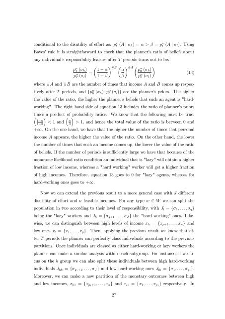
conditional to the disutility of e¤ort as: p w t (A j h ) = > = p w t (A j l ). Using
Bayes’rule it is straightforward to check that the planner’s ratio of beliefs about
any individual’s responsibility feature after T periods turns out to be:
p w T ( #B #A
h) 1 p
w
p w T ( l) = 0 ( h )
1 p w 0 ( l )
where #A and #B are the number of times that income A and B comes up respectively
after T periods, and fp w 0 ( h ) ; p w 0 ( l )g are the planner’s priors. The higher
the value of the ratio, the higher the planner’s beliefs that such an agent is "hardw<strong>orking</strong>".
The right hand side of equation 13 includes the ratio of planner’s priors
times a product of probability ratios. We know that the following must be true:
< 1 and > 1, and hence the total value of the ratio is between 0 and
1
1
+1. On the one hand, we have that the higher the number of times that personal
income A appears, the higher the value of the ratio. On the other hand, the lower
the number of times that such an income comes up, the lower the value of the ratio
of beliefs. If the number of periods is su¢ ciently large we have that because of the
monotone likelihood ratio condition an individual that is "lazy" will obtain a higher
fraction of low income, whereas a "hard w<strong>orking</strong>" worker will get a higher fraction
of high incomes. Therefore, equation 13 goes to 0 for "lazy" agents, whereas for
hard-w<strong>orking</strong> ones goes to +1.
(13)
Now we can extend the previous result to a more general case with J di¤erent
disutility of e¤ort and n feasible incomes. For any type w 2 W we can split the
population in two according to their level of responsibility, with J l = f 1 ; : : : ; q g
being the "lazy" workers and J h = f q+1 ; : : : ; J g the "hard-w<strong>orking</strong>" ones. Likewise,
we can distinguish between high levels of income x h
= fx p+1 ; : : : ; x n g and
low ones x l = fx 1 ; : : : ; x p g. Then, applying the previous result we know that after
T periods the planner can perfectly class individuals according to the previous
partitions. Once individuals are classed as either hard-w<strong>orking</strong> or lazy workers the
planner can make a similar analysis within each subgroup. For instance, if we focus
on the h group we can also split these individuals between high hard-w<strong>orking</strong>
individuals J hh = f q1 +1; : : : ; J g and low hard-w<strong>orking</strong> ones J lh = f 1 ; : : : ; q1 g.
Moreover, we can make a new partition of the monetary outcomes between high
and low incomes, x h1 = fx p1 +1; : : : ; x n g and x l1 = fx 1 ; : : : ; x p1 g respectively. In
27