Random Processes – Fundamentals 1 Generation of a Random ...
Random Processes – Fundamentals 1 Generation of a Random ...
Random Processes – Fundamentals 1 Generation of a Random ...

Create successful ePaper yourself
Turn your PDF publications into a flip-book with our unique Google optimized e-Paper software.
<strong>Random</strong> <strong>Processes</strong> <strong>–</strong> <strong>Fundamentals</strong><br />
Jan Černock´y and Valiantsina Hubeika, FIT VUT Brno<br />
This practical lab covers fundamental work with random signals, in particular ensemble estimation <strong>of</strong><br />
parameters on the set <strong>of</strong> a number <strong>of</strong> realizations <strong>of</strong> a random process. We will be working with random<br />
processes exclusively in descrete time domain. The theory for this lab can be found in the lecture on<br />
random processes. (see http://www.fit.vutbr.cz/study/courses/ISS/public/en/nah e.pdf).<br />
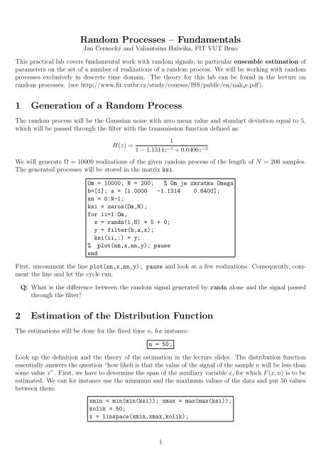
1 <strong>Generation</strong> <strong>of</strong> a <strong>Random</strong> Process<br />
The random process will be the Gaussian noise with zero mean value and standart deviation equal to 5,<br />
which will be passed through the filter with the transmission function defined as:<br />
H(z) =<br />
1<br />
1 − 1.1314z −1 + 0.6400z −2<br />
We will generate Ω = 10000 realizations <strong>of</strong> the given random process <strong>of</strong> the length <strong>of</strong> N = 200 samples.<br />
The generated processes will be stored in the matrix ksi.<br />
Om = 10000; N = 200; % Om je zkratka Omega<br />
b=[1]; a = [1.0000 -1.1314 0.6400];<br />
nn = 0:N-1;<br />
ksi = zeros(Om,N);<br />
for ii=1:Om,<br />
x = randn(1,N) * 5 + 0;<br />
y = filter(b,a,x);<br />
ksi(ii,:) = y;<br />
% plot(nn,x,nn,y); pause<br />
end<br />
First, uncomment the line plot(nn,x,nn,y); pause and look at a few realizations. Consequently, comment<br />
the line and let the cycle run.<br />
Q: What is the difference between the random signal generated by randn alone and the signal passed<br />
through the filter?<br />
2 Estimation <strong>of</strong> the Distribution Function<br />
The estimations will be done for the fixed time n, for instance:<br />
n = 50;<br />
Look up the definition and the theory <strong>of</strong> the estimation in the lecture slides. The distribution function<br />
essentially answers the question “how likeli is that the value <strong>of</strong> the signal <strong>of</strong> the sample n will be less than<br />
some value x”. First, we have to determine the span <strong>of</strong> the auxiliary variable x, for which F (x, n) is to be<br />
estimated. We can for instance use the minumun and the maximum values <strong>of</strong> the data and put 50 values<br />
between them:<br />
xmin = min(min(ksi)); xmax = max(max(ksi));<br />
kolik = 50;<br />
x = linspace(xmin,xmax,kolik);<br />
1
now we can do the estimation:<br />
Fx = zeros(size(x));<br />
for ii = 1:kolik,<br />
thisx = x(ii);<br />
% vybereme vsechna pozorovani pro prislusny cas:<br />
ksin = ksi(:,n);<br />
% a pocitame odhad Fx jako pomer tech, co jsou pod x a vsech:<br />
Fxn(ii) = sum(ksin < thisx) / Om;<br />
end<br />
% vysledek<br />
subplot(211); plot (x,Fxn);<br />
Q: What does the following line <strong>of</strong> code mean Fxn(ii) = sum(ksin < thisx) / Om; If this is not<br />
clear, try to display the result <strong>of</strong> the condition ksin < thisx<br />
Q: Does the distribution function satisfy the theoretical assumption (0 for −∞, 1 for +∞) ?<br />
Q: How would you calculate the probability <strong>of</strong> the random variable an time n lying in the interval<br />
[-10, 5] ?<br />
Q: Calculate F (x, n) at different time n (e.g. 100). Is the value the same ? Can we state that the signal<br />
is stationary ?<br />
3 Estimation <strong>of</strong> the Probability Density Function<br />
p(x, n) will be realized using histogram, again for the fixed time n:<br />
Q: Verify that � ∞<br />
−∞ p(x, n)dx = 1.<br />
deltax = x(2) - x(1);<br />
pxn = hist(ksin,x) / Om / deltax;<br />
subplot(212); plot (x,pxn);<br />
Q: Why do the histogram has to be devided by ∆x and Ω ?<br />
Q: How would you canculate the probability that the random variable at time n lie within the interval<br />
[-10, 5] ?<br />
Q: Calculate p(x, n) for a different time n (e.g.. 100). Is the probability the same? Can we state that<br />
the sinal is stationary?<br />
4 Mean Value and Standard Deviation<br />
For the fixed time n the values are:<br />
an = mean(ksin)<br />
stdn = std(ksin)<br />
For the computation <strong>of</strong> the mean value and the standard deviation at all time points n we will use the<br />
fact that the functions mean and std calculate through columns:<br />
Q: According to you, is the signal stationary ?<br />
aalln = mean(ksi);<br />
stdalln = std(ksi);<br />
subplot(211); plot (nn,aalln);<br />
subplot(212); plot (nn,stdalln);<br />
Q: Why do we see odd values <strong>of</strong> the first few samples <strong>of</strong> the standard deviation?<br />
2
5 Probability Density Function withing a Time Interval, Autocorrelation<br />
Coefficients<br />
Autocorrelation coefficient R(n1, n2) indicates, how “the signal at time n1 is similar with the same signal<br />
at time n2”. The coefficient is calculated as:<br />
R(n1, n2) =<br />
� +∞ � +∞<br />
−∞<br />
−∞<br />
x1x2p(x1, x2, n1, n2)dx1dx2,<br />
thus we need to calculate 2-dimensional probability density function in the time interval from n1 to n2<br />
which will be estimated using a 2-D histogram. Calculation <strong>of</strong> the histogram, approximation to the 2-<br />
D probability density function and calculation <strong>of</strong> the autocorrelation coefficients is implemented in the<br />
function hist2opt (don’t use the function hist2 <strong>–</strong> reference in the lecture slides). An example for n1 = 50<br />
and n2 = n1 + 0 . . . + 20:<br />
n1 = 50;<br />
for n2 = n1:n1+20;<br />
[h,p,r] = hist2opt(ksi(:,n1),ksi(:,n2),x);<br />
imagesc (x,x,p); axis xy; colorbar; xlabel(’x2’); ylabel(’x1’);<br />
[n1 n2 r]<br />
pause<br />
end<br />
Q: Look at the shape <strong>of</strong> the 2-D probabilty density function and try to figure how the signal at times<br />
n1 and n2 is correlated. Look at the value <strong>of</strong> the autocorrelation coeffcient. Does it correspond to<br />
your assumtion?<br />
Q: Why is the value R(50, 50) the highest?<br />
Q: Store the autocorrelation coefficients for all n2 = n1 + 0 . . . + 20: to a vector and diplay it. Describe<br />
what you see.<br />
Q: Display the impuls response <strong>of</strong> the filter the random signal was passed through:<br />
plot(filter(b,a,[1 zeros(1,255)]))<br />
compare the course <strong>of</strong> the autocorrelation coefficients. What is your impression?<br />
Q: Calculate the autocorrelation coefficients for different n1, e.g. n1 = 100 and again with n2 =<br />
n1 + 0 . . . + 20. Is the signal stationary ?<br />
Time Estimation, Spektra<br />
This part <strong>of</strong> the exercise covers fundamental operations on random signals, in particular time estimation<br />
<strong>of</strong> the parameters within one realization <strong>of</strong> the random process We will be working with random processes<br />
exclusively in descrete time domain. The theory for this lab can be found in the lecture on random<br />
processes II. (http://www.fit.vutbr.cz/study/courses/ISS/public/en/nah2 e.pdf).<br />
3
6 <strong>Random</strong> Process <strong>Generation</strong><br />
We will use the same random process as in the first parf <strong>of</strong> the exercise, thus Gaussian noise passed through<br />
the filter<br />
H(z) =<br />
1<br />
1 + −1.1314z−1 ,<br />
+ 0.6400z−2 We will be using only one realization <strong>of</strong> it which will be much longer though: 10000 samples:<br />
N = 10000;<br />
b=[1]; a = [1.0000 -1.1314 0.6400];<br />
nn = 0:N-1;<br />
aux = randn(1,N) * 5 + 0;<br />
x = filter(b,a,aux);<br />
plot (nn,x);<br />
7 Estimation <strong>of</strong> Mean Value and Standard Deviation<br />
. . . is very simple:<br />
a = mean(x)<br />
sigma = std(x)<br />
Q: Did you get the same (approximatelly) values as in the first part <strong>of</strong> the exercise? If so, the signal is<br />
called ergodic, where the ensemble estimates can be replased by temporal estimates (“what can be<br />
estimated from a set <strong>of</strong> signals can be estimated on a single example <strong>of</strong> the signal”)<br />
8 Calculation <strong>of</strong> Distribution Function and Probability Density<br />
Function<br />
similar as in the first part, we will be using one available sample <strong>of</strong> the signal. The signal is denoted as x,<br />
the auxiliary variable is denoted as g:<br />
gmin = min(min(x)); gmax = max(max(x));<br />
% budeme chtit 50 bodu:<br />
number\_<strong>of</strong>\_samples = 50;<br />
g = linspace(gmin,gmax,number\_<strong>of</strong>\_samples);<br />
% a jedeme<br />
Fg = zeros(size(g));<br />
for ii = 1:number\_<strong>of</strong>\_samples,<br />
% a pocitame odhad Fg jako pomer tech, co jsou pod g a vsech:<br />
thisg = g(ii);<br />
Fg(ii) = sum(x < thisg) / N;<br />
end<br />
% vysledek<br />
subplot(211); plot (g,Fg);<br />
Q: Does the distribution function look similar as in the previous example?<br />
Along with the distribution function we will try to generate a Gaussian distribution with the precalculated<br />
mean value and standard deviation. Does the Gaussian correspond to our distribution? The<br />
Gaussian is defined as:<br />
p(g) = 1<br />
σ √ [x−a]2<br />
e− 2σ<br />
2π 2<br />
4
deltag = g(2) - g(1);<br />
pg = hist(x,g) / N / deltag;<br />
% teoreticka Gaussovka<br />
pggaus=1/sqrt(2*pi)/sigma * exp(-(g - a).^2./(2*sigma.^2));<br />
subplot(212); plot (g,pg,g,pggaus);<br />
Q: Can we state that the signal is Gaussian ?<br />
Q: Try to verify (similarly as in the previous task) that � ∞<br />
−∞ p(g)dg = 1.<br />
9 Estimation <strong>of</strong> Autocorrelation Coefficients<br />
Depending on whether devided by the overall number <strong>of</strong> samples or only by the number <strong>of</strong> overlapping<br />
samples, we define biased or unbiased estimation, respectivelly:<br />
ˆRv(k) = 1<br />
N−1 �<br />
x[n]x[n + k],<br />
N<br />
n=0<br />
ˆ Rnv(k) =<br />
In Matlab, we call function xcorr with option ’biased’ or ’unbiased’:<br />
N−1<br />
1 �<br />
x[n]x[n + k],<br />
N − |k|<br />
n=0<br />
Rv = xcorr(x,’biased’); k = -N+1:N-1;<br />
subplot(211); plot(k,Rv)<br />
Rnv = xcorr(x,’unbiased’); k = -N+1:N-1;<br />
subplot(212); plot(k,Rnv);<br />
Q: Why the boundry values <strong>of</strong> the unbiased signal look ’strange’?<br />
Q: Why the boundry values <strong>of</strong> the biased signal are small?<br />
Q: Check whether the value <strong>of</strong> the zero’th autocorrelation coefficient ( in vectors Rv, Rnv it is in the<br />
middle) is equal to the average power <strong>of</strong> the signal:<br />
Ps = 1<br />
N−1 �<br />
x<br />
N<br />
2 [n]<br />
10 Power Spectral Density (PSD)<br />
will be estimated using DFT either from one samples or as a average from a set <strong>of</strong> samples. Averaging<br />
should be leading to a smoother estimation.<br />
10.1 Estimation from One Sample<br />
n=0<br />
N = 10000;<br />
Gdft = 1/N * abs(fft(x)).^2;<br />
om = (0:N/2-1)/N * 2*pi; Gdft = Gdft(1:N/2);<br />
subplot(211); plot (om,Gdft); grid;<br />
Q: What do you think about the estimate? Does it look reasonable?<br />
10.2 Estimation from a Set <strong>of</strong> Samples<br />
will be done by functon gprum.m (you will also need function trame.m 1 , which will devide the signal to<br />
segments with length <strong>of</strong> 100 and estimate PSD for each <strong>of</strong> the segments and then average them:<br />
Q: What do you think about this estimate?<br />
1 Segments are sometimes called frames<br />
[Gprum,om] = gprum(x);<br />
subplot(212); plot (om,Gprum); grid;<br />
5
11 Passing <strong>of</strong> a random signal through a liniar system<br />
Pass the signal through the filter with the transmission function:<br />
H(z) = 1 − 1.1314z −1 + 0.6400z −2<br />
(notice that the filter is the inverse to the filter we generated the signal with). PWD is:<br />
which we will verify by:<br />
Gy(e jω ) = |H(e jω )| 2 Gx(e jω ),<br />
% puvodni PSD - tu mame, ale pro uplnost ...<br />
[Gx,om] = gprum(x);<br />
subplot(131); plot(om,Gx); grid;<br />
% filtr - freq. char na druhou:<br />
a=[1]; b = [1.0000 -1.1314 0.6400];<br />
[h,om] = freqz (b,a,50,2*pi);<br />
h2 = abs(h).^2;<br />
subplot(132); plot(om,h2); grid;<br />
% filtrujeme a zobrazime psd vystupu<br />
% a jeste teoreticky vstupni spek,. hust. vykonu nasobenou<br />
% druhou mocninou H<br />
y = filter(b,a,x);<br />
[Gy,om] = gprum(y); Gyteor = Gx .* h2’;<br />
subplot(133); plot(om,Gy, om, Gyteor); grid;<br />
Q: Does the equation hold Gy(e jω ) = |H(e jω )| 2 Gx(e jω ) ?<br />
Q: Why PSD <strong>of</strong> the output signal is (approximatelly) constant ?<br />
Q: How is such signal called? (white light has a constant spectrum).<br />
Q: Only the zeroth correlation coefficient <strong>of</strong> such random should be nonzero. Verify.<br />
6