Random Processes – Fundamentals 1 Generation of a Random ...
Random Processes – Fundamentals 1 Generation of a Random ...
Random Processes – Fundamentals 1 Generation of a Random ...

Create successful ePaper yourself
Turn your PDF publications into a flip-book with our unique Google optimized e-Paper software.
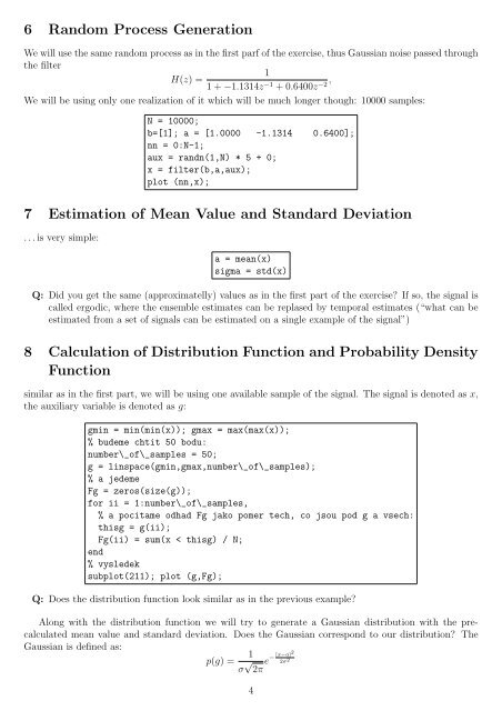
6 <strong>Random</strong> Process <strong>Generation</strong><br />
We will use the same random process as in the first parf <strong>of</strong> the exercise, thus Gaussian noise passed through<br />
the filter<br />
H(z) =<br />
1<br />
1 + −1.1314z−1 ,<br />
+ 0.6400z−2 We will be using only one realization <strong>of</strong> it which will be much longer though: 10000 samples:<br />
N = 10000;<br />
b=[1]; a = [1.0000 -1.1314 0.6400];<br />
nn = 0:N-1;<br />
aux = randn(1,N) * 5 + 0;<br />
x = filter(b,a,aux);<br />
plot (nn,x);<br />
7 Estimation <strong>of</strong> Mean Value and Standard Deviation<br />
. . . is very simple:<br />
a = mean(x)<br />
sigma = std(x)<br />
Q: Did you get the same (approximatelly) values as in the first part <strong>of</strong> the exercise? If so, the signal is<br />
called ergodic, where the ensemble estimates can be replased by temporal estimates (“what can be<br />
estimated from a set <strong>of</strong> signals can be estimated on a single example <strong>of</strong> the signal”)<br />
8 Calculation <strong>of</strong> Distribution Function and Probability Density<br />
Function<br />
similar as in the first part, we will be using one available sample <strong>of</strong> the signal. The signal is denoted as x,<br />
the auxiliary variable is denoted as g:<br />
gmin = min(min(x)); gmax = max(max(x));<br />
% budeme chtit 50 bodu:<br />
number\_<strong>of</strong>\_samples = 50;<br />
g = linspace(gmin,gmax,number\_<strong>of</strong>\_samples);<br />
% a jedeme<br />
Fg = zeros(size(g));<br />
for ii = 1:number\_<strong>of</strong>\_samples,<br />
% a pocitame odhad Fg jako pomer tech, co jsou pod g a vsech:<br />
thisg = g(ii);<br />
Fg(ii) = sum(x < thisg) / N;<br />
end<br />
% vysledek<br />
subplot(211); plot (g,Fg);<br />
Q: Does the distribution function look similar as in the previous example?<br />
Along with the distribution function we will try to generate a Gaussian distribution with the precalculated<br />
mean value and standard deviation. Does the Gaussian correspond to our distribution? The<br />
Gaussian is defined as:<br />
p(g) = 1<br />
σ √ [x−a]2<br />
e− 2σ<br />
2π 2<br />
4