Random Processes – Fundamentals 1 Generation of a Random ...

More documents

Recommendations

Info

6 Random Process Generation We will use the same random process as in the first parf of the exercise, thus Gaussian noise passed through the filter H(z) = 1 1 + −1.1314z−1 , + 0.6400z−2 We will be using only one realization of it which will be much longer though: 10000 samples: N = 10000; b=[1]; a = [1.0000 -1.1314 0.6400]; nn = 0:N-1; aux = randn(1,N) * 5 + 0; x = filter(b,a,aux); plot (nn,x); 7 Estimation of Mean Value and Standard Deviation . . . is very simple: a = mean(x) sigma = std(x) Q: Did you get the same (approximatelly) values as in the first part of the exercise? If so, the signal is called ergodic, where the ensemble estimates can be replased by temporal estimates (“what can be estimated from a set of signals can be estimated on a single example of the signal”) 8 Calculation of Distribution Function and Probability Density Function similar as in the first part, we will be using one available sample of the signal. The signal is denoted as x, the auxiliary variable is denoted as g: gmin = min(min(x)); gmax = max(max(x)); % budeme chtit 50 bodu: number\_of\_samples = 50; g = linspace(gmin,gmax,number\_of\_samples); % a jedeme Fg = zeros(size(g)); for ii = 1:number\_of\_samples, % a pocitame odhad Fg jako pomer tech, co jsou pod g a vsech: thisg = g(ii); Fg(ii) = sum(x < thisg) / N; end % vysledek subplot(211); plot (g,Fg); Q: Does the distribution function look similar as in the previous example? Along with the distribution function we will try to generate a Gaussian distribution with the precalculated mean value and standard deviation. Does the Gaussian correspond to our distribution? The Gaussian is defined as: p(g) = 1 σ √ [x−a]2 e− 2σ 2π 2 4
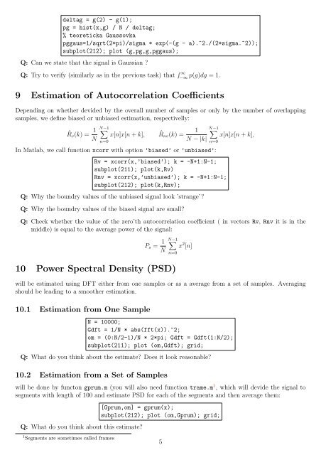
deltag = g(2) - g(1); pg = hist(x,g) / N / deltag; % teoreticka Gaussovka pggaus=1/sqrt(2*pi)/sigma * exp(-(g - a).^2./(2*sigma.^2)); subplot(212); plot (g,pg,g,pggaus); Q: Can we state that the signal is Gaussian ? Q: Try to verify (similarly as in the previous task) that � ∞ −∞ p(g)dg = 1. 9 Estimation of Autocorrelation Coefficients Depending on whether devided by the overall number of samples or only by the number of overlapping samples, we define biased or unbiased estimation, respectivelly: ˆRv(k) = 1 N−1 � x[n]x[n + k], N n=0 ˆ Rnv(k) = In Matlab, we call function xcorr with option ’biased’ or ’unbiased’: N−1 1 � x[n]x[n + k], N − |k| n=0 Rv = xcorr(x,’biased’); k = -N+1:N-1; subplot(211); plot(k,Rv) Rnv = xcorr(x,’unbiased’); k = -N+1:N-1; subplot(212); plot(k,Rnv); Q: Why the boundry values of the unbiased signal look ’strange’? Q: Why the boundry values of the biased signal are small? Q: Check whether the value of the zero’th autocorrelation coefficient ( in vectors Rv, Rnv it is in the middle) is equal to the average power of the signal: Ps = 1 N−1 � x N 2 [n] 10 Power Spectral Density (PSD) will be estimated using DFT either from one samples or as a average from a set of samples. Averaging should be leading to a smoother estimation. 10.1 Estimation from One Sample n=0 N = 10000; Gdft = 1/N * abs(fft(x)).^2; om = (0:N/2-1)/N * 2*pi; Gdft = Gdft(1:N/2); subplot(211); plot (om,Gdft); grid; Q: What do you think about the estimate? Does it look reasonable? 10.2 Estimation from a Set of Samples will be done by functon gprum.m (you will also need function trame.m 1 , which will devide the signal to segments with length of 100 and estimate PSD for each of the segments and then average them: Q: What do you think about this estimate? 1 Segments are sometimes called frames [Gprum,om] = gprum(x); subplot(212); plot (om,Gprum); grid; 5
Page 1 and 2: Random Processes - Fundamentals Jan
Page 3: 5 Probability Density Function with

Random Processes – Fundamentals 1 Generation of a Random ...

You also want an ePaper? Increase the reach of your titles

Delete template?

Save as template?