Modified KPSS Tests for Near Integration - Department of ...
Modified KPSS Tests for Near Integration - Department of ...
Modified KPSS Tests for Near Integration - Department of ...

You also want an ePaper? Increase the reach of your titles
YUMPU automatically turns print PDFs into web optimized ePapers that Google loves.
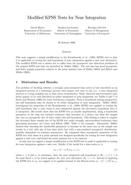
Modi…ed <strong>KPSS</strong> <strong>Tests</strong> <strong>for</strong> <strong>Near</strong> <strong>Integration</strong><br />
David Harris<br />
<strong>Department</strong> <strong>of</strong> Economics<br />
University <strong>of</strong> Melbourne<br />
Stephen Leybourne<br />
School <strong>of</strong> Economics<br />
University <strong>of</strong> Nottingham<br />
30 January 2006<br />
Abstract<br />
Brendan McCabe<br />
School <strong>of</strong> Management<br />
University <strong>of</strong> Liverpool<br />
This note suggests a simple modi…cation to the Kwiatkowski et al. (1994, <strong>KPSS</strong>) test so that<br />
it is applicable to testing the null hypothesis <strong>of</strong> near integration against a unit root alternative.<br />
The modi…ed <strong>KPSS</strong> test is shown not to su¤er from the asymptotic size distortion problems <strong>of</strong><br />
the original <strong>KPSS</strong> test that are described by Müller (2005). The test also has good asymptotic<br />
and …nite sample properties relative to the point optimal tests <strong>of</strong> Müller (2005) and Elliott and<br />
Müller (2005).<br />
1 Motivation and Results<br />
The problem <strong>of</strong> deciding whether a strongly autocorrelated time series is best described as an<br />
integrated process or a stationary process with largest root near to one (i.e. a near integrated<br />
process) is a long standing one in time series econometrics. Many observed macroeconomic time<br />
series appear to be well described as either integrated or near integrated; see Tables 6 and 7 <strong>of</strong><br />
Stock and Watson (1999) <strong>for</strong> some well-known examples. From a hypothesis testing perspective,<br />
the null hypothesis may be chosen to be either integration or near integration. Müller (2005)<br />
investigated the properties <strong>of</strong> the Kwiatkowski et al. (1994, <strong>KPSS</strong>) test applied to testing the<br />
null hypothesis that a time series is near integrated against the alternative hypothesis that it<br />
is integrated. His results show that the <strong>KPSS</strong> test as usually implemented, using a bandwidth<br />
parameter in the long run variance estimator that increases at a slower rate than the sample<br />
size, has an asymptotic size <strong>of</strong> unity under this null hypothesis. This …nding is taken to explain<br />
the increased …nite sample size <strong>of</strong> the <strong>KPSS</strong> test under strongly autocorrelated stationary data<br />
generating processes, see Caner and Kilian (2001, Table 1) <strong>for</strong> example. Alternately, Müller<br />
showed that choosing the bandwidth parameter to increase at the same rate as the sample size<br />
results in a test with size <strong>of</strong> less than unity but with a non-standard asymptotic distribution,<br />
possibly dependent on nuisance parameters. He compared these asymptotic properties <strong>of</strong> the<br />
<strong>KPSS</strong> test with those <strong>of</strong> a point optimal test designed speci…cally <strong>for</strong> testing <strong>for</strong> near integration<br />
against a unit root, and found the point optimal test to be superior.<br />
In this note we suggest a simple modi…cation to the <strong>KPSS</strong> test to make it applicable to testing<br />
<strong>for</strong> near integration against a unit root. Brie‡y, if the model <strong>for</strong> a time series wt is<br />
wt = (1 c=T ) wt 1 + t (1)<br />
where c 0 and t is stationary, then the near integrated null hypothesis is H0 : c c > 0<br />
<strong>for</strong> some …xed c, to be tested against the unit root alternative H1 : c = 0. Instead <strong>of</strong> applying<br />
the <strong>KPSS</strong> test to wt, we suggest it be applied instead to the …ltered series wt (1 c=T ) wt 1.<br />
1
This has the e¤ect <strong>of</strong> removing the near unit root under the null hypothesis, resulting in a <strong>KPSS</strong><br />
test with controlled asymptotic size. Under the alternative hypothesis, the …ltering does not<br />
completely remove the unit root so the test retains non-trivial power.<br />
The asymptotic properties <strong>of</strong> the trans<strong>for</strong>med <strong>KPSS</strong> test are derived and compared with those<br />
<strong>of</strong> the point optimal test <strong>of</strong> Müller (2005) and another point optimal test derived by Elliott and<br />
Müller (2005). These point optimal tests are based on di¤ering treatments <strong>of</strong> the initial value, w1,<br />
in (1). The modi…ed test is found to have superior properties <strong>for</strong> a range <strong>of</strong> assumptions about the<br />
initial value, and also to have superior …nite sample size properties in the presence <strong>of</strong> stationary<br />
autocorrelation in t. We leave <strong>for</strong> future research the use <strong>of</strong> the modi…ed test <strong>for</strong> con…dence<br />
interval construction <strong>for</strong> the largest autoregressive root, as discussed by Elliott and Stock (2001)<br />
using point optimal tests.<br />
2 The Model and Modi…ed <strong>KPSS</strong> Test<br />
Consider the following DGP (cf. Müller and Elliott, 2003) <strong>for</strong> an observed series yt<br />
yt = + wt; t = 1; : : : ; T; (2)<br />
wt = c;T wt 1 + t; t = 2; : : : ; T;<br />
w1 = ;<br />
where t is a stationary process. Here c;T = 1 cT 1 , c 0. We wish to test the null hypothesis<br />
<strong>of</strong> local to unit root stationarity against the unit root alternative. Following Müller (2005) we<br />
state these as H0 : c c > 0 against H1 : c = 0 where c speci…es the minimal amount <strong>of</strong> mean<br />
reversion under the stationary null hypothesis.<br />
As regards the initial value, which is important under H0, following Müller and Elliott (2003),<br />
we assume that it is …xed and set = !=(1 2 c;T ) 1=2 , <strong>for</strong> c > 0. Here controls the magnitude<br />
<strong>of</strong> the initial value relative to the standard deviation <strong>of</strong> a stationary AR(1) process with parameter<br />
c;T < 1.We assume that t is a zero mean stationary process with …nite autocovariances<br />
E( t t j) = j and long-run variance ! 2 = P 1<br />
j= 1 j which is …nite and non-zero.<br />
We consider the following GLS-type trans<strong>for</strong>mation <strong>of</strong> the yt based on our hypothesized value<br />
c under the stationary null,<br />
yt c;T yt 1 = (1 c;T ) + (wt c;T wt 1)<br />
<strong>for</strong> t = 2; : : : ; T . To use the yt c;T yt 1 as the basis <strong>for</strong> a <strong>KPSS</strong> test we need to make them<br />
invariant to (1 c;T ). So, we utilize the OLS estimator <strong>of</strong> (1 c;T ) given by<br />
PT t=2<br />
mc =<br />
(yt<br />
(T<br />
c;T yt<br />
1)<br />
1)<br />
and calculate the OLS residuals<br />
rc;t = (yt c;T yt 1) mc:<br />
Our modi…ed <strong>KPSS</strong> test is then the standard <strong>KPSS</strong> statistic constructed from the rc;t. That is,<br />
S (c) = T 2 PT t=2 (P t<br />
i=2<br />
rc;i)<br />
2<br />
^! 2 c<br />
Here ^! 2 c is any standard long run variance estimator <strong>of</strong> the <strong>for</strong>m<br />
^! 2 TX 1<br />
c = ^c;0 + 2<br />
j=1<br />
(j=l)^ c;j, ^ c;j = T 1<br />
2<br />
TX<br />
t=j+1<br />
rc;trc;t j (3)
where (:) is a kernel function. The following Theorem provides the asymptotic distribution <strong>of</strong><br />
S (c) under the null and alternative hypotheses.<br />
Theorem 1 Under the above assumption <strong>for</strong> t,<br />
where<br />
S (c) )<br />
Z 1<br />
H ;c;c(r)<br />
0<br />
2 dr<br />
Z r<br />
Z 1<br />
H ;c;c(r) = K ;c(r) + c K ;c(s)ds rfK ;c(1) + c K ;c(s)dsg;<br />
K ;c(r) =<br />
(e<br />
0<br />
0<br />
rc 1)(2c) 1=2 + R r<br />
0 e (r s)c W (r);<br />
dW (s); c > 0<br />
c = 0<br />
and W (r) is a standard Wiener process. Also, when c = c > 0, H ;c;c(r) = W (r) rW (1).<br />
The second part <strong>of</strong> the Theorem shows that S (c) has the standard intercept case <strong>KPSS</strong> limiting<br />
null distribution. Note that S (c) is invariant to the initial value even in …nite samples. 1<br />
The modi…ed <strong>KPSS</strong> test is related to the prewhitened long run variance estimator suggested<br />
by Sul, Phillips and Choi (2005) <strong>for</strong> the <strong>KPSS</strong> test. Instead <strong>of</strong> the usual …xed upper bound <strong>of</strong><br />
0.97 <strong>for</strong> the AR(1) prewhitening coe¢ cient, they suggest using 1 T 1=2 . The di¤erence is that<br />
our AR(1) …ltering uses 1 cT 1 and this is employed in both numerator and denominator <strong>of</strong> the<br />
test. Sul, Phillips and Choi (2005) note that the rate T 1 at which 1 cT 1 approaches unity<br />
makes it inappropriate <strong>for</strong> prewhitening when used in the denominator alone, but clearly it is<br />
valid in our context.<br />
3 Comparisons with Optimal Stationarity <strong>Tests</strong><br />
We compare the asymptotic per<strong>for</strong>mance <strong>of</strong> S (c) with that <strong>of</strong> the stationarity test <strong>of</strong> Müller<br />
(2005), denoted Q (g) in the notation <strong>of</strong> that paper (with g corresponding to c) . This test is<br />
asymptotically optimal in a Gaussian setting when g = c, in the situation where the initial value<br />
is generated with = 1. The test was originally suggested as point optimal test <strong>of</strong> the unit root<br />
null in Elliott (1999) but can equally be considered as a test <strong>of</strong> the null <strong>of</strong> stationarity, simply by<br />
considering the opposite tail <strong>of</strong> the distribution to the unit root case.<br />
When testing the unit root null, Müller and Elliott (2003) consider the e¤ect that the magnitude<br />
<strong>of</strong> the initial value in a stationary series has on the power <strong>of</strong> unit root tests. In the<br />
current context <strong>of</strong> stationarity testing, this translates into an issue <strong>of</strong> size control. Elliott and<br />
Müller (2005), in the unit root testing context, derive an asymptotically optimal test (based on a<br />
weighted average power criterion) whose power varies little across di¤erent initial values. Again,<br />
it can equally be considered as stationarity tests, where size should be fairly robust across di¤ering<br />
initial values. We denote this test Q (g; k). As regards choosing parameters, we follow the<br />
previous authors and set c = g = 10 (k = 3:8).<br />
Limit distributions <strong>of</strong> the three statistics are simulated by approximating the Wiener process<br />
functionals involved using i.i.d.N(0; 1) variables, approximating the integrals by normalized sums<br />
<strong>of</strong> 5000 steps. All experiments are based on 10000 replications.<br />
As in Müller (2005), we compare the tests by determining critical values <strong>for</strong> each such that<br />
rejection rates coincide at some prespeci…ed value <strong>for</strong> c = 0 (power) and then examining their size<br />
1 If (2) also includes a linear trend term, the modi…ed statistic is <strong>for</strong>med from the OLS detrended yt c;T yt 1,<br />
t = 2; : : : ; T . Rede…ning rc;t accordingly, the analogue to Theorem 1 follows by replacing H ;c;c(r) with H ;c;c(r)<br />
6r(1 r) R 1<br />
H 0 ;c;c(s)ds. Also, S (c) has the usual trend case <strong>KPSS</strong> distribution.<br />
3
<strong>for</strong> c > 0. In this way, one test dominates another if the <strong>for</strong>mer’s rejection pro…le <strong>for</strong> c > 0 (size)<br />
lies consistently below that <strong>of</strong> the latter. 2<br />
Figure 1 shows the rejection pro…les <strong>of</strong> the tests across c <strong>for</strong> a rejection rate <strong>of</strong> 0.50 when<br />
c = 0. When = 1, Q (10) is the optimal test so it dominates the other two tests everywhere.<br />
Between Q (10; 3:8) and S (10), it is Q (10; 3:8) which dominates, though not substantially. In<br />
fact, there is only ever a very modest amount <strong>of</strong> di¤erence between the size <strong>of</strong> all the three tests,<br />
with all having size close to zero when c = 10. The size <strong>of</strong> each test is also monotonic decreasing<br />
in c. For > 1, the rejection pro…les are no longer monotonic in c. There is always a region <strong>of</strong><br />
c <strong>for</strong> which the size <strong>of</strong> each test is greater than power. However, this e¤ect di¤ers signi…cantly<br />
across tests. As increases the size <strong>of</strong> Q (10) rapidly approaches 1.00 <strong>for</strong> most c, demonstrating<br />
its sensitivity to departures <strong>of</strong> the initial value from its optimality point. The other two tests sizes<br />
appear much less sensitive to increasing . Between these two, while there is virtually nothing<br />
to choose <strong>for</strong> = 2, <strong>for</strong> all 3 it is S (10) that clearly dominates Q (10; 3:8) in terms <strong>of</strong><br />
exhibiting the least size distortion .<br />
To compare …nite sample size, we consider the DGP (2) with = 0 and t generated by the<br />
MA(1) model<br />
t = t t 1<br />
with t i.i.d.N(0; 1). For Q (10) and Q (10; 3:8), we follow Müller (2005) and estimate ! 2 using<br />
residuals from an AR(1) regression <strong>of</strong> demeaned yt in place <strong>of</strong> the rc;t in (3). For all tests we use<br />
the QS kernel <strong>for</strong> (:) and employ the automatic bandwidth selection <strong>of</strong> Newey and West (1994).<br />
For T = 200 and c = 10, Table 1 shows the empirical size <strong>of</strong> the tests using nominal 0.05 level<br />
asymptotic null critical values, <strong>for</strong> various values <strong>of</strong> and . 3 Here S (10) controls size quite well<br />
across (note that its size here is invariant to ). In comparison, both Q (10) and Q (10; 3:8)<br />
are oversized <strong>for</strong> = 0:0; 0:6 and undersized <strong>for</strong> = 0:6. The oversizing problems also increase<br />
with the magnitude <strong>of</strong> - and at a drastic rate in the case <strong>of</strong> Q (10), in keeping with what our<br />
asymptotic results would predict.<br />
Overall, our …ndings indicate that despite its optimality, Q (10) is too susceptible to severe<br />
oversizing problems when > 1 to be recommended <strong>for</strong> practical use. While Q (10; 3:8) su¤ers<br />
rather less in this same situation, it is still the case that S (10) generally displays the more<br />
robust size control asymptotically <strong>for</strong> a given level <strong>of</strong> power and also has better …nite sample size<br />
properties. We there<strong>for</strong>e conclude that, in circumstances when there is some uncertainty about<br />
the generation <strong>of</strong> the initial value, the modi…ed <strong>KPSS</strong> test is likely to provide the most dependable<br />
inference <strong>of</strong> those considered here.<br />
Table 1: Empirical sizes at the nominal 0.05 level.<br />
0.0 0.6 0:6<br />
1 3 5 1 3 5 1 3 5<br />
S (10) 0.046 0.046 0.046 0.021 0.021 0.021 0.051 0.051 0.051<br />
Q (10) 0.060 0.592 0.999 0.000 0.000 0.016 0.096 0.711 0.999<br />
Q (10; 3:8) 0.060 0.091 0.130 0.000 0.000 0.000 0.088 0.116 0.149<br />
2 Note that when c = 0 all the tests are invariant to , so that the same critical values apply <strong>for</strong> all .<br />
3 For S (10) this is the standard <strong>KPSS</strong> value <strong>of</strong> 0.460. Unlike S (10), neither Q (10) or Q (10; 3:8) are invariant<br />
to when c = 10. For these two tests we use asymptotic critical values calculated assuming = 1. This is<br />
appropriate <strong>for</strong> Q (10) as = 1 is the value at which it is optimal. Also, it is not unreasonable <strong>for</strong> Q (10; 3:8)<br />
since this test is designed to have critical values that are fairly insensitive to .<br />
4
4 Pro<strong>of</strong> <strong>of</strong> Theorem 1<br />
As the rc;t are invariant to , we can set = 0 without loss <strong>of</strong> generality, so that yt = wt. It also<br />
proves convenient to de…ne zt = wt w1 and rewrite rc;t in the <strong>for</strong>m<br />
Then<br />
T 1=2<br />
tX<br />
i=2<br />
rc;t = (zt c;T zt 1) mc;z;<br />
mc;z =<br />
rc;i = T 1=2<br />
and may write the …rst RHS term <strong>of</strong> (4) as<br />
T 1=2<br />
tX<br />
i=2<br />
P T<br />
t=2 (zt c;T zt 1)<br />
:<br />
(T 1)<br />
tX<br />
(zi c;T zi 1) tT 1 :T 1=2 mc;z (4)<br />
i=2<br />
(zi c;T zi 1) = T 1=2<br />
= T 1=2<br />
tX<br />
(zi f1 cT 1 gzi 1)<br />
i=2<br />
tX<br />
i=2<br />
zi + cT 3=2<br />
= T 1=2 (zt z2) + cT 3=2<br />
on noting that z1 = 0. It is shown in Elliott (1999) that T 1=2 z [rT ] ) !K ;c(r) where K ;c(r) is<br />
de…ned as in the main text and W (r) is the Wiener process de…ned by P [T r]<br />
i=2 i ) !W (r). So,<br />
setting t = [rT ] we …nd that<br />
[rT ]<br />
T 1=2<br />
X<br />
(zi c;T zi 1) ) !fK ;c(r) + c<br />
i=2<br />
For the second RHS term <strong>of</strong> (4), note<br />
Hence,<br />
[rT ] T 1 :T 1=2 mc;z = [rT ] T 1 :<br />
[rT ]<br />
T 1=2<br />
X<br />
i=2<br />
Thus, via the CMT,<br />
) !rfK ;c(1) + c<br />
Z r<br />
T 1=2<br />
T<br />
(T 1)<br />
Z 1<br />
0<br />
0<br />
tX<br />
i=2<br />
tX<br />
i=3<br />
zi 1<br />
K ;c(s)dsg:<br />
zi 1<br />
TX<br />
(zt c;T zt 1)<br />
t=2<br />
K ;c(s)dsg:<br />
Z r<br />
Z 1<br />
rc;i ) ![K ;c(r) + c K ;c(s)ds rfK ;c(1) + c<br />
0<br />
0<br />
= !H ;c;c(r):<br />
T 1<br />
TX<br />
(T 1=2<br />
t=2<br />
tX<br />
rc;i)<br />
i=2<br />
2 ) ! 2<br />
Z 1<br />
H ;c;c(r)<br />
0<br />
2 dr:<br />
5<br />
K ;c(s)dsg]
That ^! 2 c<br />
and so<br />
p<br />
! ! 2 follows simply by noting that, <strong>for</strong> t = 2; :::; T we can write<br />
yt c;T yt 1 = t + (c c)T 1 wt 1<br />
rc;t = t + (c c)T 1 wt 1<br />
= t + op(1):<br />
P T<br />
t=2 f t + (c c)T 1 wt 1g<br />
(T 1)<br />
To show the second part <strong>of</strong> the Theorem note that when c = c > 0 we have, <strong>for</strong> t = 2; :::; T ,<br />
rc;t = (wt c;T wt 1) mc;w<br />
mc;w =<br />
= vt mc;w;<br />
=<br />
P T<br />
t=2 (wt c;T wt 1)<br />
P T<br />
t=2 vt<br />
(T 1)<br />
so rc;t invariant to and using standard results<br />
[rT ]<br />
(T 1)<br />
T 1=2<br />
X<br />
rc;i ) ![W (r) rW (1)]:<br />
i=2<br />
References<br />
Caner, M. and L. Kilian (2001) Size distortions <strong>of</strong> tests <strong>of</strong> the null hypothesis <strong>of</strong> stationarity:<br />
evidence and implications <strong>for</strong> the PPP debate. Journal <strong>of</strong> International Money and Finance,<br />
20, 639–657.<br />
Elliott, G. (1999) E¢ cient tests <strong>for</strong> a unit root when the initial observation is drawn from its<br />
unconditional distribution. International Economic Review, 40, 767–783.<br />
Elliott, G. and U. Müller (2005) Minimizing the impact <strong>of</strong> the initial condition on testing <strong>for</strong> unit<br />
roots. Journal <strong>of</strong> Econometrics, <strong>for</strong>thcoming .<br />
Elliott, G. and J.H. Stock (2001) Con…dence intervals <strong>for</strong> autoregressive coe¢ cients near one.<br />
Journal <strong>of</strong> Econometrics, 103, 155–181.<br />
Kwiatkowski, D., P. Phillips, P. Schmidt and Y. Shin (1992) Testing the null hypothesis <strong>of</strong> stationarity<br />
against the alternative <strong>of</strong> a unit root. Journal <strong>of</strong> Econometrics, 54, 159–178.<br />
Müller, U. (2005) Size and power <strong>of</strong> tests <strong>for</strong> stationarity in highly autocorrelated time series.<br />
Journal <strong>of</strong> Econometrics, 128, 195-213.<br />
Müller, U. and G. Elliott (2003) <strong>Tests</strong> <strong>for</strong> unit roots and the initial condition. Econometrica, 71,<br />
1269–1286.<br />
Newey, W. and K. West (1994) Automatic lag selection in covariance matrix estimation. Review<br />
<strong>of</strong> Economic Studies, 61, 631–653.<br />
Stock, J.H. and M.W. Watson (1999) Business cycle ‡uctuations in U.S. macroeconomic time<br />
series. Chapter 1 in J.B. Taylor and M. Wood<strong>for</strong>d (eds) Handbook <strong>of</strong> Macroeconomics, Volume<br />
1, Elsevier, Amsterdam.<br />
Sul, D., P.C.B. Phillips and C. Choi (2005) Prewhitening bias in HAC estimation. Ox<strong>for</strong>d Bulletin<br />
<strong>of</strong> Economics and Statistics, 67, 517–546.<br />
6
Figure 1: Asymptotic size and power. — — –S (10); - - - - - Q (10); ––––Q (10; 3:8).