Cobweb Theorems with production lags and price forecasting
Cobweb Theorems with production lags and price forecasting
Cobweb Theorems with production lags and price forecasting

You also want an ePaper? Increase the reach of your titles
YUMPU automatically turns print PDFs into web optimized ePapers that Google loves.
COBWEB THEOREMS WITH PRODUCTION LAGS AND PRICE FORECASTING<br />
DANIEL DUFRESNE AND FELISA J. VÁZQUEZ-ABAD<br />
ABSTRACT. The classical cobweb theorem is extended to include <strong>production</strong> <strong>lags</strong> <strong>and</strong> <strong>price</strong><br />
forecasts. Price <strong>forecasting</strong> based on a longer period has a stabilizing effect on <strong>price</strong>s. Longer<br />
<strong>production</strong> <strong>lags</strong> do not necessarily lead to unstable <strong>price</strong>s; very long <strong>lags</strong> lead to cycles of constant<br />
amplitude. The classical cobweb requires elasticity of dem<strong>and</strong> to be greater than that of<br />
supply; this is not necessarily the case in a more general setting, <strong>price</strong> forcasting has a stabilizing<br />
effect. R<strong>and</strong>om shocks are also considered.<br />
Keywords: <strong>Cobweb</strong> theorem; <strong>production</strong> <strong>lags</strong>; stable markets; <strong>price</strong> fluctuations<br />
1. INTRODUCTION<br />
“But surely the cob-web cycle is an oversimplification of reality” (Samuelson [26], p.4). Many<br />
other famous <strong>and</strong> less famous economists must have expressed the same opinion over the past<br />
decades. We propose to bring the cobweb model at least a little closer to reality by introducing<br />
<strong>production</strong> <strong>lags</strong> <strong>and</strong> <strong>price</strong> forecasts into it. The way equilibrium is reached in a theoretical<br />
model should then be better understood. In particular, we ask whether <strong>production</strong> <strong>lags</strong> cause<br />
intstability of <strong>price</strong>s, <strong>and</strong> whether the classical condition for a cobweb to lead to equilibrium<br />
(that elasticity of dem<strong>and</strong> be greater than elasticity of supply) still holds in a more general<br />
model 1 .<br />
There is a considerable literature on business or economic cycles. The cobweb theorem has a<br />
long history, see Ezekiel [11]. We follow Chapter 2 of van Doorn [8] in stating its classical<br />
form. The following assumptions are made:<br />
(A1) supply depends only on the <strong>price</strong> forecast;<br />
(A2) actual market <strong>price</strong> adjusts to dem<strong>and</strong>, so as to eliminate excess dem<strong>and</strong> instantaneously<br />
in the trading period;<br />
(A3) <strong>price</strong> forecast equals most recent observed <strong>price</strong>, <strong>and</strong><br />
(A4) there are no inventories, <strong>and</strong> neither buyers nor sellers have an incentive to speculate.<br />
Let Pt be the market <strong>price</strong> for a unit of commodity at time t. The quantity dem<strong>and</strong>ed at period<br />
t, denoted by Q d t is given by<br />
Q d t = a0 − a1Pt = D(Pt),<br />
while the quantity supplied is<br />
Q s t = b0 + b1 ˆ Pt = S( ˆ Pt),<br />
where ˆ Pt is the <strong>price</strong> forecast (the result of <strong>forecasting</strong> at time t − 1). The conditions a1, b1 > 0<br />
ensure that quantity dem<strong>and</strong>ed decreases <strong>and</strong> quantity supplied increases as functions of <strong>price</strong>.<br />
The assumptions stated above mean that<br />
D(Pt) = S( ˆ Pt) <strong>and</strong> ˆ Pt = Pt−1.<br />
Making the substitutions, it is seen that the <strong>price</strong> sequence follows<br />
1 We take the dem<strong>and</strong> elasticity to be a positive (absolute) value<br />
Pt = − b1<br />
Pt−1 + a0 − b0<br />
. (1)<br />
a1<br />
1<br />
a1
In the classical cobweb model the solution to (1) is then<br />
Pt = (P0 − P ∗ �<br />
) − b1<br />
�t + P<br />
a1<br />
∗ , (2)<br />
where P ∗ is the equilibrium solution to (1), that is,<br />
P ∗ = − b1<br />
P<br />
a1<br />
∗ + a0 − b0<br />
a1<br />
The sequence defined in (2) converges to P ∗ if <strong>and</strong> only if b1 < a1. In words, the condition for<br />
convergence is that minus the slope of dem<strong>and</strong> as a function of <strong>price</strong> be larger than the slope of<br />
supply as a funtion of <strong>price</strong>. Usually, economic modelling assumes that the market is initially<br />
in equilibrium at P ∗ , <strong>and</strong> that an exogenous disturbance results in P0 �= P ∗ . An important<br />
question is whether such disturbances persist or die out; this can be answered by studying the<br />
conditions for convergence of Pt to P ∗ .<br />
We have in mind the <strong>price</strong>s of metals, for instance copper, which have greatly fluctuated <strong>and</strong><br />
shown some appearance of cycles over time. An important aspect of mining is the lag between<br />
the time the decision to increase or decrease <strong>production</strong> is made <strong>and</strong> the time the decision actually<br />
takes effect in the market. It takes several years for a planned new mine to start producing,<br />
<strong>and</strong> this has made some believe that the <strong>lags</strong> themselves may be a main cause of <strong>price</strong> fluctuations.<br />
In this paper, we study models that include <strong>production</strong> <strong>lags</strong> as well as <strong>price</strong> <strong>forecasting</strong>,<br />
the latter based on current <strong>and</strong> past <strong>price</strong>s. Stability means that <strong>price</strong>s converge to an equilibrium<br />
as time passes. R<strong>and</strong>om disturbances will also be included; in those models “stability”<br />
will mean that <strong>price</strong>s have a limit probability distribution (in other words that the <strong>price</strong> process<br />
has a stationary limit).<br />
Stability is not synonymous <strong>with</strong> absence of fluctuations, but it is a property of markets in which<br />
<strong>price</strong> fluctuations tend to dampen over time. By varying the parameters, one can get an idea of<br />
what may generate fluctuations. Is it <strong>production</strong> <strong>lags</strong>? Is it how <strong>price</strong>s are forecast? We look at<br />
those questions in the following sections.<br />
Given <strong>price</strong>s Pt, Pt−1, . . . , let ˆ Pt+ℓ be the <strong>price</strong> forecast used by producers to establish <strong>production</strong><br />
at time t + ℓ. (A more explicit notation would be ˆ Pt,t+ℓ, but we will use the simpler ˆ Pt+ℓ,<br />
as the lag ℓ will be fixed.) The classical cobweb theorem has a lag of one time unit.<br />
The market clearing condition is now<br />
This leads us to study the dynamical system<br />
.<br />
D(Pt+ℓ) = S( ˆ Pt+ℓ). (3)<br />
Pt+ℓ = D −1 ◦ S( ˆ Pt+ℓ). (4)<br />
Important questions are under what conditions this recursion has an equilibrium point, <strong>and</strong> if<br />
so whether Pt converges to it when t → ∞. Once again, such convergence does not exclude<br />
fluctuations, but it does say that perturbations are damped by the system over time.<br />
The classical description of the cobweb theorem (such as the one we gave above) assumes<br />
that the supply <strong>and</strong> dem<strong>and</strong> functions are linear. We will assume that the dem<strong>and</strong> <strong>and</strong> supply<br />
functions are respectively<br />
D(p) = p −d , S(p) = p s , d, s > 0. (5)<br />
One advantage of these functions is that <strong>price</strong> <strong>and</strong> <strong>production</strong> always remain positive, while<br />
linear functions may lead to negative <strong>price</strong>s (see (2)). Tractability is achieved by using the<br />
logarithm of <strong>price</strong>s, as will be shown below. It will be seen that a very important quantity is the<br />
ratio of the elasticities of supply <strong>and</strong> dem<strong>and</strong>, which we denote c = s/d.<br />
2
Let ℓ ∈ {1, 2, . . . } be the <strong>production</strong> lag. We retain assumptions A1, A2 <strong>and</strong> A4, but replace<br />
(A3) <strong>with</strong><br />
(A3 ′ ) the <strong>price</strong> forecast ˆ Pt+ℓ is a weighted geometric average of (Pt−m, . . . , Pt) for some<br />
m ∈ {0, 1, 2, . . . }.<br />
(N.B. In the sequel “ℓ” will always st<strong>and</strong> for lag, <strong>and</strong> m for memory.)<br />
This means<br />
log ˆ Pt+ℓ =<br />
m�<br />
j=0<br />
αj log Pt−j,<br />
where the weights αj add up to 1. Letting πt = log Pt, ˆπt = log ˆ Pt, the log-<strong>price</strong> forecast is<br />
given by<br />
m�<br />
m�<br />
ˆπt+ℓ = αj πt−j , where αj = 1. (6)<br />
j=0<br />
A moving average model has all weights non-negative. Several <strong>forecasting</strong> schemes have been<br />
identified in the literature, though always for ℓ = 1 (see [29] for a brief description). Static<br />
expectations refers to ˆπt+1 = πt, or m = 0; extrapolative expectations means m = 1 <strong>and</strong><br />
α0 > 1, as<br />
α0πt + α1πt−1 = πt + (α01)πt + (1 − α0)πt−1 = πt + (α0 − 1)(πt − ıt−1).<br />
Adaptive expectations refers to<br />
j=0<br />
ˆπt = λˆπt−1 + (1 − λ)πt.<br />
This is the limit case when m → ∞ <strong>and</strong> αm is proportional to λ m , as we explain in Section 2.7.<br />
We call this exponential smoothing. Note that all these schemes are applied to log-<strong>price</strong>, this is<br />
what makes the model tractable.<br />
Van Doorn [8] attributes to Hicks the use of the logarithm of the <strong>price</strong> rather than the <strong>price</strong> itself,<br />
in the context of a one-lag model or one <strong>with</strong> “distributed <strong>lags</strong>”, but the study of such systems<br />
is not carried out mathematically in [8].<br />
Under (5), the market clearing equation (3) reads<br />
From (6) the sequence πt satisfies<br />
πt+ℓ = −c<br />
Pt+ℓ = ( ˆ Pt+ℓ) −s/d . (7)<br />
m�<br />
αjπt−j , c = s/d. (8)<br />
j=0<br />
Since c �<br />
j αj > 0, the unique equilibrium point is π ∗ = 0 or, equivalently, P ∗ = 1. The<br />
solution πt of (8) has the general form (see [12])<br />
�<br />
ℓ+m<br />
πt = bj x t j,<br />
j=1<br />
where (x1, . . . , xℓ+m) are the zeroes of the characteristic polynomial<br />
hℓ,m(x) = x ℓ+m m�<br />
+ c αjx m−j . (9)<br />
The constants bj; j = 1, . . . , ℓ + m may be found from the initial conditions for πt.<br />
Definition 1. The system (8) is said to be stable if limt→∞ πt = π ∗ = 0, given any initial<br />
conditions. Otherwise it is unstable.<br />
3<br />
j=0
If the characteristic polynomial (9) has complex zeroes then πt has oscillatory components,<br />
which means that the sequence may fluctuate around π ∗ even though it eventually converges to<br />
π ∗ . This will happen frequently in our examples.The magnitude of the zeroes will determine<br />
whether the system is stable or not; if all the zeroes of the characteristic polynomial have norm<br />
(modulus) strictly less than one then the system is stable; if at least one zero has norm greater<br />
than or equal to one then the system is unstable. If the zero or zeroes <strong>with</strong> largest norm have<br />
norm precisely equal to 1 then there will be oscillations <strong>with</strong> constant amplitude, at least for<br />
some initial conditions.<br />
The classical form of the cobweb model has ℓ = 1, m = 0 <strong>and</strong> linear supply <strong>and</strong> dem<strong>and</strong><br />
functions. In our setting, the cobweb model <strong>with</strong> ℓ = 1 <strong>and</strong> m = 0 becomes<br />
which gives<br />
Pt = ( ˆ Pt) −s/d = (Pt−1) −s/d ,<br />
πt = −<br />
�<br />
s<br />
� �<br />
πt−1 =<br />
d<br />
− s<br />
d<br />
� t<br />
π0.<br />
In the classical cobweb model the market is stable if, <strong>and</strong> only if, s < d; in other words, stability<br />
occurs if <strong>and</strong> only if, the elasticity of supply is smaller than the elasticity of dem<strong>and</strong>. When this<br />
is the case, πt → π ∗ = 0. This necessary <strong>and</strong> sufficient condition for stability, s < d, is<br />
remarkably simple <strong>and</strong> easy to interpret. We will see that when <strong>lags</strong> <strong>and</strong> <strong>price</strong> forecasts are<br />
introduced the conditions for stablility are no longer so simple.<br />
Chiarella [6] studies a system where expected <strong>price</strong>s follow adaptive expectations, when the<br />
dem<strong>and</strong> curve is linear, while the supply curve is non-linear (<strong>with</strong> a single point of inflexion,<br />
convex to the left, <strong>and</strong> concave to the right, “a fairly general non-linear S-shaped supply function”,<br />
[6], p.383). He then shows that the system is either (1) stable, (2) unstable but cyclical,<br />
or (3) chaotic. These are very interesting results, but we follow a different route.<br />
The paper is organised as follows. Section 2 studies the deterministic models in some detail,<br />
mostly numerically, although some simple results are proved mathematically. This section<br />
avoids the generality of Section 3 but focuses instead on experiments that lead to interesting<br />
patterns <strong>and</strong> related questions, which will be studied more deeply in subsequent sections.<br />
In Section 3 we derive general results on deterministic models trying to answer the questions<br />
raised in Section 2. The models are represented by linear difference equations; stability is<br />
determined by the study of the roots of the characteristic polynomial (9) of those difference<br />
equations. An important tool is Rouché’s Theorem, see below. Our results seem to contradict<br />
the view that <strong>production</strong> <strong>lags</strong>, by themselves, cause instabilities.<br />
In Section 4 we incorporate r<strong>and</strong>omness into (8), in the form of additive <strong>and</strong> multiplicative<br />
noise. This leads to the question of stability of products of r<strong>and</strong>om matrices, a topic that so far<br />
belonged more in physical chaos theory than in economics.<br />
Notation. The set of complex numbers (or “complex plane”) is denoted C. The norm (or<br />
modulus, or absolute value) of z = x + iy (x, y real) is |z| = � x 2 + y 2 , its conjugate is<br />
z = x − iy. The circle <strong>with</strong> centre z <strong>and</strong> radius ρ in C is denoted Cz,ρ; the open disk (or “ball”)<br />
<strong>with</strong> centre z <strong>and</strong> radius ρ is denoted Bz,ρ; the closed disk is denoted Bz,ρ.<br />
We will use Rouché’s Theorem from complex analysis: if φ, ψ are analytic on <strong>and</strong> inside a<br />
closed contour L, <strong>and</strong> |φ(z)| > |ψ(z)| for z ∈ L, then φ <strong>and</strong> φ + ψ have the same number of<br />
zeroes inside L. Here is a first application: whatever the averaging period m <strong>and</strong> the delay ℓ,<br />
there will be instability if the ratio of elasticities c = s/d is large enough.<br />
Theorem 1. Let ℓ ≥ 1, m ≥ 0. There exists 0 < c0 < ∞ such that for all c ≥ c0 the system<br />
defined by (8) is unstable.<br />
4
Proof. Let<br />
g(z) =<br />
m�<br />
αjz m−j ,<br />
<strong>and</strong> thus hℓ,m(z) = z ℓ+m + cg(z). We show that at least one zero of<br />
j=0<br />
zℓ+m + g(z)<br />
c<br />
is outside C0,ρ, for some ρ ≥ 1. There exists ρ ≥ 1 such that |g(z)| ≥ ɛ > 0 for all z ∈ C0,ρ.<br />
Therefore<br />
|g(z)| > |z|ℓ+m<br />
c<br />
on C0,ρ for all c large enough. Apply Rouché’s theorem <strong>with</strong> φ(z) = g(z) <strong>and</strong> ψ(z) = z ℓ+m /c.<br />
Then φ(z) + ψ(z) has the same number of zeroes inside C0,ρ as g(z), that is, at most m. That<br />
leaves at least ℓ zeroes on or outside C0,ρ, implying instability. �<br />
Remark. A superficially more general version of our model would have supply <strong>and</strong> dem<strong>and</strong><br />
functions<br />
D(p) = kd p −d , S(p) = ks p s , d, s > 0. (10)<br />
Consider the change of variables<br />
p = τ ˜p, τ =<br />
� kd<br />
ks<br />
� 1<br />
d+s<br />
, D(p) = σ ˜ D(˜p), S(p) = σ ˜ S(˜p), σ = k s<br />
d+s<br />
d<br />
this is a change in currency together <strong>with</strong> a change in units. It can be verified that<br />
˜D(˜p) = ˜p −d , ˜ S(˜p) = ˜p s .<br />
There is thus no greater generality in (10) than in (5).<br />
2. DETERMINISTIC MODELS: NUMERICAL EXAMPLES<br />
k d<br />
d+s<br />
s ; (11)<br />
In this section we present numerical experiments that illustrate the influence of the parameters<br />
α, c, ℓ <strong>and</strong> m on stability. The patterns observed here will motivate the more general (<strong>and</strong><br />
mathematical) analysis in Section 3. In all the examples we choose erratic initial conditions<br />
πt = (−10) t sin(1/(t + 3)), t = 0, . . . , ℓ + m.<br />
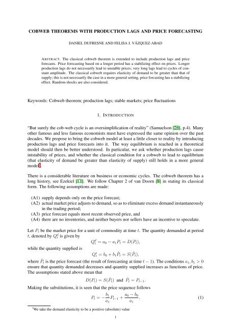
Figure 1 shows the <strong>price</strong> πt as a function of time t when c = 1.7, m = 5, α = (.2, .2, .2, .2, .1, .1),<br />
<strong>and</strong> the delay ℓ takes one of the values ℓ = 2, 3, 4. Notice that c = 1.7 yields instabilities <strong>with</strong><br />
ℓ = 1 (this is the classical cobweb theorem). However, for ℓ = 2 the system is stable, for ℓ = 3<br />
it is nearly periodic <strong>with</strong> constant amplitude, <strong>and</strong> for ℓ = 4 it is unstable. For larger <strong>lags</strong> ℓ ≥ 5<br />
we also observed instability. (However, there is an important comment on this example at the<br />
end of Subsection 3.2.)<br />
1.15<br />
1.10<br />
1.05<br />
1.00<br />
0.95<br />
0.90<br />
0.85<br />
10 20 30 40 50 60 70<br />
(a) ℓ = 2<br />
1.6<br />
1.4<br />
1.2<br />
1.0<br />
10 20 30 40 50 60 70<br />
(b) ℓ = 3<br />
1.8<br />
1.6<br />
1.4<br />
1.2<br />
1.0<br />
0.8<br />
10 20 30 40 50 60 70<br />
(c) ℓ = 4<br />
FIGURE 1. As <strong>production</strong> lag ℓ increases, behaviour changes from stable to unstable.<br />
5
Figure 2 shows the effect of the <strong>forecasting</strong> period m on the <strong>price</strong> behaviour, for c = 1.7<br />
<strong>and</strong> ℓ = 3. The first plot shows the logarithm of <strong>price</strong> πt for m = 1, α = (.7, .3) (the <strong>price</strong><br />
itself soon reaches values larger than 10 6 ). The next plot is the behaviour of πt when m = 5<br />
(α = (.2, .2, .2, .2, .1, .1)) <strong>and</strong> the last one when m = 7 (α = (.2, .1, .1, .1, .1, .1, .1, .1)). These<br />
plots hint at a stabilising effect of increasing m, <strong>and</strong> are consistent <strong>with</strong> other experiments we<br />
made.<br />
10 000<br />
5000<br />
�5000<br />
�10 000<br />
10 20 30 40 50 60 70<br />
(a) m = 1<br />
1.6<br />
1.4<br />
1.2<br />
1.0<br />
10 20 30 40 50 60 70<br />
(b) m = 5<br />
1.2<br />
1.1<br />
1.0<br />
10 20 30 40 50 60 70<br />
(c) m = 7<br />
FIGURE 2. As m increases, behaviour changes from unstable to stable.<br />
In Figure 3 the parameter c is varied, while ℓ = 3, m = 7 <strong>and</strong> α = (.2, .1, .1, .1, .1, .1, .1, .1).<br />
There is apparent stability, except that for the largest value of c there are oscillations of more or<br />
less constant amplitude. The last plot, where c = 3.8 shows nearly cyclical behaviour. Other<br />
experiments (not shown) <strong>with</strong> larger values of c caused the <strong>price</strong>s to diverge. Recall that in the<br />
classical cobweb stability occurs only if c < 1.<br />
1.2<br />
1.1<br />
1.0<br />
10 20 30 40 50 60 70<br />
(a) c = 1.7<br />
1.6<br />
1.4<br />
1.2<br />
1.0<br />
10 20 30 40 50 60 70<br />
(b) c = 3.0<br />
1.8<br />
1.6<br />
1.4<br />
1.2<br />
1.0<br />
0.8<br />
10 20 30 40 50 60 70<br />
(c) c = 3.8<br />
FIGURE 3. As c increases, behavior changes from stable to unstable.<br />
The rest of this section presents detailed discussions of particular cases, that sometimes show<br />
intriguing patterns which, to our knowledge, have not been noted in the context of economic<br />
cycles.<br />
2.1. The case m = 0. Suppose m = 0 <strong>and</strong> ℓ ∈ {1, 2, 3, . . . }. The <strong>price</strong> sequence satisfies<br />
πt+ℓ = −cπt.<br />
(Once again recall that the classical cobweb theorem has m = 0 <strong>and</strong> ℓ = 1.) The solution can<br />
be written as<br />
πkℓ−j = (−c) k π−j , k ∈ {1, 2, . . . }, j ∈ {0, . . . , ℓ − 1}.<br />
Here, there are ℓ <strong>price</strong> dynamics that work “in parallel”, i.e. they are not coupled. Each initial<br />
condition π−j determines πℓ−j, π2ℓ−j <strong>and</strong> so on. If 0 < c < 1 then there are damped oscillations<br />
that tend to zero as k → ∞. If c = 1 then oscillations of same amplitude <strong>and</strong> period 2ℓ persist<br />
endlessly, <strong>and</strong> if c > 1 then the log-<strong>price</strong>s alternate in sign but increase geometrically in size as<br />
time goes by. The role of the ratio of elasticities is clear in this case.<br />
6
2.2. The case ℓ = 1, m = 1.<br />
Theorem 2. Let ℓ = m = 1. Then the sequence πt is stable if, <strong>and</strong> only if, 1 − 1/c < α0 <<br />
1/(2c) + 1/2.<br />
Proof. The solution πt of (8) is stable if, <strong>and</strong> only if, both zeroes of (9) have norm less than 1.<br />
The characteristic polynomial (9) is<br />
h1,1(x) = x 2 + cα0x + cα1 where α1 = 1 − α0.<br />
From Theorem 4.2 of [12], stability for this second order equation is equivalent to the following<br />
three conditions holding simultaneously:<br />
1 + cα0 + c(1 − α0) > 0<br />
1 − cα0 + c(1 − α0) > 0<br />
1 − c(1 − α0) > 0.<br />
Given that c > 0, these are in turn equivalent to 1 − 1/c < α0 < 1/(2c) + 1/2. �<br />
Here the system is unstable for c ≥ 3, because the condition in Theorem 2 cannot then be<br />
satisfied. When ℓ = 1, m = 0, the model is stable only when c < 1, which says that the<br />
elasticity of dem<strong>and</strong> is larger than the elasticity of supply. By contrast, when m = ℓ = 1<br />
stability can be achieved for any c smaller than 3, which means that the elasticity of supply<br />
only needs to be smaller than three times the elasticity of dem<strong>and</strong>. It is somewhat surprising<br />
that increasing the <strong>forecasting</strong> period m from 0 to 1 has such a significant effect. Observe<br />
that the only α0 that produces stability for all c < 3 is 2/3. There is no obvious reason why<br />
it should be α0 = 2/3 that makes this region largest; this corresponds to assigning twice as<br />
much weight to the most recent <strong>price</strong> as the previous one. Note also that if 0 < c < 1 then<br />
1/(2c) + 1/2 > 1, meaning that for those values of c the sequence is stable in particular for<br />
α0 ∈ (1, 1/(2c) + 1/2), which corresponds to establishing the <strong>price</strong> forecast by extrapolating<br />
the two most recent <strong>price</strong>s. For example, if c = 1/2, log Pt = 1, log Pt−1 = 0, α0 = 5/4 then<br />
the forecast is log ˆ Pt+1 = 5/4; the <strong>price</strong> sequence is stable in this case, even though a priori<br />
one might think that extrapolating the most recent <strong>price</strong>s would be a destabilizing policy. In<br />
the economics literature, the expression “extrapolative expectations” refers to <strong>forecasting</strong> based<br />
on the last two <strong>price</strong>s. This idea was first studied mathematically in a macroeconomic model<br />
of inventories by Metzler [19]. Metzler studies a somewhat different problem, but the algebra<br />
is similar to our case ℓ = 1, m = 1. (Metzler <strong>and</strong> others believed that extrapolation was a<br />
cause of instability). Turnovsky [29] mentions the destabilizing effect of extrapolation (i.e.<br />
α0 > 1). Extrapolative expectations is also called a “myopic” forecast by other authors, for<br />
instance Wheaton [32] claims that this is a cause of real estate oscillations.<br />
2.3. The cases m = 1, ℓ ≥ 2, α0 = 0 or 1. When m = 1 <strong>and</strong> ℓ ≥ 2, equation (8) cannot be<br />
solved exactly, except for the two special cases α0 = 0 <strong>and</strong> α0 = 1, which are tractable. In the<br />
first case, the characteristic polynomial is<br />
which has zeros xj <strong>with</strong> norm<br />
hℓ,m(x) = x ℓ+1 + c<br />
|xj| = c 1/(ℓ+1) , j = 1, . . . , ℓ + 1.<br />
Hence the condition c < 1 is a necessary <strong>and</strong> sufficient condition for stability when α0 = 0. In<br />
the case α0 = 1 the zeros of the characteristic polynomial<br />
hℓ,m(x) = x ℓ+1 + cx<br />
are 0 <strong>and</strong> xj = c 1<br />
ℓ e 2π(j−1)<br />
ℓ , j = 1, . . . , ℓ, <strong>and</strong> once again c < 1 is a necessary <strong>and</strong> sufficient<br />
condition for stability.<br />
7
2.4. The cases m = 1, ℓ ≥ 2, α0 arbitrary. The graphs in Figure 4 show the region of stability<br />
for m = 1 <strong>and</strong> ℓ between 1 <strong>and</strong> 100, computed using Mathematica R○ . The stability region<br />
is the set of (α0, c) that lead to a stable <strong>price</strong> sequence; the curves on the graphs are the upper<br />
boundaries of the stability regions. We have observed numerically that the stability region<br />
shrinks to some limit set as ℓ increases, though the shape of the upper boundary is different for<br />
even <strong>and</strong> odd values of ℓ.<br />
2.0<br />
1.5<br />
1.0<br />
0.5<br />
��1<br />
��3<br />
��5<br />
limit<br />
0.0<br />
�3 �2 �1 0 1 2 3<br />
(a) ℓ odd.<br />
2.0<br />
1.5<br />
1.0<br />
0.5<br />
��2<br />
limit<br />
��4 ��6<br />
0.0<br />
�3 �2 �1 0 1 2 3<br />
(b) ℓ even.<br />
FIGURE 4. m = 1. The region of stability is the area below each of the curves shown.<br />
The stability region is largest when ℓ = 1; the upper boundaries for ℓ ≥ 5 are indistinguishable<br />
from the limit when α0 is outside (0, 1). The limit as ℓ tends to infinity of the upper boundary<br />
of the stability region coincides (as far as we can tell numerically) <strong>with</strong> the curve<br />
c = (|α0| + |1 − α0|) −1<br />
(solid line). We give a partial justification in Section 3.<br />
2.5. The case 1 < m < ∞: equal weights αj. In our next numerical experiments the weights<br />
are equal, i.e. αj = 1/(m + 1), j = 0, . . . , m. Hence,<br />
hℓ,m(x) = x ℓ+m + c<br />
m�<br />
x<br />
m + 1<br />
m−j . (12)<br />
Figure 5 plots the supremum of the values of c that preserve stability, that is, the values of<br />
c ∗ �<br />
(ℓ, m) = inf<br />
c>0<br />
max<br />
j∈{1,...,m+ℓ} |xj(c)|<br />
�<br />
= 1 ,<br />
where {xj(c)} are the zeroes of (12). The horizontal axis shows the values of the averaging<br />
period m, <strong>and</strong> the four dotted lines correspond to ℓ = 1, 2, 3, 4. The dotted lines visually appear<br />
to be linear functions of m, <strong>with</strong> a slope that decreases as the lag ℓ increases. A closer look<br />
at the actual values of c ∗ (ℓ, m) shows that for fixed ℓ = 2, 3, 4 the functions are not precisely<br />
linear in m, but for ℓ = 1 the slope is indeed constant.<br />
We are able to prove that if ℓ = 1 then c ∗ (ℓ, m) = m + 1, see Section 3.3.<br />
Figure 6 shows the zeroes of the characteristic polynomial hℓ,m(x) in the complex plane for<br />
m = 6 <strong>and</strong> various values of ℓ. Each number “ℓ” on a plot represents the location of a zero<br />
of hℓ,m(x). It is seen that, at least in those cases, the zeroes move towards the unit circle as<br />
ℓ increases, <strong>and</strong>, furthermore, that the zeroes are approximately uniformly spread around the<br />
8<br />
j=0
10<br />
8<br />
6<br />
4<br />
2<br />
2 4 6 8 10<br />
FIGURE 5. Critical value of the ratio of elasticities c as a function of m. The top<br />
line corresponds to ℓ = 1, the ones below correspond to ℓ = 2, 3, 4 (in that<br />
order).<br />
circle. Intuitively this means that the behaviour of <strong>price</strong>s tends to oscillations when ℓ increases.<br />
We now provide an incomplete justification for this. The characteristic polynomial is<br />
hℓ,m(z) = z ℓ+m m� 1<br />
+ cg(z), g(z) =<br />
z<br />
m + 1<br />
m−j .<br />
Letting w = z ℓ+m , this may be rewritten as Hℓ,m(w) = w + cg(w 1<br />
ℓ+m ).<br />
50 50 50 50 50 50 50<br />
50<br />
50<br />
50<br />
50<br />
10<br />
10<br />
50<br />
50<br />
5<br />
10 50<br />
10 5<br />
50<br />
50<br />
1<br />
5 50<br />
50<br />
10<br />
50<br />
50 10 1<br />
50 5<br />
50<br />
1<br />
50<br />
5 50<br />
10<br />
50 10<br />
50<br />
50<br />
50<br />
5<br />
1<br />
m � 6, c � 0.2<br />
50 10<br />
10<br />
50<br />
50<br />
5 50<br />
50 5<br />
1<br />
10<br />
50<br />
50<br />
1<br />
10<br />
50<br />
50<br />
1<br />
5 50<br />
50<br />
10 5<br />
50<br />
50<br />
5<br />
10 50<br />
50 10<br />
50<br />
10<br />
50<br />
50<br />
50 50 50<br />
50<br />
50 50 50 50<br />
m � 6, c � 2<br />
50 50 50<br />
50 50 50<br />
10 50<br />
5<br />
50<br />
50 10 1<br />
50<br />
50<br />
10 5<br />
1050<br />
50<br />
50<br />
5 50<br />
50<br />
1<br />
1050<br />
50<br />
1<br />
50<br />
50 10<br />
5<br />
505<br />
50<br />
50<br />
50<br />
10<br />
50 10<br />
50<br />
50<br />
50<br />
5 1<br />
50 10<br />
50<br />
50<br />
10<br />
50<br />
50<br />
5<br />
505<br />
50 10<br />
50<br />
50<br />
1<br />
1<br />
1050<br />
50<br />
5 50<br />
50<br />
10<br />
50<br />
50 5<br />
1050<br />
50 10 1<br />
50<br />
5<br />
50<br />
50 50 10 50<br />
50 50 50 50<br />
50<br />
50<br />
50<br />
50<br />
5<br />
1<br />
j=0<br />
50 50 50<br />
50 50 50 50<br />
50<br />
50<br />
10 50<br />
50<br />
10 5<br />
50<br />
50 10 5<br />
1<br />
10 50<br />
50<br />
5 50<br />
50<br />
10 50<br />
1<br />
50<br />
50 10<br />
1<br />
50<br />
5<br />
50<br />
5<br />
50<br />
50<br />
10<br />
50 10<br />
50<br />
50<br />
50<br />
m � 6, c � 0.7<br />
50 10<br />
50<br />
10<br />
50<br />
50<br />
50<br />
5<br />
5<br />
50<br />
50 10<br />
1<br />
1<br />
50<br />
50<br />
10 50<br />
50<br />
5 50<br />
50 10 5<br />
1<br />
10 50<br />
50<br />
10 5<br />
50<br />
50<br />
50<br />
10 50<br />
50 50<br />
50<br />
50 50 50 50<br />
m � 6, c � 3<br />
10<br />
50 50 50<br />
50 50 50 50<br />
5 50<br />
50 10 1<br />
50<br />
50 5<br />
10<br />
1050<br />
50<br />
5 50<br />
50<br />
50 1<br />
1<br />
10<br />
50<br />
50<br />
50<br />
50 10<br />
5<br />
5<br />
50<br />
50<br />
50<br />
50<br />
10<br />
50<br />
10<br />
50<br />
50<br />
5 1<br />
50<br />
50<br />
10<br />
50<br />
50<br />
10<br />
50<br />
50<br />
5<br />
50<br />
50 10<br />
5<br />
50<br />
50<br />
1<br />
1 50<br />
50<br />
10<br />
5<br />
50<br />
50<br />
50<br />
5010<br />
5<br />
1050<br />
50 10<br />
50<br />
1<br />
50<br />
50 50 5 50<br />
50 50<br />
10 50 50<br />
FIGURE 6. Zeroes of the characteristic polynomial hℓ,m(x) for different values<br />
of c, <strong>with</strong> m = 6, in the complex plane. Each zero is indicated by the number<br />
“ℓ”. The circle has centre 0 <strong>and</strong> radius 1 (C0,1).<br />
We now use Rouché’s Theorem <strong>with</strong> φ(z) = cg(z), ψ(z) = z ℓ+m <strong>and</strong> C = C0,ρ, for 0 < ρ < 1.<br />
The zeroes of φ are all on the unit circle, <strong>and</strong> thus |φ(z)| ≥ ɛ > 0 for z ∈ C0,ρ. Hence, for ℓ<br />
larger than some ℓ0 the inequality |φ(z)| > |ψ(z)| is verified for z ∈ C0,ρ; this implies that the<br />
9<br />
50<br />
50<br />
50<br />
50
zeroes of hℓ,m are all outside B0,ρ, for any 0 < ρ < 1. Now w 1<br />
ℓ+m → 1 as ℓ → ∞, <strong>and</strong> we are<br />
left <strong>with</strong><br />
lim<br />
ℓ→∞ Hℓ,m(w) = w + c.<br />
Finally, reverting to w = z ℓ+m then says that the zeroes of hℓ,m are, approximately, the solutions<br />
of<br />
z ℓ+m = −c.<br />
The zeroes are then approximately equal to<br />
c 1 2πj<br />
i ℓ+m e ℓ+m , j = 1, . . . , ℓ + m.<br />
Although not rigorously derived, this yields good approximations of the arguments 2πj/(ℓ + m),<br />
but not always a good one for the norms of the zeroes of hℓ,m. For the latter it is better to rely<br />
on the fact that the norm of the product of the zeroes of hℓ,m is |hℓ,m(0)| = c/(m + 1), which<br />
yields the improved approximation<br />
� c<br />
m + 1<br />
� 1<br />
ℓ+m 2πj<br />
i<br />
e ℓ+m , j = 1, . . . , ℓ + m. (13)<br />
As an example, consider the first graph in Figure 6, <strong>with</strong> equals weights αj = 1/(m+1), c = .2<br />
<strong>and</strong> m = 6. For ℓ = 5 the exact zeroes are rje iθj , <strong>with</strong><br />
r1 = 0.694659, θ1 = 3.14159,<br />
r2 = 0.688829, θ2 = −2.59503, r3 = 0.688829, θ3 = 2.59503,<br />
r4 = 0.700281, θ4 = −2.03232, r5 = 0.700281, θ5 = 2.03232,<br />
r6 = 0.716104, θ6 = −1.49399, r7 = 0.716104, θ7 = 1.49399,<br />
r8 = 0.730140, θ8 = −0.92760, r9 = 0.730140, θ9 = 0.92760,<br />
r10 = 0.804108, θ10 = −0.35203, r11 = 0.804108, θ11 = 0.35203,<br />
while the approximations are re iθj , where r = 0.723819 <strong>and</strong> the θj are<br />
3.14159, ±2.57039, ±1.9992, ±1.428, ±0.856798, ±0.285599.<br />
If (13) were the true zeroes of hℓ,m then the solutions<br />
πt = �<br />
j=1<br />
would have period ℓ + m. In the mining area, many believe that that the observed <strong>price</strong> cycles<br />
correspond to the <strong>production</strong> lag ℓ. We see that this is approximately the case in our model, but<br />
only when m is small.<br />
2.6. Geometric weights. Geometric weights are used in many <strong>forecasting</strong> models. A parameter<br />
λ > 0 is chosen <strong>and</strong> the weights αj follow the geometric progression<br />
bjx t j<br />
αj = λj (1 − λ)<br />
(1 − λm+1 , j = 0, . . . , m. (14)<br />
)<br />
Figure 7 shows plots of the critical boundary value c ∗ as a function of λ for different values of<br />
ℓ, m. In all cases it appears that the stability region decreases to c ∗ = 1 as ℓ increases. The solid<br />
line is the function<br />
˜c(λ) def<br />
= (1 + λ)(1 − λm+1 )<br />
(1 − λ)(1 + λ m+1 ) ,<br />
which is the boundary for the region for ℓ = 1 <strong>and</strong> even values of m, as we will prove in<br />
Section 3.<br />
10
3.0<br />
2.5<br />
2.0<br />
1.5<br />
1.0<br />
0.5<br />
0.0<br />
��1<br />
��2<br />
��3<br />
��4<br />
��5<br />
��10<br />
0.0 0.2 0.4 0.6 0.8 1.0<br />
(a) m = 2<br />
10<br />
8<br />
6<br />
4<br />
2<br />
0<br />
��1<br />
��2<br />
��3<br />
��4<br />
��5<br />
��10<br />
0.0 0.2 0.4 0.6 0.8 1.0<br />
(c) m = 10<br />
6<br />
5<br />
4<br />
3<br />
2<br />
1<br />
0<br />
��1<br />
��2<br />
��3<br />
��4<br />
��5<br />
��10<br />
0.0 0.2 0.4 0.6 0.8 1.0<br />
(b) m = 5<br />
FIGURE 7. Stability regions for geometric weights are shown for different <strong>production</strong><br />
<strong>lags</strong> ℓ.<br />
2.7. Exponential smoothing. If 0 < λ < 1 <strong>and</strong> we formally let m → ∞ in (14), we get<br />
∞�<br />
ˆπt+ℓ = (1 − λ) λ j πt−j.<br />
Rewriting the same for ˆπt+ℓ−1 <strong>and</strong> eliminating πt−1, πt−2, . . . , we then find that<br />
j=0<br />
ˆπt+ℓ = λˆπt+ℓ−1 + (1 − λ)πt.<br />
This says that the forecast made at time t for the <strong>price</strong> at time t + ℓ is a weighted average of<br />
last period’s forecast <strong>and</strong> the most recent <strong>price</strong>, using a fixed proportion λ. This procedure is<br />
mentioned in [8], page 24; it is sometimes called “exponential smoothing” or “adaptive expectations”.<br />
From (7), πt+ℓ = −cˆπt+ℓ <strong>and</strong> thus<br />
The case ℓ = 1 is remarkably simple:<br />
πt+ℓ = λπt+ℓ−1 − c(1 − λ)πt (15)<br />
πt+1 = [(1 + c)λ − c]πt.<br />
By setting<br />
λ = c<br />
=<br />
1 + c<br />
s<br />
d + s ,<br />
one gets πt+1 = 0, i.e. there is convergence to the equilibrium <strong>price</strong> in just one time step.<br />
11
There is an explicit result when ℓ = 2, reminiscent of the case ℓ = 1, m = 1 (Theorem 2).<br />
Theorem 3. If (15) holds <strong>with</strong> c > 0, then<br />
(a) if ℓ = 1, then the sequence πt is stable if, <strong>and</strong> only if, (c − 1)/(c + 1) < λ < 1;<br />
(b) if ℓ = 2, then the sequence πt is stable if, <strong>and</strong> only if, 1 − 1/c < λ < 1.<br />
Proof. For part (a), the condition is<br />
−1 < (1 + c)λ − c < 1 or<br />
For part (b), the zeroes of the characteristic polynomial<br />
x 2 − λx + c(1 − λ)<br />
have norm less than 1 if, <strong>and</strong> only if ([12], p.172),<br />
c − 1<br />
c + 1<br />
< λ < 1.<br />
1 + λ + c(1 − λ) > 0, 1 − λ + c(1 − λ) > 0, 1 − c(1 − λ) > 0.<br />
These are equivalent to 1 − 1/c < λ < 1. �<br />
When ℓ > 2 the characteristic polynomial has degree three or more, <strong>and</strong> an exact analysis of<br />
the roots is not possible. Figure 8 shows the boundary of the stability region as a function of λ.<br />
The solid lines are the functions (1 + λ)/(1 − λ) <strong>and</strong> 1/(1 − λ), <strong>and</strong> coincide numerically <strong>with</strong><br />
ℓ = 1, 2 respectively, as expected.<br />
In all the experiments we made, for any c there is an interval I(c) = (λ(c), 1) such that λ ∈ I(c)<br />
implies stability. We have not been able to prove mathematically that this is always the case<br />
when ℓ ≥ 3.<br />
10<br />
8<br />
6<br />
4<br />
2<br />
0<br />
��1<br />
��2<br />
��5<br />
��10<br />
0.0 0.2 0.4 0.6 0.8 1.0<br />
FIGURE 8. Stability region for exponential smoothing.<br />
12
m � 3, c � 0.2, Α ��0.1, 0.6, 0.2, 0.1�<br />
Im�z�<br />
50<br />
50 50 50 50 50<br />
50<br />
50<br />
10 50<br />
50<br />
50<br />
50 10<br />
5<br />
50<br />
50<br />
10 50<br />
50<br />
50<br />
50<br />
10<br />
10 50 5 1<br />
50<br />
50<br />
5<br />
5<br />
50<br />
50<br />
1<br />
10<br />
50<br />
50<br />
50<br />
50 10<br />
50<br />
50<br />
50<br />
50<br />
1<br />
10<br />
50<br />
5<br />
50<br />
5 1<br />
5<br />
10<br />
10 50<br />
50<br />
50<br />
50<br />
50<br />
50<br />
10 50<br />
5<br />
50 10<br />
50<br />
50<br />
50<br />
10<br />
50<br />
50<br />
50<br />
50<br />
50 50 50 50 50<br />
FIGURE 9. Zeroes of the characteristic polynomial hℓ,m(x) for non-equal<br />
weights, in the complex plane. Each zero is indicated by the number “ℓ”. The<br />
circle has centre 0 <strong>and</strong> radius 1 (C0,1).<br />
2.8. Arbitrary weights. Figure 9 shows the locations of the zeroes in the complex plane in<br />
one case where the weights αj are not equal: α = (0.1, 0.6, 0.2, 0.1), c = 1. The characteristic<br />
polynomial<br />
hℓ,m(z) = z ℓ+3 + 0.2(0.1z 3 + 0.6z 2 + 0.2z + 0.1) = z ℓ+3 + 0.2g(z)<br />
has all its zeroes inside the unit circle C0,1 for all ℓ. This is a simple consequence of the reverse<br />
triangle inequality: if |z| ≥ 1 then<br />
|hℓ,m(z)| ≥ |z ℓ+3 | − 0.2|0.1z 3 + 0.6z 2 + 0.2z + 0.1| ≥ |z| ℓ+3 − 0.2|z| 3 .<br />
The last expression cannot be zero if |z| ≥ 1, for any ℓ = 1, 2, . . . . We note that there are now<br />
ℓ + m − 2 zeroes spread in a circular fashion, getting closer to C0,1 as ℓ increases, as there are<br />
ℓ + m zeroes in total <strong>and</strong> two zeroes that remain near −0.16 ± 0.38i. It will be shown in Section<br />
3 that inside the unit circle the zeroes of hℓ,m have limits as ℓ tends to infinity, <strong>and</strong> that they are<br />
precisely the zeroes of g(z) = �m j=0 αjz m−j (as defined in the proof of Theorem 1).<br />
Re�z�<br />
3. DETERMINISTIC MODELS: GENERAL RESULTS<br />
Let us recall from (3) that for a lag ℓ <strong>and</strong> an averaging period m + 1, the market clearing<br />
condition<br />
P −d<br />
t+ℓ = ˆ P s<br />
t+ℓ,<br />
yields (8), that is<br />
πt+ℓ = − s<br />
m�<br />
αjπt−j.<br />
d<br />
Writing c = s/d as before, the characteristic polynomial (9) is<br />
hℓ,m = x ℓ+m m�<br />
+ c αjx m−j ,<br />
<strong>and</strong> the solution of (8) is<br />
πt =<br />
j=0<br />
j=0<br />
ℓ+m �<br />
bk x t k, (16)<br />
k=1<br />
13
where {xk} are the zeroes of the characteristic polynomial <strong>and</strong> {bk} are constants. The long<br />
term behaviour of πt is determined by the xj <strong>with</strong> the maximum norm, among those j such that<br />
bj �= 0. Analytic expressions for the zeroes of polynomials are not available for l + m > 2, but<br />
we will derive results that narrow down the region where the zeroes are located.<br />
In the literature, some have suggested that <strong>production</strong> <strong>lags</strong> themselves are the cause of fluctuating<br />
<strong>price</strong>s. For example, in [23], p.276, Phillips mentions that “the regulation of a system can be<br />
improved if the lengths of the time delay operating around the main control loop are reduced.”<br />
Sterman ([27], Chapter 20) writes: “markets <strong>with</strong> negative feedbacks through which <strong>price</strong> seeks<br />
to equilibrate supply <strong>and</strong> dem<strong>and</strong> often involve long time delays which lead to oscillation.” Our<br />
results do support this view, but maybe not in the way one might have expected, in the sense<br />
that we do not find that longer <strong>lags</strong> necessarily lead to instability. What we find is that as the<br />
lag ℓ increases the maximum of the norms of the roots xk tends to one. This means oscillations<br />
of constant amplitude, whether the system is stable or unstable for small <strong>production</strong> <strong>lags</strong>. Thus,<br />
longer <strong>lags</strong> have a stabilizing effect on unstable systems. This is the conclusion one draws from<br />
the general results in Subsections 3.1 <strong>and</strong> 3.2. Subsection 3.3 studies the case where the weights<br />
{αj} are constant or form a geometric progression.<br />
3.1. General result on the location of the roots <strong>and</strong> stability.<br />
m�<br />
Theorem 4. (a) Suppose ρ ≥ 1. If c |αj| < ρ ℓ then the zeroes of hℓ,m are all less than ρ in<br />
norm, i.e. |xj| < ρ. In particular, if<br />
then the system is stable.<br />
(b) Suppose ρ ≤ 1. If c<br />
j=0<br />
c<br />
m�<br />
|αj| < 1 (17)<br />
j=0<br />
m�<br />
|αj| < ρ ℓ+m then the zeroes of hℓ,m are all less than ρ in norm.<br />
j=0<br />
Proof. Let ρ ≥ 1 <strong>and</strong> |z| ≥ ρ. Then, from the triangle inequality,<br />
|hℓ,m(z)| ≥ |z| ℓ+m m�<br />
− c |αj||z| m−j ≥ |z| ℓ+m − c|z| m<br />
j=0<br />
m�<br />
|αj|.<br />
If c � m<br />
j=0 |αj| < ρ ℓ then the last expression is positive. The zeroes of hℓ,m must then all be in<br />
C0,ρ.<br />
If ρ ≤ 1 <strong>and</strong> |z| ≥ ρ then the result follows from<br />
|hℓ,m(z)| ≥ |z| ℓ+m m�<br />
− c |αj| ≥ |ρ| ℓ+m − c<br />
j=0<br />
j=0<br />
m�<br />
|αj|. �<br />
Observe that (17) is sufficient for stability, but not necessary. For instance, in the case m = 1<br />
depicted in Figure 4 it is seen that when 0 < α0 < 1 the system is stable for some c > 1 =<br />
α0 + α1.<br />
Part (a) of the theorem implies that for any ρ > 1 <strong>and</strong> for ℓ greater than some ℓ0, the zeroes of the<br />
the characteristic polynomial are all inside C0,ρ. This means that for systems that are unstable<br />
for some ℓ there are larger ℓ’s such that the maximum norm of the zeroes of the characteristic<br />
polynomial is close to 1; in other words, an unstable system eventually becomes less unstable<br />
as ℓ increases.<br />
14<br />
j=0
As an application of Theorem 4, let us now return to the cases m = 1, ℓ ≥ 1, α0 arbitrary, that<br />
we looked at in Section 2 (cf. Figure 4).<br />
Suppose ℓ is odd, <strong>and</strong> fix α0 ≥ 1. If we set c = (|α0| + |1 − α0|) −1 = 1/(2α0 − 1) then<br />
a zero of hℓ,1(x) is x = −1, <strong>and</strong> the system is unstable. However, Theorem 4 says that if<br />
c < (|α0| + |1 − α0|) −1 then the system is stable. Hence, the stability region for ℓ odd, α0 ≥ 1<br />
consists of the points (α0, c) <strong>with</strong> c < (|α0| + |1 − α0|) −1 . The situation is similar when ℓ is<br />
even <strong>and</strong> α0 ≤ 0; then c = (|α0| + |1 − α0|) −1 = 1/(1 − 2α0) leads to a zero at x = −1 again,<br />
while Theorem 4 gives stability when c < 1/(1 − 2α0). Hence, the stability region for ℓ even,<br />
α0 ≤ 0 consists of the points (α0, c) <strong>with</strong> c < (|α0| + |1 − α0|) −1 .<br />
3.2. Limiting behaviour <strong>with</strong> increasing <strong>production</strong> <strong>lags</strong>. The next result shows that when<br />
the <strong>production</strong> lag ℓ increases <strong>with</strong>out bound, all the zeroes of the characteristic polynomial<br />
hℓ,m(x) are arbitrarily close to the unit circle, <strong>with</strong> the possible exception of up to m zeroes<br />
inside the unit circle. This means, loosely speaking, that longer <strong>production</strong> <strong>lags</strong> lead to oscillations<br />
of constant amplitude, <strong>and</strong> not to oscillations of increasing amplitude. A system that has<br />
oscillations of increasing amplitude will be made less unstable for <strong>production</strong> <strong>lags</strong> that are long<br />
enough. This partly contradicts the view that long <strong>production</strong> <strong>lags</strong> in themselves cause erratic<br />
<strong>price</strong> behaviour.<br />
We will use the following classical result from [25], page 261.<br />
Theorem (Hurwitz) Let G be a non-empty connected open set in the complex plane. Suppose<br />
φ, φn, n ≥ 1 are analytic functions on G, <strong>and</strong> that φn converges uniformly on compacts to φ in<br />
G. Let U be a bounded open set of G <strong>with</strong> U ⊂ G such that f has no zero on ∂U. Then there is<br />
an index nU ∈ N such that for each n ≥ nU the functions φ <strong>and</strong> φn have the same number of<br />
zeroes in U.<br />
Theorem 5. Define<br />
g(z) =<br />
m�<br />
αjz m−j . (18)<br />
j=0<br />
If g has k zeroes inside the unit circle C0,1 label them r1, . . . , rk. Let ρ1 ∈ (0, 1) be such that<br />
C0,ρ1 includes r1, . . . , rk in its interior. Let ρ2 > 1. Then there exists ℓ0 < ∞ such that for any<br />
ℓ ≥ ℓ0, hℓ,m(·) has exactly the same number of zeroes in C0,ρ1 as gm <strong>and</strong> no zero outside C0,ρ2.<br />
In addition, there are sequences r1,ℓ, . . . , rk,ℓ such that<br />
• lim<br />
ℓ→∞ ri,ℓ = ri, for each 1 ≤ i ≤ k, <strong>and</strong><br />
• For every ℓ ≥ ℓ0, hℓ,m(ri,ℓ) = g(ri) = 0.<br />
Proof. First, hℓ,m(z) converges uniformly on compact sets (in B0,1) to cg(z). Take ρ1 as defined<br />
above, <strong>and</strong> apply Hurwitz’s Theorem for G = C0,ρ1 to obtain that hℓ,m has the same number of<br />
zeroes as g inside C0,ρ1 for all ℓ ≥ ℓ0. To obtain the limiting results for each of the zeroes, apply<br />
Hurwitz Theorem to a sequence of balls around each zero ri <strong>with</strong> decreasing radius.<br />
Second, for any ρ2 > 1 there is ℓ1 such that<br />
m�<br />
c |αj| ≤ ρ ℓ 2, ℓ ≥ ℓ1,<br />
j=0<br />
<strong>and</strong> thus by part (a) of Theorem 4 all the zeroes of hℓ,m are inside C0,ρ2 when ℓ ≥ ℓ1. �<br />
Theorem 5 explains the behaviour illustrated in Figures 6 <strong>and</strong> 9, namely that as ℓ increases, most<br />
or all the zeroes approach the boundary of the unit circle. It does not, however, explain why<br />
the zeroes are placed almost uniformly around the circle in the limit. The difference between<br />
15
Figures 6 <strong>and</strong> 9 is that in the latter the polynomial g(z) has zeroes inside the unit circle. As the<br />
theorem says, those zeroes remain there in the limit.<br />
This leads us to reconsider the first example in Section 2. There it appeared that increasing ℓ<br />
led to instability (see Figure 1). When ℓ = 4 (last plot) the largest norm among the roots of the<br />
characteristic polynomial is 1.028, which explains the increasing amplitude of the oscillations.<br />
However, <strong>with</strong> larger ℓ that largest norm increases a bit more but then gradually decreases<br />
towards 1, for instance for ℓ = 10 the largest norm is 1.038, for ℓ = 20 it is 1.023, <strong>and</strong> for<br />
ℓ = 40 it is 1.013.<br />
3.3. Constant or geometric weights.<br />
Theorem 6. Consider the model for the log <strong>price</strong> (8) <strong>with</strong> constant weights. If ℓ = 1 then<br />
c ∗ (ℓ, m) = m + 1.<br />
Proof. Write β = c/(m + 1) <strong>and</strong> define<br />
˜h(z) = (1 − z)h1,m(z) = (1 − z)z m+1 + β(1 − z m+1 ).<br />
The zeroes of ˜ h are precisely those of h1,m together <strong>with</strong> the number 1. Any zero of ˜ h satisfies<br />
z m+1 (z − 1 + β) = β. (19)<br />
First, consider the case β > 1, which is the same as c > m + 1. Then the norm of the left-h<strong>and</strong><br />
side of (19) is<br />
|z m+2 + (β − 1)z m+1 | ≤ |z| m+2 + (β − 1)|z| m+1 .<br />
If |z| < 1, then this is no larger than |z| m+1 β < β, which is a contradiction. Thus, if c > m + 1<br />
then h1,m has no zero inside the unit circle, <strong>and</strong> the system is unstable.<br />
Next, suppose β = 1, or c = m + 1. Then (19) becomes z m+2 = 1, which has m + 2 zeroes, all<br />
of norm 1, <strong>and</strong> thus h1,m has all its zeroes on the unit circle; thus c ∗ (ℓ, m) ≤ m + 1.<br />
Finally, suppose that 0 < β < 1 <strong>and</strong> that we restrict our search for zeroes to |z| = 1 (i.e. to the<br />
unit circle). Then (19) implies<br />
|z − (1 − β)| = β,<br />
which has the unique solution z = 1 on the unit circle; it is readily checked that this is not a<br />
zero of h1,m <strong>and</strong> we conclude that h1,m has no zero z <strong>with</strong> norm equal to 1. If |z| > 1, we get<br />
which has no solution because<br />
|z − (1 − β)| =<br />
β<br />
,<br />
|z| m+1<br />
|z − (1 − β)| ≥ |z| − (1 − β) > β ><br />
β<br />
.<br />
|z| m+1<br />
Hence, if 0 < β < 1 then all the zeroes of h1,m are inside the unit circle; thus c ∗ (ℓ, m) ≥ m + 1<br />
for any 0 < β < 1.<br />
From all the above, we conclude that c ∗ (1, m) = m + 1 for m ≥ 0. �<br />
Theorem 7. Consider the <strong>price</strong> dynamics in (8) <strong>with</strong> geometric weights (14), 0 < λ < 1, <strong>and</strong><br />
let ℓ = 1. Then the system is stable if<br />
Hence, ˜c(λ) ≤ c ∗ .<br />
0 < c < ˜c(λ) def<br />
= (1 + λ)(1 − λm+1 )<br />
(1 − λ)(1 + λ m+1 ) .<br />
16
Proof. Define<br />
The characteristic polynomial is<br />
σ(λ) =<br />
hℓ,m(z) = z ℓ+m + c ′ λ m<br />
j=0<br />
1 − λm+1<br />
1 − λ<br />
c ′ = c<br />
. (20)<br />
σ(λ)<br />
m�<br />
(z/λ) m−j = z ℓ+m + c ′<br />
� �<br />
m+1 m+1<br />
z − λ<br />
. (21)<br />
z − λ<br />
Let y = z/λ, then the zeroes of hℓ,m(z) are in a one-to-one correspondence <strong>with</strong> the zeroes of<br />
� � m+1 1 − y<br />
. (22)<br />
y ℓ+m + c′<br />
λ ℓ<br />
1 − y<br />
More specifically, the system (8) will be stable if, <strong>and</strong> only if, the zeroes of (22) are in B1/λ.<br />
Multiply (22) by λ ℓ (1 − y) to get<br />
˜h(y) def<br />
= λ ℓ (1 − y)y ℓ+m + c ′ (1 − y m+1 )<br />
= −λ ℓ y ℓ+m+1 + � λ ℓ y ℓ−1 − c ′� y m+1 + c ′ .<br />
Except for y = 1, the zeroes of this polynomial are those of (22). Let<br />
Φ(y) = −λ ℓ y ℓ+m+1<br />
Ψ(y) = � λ ℓ y ℓ−1 − c ′� y m+1 + c ′ .<br />
Let ℓ = 1 <strong>and</strong> c < ˜c(λ). We will show that if |y| = 1/λ, then |Φ(y)| > |Ψ(y)| (see below for<br />
the proof). Applying Rouché’s Theorem, this in turn will imply that all the zeroes of ˜ h(y) are<br />
in B1/λ.<br />
We need to show that if 0 < λ < 1, |y| = 1/λ <strong>and</strong> 0 < c < ˜c(λ), then<br />
From the triangle inequality<br />
If 0 < c ′ < λ then<br />
|c ′ + (λ − c ′ )y m+1 | < λ −m−1 .<br />
|c ′ + (λ − c ′ )y m+1 | ≤ c ′ + |λ − c ′ | |y m+1 | = c ′ + |λ − c ′ |λ −m−1 .<br />
c ′ + |λ − c ′ |λ −m−1 < λ −m−1 ⇐⇒ λ m+1 c ′ + λ − c ′ < 1 ⇐⇒ (λ m+1 − 1)c ′ < 1 − λ,<br />
which is true for all 0 < λ < 1. If c ′ ≥ λ then<br />
c ′ + |λ − c ′ |λ −m−1 < λ −m−1 ⇐⇒ λ m+1 c ′ + c ′ − λ < 1<br />
⇐⇒ c ′ <<br />
1 + λ<br />
1 + λ m+1<br />
⇐⇒ c < (1 + λ)(1 − λm+1 )<br />
(1 − λ)(1 + λ m+1 )<br />
= ˜c(λ). �<br />
We note that the case of equal weights corresponds to λ = 1. The limit as λ → 1 of ˜c(λ) is<br />
evaluated straightforwardly using l’Hôpital’s rule, <strong>and</strong> it recovers the bound m+1 of Theorem 6.<br />
Theorem 8. If ℓ is odd <strong>and</strong> m even then c ∗ ≤ ˜c(λ). If ℓ = 1 <strong>and</strong> m is even then c ∗ = ˜c(λ).<br />
Proof. We show that for c = ˜c(λ), z = −1 is always a zero of hℓ,m(z) when ℓ is odd <strong>and</strong> m<br />
even.<br />
Replacing c <strong>with</strong> ˜c(λ) in (21)<br />
hℓ,m(z) = z ℓ+m +<br />
1 + λ<br />
1 + λ m+1<br />
17<br />
� z m+1 − λ m+1<br />
z − λ<br />
�<br />
,
so that, evaluating at z = −1,<br />
hℓ,m(−1) = (−1) ℓ+m +<br />
1 + λ<br />
1 + λ m+1<br />
� �<br />
m+1 m+1<br />
(−1) − λ<br />
= −1 + 1 = 0.<br />
−1 − λ<br />
If ℓ = 1 <strong>and</strong> m is even then the above <strong>and</strong> Theorem 7 imply that c ∗ = ˜c(λ). �<br />
4. RANDOM DISTURBANCES<br />
Pryor <strong>and</strong> Solomon [24] introduce r<strong>and</strong>omness in observed <strong>price</strong>s in a cobweb model, <strong>and</strong><br />
then study the average length of a cycle. Samuelson [26] imagines that producers might adjust<br />
their <strong>production</strong> according to expected <strong>price</strong>, <strong>and</strong> talks of introducing r<strong>and</strong>omness in the <strong>price</strong><br />
process, but does not develop those ideas. Turnovsky [29] studies stochastic stability for the<br />
cobweb model <strong>with</strong> linear supply <strong>and</strong> dem<strong>and</strong> functions <strong>and</strong> ℓ = 1, for forecast <strong>price</strong>s following<br />
either the weighted average model <strong>with</strong> m = 1, or adaptive expectations. Neither of those<br />
authors include <strong>production</strong> <strong>lags</strong>, as we do below.<br />
In this section we introduce additive <strong>and</strong> multiplicative r<strong>and</strong>om disturbances in the log<strong>price</strong><br />
process; not surprisingly the additive ones are a relatively straightforward extension of the<br />
deterministic model studied above. Disturbances to the supply function mean multiplicative<br />
errors, which lead to a rather more involved analysis. There is a parallel <strong>with</strong> the approach<br />
used by Chiarella [6], since we end up computing Lyapunov exponents, which also relate to<br />
chaos. In both models it is the variability of elasticity of supply that is the origin of chaotic<br />
behaviour; in our model elasticity s changes r<strong>and</strong>omly over time, while in Chiarella’s case there<br />
a deterministic S-shaped supply curve.<br />
The system (7) has dem<strong>and</strong> <strong>and</strong> supply curves that are fixed through time. We now introduce<br />
time-varying supply curves. We leave dem<strong>and</strong> fixed, since in the case of copper it appears that<br />
supply is much less predictable than dem<strong>and</strong>. In the words of Dunsby [9], p.157: “Much of the<br />
short-term volatility in <strong>price</strong>s resulting from physical supply-dem<strong>and</strong> imbalances (e.g., ignoring<br />
purely financial sources of volatility) derives from supply shocks. Dem<strong>and</strong> tends to grow more<br />
steadily”. The reasons given by Dunsby include technology, investment, wars, strikes, natural<br />
disasters, <strong>and</strong> declining yields.<br />
Starting from (3),<br />
we let D(p) = kdp −d as before, but write<br />
Next, we successively get<br />
where<br />
kd(Pt+ℓ) −d = ks,t+ℓ<br />
D(Pt+ℓ) = S( ˆ Pt+ℓ), (23)<br />
St(p) = ks,tp st .<br />
�<br />
exp<br />
m�<br />
Pt+ℓ =<br />
j=0<br />
� � 1<br />
−<br />
ks,t+ℓ<br />
d<br />
exp<br />
kd<br />
πt+ℓ = −ct+ℓ<br />
αj log Pt−j<br />
�<br />
− st+ℓ<br />
d<br />
� st+ℓ<br />
m�<br />
j=0<br />
αj log Pt−j<br />
m�<br />
αjπt−j + ɛt+ℓ, (24)<br />
j=0<br />
ct+ℓ = st+ℓ/d <strong>and</strong> ɛt+ℓ = − 1<br />
d<br />
18<br />
ks,t+ℓ<br />
kd<br />
.<br />
�
In order to study the effect of varying supply, we let both ct <strong>and</strong> ɛt be r<strong>and</strong>om (always assuming<br />
that ct > 0). To keep matters simple we assume that {(ct, ɛt), t ≥ 1} is a sequence of independent<br />
<strong>and</strong> identically distributed (i.i.d.) r<strong>and</strong>om vectors. Our first task is to find the expectation of<br />
πt; simply take expectations on both sides of (24); if both Ect <strong>and</strong> Eɛt exist, then the expectation<br />
of πt satisfies the recurrence<br />
m�<br />
Eπt+ℓ = −(Ect+ℓ) αjπt−j + Eɛt+ℓ. (25)<br />
This is the same system we studied before in the deterministic case. Although this is not m<strong>and</strong>atory,<br />
in order to simplify the algebra we will make the same change of units we made in Section<br />
1, replacing the constants c, ks, s <strong>with</strong> Ect, Eks,t, Est in (11). We then have, for the rest of this<br />
section,<br />
m�<br />
Eɛt = 0, Eπt+ℓ = −(Ect+ℓ) αjπt−j.<br />
The expected value of ɛt is zero, <strong>and</strong> thus the equilibrium value of Eπt is also zero.<br />
Convergence of the expected value of πt to zero does not imply that the sequence πt has a<br />
limit distribution, or a finite variance, as t tends to infinity. In this model we will say that the<br />
sequence πt is stable if it has a limit distribution as t tends to infinity, for any set of initial<br />
condtions π0, π−1, . . . , πt−m−ℓ (the latter are not r<strong>and</strong>om).<br />
When ct = c is deterministic the sequence {πt} in (24) is an autoregressive process of order<br />
ℓ + m, <strong>and</strong> there are well-known conditions for its stability. Observe that regarding the distribution<br />
of (ct, ɛt) we are assuming nothing besides independence over time (ct <strong>and</strong> ɛt may<br />
be dependent). When ct is not deterministic the process {πt} is called a r<strong>and</strong>om coefficient<br />
autoregressive process.<br />
We will study the problem of stability from two different points of view. The first one is the<br />
existence of the limit distribution, using results for the theory of products of r<strong>and</strong>om matrices.<br />
The second one will assume that (ct, ɛt) have finite second moments, <strong>and</strong> we will look for<br />
conditions under which the second moment of πt remains finite as t tends to infinity; this will<br />
also imply that the sequence has a limit distribution.<br />
Turnovsky [29] uses a stochastic Lyapunov function to find sufficient (though not necessary)<br />
conditions for convergence <strong>with</strong> probability one pf Pt to some value P ∗ . There are significant<br />
differences between his approach <strong>and</strong> ours. First, Turnovsky needs the variance of the disturbances<br />
to tend to zero as the <strong>price</strong> approaches P ∗ , while we let the disturbances have constant<br />
variance; second, Turnovsky considers a more complex noise process, <strong>with</strong> correlation across<br />
time; finally, Turnovsky was writing before the work of Kesten <strong>and</strong> others, especially Vervaat,<br />
had become known. We find it counterintuitive to twist the model in the way Turnovsky [29]<br />
does to obtain convergence to a specific constant <strong>price</strong>; rather, r<strong>and</strong>om shocks lead either to<br />
instability or to a limit distribution, naturally excluding convergence to a specific <strong>price</strong> P ∗ ,<br />
4.1. Existence of limit distribution under the weakest conditions. The more technical discussion<br />
below is best introduced by describing the simpler case ℓ = 1, m = 0:<br />
j=0<br />
πt+1 = −ct+1πt + ɛt+1.<br />
(This is a r<strong>and</strong>om version of the classical cobweb model.) The existence <strong>and</strong> properties of the<br />
limit distribution of πt in this case was studied in great detail by Vervaat in [31]. Iterating the<br />
equation yields<br />
j=0<br />
πt = ɛt − ctɛt−1 + ctct−1ɛt−2 + · · · + (−1) t ctct−1 · · · c1π0.<br />
In order to determine whether this sequence has a limit distribution, Vervaat first reverses the<br />
order of the subscripts, which does not alter the probability distribution, since the sequence<br />
19
{(ct, ɛt)} is asumed i.i.d. More specifically, denoting equality in distribution by “ d = ”,<br />
t� d<br />
= (−1) n−1 c1c2 · · · cn−1ɛn + (−1) t c1c2 · · · ctπ0. (26)<br />
πt<br />
n=1<br />
He then uses the n-th root test for series:<br />
if lim sup |an|<br />
n→∞<br />
1<br />
n < 1 then �<br />
|an| < ∞.<br />
This is applied to the “time-reversed” series we just described:<br />
if lim sup |c1c2 · · · ctɛt|<br />
t→∞<br />
1<br />
t < 1 a.s. then �<br />
|c1c2 · · · ctɛt| < ∞ a.s..<br />
(Here “a.s.” st<strong>and</strong>s for “almost surely”, which means the same as “<strong>with</strong> probability one”.) Next<br />
consider c1c2 · · · ct <strong>and</strong> ɛt separately, recalling that ct > 0. Since<br />
(c1c2 · · · ct) 1<br />
�<br />
t�<br />
�<br />
t = exp<br />
,<br />
1<br />
t<br />
k=1<br />
t≥1<br />
n≥1<br />
log ck<br />
it is then obvious that if E log c1 < 0 then, by the Law of Large Numbers,<br />
t�<br />
log ck = E log c1,<br />
<strong>and</strong> thus<br />
If E log |ɛ1| is finite, then<br />
<strong>and</strong> thus<br />
Finally,<br />
1 lim<br />
t→∞ t<br />
k=1<br />
lim<br />
t→∞ (c1c2 · · · ct) 1<br />
t = lim exp<br />
t→∞<br />
1<br />
lim<br />
t→∞ t<br />
�<br />
1<br />
t<br />
t�<br />
k=1<br />
log ck<br />
t�<br />
log |ɛk| → E log |ɛ1|,<br />
k=1<br />
1<br />
lim log |ɛt| t = 0.<br />
t→∞<br />
�<br />
< 1.<br />
lim sup |c1c2 · · · ctɛt|<br />
t→∞<br />
1<br />
t < 1<br />
under the assumptions E log c1 < 0, E log |ɛ1| < ∞, <strong>and</strong> thus the right-h<strong>and</strong> side of (26) has<br />
a.s. a finite limit. Note that E log |c1| < 0 implies that c1c2 · · · ct tends to zero <strong>with</strong> probability<br />
one as t tends to infinity. The assumption regarding the distribution of ɛ1 can be weakened by<br />
noting that values of |ɛ1| smaller than 1 cannot cause divergence of the sum, <strong>and</strong> so requiring<br />
E log + |ɛ1| < ∞ is sufficient, if log + x = max(log x, 0).<br />
There are results of the same nature as the ones above in the more general case where ℓ ≥ 1 <strong>and</strong><br />
m ≥ 0 are arbitrary in (24), but they are not as straighforward, even though the r<strong>and</strong>omness in<br />
the system is generated by the same pair (ct, ɛt). The process {πt} is in general not Markovian,<br />
<strong>and</strong> it is useful to obtain a Markovian representation for it by defining<br />
Xt = (πt, . . . , πt−ℓ−m+1) T , Bt = (ɛt, 0, . . . , 0) T<br />
At =<br />
ℓ−1<br />
⎛ � �� �<br />
0 0 · · · 0<br />
⎜<br />
1 0<br />
⎜<br />
1<br />
⎜<br />
⎝<br />
. ..<br />
0<br />
20<br />
⎞<br />
−ctα0 · · · −ctαm−1 −ctαm<br />
⎟ 0<br />
⎟ .<br />
⎟<br />
⎠<br />
1 0
Here At is (ℓ + m) × (ℓ + m), <strong>and</strong> Bt, Xt are (ℓ + m) × 1. The first line of At has ℓ − 1 leading<br />
zeros, followed by −cα0, −cα1, . . . , −cαm, <strong>and</strong> a subdiagonal of 1’s; the other elements of At<br />
are 0. The process {Xt} is defined recursively as<br />
Xt = AtXt−1 + Bt, t = 1, 2, . . . (27)<br />
This process is Markovian, because the sequence {(At, Bt)} is i.i.d.<br />
The adaptive expectations model <strong>with</strong> r<strong>and</strong>om disturbances becomes<br />
To obtain a Markovian representation, set<br />
Then the matrix At has the form<br />
πt+ℓ = λπt − ct+ℓ(1 − λ)πt + ɛt+ℓ.<br />
Xt = (πt, . . . , πt−ℓ+1) T , Bt = (ɛt, 0, . . . , 0) T .<br />
ℓ−1<br />
⎛ � �� �<br />
λ 0 · · · 0<br />
⎞<br />
−ct(1 − λ)<br />
⎜<br />
1 0<br />
0 ⎟<br />
⎜<br />
At = ⎜<br />
1<br />
⎟<br />
0 ⎟<br />
⎜<br />
⎟<br />
⎝<br />
⎠<br />
0 1 0<br />
.<br />
Here At is ℓ × ℓ, <strong>and</strong> Bt, Xt are ℓ × 1. The process {Xt} is defined recursively as before, by<br />
(27).<br />
We will use the Euclidian vector norm | · |e <strong>and</strong> a matrix norm � · � that is compatible <strong>with</strong> it, in<br />
the sense that<br />
|Mx|e ≤ �M� · |x|e (28)<br />
(see Chapter 5 of [14]). The notation |A| refers to the matrix of the absolute values of the<br />
elements of A.<br />
We now consider system (27) in some generality, <strong>with</strong> At an N × N r<strong>and</strong>om matrix (not necessarily<br />
of the form specified above). Conditions for the stability of (27) cannot be obtained as<br />
simply as in the one-dimensional case. This is essentially because the logarithm <strong>and</strong> exponential<br />
of matrices do not have the same properties as the corresponding functions of real numbers;<br />
in particular, for matrices M1 <strong>and</strong> M2 it is general not the case that<br />
e M1+M2 = e M1 e M2 .<br />
In the one-dimensional case the condition E log |A1| < 0 implies that A1 · · · An tends to 0<br />
geometrically; in (27) the corresponding condition is<br />
γ({An}) = inf{ 1<br />
n E log �An · · · A1�, n ∈ N} < 0. (29)<br />
This is called the top Lyapunov exponent of the matrices {A1, A2, . . . }. Some of the results we<br />
will use go back to Furstenberg <strong>and</strong> Kesten [15]. It is known ([17]) that if {An, n ≥ 1} is a<br />
stationary process <strong>and</strong> E log + �A1� < ∞, then γ({An}) ∈ [−∞, ∞), <strong>and</strong>, moreover,<br />
1<br />
γ ({An}) = lim<br />
n→∞ n log �An · · · A1�, n ∈ N.<br />
Part (a) of the following theorem was proved in one dimension by Br<strong>and</strong>t [5] <strong>and</strong> extended to<br />
the vector case by Bougerol <strong>and</strong> Picard [4]. We have added part (b) for clarity (it is proved in<br />
the same way as part (a)).<br />
Theorem 9. (a) Let {(An, Bn), n ∈ Z} be a strictly stationary ergodic process such that both<br />
E(log + �A1�) <strong>and</strong> E(log + �B1�) are finite. Suppose that the top Lyapunov exponent γ defined<br />
by (29) is strictly negative. Then, for all n ∈ Z, the series<br />
∞�<br />
Xn =<br />
k=0<br />
An · · · An−k+1Bn−k<br />
21
converges a.s., <strong>and</strong> the process {Xn, n ∈ Z} is the unique strictly stationary solution of (27).<br />
(b) Under the same conditions the process defined by (27) for t ≥ 1 has a finite limit distribution<br />
as t → ∞, <strong>and</strong> this limit is the same irrespective of the initial condition X0.<br />
There is no general formula to compute γ({An}) given the distribution of {An}. We will give<br />
some properties of the top Lyapunov exponent in the next subsection, <strong>and</strong> then show numerical<br />
examples.<br />
4.2. Existence of limit distribution under first <strong>and</strong> second moment conditions. Sufficient<br />
conditions for stability will now be given in terms of the first <strong>and</strong> second moments of (A1, B1).<br />
These are stronger conditions than the ones in Bougerol <strong>and</strong> Picard [4] (see Theorem 9), but<br />
they are easier to verify. We use results from Conlisk [7] that lead to sufficient conditions for<br />
stability of (27). See also [22] for similar results about a more general model. But first we give<br />
some relationships between spectral radius <strong>and</strong> Lyapunov exponent. The following results are<br />
required for our analysis; they may or may not be known, but we were unable to find proofs for<br />
all of them in the literature.<br />
The direct (or Kronecker) product A ⊗ B of matrices A = (aij)m×n <strong>and</strong> B = (bkℓ)p×q is the<br />
mp × nq matrix<br />
⎛<br />
a11B<br />
⎝<br />
.<br />
· · ·<br />
. ..<br />
⎞<br />
a1nB<br />
.<br />
⎠ .<br />
am1B · · · amnB<br />
We also use the vec operation, which stacks the columns of a matrix one on top of the other, the<br />
first column at the top. The main property of that operation is<br />
vec(ABC) = (C T ⊗ A)vecB.<br />
Theorem 10. (a) Suppose the i.i.d. matrices {An, n ≥ 1} satisfy E�A1� < ∞. Then<br />
γ({An}) ≤ γ({|An|}) ≤ log ρ(E|A1|).<br />
If A1 is deterministic then the second inequality is an equality.<br />
(b) Suppose the matrices {An, n ≥ 1} are i.i.d. <strong>and</strong> have finite second moments. Then<br />
γ({An}) ≤ 1<br />
2 log ρ(E(A1 ⊗ A1)).<br />
When A1 is deterministic the two sides are equal.<br />
(c) For arbitrary A1, if E(A1 ⊗ A1) is finite then E(A1) is also finite, <strong>and</strong> moreover<br />
ρ(E(A1)) 2 ≤ ρ(E(A1 ⊗ A1)). (30)<br />
Proof. The condition E�A1� implies that E|A1| is a finite matrix, because |A1(i, j)| ≤ |A1ej|e ≤<br />
�A1�, where ej is the unit vector <strong>with</strong> 1 in the j-th position <strong>and</strong> zeroes in the others; it also follows<br />
that E log + �A1� < ∞.<br />
(a) Justification for the second inequality may be found in the proof of Theorem 2 of [16],<br />
p.378), where non-negative An are considered. Turn to the first inequality, γ({An}) ≤ γ({|An|}).<br />
It is known that An · · · A1 → 0 if, <strong>and</strong> only if, γ({An}) < 0 (by Lemma 3.4 in [4]). Assume<br />
that g = γ({|An|}) ∈ R <strong>and</strong> define<br />
for some δ > 0. Then<br />
Cn = e −g−δ An, n ≥ 1,<br />
|Cn · · · C1| ≤ |Cn| · · · |C1|<br />
22
<strong>and</strong><br />
1<br />
n log � |Cn| · · · |C1| � = −g − δ + 1<br />
n log � |An| · · · |A1| � → −δ < 0,<br />
which implies that Cn · · · C1 tends to 0. Thus<br />
0 > γ({Cn}) = −g − δ + γ({An}),<br />
for any δ > 0, <strong>and</strong> it follows that γ({An}) ≤ g = γ({|An|}). There remains the case<br />
γ({|An|}) = −∞; this is seen to be equivalent to<br />
lim sup 1<br />
n log � |eMAn| · · · |e M A1| � < 0<br />
for all M > 0. This plainly implies that the same holds if {|An|} is replaced <strong>with</strong> {An}. (The<br />
last assertion follows from the fact that γ({|An|}) = −∞ is equivalent to<br />
lim sup<br />
n<br />
for each M > 0, which is the same as<br />
1<br />
n log � |An| · · · |A1| � < −M<br />
e Mn |An| · · · |A1| → 0<br />
as n tends to infinity for all M > 0; this in turn implies<br />
which entails γ({An}) < −M for all M > 0.)<br />
e Mn |An · · · A1| → 0,<br />
(b) Fix any x ∈ RN , <strong>and</strong> let<br />
Zn = An · · · A1x.<br />
Then Zn = AnZn−1 <strong>and</strong>, letting Vn = Evec(ZnZ T n ),<br />
ZnZ T n−1 = AnZn−1Z T n−1 =⇒ Vn = E(A1 ⊗ A1)Vn−1.<br />
If ρ(E(A1 ⊗ A1)) < 1 then Vn tends to 0 at a geometric rate, i.e. for all n large enough<br />
there is K < ∞ such that all the elements of Vn are smaller than or equal to Kρ n 1, where<br />
ρ(E(A1 ⊗ A1) < ρ1 < 1. Hence, for δ > 0<br />
EZn(j) 2<br />
P(|Zn(j)| > δ) ≤<br />
δ2 ≤ Kρn1 .<br />
δ2 Apply the Borel-Cantelli lemma: if {En} is a sequence of events, then<br />
�<br />
P(En) < ∞<br />
implies that P(En infinitely often) = 0. Let<br />
n<br />
En = {|Zn(j)| > δ}.<br />
Then �<br />
n PEn < ∞, implying that P(lim sup |Zn(j)| > δ) = 0. We conclude that if ρ(E(A1 ⊗<br />
A1) < 1 then Zn tends to zero a.s.. This holds for every x ∈ RN , <strong>and</strong> thus ρ(E(A1 ⊗ A1) < 1<br />
implies An · · · A1 tends to 0, <strong>and</strong> in turn γ({An}) < 0.<br />
Consider an arbitrary i.i.d. sequence {An} <strong>with</strong> finite second moments, <strong>and</strong> note that ρ(E((kA1)⊗<br />
(kA1)) = k 2 ρ(E(A1 ⊗ A1) for any k > 0. If δ > 0 <strong>and</strong><br />
kδ = e −δ 1<br />
−<br />
[ρ(E(A1 ⊗ A1)] 2 ,<br />
then ρ(E((kδA1) ⊗ (kδA1)) = e −2δ , <strong>and</strong> thus γ({kδAn}) < 0, implying that<br />
γ({An}) < δ + 1<br />
2 log ρ(E(A1 ⊗ A1))<br />
for each δ > 0, <strong>and</strong> the inequality in part (b) follows. If A1 is deterministic then γ =<br />
log ρ(A1) = 1<br />
2 log ρ(E(A1 ⊗ A1)), since ρ(A1 ⊗ A1) = ρ(A1) 2 .<br />
(c) Among the elements of the matrix E(A1 ⊗ A1) there is E(A1(i, j) 2 ), <strong>and</strong> if this is finite then<br />
EA1(i, j) is also finite.<br />
23
In [7] there is a proof that if ρ(E(A1 ⊗ A1)) < 1, then ρ(E(A1)) < 1 as well, from which<br />
we could derive (30). That proof is not very intuitive, however, <strong>and</strong> we propose a more direct<br />
argument. Let x ∈ C N <strong>and</strong> {An} an i.i.d. sequence of N × N matrices. For any complex Y it<br />
is elementary that E|Y | 2 ≥ |EY | 2 . If M = An · · · A1 <strong>and</strong> Y = x T Mx then<br />
E|Y | 2 = E(x T Mxx T M T x)<br />
= E[(x T ⊗ x T )vec(Mxx T M T )]<br />
= (x T ⊗ x T )E(M ⊗ M)vec(xx T ).<br />
Now, since (N1N2) ⊗ (N1N2) = (N1 ⊗ N1)(N2 ⊗ N2),<br />
E(M ⊗ M) = E[(An · · · A1) ⊗ (An · · · A1)] = E<br />
<strong>and</strong> thus<br />
n�<br />
(An−j+1 ⊗ An−j+1) = [E(A1 ⊗ A1)] n ,<br />
E|Y | 2 = (x T ⊗ x T )[E(A1 ⊗ A1)] n vec(xx T ) ≥ |EY | 2 = |Ex T Mx| 2 = |x T (EA1) n x| 2 .<br />
If x is a non-zero eigenvector of E(A1) <strong>and</strong> λ the corresponding eigenvalue, then<br />
j=1<br />
(x T ⊗ x T )[E(A1 ⊗ A1)] n vec(xx T ) ≥ |λ| 2n |x| 4 e.<br />
Divide both sides by σ n > ρ(E(A1⊗A1)) n <strong>and</strong> then let n tend to infinity, to find 0 ≤ |λ| 2 /σ < 1,<br />
or |λ| 2 < σ. This is true for all eigenvalues of EA1 <strong>and</strong> all σ > ρ(E(A1 ⊗ A1)), which gives<br />
ρ(E(A1)) 2 < σ, <strong>and</strong> finishes the proof. �<br />
Note that it is not always true that γ({An}) ≤ log ρ(EA1) for matrices {An} that have both<br />
positive <strong>and</strong> negative entries; this happens in the second numerical example below.<br />
Theorem 11. (a) If<br />
ρ(E|A1|) < 1, E|B|e < ∞<br />
then (27) is stable. Moreover, EXt is finite <strong>and</strong> satisfies<br />
EXt = E(A1)EXt−1 + EBt. (31)<br />
lim<br />
t→∞ EXt = (Iℓ+m,ℓ+m − E(A1)) −1 EB1 = 0. (32)<br />
(b) (Conlisk [7]) Suppose {(An, Bn)} are i.i.d. <strong>and</strong> have finite second moments. Then a sufficient<br />
condition for the system (27) to be stable is<br />
ρ(E(A1 ⊗ A1)) < 1.<br />
When this is the case, the first <strong>and</strong> second moments of Xt are finite, the first moments satisfy<br />
(32) <strong>and</strong> second moments satisfy<br />
vec E(XtX T t ) = E(An ⊗ At) vec E(Xt−1X T t−1) + [E(Bt ⊗ At) + E(At ⊗ Bt)]vec EXt−1 + vec E(BtB T t )<br />
lim<br />
t→∞ vec E(XtX T t ) = (I (ℓ+m) 2 ,(ℓ+m) 2 − E(A1 ⊗ A1)) −1 vec E(B1B T 1 ).<br />
Part (b) of the theorem shows that the second-order conditions<br />
log ρ(E(A1 ⊗ A1)) < 1, E|ɛ 2 1| < ∞,<br />
ensure that Theorem 9 applies. Part (a) shows that the corresponding first-order conditions have<br />
the same consequence.<br />
24
4.3. Numerical Experiments. In this section we will show plots of<br />
γn = 1<br />
n log �An · · · A1�<br />
as n grows. This process is used to estimate the Lyapunov exponent γ({An}). In all our experiments,<br />
we used simulation techniques for variance reduction <strong>and</strong> numerical stability methods<br />
in order to increase accuracy of the estimation. We devised statistical tests in order to determine<br />
the stopping criterion <strong>and</strong> we used asymptotic normality in order to produce statistical confidence<br />
intervals. The variables ct are i.i.d. <strong>and</strong> have a scaled beta distribution. The support of<br />
this distribution is bounded <strong>and</strong> it is relatively easy to generate in simulations. The details of<br />
the numerical methodology are beyond the scope of this paper <strong>and</strong> will be reported elsewhere.<br />
0<br />
−0.005<br />
−0.01<br />
−0.015<br />
−0.02<br />
−0.025<br />
0 10 20 30 40 50 60 70 80 90 100<br />
m = 4, ℓ = 2<br />
E(ct) = 2<br />
log ρ(E(At)) = −.0064<br />
1<br />
2 log ρ(E(At ⊗ At)) = 0.278<br />
ˆγ ∈ (−0.0115, −0.0058)<br />
FIGURE 10. Top Lyapunov exponent estimation: a stable system.<br />
Figure 10 shows the estimation process {γn} for a stable system. Here ct is a scaled Beta(2,5)<br />
distribution over the interval (0,7); its mean is 2 <strong>and</strong> variance is 1.25. The other parameters are<br />
shown. In this case, the deterministic system driven by E(At) has a negative spectral radius (i.e.<br />
the “average” process (25) is stable). The bound 1<br />
2 log ρ(E(At ⊗ At)) is also indicated. The<br />
confidence interval for the estimate shows that it is likely that ˆγ < log ρ(E(At)).<br />
The Lyapunov exponent <strong>and</strong> stability of the system do not depend on the particular zero-mean<br />
iid sequence {ɛt} (provided it has finite mean). Figure 11 shows a realisation of the <strong>price</strong><br />
sequence<br />
m�<br />
πt+ℓ = −ct+ℓ αjπt−j + ɛt+ℓ, ɛ ∼ N (0, σ 2 m = 6, ℓ = 4<br />
).<br />
E(ct) = 1.8<br />
j=0<br />
for system in Figure 10. As would be expected, increasing σ2 log ρ(E(At)) = −.0019<br />
has the effect of increasing the<br />
variance of the <strong>price</strong> (the two plots have different scales). 1<br />
2<br />
Our next experiment shows an unstable system. Figure 12 shows the plot of the estimator<br />
process γn. The parameters are shown on the right. In this case the confidence interval indicates<br />
that ˆγ > log ρ(E(At)). Here the distribution of ct is a scaled Beta(2,5) over the inteval (0,6.3),<br />
<strong>with</strong> variance 1.0125.<br />
log ρ(E(At ⊗ At)) = 0.1967<br />
ˆγ ∈ (0.0155, 0.0191)<br />
In unstable cases the <strong>price</strong> sequence behaves more erratically, as would be expected.<br />
5. ACKNOWLEDGEMENTS<br />
We warmly thank Donald MacLaren (Economics, University of Melbourne), Anne van den<br />
Nouwel<strong>and</strong> (Economics, University of Oregon) as well as Merab Menabde <strong>and</strong> Peter Stone<br />
(BHP, Melbourne) for their helpful comments.<br />
25
1.6<br />
1.4<br />
1.2<br />
1<br />
0.8<br />
0.6<br />
0.4<br />
0 10 20 30 40 50 60 70 80 90 100<br />
0.02<br />
0.018<br />
0.016<br />
0.014<br />
0.012<br />
0.01<br />
0.008<br />
0.006<br />
(a) σ = 0.01<br />
0.004<br />
0 10 20 30 40 50 60 70 80 90 100<br />
8<br />
7<br />
6<br />
5<br />
4<br />
3<br />
2<br />
1<br />
0<br />
0 10 20 30 40 50 60 70 80 90 100<br />
(b) σ = 0.1<br />
FIGURE 11. Price sequence for stable system.<br />
FIGURE 12. Top Lyapunov exponent estimation: an unstable system<br />
6. CONCLUSION<br />
We have formulated a more general version of the cobweb model, that includes <strong>production</strong> <strong>lags</strong><br />
<strong>and</strong> explicit <strong>forecasting</strong> of <strong>price</strong>s. Power dem<strong>and</strong> <strong>and</strong> supply functions, together <strong>with</strong> a focus<br />
on log-<strong>price</strong>s, lead to more or less tractable difference equations for the <strong>price</strong>. The classical<br />
cobweb theorem is shown to have extensions in those situations. Complex analysis helps to<br />
underst<strong>and</strong> what happens when parameters are changed. We have studied the effect of <strong>price</strong><br />
<strong>forecasting</strong> on stability; when the averaging period m is greater than one, stability requires less<br />
stringent conditions on the elasticities than in the classical cobweb theorem. Increasing the<br />
<strong>production</strong> lag ℓ may or may not lead to instability, but letting ℓ tend to infinity leads to cycles<br />
of constant amplitude. The r<strong>and</strong>om case is expressed as a bilinear model, <strong>and</strong> connects this<br />
problem <strong>with</strong> recent work on chaos (Lyapunov exponent of r<strong>and</strong>om matrices). In this respect<br />
we have provided some results <strong>and</strong> proofs that may be new.<br />
REFERENCES<br />
[1] Atkins, K., Marathe, A. <strong>and</strong> Barrett, C. (2007). A computational approach to modeling commodity markets,<br />
Computational Economics 30: 125–142.<br />
[2] Bélair, J. <strong>and</strong> Mackey, M.C. (1989). Consumer memory <strong>and</strong> <strong>price</strong> fluctuations in commodity markets: An<br />
integrodifferential model, Journal of dynamics <strong>and</strong> differential equations 1(3): 299–328.<br />
26
[3] Bougerol, P. <strong>and</strong> Picard, N. (1992). Stationarity of GARCH processes <strong>and</strong> some nonnegative time series,<br />
Journal of Econometrics 52(1-2): 115–127.<br />
[4] Bougerol, P. <strong>and</strong> Picard, N. (1992). Strict stationarity of generalized autoregressive processes, Annals of<br />
Probability 20(4): 1714–1730.<br />
[5] Br<strong>and</strong>t, A. (1986). The stochastic equation Yn+1 = AnYn + Bn <strong>with</strong> stationary coefficients”, Adv. Appl.<br />
Prob. 18: 211-220.<br />
[6] Chiarella, C. (1986). The cobweb model: Its instability <strong>and</strong> the onset of chaos, Economic Modelling 15(4):<br />
377-384.<br />
[7] Conlisk, J. (1974). Stability in a r<strong>and</strong>om coefficient model”, International Economic Review 15: 529-533.<br />
[8] van Doorn, J. (1975) Disequilibrium Economics, Macmillan studies in Economics, Macmillan Press LTD,<br />
London.<br />
[9] Dunsby, A., Eckstein, J. <strong>and</strong> Gaspar, J. (2008) Commodity Investing: Maximizing Returns Through Fundamental<br />
Analysis, Wiley.<br />
[10] Evans, G.W <strong>and</strong> Honkapohja, S. (1988). Economic dynamics <strong>with</strong> learning: new stability results, Review of<br />
Economic Studies 65: 23–44.<br />
[11] Ezekiel, M. (1938). The cobweb theorem, Quarterly Journal of Economics 52: 255–280.<br />
[12] Goldberg, S. (1986) Introduction to Difference Equations, Dover Publications Inc, New York.<br />
[13] Goodwin, R. (1947). Dynamical coupling <strong>with</strong> special reference to markets having <strong>production</strong> <strong>lags</strong>, Econometrica<br />
15(3): 181–204.<br />
[14] Horn, R.A., <strong>and</strong> Johnson, C.R. (1985). Matrix Analysis. Cambridge University Press.<br />
[15] H. Furstenberg <strong>and</strong> H. Kesten (1960). Products of R<strong>and</strong>om Matrices, Ann. Math. Statist. 31(2): 457-469.<br />
[16] Kesten, H. <strong>and</strong> Spitzer, F. (1984), Convergence in distribution of products of r<strong>and</strong>om matrices, Wahrscheinlichkeitstheorie<br />
und Verw.(67): 363-386.<br />
[17] J. F. C. Kingman (1973). Subadditive Ergodic Theory, Ann. Probability, 1: 883-909.<br />
[18] Meadows, D.L. (1970) Dynamics of Commodity Production Cycles, Wright-Allen Press.<br />
[19] Metzler, L. (1941). The nature <strong>and</strong> stability of inventory cycles. Review of Economics <strong>and</strong> Statistics 23(3):<br />
113-129.<br />
[20] Muth, J.F. (1961). Rational expectations <strong>and</strong> the theory of <strong>price</strong> movements, 29, 3: 315-335.<br />
[21] Ng, S. <strong>and</strong> Ruge-Murcia, F. (2000). Explaining the persistence of commodity <strong>price</strong>s, Computational Economics,<br />
16: 149 - 171.<br />
[22] Nicholls, D.F. <strong>and</strong> Quinn, B.B. (1982) R<strong>and</strong>om Coefficient Autoregressive models: An Introduction, Lecture<br />
Notes in Statistics, Springer, New York.<br />
[23] Philips, A.W. (1957) Stabilization policy <strong>and</strong> the time-forms of lagged responses. Economic Journal<br />
67(June): 265-277.<br />
[24] Pryor, F.L., <strong>and</strong> Solomon, F. (1982) Commodity cycles as r<strong>and</strong>om processes. European Review of Agricultural<br />
Economics 9: 327-346.<br />
[25] Remmert, R. (1991) Theory of Complex Functions, Springer, New York.<br />
[26] Samuelson, P. (1973) Mathematics of speculative <strong>price</strong>. SIAM Review 15(1): 2-42.<br />
[27] Sterman, J.D. (2000). Business Dynamics: Systems Thinking <strong>and</strong> Model for a Complex World. McGraw Hill,<br />
Boston, Massachussets.<br />
[28] Smyth, D.J. (1973). Effect of public <strong>price</strong> forecasts on market <strong>price</strong> variation: a stochastic cobweb model,<br />
American Journal of Agriculture, 55, 1: 83-88.<br />
[29] Turnovsky, S.J. (1968). “Stochastic stability of short-run market equilibrium under variations in supply”,<br />
Quarterly Journal of Economics, 82: 666-681.<br />
[30] Vanneste, J. (2010). Estimating generalized Lyapunov exponents for products of r<strong>and</strong>om matrices, Phys. Rev.<br />
E, 81(3): 036701.<br />
[31] Vervaat, W. (1979). On a stochastic difference equation <strong>and</strong> a representation of non-negative infinitely divisible<br />
r<strong>and</strong>om variables, Adv. Appl. Probab. 11: 750–783.<br />
[32] Wheaton, W. (1999). Real estate “cycles”: some fundamentals, Real Estate Economics 27(2): 209-230.<br />
DANIEL DUFRESNE, CENTRE FOR ACTUARIAL STUDIES, UNIVERSITY OF MELBOURNE<br />
DUFRESNE@UNIMELB.EDU.AU<br />
FELISA VÁZQUEZ-ABAD, DEPARTMENT OF COMPUTER SCIENCE, HUNTER COLLEGE, CUNY<br />
FELISAV@HUNTER.CUNY.EDU<br />
27