Cobweb Theorems with production lags and price forecasting

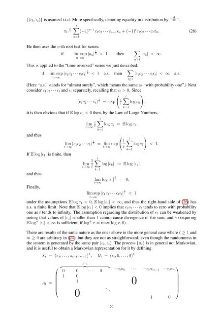
{(ct, ɛt)} is asumed i.i.d. More specifically, denoting equality in distribution by “ d = ”,
t� d
= (−1) n−1 c1c2 · · · cn−1ɛn + (−1) t c1c2 · · · ctπ0. (26)
πt
n=1
He then uses the n-th root test for series:
if lim sup |an|
n→∞
1
n < 1 then �
|an| < ∞.
This is applied to the “time-reversed” series we just described:
if lim sup |c1c2 · · · ctɛt|
t→∞
1
t < 1 a.s. then �
|c1c2 · · · ctɛt| < ∞ a.s..
(Here “a.s.” stands for “almost surely”, which means the same as “with probability one”.) Next
consider c1c2 · · · ct and ɛt separately, recalling that ct > 0. Since
(c1c2 · · · ct) 1
�
t�
�
t = exp
,
1
t
k=1
t≥1
n≥1
log ck
it is then obvious that if E log c1 < 0 then, by the Law of Large Numbers,
t�
log ck = E log c1,
and thus
If E log |ɛ1| is finite, then
and thus
Finally,
1 lim
t→∞ t
k=1
lim
t→∞ (c1c2 · · · ct) 1
t = lim exp
t→∞
1
lim
t→∞ t
�
1
t
t�
k=1
log ck
t�
log |ɛk| → E log |ɛ1|,
k=1
1
lim log |ɛt| t = 0.
t→∞
�
< 1.
lim sup |c1c2 · · · ctɛt|
t→∞
1
t < 1
under the assumptions E log c1 < 0, E log |ɛ1| < ∞, and thus the right-hand side of (26) has
a.s. a finite limit. Note that E log |c1| < 0 implies that c1c2 · · · ct tends to zero with probability
one as t tends to infinity. The assumption regarding the distribution of ɛ1 can be weakened by
noting that values of |ɛ1| smaller than 1 cannot cause divergence of the sum, and so requiring
E log + |ɛ1| < ∞ is sufficient, if log + x = max(log x, 0).
There are results of the same nature as the ones above in the more general case where ℓ ≥ 1 and
m ≥ 0 are arbitrary in (24), but they are not as straighforward, even though the randomness in
the system is generated by the same pair (ct, ɛt). The process {πt} is in general not Markovian,
and it is useful to obtain a Markovian representation for it by defining
Xt = (πt, . . . , πt−ℓ−m+1) T , Bt = (ɛt, 0, . . . , 0) T
At =
ℓ−1
⎛ � �� �
0 0 · · · 0
⎜
1 0
⎜
1
⎜
⎝
. ..
0
20
⎞
−ctα0 · · · −ctαm−1 −ctαm
⎟ 0
⎟ .
⎟
⎠
1 0