Cobweb Theorems with production lags and price forecasting

More documents

Recommendations

Info

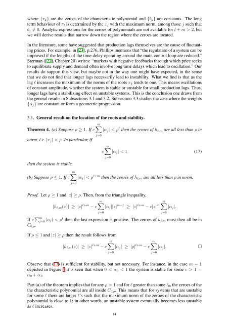
where {xk} are the zeroes of the characteristic polynomial and {bk} are constants. The long term behaviour of πt is determined by the xj with the maximum norm, among those j such that bj �= 0. Analytic expressions for the zeroes of polynomials are not available for l + m > 2, but we will derive results that narrow down the region where the zeroes are located. In the literature, some have suggested that production lags themselves are the cause of fluctuating prices. For example, in [23], p.276, Phillips mentions that “the regulation of a system can be improved if the lengths of the time delay operating around the main control loop are reduced.” Sterman ([27], Chapter 20) writes: “markets with negative feedbacks through which price seeks to equilibrate supply and demand often involve long time delays which lead to oscillation.” Our results do support this view, but maybe not in the way one might have expected, in the sense that we do not find that longer lags necessarily lead to instability. What we find is that as the lag ℓ increases the maximum of the norms of the roots xk tends to one. This means oscillations of constant amplitude, whether the system is stable or unstable for small production lags. Thus, longer lags have a stabilizing effect on unstable systems. This is the conclusion one draws from the general results in Subsections 3.1 and 3.2. Subsection 3.3 studies the case where the weights {αj} are constant or form a geometric progression. 3.1. General result on the location of the roots and stability. m� Theorem 4. (a) Suppose ρ ≥ 1. If c |αj| < ρ ℓ then the zeroes of hℓ,m are all less than ρ in norm, i.e. |xj| < ρ. In particular, if then the system is stable. (b) Suppose ρ ≤ 1. If c j=0 c m� |αj| < 1 (17) j=0 m� |αj| < ρ ℓ+m then the zeroes of hℓ,m are all less than ρ in norm. j=0 Proof. Let ρ ≥ 1 and |z| ≥ ρ. Then, from the triangle inequality, |hℓ,m(z)| ≥ |z| ℓ+m m� − c |αj||z| m−j ≥ |z| ℓ+m − c|z| m j=0 m� |αj|. If c � m j=0 |αj| < ρ ℓ then the last expression is positive. The zeroes of hℓ,m must then all be in C0,ρ. If ρ ≤ 1 and |z| ≥ ρ then the result follows from |hℓ,m(z)| ≥ |z| ℓ+m m� − c |αj| ≥ |ρ| ℓ+m − c j=0 j=0 m� |αj|. � Observe that (17) is sufficient for stability, but not necessary. For instance, in the case m = 1 depicted in Figure 4 it is seen that when 0 < α0 < 1 the system is stable for some c > 1 = α0 + α1. Part (a) of the theorem implies that for any ρ > 1 and for ℓ greater than some ℓ0, the zeroes of the the characteristic polynomial are all inside C0,ρ. This means that for systems that are unstable for some ℓ there are larger ℓ’s such that the maximum norm of the zeroes of the characteristic polynomial is close to 1; in other words, an unstable system eventually becomes less unstable as ℓ increases. 14 j=0
As an application of Theorem 4, let us now return to the cases m = 1, ℓ ≥ 1, α0 arbitrary, that we looked at in Section 2 (cf. Figure 4). Suppose ℓ is odd, and fix α0 ≥ 1. If we set c = (|α0| + |1 − α0|) −1 = 1/(2α0 − 1) then a zero of hℓ,1(x) is x = −1, and the system is unstable. However, Theorem 4 says that if c < (|α0| + |1 − α0|) −1 then the system is stable. Hence, the stability region for ℓ odd, α0 ≥ 1 consists of the points (α0, c) with c < (|α0| + |1 − α0|) −1 . The situation is similar when ℓ is even and α0 ≤ 0; then c = (|α0| + |1 − α0|) −1 = 1/(1 − 2α0) leads to a zero at x = −1 again, while Theorem 4 gives stability when c < 1/(1 − 2α0). Hence, the stability region for ℓ even, α0 ≤ 0 consists of the points (α0, c) with c < (|α0| + |1 − α0|) −1 . 3.2. Limiting behaviour with increasing production lags. The next result shows that when the production lag ℓ increases without bound, all the zeroes of the characteristic polynomial hℓ,m(x) are arbitrarily close to the unit circle, with the possible exception of up to m zeroes inside the unit circle. This means, loosely speaking, that longer production lags lead to oscillations of constant amplitude, and not to oscillations of increasing amplitude. A system that has oscillations of increasing amplitude will be made less unstable for production lags that are long enough. This partly contradicts the view that long production lags in themselves cause erratic price behaviour. We will use the following classical result from [25], page 261. Theorem (Hurwitz) Let G be a non-empty connected open set in the complex plane. Suppose φ, φn, n ≥ 1 are analytic functions on G, and that φn converges uniformly on compacts to φ in G. Let U be a bounded open set of G with U ⊂ G such that f has no zero on ∂U. Then there is an index nU ∈ N such that for each n ≥ nU the functions φ and φn have the same number of zeroes in U. Theorem 5. Define g(z) = m� αjz m−j . (18) j=0 If g has k zeroes inside the unit circle C0,1 label them r1, . . . , rk. Let ρ1 ∈ (0, 1) be such that C0,ρ1 includes r1, . . . , rk in its interior. Let ρ2 > 1. Then there exists ℓ0 < ∞ such that for any ℓ ≥ ℓ0, hℓ,m(·) has exactly the same number of zeroes in C0,ρ1 as gm and no zero outside C0,ρ2. In addition, there are sequences r1,ℓ, . . . , rk,ℓ such that • lim ℓ→∞ ri,ℓ = ri, for each 1 ≤ i ≤ k, and • For every ℓ ≥ ℓ0, hℓ,m(ri,ℓ) = g(ri) = 0. Proof. First, hℓ,m(z) converges uniformly on compact sets (in B0,1) to cg(z). Take ρ1 as defined above, and apply Hurwitz’s Theorem for G = C0,ρ1 to obtain that hℓ,m has the same number of zeroes as g inside C0,ρ1 for all ℓ ≥ ℓ0. To obtain the limiting results for each of the zeroes, apply Hurwitz Theorem to a sequence of balls around each zero ri with decreasing radius. Second, for any ρ2 > 1 there is ℓ1 such that m� c |αj| ≤ ρ ℓ 2, ℓ ≥ ℓ1, j=0 and thus by part (a) of Theorem 4 all the zeroes of hℓ,m are inside C0,ρ2 when ℓ ≥ ℓ1. � Theorem 5 explains the behaviour illustrated in Figures 6 and 9, namely that as ℓ increases, most or all the zeroes approach the boundary of the unit circle. It does not, however, explain why the zeroes are placed almost uniformly around the circle in the limit. The difference between 15
Page 1 and 2: COBWEB THEOREMS WITH PRODUCTION LAG
Page 3 and 4: Let ℓ ∈ {1, 2, . . . } be the p
Page 5 and 6: Proof. Let g(z) = m� αjz m−j ,
Page 7 and 8: 2.2. The case ℓ = 1, m = 1. Theor
Page 9 and 10: 10 8 6 4 2 2 4 6 8 10 FIGURE 5. Cri
Page 11 and 12: 3.0 2.5 2.0 1.5 1.0 0.5 0.0 ��1
Page 13: m � 3, c � 0.2, Α ��0.1, 0
Page 17 and 18: Proof. Define The characteristic po
Page 19 and 20: In order to study the effect of var
Page 21 and 22: Here At is (ℓ + m) × (ℓ + m),
Page 23 and 24: and 1 n log � |Cn| · · · |C1|
Page 25 and 26: 4.3. Numerical Experiments. In this
Page 27: [3] Bougerol, P. and Picard, N. (19

Cobweb Theorems with production lags and price forecasting

You also want an ePaper? Increase the reach of your titles

Delete template?

Save as template?