Cobweb Theorems with production lags and price forecasting

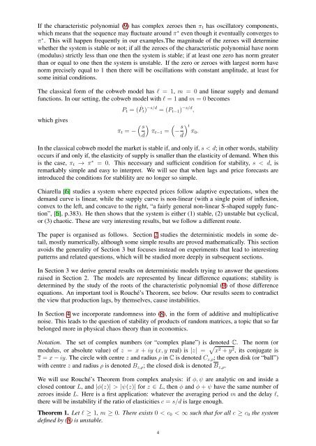
If the characteristic polynomial (9) has complex zeroes then πt has oscillatory components,
which means that the sequence may fluctuate around π ∗ even though it eventually converges to
π ∗ . This will happen frequently in our examples.The magnitude of the zeroes will determine
whether the system is stable or not; if all the zeroes of the characteristic polynomial have norm
(modulus) strictly less than one then the system is stable; if at least one zero has norm greater
than or equal to one then the system is unstable. If the zero or zeroes with largest norm have
norm precisely equal to 1 then there will be oscillations with constant amplitude, at least for
some initial conditions.
The classical form of the cobweb model has ℓ = 1, m = 0 and linear supply and demand
functions. In our setting, the cobweb model with ℓ = 1 and m = 0 becomes
which gives
Pt = ( ˆ Pt) −s/d = (Pt−1) −s/d ,
πt = −
�
s
� �
πt−1 =
d
− s
d
� t
π0.
In the classical cobweb model the market is stable if, and only if, s < d; in other words, stability
occurs if and only if, the elasticity of supply is smaller than the elasticity of demand. When this
is the case, πt → π ∗ = 0. This necessary and sufficient condition for stability, s < d, is
remarkably simple and easy to interpret. We will see that when lags and price forecasts are
introduced the conditions for stablility are no longer so simple.
Chiarella [6] studies a system where expected prices follow adaptive expectations, when the
demand curve is linear, while the supply curve is non-linear (with a single point of inflexion,
convex to the left, and concave to the right, “a fairly general non-linear S-shaped supply function”,
[6], p.383). He then shows that the system is either (1) stable, (2) unstable but cyclical,
or (3) chaotic. These are very interesting results, but we follow a different route.
The paper is organised as follows. Section 2 studies the deterministic models in some detail,
mostly numerically, although some simple results are proved mathematically. This section
avoids the generality of Section 3 but focuses instead on experiments that lead to interesting
patterns and related questions, which will be studied more deeply in subsequent sections.
In Section 3 we derive general results on deterministic models trying to answer the questions
raised in Section 2. The models are represented by linear difference equations; stability is
determined by the study of the roots of the characteristic polynomial (9) of those difference
equations. An important tool is Rouché’s Theorem, see below. Our results seem to contradict
the view that production lags, by themselves, cause instabilities.
In Section 4 we incorporate randomness into (8), in the form of additive and multiplicative
noise. This leads to the question of stability of products of random matrices, a topic that so far
belonged more in physical chaos theory than in economics.
Notation. The set of complex numbers (or “complex plane”) is denoted C. The norm (or
modulus, or absolute value) of z = x + iy (x, y real) is |z| = � x 2 + y 2 , its conjugate is
z = x − iy. The circle with centre z and radius ρ in C is denoted Cz,ρ; the open disk (or “ball”)
with centre z and radius ρ is denoted Bz,ρ; the closed disk is denoted Bz,ρ.
We will use Rouché’s Theorem from complex analysis: if φ, ψ are analytic on and inside a
closed contour L, and |φ(z)| > |ψ(z)| for z ∈ L, then φ and φ + ψ have the same number of
zeroes inside L. Here is a first application: whatever the averaging period m and the delay ℓ,
there will be instability if the ratio of elasticities c = s/d is large enough.
Theorem 1. Let ℓ ≥ 1, m ≥ 0. There exists 0 < c0 < ∞ such that for all c ≥ c0 the system
defined by (8) is unstable.
4