arXiv:1602.08159v2

Harnessing disordered ensemble quantum dynamics for machine learning
arXiv:1602.08159v2 [quant-ph] 9 Nov 2016
Keisuke Fujii 1, 2, 3, 4 2, 4, 5
and Kohei Nakajima
1 Photon Science Center, Graduate School of Engineering,
The University of Tokyo, 2-11-16 Yayoi, Bunkyo-ku, Tokyo 113-8656, Japan
2 The Hakubi Center for Advanced Research, Kyoto University,
Yoshida-Ushinomiya-cho, Sakyo-ku, Kyoto 606-8302, Japan
3 Department of Physics, Graduate School of Science, Kyoto University,
Kitashirakawa Oiwake-cho, Sakyo-ku, Kyoto 606-8502, Japan
4 JST, PRESTO, 4-1-8 Honcho, Kawaguchi, Saitama 332-0012, Japan
5 Graduate School of Informatics, Kyoto University,
Yoshida Honmachi, Sakyo-ku, Kyoto 606-8501, Japan
(Dated: November 10, 2016)
Quantum computer has an amazing potential of fast information processing. However, realisation
of a digital quantum computer is still a challenging problem requiring highly accurate controls and
key application strategies. Here we propose a novel platform, quantum reservoir computing, to solve
these issues successfully by exploiting natural quantum dynamics of ensemble systems, which is ubiquitous
in laboratories nowadays, for machine learning. This framework enables ensemble quantum
systems to universally emulate nonlinear dynamical systems including classical chaos. A number of
numerical experiments show that quantum systems consisting of 5–7 qubits possess computational
capabilities comparable to conventional recurrent neural networks of 100–500 nodes. This discovery
opens up a new paradigm for information processing with artificial intelligence powered by quantum
physics.
I. INTRODUCTION
Quantum physics, which is the fundamental framework
of physics, exhibits rich dynamics, sufficient to explain
natural phenomena in microscopic worlds. As Feynman
pointed out [1], the simulation of quantum systems on
classical computers is extremely challenging because of
the high complexity of these systems. Instead, they
should be simulated by using a machine of which the
operation is based on the laws of quantum physics.
Motivated by the recent rapid experimental progress in
controlling complex quantum systems, non-conventional
information processing utilising quantum physics has
been explored in the field of quantum information science
[2, 3]. For example, certain mathematical problems,
such as integer factorisation, which are believed to
be intractable on a classical computer, are known to be
efficiently solvable by a sophisticatedly synthesized quantum
algorithm [4]. Therefore, considerable experimental
effort has been devoted to realising full-fledged universal
quantum computers [5, 6]. On the other hand, quantum
simulators are thought to be much easier to implement
than a full-fledged universal quantum computer. In this
regard, existing quantum simulators have already shed
new light on the physics of complex many-body quantum
systems [7–9], and a restricted class of quantum
dynamics, known as adiabatic dynamics, has also been
applied to combinatorial optimisation problems [10–13].
However, complex real-time quantum dynamics, which
is one of the most difficult tasks for classical computers
to simulate [14–16] and has great potential to perform
nontrivial information processing, is now waiting to be
harnessed as a resource for more general purpose information
processing. Specifically, the recent rapid progress
in sensing and Internet technologies has resulted in an increasing
demand for fast intelligent big data analysis with
low energy consumption. This has motivated us to develop
brain-inspired information processing devices of a
non-von Neumann type, on which machine learning tasks
are able to run natively [17].
Here we propose a novel framework to exploit the complexity
of real-time quantum dynamics in ensemble quantum
systems for nonlinear and temporal learning problems.
These problems include a variety of real-world
tasks such as time-dependent signal processing, speech
recognition, natural language processing, sequential motor
control of robots, and stock market predictions. Our
approach is based on a machine learning technique inspired
by the way the brain processes information, socalled
reservoir computing [18–20]. In particular, this
framework focuses on real-time computing with timevarying
input that requires the use of memory, unlike
feedforward neural networks. In this framework, the lowdimensional
input is projected to a high-dimensional dynamical
system, which is typically referred to as a reservoir,
generating transient dynamics that facilitates the
separation of input states [21]. If the dynamics of the
reservoir involve both adequate memory and nonlinearity
[22], emulating nonlinear dynamical systems only requires
adding a linear and static readout from the highdimensional
state space of the reservoir.
A number of different implementations of reservoirs
have been proposed, such as abstract dynamical systems
for echo state networks (ESNs) [18] or models of neurons
for liquid state machines [19]. The implementations are
not limited to programs running on the PC but also include
physical systems, such as the surface of water in a
laminar state [23], analogue circuits and optoelectronic

2
systems [24–29], and neuromorphic chips [30]. Recently,
it has been reported that the mechanical bodies of soft
and compliant robots have also been successfully used
as a reservoir [31–36]. In contrast to the refinements
required by learning algorithms, such as in deep learning
[37], the approach followed by reservoir computing,
especially when applied to real systems, is to find an appropriate
form of physics that exhibits rich dynamics,
thereby allowing us to outsource a part of the computation.
Nevertheless, no quantum physical system has been
employed yet as a physical reservoir.
Here we formulate quantum reservoir computing
(QRC) and show, through a number of numerical experiments,
that disordered quantum dynamics can be used
as a powerful reservoir. Although there have been several
prominent proposals on utilising quantum physics in
the context of machine learning [38–43], they are based
on sophisticatedly synthesised quantum circuits on a fullfledged
universal quantum computer. Contrary to these
software approaches, the approach followed by QRC is
to exploit the complexity of natural (disordered) quantum
dynamics for information processing, as it is. Here
disordered quantum dynamics means that couplings are
random, and hence no fine tuning of the parameters of
the Hamiltonian is required. Any quantum chaotic (nonintegrable)
system can be harnessed, and its computational
capabilities are specified. This is a great advantage,
because we can utilise existing quantum simulators
or complex quantum systems as resources to boost information
processing. Among existing works on quantum
machine learning [38–41, 43], our approach is the first attempt
to exploit quantum systems for temporal machine
learning tasks, which essentially require a memory effect
to the system. As we will see below, our benchmark results
show that quantum systems consisting of 5–7 qubits
already exhibit a powerful performance comparable to
the ESNs of 100-500 nodes. Not only its computational
power, QRC will also provide us an operational means to
approach complex real-time quantum dynamics. While
there had been a missing operational link between classical
chaos and quantum chaotic systems manifested by
a Wigner-Dyson type statistics of the energy level spacing
[44, 45], it is quite natural to connect them via the
QRC framework naturally as an emulation of classical
chaos by quantum chaotic systems. Moreover, since complex
quantum dynamics is ubiquitous, this framework
provides us new operational understanding of quantum
physics, such as quantum simulation, thermodynamics in
closed quantum system and fast scrambling in black hole.
(a)
(b)
reservoir computing
input
quantum reservoir computing
input
input
Sk
1 Input
0.8
0.6
0.4
0.2
0
hidden nodes
quantum system
true nodes
virtual
nodes
}
LR
signal
x’i (t )
LR
output
output
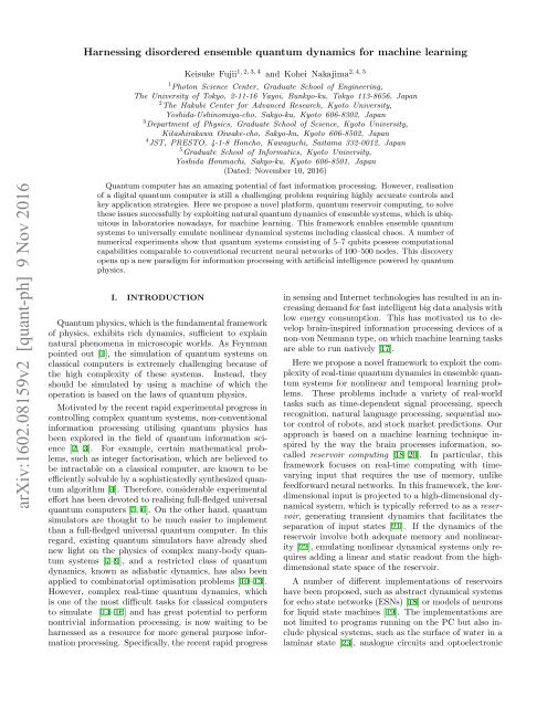
FIG. 1. Information processing scheme in QRC. (a) The
input sequence {s k } is injected into the quantum system.
The signal x ′ i(t) is obtained from each qubit. (b) Comparison
between conventional (upper) and quantum (lower) reservoir
computing approaches. Note that the circles in the QRC do
not represent qubits, but the basis of the Hilbert space like
the nodes in quantum walk [39, 46, 47]. The true nodes correspond
to a subset of basis of the operator space that are
directly monitored by the ensemble measurements. The hidden
nodes correspond to the remaining degrees of freedom.
unit of information in quantum physics is a quantum bit
(qubit), which consists of a two-level quantum system,
namely a vector in a two-dimensional complex vector
space of spanned by {|0〉, |1〉}. Let us consider a quantum
system consisting of N qubits, which is described
as a tensor product space of a complex vector space of
two dimensions. A pure quantum state is represented
by a state vector |ψ〉 in a 2 N -dimensional complex vector
space. We may also consider a statistical (classical)
mixture of the states of the pure states, which can be
described by a 2 N × 2 N hermitian matrix ρ known as a
density matrix. For a closed quantum system, the time
evolution for a time interval τ is given by a unitary operator
e −iHτ generated by a hermitian operator H called
Hamiltonian. Specifically, for the density matrix the time
evolution is given by
II.
QUANTUM RESERVOIR COMPUTING
A. Description of quantum system and dynamics
ρ(t + τ) = e −iHτ ρ(t)e iHτ , (1)
In this subsection, we will explain how to describe
quantum system and dynamics for the readers who are
not familiar with quantum information. The minimum
where the Hamiltonian H is an 2 N ×2 N hermitian matrix
and defines the dynamics of the quantum system.

3
B. Measurements in ensemble quantum systems
Measurements in quantum system is described by a set
of projective operators {P i }, which satisfies ∑ i P i = I
and P i P j = δ ij P i . Then the probability to obtain
the measurement outcome i for the state ρ is given by
p i = Tr[P i ρ]. The state after the measurement gets a
backaction and is given by P i ρP i /Tr[P i ρ]. That is, a single
quantum system inevitably disturbed by the projective
measurement. By repeating the projective measurements,
we can calculate average values 〈O〉 := Tr[Oρ] of
an observable O = ∑ i a iP i .
Here we consider an ensemble quantum system, where
the system consists of a huge number of the copies of
ρ, i.e., ρ ⊗m . Cold atomic ensembles and liquid or solid
state molecules are natural candidates of such an ensemble
quantum system. For example, in an NMR (nuclear
magnetic resonance) spin ensemble system, we have typically
10 18−20 copies of the same molecules [48, 49]. Nuclear
spin degree of freedoms of them can be employed as
the quantum system, like NMR spin ensemble quantum
computers or synthetic dimensions of ultra cold atoms
for quantum simulations. We here assume that we can
obtain the signals as a macroscopic observable from the
ensemble quantum system directly, where the ensemble
quantum system and the probe system are coupled by an
extremely weak interaction. Actually, the NMR bulk ensemble
average measurement is done in this way. There
is almost no backaction, or backaction is much smaller
than other imperfections like the T 1 relaxation [48, 49].
In QRC, we make an active use of such a property of
the ensemble quantum systems to exploit the complex
quantum dynamics on the large degrees of freedom.
C. Definition of quantum reservoir dynamics
As nodes of the network of the QR, we use an orthogonal
basis of quantum states. The idea is similar to the
quantum walks [39, 46, 47], where each individual node
is defined not by qubits (subsystems) but by basis states
like {|000〉, |001〉, ..., |111〉}. Therefore, for N qubits, we
have 2 N basis states for a pure quantum state. Moreover,
here we employ the density matrix in general, we
define the nodes of the network by an orthogonal basis of
the operator space of the density matrices. By using the
Hilbert-Schmidt inner product, the density matrix can
be represented as a vector x on a 4 N -dimensional operator
space. Here the i-th coefficient x i of x is defined
by x i = Tr[B i ρ] by using the set of N-qubit products
of the Pauli operators {B i } 4N
i=1 = {I, X, Y, Z}⊗N (where
B i B j = δ ij I). Specifically, we choose the first N elements
such that B i = Z i for convenience in the definition of the
observables later.
In this operator space, the time evolution is reformulated
as a linear map for the vector x:
x(t + τ) = U τ x(t). (2)
Here U τ is a 4 N × 4 N matrix whose element is defined by
(U τ ) ji := Tr[B j e −iHτ B i e iHτ ]. (3)
Owing to the unitarity of the dynamics e −iHτ (e −iHτ ) † =
I, we have U τ U T τ = I. If the system is coupled to an external
system for a measurement and/or a feedback operation,
the time evolution (for the density matrix) is not
given by the conjugation of the unitary operator e −iHτ ;
instead, it is generally given by a complete positive trace
preserving (CPTP) map D for the density matrix ρ. Even
in such a case, the dynamics is linear, and hence the time
evolution for x(t) is given in a linear form:
where the matrix element is defined
x → W x (4)
W ji := Tr[B j D(B i )]. (5)
In order to exploit quantum dynamics for information
processing, we have to introduce an input and the signals
of the quantum system (see Fig. 1 (a)). Suppose
{s k } M k=1 is an input sequence, where s k can be a binary
(s k ∈ {0, 1}) or a continuous variable (s k ∈ [0, 1]). A
temporal learning task here is to find, using the quantum
system, a nonlinear function y k = f({s l } k l=1
) such that
the mean square error between y k and a target (teacher)
output ȳ k for a given task becomes minimum. To do
so, at each time t = kτ, the input signal s k is injected
into a qubit, say the 1st qubit, by replacing (or by using
measurement and feedback) the 1st qubit with the state
ρ sk = |ψ sk 〉〈ψ sk |, where
|ψ sk 〉 := √ 1 − s k |0〉 + √ s k |1〉. (6)
The density matrix ρ of the system is transformed by the
following CPTP map:
ρ → ρ sk ⊗ Tr 1 [ρ], (7)
where Tr 1 indicates the partial trace with respect to the
first qubit. The above action of the kth input on the
state x(t) is again rewritten by a matrix S k by using
Eq. (5). After the injection, the system evolves under
the Hamiltonian H for a time interval τ. Thus, the time
evolution of the state for a unit timestep is given by
x(kτ) = U τ S k x ((k − 1)τ) . (8)
After injecting the kth input, the system evolves under
the Hamiltonian for τ time. The time interval τ should
be determined by both physical constraint for the input
injections and performance of the QR.
The signal, which is exploited for the learning process,
is defined as an average value of a local observable on each
qubit. We here employ, as observables, the Pauli operator
Z i acting on each ith qubit. For an appropriately ordered
basis {B i } in the operator space, the observed signals,
and the first N elements of the state x(t) are related by
x i (t) = Tr[Z i ρ(t)] (i = 1, ..., N). As we mentioned before,
we do not consider the backaction of the measurements

4
p
1 s1|0i + p s 1|1i
p
1 s2|0i + p s 2|1i
|0ih0| ⌦ I + |1ih1| ⌦ X
p
1 s1|0i + p s 1|1i
e iH⌧
p
1 s2|0i + p s 2|1i
e iH⌧
hZ out i =
(1 2s 1 )(1 2s 2 )
FIG. 2. Physical insight of QRC. (top) A quantum circuit
whose output has the second order nonlinearity with respect
to the input variables s 1 and s 2. (bottom) The quantum
circuit is replaced by a unitary time evolution under a Hamiltonian
H. The observables are monitored by the ensemble
average measurements.
to obtain the average values {x i (t)} by considering an
ensemble quantum system. We call the directly observed
signals {x i (t)} N i=1 as the true nodes. Then, the remaining
(4 N − N) nodes of x(t) as hidden nodes, as they are not
employed as the signals for learning. For the learning,
we employ x ′ i (t) defined by
x ′ i(t) := Tr[(I + Z i )/2ρ(t)] = (x i (t) + 1)/2 (9)
by adding a constant bias and rescaling with 1/2 just for
a convenience for the presentation.
The unique feature of QRC in the reservoir computing
context is that the exponentially many hidden nodes
originated from the exponentially large dimensions of the
Hilbert space are monitored from a polynomial number of
the signals defined as the true nodes as shown in Fig. 1
(b). Contrast to a single quantum system, the ensemble
quantum system allows us to make real-time use of
the exponentially large degrees of freedom. Note that at
the injected one clean qubit at each time step and the
single-qubit averaged outputs after a unitary time evolution
is enough hard for a classical computer to simulate
efficiently in general [14, 15].
D. Emerging nonlinearity from a linear system
We here provide a physical insight why quantum disordered
dynamics can be employed for nonlinear learning
task. One might think that the quantum system is totally
linear, and hence that we cannot employ it for learning
tasks, which essentially require nonlinearity. However,
this is not the case. The definition of the nonlinearity
defined for the learning task and the linearity of the dynamics
on the quantum system are quite different. Let
us, for example, consider a quantum circuit shown in
Fig. 2. For two input states |ψ s1 〉 = √ 1 − s 1 |0〉 + √ s 1 |1〉
and |ψ s2 〉 = √ 1 − s 2 |0〉 + √ s 2 |1〉, we obtain 〈Z out 〉 =
(1 − 2s 1 )(1 − 2s 2 ), which has the second order nonlinearity
with respect to s 1 and s 2 . Or equivalently, in the
Heisenberg picture, the observable Z out corresponds to
the nonlinear observable Z 1 Z 2 . Whereas dynamics is described
as a linear map, information with respect to any
kind of correlation exists in exponentially many degrees
of freedom. In the QRC, such higher order correlations
or nonlinear terms are mixed by the linear but quantum
chaotic (non-integrable) dynamics U τ . There exists
a state corresponding to an observable B l = Z i Z j ,
i.e. x l (t) = Tr[Z i Z j ρ(t)] storing correlation between
x i (t) = Tr[Z i ρ(t)] and x j (t) = Tr[Z j ρ(t)], which can be
monitored from another true node via U τ . This mechanism
allows us to find a nonlinear dynamics with respect
to the input sequence {s k } from the dynamics of
the true nodes {x i (t)} N i=1 . The emergent nonlinearlity
is not as special because classical (nonlinear) dynamics
appears as (coarse-grained) dynamics of averaged values
of the observables in the quantum system. However, the
universal emulation of nonlinear dynamics by training an
optimal observable in disordered (chaotic) quantum systems
explained below is unique for QRC, providing an
alternative paradigm to digital universal quantum computing.
E. Training readout weights
Here we explain how to train the QR from the observed
signals. We harness complex quantum dynamics
in a physically natural system by utilizing the reservoir
computing approach. Here the signals are sampled
from the QR not only at the time kτ, but also at each
of the subdivided V timesteps during the unitary evolution
U τ as shown in Fig. 3. That is, at each time
t + v(τ/V ) with an integer 1 ≤ v ≤ V , the signals
x ′ i (t+v(τ/V )) = Tr[Z iρ(t+v(τ/V ))] are sampled. Thus,
at each timestep k, we have NV virtual nodes in total.
These time multiplexed signals are denoted by x ′ ki with
i = n + vN with integers 1 ≤ n ≤ N and 0 ≤ v ≤ V ,
x ′ ki
, which means the signal of the nth qubit at time
t = kτ + v(τ/V ), i.e. x ′ ki := x′ i (kτ + v(τ/V )). We have
named these virtual nodes (a similar technique of time
multiplexing is also used in e.g. Ref. [24]). The virtual
nodes allow us to make full use of the richness of quantum
dynamics, because unitary real-time evolution is essential
for nonlinearity.
Suppose learning is performed by using L timesteps.
Let {x ′ ki
} (1 ≤ i ≤ NV and 1 ≤ k ≤ L) be the states
of the virtual nodes in the learning phase. We also introduce
x ′ k0 = 1.0 as a constant bias term. Let {ȳ k} L k=1

1
0.8
0.6
x’i (t )
0.4
0.8
0.6
0.4
0.2
0.2
1
0
quantum dynamics
0
1000 1050 1100 1150 time t 1200
…
1060 1062 1064 1066 τ1068
1070 1072
qubit 1
time
multiplexing
2
3
4
5
virtual node x’i (t )
…
…
…
…
…
}
# of virtual nodes V
output
readout
FIG. 3. Quantum reservoir dynamics and virtual nodes. The
time interval τ is divided into V subdivided timesteps. At
each subdivided timestep the signals are sampled. Using the
NV signals as the virtual nodes for each timestep k in the
learning phase, the linear readout weights {wi
LR } are trained
for a task.
Using w LR , we obtain the output from the QR
5
∑NV
y k = wi LR x ′ ki. (14)
i=0
Or equivalently, an optimal observable
O trained ≡
N∑
i=1
wi
LR (I + Z i )/2 + wN+1I LR (15)
is trained, and the output is obtained as 〈O trained 〉.
Specifically, as is the case in the conventional reservoir
computing approach, none of the parameters of the
system (Hamiltonian) requires fine tuning except for the
linear readout weights. Thus, we can employ any quantum
system (Hamiltonian) as long as it exhibits dynamics
with appropriate properties for our purpose, such as
fading memory and nonlinearity. That is, as long as the
QR is sufficiently rich, we can find an optimal observable
O trained capable of exploiting the preferred behaviour via
the training (learning) process. In the following numerical
experiments, we employ, as an example, the simplest
quantum system, a fully connected transverse-field Ising
model, which exhibits a Wigner-Dyson statistics of the
energy level spacing [44, 45, 50]:
H = ∑ ij
J ij X i X j + hZ i , (16)
be the target sequence for the learning. In the reservoir
computing approach, learning of a nonlinear function
y m = f({s k } m k=1
), which emulates the target sequence
{ȳ k }, is executed by training the linear readout weights
of the reservoir states such that the mean square error
1
L
L∑
(y k − ȳ k ) 2 (10)
k=1
is minimised. That is, what we have to do is to find linear
readout weights {w i } NV
i=0 to obtain the output sequence
∑NV
y k = x ′ kiw i (11)
i=0
with the minimum mean square error. This problem corresponds
to solving the following equations:
ȳ = Xw, (12)
where {x ′ ki }, {ȳ k} L k=1 , and {w i} NV
i=0 are denoted by a
L × (NV + 1)matrix X, and column vectors ȳ and w, respectively.
Here we assume that the length of the training
sequence L is much larger than the total number of the
nodes NV + 1 including the bias term. Thus, the above
equations are overdetermined, and hence the weights
that minimise the mean square error are determined by
the Moore-Penrose pseudo-inverse X + := (X T X) −1 X T
((NV + 1) × L matrix) of X as follows:
w LR := X + ȳ. (13)
where the coupling strengths are randomly chosen such
that J ij is distributed randomly from −J/2 to J/2. We
introduce a scale factor ∆ so as to make τ∆ and J/∆ dimensionless.
Note that we do not employ any approximation,
but quantum dynamics of the above Hamiltonian is
exactly calculated to evaluate the potential performance
of the QRs. The imperfections including decoherence and
noise on the observed signals, which might occur in actual
experiments, are further taken into account in Sec. IV B.
III.
DEMONSTRATIONS OF QRC FOR
TEMPORAL LEARNING TASKS
We start by providing several demonstrations to obtain
a sense of QRC using a number of benchmark tasks in
the context of machine learning.
A. Timer task
Our first experiment is to construct a timer. One important
property of QRC is having memory to be exploited.
Whether the system contains memory or not
can be straightforwardly evaluated by performing this
timer task (see e.g., [51]). The input is flipped from 0
to 1 at certain timestep (k ′ ) as a cue, and the system
should output 1 if τ timer timesteps have passed from the
cue, otherwise it should output 0 (see Fig.4 (a), left diagram).
To perform this task, the system has to be able to

6
s k
y k y k y k y k y k
(a)
(b)
0.20
0.10
0
0.20
0.196
0.192
0.22
0.18
0.22
0.18
0.24
0.20
0.28
(timer task)
1
0
k’ timestep k’
input (s k ) output (y k )
QR
target
system (V=1)
system (V=2)
τ
timer
timestep
system (V=5)
system (V=10)
NARMA2
NARMA5
NARMA10
NARMA15
NARMA20
s k
y k
y k
y k
y k
y k
y k
y k
1 input
0
1 τ
0
1 τ
0
1 τ
0
1 τ
timer=5
timer=10
timer=15
timer=20
timer=25
timer=30
0
490 500 510 520
timestep
530 540
( τ MG =16)
1
0
1
0 1 0 1 0 1
target
case1
case2
0
10000 10200 10400 10600 10800 11000
timestep
( τ MG =17)
1
target
case1
case2
case3
0
1
0 1
case4
0.24
0
4000 4100 4200 4300 10000 10200 10400 10600 10800 11000
timestep
timestep
target
system (V=2)
system (V=1) system (V=10)
(c)
0
1
y k
0
1 0 1
FIG. 4. Typical performances of QR for temporal machine learning tasks. (a) The timer task. A 6-qubit QR system is prepared,
and starting from different initial conditions, 10 trials of numerical experiments were run for each τ timer setting. k ′ is set to
500 throughout the numerical experiments. The plots overlay the averaged system performance over 10 trials for V = 1, 2, 5,
and 10 with the target outputs. (b) The NARMA emulation task. This task requires five different NARMA systems driven
by a common input stream to be emulated. The upper plot shows the input stream, and the corresponding task performances
of a 6-qubit QR system for five NARMA tasks are plotted, overlaying the case for each V with the target outputs. (c) The
Mackey-Glass prediction task. The performances for τ MG = 16 (non-chaotic) and 17 (chaotic) are shown. The trained system
outputs are switched to the autonomous phase at timestep 10000. Two-dimensional plots, (y k , y k+15 ), are depicted for the
autonomous phase in each case. For each setting of τ MG, case 1 represents the case for 6 qubits, otherwise represent the cases
for 7 qubits. For all tasks, the detailed settings and analyses are provided in Appendix.
0
1 τ
0
1 τ
y k+15
y k

7
‘recognize’ the duration of time that has passed since the
cue was launched. This clearly requires memory. Here
we used 6-qubit QRs with τ∆ = 1 to perform this task
by incrementally varying V .
Figure 4 (a) shows the task performance with trained
readouts. We can clearly observe that by increasing V
the performance improved, which means that the amount
of memory, which can be exploited, also increased. In
particular, when V = 5 and 10, the system outputs
overlap with the target outputs within the certain delay,
which clearly demonstrates that our QR system is
capable of embedding a timer. By increasing the delay
timesteps τ timer , we can gradually see that the performance
declines, which expresses the limitation of the
amount of memory that can be exploited within the QR
dynamics. It is interesting to note that while the systems
are highly disordered, we can find an observable O trained
or a mode, at which the wave function of the system is focused
after a desired delay time τ timer . This is very useful
as a control scheme for engineering quantum many-body
dynamics. For further information, see detailed settings,
experimental and learning procedures, and analyses for
the timer task in Appendix A 1.
B. NARMA task
The second task is the emulation of nonlinear dynamical
systems, called nonlinear auto-regressive moving average
(NARMA) systems, which is a standard benchmark
task in the context of recurrent neural network learning.
This task presents a challenging problem for any computational
system because of its nonlinearity and dependence
on long time lags [52]. The first NARMA system is
the following second-order nonlinear dynamical system:
y k+1 = 0.4y k + 0.4y k y k−1 + 0.6s 3 k + 0.1. (17)
This system was introduced in Ref. [53] and used, for
example, in Refs. [33, 35]. For descriptive purposes, we
call this system NARMA2. The second NARMA system
is the following nonlinear dynamical system that has an
order of n:
n−1
∑
y k+1 = αy k + βy k ( y k−j ) + γs k−n+1 s k + δ, (18)
j=0
where (α, β, γ, δ) are set to (0.3, 0.05, 1.5, 0.1), respectively.
Here, n is varied using the values of 5, 10, 15, and
20, and the corresponding systems are called NARMA5,
NARMA10, NARMA15, and NARMA20, respectively.
In particular, NARMA10 with this parameter setting
was introduced in Ref. [53] and broadly used (see, e.g.,
Refs. [20, 33, 35]). As a demonstration, the input s k
is expressed as a product of three sinusoidal functions
with different frequencies. (Note that when the input is
projected to the first qubit, the value is linearly scaled to
[0, 1]; see Appendix A 2 for details). Here, according to an
input stream expressed as a product of three sinusoidal
functions with different frequencies, the system should simultaneously
emulate five NARMA systems (NARMA2,
NARMA5, NARMA10, NARMA15, and NARMA20),
which we call multitasking.
Figure 4 (b) plots the input sequence and the corresponding
task performance of our 6-qubit QR system
with τ∆ = 1 with trained readout by varying V . We can
clearly observe that by increasing V , the performance
improves, so that when V = 10, the system outputs almost
overlap with the target outputs. Further information
and extended analyses on the tasks with random
input streams can be found in Appendix A 2.
C. Mackey-Glass prediction task
The third experiment is a Mackey-Glass (MG) time series
prediction task, including a chaotic time series. This
is also a popular benchmark task in machine learning
(e.g., [18]). Here, unlike the previous two cases, the system
output is fed back as the input for the next timestep,
which means that when the system with trained readout
generates outputs, it receives its own output signals
through the feedback connections instead of through external
inputs. To train the readout weights, the system is
forced by the correct teacher output during presentation
of the training data, without closing the loop. A slight
amount of white noise is added to the reservoir states in
the training phase to make the trained system robust,
and the weights are trained through the usual procedure
(see Appendix A 3 for further information). The MG system
has a delay term τ MG , and when τ MG > 16.8 it exhibits
a chaotic attractor. We first test a non-chaotic case
(τ MG = 16) for comparisons and then test the chaotic
case, where τ MG = 17, which is the standard value employed
in most of the MG system prediction literature.
Figure 4 (c) depicts the typical task performances of
6- and 7-qubit QR systems. When τ MG = 16, the system
outputs overlap the target outputs, which implies
successful emulations. When τ MG = 17, our systems
tend to remain relatively stable in the desired trajectory
for about 200 steps, after switched from teacher
forced condition, start to deviate perceptibly large. Furthermore,
checking a two-dimensional plot by plotting
points (y k , y k+15 ), it appears that the learned model has
captured the essential structure of the original attractor
(e.g., when τ MG = 17, the model actually demonstrates
chaos). In both tasks, the 7-qubit QR systems generally
performed better than the 6-qubit QR systems. Further
details can be found in Appendix A 3.
IV.
PERFORMANCE ANALYSES
We perform detailed analyses on the computational capabilities
of the 5-qubit QRs focusing on the two popular
benchmark tasks of Boolean function emulations over a

8
(a)
CSTM(τB)
(b)
CPC(τB)
1
0.8
0.6
0.4
0.2
LR
V=1
V=2
V=5
V=10
V=25
V=50
0
0 10 20 30 40 50
1
0.8
0.6
0.4
0.2
delay τB
0
1 2 3 4 5 6 7 8 9 10
delay τB
LR
VV=1
VV=2
VV=5
VV=10
VV=25
VV=50
V: # of virtual nodes
V: # of virtual nodes
50
45
40
35
30
25
20
15
10
5
50
45
40
35
30
25
20
15
10
5
20
15 10
CSTM
22
20
18
16
14
12
10
8
6
4
2
0
1 10
τΔ
100
CPC
7
2
1
3
4
1 10 100
τΔ
5
5
6
6
5
4
3
2
1
0
CPC CSTM
30
25
20
15
10
5
0
4
3.5
3
2.5
2
1.5
1
0.5
0
J/Δ=1.0 J=1.0xx
J/Δ=0.5 J=0.5xx
J/Δ=0.2 J=0.2xx
J/Δ J/Δ=0.1
J/Δ=0.05
J=0.1xx
J/Δ J=0.05xx
J/Δ=1.0 J=1.0xx
J/Δ=0.5 J=0.5xx
J/Δ=0.2 J=0.2xx
J/Δ=0.1 J=0.1xx
J/Δ
J/Δ=0.05
J=0.05xx
1 10 100
τΔ
1 10 100
τΔ
FIG. 5. Performance analyses of the 5-qubit QRs. (a) (left) STM curve C STM(τ B) plotted as a function of the delay τ B for
J/∆ = 2h/∆ = 1, τ∆ = 1 and V = 1–50. (middle) STM capacity C STM plotted as a function of the number of virtual
nodes V with the same QR settings for τ∆ = 0.5–128. (right) STM capacity C STM plotted as a function of τ∆ with couplings
J/∆ = 0.05–1.0 and h/∆ = 0.5. (b) PC curve C PC(τ B) and capacity C PC plotted with the same settings as (a). The error bars
in the left and right panels indicate the standard deviations of the capacities evaluated on 20 samples of the QRs with respect
to the random couplings.
binary input sequence (see e.g., Refs. [34, 54]), which
we name the short-term memory (STM) task and parity
check (PC) task. The former task is intended to emulate
a function that outputs a version of the input stream
delayed by τ B timesteps, whereas the latter is intended
to emulate an τ B -bit parity checker. Both tasks require
memory to be emulated, and the PC task requires nonlinearity
in addition, because the parity checker function
performs nonlinear mapping. Hence, the STM task can
evaluate the memory capacity of systems and the PC
task can additionally evaluate the amount of nonlinearity
within systems.
The function for the STM task can be expressed as
follows:
y k = s k−τB ,
where s k is a binary sequence and τ B represents the delay.
The function for the PC task is expressed as follows:
y k = Q(
Q(x) =
τ B
∑
m=0
s k−m ),
{
0 (x ≡ 0 (mod 2))
1 (otherwise).
We investigated both tasks thoroughly by applying a
random input sequence for the tasks such that there
is no external source to provide temporal coherence to
the system. In these tasks, one trial consists of 5000
timesteps. The first 1000 timesteps are discarded, the
next 3000 timesteps are used for training, and the last
1000 timesteps are used for system evaluation. We evaluated
the system performance with the target output for
each given τ B by using the measure known as τ B -delay
capacity C(τ B ) expressed as
C(τ B ) = cov2 (y k , ȳ k )
σ 2 (y k )σ 2 (ȳ k ) .
In the main text, τ B -delay capacities for the STM task
and the PC task are termed τ B -delay STM capacity
C ST M (τ B ) and τ B -delay PC capacity C P C (τ B ), respectively.
Note that, in the analyses, to reduce a bias due
to the effect of the finite data length, we have subtracted
C(τB
max)
from C(τ B), where τB
max is a substantially long
delay. The capacity C is defined as
C =
τB∑
max
τ B =0
C(τ B ),
where τB
max was 500 throughout our experiments. The
capacities for the STM task and the PC task are referred
to as the STM capacity C ST M and the PC capacity C P C ,
respectively. For each task, 20 samples of the QRs were
randomly generated, and the average values of the τ B -
delay capacities and the capacities were obtained.
In Fig. 5 (a) (left), C STM (τ B ) is plotted as a function
of τ B for V = 1, ..., 50, where τ∆ = 1 and J/∆ = 1.0 are

9
Short term memory
capacity CSTM
35
30
25
20
15
10
5
1D transverse
Ising QR
0
1 10
virtual node V
4
tau=1
tau=23.5
tau=4
tau=8 3
tau=16
tau=322.5
tau=64
2
Parity check capacity CPC
1.5
1
0.5
1D transverse
Ising QR
0
1 10
virtual node V
tau=1
tau=2
tau=4
tau=8
tau=16
tau=32
tau=64
FIG. 6. STM (left) and PC (right) capacities for the 1D
transversal Ising model. The error bars show the standard
deviations evaluated on 20 samples of the QRs with respect
to the random couplings
set. The abrupt decay exhibited by the curve is improved
when the number of virtual nodes is increased. In Fig. 5
(a) (middle), the STM capacity is plotted as a function
of the number of virtual nodes V and the time interval
τ∆. It shows that the STM capacity becomes saturated
around V = 10. The 5-qubit QRs with τ∆ = 0.5 and 1.0
exhibit a substantially high STM capacity ∼ 20, which
is much higher than that of the ESNs of 500 nodes (see
Sec. IV A for details). A plot of the STM capacity as a
function of τ for a fixed number of virtual nodes V = 10
does not exhibit monotonic behaviour as shown in Fig. 5
(right). This behaviour is understood as follows. In the
limit of τ → 0, the dynamics approach an identity map
and hence become less attractive, and this is more desirable
to maintain the separation among different inputs.
At the same time, a shorter τ implies less information
is embedded in the present input setting. In the limit
of larger τ, on the other hand, the input sequence is injected
effectively; however, the dynamics become attractive,
and the separation fades rapidly. Originating from
these two competing effects, there is an optimal time interval
τ for which the STM capacity is maximised.
In Fig. 5 (b) (left), C PC (τ B ) is plotted as a function
of τ B for V = 1, ..., 50. Specifically, C PC (τ B ) is exactly
zero when V = 1. This clearly shows that the virtual
nodes, which spatialize the real-time dynamics during the
interval τ, are important to extract nonlinearity. In Fig. 5
(b) (middle), the PC capacity is plotted as a function of
the number of virtual nodes V and the time interval τ∆.
As expected, the longer the time interval τ is, the higher
the PC capacity exhibited by the QR, as shown in Fig. 5
(middle and right). This is because the true nodes are
able to increase communication with the virtual nodes.
The number of virtual nodes required for the saturation
of the PC capacity is also increased in the case of a longer
τ.
A. Characterizations of QRs
Let us clarify the unique properties of the QRs in terms
of the STM and PC capacities. We plot (C STM , C PC ) for
the 5-qubit QRs with various coupling settings in Fig. 7
(a), which include a restricted type of QR with onedimensional
nearest-neighbour (1DNN) couplings, i.e.
J ij ≠ 0 only for j = i + 1 in Eq. (16). In this case, the
transversal-field Ising model becomes integrable, that is,
exactly solvable by mapping it into a free-fermionic model
via the Jordan-Wigner transformation. Because the effective
dimension of the state space is reduced from 2 2N
to 2N, the amplitudes of the oscillations are larger for
the 1DNN case as shown in Fig. 7 (b). From the realtime
dynamics, one might expect a rich computational
capability even for the integrable dynamics. Although
this is true for the STM capacity, it does not hold for
the PC capacity. As shown in Fig. 6, the STM capacity
of the 1DNN QRs is extremely high above 20. However,
the PC capacity is substantially poor, which cannot improve
even if the time intervals τ or the number of virtual
nodes are changed. This is a natural consequence of the
inability of the 1DNN model to fully employ exponentially
large state spaces. In this way, the computational
capacity of QRs, especially their nonlinear capacity, has
a close connection with the nonintegrability of the underling
QR dynamics. This implies that the computational
capacity as a QR provides a good metric of the integrability
of quantum dynamics. A nonintegrable quantum
system is identified as quantum chaos, which is specified
by the Wigner-Dyson distribution of the energy eigenstate
spacing. The operational metric of the integrability
of quantum dynamics would be useful to build a modern
operational understanding of quantum chaos by relating
it to the emulatability of classical chaos.
Next we investigate the scaling of the STM and PC
capacities against the number of the qubits N in the
QRs. In Fig. 8, the STM and PC capacities are plotted
against the number of qubits for the virtual nodes
V = 1, 2, 5, 10, 25, and 50. First, both capacities monotonically
increase in the number of the qubits N and the
virtual nodes V . Thus, by increasing the time resolution
and size of the QR, we can enhance its computational capability.
The STM capacity is improved by increasing the
number of virtual nodes V especially for optimally chosen
time intervals τ. The improvement saturates around
V = 10. The scaling behaviour of the STM capacity
seems to be different for N = 2–4 and N = 4–7 when the
virtual nodes are introduced. For optimally chosen time
intervals, the STM capacity seems to increase linearly in
terms of the number of qubits.
The PC capacity also increases in terms of the number
of virtual nodes V , but its saturation highly depends
on the choice of the time interval τ. For a short interval
τ∆ = 1, the PC capacity saturates around V = 10.
However, for τ∆ = 128, it seems not to saturate even
with V = 50. In any case, the PC capacity seems to
increase linearly in terms of the number of the qubits N.
Interestingly, at the large τ and large V limits, the PC
capacity saturates the line defined by C PC = 2(N − 2).
The origin of this behaviour is completely unknown at
this moment.

10
7
6
5
4
3
2
1
Parity check capacity CPC
7
6
5
4
3
2
1
ESN100
ESN50
ESN10
0
0
0 5 10
0
15
5
20
10
25
15
30
20 25 30
Short term memory capacity CSTM
(b)
x’i (t )
x’i (t )
1
0.8
0.6
0.4
0.2
0
fully-connected transverse Ising QR (non-integrable system)
Parity check capacity CPC
7
7
N=6
7
N=6 N=7
6 (c)
N=7 N=6 N=5
6
N=5 N=7 N=4
6
N=4 N=5 N=3
5
N=3 N=4 N=2
5
N=2 N=3
5
N=2
4
ESN500
4
ESN300
4
ESN200
3
ESN100
3
3
SR~1
2
2
ESN50
2
1
1
ESN10
1
0
0 0 5 10 15 20 25 30
0 0 5 10 15 20 25 30
0 5 10 15 20 25
Short term memory capacity CSTM
30
4000 4050 4100 4150 4200
1D transverse Ising QR (integrable system)
time tΔ
1
0.8
0.6
0.4
0.2
0
(a)
ESN200
N=6
N=7
N=5
N=4
N=3
N=2
ESN300
10
ESN500
7
6
5
5
4
0
128 τΔ
SR~1
3
2
-5
integrable systems
1
-10
0.125
0
0 5 10 15 20 25 30
4000 4050 4100 4150 4200
time tΔ
qubit 1 qubit 2 qubit 3 qubit 4 qubit 5 purity input
FIG. 7. STM and PC capacities under various settings. (a) Capacities for the 5-qubit QRs plotted with various parameters
τ∆ = 0.125–128, J/∆ = 0.05–1.0, h/∆ = 0.5, and V = 1–50. Integrable cases with 1DNN couplings are shown as “integrable
systems”. For each setting, the capacities are evaluated as an average on 20 samples, and the standard deviations are shown by
the error bars. (b) Typical dynamics with fully connected (upper) and 1DNN couplings (lower) are shown with the signals from
each qubit. The input sequence and purity, a measure of quantum coherence, are shown by dotted and solid lines, respectively.
(c) QRs with J/∆ = 2h/∆ = 1 and 0.125 ≤ τ∆ ≤ 128 for N = 2–7. For each setting, the capacities are evaluated as an average
on 20 samples, and the standard deviations are shown by the error bars. The ESNs with 10–500 nodes are shown as references.
In Fig. 7 (c), the STM and PC capacities are plotted
for the QRs from N = 2 to N = 7. The 7-qubit QRs, for
example, with τ∆ = 2, J/∆ = 2h/∆ = 1, and V = 10–
50, are as powerful as the ESNs of 500 nodes with the
spectral radius around 1.0. Note that even if the virtual
nodes are included, the total number of nodes NV = 350
is less than 500.
B. Robustness against imperfections
We here investigate the effect of decoherence (noise) to
validate the feasibility of QRC. We consider two types of
noise: the first is decoherence, which is introduced by an
undesired coupling of QRs with the environment, thereby
resulting in a loss of quantum coherence, and the other is
a statistical error on the observed signals from QRs. The
former is more serious because quantum coherence is, in
general, fragile against decoherence, which is the most
difficult barrier for realizations of quantum information
processing.
We employ the dephasing noise as decoherence, which
is a simple yet experimentally dominant source of noise.
In the numerical simulation, the time evolution is divided
into a small discrete interval δt, and qubits are exposed to
the single-qubit phase-flip channel with probability (1 −
e −2γδt )/2 for each timestep:
E(ρ) = 1 + e−2γδt
ρ + 1 − e−2γδt
ZρZ. (19)
2
2
This corresponds to a Markovian dephasing with a de-

11
tau=1
tau=2
tau=4
tau=8
tau=16
tau=32
tau=64
tau=128
tau=1
tau=2
tau=4
tau=8
tau=16
tau=32
tau=64
tau=128
STM capacity CSTM
PC capacity CPC
25
25
25
tau=1
tau=1
25
25
25
tau=1
tau=1
tau=1
tau=2 V=1 tau=2 V=2 tau=2 V=5 tau=2 V=10 tau=2 V=25 V=50
20
tau=4
20
tau=4
20
tau=4
tau=4
tau=8
tau=8
20
20
tau=4
tau=8
tau=8
tau=8
20
tau=16
tau=16
tau=16
tau=16
tau=16
15
tau=32
15
tau=32
15 tau=32
15
tau=32
15
tau=32
tau=64
tau=64
tau=64
tau=64
tau=64
15
tau=128
tau=128
tau=128
tau=128
tau=128
10
10
10
10
10
10
25
tau=1
5
5
5
5
5
5
tau=2
tau=1
25
tau=4
0
0
0
20
tau=2
0 tau=8 0
0
2 3 4 5 6 7 2 3 4 5 6 7 252 3 4 5 6 7 2 3 4 5 6 7 2 3 4 5 6 7 2 3 4 5 6 7
tau=1 tau=4
N N N 20
tau=16
N N N
tau=2 tau=8
tau=32
25
15
tau=1 τΔ=1 tau=4 τΔ=4 tau=16 τΔ=16
tau=64
20
τΔ=64
tau=2 τΔ=2 tau=8 τΔ=8 tau=32 τΔ=32 tau=128 τΔ=128
15
10
tau=4
10
tau=16
20
10
tau=64
10
10 10
10
tau=8 tau=1 tau=32 tau=1 tau=128
tau=1
tau=1
tau=2 V=1 tau=2 V=2 15 tau=2 V=5 tau=2 V=10 tau=2 V=25 V=50
tau=16 tau=64
8
tau=4
10
tau=32
8
tau=4
8
tau=4
8
tau=4
8
tau=4
8
tau=8 tau=128 tau=8
15
tau=8
tau=8
tau=8 5
tau=64 tau=16
tau=16
tau=16
tau=16
tau=16
10
tau=128 6
tau=32
6
tau=32
6
tau=32
6
tau=32
6
tau=32
6
tau=64
tau=64
tau=64
tau=64 5
tau=64
tau=128
tau=128 10
tau=128
tau=128
tau=128 0
4
4
4 5
4
4 2 3 4 54
6 7
0
2
2 5
2
2 2 3 4 5 26 7
0
2
2 3 4 5 6 7
0
0
0
0
0
0
2 3 4 5 6 7 2 03 4 5 6 7 2 3 4 5 6 7 2 3 4 5 6 7 2 3 4 5 6 7 2 3 4 5 6 7
N 2 N 3 4 5 6 7N N N N
FIG. 8. Scaling of the STM and PC capacities against the number of the qubits. (Top) The STM capacity C STM is plotted
against the number of qubits N for each number of virtual nodes (V = 1, 2, 5, 10, 25, 50 from left to right). (Bottom) The PC
capacity C PC is plotted against the number of qubits N for each number of virtual nodes (V = 1, 2, 5, 10, 25, 50 from left to
right). C PC = 2(N − 2) is shown by dotted lines. The error bars show the standard deviations evaluated on 20 samples of the
QRs with respect to the random couplings.
phasing rate γ and destroys quantum coherence, i.e. offdiagonal
elements in the density matrix. Apart from the
dephasing in the z-direction, we also investigate the dephasing
in x-direction, where the Pauli Z operator is replaced
by X. In Fig. 9, the STM and PC capacities
(C STM , C PC ) are plotted for τ∆ = 0.5, 1.0, 2.0, and 4.0
(from left to right) with V = 1, 2, 5, 10, 25, and 50 and
γ = 10 −1 , 10 −2 , and 10 −3 . The results show that dephasing
of the rates 10 −2 − 10 −3 , which is within an experimentally
feasible range, does not degrade computational
capabilities. A subsequent increase in the dephasing rate
causes the STM capacity to become smaller, especially
for the case with a shorter time interval τ∆ = 0.5. On
the other hand, the PC capacity is improved by increasing
the dephasing rate. This behaviour can be understood
as follows. The origin of quantum decoherence is
the coupling with the untouchable environmental degree
of freedom, which is referred to as a “reservoir” in the
context of open quantum systems. Thus, decoherence
implies an introduction of another dynamics with the degree
of freedom in the “reservoir” computing framework.
This leads to the decoherence-enhanced improvement of
nonlinearity observed in Fig. 9, especially for a shorter
τ with less rich dynamics. Of course, for a large decoherence
limit, the system becomes classical, preventing
us from fully exploiting the potential computational capability
of the QRs. This appears in the degradation
of the STM capacity. By attaching the environmental
degree of freedom, the spatialized temporal information
is more likely to leak outside the true nodes. Accordingly
we cannot reconstruct a past input sequence from
the signals of the true nodes. In other words, quantum
coherence is important to retain information of the past
input sequence within the addressable degree of freedom.
In short, in the QRC approach, we do not need to distinguish
between coherent dynamics and decoherence; we
can exploit any dynamics on the quantum system as it
is, which is monitored only from the addressable degree
of freedom of the quantum system.
Next, we consider the statistical noise on the observed
signal from the QRs. We investigate the STM and PC
capacities by introducing Gaussian noise with zero mean
and variance σ on the output signals as shown in Fig. 10.
The introduction of statistical noise leads to a gradual
degradation of the computational capacities. However,
the degradation is not abrupt, which means that QRC
would be able to function in a practical situation. In
the small τ region, the STM capacity is sensitive to the
statistical observational noise. This is because in such
a region, the dynamic range of the observed signals be-

12
5
4
5
5
τΔ = 0.5 τΔ = 1.0 τΔ = 2.0 τΔ = 4.0
4
4
4
5
3
ESN100
3
3
3
CPC
2
ESN50
CPC
2
CPC
2
CPC
2
1
ESN10
1
1
1
0
0
0
0
0 5 10 15 20 25 0 5 10 15 20 25 0 5 10 15 20 25 0 5 10 15 20 25
CSTM CSTM CSTM CSTM
5
4
5
5
5
τΔ = 0.5 τΔ = 1.0 τΔ = 2.0 τΔ = 4.0
4
4
4
5
4
3
2
1
0
CPC
3
2
1
5
0
0 5 10 15 20 25
Ideal 4
0.001
0.01
0.1 3
2
5
Ideal 4
0.001
0.01
0.1 3
CPC
3
2
1
0
0 5 10 15 20 25
Ideal
0.001
0.01
0.1
0
0 5 10 15 20 25
comes narrow. For example, when τ∆ = 0.5 and τ∆ = 4,
the dynamic 1 ranges are ∼ 0.01 and ∼ 0.5, respectively.
While, in the ideal case, the performances of the 5-qubit
QRs are comparable to the ESNs of 100 nodes, their per-
0
formances under the statistical observational noise of the
0
0 5 10 15 20 25
order of 10 −3 against the dynamic ranges still comparable
to the ESNs 0 of 50 5 nodes 10 without any 15 noise. 20 Moreover,
5 as we saw 10 in the 15 demonstration 20 of the 25chaotic time
25
0
10 15 20 25
CPC
3
2
1
3
2
1
0
0 5 10 15 20 25
CSTM CSTM CSTM CSTM
1
Ideal
0.001
0.01
0.1
γ=0 γ=10 -3 γ=10 -2 γ=10 -1
FIG. 9. STM and PC capacities under decoherence investigated for the 5-qubit QRs. The parameters are set as τ∆ =
0.5, 1.0, 2.0, 4.0 and V = 1, 2, 5, 10, 25, 50. (Top) Capacities (C STM, C PC) under dephasing in the z-axis are plotted for γ =
10 −2 , 10 −3 , 10 −4 . (Bottom) Capacities (C STM, C PC) under dephasing in the x-axis are plotted for γ = 10
2
−2 , 10 −3 , 10 −4 . The
error bars show the standard deviations evaluated on 20 samples of the QRs with respect to the random couplings.
series prediction, we even introduced statistical noise to
the observed signals with the aim of stabilizing the learning
process. This implies that in some situation we can
positively exploit the natural observational noise in our
framework.
These tolerances against imperfections indicate that
the proposed QRC framework soundly functions in realistic
experimental setups as physical reservoir computing.
V. DISCUSSION
The QRC approach enables us to exploit any kind
of quantum systems, including quantum simulators and
quantum annealing machines, provided their dynamics
are sufficiently rich and complex to allow them to be
employed for information processing. In comparison to
the standard approach for universal quantum computation,
QRC does not require any sophisticatedly synthesized
quantum gate, but natural dynamics of quantum
CPC
systems is enough. Therefore QRC exhibits high feasibility
in spite that its applications are broad for temporal
learning tasks.
The conventional software approach for recurrent neural
networks takes a time, which depends on the size
of the network, to update the network states. In contrast,
in the case of QRC, the time evolution is governed
by natural physical dynamics in a physically parallelized
way. For example, liquid and solid state NMR systems
with nuclear and electron spin ensembles [48, 49] are
favourable for implementing QRC. These systems enable
us to obtain the output signals in real time via the radiofrequency
coil by virtue of its huge number of ensembles.
Note that we have employed the simplest model, and that
no optimisation of the QRs has been done yet. More
study is necessary to optimise the QRs with respect to a
Hamiltonian, network topology, the way of injecting the
input sequences, and the readout observables.
Notwithstanding its experimental feasibility, controllability,
and robustness against decoherence, the QRC
framework would be also useful to analyse complex realtime
quantum dynamics from an operational perspective.
The computational capabilities provide operational measures
for quantum integrable and chaotic dynamics. Apparently,
the STM is closely related to time correlation
in many-body quantum physics and the thermalisation
of closed quantum systems. Moreover, the chaotic behaviour
of quantum systems has been investigated in
an attempt to understand the fast scrambling nature

13
Parity check capacity CPC
5
4
3
2
1
ESN30
ESN20
ESN10
ESN50
ESN100
Ideal
σ 1E-6 = 10 σ 1E-5 = 10 σ 1E-4 = 10 σ 1E-3 = 10 0
0 5 10 15 20 25
Short term memory capacity CSTM
FIG. 10. Effect of the statistical error on the observed signals
investigated for the 5-qubit QRs. The parameters are set
as τ∆ = 0.5, 1.0, 2.0, 4.0 and V = 1, 2, 5, 10, 25, 50. The STM
and PC capacities (C STM, C PC) are plotted for Gaussian noise
with zero mean and variance σ = 10 −3 , 10 −4 , 10 −5 , 10 −6 . The
error bars show the standard deviations evaluated on 20 samples
of the QRs with respect to the random couplings. The
performances for the ESNs are calculated without adding the
observational noise.
of black holes [55, 56]. It would be intriguing to measure
the computational capabilities of such black hole
models. We believe that QRC for universal real-time
quantum computing, which bridges quantum information
science, machine learning, quantum many-body physics,
and high-energy physics coherently, provides an alternative
paradigm to quantum digital computing.
VI.
ACKNOWLEDGEMENTS
K.N. and K.F. are supported by JST PRESTO program.
K.N. is supported by KAKENHI No. 15K16076
and No. 26880010. K.F. is supported by KAKENHI No.
16H02211.
Appendix A: Experimental Settings and Extended
Analyses
This section describes detailed settings for the task experiments
mentioned in the main text and provides extended
analyses. We have maintained the notation for
symbols used in the main text.
1. The timer task
The timer task is one of the simplest yet most important
benchmark tasks to evaluate the memory capacity of
a system (see, e.g., Ref. [51]). As explained in the main
text, our goal for the first demonstration of QRC was to
emulate the function of a timer (Fig.4 (a) in the main
text). The I/O relation for a timer can be expressed as
follows:
{
1 (k ≥ k
s k =
′ )
0 (otherwise)
{
1 (k = k
y k =
′ + τ timer )
0 (otherwise),
where k ′ is a timestep for launching the cue to the system,
and τ timer is a delay for the timer. Our aim was to
emulate this timer by exploiting the QR dynamics generated
by the input projected to the first qubit in the QR
system.
A single experimental trial of the task consists of 800
timesteps, where the first 400 timesteps are discarded as
initial transients. At timestep 500, the input is switched
from 0 to 1 (i.e. k ′ = 500), and the system continues
to run for another 300 timesteps. For the training procedure,
using a 6-qubit QR system with τ∆ = 1, we
iterated this process over five trials, starting from different
initial conditions, and collected the corresponding
QR time series for each timestep from timestep 400 to
timestep 800 as training data. We optimised the linear
readout weights using these collected QR time series with
a linear regression to emulate the target output for the
given delay τ timer and the setting of the number of virtual
nodes V in QR systems. We evaluated the performance
of the system with the optimised weights by running five
additional trials (evaluation trials) and compared the system
outputs to the target outputs in the time region from
timestep 400 to timestep 800.
Here, we aim to analyse the performance of the timer
task further. We prepared 10 different 6-qubit QR systems,
whose coupling strengths are assigned differently,
and for each setting of (τ timer , V ), we iterated the experimental
trials as explained above over these 10 different
systems. To effectively evaluate the system’s performance
against the target outputs ȳ k , given the setting of
τ timer , we defined a measure C(τ timer ), which is expressed
as
C(τ timer ) = cov2 (y k , ȳ k )
σ 2 (y k )σ 2 (ȳ k ) ,
where cov(x, y) and σ(x) express the covariance between
x and y and the standard deviation of x, respectively.
In short, this measure evaluates the association between
two time series, and takes a value from 0 to 1. If the
value is 1, it means that the system outputs and the target
outputs completely overlap, which implies that the
learning was perfect. At the other extreme, if the value
is 0, it implies that the learning completely failed. Evaluation
trials were used to actually calculate this measure.
Now, we further define a measure, capacity C, which is
expressed as a simple summation of C(τ timer ) over the

14
entire delay,
C =
τ max
timer
∑
τ timer=0
C(τ timer ),
where τtimer max is set to 300 in our experiments.
By using these two measures, C(τ timer ) and C, we evaluated
the performance of the timer tasks of 6-qubit QR
systems. Figure 11 plots the results. Figure 11 (a) clearly
indicates that larger values of V can perform the timer
task reliably for a longer delay, which shows a characteristic
curve for each setting of V . This point is also confirmed
by checking the plot of C according to the value
of V , where C increases almost linearly with an increase
in V (see Fig.11 (b)). These results are consistent with
the result demonstrated in the main text.
2. The NARMA task
As explained in the main text, the emulation of
NARMA systems is a challenge for machine learning systems
in general because it requires nonlinearity and memory
[22]. Thus, the emulation task has been a benchmark
for evaluating the amount of nonlinearity and memory
to be exploited in the system [20, 24, 31–33, 35, 52, 53].
These tasks appear as the second demonstration of QRC
in the main text (Fig.4 (b) in the main text). Here, we
explain the experimental procedures in detail and present
extended analyses for these tasks.
We used a superimposed sine wave for the input to the
NARMA systems, which is expressed as follows:
(
s k = 0.1
sin( 2παk
T
)
) sin(2πβk T
) sin(2πγk T ) + 1 ,
where (α, β, γ) = (2.11, 3.73, 4.11) and T = 100. Note
that s k is in the range [0, 0.2] with the aim of stabilizing
the behaviour of the NARMA systems (to prevent divergence).
Similar types of input sequences for NARMA systems
can be found in Ref. [31–33, 35]. The input range
is rescaled to [0, 1] when projected to the first qubit of
the QR system. The experimental trial consists of 5000
timesteps, where the first 1000 timesteps are used for
the washout, the following 3000 timesteps are used for
the training phase, and the final 1000 timesteps are used
for the evaluation phase. Note that when the input is a
superimposed sine wave, we should be careful to prevent
the same input and target output time series in the training
phase from appearing again in the evaluation phase,
because this would not enable us to characterise the generalisation
capability of the system effectively. Our setting
of the length of the training and evaluation phases
is confirmed to be safe on this point. By collecting the
QR time series and the corresponding target outputs for
each task in the training phase, we train the linear readouts
for five outputs, which correspond to the five target
NARMA systems, by using the scheme explained in the
main text. The trained linear readouts are used to generate
system outputs for the evaluation phase.
The contribution of the QR system is characterised explicitly
by comparing the task performance with a simple
linear regression (LR) model, y k+1 = w 1 ′ ×s k +w 0, ′ where
w 0 ′ and w 1 ′ are trained using the same time series as in the
training phase. Note that this corresponds to the case in
which no QR system is available, and only the raw input
remains for LR. This comparison enables us to conclude
that, for any system performance exceeding that of this
model, the QR system has contributed to the emulation
task [31–35].
We evaluate the performance of the system output in
the evaluation phase by calculating the normalised mean
squared error (NMSE) with the target output:
NMSE =
∑ M−L
k=L+1 (ȳ k+1 − y k+1 ) 2
∑ M−L
, (A1)
k=L+1 ȳ2 k+1
where L represents the timesteps for the washout and
training phase, of which the duration is 4000 timesteps
in this experiment, and M is the timesteps for the evaluation
phase, which requires 1000 timesteps. Table I lists
the NMSE for each of the experimental conditions. We
can confirm that our 6-qubit QR system outperforms the
LR system in any setting of V for each NARMA task,
which implies that the QR system has contributed to the
task performance. Furthermore, we can see that by increasing
V , the performance improves in all the NARMA
tasks, which is consistent with the plots presented in
Fig.4 (b) in the main text.
Here we aim to further analyse the information processing
capacity of our QR system based on the NARMA
tasks. We adopt the same task settings as for the previous
case except for the input settings. The input stream
is generated by using white noise with a range of [0, 0.2]
for the same reason as in the previous experiment, rather
than using a superimposed sine wave. This choice of input
stream is commonly used [20, 24, 53] and is determined
not to add additional temporal coherence originating
from external input to the system, and to evaluate the
pure computational power only contributed by the QR
systems. As this input setting perceivably complicates
the performance evaluation, we quantified the task performance
in terms of NMSE. For each NARMA task, we
tested the relevance of τ and V in terms of the task performance
and varied them for τ∆ = 1, 2, 4, 8, 16, 32, 64,
and 128, and V = 1, 2, 5, 10, 25, and 50, respectively. Using
a 5-qubit QR system, 20 samples of the QRs were
randomly generated and for each (τ∆, V ) setting, the
average values of NMSEs were obtained.
The performance of the QR systems was characterised
by again using the previously mentioned LR system for
comparison. Furthermore, we used a conventional echo
state network (ESN) as a candidate for the standard machine
learning system and used it to compare our task
performance. The basic settings of the ESN are described
in Appendix A 4. To allow for fair comparisons, 100 samples
of ESN with N nodes were generated by assigning

15
(a)
C( τ timer
)
1.0
0.8
0.6
0.4
V=1
V=2
V=5
V=10
(b)
C
60
50
40
30
20
0.2
10
0.0
0 20 40 60 80 100
τ
time r
0
0
2
4
V
6
8
10
FIG. 11. Analyses of the memory capacity based on C(τ timer) and C for a 6-qubit QR system. (a) Plot showing C(τ timer)
according to τ timer for V = 1, 2, 5, and 10. For each setting of V , 10 different 6-qubit QR systems are prepared and for each
system, the average of C(τ timer) is calculated using five trials according to τ timer (dashed lines: the cases for 10 different QR
systems are overlaid), and the averaged values for these averaged C(τ timer) over 10 different QR systems are overlaid as solid
lines. (b) Plot of C as a function of V . Similar to (a), the averaged C for each different QR system for each number of V is
overlaid as a dashed line and the averaged values for these averaged C over 10 different QR systems are overlaid as solid lines.
The error bars represent the standard deviations.
NMSE
NMSE
10 -5
10 -6
10 -3
NARMA2
LR
E10
E20
1 10
V
50
NARMA15
1 10 50
V
LR
E10
E20
E30
E50
NMSE10-3
NARMA5
LR
E10
E20
E30
10 -4
E50
1 10
V
50
NMSE
NARMA20
10 -3
1 10 50
V
LR
E10
E20
E30
E50
E100
NMSE
10 -3
NARMA10
1 10 50
V
τΔ=1
τΔ=2
τΔ=4
τΔ=8
τΔ=16
τΔ=32
τΔ=64
τΔ=128
FIG. 12. Performance of 5-qubit QR systems with several
τ∆ settings for the NARMA tasks with a random input
stream. For each plot, the vertical and horizontal axes show
the NMSE and the number of virtual nodes V , respectively,
and both axes are in logarithmic scales. The error bars show
the standard deviations evaluated on 20 samples of the QRs
with respect to the random couplings. For comparisons, the
dashed line shows the performance of an LR system in terms
of NMSE, and the solid lines show the performance of an
ESN with N nodes (e.g. “E10” represents the performance
of ESN with 10 nodes). See text for details on analyses and
experimental procedures.
LR
E10
E20
E30
TABLE I. Performance of the 6-qubit QR systems in terms of
NMSE for NARMA tasks using the superimposed sine wave.
Task System Error (NMSE)
NARMA2 LR 1.7 × 10 −5
QR (V = 1) 1.0 × 10 −5
QR (V = 2) 4.7 × 10 −6
QR (V = 5) 1.7 × 10 −7
QR (V = 10) 4.9 × 10 −8
NARMA5 LR 3.0 × 10 −3
QR (V = 1) 4.6 × 10 −4
QR (V = 2) 7.1 × 10 −5
QR (V = 5) 2.8 × 10 −5
QR (V = 10) 7.6 × 10 −6
NARMA10 LR 2.6 × 10 −3
QR (V = 1) 2.0 × 10 −4
QR (V = 2) 9.2 × 10 −5
QR (V = 5) 3.0 × 10 −5
QR (V = 10) 1.3 × 10 −5
NARMA15 LR 2.7 × 10 −3
QR (V = 1) 6.7 × 10 −4
QR (V = 2) 3.1 × 10 −4
QR (V = 5) 1.2 × 10 −4
QR (V = 10) 4.0 × 10 −5
NARMA20 LR 2.3 × 10 −3
QR (V = 1)
QR (V = 2)
QR (V = 5)
QR (V = 10)
1.2 × 10 −3
2.6 × 10 −4
1.3 × 10 −4
3.8 × 10 −5
the same NARMA tasks with the same experimental settings
explained above, and the average values of NMSEs
for the ESN were obtained (by varying the spectral radius
of the ESN internal weight matrix from 0.05 to 1.95 in
increments of 0.1; the case of the smallest NMSE, which
provided the best performance, was used for comparison).

16
The number of nodes N was varied for N = 10, 20, 30, 50,
and 100 for each NARMA task.
Figure 12 depicts the results for the performance of
the 5-qubit QR system for the NARMA tasks with a
random input stream. First, we can see that for all the
NARMA tasks, our 5-qubit QR system outperformed the
LR system, which means that the QR system actually
contributed to the task performance. In general, we can
confirm that the increase in the number of the virtual
nodes V leads to an improved performance. The effect
of the number of τ∆ on the task performance depends
on the type of task. For the NARMA2 and NARMA5
tasks, an increase in the number of τ∆ tends to improve
the performance. In particular, for the NARMA5
task, when V = 50 and τ∆ = 128, the 5-qubit QR system
performed at a level in between the performance of
the ESN with N = 30 and N = 50 (see Fig. 12). For
NARMA10, NARMA15, and NARMA20, this tendency
does not hold in general and the use of a small number of
τ∆ was found to improve the performance. In particular,
for the NARMA20 task, when τ∆ = 1 and V > 5, the
5-qubit QR system performed at a level in between the
performance of the ESN with N = 50 and N = 100 (see
Fig. 12). Interestingly, this implies that the 5-qubit QR
system can deliver a performance similar to that of an
ESN with fewer computational nodes (e.g. when τ∆ = 1
and V = 5, the 5-qubit QR system has 25 computational
nodes and the performance exceeds that of an ESN with
50 nodes). These outcomes of the task performance are
induced by the balancing of memory and nonlinearity,
which can be exploited by the system and which is required
to perform the task; this is closely related to the
results mentioned in the main text. Further analyses will
be included in our future work.
3. The Mackey-Glass prediction task
Chaotic attractor learning is a popular test for learning
dynamical systems [18, 58]. One of the well-known systems
used for the target of learning is the Mackey-Glass
(MG) delay differential equation
ẏ(t) =
αy(t − τ MG)
1 + y(t − τ MG ) β − γy(t),
where the parameters are set to α = 0.2, β = 10, and
γ = 0.1. The system has a chaotic attractor if τ MG >
16.8. In the majority of studies, τ MG = 17 is used, which
yields a chaotic attractor. In our experiments, we also
used this parameter setting of τ MG = 17. Additionally,
we used the case of τ MG = 16 for comparison, as this
setting does not exhibit chaos.
The discrete time version of the MG system is often
used to prepare the training sequences [18] through
( )
0.2yk− τ MG
y k+1 = y k + σ
σ
1 + y 10 − 0.1y k ,
k− τ MG
σ
with a step size of σ = 1/10 and then sub-sampled by
10. One step from k to k + 1 in the resulting sequences
corresponds to a unit time interval [t, t+1] of the original
continuous system. In our numerical experiments, the
target time series is linearly scaled to [0, 1] and used in
the actual experiments.
For each setting of τ MG , we generated the above system
for a while as a washout and then a length of 12000
timesteps (already sub-sampled) was collected for the
experiment. We used 10000 timesteps for the training
phase and the remaining 2000 timesteps for the evaluation
phase. The task was to train the QR system by using
these training sequences, which after training should
re-generate the corresponding chaotic or non-chaotic attractors.
Because this task requires feedback to the system, the
training procedure is different from the previous cases.
During the training phase, we clamped the feedback from
the system output, and provided the target outputs as inputs,
which means we set s k+1 = ȳ k . Thus, the training
phase was carried out with an open loop, such that the
system was forced into the desired operative state by the
target signals (this approach is typically referred to as
teacher forcing). The robustness of the learning was improved
by adding a slight amount of noise in the range
of [−σ, σ] in the training phase. When the evaluation
phase started, we switched the inputs to the system output
generated by the trained readout weights (this phase
is expressed as the autonomous phase in Fig. 4 (c) in the
main text) and checked whether the system was able to
embed the corresponding MG system.
Table II summarises the experimental conditions and
the prediction errors for the QR system used in the main
text. We calculated the errors in NMSE by using the
entire time series in the evaluation phase.
TABLE II. Experimental settings and prediction errors
(NMSE) for the Mackey-Glass prediction tasks in the main
text.
τ MG Case Qubit τ∆ Noise strength (σ) Error (NMSE)
16 1 6 3 1.0 × 10 −4 4.7 × 10 −3
2 7 2 1.0 × 10 −4 3.9 × 10 −3
17 1 6 3 1.0 × 10 −4 1.6 × 10 −1
2 7 3 1.0 × 10 −4 2.5 × 10 −2
3 7 4 1.0 × 10 −5 4.9 × 10 −2
4 7 2 1.0 × 10 −5 1.7 × 10 −2
We tested whether the trained network indeed generates
a chaotic time series by empirically estimating the
largest Lyapunov exponent of the network-generated output
signal by using a procedure similar to that introduced
in Ref. [58]. For the trained network, we analysed the
previous four cases (case 1 ∼ 4) in τ MG = 17 setting.
When the network was switched from the teacher forcing
condition to the closed-loop mode at timestep 10000,
the reservoir signals were perturbed by a uniform noise
vector, and the network was left running freely, on this

d k
1
0
-1
-2
7
6
5
47
36
25
14
0
3
-3
case 1
2
-1
case 2
-4
2 4 6 8 10 case 12 314 16 18 20
1
case 4
0 500 1000 1500 2000
0 k
Parity check capacity CPC
"bESN_Boolean_Capacity_M=10_[0,1].txt"u 2:4:3:5
"bESN_Boolean_Capacity_M=20_[0,1].txt"u 2:4:3:5
"bESN_Boolean_Capacity_M=50_[0,1].txt"u 2:4:3:5
"bESN_Boolean_Capacity_M=100_[0,1].txt"u 2:4:3:5
"bESN_Boolean_Capacity_M=200_[0,1].txt"u 2:4:3:5
7 "bESN_Boolean_Capacity_M=300_[0,1].txt"u 2:4:3:5
"bESN_Boolean_Capacity_M=500_[0,1].txt"u 2:4:3:5
500
"bESN_Boolean_Capacity_M=10_[-1,1].txt"u 2:4:3:5
6
"bESN_Boolean_Capacity_M=20_[-1,1].txt"u 300
"bESN_Boolean_Capacity_M=10_[0,1].txt"u 2:4:3:5
"bESN_Boolean_Capacity_M=50_[-1,1].txt"u "bESN_Boolean_Capacity_M=20_[0,1].txt"u 2:4:3:5
200
5"bESN_Boolean_Capacity_M=100_[-1,1].txt"u "bESN_Boolean_Capacity_M=50_[0,1].txt"u 2:4:3:5
"bESN_Boolean_Capacity_M=200_[-1,1].txt"u "bESN_Boolean_Capacity_M=100_[0,1].txt"u 2:4:3:5
4"bESN_Boolean_Capacity_M=300_[-1,1].txt"u "bESN_Boolean_Capacity_M=200_[0,1].txt"u 2:4:3:5
"bESN_Boolean_Capacity_M=500_[-1,1].txt"u "bESN_Boolean_Capacity_M=300_[0,1].txt"u 2:4:3:5
30
3 "bESN_Boolean_Capacity_M=500_[0,1].txt"u 2:4:3:5
"bESN_Boolean_Capacity_M=10_[-1,1].txt"u 20
2:4:3:5
"bESN_Boolean_Capacity_M=20_[-1,1].txt"u 10
2:4:3:5
2 "bESN_Boolean_Capacity_M=50_[-1,1].txt"u 2:4:3:5
"bESN_Boolean_Capacity_M=100_[-1,1].txt"u 2:4:3:5
1 "bESN_Boolean_Capacity_M=200_[-1,1].txt"u 2:4:3:5
"bESN_Boolean_Capacity_M=300_[-1,1].txt"u 2:4:3:5
"bESN_Boolean_Capacity_M=500_[-1,1].txt"u
10 20
50 100 200 300 2:4:3:5
0
30
-1
2 4 6 8 10 12 14 16 18 20
Short term memory capacity CSTM
case I
case II
17
FIG. 13. Plot showing the time series of d k . The results for
case 1 ∼ 4 are overlaid. Note that the vertical axis is in a
logarithmic scale. The estimated largest Lyapunov exponent
λ is 0.0022, 0.0071, 0.0022, and 0.0029 for case 1, 2, 3, and 4,
respectively.
occasion starting from the perturbed state for the entire
2000 steps of the evaluation phase, and the resulting output
sequence was recorded. The exponential divergence
rate λ between this perturbed sequence y
k ′ and the original
sequence y k was estimated by computing
d k = ‖[y 10001+k ...y 10017+k ] − [y ′ 10001+k...y ′ 10017+k]‖,
λ = log(d 500) − log(d 0 )
,
500
-1
2 4 6 8 10 12 14 16 18 20
where the subsequent 17 timesteps that are used for the
computation of d k were chosen because they correspond
to approximately one full “loop” of the attractor. Figure
13 plots the behaviour of d k for four cases. We can see
that all four cases have a positive λ value, which implies
that their output sequences are chaotic.
4. Echo state network settings for comparisons
We further characterised the computational power of
our QR system by comparing its task performance with
that of a conventional echo state network (ESN) [18, 57–
59] (the comparisons of ESN performance with that of
our systems appear in Sec. IV A and also in the analyses
of the NARMA tasks demonstrated above). The ESN is
a type of recurrent neural network, which has N internal
network units, input units, and output units. Activation
of the ith internal unit at timestep k is x i k
(i = 1, ..., N).
We used the same I/O setting for the ESN as with our
system for each task concerned to enable us to efficiently
and directly compare the performance. The number of
trials, the lengths of the washout, training, and evaluation
phases, and the evaluation procedures are also kept
the same. The connection weights for the N ×N internal
network connecting the ith unit with the jth unit are denoted
as w ij , and the input weights proceeding from the
input unit into the ith internal unit are denoted as win i .
FIG. 14. Capacities (C STM, C PC) of the ESNs with two types
of input sequence. Case I and II represent input type with
{−1, 1} (coloured blue) and with {0, 1} (coloured red), respectively.
Plots show the results for the spectral radius from
0.05 to 2.00. The error bars show the standard deviations
evaluated on 100 samples of the randomly generated ESNs.
The readout weights wout i proceed from N internal units
and one bias to the output unit (where x 0 k = 1 and w0 out
for a bias term). The readout weights wout i are trained
using the procedure explained for each task; the internal
weights w ij and the input weights win i are randomly assigned
from the range [−1.0, 1.0] and fixed beforehand.
The activation of the internal units and the output unit
are updated as
N∑
x i k = f( w ij x j k−1 + wi ins k ),
y k =
j=1
N∑
woutx i i k,
i=0
where f is a tanh function. It is reported that the computational
power of ESN can be well characterised by the
spectral radius of the internal connection weight matrix
[18, 20, 57–59]. In each comparative experiment, by incrementally
varying the spectral radius, we observed the
ESN performance. Detailed experimental conditions are
given for each of these comparisons.
Here we present the ESN settings for the comparisons
with QR systems appeared in Sec. IV A. The experimental
settings including the length of training and evaluation
phases are kept the same with the QR system for
the fair comparison. For the random binary input sequence,
we adopted two cases. In the first case (Case I),
we changed the actual input value to “−1” only if s k = 0.
For the second case (Case II), we directly projected the
{0, 1}-binary state input s k to the internal network units.
In the ESN, if s k = 0, the internal units receive no external
input, and therefore, are expected to introduce
an asymmetry into the network performance. We tested
these two cases (Case I and Case II) in Fig. 14. As can be
seen from the plot, both cases show different modalities

18
of performances in terms of C PC and C STM , which are
due to the asymmetry introduced by the input settings.
We have presented the results for Case I in Sec. IV A but
the same explanations hold for both cases.
[1] R.P. Feynman, Simulating physics with computers, Int.
J. Theor. Phys. 21, 467 (1982).
[2] M.A. Nielsen and I. L. Chuang, Quantum computation
and quantum information, (Cambridge university press
2010).
[3] K. Fujii, Quantum Computation with Topological Codes
-From Qubit to Topological Fault-Tolerance-, Springer-
Briefs in Mathematical Physics (Springer-Verlag 2015).
[4] P. W. Shor, Algorithms for quantum computation: Discrete
logarithms and factoring, In Proceedings of the 35th
Annual Symposium on Foundations of Computer Science,
124 (1994).
[5] R. Barends et al.,, Superconducting quantum circuits at
the surface code threshold for fault tolerance, Nature 508,
500 (2014).
[6] J. Kelly et al., State preservation by repetitive error detection
in a superconducting quantum circuit, Nature 519,
66 (2015).
[7] J.I. Cirac and P. Zoller, Goals and opportunities in quantum
simulation, Nat. Phys. 8, 264 (2012).
[8] I. Bloch, J. Dalibard, and S. Nascimbène, Quantum simulations
with ultracold quantum gases, Nat. Phys. 8, 267
(2012).
[9] I. M. Georgescu, S. Ashhab, and F. Nori, Quantum simulation,
Rev. of Mod. Phys. 86, 153 (2014).
[10] T. Kadowaki and H. Nishimori, Quantum annealing in
the transverse Ising model, Phys. Rev. E 58, 5355 (1998).
[11] E. Farhi et al.,, A quantum adiabatic evolution algorithm
applied to random instances of an NP-complete problem,
Science 292, 472 (2001).
[12] T. F. Ronnow, et al., Defining and detecting quantum
speedup, Science 345, 420 (2014).
[13] S. Boixo et al., Evidence for quantum annealing with
more than one hundred qubits, Nat. Phys. 10, 218 (2014).
[14] T. Morimae, K. Fujii, and J. F. Fitzsimons, Hardness
of classically simulating the one-clean-qubit model, Phys.
Rev. Lett. 112, 130502 (2014).
[15] K. Fujii et al., Power of Quantum Computation with
Few Clean Qubits, Proceedings of 43rd International Colloquium
on Automata, Languages, and Programming
(ICALP 2016), pp.13:1-13:14.
[16] K. Fujii and S. Tamate, Computational quantum-classical
boundary of complex and noisy quantum systems, Sci.
Rep. 6, 25598 (2016).
[17] P.A. Merolla, et al., A million spiking-neuron integrated
circuit with a scalable communication network and interface,
Science 345, 668 (2014).
[18] H. Jaeger and H. Haas, Harnessing nonlinearity: predicting
chaotic systems and saving energy in wireless communication,
Science 304, 78 (2004).
[19] W. Maass, T. Natschläger, and H. Markram, Real-time
computing without stable states: a new framework for
neural computation based on perturbations, Neural Comput.
14, 2531 (2002).
[20] D. Verstraeten, B. Schrauwen, M. D’Haene, and D.
Stroobandt, An experimental unification of reservoir
computing methods, Neural Netw. 20, 391 (2007).
[21] M. Rabinovich, R. Huerta, and G. Laurent, Transient
dynamics for neural processing Science 321, 48 (2008).
[22] J. Dambre et al., Information processing capacity of dynamical
systems, Sci. Rep. 2, 514 (2012).
[23] C. Fernando and S. Sojakka, Pattern recognition in a
bucket In Lecture Notes in Computer Science 2801, p.
588 (Springer, 2003).
[24] L. Appeltant et al., Information processing using a single
dynamical node as complex system. Nat. Commun. 2, 468
(2011).
[25] D. Woods and T. J. Naughton, Photonic neural networks.,
Nat. Phys. 8, 257 (2012).
[26] L. Larger et al., Photonic information processing beyond
Turing: an optoelectronic implementation of reservoir
computing, Optics Express 20, 3241 (2012).
[27] Y. Paquot et al., Optoelectronic Reservoir Computing,
Sci. Rep. 2, 287 (2012).
[28] D. Brunner et al., Parallel photonic information processing
at gigabyte per second data rates using transient
states, Nat. Commun. 4, 1364 (2013).
[29] K. Vandoorne et al., Experimental demonstration of
reservoir computing on a silicon photonics chip Nat.
Commun. 5, 3541 (2014).
[30] A. Z. Stieg et al., Emergent criticality in complex turing
B-type atomic switch networks, Adv. Mater. 24, 286
(2012).
[31] H. Hauser et al., Towards a theoretical foundation for
morphological computation with compliant bodies Biol.
Cybern. 105, 355 (2011).
[32] K. Nakajima et al., Computing with a Muscular-
Hydrostat System, Proceedings of 2013 IEEE International
Conference on Robotics and Automation (ICRA),
1496 (2013).
[33] K. Nakajima et al., A soft body as a reservoir: case studies
in a dynamic model of octopus-inspired soft robotic
arm Front. Comput. Neurosci. 7, 1 (2013).
[34] K. Nakajima et al., Exploiting short-term memory in soft
body dynamics as a computational resource, J. R. Soc.
Interface 11, 20140437 (2014).
[35] K. Nakajima et al., Information processing via physical
soft body, Sci. Rep. 5, 10487 (2015).
[36] K. Caluwaerts et al., Design and control of compliant
tensegrity robots through simulations and hardware validation,
J. R. Soc. Interface 11, 20140520 (2014).
[37] Y. LeCun, Y. Bengio, and G. Hinton, Deep Learning Nature
521, 436 (2015).
[38] H. J. Briegel, and G. De las Cuevas, Projective simulation
for artificial intelligence, Sci. Rep. 2, 400 (2012).
[39] G. D. Paparo et al., Quantum speedup for active learning
agents, Phys. Rev. X 4, 031002 (2014).
[40] P. Rebentrost, M. Mohseni, and S. Lloyd, Quantum support
vector machine for big data classification, Phys. Rev.
Lett. 113, 130503 (2014).
[41] S. Lloyd, M. Mohseni, and P. Rebentrost, Quantum principal
component analysis, Nat. Phys. 10, 631 (2014).
[42] N. Wiebe, A. Kapoor, and K. M. Svore, Quantum Deep
Learning, arXiv:1412.3489.

19
[43] J. C. Adcock et al., Advances in quantum machine learning,
arXiv:1512.02900.
[44] E. P. Wigner, On the statistical distribution of the widths
and spacings of nuclear resonance levels, Mathematical
Proceedings of the Cambridge Philosophical Society. 47,
(Cambridge University Press, 1951).
[45] T. Guhr, A. MüllerGroeling, & H. A. Weidenmüller,
Random-matrix theories in quantum physics: common
concepts, Phys. Rep. 299, 189 (1998).
[46] A. M. Childs et al., Exponential algorithmic speedup by a
quantum walk, Proceedings of the 35th ACM Symposium
on Theory of Computing (ACM, New York, 2003), pp.
59-68.
[47] A. M. Childs, Universal Computation by Quantum Walk,
Phys. Rev. Lett. 102, 180501 (2009).
[48] D. G. Cory et al., NMR Based Quantum Information
Processing: Achievements and Prospects, Fortschr. Phys.
48, 875 (2000).
[49] J. A. Jones, Quantum Computing with NMR, Prog. Nucl.
Magn. Reson. Spectros. 59, 91 (2011).
[50] B. Georgeot and D. L. Shepelyansky, Quantum chaos
border for quantum computing, Phys. Rev. E 62, 3504
(2000).
[51] R. Laje and D. V. Buonomano, Robust timing and motor
patterns by taming chaos in recurrent neural networks,
Nat. Neurosci. 16, 925 (2013).
[52] S. Hochreiter and J. Schmidhuber, Long short-term memory,
Neural Comput. 9, 1735 (1997).
[53] A. F. Atiya and A. G. Parlos, New results on recurrent
network training: Unifying the algorithms and accelerating
convergence, IEEE Trans. Neural Netw. 11, 697
(2000).
[54] N. Bertschinger and T. Natschläger, Real-time computation
at the edge of chaos in recurrent neural networks,
Neural Comput. 16, 1413 (2004).
[55] P. Hayden and J. Preskill, Black holes as mirrors: quantum
information in random subsystems, J. High Energy
Phys. 2007, 120 (2007).
[56] P. Hosur et al., Chaos in quantum channels, J. High Energ.
Phys. 2016, 4 (2016).
[57] H. Jaeger, Tutorial on training recurrent neural networks,
covering BPTT, RTRL, EKF and the “echo state network”
approach, GMD Report 159, German National
Research Center for Information Technology (2002).
[58] H. Jaeger, The “echo state” approach to analysing and
training recurrent neural networks, GMD Report 148,
German National Research Institute for Computer Science
(2001).
[59] H. Jaeger, Short term memory in echo state networks,
GMD Report 152, German National Research Center
for Information Technology (2001).