Objective Caml - The Caml language - Inria
Objective Caml - The Caml language - Inria
Objective Caml - The Caml language - Inria

You also want an ePaper? Increase the reach of your titles
YUMPU automatically turns print PDFs into web optimized ePapers that Google loves.
Developing Applications With<br />
<strong>Objective</strong> <strong>Caml</strong>
Emmanuel Chailloux Pascal Manoury Bruno Pagano<br />
Developing Applications With<br />
<strong>Objective</strong> <strong>Caml</strong><br />
Translated by<br />
Francisco Albacete • Mark Andrew • Martin Anlauf •<br />
Christopher Browne • David Casperson • Gang Chen •<br />
Harry Chomsky • Ruchira Datta • Seth Delackner •<br />
Patrick Doane • Andreas Eder • Manuel Fahndrich •<br />
Joshua Guttman • <strong>The</strong>o Honohan • Xavier Leroy •<br />
Markus Mottl • Alan Schmitt • Paul Steckler •<br />
Perdita Stevens • François Thomasset<br />
Éditions O’REILLY<br />
18 rue Séguier<br />
75006 Paris<br />
FRANCE<br />
france@oreilly.com<br />
<br />
Cambridge • Cologne • Farnham • Paris • Pékin • Sebastopol • Taipei • Tokyo
<strong>The</strong> original edition of this book (ISBN 2-84177-121-0) was published in France by<br />
O’REILLY & Associates under the title Dveloppement d’applications avec <strong>Objective</strong><br />
<strong>Caml</strong>.<br />
Historique :<br />
• Version 19990324???????????<br />
c○ O’REILLY & Associates, 2000<br />
Cover concept by Ellie Volckhausen.<br />
Édition : Xavier Cazin.<br />
Les programmes figurant dans ce livre ont pour but d’illustrer les sujets traités. Il n’est<br />
donné aucune garantie quant à leur fonctionnement une fois compilés, assemblés ou<br />
interprétés dans le cadre d’une utilisation professionnelle ou commerciale.<br />
c○ Éditions O’Reilly, Paris, 2000<br />
ISBN<br />
Toute représentation ou reproduction, intégrale ou partielle, faite sans le consentement de<br />
l’auteur, de ses ayants droit, ou ayants cause, est illicite (loi du 11 mars 1957, alinéa 1 er<br />
de l’article 40). Cette représentation ou reproduction, par quelque procédé que ce soit, constituerait<br />
une contrefaçon sanctionnée par les articles 425 et suivants du Code pénal. La loi<br />
du 11 mars 1957 autorise uniquement, aux termes des alinéas 2 et 3 de l’article 41, les copies<br />
ou reproductions strictement réservées à l’usage privé du copiste et non destinées à une utilisation<br />
collective d’une part et, d’autre part, les analyses et les courtes citations dans un but<br />
d’exemple et d’illustration.
Preface<br />
<strong>The</strong> desire to write a book on <strong>Objective</strong> <strong>Caml</strong> sprang from the authors’ pedagogical<br />
experience in teaching programming concepts through the <strong>Objective</strong> <strong>Caml</strong> <strong>language</strong>.<br />
<strong>The</strong> students in various majors and the engineers in continuing education at Pierre<br />
and Marie Curie University have, through their dynamism and their critiques, caused<br />
our presentation of the <strong>Objective</strong> <strong>Caml</strong> <strong>language</strong> to evolve greatly. Several examples<br />
in this book are directly inspired by their projects.<br />
<strong>The</strong> implementation of the <strong>Caml</strong> <strong>language</strong> has been ongoing for fifteen years. Its development<br />
comes from the Formel and then Cristal projects at INRIA, in collaboration<br />
with Denis Diderot University and the École Normale Supérieure. <strong>The</strong> continuous<br />
efforts of the researchers on these teams, as much to develop the theoretical underpinnings<br />
as the implementation itself, have produced over the span of years a <strong>language</strong><br />
of very high quality. <strong>The</strong>y have been able to keep pace with the constant evolution of<br />
the field while integrating new programming paradigms into a formal framework. We<br />
hope through this exposition to contribute to the widespread diffusion which this work<br />
deserves.<br />
<strong>The</strong> form and the foundation of this book wouldn’t be what they are without the help<br />
of numerous colleagues. <strong>The</strong>y were not put off by rereading our first manuscripts. <strong>The</strong>ir<br />
remarks and their comments have allowed this exposition to improve throughout the<br />
course of its development. We wish particularly to thank María-Virginia Aponte, Sylvain<br />
Baro, Christian Codognet, Hélène Cottier, Guy Cousineau, Pierre Crégut, Titou<br />
Durand, Christophe Gonzales, Michelle Morcrette, Christian Queinnec, Attila Raksany<br />
and Didier Rémy.<br />
<strong>The</strong> HTML version of this book would not have seen the light of day without the<br />
tools hevea and VideoC. A big thank you to their respective authors, Luc Maranget<br />
and Christian Queinnec, who have always responded in the briefest intervals to our<br />
questions and our demands for changes.
vi Preface
Contents<br />
Preface v<br />
Table of contents vii<br />
Introduction xxi<br />
1 : How to obtain <strong>Objective</strong> <strong>Caml</strong> 1<br />
Description of the CD-ROM . . . . . . . . . . . . . . . . . . . . . . . . . . . . . . 1<br />
Downloading . . . . . . . . . . . . . . . . . . . . . . . . . . . . . . . . . . . . . . 2<br />
Installation . . . . . . . . . . . . . . . . . . . . . . . . . . . . . . . . . . . . . . . 2<br />
Installation under Windows . . . . . . . . . . . . . . . . . . . . . . . . . 2<br />
Installation under Linux . . . . . . . . . . . . . . . . . . . . . . . . . . . 4<br />
Installation under MacOS . . . . . . . . . . . . . . . . . . . . . . . . . . . 4<br />
Installation from source under Unix . . . . . . . . . . . . . . . . . . . . . 5<br />
Installation of the HTML documentation . . . . . . . . . . . . . . . . . . 5<br />
Testing the installation . . . . . . . . . . . . . . . . . . . . . . . . . . . . . . . . 5<br />
I Language Core 7<br />
2 : Functional programming 11<br />
Functional core of <strong>Objective</strong> <strong>Caml</strong> . . . . . . . . . . . . . . . . . . . . . . . . . . 12<br />
Primitive values, functions, and types . . . . . . . . . . . . . . . . . . . . 12<br />
Conditional control structure . . . . . . . . . . . . . . . . . . . . . . . . . 18
viii Table of Contents<br />
Value declarations . . . . . . . . . . . . . . . . . . . . . . . . . . . . . . . 19<br />
Function expressions, functions . . . . . . . . . . . . . . . . . . . . . . . . 21<br />
Polymorphism and type constraints . . . . . . . . . . . . . . . . . . . . . 28<br />
Examples . . . . . . . . . . . . . . . . . . . . . . . . . . . . . . . . . . . . 31<br />
Type declarations and pattern matching . . . . . . . . . . . . . . . . . . . . . . . 34<br />
Pattern matching . . . . . . . . . . . . . . . . . . . . . . . . . . . . . . . 34<br />
Type declaration . . . . . . . . . . . . . . . . . . . . . . . . . . . . . . . . 41<br />
Records . . . . . . . . . . . . . . . . . . . . . . . . . . . . . . . . . . . . . 43<br />
Sum types . . . . . . . . . . . . . . . . . . . . . . . . . . . . . . . . . . . 45<br />
Recursive types . . . . . . . . . . . . . . . . . . . . . . . . . . . . . . . . 47<br />
Parametrized types . . . . . . . . . . . . . . . . . . . . . . . . . . . . . . 48<br />
Scope of declarations . . . . . . . . . . . . . . . . . . . . . . . . . . . . . 49<br />
Function types . . . . . . . . . . . . . . . . . . . . . . . . . . . . . . . . . 49<br />
Example: representing trees . . . . . . . . . . . . . . . . . . . . . . . . . 50<br />
Recursive values which are not functions . . . . . . . . . . . . . . . . . . 52<br />
Typing, domain of definition, and exceptions . . . . . . . . . . . . . . . . . . . . 54<br />
Partial functions and exceptions . . . . . . . . . . . . . . . . . . . . . . . 54<br />
Definition of an exception . . . . . . . . . . . . . . . . . . . . . . . . . . . 55<br />
Raising an exception . . . . . . . . . . . . . . . . . . . . . . . . . . . . . 56<br />
Exception handling . . . . . . . . . . . . . . . . . . . . . . . . . . . . . . 56<br />
Polymorphism and return values of functions . . . . . . . . . . . . . . . . . . . . 58<br />
Desktop Calculator . . . . . . . . . . . . . . . . . . . . . . . . . . . . . . . . . . . 59<br />
Exercises . . . . . . . . . . . . . . . . . . . . . . . . . . . . . . . . . . . . . . . . 62<br />
Merging two lists . . . . . . . . . . . . . . . . . . . . . . . . . . . . . . . 62<br />
Lexical trees . . . . . . . . . . . . . . . . . . . . . . . . . . . . . . . . . . 63<br />
Graph traversal . . . . . . . . . . . . . . . . . . . . . . . . . . . . . . . . 64<br />
Summary . . . . . . . . . . . . . . . . . . . . . . . . . . . . . . . . . . . . . . . . 64<br />
To learn more . . . . . . . . . . . . . . . . . . . . . . . . . . . . . . . . . . . . . . 64<br />
3 : Imperative Programming 67<br />
Modifiable Data Structures . . . . . . . . . . . . . . . . . . . . . . . . . . . . . . 68<br />
Vectors . . . . . . . . . . . . . . . . . . . . . . . . . . . . . . . . . . . . . 68<br />
Character Strings . . . . . . . . . . . . . . . . . . . . . . . . . . . . . . . 72<br />
Mutable Fields of Records . . . . . . . . . . . . . . . . . . . . . . . . . . 73<br />
References . . . . . . . . . . . . . . . . . . . . . . . . . . . . . . . . . . . 74<br />
Polymorphism and Modifiable Values . . . . . . . . . . . . . . . . . . . . 74<br />
Input-Output . . . . . . . . . . . . . . . . . . . . . . . . . . . . . . . . . . . . . . 76<br />
Channels . . . . . . . . . . . . . . . . . . . . . . . . . . . . . . . . . . . . 77<br />
Reading and Writing . . . . . . . . . . . . . . . . . . . . . . . . . . . . . 77<br />
Example: Higher/Lower . . . . . . . . . . . . . . . . . . . . . . . . . . . . 78<br />
Control Structures . . . . . . . . . . . . . . . . . . . . . . . . . . . . . . . . . . . 79<br />
Sequence . . . . . . . . . . . . . . . . . . . . . . . . . . . . . . . . . . . . 79<br />
Loops . . . . . . . . . . . . . . . . . . . . . . . . . . . . . . . . . . . . . . 81<br />
Example: Implementing a Stack . . . . . . . . . . . . . . . . . . . . . . . 82<br />
Example: Calculations on Matrices . . . . . . . . . . . . . . . . . . . . . 84<br />
Order of Evaluation of Arguments . . . . . . . . . . . . . . . . . . . . . . . . . . 85
Table of Contents ix<br />
Calculator With Memory . . . . . . . . . . . . . . . . . . . . . . . . . . . . . . . 86<br />
Exercises . . . . . . . . . . . . . . . . . . . . . . . . . . . . . . . . . . . . . . . . 89<br />
Doubly Linked Lists . . . . . . . . . . . . . . . . . . . . . . . . . . . . . . 89<br />
Solving linear systems . . . . . . . . . . . . . . . . . . . . . . . . . . . . . 89<br />
Summary . . . . . . . . . . . . . . . . . . . . . . . . . . . . . . . . . . . . . . . . 90<br />
To Learn More . . . . . . . . . . . . . . . . . . . . . . . . . . . . . . . . . . . . . 90<br />
4 : Functional and Imperative Styles 91<br />
Comparison between Functional and Imperative . . . . . . . . . . . . . . . . . . 92<br />
<strong>The</strong> Functional Side . . . . . . . . . . . . . . . . . . . . . . . . . . . . . . 93<br />
<strong>The</strong> Imperative Side . . . . . . . . . . . . . . . . . . . . . . . . . . . . . . 93<br />
Recursive or Iterative . . . . . . . . . . . . . . . . . . . . . . . . . . . . . 95<br />
Which Style to Choose? . . . . . . . . . . . . . . . . . . . . . . . . . . . . . . . . 96<br />
Sequence or Composition of Functions . . . . . . . . . . . . . . . . . . . . 97<br />
Shared or Copy Values . . . . . . . . . . . . . . . . . . . . . . . . . . . . 99<br />
How to Choose your Style . . . . . . . . . . . . . . . . . . . . . . . . . . 101<br />
Mixing Styles . . . . . . . . . . . . . . . . . . . . . . . . . . . . . . . . . . . . . . 103<br />
Closures and Side Effects . . . . . . . . . . . . . . . . . . . . . . . . . . . 103<br />
Physical Modifications and Exceptions . . . . . . . . . . . . . . . . . . . 105<br />
Modifiable Functional Data Structures . . . . . . . . . . . . . . . . . . . 105<br />
Lazy Modifiable Data Structures . . . . . . . . . . . . . . . . . . . . . . . 107<br />
Streams of Data . . . . . . . . . . . . . . . . . . . . . . . . . . . . . . . . . . . . 110<br />
Construction . . . . . . . . . . . . . . . . . . . . . . . . . . . . . . . . . . 110<br />
Destruction and Matching of Streams . . . . . . . . . . . . . . . . . . . . 111<br />
Exercises . . . . . . . . . . . . . . . . . . . . . . . . . . . . . . . . . . . . . . . . 114<br />
Binary Trees . . . . . . . . . . . . . . . . . . . . . . . . . . . . . . . . . . 114<br />
Spelling Corrector . . . . . . . . . . . . . . . . . . . . . . . . . . . . . . . 115<br />
Set of Prime Numbers . . . . . . . . . . . . . . . . . . . . . . . . . . . . . 115<br />
Summary . . . . . . . . . . . . . . . . . . . . . . . . . . . . . . . . . . . . . . . . 115<br />
To Learn More . . . . . . . . . . . . . . . . . . . . . . . . . . . . . . . . . . . . . 116<br />
5 : <strong>The</strong> Graphics Interface 117<br />
Using the Graphics Module . . . . . . . . . . . . . . . . . . . . . . . . . . . . . . 118<br />
Basic notions . . . . . . . . . . . . . . . . . . . . . . . . . . . . . . . . . . . . . . 118<br />
Graphical display . . . . . . . . . . . . . . . . . . . . . . . . . . . . . . . . . . . . 119<br />
Reference point and graphical context . . . . . . . . . . . . . . . . . . . . 119<br />
Colors . . . . . . . . . . . . . . . . . . . . . . . . . . . . . . . . . . . . . . 120<br />
Drawing and filling . . . . . . . . . . . . . . . . . . . . . . . . . . . . . . 121<br />
Text . . . . . . . . . . . . . . . . . . . . . . . . . . . . . . . . . . . . . . . 123<br />
Bitmaps . . . . . . . . . . . . . . . . . . . . . . . . . . . . . . . . . . . . 125<br />
Example: drawing of boxes with relief patterns . . . . . . . . . . . . . . . 126<br />
Animation . . . . . . . . . . . . . . . . . . . . . . . . . . . . . . . . . . . . . . . . 130<br />
Events . . . . . . . . . . . . . . . . . . . . . . . . . . . . . . . . . . . . . . . . . . 132<br />
Types and functions for events . . . . . . . . . . . . . . . . . . . . . . . . 132<br />
Program skeleton . . . . . . . . . . . . . . . . . . . . . . . . . . . . . . . 133
x Table of Contents<br />
Example: telecran . . . . . . . . . . . . . . . . . . . . . . . . . . . . . . . 134<br />
A Graphical Calculator . . . . . . . . . . . . . . . . . . . . . . . . . . . . . . . . 136<br />
Exercises . . . . . . . . . . . . . . . . . . . . . . . . . . . . . . . . . . . . . . . . 141<br />
Polar coordinates . . . . . . . . . . . . . . . . . . . . . . . . . . . . . . . 141<br />
Bitmap editor . . . . . . . . . . . . . . . . . . . . . . . . . . . . . . . . . 142<br />
Earth worm . . . . . . . . . . . . . . . . . . . . . . . . . . . . . . . . . . 143<br />
Summary . . . . . . . . . . . . . . . . . . . . . . . . . . . . . . . . . . . . . . . . 144<br />
To learn more . . . . . . . . . . . . . . . . . . . . . . . . . . . . . . . . . . . . . . 144<br />
6 : Applications 147<br />
Database queries . . . . . . . . . . . . . . . . . . . . . . . . . . . . . . . . . . . . 148<br />
Data format . . . . . . . . . . . . . . . . . . . . . . . . . . . . . . . . . . 148<br />
Reading a database from a file . . . . . . . . . . . . . . . . . . . . . . . . 150<br />
General principles for database processing . . . . . . . . . . . . . . . . . 151<br />
Selection criteria . . . . . . . . . . . . . . . . . . . . . . . . . . . . . . . . 153<br />
Processing and computation . . . . . . . . . . . . . . . . . . . . . . . . . 156<br />
An example . . . . . . . . . . . . . . . . . . . . . . . . . . . . . . . . . . 157<br />
Further work . . . . . . . . . . . . . . . . . . . . . . . . . . . . . . . . . . 159<br />
BASIC interpreter . . . . . . . . . . . . . . . . . . . . . . . . . . . . . . . . . . . 159<br />
Abstract syntax . . . . . . . . . . . . . . . . . . . . . . . . . . . . . . . . 160<br />
Program pretty printing . . . . . . . . . . . . . . . . . . . . . . . . . . . 162<br />
Lexing . . . . . . . . . . . . . . . . . . . . . . . . . . . . . . . . . . . . . 163<br />
Parsing . . . . . . . . . . . . . . . . . . . . . . . . . . . . . . . . . . . . . 165<br />
Evaluation . . . . . . . . . . . . . . . . . . . . . . . . . . . . . . . . . . . 169<br />
Finishing touches . . . . . . . . . . . . . . . . . . . . . . . . . . . . . . . 173<br />
Further work . . . . . . . . . . . . . . . . . . . . . . . . . . . . . . . . . . 176<br />
Minesweeper . . . . . . . . . . . . . . . . . . . . . . . . . . . . . . . . . . . . . . 176<br />
<strong>The</strong> abstract mine field . . . . . . . . . . . . . . . . . . . . . . . . . . . . 177<br />
Displaying the Minesweeper game . . . . . . . . . . . . . . . . . . . . . . 182<br />
Interaction with the player . . . . . . . . . . . . . . . . . . . . . . . . . . 188<br />
Exercises . . . . . . . . . . . . . . . . . . . . . . . . . . . . . . . . . . . . 192<br />
II Development Tools 193<br />
7 : Compilation and Portability 197<br />
Steps of Compilation . . . . . . . . . . . . . . . . . . . . . . . . . . . . . . . . . . 198<br />
<strong>The</strong> <strong>Objective</strong> <strong>Caml</strong> Compilers . . . . . . . . . . . . . . . . . . . . . . . . 198<br />
Description of the Bytecode Compiler . . . . . . . . . . . . . . . . . . . . 199<br />
Compilation . . . . . . . . . . . . . . . . . . . . . . . . . . . . . . . . . . . . . . . 201<br />
Command Names . . . . . . . . . . . . . . . . . . . . . . . . . . . . . . . 201<br />
Compilation Unit . . . . . . . . . . . . . . . . . . . . . . . . . . . . . . . 201<br />
Naming Rules for File Extensions . . . . . . . . . . . . . . . . . . . . . . 202<br />
<strong>The</strong> Bytecode Compiler . . . . . . . . . . . . . . . . . . . . . . . . . . . . 202<br />
Native Compiler . . . . . . . . . . . . . . . . . . . . . . . . . . . . . . . . 204
Table of Contents xi<br />
Toplevel Loop . . . . . . . . . . . . . . . . . . . . . . . . . . . . . . . . . 205<br />
Construction of a New Interactive System . . . . . . . . . . . . . . . . . 206<br />
Standalone Executables . . . . . . . . . . . . . . . . . . . . . . . . . . . . . . . . 207<br />
Portability and Efficiency . . . . . . . . . . . . . . . . . . . . . . . . . . . . . . . 208<br />
Standalone Files and Portability . . . . . . . . . . . . . . . . . . . . . . . 208<br />
Efficiency of Execution . . . . . . . . . . . . . . . . . . . . . . . . . . . . 208<br />
Exercises . . . . . . . . . . . . . . . . . . . . . . . . . . . . . . . . . . . . . . . . 209<br />
Creation of a Toplevel and Standalone Executable . . . . . . . . . . . . . 209<br />
Comparison of Performance . . . . . . . . . . . . . . . . . . . . . . . . . 209<br />
Summary . . . . . . . . . . . . . . . . . . . . . . . . . . . . . . . . . . . . . . . . 210<br />
To Learn More . . . . . . . . . . . . . . . . . . . . . . . . . . . . . . . . . . . . . 210<br />
8 : Libraries 213<br />
Categorization and Use of the Libraries . . . . . . . . . . . . . . . . . . . . . . . 214<br />
Preloaded Library . . . . . . . . . . . . . . . . . . . . . . . . . . . . . . . . . . . 215<br />
Standard Library . . . . . . . . . . . . . . . . . . . . . . . . . . . . . . . . . . . . 215<br />
Utilities . . . . . . . . . . . . . . . . . . . . . . . . . . . . . . . . . . . . . 216<br />
Linear Data Structures . . . . . . . . . . . . . . . . . . . . . . . . . . . . 217<br />
Input-output . . . . . . . . . . . . . . . . . . . . . . . . . . . . . . . . . . 223<br />
Persistence . . . . . . . . . . . . . . . . . . . . . . . . . . . . . . . . . . . 228<br />
Interface with the System . . . . . . . . . . . . . . . . . . . . . . . . . . . 234<br />
Other Libraries in the Distribution . . . . . . . . . . . . . . . . . . . . . . . . . . 239<br />
Exact Math . . . . . . . . . . . . . . . . . . . . . . . . . . . . . . . . . . 239<br />
Dynamic Loading of Code . . . . . . . . . . . . . . . . . . . . . . . . . . 241<br />
Exercises . . . . . . . . . . . . . . . . . . . . . . . . . . . . . . . . . . . . . . . . 244<br />
Resolution of Linear Systems . . . . . . . . . . . . . . . . . . . . . . . . . 244<br />
Search for Prime Numbers . . . . . . . . . . . . . . . . . . . . . . . . . . 244<br />
Displaying Bitmaps . . . . . . . . . . . . . . . . . . . . . . . . . . . . . . 245<br />
Summary . . . . . . . . . . . . . . . . . . . . . . . . . . . . . . . . . . . . . . . . 246<br />
To Learn More . . . . . . . . . . . . . . . . . . . . . . . . . . . . . . . . . . . . . 246<br />
9 : Garbage Collection 247<br />
Program Memory . . . . . . . . . . . . . . . . . . . . . . . . . . . . . . . . . . . . 248<br />
Allocation and Deallocation of Memory . . . . . . . . . . . . . . . . . . . . . . . 249<br />
Explicit Allocation . . . . . . . . . . . . . . . . . . . . . . . . . . . . . . 249<br />
Explicit Reclamation . . . . . . . . . . . . . . . . . . . . . . . . . . . . . 250<br />
Implicit Reclamation . . . . . . . . . . . . . . . . . . . . . . . . . . . . . 251<br />
Automatic Garbage Collection . . . . . . . . . . . . . . . . . . . . . . . . . . . . 252<br />
Reference Counting . . . . . . . . . . . . . . . . . . . . . . . . . . . . . . 252<br />
Sweep Algorithms . . . . . . . . . . . . . . . . . . . . . . . . . . . . . . . 253<br />
Mark&Sweep . . . . . . . . . . . . . . . . . . . . . . . . . . . . . . . . . . 254<br />
Stop&Copy . . . . . . . . . . . . . . . . . . . . . . . . . . . . . . . . . . . 256<br />
Other Garbage Collectors . . . . . . . . . . . . . . . . . . . . . . . . . . . 259<br />
Memory Management by <strong>Objective</strong> <strong>Caml</strong> . . . . . . . . . . . . . . . . . . . . . . 261<br />
Module Gc . . . . . . . . . . . . . . . . . . . . . . . . . . . . . . . . . . . . . . . . 263
xii Table of Contents<br />
Module Weak . . . . . . . . . . . . . . . . . . . . . . . . . . . . . . . . . . . . . . 265<br />
Exercises . . . . . . . . . . . . . . . . . . . . . . . . . . . . . . . . . . . . . . . . 268<br />
Following the evolution of the heap . . . . . . . . . . . . . . . . . . . . . 268<br />
Memory Allocation and Programming Styles . . . . . . . . . . . . . . . . 269<br />
Summary . . . . . . . . . . . . . . . . . . . . . . . . . . . . . . . . . . . . . . . . 269<br />
To Learn More . . . . . . . . . . . . . . . . . . . . . . . . . . . . . . . . . . . . . 269<br />
10 : Program Analysis Tools 271<br />
Dependency Analysis . . . . . . . . . . . . . . . . . . . . . . . . . . . . . . . . . . 272<br />
Debugging Tools . . . . . . . . . . . . . . . . . . . . . . . . . . . . . . . . . . . . 273<br />
Trace . . . . . . . . . . . . . . . . . . . . . . . . . . . . . . . . . . . . . . 273<br />
Debug . . . . . . . . . . . . . . . . . . . . . . . . . . . . . . . . . . . . . . 278<br />
Execution Control . . . . . . . . . . . . . . . . . . . . . . . . . . . . . . . 279<br />
Profiling . . . . . . . . . . . . . . . . . . . . . . . . . . . . . . . . . . . . . . . . . 281<br />
Compilation Commands . . . . . . . . . . . . . . . . . . . . . . . . . . . 281<br />
Program Execution . . . . . . . . . . . . . . . . . . . . . . . . . . . . . . 282<br />
Presentation of the Results . . . . . . . . . . . . . . . . . . . . . . . . . . 283<br />
Exercises . . . . . . . . . . . . . . . . . . . . . . . . . . . . . . . . . . . . . . . . 285<br />
Tracing Function Application . . . . . . . . . . . . . . . . . . . . . . . . . 285<br />
Performance Analysis . . . . . . . . . . . . . . . . . . . . . . . . . . . . . 285<br />
Summary . . . . . . . . . . . . . . . . . . . . . . . . . . . . . . . . . . . . . . . . 286<br />
To Learn More . . . . . . . . . . . . . . . . . . . . . . . . . . . . . . . . . . . . . 286<br />
11 : Tools for lexical analysis and parsing 287<br />
Lexicon . . . . . . . . . . . . . . . . . . . . . . . . . . . . . . . . . . . . . . . . . 288<br />
Module Genlex . . . . . . . . . . . . . . . . . . . . . . . . . . . . . . . . 288<br />
Use of Streams . . . . . . . . . . . . . . . . . . . . . . . . . . . . . . . . . 289<br />
Regular Expressions . . . . . . . . . . . . . . . . . . . . . . . . . . . . . . 290<br />
<strong>The</strong> Str Library . . . . . . . . . . . . . . . . . . . . . . . . . . . . . . . . 292<br />
<strong>The</strong> ocamllex Tool . . . . . . . . . . . . . . . . . . . . . . . . . . . . . . 293<br />
Syntax . . . . . . . . . . . . . . . . . . . . . . . . . . . . . . . . . . . . . . . . . . 295<br />
Grammar . . . . . . . . . . . . . . . . . . . . . . . . . . . . . . . . . . . . 295<br />
Production and Recognition . . . . . . . . . . . . . . . . . . . . . . . . . 296<br />
Top-down Parsing . . . . . . . . . . . . . . . . . . . . . . . . . . . . . . . 297<br />
Bottom-up Parsing . . . . . . . . . . . . . . . . . . . . . . . . . . . . . . 299<br />
<strong>The</strong> ocamlyacc Tool . . . . . . . . . . . . . . . . . . . . . . . . . . . . . 303<br />
Contextual Grammars . . . . . . . . . . . . . . . . . . . . . . . . . . . . . 305<br />
Basic Revisited . . . . . . . . . . . . . . . . . . . . . . . . . . . . . . . . . . . . . 307<br />
File basic parser.mly . . . . . . . . . . . . . . . . . . . . . . . . . . . . 307<br />
File basic lexer.mll . . . . . . . . . . . . . . . . . . . . . . . . . . . . . 310<br />
Compiling, Linking . . . . . . . . . . . . . . . . . . . . . . . . . . . . . . 311<br />
Exercises . . . . . . . . . . . . . . . . . . . . . . . . . . . . . . . . . . . . . . . . 312<br />
Filtering Comments Out . . . . . . . . . . . . . . . . . . . . . . . . . . . 312<br />
Evaluator . . . . . . . . . . . . . . . . . . . . . . . . . . . . . . . . . . . . 312<br />
Summary . . . . . . . . . . . . . . . . . . . . . . . . . . . . . . . . . . . . . . . . 313
Table of Contents xiii<br />
To Learn More . . . . . . . . . . . . . . . . . . . . . . . . . . . . . . . . . . . . . 313<br />
12 : Interoperability with C 315<br />
Communication between C and <strong>Objective</strong> <strong>Caml</strong> . . . . . . . . . . . . . . . . . . . 317<br />
External declarations . . . . . . . . . . . . . . . . . . . . . . . . . . . . . 318<br />
Declaration of the C functions . . . . . . . . . . . . . . . . . . . . . . . . 318<br />
Linking with C . . . . . . . . . . . . . . . . . . . . . . . . . . . . . . . . . 320<br />
Mixing input-output in C and in <strong>Objective</strong> <strong>Caml</strong> . . . . . . . . . . . . . 323<br />
Exploring <strong>Objective</strong> <strong>Caml</strong> values from C . . . . . . . . . . . . . . . . . . . . . . . 323<br />
Classification of <strong>Objective</strong> <strong>Caml</strong> representations . . . . . . . . . . . . . . 324<br />
Accessing immediate values . . . . . . . . . . . . . . . . . . . . . . . . . . 325<br />
Representation of structured values . . . . . . . . . . . . . . . . . . . . . 326<br />
Creating and modifying <strong>Objective</strong> <strong>Caml</strong> values from C . . . . . . . . . . . . . . . 335<br />
Modifying <strong>Objective</strong> <strong>Caml</strong> values . . . . . . . . . . . . . . . . . . . . . . 336<br />
Allocating new blocks . . . . . . . . . . . . . . . . . . . . . . . . . . . . . 337<br />
Storing C data in the <strong>Objective</strong> <strong>Caml</strong> heap . . . . . . . . . . . . . . . . . 338<br />
Garbage collection and C parameters and local variables . . . . . . . . . 341<br />
Calling an <strong>Objective</strong> <strong>Caml</strong> closure from C . . . . . . . . . . . . . . . . . 343<br />
Exception handling in C and in <strong>Objective</strong> <strong>Caml</strong> . . . . . . . . . . . . . . . . . . 344<br />
Raising a predefined exception . . . . . . . . . . . . . . . . . . . . . . . . 344<br />
Raising a user-defined exception . . . . . . . . . . . . . . . . . . . . . . . 345<br />
Catching an exception . . . . . . . . . . . . . . . . . . . . . . . . . . . . . 345<br />
Main program in C . . . . . . . . . . . . . . . . . . . . . . . . . . . . . . . . . . . 347<br />
Linking <strong>Objective</strong> <strong>Caml</strong> code with C . . . . . . . . . . . . . . . . . . . . 347<br />
Exercises . . . . . . . . . . . . . . . . . . . . . . . . . . . . . . . . . . . . . . . . 348<br />
Polymorphic Printing Function . . . . . . . . . . . . . . . . . . . . . . . . 348<br />
Matrix Product . . . . . . . . . . . . . . . . . . . . . . . . . . . . . . . . 348<br />
Counting Words: Main Program in C . . . . . . . . . . . . . . . . . . . . 348<br />
Summary . . . . . . . . . . . . . . . . . . . . . . . . . . . . . . . . . . . . . . . . 349<br />
To Learn More . . . . . . . . . . . . . . . . . . . . . . . . . . . . . . . . . . . . . 349<br />
13 : Applications 351<br />
Constructing a Graphical Interface . . . . . . . . . . . . . . . . . . . . . . . . . . 351<br />
Graphics Context, Events and Options . . . . . . . . . . . . . . . . . . . 352<br />
Components and Containers . . . . . . . . . . . . . . . . . . . . . . . . . 356<br />
Event Handling . . . . . . . . . . . . . . . . . . . . . . . . . . . . . . . . 360<br />
Defining Components . . . . . . . . . . . . . . . . . . . . . . . . . . . . . 364<br />
Enriched Components . . . . . . . . . . . . . . . . . . . . . . . . . . . . . 376<br />
Setting up the Awi Library . . . . . . . . . . . . . . . . . . . . . . . . . . 377<br />
Example: A Franc-Euro Converter . . . . . . . . . . . . . . . . . . . . . . 378<br />
Where to go from here . . . . . . . . . . . . . . . . . . . . . . . . . . . . 380<br />
Finding Least Cost Paths . . . . . . . . . . . . . . . . . . . . . . . . . . . . . . . 381<br />
Graph Representions . . . . . . . . . . . . . . . . . . . . . . . . . . . . . 382<br />
Dijkstra’s Algorithm . . . . . . . . . . . . . . . . . . . . . . . . . . . . . 386<br />
Introducing a Cache . . . . . . . . . . . . . . . . . . . . . . . . . . . . . . 390
xiv Table of Contents<br />
A Graphical Interface . . . . . . . . . . . . . . . . . . . . . . . . . . . . . 392<br />
Creating a Standalone Application . . . . . . . . . . . . . . . . . . . . . . 398<br />
Final Notes . . . . . . . . . . . . . . . . . . . . . . . . . . . . . . . . . . . 400<br />
III Application Structure 401<br />
14 : Programming with Modules 405<br />
Modules as Compilation Units . . . . . . . . . . . . . . . . . . . . . . . . . . . . 406<br />
Interface and Implementation . . . . . . . . . . . . . . . . . . . . . . . . 406<br />
Relating Interfaces and Implementations . . . . . . . . . . . . . . . . . . 408<br />
Separate Compilation . . . . . . . . . . . . . . . . . . . . . . . . . . . . . 409<br />
<strong>The</strong> Module Language . . . . . . . . . . . . . . . . . . . . . . . . . . . . . . . . . 410<br />
Two Stack Modules . . . . . . . . . . . . . . . . . . . . . . . . . . . . . . 411<br />
Modules and Information Hiding . . . . . . . . . . . . . . . . . . . . . . . 414<br />
Type Sharing between Modules . . . . . . . . . . . . . . . . . . . . . . . 416<br />
Extending Simple Modules . . . . . . . . . . . . . . . . . . . . . . . . . . 418<br />
Parameterized Modules . . . . . . . . . . . . . . . . . . . . . . . . . . . . . . . . 418<br />
Functors and Code Reuse . . . . . . . . . . . . . . . . . . . . . . . . . . . 420<br />
Local Module Definitions . . . . . . . . . . . . . . . . . . . . . . . . . . . 422<br />
Extended Example: Managing Bank Accounts . . . . . . . . . . . . . . . . . . . . 423<br />
Organization of the Program . . . . . . . . . . . . . . . . . . . . . . . . . 423<br />
Signatures for the Module Parameters . . . . . . . . . . . . . . . . . . . . 424<br />
<strong>The</strong> Parameterized Module for Managing Accounts . . . . . . . . . . . . 426<br />
Implementing the Parameters . . . . . . . . . . . . . . . . . . . . . . . . 427<br />
Exercises . . . . . . . . . . . . . . . . . . . . . . . . . . . . . . . . . . . . . . . . 431<br />
Association Lists . . . . . . . . . . . . . . . . . . . . . . . . . . . . . . . . 431<br />
Parameterized Vectors . . . . . . . . . . . . . . . . . . . . . . . . . . . . 431<br />
Lexical Trees . . . . . . . . . . . . . . . . . . . . . . . . . . . . . . . . . . 432<br />
Summary . . . . . . . . . . . . . . . . . . . . . . . . . . . . . . . . . . . . . . . . 432<br />
To Learn More . . . . . . . . . . . . . . . . . . . . . . . . . . . . . . . . . . . . . 433<br />
15 : Object-Oriented Programming 435<br />
Classes, Objects, and Methods . . . . . . . . . . . . . . . . . . . . . . . . . . . . 436<br />
Object-Oriented Terminology . . . . . . . . . . . . . . . . . . . . . . . . . 436<br />
Class Declaration . . . . . . . . . . . . . . . . . . . . . . . . . . . . . . . 437<br />
Instance Creation . . . . . . . . . . . . . . . . . . . . . . . . . . . . . . . 440<br />
Sending a Message . . . . . . . . . . . . . . . . . . . . . . . . . . . . . . . 440<br />
Relations between Classes . . . . . . . . . . . . . . . . . . . . . . . . . . . . . . . 441<br />
Aggregation . . . . . . . . . . . . . . . . . . . . . . . . . . . . . . . . . . 441<br />
Inheritance Relation . . . . . . . . . . . . . . . . . . . . . . . . . . . . . . 443<br />
Other Object-oriented Features . . . . . . . . . . . . . . . . . . . . . . . . . . . . 445<br />
References: self and super . . . . . . . . . . . . . . . . . . . . . . . . . 445<br />
Delayed Binding . . . . . . . . . . . . . . . . . . . . . . . . . . . . . . . . 446<br />
Object Representation and Message Dispatch . . . . . . . . . . . . . . . . 447
Table of Contents xv<br />
Initialization . . . . . . . . . . . . . . . . . . . . . . . . . . . . . . . . . . 448<br />
Private Methods . . . . . . . . . . . . . . . . . . . . . . . . . . . . . . . . 449<br />
Types and Genericity . . . . . . . . . . . . . . . . . . . . . . . . . . . . . . . . . 450<br />
Abstract Classes and Methods . . . . . . . . . . . . . . . . . . . . . . . . 450<br />
Classes, Types, and Objects . . . . . . . . . . . . . . . . . . . . . . . . . 452<br />
Multiple Inheritance . . . . . . . . . . . . . . . . . . . . . . . . . . . . . . 457<br />
Parameterized Classes . . . . . . . . . . . . . . . . . . . . . . . . . . . . . 460<br />
Subtyping and Inclusion Polymorphism . . . . . . . . . . . . . . . . . . . . . . . 465<br />
Example . . . . . . . . . . . . . . . . . . . . . . . . . . . . . . . . . . . . 465<br />
Subtyping is not Inheritance . . . . . . . . . . . . . . . . . . . . . . . . . 466<br />
Inclusion Polymorphism . . . . . . . . . . . . . . . . . . . . . . . . . . . . 468<br />
Equality between Objects . . . . . . . . . . . . . . . . . . . . . . . . . . . 469<br />
Functional Style . . . . . . . . . . . . . . . . . . . . . . . . . . . . . . . . . . . . 469<br />
Other Aspects of the Object Extension . . . . . . . . . . . . . . . . . . . . . . . 473<br />
Interfaces . . . . . . . . . . . . . . . . . . . . . . . . . . . . . . . . . . . . 473<br />
Local Declarations in Classes . . . . . . . . . . . . . . . . . . . . . . . . . 474<br />
Exercises . . . . . . . . . . . . . . . . . . . . . . . . . . . . . . . . . . . . . . . . 477<br />
Stacks as Objects . . . . . . . . . . . . . . . . . . . . . . . . . . . . . . . 477<br />
Delayed Binding . . . . . . . . . . . . . . . . . . . . . . . . . . . . . . . . 477<br />
Abstract Classes and an Expression Evaluator . . . . . . . . . . . . . . . 479<br />
<strong>The</strong> Game of Life and Objects. . . . . . . . . . . . . . . . . . . . . . . . . 479<br />
Summary . . . . . . . . . . . . . . . . . . . . . . . . . . . . . . . . . . . . . . . . 480<br />
To Learn More . . . . . . . . . . . . . . . . . . . . . . . . . . . . . . . . . . . . . 480<br />
16 : Comparison of the Models of Organisation 483<br />
Comparison of Modules and Objects . . . . . . . . . . . . . . . . . . . . . . . . . 484<br />
Translation of Modules into Classes . . . . . . . . . . . . . . . . . . . . . 487<br />
Simulation of Inheritance with Modules . . . . . . . . . . . . . . . . . . . 489<br />
Limitations of each Model . . . . . . . . . . . . . . . . . . . . . . . . . . 490<br />
Extending Components . . . . . . . . . . . . . . . . . . . . . . . . . . . . . . . . 492<br />
In the Functional Model . . . . . . . . . . . . . . . . . . . . . . . . . . . 493<br />
In the Object Model . . . . . . . . . . . . . . . . . . . . . . . . . . . . . . 493<br />
Extension of Data and Methods . . . . . . . . . . . . . . . . . . . . . . . 495<br />
Mixed Organisations . . . . . . . . . . . . . . . . . . . . . . . . . . . . . . . . . . 497<br />
Exercises . . . . . . . . . . . . . . . . . . . . . . . . . . . . . . . . . . . . . . . . 498<br />
Classes and Modules for Data Structures . . . . . . . . . . . . . . . . . . 498<br />
Abstract Types . . . . . . . . . . . . . . . . . . . . . . . . . . . . . . . . 499<br />
Summary . . . . . . . . . . . . . . . . . . . . . . . . . . . . . . . . . . . . . . . . 499<br />
To Learn More . . . . . . . . . . . . . . . . . . . . . . . . . . . . . . . . . . . . . 499<br />
17 : Applications 501<br />
Two Player Games . . . . . . . . . . . . . . . . . . . . . . . . . . . . . . . . . . . 501<br />
<strong>The</strong> Problem of Two Player Games . . . . . . . . . . . . . . . . . . . . . 502<br />
Minimax αβ . . . . . . . . . . . . . . . . . . . . . . . . . . . . . . . . . . 503<br />
Organization of a Game Program . . . . . . . . . . . . . . . . . . . . . . 510
xvi Table of Contents<br />
Connect Four . . . . . . . . . . . . . . . . . . . . . . . . . . . . . . . . . 515<br />
Stonehenge . . . . . . . . . . . . . . . . . . . . . . . . . . . . . . . . . . . 527<br />
To Learn More . . . . . . . . . . . . . . . . . . . . . . . . . . . . . . . . . 549<br />
Fancy Robots . . . . . . . . . . . . . . . . . . . . . . . . . . . . . . . . . . . . . . 550<br />
“Abstract” Robots . . . . . . . . . . . . . . . . . . . . . . . . . . . . . . . 551<br />
Pure World . . . . . . . . . . . . . . . . . . . . . . . . . . . . . . . . . . . 553<br />
Textual Robots . . . . . . . . . . . . . . . . . . . . . . . . . . . . . . . . 554<br />
Textual World . . . . . . . . . . . . . . . . . . . . . . . . . . . . . . . . . 556<br />
Graphical Robots . . . . . . . . . . . . . . . . . . . . . . . . . . . . . . . 559<br />
Graphical World . . . . . . . . . . . . . . . . . . . . . . . . . . . . . . . . 562<br />
To Learn More . . . . . . . . . . . . . . . . . . . . . . . . . . . . . . . . . 563<br />
IV Concurrency and distribution 565<br />
18 : Communication and Processes 571<br />
<strong>The</strong> Unix Module . . . . . . . . . . . . . . . . . . . . . . . . . . . . . . . . . . . . 572<br />
Error Handling . . . . . . . . . . . . . . . . . . . . . . . . . . . . . . . . . 573<br />
Portability of System Calls . . . . . . . . . . . . . . . . . . . . . . . . . . 573<br />
File Descriptors . . . . . . . . . . . . . . . . . . . . . . . . . . . . . . . . . . . . . 573<br />
File Manipulation . . . . . . . . . . . . . . . . . . . . . . . . . . . . . . . 575<br />
Input / Output on Files . . . . . . . . . . . . . . . . . . . . . . . . . . . . 576<br />
Processes . . . . . . . . . . . . . . . . . . . . . . . . . . . . . . . . . . . . . . . . 579<br />
Executing a Program . . . . . . . . . . . . . . . . . . . . . . . . . . . . . 579<br />
Process Creation . . . . . . . . . . . . . . . . . . . . . . . . . . . . . . . . 581<br />
Creation of Processes by Duplication . . . . . . . . . . . . . . . . . . . . 582<br />
Order and Moment of Execution . . . . . . . . . . . . . . . . . . . . . . . 584<br />
Descendence, Death and Funerals of Processes . . . . . . . . . . . . . . . 586<br />
Communication Between Processes . . . . . . . . . . . . . . . . . . . . . . . . . . 587<br />
Communication Pipes . . . . . . . . . . . . . . . . . . . . . . . . . . . . . 587<br />
Communication Channels . . . . . . . . . . . . . . . . . . . . . . . . . . . 589<br />
Signals under Unix . . . . . . . . . . . . . . . . . . . . . . . . . . . . . . 590<br />
Exercises . . . . . . . . . . . . . . . . . . . . . . . . . . . . . . . . . . . . . . . . 595<br />
Counting Words: the wc Command . . . . . . . . . . . . . . . . . . . . . 595<br />
Pipes for Spell Checking . . . . . . . . . . . . . . . . . . . . . . . . . . . 595<br />
Interactive Trace . . . . . . . . . . . . . . . . . . . . . . . . . . . . . . . . 596<br />
Summary . . . . . . . . . . . . . . . . . . . . . . . . . . . . . . . . . . . . . . . . 596<br />
To Learn More . . . . . . . . . . . . . . . . . . . . . . . . . . . . . . . . . . . . . 596<br />
19 : Concurrent Programming 599<br />
Concurrent Processes . . . . . . . . . . . . . . . . . . . . . . . . . . . . . . . . . 600<br />
Compilation with Threads . . . . . . . . . . . . . . . . . . . . . . . . . . 601<br />
Module Thread . . . . . . . . . . . . . . . . . . . . . . . . . . . . . . . . 602<br />
Synchronization of Processes . . . . . . . . . . . . . . . . . . . . . . . . . . . . . 604<br />
Critical Section and Mutual Exclusion . . . . . . . . . . . . . . . . . . . . 604
Table of Contents xvii<br />
Mutex Module . . . . . . . . . . . . . . . . . . . . . . . . . . . . . . . . . 604<br />
Waiting and Synchronization . . . . . . . . . . . . . . . . . . . . . . . . . 608<br />
Condition Module . . . . . . . . . . . . . . . . . . . . . . . . . . . . . . 609<br />
Synchronous Communication . . . . . . . . . . . . . . . . . . . . . . . . . . . . . 612<br />
Synchronization using Communication Events . . . . . . . . . . . . . . . 612<br />
Transmitted Values . . . . . . . . . . . . . . . . . . . . . . . . . . . . . . 612<br />
Module Event . . . . . . . . . . . . . . . . . . . . . . . . . . . . . . . . . 613<br />
Example: Post Office . . . . . . . . . . . . . . . . . . . . . . . . . . . . . . . . . . 614<br />
<strong>The</strong> Components . . . . . . . . . . . . . . . . . . . . . . . . . . . . . . . 615<br />
Clients and Clerks . . . . . . . . . . . . . . . . . . . . . . . . . . . . . . . 617<br />
<strong>The</strong> System . . . . . . . . . . . . . . . . . . . . . . . . . . . . . . . . . . 618<br />
Exercises . . . . . . . . . . . . . . . . . . . . . . . . . . . . . . . . . . . . . . . . 619<br />
<strong>The</strong> Philosophers Disentangled . . . . . . . . . . . . . . . . . . . . . . . . 619<br />
More of the Post Office . . . . . . . . . . . . . . . . . . . . . . . . . . . . 619<br />
Object Producers and Consumers . . . . . . . . . . . . . . . . . . . . . . 619<br />
Summary . . . . . . . . . . . . . . . . . . . . . . . . . . . . . . . . . . . . . . . . 620<br />
To Learn More . . . . . . . . . . . . . . . . . . . . . . . . . . . . . . . . . . . . . 621<br />
20 : Distributed Programming 623<br />
<strong>The</strong> Internet . . . . . . . . . . . . . . . . . . . . . . . . . . . . . . . . . . . . . . 624<br />
<strong>The</strong> Unix Module and IP Addressing . . . . . . . . . . . . . . . . . . . . 625<br />
Sockets . . . . . . . . . . . . . . . . . . . . . . . . . . . . . . . . . . . . . . . . . 627<br />
Description and Creation . . . . . . . . . . . . . . . . . . . . . . . . . . . 627<br />
Addresses and Connections . . . . . . . . . . . . . . . . . . . . . . . . . . 629<br />
Client-server . . . . . . . . . . . . . . . . . . . . . . . . . . . . . . . . . . . . . . 630<br />
Client-server Action Model . . . . . . . . . . . . . . . . . . . . . . . . . . 630<br />
Client-server Programming . . . . . . . . . . . . . . . . . . . . . . . . . . 631<br />
Code for the Server . . . . . . . . . . . . . . . . . . . . . . . . . . . . . . 632<br />
Testing with telnet . . . . . . . . . . . . . . . . . . . . . . . . . . . . . . 634<br />
<strong>The</strong> Client Code . . . . . . . . . . . . . . . . . . . . . . . . . . . . . . . . 635<br />
Client-server Programming with Lightweight Processes . . . . . . . . . . 639<br />
Multi-tier Client-server Programming . . . . . . . . . . . . . . . . . . . . 642<br />
Some Remarks on the Client-server Programs . . . . . . . . . . . . . . . 642<br />
Communication Protocols . . . . . . . . . . . . . . . . . . . . . . . . . . . . . . . 643<br />
Text Protocol . . . . . . . . . . . . . . . . . . . . . . . . . . . . . . . . . 644<br />
Protocols with Acknowledgement and Time Limits . . . . . . . . . . . . 646<br />
Transmitting Values in their Internal Representation . . . . . . . . . . . 646<br />
Interoperating with Different Languages . . . . . . . . . . . . . . . . . . 647<br />
Exercises . . . . . . . . . . . . . . . . . . . . . . . . . . . . . . . . . . . . . . . . 647<br />
Service: Clock . . . . . . . . . . . . . . . . . . . . . . . . . . . . . . . . . 648<br />
A Network Coffee Machine . . . . . . . . . . . . . . . . . . . . . . . . . . 648<br />
Summary . . . . . . . . . . . . . . . . . . . . . . . . . . . . . . . . . . . . . . . . 649<br />
To Learn More . . . . . . . . . . . . . . . . . . . . . . . . . . . . . . . . . . . . . 649<br />
21 : Applications 651
xviii Table of Contents<br />
Client-server Toolbox . . . . . . . . . . . . . . . . . . . . . . . . . . . . . . . . . 651<br />
Protocols . . . . . . . . . . . . . . . . . . . . . . . . . . . . . . . . . . . . 652<br />
Communication . . . . . . . . . . . . . . . . . . . . . . . . . . . . . . . . 652<br />
Server . . . . . . . . . . . . . . . . . . . . . . . . . . . . . . . . . . . . . . 653<br />
Client . . . . . . . . . . . . . . . . . . . . . . . . . . . . . . . . . . . . . . 655<br />
To Learn More . . . . . . . . . . . . . . . . . . . . . . . . . . . . . . . . . 656<br />
<strong>The</strong> Robots of Dawn . . . . . . . . . . . . . . . . . . . . . . . . . . . . . . . . . . 656<br />
World-Server . . . . . . . . . . . . . . . . . . . . . . . . . . . . . . . . . . 657<br />
Observer-client . . . . . . . . . . . . . . . . . . . . . . . . . . . . . . . . . 661<br />
Robot-Client . . . . . . . . . . . . . . . . . . . . . . . . . . . . . . . . . . 663<br />
To Learn More . . . . . . . . . . . . . . . . . . . . . . . . . . . . . . . . . 665<br />
HTTP Servlets . . . . . . . . . . . . . . . . . . . . . . . . . . . . . . . . . . . . . 665<br />
HTTP and CGI Formats . . . . . . . . . . . . . . . . . . . . . . . . . . . 666<br />
HTML Servlet Interface . . . . . . . . . . . . . . . . . . . . . . . . . . . . 671<br />
Dynamic Pages for Managing the Association Database . . . . . . . . . . 674<br />
Analysis of Requests and Response . . . . . . . . . . . . . . . . . . . . . 676<br />
Main Entry Point and Application . . . . . . . . . . . . . . . . . . . . . . 676<br />
22 : Developing applications with <strong>Objective</strong> <strong>Caml</strong> 679<br />
Elements of the evaluation . . . . . . . . . . . . . . . . . . . . . . . . . . . . . . . 680<br />
Language . . . . . . . . . . . . . . . . . . . . . . . . . . . . . . . . . . . . 680<br />
Libraries and tools . . . . . . . . . . . . . . . . . . . . . . . . . . . . . . . 681<br />
Documentation . . . . . . . . . . . . . . . . . . . . . . . . . . . . . . . . 682<br />
Other development tools . . . . . . . . . . . . . . . . . . . . . . . . . . . . . . . . 682<br />
Editing tools . . . . . . . . . . . . . . . . . . . . . . . . . . . . . . . . . . 683<br />
Syntax extension . . . . . . . . . . . . . . . . . . . . . . . . . . . . . . . . 683<br />
Interoperability with other <strong>language</strong>s . . . . . . . . . . . . . . . . . . . . 683<br />
Graphical interfaces . . . . . . . . . . . . . . . . . . . . . . . . . . . . . . 683<br />
Parallel programming and distribution . . . . . . . . . . . . . . . . . . . 684<br />
Applications developed in <strong>Objective</strong> <strong>Caml</strong> . . . . . . . . . . . . . . . . . . . . . . 685<br />
Similar functional <strong>language</strong>s . . . . . . . . . . . . . . . . . . . . . . . . . . . . . . 686<br />
ML family . . . . . . . . . . . . . . . . . . . . . . . . . . . . . . . . . . . 686<br />
Scheme . . . . . . . . . . . . . . . . . . . . . . . . . . . . . . . . . . . . . 687<br />
Languages with delayed evaluation . . . . . . . . . . . . . . . . . . . . . . 688<br />
Communication <strong>language</strong>s . . . . . . . . . . . . . . . . . . . . . . . . . . 690<br />
Object-oriented <strong>language</strong>s: comparison with Java . . . . . . . . . . . . . . . . . . 691<br />
Main characteristics . . . . . . . . . . . . . . . . . . . . . . . . . . . . . . 691<br />
Differences with <strong>Objective</strong> <strong>Caml</strong> . . . . . . . . . . . . . . . . . . . . . . . 691<br />
Future of <strong>Objective</strong> <strong>Caml</strong> development . . . . . . . . . . . . . . . . . . . . . . . . 693<br />
Conclusion 695
Table of Contents xix<br />
V Appendices 697<br />
A : Cyclic Types 699<br />
Cyclic types . . . . . . . . . . . . . . . . . . . . . . . . . . . . . . . . . . . . . . . 699<br />
Option -rectypes . . . . . . . . . . . . . . . . . . . . . . . . . . . . . . . . . . . 701<br />
B : <strong>Objective</strong> <strong>Caml</strong> 3.04 703<br />
Language Extensions . . . . . . . . . . . . . . . . . . . . . . . . . . . . . . . . . . 703<br />
Labels . . . . . . . . . . . . . . . . . . . . . . . . . . . . . . . . . . . . . 704<br />
Optional arguments . . . . . . . . . . . . . . . . . . . . . . . . . . . . . . 706<br />
Labels and objects . . . . . . . . . . . . . . . . . . . . . . . . . . . . . . . 708<br />
Polymorphic variants . . . . . . . . . . . . . . . . . . . . . . . . . . . . . 709<br />
LablTk Library . . . . . . . . . . . . . . . . . . . . . . . . . . . . . . . . . . . . . 712<br />
O<strong>Caml</strong>Browser . . . . . . . . . . . . . . . . . . . . . . . . . . . . . . . . . . . . . 712<br />
Bibliography 715<br />
Index of concepts 719<br />
Index of <strong>language</strong> elements 725
Introduction<br />
<strong>Objective</strong> <strong>Caml</strong> is a programming <strong>language</strong>. One might ask why yet another <strong>language</strong><br />
is needed. Indeed there are already numerous existing <strong>language</strong>s with new ones<br />
constantly appearing. Beyond their differences, the conception and genesis of each one<br />
of them proceeds from a shared motivation: the desire to abstract.<br />
To abstract from the machine In the first place, a programming <strong>language</strong> permits<br />
one to neglect the “mechanical” aspect of the computer; it even lets one forget<br />
the microprocessor model or the operating system on which the program will be<br />
executed.<br />
To abstract from the operational model <strong>The</strong> notion of function which most <strong>language</strong>s<br />
possess in one form or another is borrowed from mathematics and not<br />
from electronics. In a general way, <strong>language</strong>s substitute formal models for purely<br />
computational viewpoints. Thus they gain expressivity.<br />
To abstract errors This has to do with the attempt to guarantee execution safety; a<br />
program shouldn’t terminate abruptly or become inconsistent in case of an error.<br />
One of the means of attaining this is strong static typing of programs and having<br />
an exception mechanism in place.<br />
To abstract components (i) Programming <strong>language</strong>s make it possible to subdivide<br />
an application into different software components which are more or less independent<br />
and autonomous. Modularity permits higher-level structuring of the whole<br />
of a complex application.<br />
To abstract components (ii) <strong>The</strong> existence of programming units has opened up<br />
the possibility of their reuse in contexts other than the ones for which they were<br />
developed. Object-oriented <strong>language</strong>s constitute another approach to reusability<br />
permitting rapid prototyping.<br />
<strong>Objective</strong> <strong>Caml</strong> is a recent <strong>language</strong> which takes its place in the history of programming<br />
<strong>language</strong>s as a distant descendant of Lisp, having been able to draw on the lessons
xxii Introduction<br />
of its cousins while incorporating the principal characteristics of other <strong>language</strong>s. It is<br />
developed at INRIA 1 and is supported by long experience with the conception of the<br />
<strong>language</strong>s in the ML family. <strong>Objective</strong> <strong>Caml</strong> is a general-purpose <strong>language</strong> for the<br />
expression of symbolic and numeric algorithms. It is object-oriented and has a parameterized<br />
module system. It supports the development of concurrent and distributed<br />
applications. It has excellent execution safety thanks to its static typing, its exception<br />
mechanism and its garbage collector. It is high-performance while still being portable.<br />
Finally, a rich development environment is available.<br />
<strong>Objective</strong> <strong>Caml</strong> has never been the subject of a presentation to the “general public”.<br />
This is the task to which the authors have set themselves, giving this exposition three<br />
objectives:<br />
1. To describe in depth the <strong>Objective</strong> <strong>Caml</strong> <strong>language</strong>, its libraries and its development<br />
environment.<br />
2. To show and explain what are the concepts hidden behind the programming<br />
styles which can be used with <strong>Objective</strong> <strong>Caml</strong>.<br />
3. To illustrate through numerous examples how <strong>Objective</strong> <strong>Caml</strong> can serve as the<br />
development <strong>language</strong> for various classes of applications.<br />
<strong>The</strong> authors’ goal is to provide insight into how to choose a programming style and<br />
structure a program, consistent with a given problem, so that it is maintainable and<br />
its components are reusable.<br />
Description of the <strong>language</strong><br />
<strong>Objective</strong> <strong>Caml</strong> is a functional <strong>language</strong>: it manipulates functions as values in<br />
the <strong>language</strong>. <strong>The</strong>se can in turn be passed as arguments to other functions or returned<br />
as the result of a function call.<br />
<strong>Objective</strong> <strong>Caml</strong> is statically typed: verification of compatibility between the<br />
types of formal and actual parameters is carried out at program compilation time.<br />
From then on it is not necessary to perform such verification during the execution of<br />
the program, which increases its efficiency. Moreover, verification of typing permits the<br />
elimination of most errors introduced by typos or thoughtlessness and contributes to<br />
execution safety.<br />
<strong>Objective</strong> <strong>Caml</strong> has parametric polymorphism: a function which does not traverse<br />
the totality of the structure of one of its arguments accepts that the type of this<br />
argument is not fully determined. In this case this parameter is said to be polymorphic.<br />
This feature permits development of generic code usable for different data structures,<br />
1. Institut National de Recherche en Informatique et Automatique (National Institute for Research<br />
in Automation and Information Technology).
Introduction xxiii<br />
such that the exact representation of this structure need not be known by the code in<br />
question. <strong>The</strong> typing algorithm is in a position to make this distinction.<br />
<strong>Objective</strong> <strong>Caml</strong> has type inference: the programmer need not give any type<br />
information within the program. <strong>The</strong> <strong>language</strong> alone is in charge of deducing from the<br />
code the most general type of the expressions and declarations therein. This inference<br />
is carried out jointly with verification, during program compilation.<br />
<strong>Objective</strong> <strong>Caml</strong> is equipped with an exception mechanism: it is possible to<br />
interrupt the normal execution of a program in one place and resume at another place<br />
thanks to this facility. This mechanism allows control of exceptional situations, but it<br />
can also be adopted as a programming style.<br />
<strong>Objective</strong> <strong>Caml</strong> has imperative features: I/O, physical modification of values<br />
and iterative control structures are possible without having recourse to functional programming<br />
features. Mixture of the two styles is acceptable, and offers great development<br />
flexibility as well as the possibility of defining new data structures.<br />
<strong>Objective</strong> <strong>Caml</strong> executes (threads): the principal tools for creation, synchronization,<br />
management of shared memory, and interthread communication are predefined.<br />
<strong>Objective</strong> <strong>Caml</strong> communicates on the Internet: the support functions needed<br />
to open communication channels between different machines are predefined and permit<br />
the development of client-server applications.<br />
Numerous libraries are available for <strong>Objective</strong> <strong>Caml</strong>: classic data structures,<br />
I/O, interfacing with system resources, lexical and syntactic analysis, computation with<br />
large numbers, persistent values, etc.<br />
A programming environment is available for <strong>Objective</strong> <strong>Caml</strong>: including interactive<br />
toplevel, execution trace, dependency calculation and profiling.<br />
<strong>Objective</strong> <strong>Caml</strong> interfaces with the C <strong>language</strong>: by calling C functions from<br />
an <strong>Objective</strong> <strong>Caml</strong> program and vice versa, thus permitting access to numerous C<br />
libraries.<br />
Three execution modes are available for <strong>Objective</strong> <strong>Caml</strong>: interactive by<br />
means of an interactive toplevel, compilation to bytecodes interpreted by a virtual machine,<br />
compilation to native machine code. <strong>The</strong> programmer can thus choose between
xxiv Introduction<br />
flexibility of development, portability of object code between different architectures, or<br />
performance on a given architecture.<br />
Structure of a program<br />
Development of important applications requires the programmer or the development<br />
team to consider questions of organization and structure. In <strong>Objective</strong> <strong>Caml</strong>, two models<br />
are available with distinct advantages and features.<br />
<strong>The</strong> parameterized module model: data and procedures are gathered within a<br />
single entity with two facets: the code proper, and its interface. Communication between<br />
modules takes place via their interface. <strong>The</strong> description of a type may be hidden,<br />
not appearing in the module interface. <strong>The</strong>se abstract data types facilitate modifications<br />
of the internal implementation of a module without affecting other modules which<br />
use it. Moreover, modules can be parameterized by other modules, thus increasing their<br />
reusability.<br />
<strong>The</strong> object model: descriptions of procedures and data are gathered into entities<br />
called classes; an object is an instance (value) of a class. Interobject communication<br />
is implemented through “message passing”, the receiving object determines upon<br />
execution (late binding) the procedure corresponding to the message. In this way,<br />
object-oriented programming is “data-driven”. <strong>The</strong> program structure comes from the<br />
relationships between classes; in particular inheritance lets one class be defined by<br />
extending another. This model allows concrete, abstract and parameterized classes.<br />
Furthermore, it introduces polymorphism of inclusion by defining the subtyping relationship<br />
between classes.<br />
<strong>The</strong> choice between these two models allows great flexibility in the logical organization<br />
of an application and facilitates its maintenance and evolution. <strong>The</strong>re is a duality<br />
between these two models. One cannot add data fields to a module type (no extensibility<br />
of data), but one can add new procedures (extensibility of procedures) acting on data.<br />
In the object model, one can add subclasses of a class (extensibility of data) for dealing<br />
with new cases, but one cannot add new procedures visible from the ancestor class<br />
(no extensibility of procedures). Nevertheless the combination of the two offers new<br />
possibilities for extending data and procedures.<br />
Safety and efficiency of execution<br />
<strong>Objective</strong> <strong>Caml</strong> bestows excellent execution safety on its programs without sacrificing<br />
their efficiency. Fundamentally, static typing is a guarantee of the absence of runtime<br />
type errors and makes useful static information available to the compiler without<br />
burdening performance with dynamic type tests. <strong>The</strong>se benefits also extend to the<br />
object-oriented <strong>language</strong> features. Moreover, the built-in garbage collector adds to the<br />
safety of the <strong>language</strong> system. <strong>Objective</strong> <strong>Caml</strong>’s is particularly efficient. <strong>The</strong> exception
Introduction xxv<br />
mechanism guarantees that the program will not find itself in an inconsistent state<br />
after a division by zero or an access outside the bounds of an array.<br />
Outline of the book<br />
<strong>The</strong> present work consists of four main parts, bracketed by two chapters and enhanced<br />
by two appendices, a bibliography, an index of <strong>language</strong> elements and an index of<br />
programming concepts.<br />
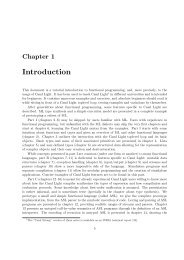
Chapter 1 : This chapter describes how to install version 2.04 of the <strong>Objective</strong> <strong>Caml</strong><br />
<strong>language</strong> on the most current systems (Windows, Unix and MacOS).<br />
Part I: Core of the <strong>language</strong> <strong>The</strong> first part is a complete presentation of the basic<br />
elements of the <strong>Objective</strong> <strong>Caml</strong> <strong>language</strong>. Chapter 2 is a dive into the functional<br />
core of the <strong>language</strong>. Chapter 3 is a continuation of the previous one and<br />
describes the imperative part of the <strong>language</strong>. Chapter 4 compares the “pure”<br />
functional and imperative styles, then presents their joint use. Chapter 5 presents<br />
the graphics library. Chapter 6 exhibits three applications: management of a<br />
simple database, a mini-Basic interpreter and a well-known single-player game,<br />
minesweeper.<br />
Part II: Development tools <strong>The</strong> second part of the book describes the various tools<br />
for application development. Chapter 7 compares the various compilation modes,<br />
which are the interactive toplevel and command-line bytecode and native code<br />
compilers. Chapter 8 presents the principal libraries provided with the <strong>language</strong><br />
distribution. Chapter 9 explains garbage collection mechanisms and details the<br />
one used by <strong>Objective</strong> <strong>Caml</strong>. Chapter 10 explains the use of tools for debugging<br />
and profiling programs. Chapter 11 addresses lexical and syntactic tools.<br />
Chapter 12 shows how to interface <strong>Objective</strong> <strong>Caml</strong> programs with C. Chapter<br />
13 constructs a library and an application. This library offers tools for the construction<br />
of GUIs. <strong>The</strong> application is a search for least-cost paths within a graph,<br />
whose GUI uses the preceding library.<br />
Part III: Organization of applications <strong>The</strong> third part describes the two ways of<br />
organizing a program: with modules, and with objects. Chapter 14 is a presentation<br />
of simple and parameterized <strong>language</strong> modules. Chapter 15 introduces <strong>Objective</strong><br />
<strong>Caml</strong> object-oriented extension. Chapter 16 compares these two types of<br />
organization and indicates the usefulness of mixing them to increase the extensibility<br />
of programs. Chapter 17 describes two substantial applications: two-player<br />
games which put to work several parameterized modules used for two different<br />
games, and a simulation of a robot world demonstrating interobject communication.<br />
Part IV: Concurrence and distribution <strong>The</strong> fourth part introduces concurrent<br />
and distributed programs while detailing communication between processes, lightweight<br />
or not, and on the Internet. Chapter 18 demonstrates the direct link between<br />
the <strong>language</strong> and the system libraries, in particular the notions of process and
xxvi Introduction<br />
communication. Chapter 19 leads to the lack of determinism of concurrent programming<br />
while presenting <strong>Objective</strong> <strong>Caml</strong>’s threads. Chapter 20 discusses interprocess<br />
communication via sockets in the distributed memory model. Chapter<br />
21 presents first of all a toolbox for client-server applications. It is subsequently<br />
used to extend the robots of the previous part to the client-server model. Finally,<br />
we adapt some of the programs already encountered in the form of an HTTP<br />
server.<br />
Chapter 22 This last chapter takes stock of application development in <strong>Objective</strong><br />
<strong>Caml</strong> and presents the best-known applications of the ML <strong>language</strong> family.<br />
Appendices <strong>The</strong> first appendix explains the notion of cyclic types used in the typing<br />
of objects. <strong>The</strong> second appendix describes the <strong>language</strong> changes present in<br />
the new version 3.00. <strong>The</strong>se have been integrated in all following versions of<br />
<strong>Objective</strong> <strong>Caml</strong> (3.xx).<br />
Each chapter consists of a general presentation of the subject being introduced, a<br />
chapter outline, the various sections thereof, statements of exercises to carry out, a<br />
summary, and a final section entitled “To learn more” which indicates bibliographic<br />
references for the subject which has been introduced.
1<br />
How to obtain<br />
<strong>Objective</strong> <strong>Caml</strong><br />
<strong>The</strong> various programs used in this work are “free” software 1 . <strong>The</strong>y can be found either<br />
on the CD-ROM accompanying this work, or by downloading them from the Internet.<br />
This is the case for <strong>Objective</strong> <strong>Caml</strong>, developed at <strong>Inria</strong>.<br />
Description of the CD-ROM<br />
<strong>The</strong> CD-ROM is provided as a hierarchy of files. At the root can be found the file<br />
index.html which presents the CD-ROM, as well as the five subdirectories below:<br />
• book: root of the HTML version of the book along with the solutions to the<br />
exercises;<br />
• apps: applications described in the book;<br />
• exercises: independent solutions to the proposed exercises;<br />
• distrib: set of distributions provided by <strong>Inria</strong>, as described in the next section;<br />
• tools: set of tools for development in <strong>Objective</strong> <strong>Caml</strong>;<br />
• docs: online documentation of the distribution and the tools.<br />
To read the CD-ROM, start by opening the file index.html in the root using your<br />
browser of choice. To access directly the hypertext version of the book, open the file<br />
book/index.html. This file hierarchy, updated in accordance with readers’ remarks,<br />
can be found posted on the editor’s site:<br />
Link: http://www.oreilly.fr<br />
1. “Free software” is not to be confused with “freeware”. “Freeware” is software which costs nothing,<br />
whereas “free software” is software whose source is also freely available. In the present case, all the<br />
programs used cost nothing and their source is available.
2 Chapter 1 : How to obtain <strong>Objective</strong> <strong>Caml</strong><br />
Downloading<br />
<strong>Objective</strong> <strong>Caml</strong> can be downloaded via web browser at the following address:<br />
Link: http://caml.inria.fr/ocaml/distrib.html<br />
<strong>The</strong>re one can find binary distributions for Linux (Intel and PPC), for Windows (NT,<br />
95, 98) and for MacOS (7, 8), as well as documentation, in English, in different formats<br />
(PDF, PostScript and HTML). <strong>The</strong> source code for the three systems is available<br />
for download as well. Once the desired distribution is copied to one’s machine, it’s time<br />
to install it. This procedure varies according to the operating system used.<br />
Installation<br />
Installing <strong>Objective</strong> <strong>Caml</strong> requires about 10MB of free space on one’s hard disk drive.<br />
<strong>The</strong> software can easily be uninstalled without corrupting the system.<br />
Installation under Windows<br />
<strong>The</strong> file containing the binary distribution is called: ocaml-2.04-win.zip, indicating<br />
the version number (here 2.04) and the operating system.<br />
Warning<br />
<strong>Objective</strong> <strong>Caml</strong> only works under recent versions of<br />
Windows : Windows 95, 98 and NT. Don’t try to install<br />
it under Windows 3.x or OS2/Warp.<br />
1. <strong>The</strong> file is in compressed (.zip) format; the first thing to do is decompress it.<br />
Use your favorite decompression software for this. You obtain in this way a file<br />
hierarchy whose root is named ocaml. You can place this directory at any location<br />
on your hard disk. It is denoted by in what follows.<br />
2. This directory includes:<br />
• two subdirectories: bin for binaries and lib for libraries;<br />
• two “text” files: License.txt and Changes.txt containing the license to<br />
use the software and the changes relative to previous versions;<br />
• an application: O<strong>Caml</strong>Win corresponding to the main application;<br />
• a configuration file: Ocamlwin.ini which will need to be modified (see the<br />
following point);<br />
• two files of version notes: the first, Readme.gen, for this version and the<br />
second, Readme.win, for the version under Windows.<br />
3. If you have chosen a directory other than c:\ocaml as the root of your file<br />
hierarchy, then it is necessary to indicate this in the configuration file. Edit it<br />
with Wordpad and change the line defining CmdLine which is of the form:<br />
CmdLine=ocamlrun c:\ocaml\bin\ocaml.exe -I c:\ocaml\lib<br />
to
Installation 3<br />
CmdLine=ocamlrun \bin\ocaml.exe -I \lib<br />
You have to replace the names of the search paths for binaries and libraries with<br />
the name of the <strong>Objective</strong> <strong>Caml</strong> root directory. If we have chosen C:\Lang\ocaml<br />
as the root directory (), the modification becomes:<br />
CmdLine=ocamlrun C:\Lang\ocaml\bin\ocaml.exe -I C:\Lang\ocaml\lib<br />
4. Copy the file O<strong>Caml</strong>Win.ini to the main system directory, that is, C:\windows<br />
or C:\win95 or C:\winnt according to the installation of your system.<br />
Now it’s time to test the O<strong>Caml</strong>Win application by double-clicking on it. You’ll get the<br />
window in figure 1.1.<br />
Figure 1.1: <strong>Objective</strong> <strong>Caml</strong> window under Windows.<br />
<strong>The</strong> configuration of command-line executables, launched from a DOS window, is done<br />
by modifying the PATH variable and the <strong>Objective</strong> <strong>Caml</strong> library search path variable<br />
(CAMLLIB), as follows:<br />
PATH=%PATH%;\bin<br />
set CAMLLIB=\lib<br />
where is replaced by the path where <strong>Objective</strong> <strong>Caml</strong> is installed.
4 Chapter 1 : How to obtain <strong>Objective</strong> <strong>Caml</strong><br />
<strong>The</strong>se two commands can be included in the autoexec.bat file which every good DOS<br />
has. To test the command-line executables, type the command ocaml in a DOS window.<br />
This executes the file:<br />
/bin/ocaml.exe<br />
corresponding to the <strong>Objective</strong> <strong>Caml</strong>. text mode toplevel. To exit from this command,<br />
type #quit;;.<br />
To install <strong>Objective</strong> <strong>Caml</strong> from source under Windows is not so easy, because it requires<br />
the use of commercial software, in particular the Microsoft C compiler. Refer to the<br />
file Readme.win of the binary distribution to get the details.<br />
Installation under Linux<br />
<strong>The</strong> Linux installation also has an easy-to-install binary distribution in the form of an<br />
rpm. package. Installation from source is described in section 1. <strong>The</strong> file to download<br />
is: ocaml-2.04-2.i386.rpm which will be used as follows with root privileges:<br />
rpm -i ocaml-2.04-2.i386.rpm<br />
which installs the executables in the /usr/bin directory and the libraries in the<br />
/usr/lib/ocaml directory.<br />
To test the installation, type: ocamlc -v which prints the version of <strong>Objective</strong> <strong>Caml</strong><br />
installed on the machine.<br />
ocamlc -v<br />
<strong>The</strong> <strong>Objective</strong> <strong>Caml</strong> compiler, version 2.04<br />
Standard library directory: /usr/lib/ocaml<br />
You can also execute the command ocaml which prints the header of the interactive<br />
toplevel.<br />
#<br />
<strong>Objective</strong> <strong>Caml</strong> version 2.04<br />
<strong>The</strong> # character is the prompt in the interactive toplevel. This interactive toplevel can<br />
be exited by the #quit;; directive, or by typing CTRL-D. <strong>The</strong> two semi-colons indicate<br />
the end of an <strong>Objective</strong> <strong>Caml</strong> phrase.<br />
Installation under MacOS<br />
<strong>The</strong> MacOS distribution is also in the form of a self-extracting binary. <strong>The</strong> file to<br />
download is: ocaml-2.04-mac.sea.bin which is compressed. Use your favorite software
Testing the installation 5<br />
to decompress it. <strong>The</strong>n all you have to do to install it is launch the self-extracting<br />
archive and follow the instructions printed in the dialog box to choose the location<br />
of the distribution. For the MacOS X server distribution, follow the installation from<br />
source under Unix.<br />
Installation from source under Unix<br />
<strong>Objective</strong> <strong>Caml</strong> can be installed on systems in the Unix family from the source distribution.<br />
Indeed it will be necessary to compile the <strong>Objective</strong> <strong>Caml</strong> system. To do<br />
this, one must either have a C compiler on one’s Unix, machine, which is generally<br />
the case, or download one such as gcc which works on most Unix. systems. <strong>The</strong> <strong>Objective</strong><br />
<strong>Caml</strong> distribution file containing the source is: ocaml-2.04.tar.gz. <strong>The</strong> file<br />
INSTALL describes, in a very clear way, the various stages of configuring, making, and<br />
then installing the binaries.<br />
Installation of the HTML documentation<br />
<strong>Objective</strong> <strong>Caml</strong>’s English documentation is present also in the form of a hierarchy of<br />
HTML files which can be found in the docs directory of the CD-ROM.<br />
This documentation is a reference manual. It is not easy reading for the beginner.<br />
Nevertheless it is quite useful as a description of the <strong>language</strong>, its tools, and its libraries.<br />
It will soon become indispensable for anyone who hopes to write a program of more<br />
than ten lines.<br />
Testing the installation<br />
Once installation of the <strong>Objective</strong> <strong>Caml</strong> development environment is done, it is necessary<br />
to test it, mainly to verify the search paths for executables and libraries. <strong>The</strong><br />
simplest way is to launch the interactive toplevel of the system and write the first little<br />
program that follows:<br />
String.concat "/" ["a"; "path"; "here"] ;;<br />
This expression concatenates several character strings, inserting the “/” character between<br />
each word. <strong>The</strong> notation String.concat indicates use of the function concat<br />
from the String. If the library search path is not correct, the system will print an error.<br />
It will be noted that the system indicates that the computation returns a character<br />
string and prints the result.<br />
<strong>The</strong> documentation of this function String.concat can be found in the online reference<br />
manual by following the links “<strong>The</strong> standard library” then “Module String: string<br />
operations”.<br />
To exit the interactive toplevel, the user must type the directive “#quit ;;”.
6 Chapter 1 : How to obtain <strong>Objective</strong> <strong>Caml</strong>
Part I<br />
Language Core<br />
7
<strong>The</strong> first part of this book is a complete introduction to the core of the <strong>Objective</strong><br />
<strong>Caml</strong> <strong>language</strong>, in particular the expression evaluation mechanism, static typing and<br />
the data memory model.<br />
An expression is the description of a computation. Evaluation of an expression returns<br />
a value at the end of the computation. <strong>The</strong> execution of an <strong>Objective</strong> <strong>Caml</strong> program<br />
corresponds to the computation of an expression. Functions, program execution control<br />
structures, even conditions or loops, are themselves also expressions.<br />
Static typing guarantees that the computation of an expression cannot cause a run-time<br />
type error. In fact, application of a function to some arguments (or actual parameters)<br />
isn’t accepted unless they all have types compatible with the formal parameters indicated<br />
in the definition of the function. Furthermore, the <strong>Objective</strong> <strong>Caml</strong> <strong>language</strong> has<br />
type infererence: the compiler automatically determines the most general type of an<br />
expression.<br />
Finally a minimal knowledge of the representation of data is indispensable to the<br />
programmer in order to master the effects of physical modifications to the data.<br />
Outline<br />
Chapter 2 contains a complete presentation of the purely functional part of the <strong>language</strong><br />
and the constraints due to static typing. <strong>The</strong> notion of expression evaluation is<br />
illustrated there at length. <strong>The</strong> following control structures are detailed: conditional,<br />
function application and pattern matching. <strong>The</strong> differences between the type and the<br />
domain of a function are discussed in order to introduce the exception mechanism. This<br />
feature of the <strong>language</strong> goes beyond the functional context and allows management of<br />
computational breakdowns.<br />
Chapter 3 exhibits the imperative style. <strong>The</strong> constructions there are closer to classic<br />
<strong>language</strong>s. Associative control structures such as sequence and iteration are presented<br />
there, as well as mutable data structures. <strong>The</strong> interaction between physical modifications<br />
and sharing of data is then detailed. Type inference is described there in the<br />
context of these new constructions.<br />
Chapter 4 compares the two preceding styles and especially presents different mixed<br />
styles. This mixture supports in particular the construction of lazy data structures,<br />
including mutable ones.<br />
Chapter 5 demonstrates the use of the Graphics library included in the <strong>language</strong><br />
distribution. <strong>The</strong> basic notions of graphics programming are exhibited there and immediately<br />
put into practice. <strong>The</strong>re’s even something about GUI construction thanks<br />
to the minimal event control provided by this library.<br />
<strong>The</strong>se first four chapters are illustrated by a complete example, the implementation<br />
of a calculator, which evolves from chapter to chapter.<br />
Chapter 6 presents three complete applications: a little database, a mini-BASIC interpreter<br />
and the game Minesweeper. <strong>The</strong> first two examples are constructed mainly in a<br />
functional style, while the third is done in an imperative style.<br />
9
10<br />
<strong>The</strong> rudiments of syntax<br />
Before beginning we indicate the first elements of the syntax of the <strong>language</strong>. A program<br />
is a sequence of phrases in the <strong>language</strong>. A phrase is a complete, directly executable<br />
syntactic element (an expression, a declaration). A phrase is terminated with a double<br />
semi-colon (; ;). <strong>The</strong>re are three different types of declarations which are each marked<br />
with a different keyword:<br />
value declaration : let<br />
exception declaration : exception<br />
type declaration : type<br />
All the examples given in this part are to be input into the interactive toplevel of the<br />
<strong>language</strong>.<br />
Here’s a first (little) <strong>Objective</strong> <strong>Caml</strong> program, to be entered into the toplevel, whose<br />
prompt is the pound character (#), in which a function fact computing the factorial<br />
of a natural number, and its application to a natural number 8, are defined.<br />
# let rec fact n = if n < 2 then 1 else n * fact(n-1) ; ;<br />
val fact : int -> int = <br />
# fact 8 ; ;<br />
- : int = 40320<br />
This program consists of two phrases. <strong>The</strong> first is the declaration of a function value<br />
and the second is an expression. One sees that the toplevel prints out three pieces<br />
of information which are: the name being declared, or a dash (-) in the case of an<br />
expression; the inferred type; and the return value. In the case of a function value, the<br />
system prints .<br />
<strong>The</strong> following example demonstrates the manipulation of functions as values in the<br />
<strong>language</strong>. <strong>The</strong>re we first of all define the function succ which calculates the successor<br />
of an integer, then the function compose which composes two functions. <strong>The</strong> latter will<br />
be applied to fact and succ.<br />
# let succ x = x+1 ; ;<br />
val succ : int -> int = <br />
# let compose f g x = f(g x) ; ;<br />
val compose : (’a -> ’b) -> (’c -> ’a) -> ’c -> ’b = <br />
# compose fact succ 8 ; ;<br />
- : int = 362880<br />
This last call carries out the computation fact(succ 8) and returns the expected<br />
result. Let us note that the functions fact and succ are passed as parameters to<br />
compose in the same way as the natural number 8.
2<br />
Functional<br />
programming<br />
<strong>The</strong> first functional <strong>language</strong>, Lisp, appeared at the end of the 1950’s. That is, at<br />
the same time as Fortran, the first representative of the imperative <strong>language</strong>s. <strong>The</strong>se<br />
two <strong>language</strong>s still exist, although both have evolved greatly. <strong>The</strong>y are used widely for<br />
numerical programming (in the case of Fortran) and symbolic applications in the case of<br />
Lisp. Interest in functional programming arises from the great ease of writing programs<br />
and specifying the values which they manipulate. A program is a function applied to its<br />
arguments. It computes a result which is returned (when the computation terminates)<br />
as the output of the program. In this way it becomes easy to combine programs: the<br />
output of one program becomes an input argument to another, in the sense of function<br />
composition.<br />
Functional programming is based on a simple computation model with three constructions:<br />
variables, function definitions, and applications of a function to an argument.<br />
This model is called the λ-calculus and it was introduced by Alonzo Church in 1932,<br />
thus before the first computer. It was created to offer a general theoretical model of<br />
the notion of computability. In the λ-calculus, all functions are values which can be<br />
manipulated. <strong>The</strong>y can be used as arguments to other functions, or returned as the<br />
result of a call to another function. <strong>The</strong> theory of λ-calculus asserts that everything<br />
which is computable (i.e., programmable) can be written in this formalism. Its syntax<br />
is too limited to make its use as a programming <strong>language</strong> practical, so primitive values<br />
(such as integers or character strings), operations on these primitive values, control<br />
structures, and declarations which allow the naming of values or functions and, in<br />
particular, recursive functions, have all been added to the λ-calculus to make it more<br />
palatable.<br />
<strong>The</strong>re are several classifications of functional <strong>language</strong>s. For our part, we will distinguish<br />
them according to two characteristics which seem to us most salient:<br />
• Without side effects (pure) or with side effects (impure): a pure functional <strong>language</strong><br />
is a <strong>language</strong> in which there is no change of state. <strong>The</strong>re everything is<br />
simply a computation and the way it is carried out is unimportant. Impure func-
12 Chapter 2 : Functional programming<br />
tional <strong>language</strong>s, such as Lisp or ML, integrate imperative traits such as change<br />
of state. <strong>The</strong>y permit the writing of algorithms in a style closer to <strong>language</strong>s like<br />
Fortran, where the order of evaluation of expressions is significant.<br />
• Dynamically typed or statically typed: typing permits verification of whether<br />
an argument passed to a function is indeed of the type of the function’s formal<br />
parameter. This verification can be made during program execution. In that case<br />
this verification is called dynamic typing. If type errors occur the program will<br />
halt in a consistent state. This is the case in the <strong>language</strong> Lisp. This verification<br />
can also be done before program execution, that is, at compilation time. This a<br />
priori verification is called static typing. Having been carried out once and for all,<br />
it won’t slow down program execution. This is the case in the ML <strong>language</strong> and<br />
its dialects such as <strong>Objective</strong> <strong>Caml</strong>. Only correctly typed programs, i.e., those<br />
accepted by the type verifier, will be able to be compiled and then executed.<br />
Chapter outline<br />
This chapter presents the basic elements of the functional part of the <strong>Objective</strong> <strong>Caml</strong><br />
<strong>language</strong>, namely its syntactic elements, its <strong>language</strong> of types and its exception mechanism.<br />
This will lead us to the development of a first example of a complete program.<br />
<strong>The</strong> first section describes the core of the <strong>language</strong>, beginning with primitive values<br />
and the functions which manipulate them. We then go on to structured values and to<br />
function values. <strong>The</strong> basic control structures are introduced as well as local and global<br />
value declarations. <strong>The</strong> second section deals with type definitions for the construction<br />
of structured values and with pattern matching to access these structures. <strong>The</strong> third<br />
section compares the inferred type of functions and their domain of definition, which<br />
leads us to introduce the exception mechanism. <strong>The</strong> fourth section illustrates all these<br />
notions put together, by describing a simple application: a desktop calculator.<br />
Functional core of <strong>Objective</strong> <strong>Caml</strong><br />
Like all functional <strong>language</strong>s, <strong>Objective</strong> <strong>Caml</strong> is an expression oriented <strong>language</strong>, where<br />
programming consists mainly of creating functions and applying them. <strong>The</strong> result of<br />
the evaluation of one of these expressions is a value in the <strong>language</strong> and the execution<br />
of a program is the evaluation of all the expressions which comprise it.<br />
Primitive values, functions, and types<br />
Integers and floating-point numbers, characters, character strings, and booleans are<br />
predefined in <strong>Objective</strong> <strong>Caml</strong>.
Functional core of <strong>Objective</strong> <strong>Caml</strong> 13<br />
Numbers<br />
<strong>The</strong>re are two kinds of numbers: integers 1 of type int and floating-point numbers of<br />
type float. <strong>Objective</strong> <strong>Caml</strong> follows the IEEE 754 standard 2 for representing doubleprecision<br />
floating-point numbers. <strong>The</strong> operations on integers and floating-point numbers<br />
are described in figure 2.1. Let us note that when the result of an integer operation<br />
is outside the interval on which values of type int are defined, this does not produce<br />
an error, but the result is an integer within the system’s interval of integers. In other<br />
words, all integer operations are operations modulo the boundaries of the interval.<br />
integer numbers floating-point numbers<br />
+ addition<br />
- subtraction and unary negation<br />
* multiplication<br />
/ integer division<br />
mod remainder of integer division<br />
# 1 ; ;<br />
- : int = 1<br />
# 1 + 2 ; ;<br />
- : int = 3<br />
# 9 / 2 ; ;<br />
- : int = 4<br />
# 11 mod 3 ; ;<br />
- : int = 2<br />
(* limits of the representation *)<br />
(* of integers *)<br />
# 2147483650 ; ;<br />
- : int = 2<br />
Figure 2.1: Operations on numbers.<br />
+. addition<br />
-. subtraction and unary negation<br />
*. multiplication<br />
/. division<br />
** exponentiation<br />
# 2.0 ; ;<br />
- : float = 2<br />
# 1.1 +. 2.2 ; ;<br />
- : float = 3.3<br />
# 9.1 /. 2.2 ; ;<br />
- : float = 4.13636363636<br />
# 1. /. 0. ; ;<br />
- : float = inf<br />
(* limits of the representation *)<br />
(* of floating-point numbers *)<br />
# 222222222222.11111 ; ;<br />
- : float = 222222222222<br />
Differences between integers and floating-point numbers Values having different<br />
types such as float and int can never be compared directly. But there are<br />
functions for conversion (float of int and int of float) between one and the other.<br />
# 2 = 2.0 ; ;<br />
Characters 5-8:<br />
This expression has type float but is here used with type int<br />
# 3.0 = float of int 3 ; ;<br />
1. In the interval [−2 30 , 2 30 − 1] on 32-bit machines and in the interval [−2 62 , 2 62 − 1] on 64-bit<br />
machines<br />
2. <strong>The</strong> floating point number m × 10 n is represented with a 53-bit mantissa m and an exponent n in<br />
the interval [−1022, 1023].
14 Chapter 2 : Functional programming<br />
- : bool = true<br />
In the same way, operations on floating-point numbers are distinct from those on<br />
integers.<br />
# 3 + 2 ; ;<br />
- : int = 5<br />
# 3.0 +. 2.0 ; ;<br />
- : float = 5<br />
# 3.0 + 2.0 ; ;<br />
Characters 0-3:<br />
This expression has type float but is here used with type int<br />
# sin 3.14159 ; ;<br />
- : float = 2.65358979335e-06<br />
An ill-defined computation, such as a division by zero, will raise an exception (see page<br />
54) which interrupts the computation. Floating-point numbers have a representation<br />
for infinite values (printed as Inf) and ill-defined computations (printed as NaN 3 ). <strong>The</strong><br />
main functions on floating-point numbers are described in figure 2.2.<br />
3. Not a Number<br />
functions on floats trigonometric functions<br />
ceil<br />
floor<br />
sqrt square root<br />
exp exponential<br />
log natural log<br />
log10 log base 10<br />
# ceil 3.4 ; ;<br />
- : float = 4<br />
# floor 3.4 ; ;<br />
- : float = 3<br />
# ceil (-.3.4) ; ;<br />
- : float = -3<br />
# floor (-.3.4) ; ;<br />
- : float = -4<br />
cos cosine<br />
sin sine<br />
tan tangent<br />
acos arccosine<br />
asin arcsine<br />
atan arctangent<br />
Figure 2.2: Functions on floats.<br />
# sin 1.57078 ; ;<br />
- : float = 0.999999999867<br />
# sin (asin 0.707) ; ;<br />
- : float = 0.707<br />
# acos 0.0 ; ;<br />
- : float = 1.57079632679<br />
# asin 3.14 ; ;<br />
- : float = nan
Functional core of <strong>Objective</strong> <strong>Caml</strong> 15<br />
Characters and Strings<br />
Characters, type char, correspond to integers between 0 and 255 inclusive, following<br />
the ASCII encoding for the first 128. <strong>The</strong> functions char of int and int of char<br />
support conversion between integers and characters. Character strings, type string,<br />
are sequences of characters of definite length (less than 2 24 − 6). <strong>The</strong> concatenation<br />
operator is ^ . <strong>The</strong> functions int of string, string of int, string of float and<br />
float of string carry out the various conversions between numbers and character<br />
strings.<br />
# ’B’ ; ;<br />
- : char = ’B’<br />
# int of char ’B’ ; ;<br />
- : int = 66<br />
# "is a string" ; ;<br />
- : string = "is a string"<br />
# (string of int 1987) ^ " is the year <strong>Caml</strong> was created" ; ;<br />
- : string = "1987 is the year <strong>Caml</strong> was created"<br />
Even if a string contains the characters of a number, it won’t be possible to use it in<br />
operations on numbers without carrying out an explicit conversion.<br />
# "1999" + 1 ; ;<br />
Characters 1-7:<br />
This expression has type string but is here used with type int<br />
# (int of string "1999") + 1 ; ;<br />
- : int = 2000<br />
Numerous functions on character strings are gathered in the String module (see page<br />
217).<br />
Booleans<br />
Booleans, of type bool, belong to a set consisting of two values: true and false. <strong>The</strong><br />
primitive operators are described in figure 2.3. For historical reasons, the “and” and<br />
“or” operators each have two forms.<br />
# true ; ;<br />
- : bool = true<br />
# not true ; ;<br />
- : bool = false<br />
not negation<br />
&& sequential and<br />
|| sequential or<br />
& synonym for &&<br />
or synonym for ||<br />
Figure 2.3: Operators on booleans.
16 Chapter 2 : Functional programming<br />
# true && false ; ;<br />
- : bool = false<br />
<strong>The</strong> operators && and ||, or their synonyms, evaluate their left argument and then,<br />
depending on its value, evaluate their right argument. <strong>The</strong>y can be rewritten in the<br />
form of conditional constructs (see page 18).<br />
= structural equality<br />
== physical equality<br />
negation of =<br />
!= negation of ==<br />
< less than<br />
> greater than<br />
= greater than or equal to<br />
Figure 2.4: Equality and comparison operators.<br />
<strong>The</strong> equality and comparison operators are described in figure 2.4. <strong>The</strong>y are polymorphic,<br />
i.e., they can be used to compare two integers as well as two character strings.<br />
<strong>The</strong> only constraint is that their two operands must be of the same type (see page 28).<br />
# 1
Functional core of <strong>Objective</strong> <strong>Caml</strong> 17<br />
Cartesian product, tuple<br />
Values of possibly different types can be gathered in pairs or more generally in tuples.<br />
<strong>The</strong> values making up a tuple are separated by commas. <strong>The</strong> type constructor * indicates<br />
a tuple. <strong>The</strong> type int * string is the type of pairs whose first element is an<br />
integer (of type int) and whose second is a character string (of type string).<br />
# ( 12 , "October" ) ; ;<br />
- : int * string = 12, "October"<br />
When there is no ambiguity, it can be written more simply:<br />
# 12 , "October" ; ;<br />
- : int * string = 12, "October"<br />
<strong>The</strong> functions fst and snd allow access to the first and second elements of a pair.<br />
# fst ( 12 , "October" ) ; ;<br />
- : int = 12<br />
# snd ( 12 , "October" ) ; ;<br />
- : string = "October"<br />
<strong>The</strong>se two functions accept pairs whose components are of any type whatsoever. <strong>The</strong>y<br />
are polymorphic, in the same way as equality.<br />
# fst; ;<br />
- : ’a * ’b -> ’a = <br />
# fst ( "October", 12 ) ; ;<br />
- : string = "October"<br />
<strong>The</strong> type int * char * string is that of triplets whose first element is of type int,<br />
whose second is of type char, and whose third is of type string. Its values are written<br />
# ( 65 , ’B’ , "ascii" ) ; ;<br />
- : int * char * string = 65, ’B’, "ascii"<br />
Warning<br />
<strong>The</strong> functions fst and snd applied to a tuple, other<br />
than a pair, result in a type error.<br />
# snd ( 65 , ’B’ , "ascii" ) ; ;<br />
Characters 7-25:<br />
This expression has type int * char * string but is here used with type<br />
’a * ’b<br />
<strong>The</strong>re is indeed a difference between the type of a pair and that of a triplet. <strong>The</strong> type<br />
int * int * int is different from the types (int * int) * int and int * (int *<br />
int). Functions to access a triplet (and other tuples) are not defined by the core library.<br />
One can use pattern matching to define them if need be (see page 34).<br />
Lists<br />
Values of the same type can be gathered into a list. A list can either be empty or<br />
consist of elements of the same type.<br />
# [] ; ;<br />
- : ’a list = []
18 Chapter 2 : Functional programming<br />
# [ 1 ; 2 ; 3 ] ; ;<br />
- : int list = [1; 2; 3]<br />
# [ 1 ; "two" ; 3 ] ; ;<br />
Characters 14-17:<br />
This expression has type int list but is here used with type string list<br />
<strong>The</strong> function which adds an element at the head of a list is the infix operator :: . It is<br />
the analogue of Lisp’s cons.<br />
# 1 :: 2 :: 3 :: [] ; ;<br />
- : int list = [1; 2; 3]<br />
Concatenation of two lists is also an infix operator @.<br />
# [ 1 ] @ [ 2 ; 3 ] ; ;<br />
- : int list = [1; 2; 3]<br />
# [ 1 ; 2 ] @ [ 3 ] ; ;<br />
- : int list = [1; 2; 3]<br />
<strong>The</strong> other list manipulation functions are defined in the List library. <strong>The</strong> functions<br />
hd and tl from this library give respectively the head and the tail of a list when these<br />
values exist. <strong>The</strong>se functions are denoted by List.hd and List.tl to indicate to the<br />
system that they can be found in the module List 4 .<br />
# List.hd [ 1 ; 2 ; 3 ] ; ;<br />
- : int = 1<br />
# List.hd [] ; ;<br />
Uncaught exception: Failure("hd")<br />
In this last example, it is indeed problematic to request retrieval of the first element<br />
of an empty list. It is for this reason that the system raises an exception (see page 54).<br />
Conditional control structure<br />
One of the indispensable control structures in any programming <strong>language</strong> is the structure<br />
called conditional (or branch) which guides the computation as a function of a<br />
condition.<br />
Syntax : if expr1 then expr2 else expr3<br />
<strong>The</strong> expression expr1 is of type bool. <strong>The</strong> expressions expr2 and expr3 must be of the<br />
same type, whatever it may be.<br />
# if 3=4 then 0 else 4 ; ;<br />
- : int = 4<br />
# if 3=4 then "0" else "4" ; ;<br />
4. <strong>The</strong> List module is presented on page 217.
Functional core of <strong>Objective</strong> <strong>Caml</strong> 19<br />
- : string = "4"<br />
# if 3=4 then 0 else "4"; ;<br />
Characters 20-23:<br />
This expression has type string but is here used with type int<br />
A conditional construct is itself an expression and its evaluation returns a value.<br />
# (if 3=5 then 8 else 10) + 5 ; ;<br />
- : int = 15<br />
Note<br />
<strong>The</strong> else branch can be omitted, but in this case it is implicitly replaced<br />
by else (). Consequently, the type of the expression expr2 must be unit<br />
(see page 79).<br />
Value declarations<br />
A declaration binds a name to a value. <strong>The</strong>re are two types: global declarations and<br />
local declarations. In the first case, the declared names are known to all the expressions<br />
following the declaration; in the second, the declared names are only known to one<br />
expression. It is equally possible to simultaneously declare several name-value bindings.<br />
Global declarations<br />
Syntax : let name = expr ;;<br />
A global declaration defines the binding between the name name and the value of the<br />
expression expr which will be known to all subsequent expressions.<br />
# let yr = "1999" ; ;<br />
val yr : string = "1999"<br />
# let x = int of string(yr) ; ;<br />
val x : int = 1999<br />
# x ; ;<br />
- : int = 1999<br />
# x + 1 ; ;<br />
- : int = 2000<br />
# let new yr = string of int (x + 1) ; ;<br />
val new_yr : string = "2000"
20 Chapter 2 : Functional programming<br />
Simultaneous global declarations<br />
Syntax :<br />
let name1 = expr1<br />
and name2 = expr2<br />
.<br />
and namen = exprn ;;<br />
A simultaneous declaration declares different symbols at the same level. <strong>The</strong>y won’t<br />
be known until the end of all the declarations.<br />
# let x = 1 and y = 2 ; ;<br />
val x : int = 1<br />
val y : int = 2<br />
# x + y ; ;<br />
- : int = 3<br />
# let z = 3 and t = z + 2 ; ;<br />
Characters 18-19:<br />
Unbound value z<br />
It is possible to gather several global declarations in the same phrase; then printing of<br />
their types and their values does not take place until the end of the phrase, marked by<br />
double “;;”. <strong>The</strong>se declarations are evaluated sequentially, in contrast with a simultaneous<br />
declaration.<br />
# let x = 2<br />
let y = x + 3 ; ;<br />
val x : int = 2<br />
val y : int = 5<br />
A global declaration can be masked by a new declaration of the same name (see page<br />
26).<br />
Local declarations<br />
Syntax : let name = expr1 in expr2;;<br />
<strong>The</strong> name name is only known during the evaluation of expr2. <strong>The</strong> local declaration<br />
binds it to the value of expr1.<br />
# let xl = 3 in xl * xl ; ;<br />
- : int = 9<br />
<strong>The</strong> local declaration binding xl to the value 3 is only in effect during the evaluation<br />
of xl * xl.<br />
# xl ; ;<br />
Characters 1-3:<br />
Unbound value xl<br />
A local declaration masks all previous declarations of the same name, but the previous<br />
value is reinstated upon leaving the scope of the local declaration:<br />
# let x = 2 ; ;
Functional core of <strong>Objective</strong> <strong>Caml</strong> 21<br />
val x : int = 2<br />
# let x = 3 in x * x ; ;<br />
- : int = 9<br />
# x * x ; ;<br />
- : int = 4<br />
A local declaration is an expression and can thus be used to construct other expressions:<br />
# (let x = 3 in x * x) + 1 ; ;<br />
- : int = 10<br />
Local declarations can also be simultaneous.<br />
Syntax :<br />
let name1 = expr1<br />
and name2 = expr2<br />
.<br />
.<br />
and namen = exprn<br />
in expr ;;<br />
# let a = 3.0 and b = 4.0 in sqrt (a*.a +. b*.b) ; ;<br />
- : float = 5<br />
# b ; ;<br />
Characters 0-1:<br />
Unbound value b<br />
Function expressions, functions<br />
A function expression consists of a parameter and a body. <strong>The</strong> formal parameter is a<br />
variable name and the body an expression. <strong>The</strong> parameter is said to be abstract. For<br />
this reason, a function expression is also called an abstraction.<br />
Syntax : function p –> expr<br />
Thus the function which squares its argument is written:<br />
# function x → x*x ; ;<br />
- : int -> int = <br />
<strong>The</strong> <strong>Objective</strong> <strong>Caml</strong> system deduces its type. <strong>The</strong> function type int -> int indicates<br />
a function expecting a parameter of type int and returning a value of type int.<br />
Application of a function to an argument is written as the function followed by the<br />
argument.<br />
# (function x → x * x) 5 ; ;<br />
- : int = 25<br />
<strong>The</strong> evaluation of an application amounts to evaluating the body of the function, here
22 Chapter 2 : Functional programming<br />
x * x, where the formal parameter, x, is replaced by the value of the argument (or the<br />
actual parameter), here 5.<br />
In the construction of a function expression, expr is any expression whatsoever. In<br />
particular, expr may itself be a function expression.<br />
# function x → (function y → 3*x + y) ; ;<br />
- : int -> int -> int = <br />
<strong>The</strong> parentheses are not required. One can write more simply:<br />
# function x → function y → 3*x + y ; ;<br />
- : int -> int -> int = <br />
<strong>The</strong> type of this expression can be read in the usual way as the type of a function which<br />
expects two integers and returns an integer value. But in the context of a functional<br />
<strong>language</strong> such as <strong>Objective</strong> <strong>Caml</strong> we are dealing more precisely with the type of a<br />
function which expects an integer and returns a function value of type int -> int:<br />
# (function x → function y → 3*x + y) 5 ; ;<br />
- : int -> int = <br />
One can, of course, use the function expression in the usual way by applying it to two<br />
arguments. One writes:<br />
# (function x → function y → 3*x + y) 4 5 ; ;<br />
- : int = 17<br />
When one writes f a b, there is an implicit parenthesization on the left which makes<br />
this expression equivalent to: (f a) b.<br />
Let’s examine the application<br />
(function x → function y → 3*x + y) 4 5<br />
in detail. To compute the value of this expression, it is necessary to compute the value<br />
of<br />
(function x → function y → 3*x + y) 4<br />
which is a function expression equivalent to<br />
function y → 3*4 + y<br />
obtained by replacing x by 4 in 3*x + y. Applying this value (which is a function) to<br />
5 we get the final value 3*4+5 = 17:<br />
# (function x → function y → 3*x + y) 4 5 ; ;<br />
- : int = 17
Functional core of <strong>Objective</strong> <strong>Caml</strong> 23<br />
Arity of a function<br />
<strong>The</strong> number of arguments of a function is called its arity. Usage inherited from mathematics<br />
demands that the arguments of a function be given in parentheses after the<br />
name of the function. One writes: f(4, 5). We’ve just seen that in <strong>Objective</strong> <strong>Caml</strong>, one<br />
more usually writes: f 4 5. One can, of course, write a function expression in <strong>Objective</strong><br />
<strong>Caml</strong> which can be applied to (4, 5):<br />
# function (x,y) → 3*x + y ; ;<br />
- : int * int -> int = <br />
But, as its type indicates, this last expression expects not two, but only one argument:<br />
a pair of integers. Trying to pass two arguments to a function which expects a pair or<br />
trying to pass a pair to a function which expects two arguments results in a type error:<br />
# (function (x,y) → 3*x + y) 4 5 ; ;<br />
Characters 29-30:<br />
This expression has type int but is here used with type int * int<br />
# (function x → function y → 3*x + y) (4, 5) ; ;<br />
Characters 39-43:<br />
This expression has type int * int but is here used with type int<br />
Alternative syntax<br />
<strong>The</strong>re is a more compact way of writing function expressions with several parameters.<br />
It is a legacy of former versions of the <strong>Caml</strong> <strong>language</strong>. Its form is as follows:<br />
Syntax : fun p1 . . . pn –> expr<br />
It allows one to omit repetitions of the function keyword and the arrows. It is equivalent<br />
to the following translation:<br />
function p1 –> . . . –> function pn –> expr<br />
# fun x y → 3*x + y ; ;<br />
- : int -> int -> int = <br />
# (fun x y → 3*x + y) 4 5 ; ;<br />
- : int = 17<br />
This form is still encountered often, in particular in the libraries provided with the<br />
<strong>Objective</strong> <strong>Caml</strong> distribution.<br />
Closure<br />
<strong>Objective</strong> <strong>Caml</strong> treats a function expression like any other expression and is able to<br />
compute its value. <strong>The</strong> value returned by the computation is a function expression and<br />
is called a closure. Every <strong>Objective</strong> <strong>Caml</strong> expression is evaluated in an environment
24 Chapter 2 : Functional programming<br />
consisting of name-value bindings coming from the declarations preceding the expression<br />
being computed. A closure can be described as a triplet consisting of the name<br />
of the formal parameter, the body of the function, and the environment of the expression.<br />
This environment needs to be preserved because the body of a function expression<br />
may use, in addition to the formal parameters, every other variable declared previously.<br />
<strong>The</strong>se variables are said to be “free” in the function expression. <strong>The</strong>ir values will be<br />
needed when the function expression is applied.<br />
# let m = 3 ; ;<br />
val m : int = 3<br />
# function x → x + m ; ;<br />
- : int -> int = <br />
# (function x → x + m) 5 ; ;<br />
- : int = 8<br />
When application of a closure to an argument returns a new closure, the latter possesses<br />
within its environment all the bindings necessary for a future application. <strong>The</strong><br />
subsection on the scope of variables (see page 26) details this notion. We will return<br />
to the memory representation of a closure in chapter 4 (page 103) as well as chapter<br />
12 (page 332).<br />
<strong>The</strong> function expressions used until now are anonymous. It is rather useful to be able<br />
to name them.<br />
Function value declarations<br />
Function values are declared in the same way as other <strong>language</strong> values, by the let<br />
construct.<br />
# let succ = function x → x + 1 ; ;<br />
val succ : int -> int = <br />
# succ 420 ; ;<br />
- : int = 421<br />
# let g = function x → function y → 2*x + 3*y ; ;<br />
val g : int -> int -> int = <br />
# g 1 2; ;<br />
- : int = 8<br />
To simplify writing, the following notation is allowed:<br />
Syntax : let name p1 . . . pn = expr<br />
which is equivalent to the following form:<br />
let name = function p1 –> . . . –> function pn –> expr<br />
<strong>The</strong> following declarations of succ and g are equivalent to their previous declaration.<br />
# let succ x = x + 1 ; ;
Functional core of <strong>Objective</strong> <strong>Caml</strong> 25<br />
val succ : int -> int = <br />
# let g x y = 2*x + 3*y ; ;<br />
val g : int -> int -> int = <br />
<strong>The</strong> completely functional character of <strong>Objective</strong> <strong>Caml</strong> is brought out by the following<br />
example, in which the function h1 is obtained by the application of g to a single integer.<br />
In this case one speaks of partial application:<br />
# let h1 = g 1 ; ;<br />
val h1 : int -> int = <br />
# h1 2 ; ;<br />
- : int = 8<br />
One can also, starting from g, define a function h2 by fixing the value of the second<br />
parameter, y, of g:<br />
# let h2 = function x → g x 2 ; ;<br />
val h2 : int -> int = <br />
# h2 1 ; ;<br />
- : int = 8<br />
Declaration of infix functions<br />
Certain functions taking two arguments can be applied in infix form. This is the case<br />
with addition of integers. One writes 3 + 5 for the application of + to 3 and 5. To<br />
use the symbol + as a regular function value, this must be syntactically indicated by<br />
surrounding the infix symbol with parentheses. <strong>The</strong> syntax is as follows:<br />
Syntax : ( op )<br />
<strong>The</strong> following example defines the function succ using ( + ).<br />
# ( + ) ; ;<br />
- : int -> int -> int = <br />
# let succ = ( + ) 1 ; ;<br />
val succ : int -> int = <br />
# succ 3 ; ;<br />
- : int = 4<br />
It is also possible to define new operators. We define an operator ++, addition on pairs<br />
of integers<br />
# let ( ++ ) c1 c2 = (fst c1)+(fst c2), (snd c1)+(snd c2) ; ;<br />
val ++ : int * int -> int * int -> int * int = <br />
# let c = (2,3) ; ;<br />
val c : int * int = 2, 3<br />
# c ++ c ; ;<br />
- : int * int = 4, 6
26 Chapter 2 : Functional programming<br />
<strong>The</strong>re is an important limitation on the possible operators. <strong>The</strong>y must contain only<br />
symbols (such as *, +, @, etc. ) and not letters or digits. Certain functions predefined as<br />
infixes are exceptions to the rule. <strong>The</strong>y are listed as follows: or mod land lor lxor<br />
lsl lsr asr.<br />
Higher order functions<br />
A function value (a closure) can be returned as a result. It can equally well be passed as<br />
an argument to a function. Functions taking function values as arguments or returning<br />
them as results are called higher order.<br />
# let h = function f → function y → (f y) + y ; ;<br />
val h : (int -> int) -> int -> int = <br />
Note<br />
Application is implicitly parenthesized to the left, but function types are<br />
implicitly parenthesized to the right. Thus the type of the function h can<br />
be written<br />
(int -> int) -> int -> int or (int -> int) -> (int -> int)<br />
Higher order functions offer elegant possibilities for dealing with lists. For example the<br />
function List.map can apply a function to all the elements of a list and return the<br />
results in a list.<br />
# List.map ; ;<br />
- : (’a -> ’b) -> ’a list -> ’b list = <br />
# let square x = string of int (x*x) ; ;<br />
val square : int -> string = <br />
# List.map square [1; 2; 3; 4] ; ;<br />
- : string list = ["1"; "4"; "9"; "16"]<br />
As another example, the function List.for all can find out whether all the elements<br />
of a list satisfy a given criterion.<br />
# List.for all ; ;<br />
- : (’a -> bool) -> ’a list -> bool = <br />
# List.for all (function n → n0) [-3; -2; -1; 1; 2; 3] ; ;<br />
- : bool = true<br />
# List.for all (function n → n0) [-3; -2; 0; 1; 2; 3] ; ;<br />
- : bool = false<br />
Scope of variables<br />
In order for it to be possible to evaluate an expression, all the variables appearing<br />
therein must be defined. This is the case in particular for the expression e in the dec-
Functional core of <strong>Objective</strong> <strong>Caml</strong> 27<br />
laration let p = e. But since p is not yet known within this expression, this variable<br />
can only be present if it refers to another value issued by a previous declaration.<br />
# let p = p ^ "-suffix" ; ;<br />
Characters 9-10:<br />
Unbound value p<br />
# let p = "prefix" ; ;<br />
val p : string = "prefix"<br />
# let p = p ^ "-suffix" ; ;<br />
val p : string = "prefix-suffix"<br />
In <strong>Objective</strong> <strong>Caml</strong>, variables are statically bound. <strong>The</strong> environment used to execute<br />
the application of a closure is the one in effect at the moment of its declaration (static<br />
scope) and not the one in effect at the moment of application (dynamic scope).<br />
# let p = 10 ; ;<br />
val p : int = 10<br />
# let k x = (x, p, x+p) ; ;<br />
val k : int -> int * int * int = <br />
# k p ; ;<br />
- : int * int * int = 10, 10, 20<br />
# let p = 1000 ; ;<br />
val p : int = 1000<br />
# k p ; ;<br />
- : int * int * int = 1000, 10, 1010<br />
<strong>The</strong> function k contains a free variable: p. Since the latter is defined in the global<br />
environment, the definition of k is legal. <strong>The</strong> binding between the name p and the<br />
value 10 in the environment of the closure k is static, i.e., does not depend on the most<br />
recent definition of p.<br />
Recursive declarations<br />
A variable declaration is called recursive if it uses its own identifier in its definition.<br />
This facility is used mainly for functions, notably to simulate a definition by recurrence.<br />
We have just seen that the let declaration does not support this. To declare a recursive<br />
function we will use a dedicated syntactic construct.<br />
Syntax : let rec name = expr ;;<br />
We can equally well use the syntactic facility for defining function values while indicating<br />
the function parameters:<br />
Syntax : let rec name p1 . . . pn = expr ;;<br />
By way of example, here is the function sigma which computes the sum of the (nonnegative)<br />
integers between 0 and the value of its argument, inclusive.<br />
# let rec sigma x = if x = 0 then 0 else x + sigma (x-1) ; ;<br />
val sigma : int -> int =
28 Chapter 2 : Functional programming<br />
# sigma 10 ; ;<br />
- : int = 55<br />
It may be noted that this function does not terminate if its argument is strictly negative.<br />
A recursive value is in general a function. <strong>The</strong> compiler rejects some recursive declarations<br />
whose values are not functions:<br />
# let rec x = x + 1 ; ;<br />
Characters 13-18:<br />
This kind of expression is not allowed as right-hand side of ‘let rec’<br />
We will see however that in certain cases such declarations are allowed (see page 52).<br />
<strong>The</strong> let rec declaration may be combined with the and construction for simultaneous<br />
declarations. In this case, all the functions defined at the same level are known within<br />
the bodies of each of the others. This permits, among other things, the declaration of<br />
mutually recursive functions.<br />
# let rec even n = (n1) && ((n=0) or (odd (n-1)))<br />
and odd n = (n0) && ((n=1) or (even (n-1))) ; ;<br />
val even : int -> bool = <br />
val odd : int -> bool = <br />
# even 4 ; ;<br />
- : bool = true<br />
# odd 5 ; ;<br />
- : bool = true<br />
In the same way, local declarations can be recursive. This new definition of sigma tests<br />
the validity of its argument before carrying out the computation of the sum defined by<br />
a local function sigma rec.<br />
# let sigma x =<br />
let rec sigma rec x = if x = 0 then 0 else x + sigma rec (x-1) in<br />
if (x string = <br />
Note<br />
<strong>The</strong> need to give a return value of the same type, whether the argument is<br />
negative or not, has forced us to give the result in the form of a character<br />
string. Indeed, what value should be returned by sigma when its argument<br />
is negative? We will see the proper way to manage this problem, using<br />
exceptions (see page 54).<br />
Polymorphism and type constraints<br />
Some functions execute the same code for arguments having different types. For example,<br />
creation of a pair from two values doesn’t require different functions for each type
Functional core of <strong>Objective</strong> <strong>Caml</strong> 29<br />
known to the system 5 . In the same way, the function to access the first field of a pair<br />
doesn’t have to be differentiated according to the type of the value of this first field.<br />
# let make pair a b = (a,b) ; ;<br />
val make_pair : ’a -> ’b -> ’a * ’b = <br />
# let p = make pair "paper" 451 ; ;<br />
val p : string * int = "paper", 451<br />
# let a = make pair ’B’ 65 ; ;<br />
val a : char * int = ’B’, 65<br />
# fst p ; ;<br />
- : string = "paper"<br />
# fst a ; ;<br />
- : char = ’B’<br />
Functions are called polymorphic if their return value or one of their parameters is of<br />
a type which need not be specified. <strong>The</strong> type synthesizer contained in the <strong>Objective</strong><br />
<strong>Caml</strong> compiler finds the most general type for each expression. In this case, <strong>Objective</strong><br />
<strong>Caml</strong> uses variables, here ’a and ’b, to designate these general types. <strong>The</strong>se variables<br />
are instantiated to the type of the argument during application of the function.<br />
With <strong>Objective</strong> <strong>Caml</strong>’s polymorphic functions, we get the advantages of being able<br />
to write generic code usable for values of every type, while still preserving the execution<br />
safety of static typing. Indeed, although make pair is polymorphic, the value<br />
created by (make pair ’B’ 65) has a well-specified type which is different from that of<br />
(make pair "paper" 451). Moreover, type verification is carried out on compilation,<br />
so the generality of the code does not hamper the efficiency of the program.<br />
Examples of polymorphic functions and values<br />
<strong>The</strong> following examples of polymorphic functions have functional parameters whose<br />
type is parameterized.<br />
<strong>The</strong> app function applies a function to an argument.<br />
# let app = function f → function x → f x ; ;<br />
val app : (’a -> ’b) -> ’a -> ’b = <br />
So it can be applied to the function odd defined previously:<br />
# app odd 2; ;<br />
- : bool = false<br />
<strong>The</strong> identity function (id ) takes a parameter and returns it as is.<br />
# let id x = x ; ;<br />
val id : ’a -> ’a = <br />
# app id 1 ; ;<br />
- : int = 1<br />
5. Fortunately since the number of types is only limited by machine memory
30 Chapter 2 : Functional programming<br />
<strong>The</strong> compose function takes two functions and another value and composes the application<br />
of these two functions to this value.<br />
# let compose f g x = f (g x) ; ;<br />
val compose : (’a -> ’b) -> (’c -> ’a) -> ’c -> ’b = <br />
# let add1 x = x+1 and mul5 x = x*5 in compose mul5 add1 9 ; ;<br />
- : int = 50<br />
It can be seen that the result of g must be of the same type as the argument of f.<br />
Values other than functions can be polymorphic as well. For example, this is the case<br />
for the empty list:<br />
# let l = [] ; ;<br />
val l : ’a list = []<br />
<strong>The</strong> following example demonstrates that type synthesis indeed arises from resolution<br />
of the constraints coming from function application and not from the value obtained<br />
upon execution.<br />
# let t = List.tl [2] ; ;<br />
val t : int list = []<br />
<strong>The</strong> type of List.tl is ’a list -> ’a list, so this function applied to a list of<br />
integers returns a list of integers. <strong>The</strong> fact that upon execution it is the empty list<br />
which is obtained doesn’t change its type at all.<br />
<strong>Objective</strong> <strong>Caml</strong> generates parameterized types for every function which doesn’t use<br />
the form of its arguments. This polymorphism is called parametric polymorphism 6 .<br />
Type constraint<br />
As the <strong>Caml</strong> type synthesizer generates the most general type, it may be useful or<br />
necessary to specify the type of an expression.<br />
<strong>The</strong> syntactic form of a type constraint is as follows:<br />
Syntax : ( expr : t )<br />
When it runs into such a constraint, the type synthesizer will take it into account while<br />
constructing the type of the expression. Using type constraints lets one:<br />
• make the type of the parameters of a function visible;<br />
• forbid the use of a function outside its intended context;<br />
• specify the type of an expression, which will be particularly useful for mutable<br />
values (see page 68).<br />
<strong>The</strong> following examples demonstrate the use of such type constraints<br />
# let add (x:int) (y:int) = x + y ; ;<br />
6. Some predefined functions do not obey this rule, in particular the structural equality function (=)<br />
which is polymorphic (its type is ’a -> ’a -> bool) but which explores the structure of its arguments<br />
to test their equality.
Functional core of <strong>Objective</strong> <strong>Caml</strong> 31<br />
val add : int -> int -> int = <br />
# let make pair int (x:int) (y:int) = x,y; ;<br />
val make_pair_int : int -> int -> int * int = <br />
# let compose fn int (f : int → int) (g : int → int) (x:int) =<br />
compose f g x; ;<br />
val compose_fn_int : (int -> int) -> (int -> int) -> int -> int = <br />
# let nil = ( [] : string list); ;<br />
val nil : string list = []<br />
# ’H’ :: nil; ;<br />
Characters 5-8:<br />
This expression has type string list but is here used with type char list<br />
Restricting polymorphism this way lets us control the type of an expression better by<br />
constraining the polymorphism of the type deduced by the system. Any defined type<br />
whatsoever may be used, including ones containing type variables, as the following<br />
example shows:<br />
# let llnil = ( [] : ’a list list) ; ;<br />
val llnil : ’a list list = []<br />
# [1;2;3]:: llnil ; ;<br />
- : int list list = [[1; 2; 3]]<br />
<strong>The</strong> symbol llnil is a list of lists of any type whatsoever.<br />
Here we are dealing with constraints, and not replacing <strong>Objective</strong> <strong>Caml</strong>’s type synthesis<br />
with explicit typing. In particular, one cannot generalize types beyond what inference<br />
permits.<br />
# let add general (x:’a) (y:’b) = add x y ; ;<br />
val add_general : int -> int -> int = <br />
Type constraints will be used in module interfaces (see chapter 14) as well as in class<br />
declarations (see chapter 15).<br />
Examples<br />
In this section we will give several somewhat elaborate examples of functions. Most of<br />
these functions are predefined in <strong>Objective</strong> <strong>Caml</strong>. We will redefine them for the sake<br />
of “pedagogy”.<br />
Here, the test for the terminal case of recursive functions is implemented by a conditional.<br />
Hence a programming style closer to Lisp. We will see how to give a more ML<br />
character to these definitions when we present another way of defining functions by<br />
case (see page 34).<br />
Length of a list<br />
Let’s start with the function null which tests whether a list is empty.<br />
# let null l = (l = [] ) ; ;
32 Chapter 2 : Functional programming<br />
val null : ’a list -> bool = <br />
Next, we define the function size to compute the length of a list (i.e., the number of<br />
its elements).<br />
# let rec size l =<br />
if null l then 0<br />
else 1 + (size (List.tl l)) ; ;<br />
val size : ’a list -> int = <br />
# size [] ; ;<br />
- : int = 0<br />
# size [1;2;18;22] ; ;<br />
- : int = 4<br />
<strong>The</strong> function size tests whether the list argument is empty. If so it returns 0, if not it<br />
returns 1 plus the value resulting from computing the length of the tail of the list.<br />
Iteration of composition<br />
<strong>The</strong> expression iterate n f computes the value f iterated n times.<br />
# let rec iterate n f =<br />
if n = 0 then (function x → x)<br />
else compose f (iterate (n-1) f) ; ;<br />
val iterate : int -> (’a -> ’a) -> ’a -> ’a = <br />
<strong>The</strong> iterate function tests whether n is 0, if yes it returns the identity function, if not<br />
it composes f with the iteration of f n-1 times.<br />
Using iterate, one can define exponentiation as iteration of multiplication.<br />
# let rec power i n =<br />
let i times = ( * ) i in<br />
iterate n i times 1 ; ;<br />
val power : int -> int -> int = <br />
# power 2 8 ; ;<br />
- : int = 256<br />
<strong>The</strong> power function iterates n times the function expression i times, then applies this<br />
result to 1, which does indeed compute the nth power of an integer.<br />
Multiplication table<br />
We want to write a function multab which computes the multiplication table of an<br />
integer passed as an argument.<br />
First we define the function apply fun list such that, if f list is a list of functions,<br />
apply fun list x f list returns the list of results of applying each element of f list<br />
to x.<br />
# let rec apply fun list x f list =<br />
if null f list then []<br />
else ((List.hd f list) x) :: (apply fun list x (List.tl f list)) ; ;<br />
val apply_fun_list : ’a -> (’a -> ’b) list -> ’b list = <br />
# apply fun list 1 [( + ) 1;( + ) 2;( + ) 3] ; ;
Functional core of <strong>Objective</strong> <strong>Caml</strong> 33<br />
- : int list = [2; 3; 4]<br />
<strong>The</strong> function mk mult fun list returns the list of functions multiplying their argument<br />
by i, for i varying from 0 to n.<br />
# let mk mult fun list n =<br />
let rec mmfl aux p =<br />
if p = n then [ ( * ) n ]<br />
else (( * ) p) :: (mmfl aux (p+1))<br />
in (mmfl aux 1) ; ;<br />
val mk_mult_fun_list : int -> (int -> int) list = <br />
We obtain the multiplication table of 7 by:<br />
# let multab n = apply fun list n (mk mult fun list 10) ; ;<br />
val multab : int -> int list = <br />
# multab 7 ; ;<br />
- : int list = [7; 14; 21; 28; 35; 42; 49; 56; 63; 70]<br />
Iteration over lists<br />
<strong>The</strong> function call fold left f a [e1; e2; ... ; en] returns f ... (f (f a e1) e2)<br />
... en. So there are n applications.<br />
# let rec fold left f a l =<br />
if null l then a<br />
else fold left f ( f a (List.hd l)) (List.tl l) ; ;<br />
val fold_left : (’a -> ’b -> ’a) -> ’a -> ’b list -> ’a = <br />
<strong>The</strong> function fold left permits the compact definition of a function to compute the<br />
sum of the elements of a list of integers:<br />
# let sum list = fold left (+) 0 ; ;<br />
val sum_list : int list -> int = <br />
# sum list [2;4;7] ; ;<br />
- : int = 13<br />
Or else, the concatenation of the elements of a list of strings:<br />
# let concat list = fold left (^) "" ; ;<br />
val concat_list : string list -> string = <br />
# concat list ["Hello "; "world" ; "!"] ; ;<br />
- : string = "Hello world!"
34 Chapter 2 : Functional programming<br />
Type declarations and pattern matching<br />
Although <strong>Objective</strong> <strong>Caml</strong>’s predefined types permit the construction of data structures<br />
from tuples and lists, one needs to be able to define new types to describe certain data<br />
structures. In <strong>Objective</strong> <strong>Caml</strong>, type declarations are recursive and may be parameterized<br />
by type variables, in the same vein as the type ’a list already encountered. Type<br />
inference takes these new declarations into account to produce the type of an expression.<br />
<strong>The</strong> construction of values of these new types uses the constructors described in<br />
their definition. A special feature of <strong>language</strong>s in the ML family is pattern matching. It<br />
allows simple access to the components of complex data structures. A function definition<br />
most often corresponds to pattern matching over one of its parameters, allowing<br />
the function to be defined by cases.<br />
First of all we present pattern matching over the predefined types, and then go on to<br />
describe the various ways to declare structured types and how to construct values of<br />
such types, as well as how to access their components through pattern matching.<br />
Pattern matching<br />
A pattern is not strictly speaking an <strong>Objective</strong> <strong>Caml</strong> expression. It’s more like a correct<br />
(syntactically, and from the point of view of types) arrangement of elements such as<br />
constants of the primitive types (int, bool, char, ..), variables, constructors, and the<br />
symbol called the wildcard pattern. Other symbols are used in writing patterns. We<br />
will introduce them to the extent needed.<br />
Pattern matching applies to values. It is used to recognize the form of this value and lets<br />
the computation be guided accordingly, associating with each pattern an expression to<br />
compute.<br />
Syntax :<br />
match expr with<br />
| p1 –> expr1<br />
.<br />
| pn –> exprn<br />
<strong>The</strong> expression expr is matched sequentially to the various patterns p1, . . . , pn. If one of<br />
the patterns (for example pi) is consistent with the value of expr then the corresponding<br />
computation branch (expri) is evaluated. <strong>The</strong> various patterns pi are of the same type.<br />
<strong>The</strong> same goes for the various expressions expri. <strong>The</strong> vertical bar preceding the first<br />
pattern is optional.<br />
Examples<br />
Here are two ways to define by pattern matching a function imply of type (bool *<br />
bool) –> bool implementing logical implication. A pattern which matches pairs has<br />
the form ( , ).
Type declarations and pattern matching 35<br />
<strong>The</strong> first version of imply enumerates all possible cases, as a truth table would:<br />
# let imply v = match v with<br />
(true,true) → true<br />
| (true,false) → false<br />
| (false,true) → true<br />
| (false,false) → true; ;<br />
val imply : bool * bool -> bool = <br />
By using variables which group together several cases, we obtain a more compact<br />
definition.<br />
# let imply v = match v with<br />
(true,x) → x<br />
| (false,x) → true; ;<br />
val imply : bool * bool -> bool = <br />
<strong>The</strong>se two versions of imply compute the same function. That is, they return the same<br />
values for the same inputs.<br />
Linear pattern<br />
A pattern must necessarily be linear, that is, no given variable can occur more than<br />
once inside the pattern being matched. Thus, we might have hoped to be able to write:<br />
# let equal c = match c with<br />
(x,x) → true<br />
| (x,y) → false; ;<br />
Characters 35-36:<br />
This variable is bound several times in this matching<br />
But this would have required the compiler to know how to carry out equality tests.<br />
Yet this immediately raises numerous problems. If we accept physical equality between<br />
values, we get a system which is too weak, incapable of recognizing the equality between<br />
two occurrences of the list [1; 2], for example. If we decide to use structural<br />
equality, we run the risk of having to traverse, ad infinitum, circular structures. Recursive<br />
functions, for example, are circular structures, but we can construct recursive,<br />
hence circular, values which are not functions as well (see page 52).<br />
Wildcard pattern<br />
<strong>The</strong> symbol matches all possible values. It is called a wildcard pattern. It can be used<br />
to match complex types. We use it, for example, to further simplify the definition of<br />
the function imply:<br />
# let imply v = match v with<br />
(true,false) → false<br />
| _ → true; ;<br />
val imply : bool * bool -> bool =
36 Chapter 2 : Functional programming<br />
A definition by pattern matching must handle the entire set of possible cases of the<br />
values being matched. If this is not the case, the compiler prints a warning message:<br />
# let is zero n = match n with 0 → true ; ;<br />
Characters 17-40:<br />
Warning: this pattern-matching is not exhaustive.<br />
Here is an example of a value that is not matched:<br />
1<br />
val is_zero : int -> bool = <br />
Indeed if the actual parameter is different from 0 the function doesn’t know what value<br />
to return. So the case analysis can be completed using the wildcard pattern.<br />
# let is zero n = match n with<br />
0 → true<br />
| _ → false ; ;<br />
val is_zero : int -> bool = <br />
If, at run-time, no pattern is selected, then an exception is raised. Thus, one can write:<br />
# let f x = match x with 1 → 3 ; ;<br />
Characters 11-30:<br />
Warning: this pattern-matching is not exhaustive.<br />
Here is an example of a value that is not matched:<br />
0<br />
val f : int -> int = <br />
# f 1 ; ;<br />
- : int = 3<br />
# f 4 ; ;<br />
Uncaught exception: Match_failure("", 11, 30)<br />
<strong>The</strong> Match Failure exception is raised by the call to f 4, and if it is not handled<br />
induces the computation in progress to halt (see 54)<br />
Combining patterns<br />
Combining several patterns lets us obtain a new pattern which can match a value<br />
according to one or another of the original patterns. <strong>The</strong> syntactic form is as follows:<br />
Syntax : p1 | . . . | pn<br />
It constructs a new pattern by combining the patterns p1, . . . and pn. <strong>The</strong> only strong<br />
constraint is that all naming is forbidden within these patterns. So each one of them<br />
must contain only constant values or the wildcard pattern. <strong>The</strong> following example<br />
demonstrates how to verify that a character is a vowel.<br />
# let is a vowel c = match c with<br />
’a’ | ’e’ | ’i’ | ’o’ | ’u’ | ’y’ → true<br />
| _ → false ; ;<br />
val is_a_vowel : char -> bool =
Type declarations and pattern matching 37<br />
# is a vowel ’i’ ; ;<br />
- : bool = true<br />
# is a vowel ’j’ ; ;<br />
- : bool = false<br />
Pattern matching of a parameter<br />
Pattern matching is used in an essential way for defining functions by cases. To make<br />
writing these definitions easier, the syntactic construct function allows pattern matching<br />
of a parameter:<br />
Syntax :<br />
function | p1 –> expr1<br />
| p2 –> expr2<br />
.<br />
| pn –> exprn<br />
<strong>The</strong> vertical bar preceding the first pattern is optional here as well. In fact, like Mr.<br />
Jourdain, each time we define a function, we use pattern matching 7 . Indeed, the construction<br />
function x –> expression, is a definition by pattern matching using a<br />
single pattern reduced to one variable. One can make use of this detail with simple<br />
patterns as in:<br />
# let f = function (x,y) → 2*x + 3*y + 4 ; ;<br />
val f : int * int -> int = <br />
In fact the form<br />
is equivalent to<br />
function p1 –> expr1 | . . . | pn –> exprn<br />
function expr –> match expr with p1 –> expr1 | . . . | pn –> exprn<br />
Using the equivalence of the declarations mentioned on page 24, we write:<br />
# let f (x,y) = 2*x + 3*y + 4 ; ;<br />
val f : int * int -> int = <br />
But this natural way of writing is only possible if the value being matched belongs to<br />
7. Translator’s note: In Molière’s play Le Bourgeois Gentilhomme (<strong>The</strong> Bourgeois Gentleman), the<br />
character Mr. Jourdain is amazed to discover that he has been speaking prose all his life. <strong>The</strong> play<br />
can be found at<br />
Link: http://www.site-moliere.com/pieces/bourgeoi.htm<br />
and<br />
Link: http://moliere-in-english.com/bourgeois.html<br />
gives an excerpt from an English translation, including this part.
38 Chapter 2 : Functional programming<br />
a type having only a single constructor. If such is not the case, the pattern matching<br />
is not exhaustive:<br />
# let is zero 0 = true ; ;<br />
Characters 13-21:<br />
Warning: this pattern-matching is not exhaustive.<br />
Here is an example of a value that is not matched:<br />
1<br />
val is_zero : int -> bool = <br />
Naming a value being matched<br />
During pattern matching, it is sometimes useful to name part or all of the pattern. <strong>The</strong><br />
following syntactic form introduces the keyword as which binds a name to a pattern.<br />
Syntax : ( p as name )<br />
This is useful when one needs to take apart a value while still maintaining its integrity.<br />
In the following example, the function min rat gives the smaller rational of a pair of<br />
rationals. <strong>The</strong> latter are each represented by a numerator and denominator in a pair.<br />
# let min rat pr = match pr with<br />
((_,0),p2) → p2<br />
| (p1,(_,0)) → p1<br />
| (((n1,d1) as r1), ((n2,d2) as r2)) →<br />
if (n1 * d2 ) < (n2 * d1) then r1 else r2; ;<br />
val min_rat : (int * int) * (int * int) -> int * int = <br />
To compare two rationals, it is necessary to take them apart in order to name their<br />
numerators and denominators (n1, n2, d1 and d2), but the initial pair (r1 or r2) must<br />
be returned. <strong>The</strong> as construct allows us to name the parts of a single value in this way.<br />
This lets us avoid having to reconstruct the rational returned as the result.<br />
Pattern matching with guards<br />
Pattern matching with guards corresponds to the evaluation of a conditional expression<br />
immediately after the pattern is matched. If this expression comes back true, then<br />
the expression associated with that pattern is evaluated, otherwise pattern matching<br />
continues with the following pattern.<br />
Syntax :<br />
match expr with<br />
.<br />
.<br />
| pi when condi –> expri<br />
.<br />
<strong>The</strong> following example uses two guards to test equality of two rationals.<br />
# let eq rat cr = match cr with
Type declarations and pattern matching 39<br />
((_,0),(_,0)) → true<br />
| ((_,0),_) → false<br />
| (_,(_,0)) → false<br />
| ((n1,1), (n2,1)) when n1 = n2 → true<br />
| ((n1,d1), (n2,d2)) when ((n1 * d2) = (n2 * d1)) → true<br />
| _ → false; ;<br />
val eq_rat : (int * int) * (int * int) -> bool = <br />
If the guard fails when the fourth pattern is matched, matching continues with the<br />
fifth pattern.<br />
Note<br />
<strong>The</strong> verification carried out by <strong>Objective</strong> <strong>Caml</strong> as to whether the pattern<br />
matching is exhaustive assumes that the conditional expression in the<br />
guard may be false. Consequently, it does not count this pattern since it is<br />
not possible to know, before execution, whether the guard will be satisfied<br />
or not.<br />
It won’t be possible to detect that the pattern matching in the following example is<br />
exhaustive.<br />
# let f = function x when x = x → true; ;<br />
Characters 10-40:<br />
Warning: this pattern-matching is not exhaustive.<br />
Here is an example of a value that is not matched:<br />
_<br />
val f : ’a -> bool = <br />
Pattern matching on character intervals<br />
In the context of pattern matching on characters, it is tedious to construct the combination<br />
of all the patterns corresponding to a character interval. Indeed, if one wishes<br />
to test a character or even a letter, one would need to write 26 patterns at a minimum<br />
and combine them. For characters, <strong>Objective</strong> <strong>Caml</strong> permits writing patterns of the<br />
form:<br />
Syntax : ’c1’ .. ’cn’<br />
It is equivalent to the combination: ’c1’ | ’c2’ | ...| ’cn’.<br />
For example the pattern ’0’ .. ’9’ corresponds to the pattern ’0’ | ’1’ | ’2’<br />
| ’3’ | ’4’ | ’5’ | ’6’ | ’7’ | ’8’ | ’9’. <strong>The</strong> first form is nicer to read and<br />
quicker to write.<br />
Warning<br />
This feature is among the extensions to the <strong>language</strong><br />
and may change in future versions.<br />
Using combined patterns and intervals, we define a function categorizing characters<br />
according to several criteria.<br />
# let char discriminate c = match c with
40 Chapter 2 : Functional programming<br />
’a’ | ’e’ | ’i’ | ’o’ | ’u’ | ’y’<br />
| ’A’ | ’E’ | ’I’ | ’O’ | ’U’ | ’Y’ → "Vowel"<br />
| ’a’..’z’ | ’A’..’Z’ → "Consonant"<br />
| ’0’..’9’ → "Digit"<br />
| _ → "Other" ; ;<br />
val char_discriminate : char -> string = <br />
It should be noted that the order of the groups of patterns has some significance.<br />
Indeed, the second set of patterns includes the first, but it is not examined until after<br />
the check on the first.<br />
Pattern matching on lists<br />
As we have seen, a list can be:<br />
• either empty (the list is of the form []),<br />
• or composed of a first element (its head) and a sublist (its tail). <strong>The</strong> list is then<br />
of the form h::t.<br />
<strong>The</strong>se two possible ways of writing a list can be used as patterns and allow pattern<br />
matching on a list.<br />
# let rec size x = match x with<br />
[] → 0<br />
| _::tail x → 1 + (size tail x) ; ;<br />
val size : ’a list -> int = <br />
# size [] ; ;<br />
- : int = 0<br />
# size [7;9;2;6]; ;<br />
- : int = 4<br />
So we can redo the examples described previously (see page 31) using pattern matching,<br />
such as iteration over lists for example.<br />
# let rec fold left f a = function<br />
[] → a<br />
| head :: tail → fold left f (f a head) tail ; ;<br />
val fold_left : (’a -> ’b -> ’a) -> ’a -> ’b list -> ’a = <br />
# fold left (+) 0 [8;4;10]; ;<br />
- : int = 22<br />
Value declaration through pattern matching<br />
Value declaration in fact uses pattern matching. <strong>The</strong> declaration let x = 18 matches<br />
the value 18 with the pattern x. Any pattern is allowed as the left-hand side of a<br />
declaration; the variables in the pattern are bound to the values which they match.<br />
# let (a,b,c) = (1, true, ’A’); ;<br />
val a : int = 1
Type declarations and pattern matching 41<br />
val b : bool = true<br />
val c : char = ’A’<br />
# let (d,c) = 8, 3 in d + c; ;<br />
- : int = 11<br />
<strong>The</strong> scope of pattern variables is the usual static scope for local declarations. Here, c<br />
remains bound to the value ’A’.<br />
# a + (int of char c); ;<br />
- : int = 66<br />
As with any kind of pattern matching, value declaration may not be exhaustive.<br />
# let [x;y;z] = [1;2;3]; ;<br />
Characters 5-12:<br />
Warning: this pattern-matching is not exhaustive.<br />
Here is an example of a value that is not matched:<br />
[]<br />
val x : int = 1<br />
val y : int = 2<br />
val z : int = 3<br />
# let [x;y;z] = [1;2;3;4]; ;<br />
Characters 4-11:<br />
Warning: this pattern-matching is not exhaustive.<br />
Here is an example of a value that is not matched:<br />
[]<br />
Uncaught exception: Match_failure("", 4, 11)<br />
Any pattern is allowed, including constructors, wildcards and combined patterns.<br />
# let head :: 2 :: _ = [1; 2; 3] ; ;<br />
Characters 5-19:<br />
Warning: this pattern-matching is not exhaustive.<br />
Here is an example of a value that is not matched:<br />
[]<br />
val head : int = 1<br />
# let _ = 3. +. 0.14 in "PI" ; ;<br />
- : string = "PI"<br />
This last example is of little use in the functional world insofar as the computed value<br />
3.14 is not named and so is lost.<br />
Type declaration<br />
Type declarations are another possible ingredient in an <strong>Objective</strong> <strong>Caml</strong> phrase. <strong>The</strong>y<br />
support the definition of new types corresponding to the original data structures used<br />
in a program. <strong>The</strong>re are two major families of types: product types for tuples or records;<br />
and sum types for unions.
42 Chapter 2 : Functional programming<br />
Type declarations use the keyword type.<br />
Syntax : type name = typedef ;;<br />
In contrast with variable declarations, type declarations are recursive by default. That<br />
is, type declarations, when combined, support the declaration of mutually recursive<br />
types.<br />
Syntax :<br />
type name1 = typedef1<br />
and name2 = typedef2<br />
.<br />
.<br />
and namen = typedefn ;;<br />
Type declarations can be parameterized by type variables. A type variable name always<br />
begins with an apostrophe (the ’ character):<br />
Syntax : type ’a name = typedef ;;<br />
When there are several of them, the type parameters are declared as a tuple in front<br />
of the name of the type:<br />
Syntax : type (’a1 . . . ’an) name = typedef ;;<br />
Only the type parameters defined on the left-hand side of the declaration may appear<br />
on the right-hand side.<br />
Note<br />
<strong>Objective</strong> <strong>Caml</strong>’s type printer renames the type parameters encountered;<br />
the first is called ’a, the second ’b and so forth.<br />
One can always define a new type from one or more existing types.<br />
Syntax : type name = type expression<br />
This is useful for constraining a type which one finds too general.<br />
# type ’param paired with integer = int * ’param ; ;<br />
type ’a paired_with_integer = int * ’a<br />
# type specific pair = float paired with integer ; ;<br />
type specific_pair = float paired_with_integer<br />
Nevertheless without type constraints, inference will produce the most general type.<br />
# let x = (3, 3.14) ; ;<br />
val x : int * float = 3, 3.14<br />
But one can use a type constraint to see the desired name appear:<br />
# let (x:specific pair) = (3, 3.14) ; ;<br />
val x : specific_pair = 3, 3.14
Type declarations and pattern matching 43<br />
Records<br />
Records are tuples, each of whose fields is named in the same way as the Pascal record<br />
or the C struct. A record always corresponds to the declaration of a new type. A record<br />
type is defined by the declaration of its name and the names and types of each of its<br />
fields.<br />
Syntax : type name = { name1 : t1; . . . ; namen : tn } ;;<br />
We can define a type representing complex numbers by:<br />
# type complex = { re:float; im:float } ; ;<br />
type complex = { re: float; im: float }<br />
<strong>The</strong> creation of a value of record type is done by giving a value to each of its fields (in<br />
arbitrary order).<br />
Syntax : { namei1 = expri1; . . . ; namein = exprin } ;;<br />
For example, we create a complex number with real part 2. and imaginary part 3.:<br />
# let c = {re=2.;im=3.} ; ;<br />
val c : complex = {re=2; im=3}<br />
# c = {im=3.;re=2.} ; ;<br />
- : bool = true<br />
In the case where some fields are missing, the following error is produced:<br />
# let d = { im=4. } ; ;<br />
Characters 9-18:<br />
Some labels are undefined<br />
A field can be accessed in two ways: by the dot notation or by pattern matching on<br />
certain fields.<br />
<strong>The</strong> dot notation syntax is as usual:<br />
Syntax : expr.name<br />
<strong>The</strong> expression expr must be of a record type containing a field name.<br />
Pattern matching a record lets one retrieve the value bound to several fields. A pattern<br />
to match a record has the following syntax:<br />
Syntax : { namei = pi ; . . . ; namej = pj }<br />
<strong>The</strong> patterns are to the right of the = sign (pi, . . . , pj). It is not necessary to make all<br />
the fields of a record appear in such a pattern.
44 Chapter 2 : Functional programming<br />
<strong>The</strong> function add complex accesses fields through the dot notation, while the function<br />
mult complex accesses them through pattern matching.<br />
# let add complex c1 c2 = {re=c1.re+.c2.re; im=c1.im+.c2.im}; ;<br />
val add_complex : complex -> complex -> complex = <br />
# add complex c c ; ;<br />
- : complex = {re=4; im=6}<br />
# let mult complex c1 c2 = match (c1,c2) with<br />
({re=x1;im=y1},{re=x2;im=y2}) → {re=x1*.x2-.y1*.y2;im=x1*.y2+.x2*.y1} ; ;<br />
val mult_complex : complex -> complex -> complex = <br />
# mult complex c c ; ;<br />
- : complex = {re=-5; im=12}<br />
<strong>The</strong> advantages of records, as opposed to tuples, are at least twofold:<br />
• descriptive and distinguishing information thanks to the field names: in particular<br />
this allows pattern matching to be simplified;<br />
• access in an identical way, by name, to any field of the record whatsoever: the<br />
order of the fields no longer has significance, only their names count.<br />
<strong>The</strong> following example shows the ease of accessing the fields of records as opposed to<br />
tuples:<br />
# let a = (1,2,3) ; ;<br />
val a : int * int * int = 1, 2, 3<br />
# let f tr = match tr with x,_,_ → x ; ;<br />
val f : ’a * ’b * ’c -> ’a = <br />
# f a ; ;<br />
- : int = 1<br />
# type triplet = {x1:int; x2:int; x3:int} ; ;<br />
type triplet = { x1: int; x2: int; x3: int }<br />
# let b = {x1=1; x2=2; x3=3} ; ;<br />
val b : triplet = {x1=1; x2=2; x3=3}<br />
# let g tr = tr.x1 ; ;<br />
val g : triplet -> int = <br />
# g b ; ;<br />
- : int = 1<br />
For pattern matching, it is not necessary to indicate all the fields of the record being<br />
matched. <strong>The</strong> inferred type is then that of the last field.<br />
# let h tr = match tr with {x1=x} → x; ;<br />
val h : triplet -> int = <br />
# h b; ;<br />
- : int = 1<br />
<strong>The</strong>re is a construction which lets one create a record identical to another except for<br />
some fields. It is often useful for records containing many fields.
Type declarations and pattern matching 45<br />
Syntax : { name with namei= expri ; . . . ; namej=exprj}<br />
# let c = {b with x1=0} ; ;<br />
val c : triplet = {x1=0; x2=2; x3=3}<br />
A new copy of the value of b is created where only the field x1 has a new value.<br />
Warning<br />
Sum types<br />
This feature is among the extensions to the <strong>language</strong><br />
and may change in future versions.<br />
In contrast with tuples or records, which correspond to a Cartesian product, the declaration<br />
of a sum type corresponds to a union of sets. Different types (for example<br />
integers or character strings) are gathered into a single type. <strong>The</strong> various members of<br />
the sum are distinguished by constructors, which support on the one hand, as their<br />
name indicates, construction of values of this type and on the other hand, thanks to<br />
pattern matching, access to the components of these values. To apply a constructor to<br />
an argument is to indicate that the value returned belongs to this new type.<br />
A sum type is declared by giving the names of its constructors and the types of their<br />
eventual arguments.<br />
Syntax :<br />
type name = . . .<br />
| Namei . . .<br />
| Namej of tj . . .<br />
| Namek of tk * ...* tl . . . ;;<br />
A constructor name is a particular identifier:<br />
Warning<br />
<strong>The</strong> names of constructors always begin with a capital<br />
letter.<br />
Constant constructors<br />
A constructor which doesn’t expect an argument is called a constant constructor. Constant<br />
constructors can subsequently be used directly as a value in the <strong>language</strong>, as a<br />
constant.<br />
# type coin = Heads | Tails; ;<br />
type coin = | Heads | Tails<br />
# Tails; ;<br />
- : coin = Tails<br />
<strong>The</strong> type bool can be defined in this way.
46 Chapter 2 : Functional programming<br />
Constructors with arguments<br />
Constructors can have arguments. <strong>The</strong> keyword of indicates the type of the constructor’s<br />
arguments. This supports the gathering into a single type of objects of different<br />
types, each one being introduced with a particular constructor.<br />
Here is a classic example of defining a datatype to represent the cards in a game, here<br />
Tarot 8 . <strong>The</strong> types suit and card are defined in the following way:<br />
# type suit = Spades | Hearts | Diamonds | Clubs ; ;<br />
# type card =<br />
King of suit<br />
| Queen of suit<br />
| Knight of suit<br />
| Knave of suit<br />
| Minor card of suit * int<br />
| Trump of int<br />
| Joker ; ;<br />
<strong>The</strong> creation of a value of type card is carried out through the application of a constructor<br />
to a value of the appropriate type.<br />
# King Spades ; ;<br />
- : card = King Spades<br />
# Minor card(Hearts, 10) ; ;<br />
- : card = Minor_card (Hearts, 10)<br />
# Trump 21 ; ;<br />
- : card = Trump 21<br />
And here, for example, is the function all cards which constructs a list of all the<br />
cards of a suit passed as a parameter.<br />
# let rec interval a b = if a = b then [b] else a :: (interval (a+1) b) ; ;<br />
val interval : int -> int -> int list = <br />
# let all cards s =<br />
let face cards = [ Knave s; Knight s; Queen s; King s ]<br />
and other cards = List.map (function n → Minor card(s,n)) (interval 1 10)<br />
in face cards @ other cards ; ;<br />
val all_cards : suit -> card list = <br />
# all cards Hearts ; ;<br />
- : card list =<br />
[Knave Hearts; Knight Hearts; Queen Hearts; King Hearts;<br />
Minor_card (Hearts, 1); Minor_card (Hearts, 2); Minor_card (Hearts, 3);<br />
Minor_card (Hearts, ...); ...]<br />
8. Translator’s note: <strong>The</strong> rules for French Tarot can be found, for example, at<br />
Link: http://www.pagat.com/tarot/frtarot.html
Type declarations and pattern matching 47<br />
To handle values of sum types, we use pattern matching. <strong>The</strong> following example constructs<br />
conversion functions from values of type suit and of type card to character<br />
strings (type string):<br />
# let string of suit = function<br />
Spades → "spades"<br />
| Diamonds → "diamonds"<br />
| Hearts → "hearts"<br />
| Clubs → "clubs" ; ;<br />
val string_of_suit : suit -> string = <br />
# let string of card = function<br />
King c → "king of " ^ (string of suit c)<br />
| Queen c → "queen of " ^ (string of suit c)<br />
| Knave c → "knave of " ^ (string of suit c)<br />
| Knight c → "knight of " ^ (string of suit c)<br />
| Minor card (c, n) → (string of int n) ^ " of "^(string of suit c)<br />
| Trump n → (string of int n) ^ " of trumps"<br />
| Joker → "joker" ; ;<br />
val string_of_card : card -> string = <br />
Lining up the patterns makes these functions easy to read.<br />
<strong>The</strong> constructor Minor card is treated as a constructor with two arguments. Pattern<br />
matching on such a value requires naming its two components.<br />
# let is minor card c = match c with<br />
Minor card v → true<br />
| _ → false; ;<br />
Characters 41-53:<br />
<strong>The</strong> constructor Minor_card expects 2 argument(s),<br />
but is here applied to 1 argument(s)<br />
To avoid having to name each component of a constructor, one declares it to have a<br />
single argument by parenthesizing the corresponding tuple type. <strong>The</strong> two constructors<br />
which follow are pattern-matched differently.<br />
# type t =<br />
C of int * bool<br />
| D of (int * bool) ; ;<br />
# let access v = match v with<br />
C (i, b) → i,b<br />
| D x → x; ;<br />
val access : t -> int * bool = <br />
Recursive types<br />
Recursive type definitions are indispensable in any algorithmic <strong>language</strong> for describing<br />
the usual data structures (lists, heaps, trees, graphs, etc.). To this end, in <strong>Objective</strong><br />
<strong>Caml</strong> type definition is recursive by default, in contrast with value declaration (let).
48 Chapter 2 : Functional programming<br />
<strong>Objective</strong> <strong>Caml</strong>’s predefined type of lists only takes a single parameter. One may wish<br />
to store values of belonging to two different types in a list structure, for example,<br />
integers (int) or characters (char). In this case, one defines:<br />
# type int or char list =<br />
Nil<br />
| Int cons of int * int or char list<br />
| Char cons of char * int or char list ; ;<br />
# let l1 = Char cons ( ’=’, Int cons(5, Nil) ) in<br />
Int cons ( 2, Char cons ( ’+’, Int cons(3, l1) ) ) ; ;<br />
- : int_or_char_list =<br />
Int_cons (2, Char_cons (’+’, Int_cons (3, Char_cons (’=’, Int_cons (...)))))<br />
Parametrized types<br />
A user can equally well declare types with parameters. This lets us generalize the<br />
example of lists containing values of two different types.<br />
# type (’a, ’b) list2 =<br />
Nil<br />
| Acons of ’a * (’a, ’b) list2<br />
| Bcons of ’b * (’a, ’b) list2 ; ;<br />
# Acons(2, Bcons(’+’, Acons(3, Bcons(’=’, Acons(5, Nil))))) ; ;<br />
- : (int, char) list2 =<br />
Acons (2, Bcons (’+’, Acons (3, Bcons (’=’, Acons (...)))))<br />
One can, obviously, instantiate the parameters ’a and ’b with the same type.<br />
# Acons(1, Bcons(2, Acons(3, Bcons(4, Nil)))) ; ;<br />
- : (int, int) list2 = Acons (1, Bcons (2, Acons (3, Bcons (4, Nil))))<br />
This use of the type list2 can, as in the preceding example, serve to mark even<br />
integers and odd integers. In this way we extract the sublist of even integers in order<br />
to construct an ordinary list.<br />
# let rec extract odd = function<br />
Nil → []<br />
| Acons(_, x) → extract odd x<br />
| Bcons(n, x) → n :: (extract odd x) ; ;<br />
val extract_odd : (’a, ’b) list2 -> ’b list = <br />
<strong>The</strong> definition of this function doesn’t give a single clue as to the nature of the values<br />
stored in the structure. That is why its type is parameterized.
Type declarations and pattern matching 49<br />
Scope of declarations<br />
Constructor names obey the same scope discipline as global declarations: a redefinition<br />
masks the previous one. Nevertheless values of the masked type still exist. <strong>The</strong><br />
interactive toplevel does not distinguish these two types in its output. Whence some<br />
unclear error messages.<br />
In this first example, the constant constructor Nil of type int or char has been<br />
masked by the constructor declarations of the type (’a, ’b) list2.<br />
# Int cons(0, Nil) ; ;<br />
Characters 13-16:<br />
This expression has type (’a, ’b) list2 but is here used with type<br />
int_or_char_list<br />
This second example provokes a rather baffling error message, at least the first time it<br />
appears. Let the little program be as follows:<br />
# type t1 = Empty | Full; ;<br />
type t1 = | Empty | Full<br />
# let empty t1 x = match x with Empty → true | Full → false ; ;<br />
val empty_t1 : t1 -> bool = <br />
# empty t1 Empty; ;<br />
- : bool = true<br />
<strong>The</strong>n, we redeclare the type t1:<br />
# type t1 = {u : int; v : int} ; ;<br />
type t1 = { u: int; v: int }<br />
# let y = { u=2; v=3 } ; ;<br />
val y : t1 = {u=2; v=3}<br />
Now if we apply the function empty t1 to a value of the new type t1, we get the<br />
following error message:<br />
# empty t1 y; ;<br />
Characters 10-11:<br />
This expression has type t1 but is here used with type t1<br />
<strong>The</strong> first occurrence of t1 represents the first type defined, while the second corresponds<br />
to the second type.<br />
Function types<br />
<strong>The</strong> type of the argument of a constructor may be arbitrary. In particular, it may very<br />
well contain a function type. <strong>The</strong> following type constructs lists, all of whose elements<br />
except the last are function values.<br />
# type ’a listf =<br />
Val of ’a<br />
| Fun of (’a → ’a) * ’a listf ; ;
50 Chapter 2 : Functional programming<br />
type ’a listf = | Val of ’a | Fun of (’a -> ’a) * ’a listf<br />
Since function values are values which can be manipulated in the <strong>language</strong>, we can<br />
construct values of type listf:<br />
# let eight div = (/) 8 ; ;<br />
val eight_div : int -> int = <br />
# let gl = Fun (succ, (Fun (eight div, Val 4))) ; ;<br />
val gl : int listf = Fun (, Fun (, Val 4))<br />
and functions which pattern-match such values:<br />
# let rec compute = function<br />
Val v → v<br />
| Fun(f, x) → f (compute x) ; ;<br />
val compute : ’a listf -> ’a = <br />
# compute gl; ;<br />
- : int = 3<br />
Example: representing trees<br />
Tree structures come up frequently in programming. Recursive types make it easy to<br />
define and manipulate such structures. In this subsection, we give two examples of tree<br />
structures.<br />
Binary trees We define a binary tree structure whose nodes are labelled with values<br />
of a single type by declaring:<br />
# type ’a bin tree =<br />
Empty<br />
| Node of ’a bin tree * ’a * ’a bin tree ; ;<br />
We use this structure to define a little sorting program using binary search trees. A<br />
binary search tree has the property that all the values in the left branch are less than<br />
that of the root, and all those of the right branch are greater. Figure 2.5 gives an<br />
example of such a structure over the integers. <strong>The</strong> empty nodes (constructor Empty)<br />
are represented there by little squares; the others (constructor Node), by a circle in<br />
which is inscribed the stored value.<br />
A sorted list is extracted from a binary search tree via an inorder traversal carried out<br />
by the following function:<br />
# let rec list of tree = function<br />
Empty → []<br />
| Node(lb, r, rb) → (list of tree lb) @ (r :: (list of tree rb)) ; ;<br />
val list_of_tree : ’a bin_tree -> ’a list =
Type declarations and pattern matching 51<br />
0<br />
1<br />
2<br />
3<br />
4<br />
5<br />
Figure 2.5: Binary search tree.<br />
To obtain a binary search tree from a list, we define an insert function.<br />
# let rec insert x = function<br />
Empty → Node(Empty, x, Empty)<br />
| Node(lb, r, rb) → if x < r then Node(insert x lb, r, rb)<br />
else Node(lb, r, insert x rb) ; ;<br />
val insert : ’a -> ’a bin_tree -> ’a bin_tree = <br />
<strong>The</strong> function to transform a list into a tree is obtained by iterating the function insert.<br />
# let rec tree of list = function<br />
[] → Empty<br />
| h :: t → insert h (tree of list t) ; ;<br />
val tree_of_list : ’a list -> ’a bin_tree = <br />
<strong>The</strong> sort function is then simply the composition of the functions tree of list and<br />
list of tree.<br />
# let sort x = list of tree (tree of list x) ; ;<br />
val sort : ’a list -> ’a list = <br />
# sort [5; 8; 2; 7; 1; 0; 3; 6; 9; 4] ; ;<br />
- : int list = [0; 1; 2; 3; 4; 5; 6; 7; 8; 9]<br />
General planar trees In this part, we use the following predefined functions from<br />
the List module (see page 217):<br />
• List.map: which applies a function to all the elements of a list and returns the<br />
list of results;<br />
6<br />
7<br />
8<br />
9
52 Chapter 2 : Functional programming<br />
• List.fold left: which is an equivalent version of the function fold left defined<br />
on page 33;<br />
• List.exists: which applies a boolean-valued function to all the elements of a<br />
list; if one of these applications yields true then the result is true, otherwise the<br />
function returns false.<br />
A general planar tree is a tree whose number of branches is not fixed a priori; to each<br />
node is associated a list of branches whose length may vary.<br />
# type ’a tree = Empty<br />
| Node of ’a * ’a tree list ; ;<br />
<strong>The</strong> empty tree is represented by the value Empty. A leaf is a node without branches<br />
either of the form Node(x,[]), or of the degenerate form Node(x, [Empty;Empty;<br />
..]). It is then relatively easy to write functions to manipulate these trees, e.g., to<br />
determine whether an element belongs to a tree or compute the height of the tree.<br />
To test membership of an element e, we use the following algorithm: if the tree is empty<br />
then e does not belong to this tree, otherwise e belongs to the tree if and only if either<br />
it is equal to the label of the root, or it belongs to one of its branches.<br />
# let rec belongs e = function<br />
Empty → false<br />
| Node(v, bs) → (e=v) or (List.exists (belongs e) bs) ; ;<br />
val belongs : ’a -> ’a tree -> bool = <br />
To compute the height of a tree, we use the following definition: an empty tree has<br />
height 0, otherwise the height of the tree is equal to the height of its highest subtree<br />
plus 1.<br />
# let rec height =<br />
let max list l = List.fold left max 0 l in<br />
function<br />
Empty → 0<br />
| Node (_, bs) → 1 + (max list (List.map height bs)) ; ;<br />
val height : ’a tree -> int = <br />
Recursive values which are not functions<br />
Recursive declaration of non-function values allows the construction of circular data<br />
structures.<br />
<strong>The</strong> following declaration constructs a circular list with one element.<br />
# let rec l = 1 :: l ; ;<br />
val l : int list =<br />
[1; 1; 1; 1; 1; 1; 1; 1; 1; 1; 1; 1; 1; 1; 1; 1; 1; 1; 1; ...]<br />
Application of a recursive function to such a list risks looping until memory overflows.
Type declarations and pattern matching 53<br />
# size l ; ;<br />
Stack overflow during evaluation (looping recursion?).<br />
Structural equality remains usable with such lists only when physical equality is first<br />
verified:<br />
# l=l ; ;<br />
- : bool = true<br />
In short, if you define a new list, even an equal one, you must not use the structural<br />
equality test on pain of seeing your program loop indefinitely. So we don’t recommend<br />
attempting to evaluate the following example:<br />
let rec l2 = 1::l2 in l=l2 ;;<br />
On the other hand, physical equality always remains possible.<br />
# let rec l2 = 1 :: l2 in l==l2 ; ;<br />
- : bool = false<br />
<strong>The</strong> predicate == tests equality of an immediate value or sharing of a structured object<br />
(equality of the address of the value). We will use it to verify that in traversing a list<br />
we don’t retraverse a sublist which was already examined. First of all, we define the<br />
function memq, which verifies the presence of an element in the list by relying on physical<br />
equality. It is the counterpart to the function mem which tests structural equality; these<br />
two functions belong to the module List.<br />
# let rec memq a l = match l with<br />
[] → false<br />
| b :: l → (a==b) or (memq a l) ; ;<br />
val memq : ’a -> ’a list -> bool = <br />
<strong>The</strong> size computation function is redefined, storing the list of lists already examined<br />
and halting if a list is encountered a second time.<br />
# let special size l =<br />
let rec size aux previous l = match l with<br />
[] → 0<br />
| _::l1 → if memq l previous then 0<br />
else 1 + (size aux (l :: previous) l1)<br />
in size aux [] l ; ;<br />
val special_size : ’a list -> int = <br />
# special size [1;2;3;4] ; ;<br />
- : int = 4<br />
# special size l ; ;<br />
- : int = 1<br />
# let rec l1 = 1 :: 2 :: l2 and l2 = 1 :: 2 :: l1 in special size l1 ; ;<br />
- : int = 4
54 Chapter 2 : Functional programming<br />
Typing, domain of definition, and<br />
exceptions<br />
<strong>The</strong> inferred type of a function corresponds to a subset of its domain of definition. Just<br />
because a function takes a parameter of type int doesn’t mean it will know how to<br />
compute a value for all integers passed as parameters. In general this problem is dealt<br />
with using <strong>Objective</strong> <strong>Caml</strong>’s exception mechanism. Raising an exception results in a<br />
computational interruption which can be intercepted and handled by the program. For<br />
this to happen program execution must have registered an exception handler before<br />
the computation of the expression which raises this exception.<br />
Partial functions and exceptions<br />
<strong>The</strong> domain of definition of a function corresponds to the set of values on which the<br />
function carries out its computation. <strong>The</strong>re are many mathematical functions which<br />
are partial; we might mention division or taking the natural log. This problem also<br />
arises for functions which manipulate more complex data structures. Indeed, what is<br />
the result of computing the first element of an empty list? In the same way, evaluation<br />
of the factorial function on a negative integer can lead to an infinite recursion.<br />
Several exceptional situations may arise during execution of a program, for example<br />
an attempt to divide by zero. Trying to divide a number by zero will provoke at best a<br />
program halt, at worst an inconsistent machine state. <strong>The</strong> safety of a programming <strong>language</strong><br />
comes from the guarantee that such a situation will not arise for these particular<br />
cases. Exceptions are a way of responding to them.<br />
Division of 1 by 0 will cause a specific exception to be raised:<br />
# 1/0; ;<br />
Uncaught exception: Division_by_zero<br />
<strong>The</strong> message Uncaught exception: Division_by_zero indicates on the one hand<br />
that the Division by zero exception has been raised, and on the other hand that it<br />
has not been handled. This exception is among the core declarations of the <strong>language</strong>.<br />
Often, the type of a function does not correspond to its domain of definition when a<br />
pattern-matching is not exhaustive, that is, when it does not match all the cases of a<br />
given expression. To prevent such an error, <strong>Objective</strong> <strong>Caml</strong> prints a message in such a<br />
case.<br />
# let head l = match l with h :: t → h ; ;<br />
Characters 14-36:<br />
Warning: this pattern-matching is not exhaustive.<br />
Here is an example of a value that is not matched:<br />
[]<br />
val head : ’a list -> ’a =
Typing, domain of definition, and exceptions 55<br />
If the programmer nevertheless keeps the incomplete definition, <strong>Objective</strong> <strong>Caml</strong> will<br />
use the exception mechanism in the case of an erroneous call to the partial function:<br />
# head [] ; ;<br />
Uncaught exception: Match_failure("", 14, 36)<br />
Finally, we have already met with another predefined exception: Failure. It takes an<br />
argument of type string. One can raise this exception using the function failwith.<br />
We can use it in this way to complete the definition of our head:<br />
# let head = function<br />
[] → failwith "Empty list"<br />
| h :: t → h; ;<br />
val head : ’a list -> ’a = <br />
# head [] ; ;<br />
Uncaught exception: Failure("Empty list")<br />
Definition of an exception<br />
In <strong>Objective</strong> <strong>Caml</strong>, exceptions belong to a predefined type exn. This type is very<br />
special since it is an extensible sum type: the set of values of the type can be extended<br />
by declaring new constructors 9 . This detail lets users define their own exceptions by<br />
adding new constructors to the type exn.<br />
<strong>The</strong> syntax of an exception declaration is as follows:<br />
Syntax : exception Name ;;<br />
or<br />
Syntax : exception Name of t ;;<br />
Here are some examples of exception declarations:<br />
# exception MY EXN; ;<br />
exception MY_EXN<br />
# MY EXN; ;<br />
- : exn = MY_EXN<br />
# exception Depth of int; ;<br />
exception Depth of int<br />
# Depth 4; ;<br />
- : exn = Depth(4)<br />
Thus an exception is a full-fledged <strong>language</strong> value.<br />
9. Translator’s note: Thanks to the new “polymorphic variants” feature of <strong>Objective</strong> <strong>Caml</strong> 3.00, some<br />
other sum types can now be extended as well
56 Chapter 2 : Functional programming<br />
Warning<br />
<strong>The</strong> names of exceptions are constructors. So they necessarily<br />
begin with a capital letter.<br />
# exception lowercase ; ;<br />
Characters 11-20:<br />
Syntax error<br />
Warning<br />
Exceptions are monomorphic: they do not have type<br />
parameters in the declaration of the type of their argument.<br />
# exception Value of ’a ; ;<br />
Characters 20-22:<br />
Unbound type parameter ’a<br />
A polymorphic exception would permit the definition of functions with an arbitrary<br />
return type as we will see further on, page 58.<br />
Raising an exception<br />
<strong>The</strong> function raise is a primitive function of the <strong>language</strong>. It takes an exception as an<br />
argument and has a completely polymorphic return type.<br />
# raise ; ;<br />
- : exn -> ’a = <br />
# raise MY EXN; ;<br />
Uncaught exception: MY_EXN<br />
# 1+(raise MY EXN); ;<br />
Uncaught exception: MY_EXN<br />
# raise (Depth 4); ;<br />
Uncaught exception: Depth(4)<br />
It is not possible to write the function raise in <strong>Objective</strong> <strong>Caml</strong>. It must be predefined.<br />
Exception handling<br />
<strong>The</strong> whole point of raising exceptions lies in the ability to handle them and to direct<br />
the sequence of computation according to the value of the exception raised. <strong>The</strong> order<br />
of evaluation of an expression thus becomes important for determining which exception<br />
is raised. We are leaving the purely functional context, and entering a domain where<br />
the order of evaluation of arguments can change the result of a computation, as will<br />
be discussed in the following chapter (see page 85).<br />
<strong>The</strong> following syntactic construct, which computes the value of an expression, permits<br />
the handling of an exception raised during this computation:
Typing, domain of definition, and exceptions 57<br />
Syntax :<br />
try expr with<br />
| p1 –> expr1<br />
.<br />
| pn –> exprn<br />
If the evaluation of expr does not raise any exception, then the result is that of the<br />
evaluation of expr. Otherwise, the value of the exception which was raised is patternmatched;<br />
the value of the expression corresponding to the first matching pattern is<br />
returned. If none of the patterns corresponds to the value of the exception then the<br />
latter is propagated up to the next outer try-with entered during the execution of the<br />
program. Thus pattern matching an exception is always considered to be exhaustive.<br />
Implicitly, the last pattern is | e -> raise e. If no matching exception handler is<br />
found in the program, the system itself takes charge of intercepting the exception and<br />
terminates the program while printing an error message.<br />
One must not confuse computing an exception (that is, a value of type exn) with raising<br />
an exception which causes computation to be interrupted. An exception being a value<br />
like others, it can be returned as the result of a function.<br />
# let return x = Failure x ; ;<br />
val return : string -> exn = <br />
# return "test" ; ;<br />
- : exn = Failure("test")<br />
# let my raise x = raise (Failure x) ; ;<br />
val my_raise : string -> ’a = <br />
# my raise "test" ; ;<br />
Uncaught exception: Failure("test")<br />
We note that applying my raise does not return any value while applying return<br />
returns one of type exn.<br />
Computing with exceptions<br />
Beyond their use for handling exceptional values, exceptions also support a specific<br />
programming style and can be the source of optimizations. <strong>The</strong> following example<br />
finds the product of all the elements of a list of integers. We use an exception to<br />
interrupt traversal of the list and return the value 0 when we encounter it.<br />
# exception Found zero ; ;<br />
exception Found_zero<br />
# let rec mult rec l = match l with<br />
[] → 1<br />
| 0 :: _ → raise Found zero<br />
| n :: x → n * (mult rec x) ; ;<br />
val mult_rec : int list -> int = <br />
# let mult list l =<br />
try mult rec l with Found zero → 0 ; ;<br />
val mult_list : int list -> int = <br />
# mult list [1;2;3;0;5;6] ; ;
58 Chapter 2 : Functional programming<br />
- : int = 0<br />
So all the computations standing by, namely the multiplications by n which follow each<br />
of the recursive calls, are abandoned. After encountering raise, computation resumes<br />
from the pattern-matching under with.<br />
Polymorphism and return values of<br />
functions<br />
<strong>Objective</strong> <strong>Caml</strong>’s parametric polymorphism permits the definition of functions whose<br />
return type is completely unspecified. For example:<br />
# let id x = x ; ;<br />
val id : ’a -> ’a = <br />
However, the return type depends on the type of the argument. Thus, when the function<br />
id is applied to an argument, the type inference mechanism knows how to instantiate<br />
the type variable ’a. So for each particular use, the type of id can be determined.<br />
If this were not so, it would no longer make sense to use strong static typing, entrusted<br />
with ensuring execution safety. Indeed, a function of completely unspecified type such<br />
as ’a -> ’b would allow any type conversion whatsoever, which would inevitably lead<br />
to a run-time error since the physical representations of values of different types are<br />
not the same.<br />
Apparent contradiction<br />
However, it is possible in the <strong>Objective</strong> <strong>Caml</strong> <strong>language</strong> to define a function whose return<br />
type contains a type variable which does not appear in the types of its arguments. We<br />
will consider several such examples and see why such a possibility is not contradictory<br />
to strong static typing.<br />
Here is a first example:<br />
# let f x = [] ; ;<br />
val f : ’a -> ’b list = <br />
This function lets us construct a polymorphic value from anything at all:<br />
# f () ; ;<br />
- : ’_a list = []<br />
# f "anything at all" ; ;<br />
- : ’_a list = []<br />
Nevertheless, the value obtained isn’t entirely unspecified: we’re dealing with a list. So<br />
it can’t be used just anywhere.
Desktop Calculator 59<br />
Here are three examples whose type is the dreaded ’a -> ’b:<br />
# let rec f1 x = f1 x ; ;<br />
val f1 : ’a -> ’b = <br />
# let f2 x = failwith "anything at all" ; ;<br />
val f2 : ’a -> ’b = <br />
# let f3 x = List.hd [] ; ;<br />
val f3 : ’a -> ’b = <br />
<strong>The</strong>se functions are not, in fact, dangerous vis-a-vis execution safety, since it isn’t<br />
possible to use them to construct a value: the first one loops forever, the latter two<br />
raise an exception which interrupts the computation.<br />
Similarly, it is in order to prevent functions of type ’a -> ’b from being defined that<br />
new exception constructors are forbidden from having arguments whose type contains<br />
a variable.<br />
Indeed, if one could declare a polymorphic exception Poly exn of type ’a -> exn, one<br />
could then write the function:<br />
let f = function<br />
0 → raise (Poly exn false)<br />
| n → n+1 ; ;<br />
<strong>The</strong> function f being of type int -> int and Poly exn being of type ’a -> exn, one<br />
could then define:<br />
let g n = try f n with Poly exn x → x+1 ; ;<br />
This function is equally well-typed (since the argument of Poly exn may be arbitrary)<br />
and now, evaluation of (g 0) would end up in an attempt to add an integer and a<br />
boolean!<br />
Desktop Calculator<br />
To understand how a program is built in <strong>Objective</strong> <strong>Caml</strong>, it is necessary to develop one.<br />
<strong>The</strong> chosen example is a desktop calculator—that is, the simplest model, which only<br />
works on whole numbers and only carries out the four standard arithmetic operations.<br />
To begin, we define the type key to represent the keys of a pocket calculator. <strong>The</strong> latter<br />
has fifteen keys, namely: one for each operation, one for each digit, and the = key.<br />
# type key = Plus | Minus | Times | Div | Equals | Digit of int ; ;<br />
We note that the numeric keys are gathered under a single constructor Digit taking<br />
an integer argument. In fact, some values of type key don’t actually represent a key.<br />
For example, (Digit 32) is a possible value of type key, but doesn’t represent any of<br />
the calculator’s keys.<br />
So we write a function valid which verifies that its argument corresponds to a calculator<br />
key. <strong>The</strong> type of this function is key -> bool, that is, it takes a value of type<br />
key as argument and returns a value of type bool.
60 Chapter 2 : Functional programming<br />
<strong>The</strong> first step is to define a function which verifies that an integer is included between<br />
0 and 9. We declare this function under the name is digit:<br />
# let is digit = function x → (x>=0) && (x bool = <br />
We then define the function valid by pattern-matching over its argument of type key:<br />
# let valid ky = match ky with<br />
Digit n → is digit n<br />
| _ → true ; ;<br />
val valid : key -> bool = <br />
<strong>The</strong> first pattern is applied when the argument of valid is a value made with the Digit<br />
constructor; in this case, the argument of Digit is tested by the function is digit.<br />
<strong>The</strong> second pattern is applied to every other kind of value of type key. Recall that<br />
thanks to typing, the value being matched is necessarily of type key.<br />
Before setting out to code the calculator mechanism, we will specify a model allowing<br />
us to describe from a formal point of view the reaction to the activation of one of the<br />
device’s keys. We will consider a pocket calculator to have four registers in which are<br />
stored respectively the last computation done, the last key activated, the last operator<br />
activated, and the number printed on the screen. <strong>The</strong> set of these four registers is<br />
called the state of the calculator; it is modified by each keypress on the keypad. This<br />
modification is called a transition and the theory governing this kind of mechanism is<br />
that of automata. A state will be represented in our program by a record type:<br />
# type state = {<br />
lcd : int; (* last computation done *)<br />
lka : key; (* last key activated *)<br />
loa : key; (* last operator activated *)<br />
vpr : int (* value printed *)<br />
} ; ;<br />
Figure 2.6 gives an example of a sequence of transitions.<br />
state key<br />
(0, =, =, 0) 3<br />
−→ (0, 3, =, 3) +<br />
−→ (3, +, +, 3) 2<br />
−→ (3, 2, +, 2) 1<br />
−→ (3, 1, +, 21) ×<br />
−→ (24, ∗, ∗, 24) 2<br />
−→ (24, 2, ∗, 2) =<br />
−→ (48, =, =, 48)<br />
Figure 2.6: Transitions for 3 + 21 ∗ 2 = .
Desktop Calculator 61<br />
In what follows we need the function evaluate which takes two integers and a value<br />
of type key containing an operator and which returns the result of the operation<br />
corresponding to the key, applied to the integers. This function is defined by patternmatching<br />
over its last argument, of type key:<br />
# let evaluate x y ky = match ky with<br />
Plus → x + y<br />
| Minus → x - y<br />
| Times → x * y<br />
| Div → x / y<br />
| Equals → y<br />
| Digit _ → failwith "evaluate : no op"; ;<br />
val evaluate : int -> int -> key -> int = <br />
Now we give the definition of the transition function by enumerating all possible cases.<br />
We assume that the current state is the quadruplet (a, b, ⊕, d):<br />
• a key with digit x is pressed, then there are two cases to consider:<br />
– the last key pressed was also a digit. So it is a number which the user of the<br />
pocket calculator is in the midst of entering; consequently the digit x must<br />
be affixed to the printed value, i.e., replacing it with d × 10 + x. <strong>The</strong> new<br />
state is:<br />
(a, (Digit x), ⊕, d × 10 + x)<br />
– the last key pressed was not a digit. So it is the start of a new number which<br />
is being entered. <strong>The</strong> new state is:<br />
(a, (Digit x), ⊕, x)<br />
• a key with operator ⊗ has been pressed, the second operand of the operation has<br />
thus been completely entered and the calculator has to deal with carrying out<br />
this operation. It is to this end that the last operation (here ⊕) is stored. <strong>The</strong><br />
new state is:<br />
(⊕d, ⊗, ⊗, a ⊕ d)<br />
To write the function transition, it suffices to translate the preceding definition word<br />
for word into <strong>Objective</strong> <strong>Caml</strong>: the definition by cases becomes a definition by patternmatching<br />
over the key passed as an argument. <strong>The</strong> case of a key, which itself is made up<br />
of two cases, is handled by the local function digit transition by pattern-matching<br />
over the last key activated.<br />
# let transition st ky =<br />
let digit transition n = function<br />
Digit _ → { st with lka=ky; vpr=st.vpr*10+n }<br />
| _ → { st with lka=ky; vpr=n }<br />
in<br />
match ky with<br />
Digit p → digit transition p st.lka<br />
| _ → let res = evaluate st.lcd st.vpr st.loa<br />
in { lcd=res; lka=ky; loa=ky; vpr=res } ; ;
62 Chapter 2 : Functional programming<br />
val transition : state -> key -> state = <br />
This function takes a state and a key and computes the new state.<br />
We can now test this program on the previous example:<br />
# let initial state = { lcd=0; lka=Equals; loa=Equals; vpr=0 } ; ;<br />
val initial_state : state = {lcd=0; lka=Equals; loa=Equals; vpr=0}<br />
# let state2 = transition initial state (Digit 3) ; ;<br />
val state2 : state = {lcd=0; lka=Digit 3; loa=Equals; vpr=3}<br />
# let state3 = transition state2 Plus ; ;<br />
val state3 : state = {lcd=3; lka=Plus; loa=Plus; vpr=3}<br />
# let state4 = transition state3 (Digit 2) ; ;<br />
val state4 : state = {lcd=3; lka=Digit 2; loa=Plus; vpr=2}<br />
# let state5 = transition state4 (Digit 1) ; ;<br />
val state5 : state = {lcd=3; lka=Digit 1; loa=Plus; vpr=21}<br />
# let state6 = transition state5 Times ; ;<br />
val state6 : state = {lcd=24; lka=Times; loa=Times; vpr=24}<br />
# let state7 = transition state6 (Digit 2) ; ;<br />
val state7 : state = {lcd=24; lka=Digit 2; loa=Times; vpr=2}<br />
# let state8 = transition state7 Equals ; ;<br />
val state8 : state = {lcd=48; lka=Equals; loa=Equals; vpr=48}<br />
This run can be written in a more concise way using a function applying a sequence of<br />
transitions corresponding to a list of keys passed as an argument.<br />
# let transition list st ls = List.fold left transition st ls ; ;<br />
val transition_list : state -> key list -> state = <br />
# let example = [ Digit 3; Plus; Digit 2; Digit 1; Times; Digit 2; Equals ]<br />
in transition list initial state example ; ;<br />
- : state = {lcd=48; lka=Equals; loa=Equals; vpr=48}<br />
Exercises<br />
Merging two lists<br />
1. Write a function merge i which takes as input two integer lists sorted in increasing<br />
order and returns a new sorted list containing the elements of the first<br />
two.<br />
2. Write a general function merge which takes as argument a comparison function<br />
and two lists sorted in this order and returns the list merged in the same order.<br />
<strong>The</strong> comparison function will be of type ’a → ’a → bool.<br />
3. Apply this function to two integer lists sorted in decreasing order, then to two<br />
string lists sorted in decreasing order.<br />
4. What happens if one of the lists is not in the required decreasing order?
Exercises 63<br />
5. Write a new list type in the form of a record containing three fields: the<br />
conventional list, an order function and a boolean indicating whether the list is<br />
in that order.<br />
6. Write the function insert which adds an element to a list of this type.<br />
7. Write a function sort which insertion sorts the elements of a list.<br />
8. Write a new function merge for these lists.<br />
Lexical trees<br />
Lexical trees (or tries) are used for the representation of dictionaries.<br />
# type lex node = Letter of char * bool * lex tree<br />
and lex tree = lex node list; ;<br />
# type word = string; ;<br />
<strong>The</strong> boolean value in lex node marks the end of a word when it equals true. In such<br />
a structure, the sequence of words “fa, false, far, fare, fried, frieze” is stored in the<br />
following way:<br />
¢<br />
E*<br />
¡<br />
S<br />
L<br />
A*<br />
¢<br />
E*<br />
An asterisk (*) marks the end of a word.<br />
F<br />
£<br />
R*<br />
1. Write the function exists which tests whether a word belongs to a dictionary<br />
of type lex tree.<br />
2. Write a function insert which takes a word and a dictionary and returns a new<br />
dictionary which additionally contains this word. If the word is already in the<br />
dictionary, it is not necessary to insert it.<br />
3. Write a function construct which takes a list of words and constructs the<br />
corresponding dictionary.<br />
4. Write a function verify which takes a list of words and a dictionary and returns<br />
the list of words not belonging to this dictionary.<br />
5. Write a function select which takes a dictionary and a length and returns the<br />
set of words of this length.<br />
R<br />
I<br />
¤<br />
D*<br />
E<br />
Z<br />
¢<br />
E*
64 Chapter 2 : Functional programming<br />
Graph traversal<br />
We define a type ’a graph representing directed graphs by adjacency lists containing<br />
for each vertex the list of its successors:<br />
# type ’a graph = ( ’a * ’a list) list ; ;<br />
1. Write a function insert vtx which inserts a vertex into a graph and returns the<br />
new graph.<br />
2. Write a function insert edge which adds an edge to a graph already possessing<br />
these two vertices.<br />
3. Write a function has edges to which returns all the vertices following directly<br />
from a given vertex.<br />
4. Write a function has edges from which returns the list of all the vertices leading<br />
directly to a given vertex.<br />
Summary<br />
This chapter has demonstrated the main features of functional programming and parametric<br />
polymorphism, which are two essential features of the <strong>Objective</strong> <strong>Caml</strong> <strong>language</strong>.<br />
<strong>The</strong> syntax of the expressions in the functional core of the <strong>language</strong> as well as those of<br />
the types which have been described allowed us to develop our first programs. Moreover,<br />
the profound difference between the type of a function and its domain of definition<br />
was underlined. Introducing the exception mechanism allowed us to resolve this<br />
problem and already introduces a new programming style in which one specifies how<br />
computations should unfold.<br />
To learn more<br />
<strong>The</strong> computation model for functional <strong>language</strong>s is λ-calculus, which was invented by<br />
Alonzo Church in 1932. Church’s goal was to define a notion of effective computability<br />
through the medium of λ-definability. Later, it became apparent that the notion thus<br />
introduced was equivalent to the notions of computability in the sense of Turing (Turing<br />
machine) and Gödel-Herbrand (recursive functions). This coïncidence leads one to<br />
think that there exists a universal notion of computability, independent of particular<br />
formalisms: this is Church’s thesis. In this calculus, the only two constructions are abstraction<br />
and application. Data structures (integers, booleans, pairs, ...) can be coded<br />
by λ-termes.<br />
Functional <strong>language</strong>s, of which the first representative was Lisp, implement this model<br />
and extend it mainly with more efficient data structures. For the sake of efficiency, the<br />
first functional <strong>language</strong>s implemented physical modifications of memory, which among<br />
other things forced the evaluation strategy to be immediate, or strict, evaluation. In<br />
this strategy, the arguments of functions are evaluated before being passed to the
To learn more 65<br />
function. It is in fact later, for other <strong>language</strong>s such as Miranda, Haskell, or LML, that<br />
the strategy of delayed (lazy, or call-by-need) evaluation was implemented for pure<br />
functional <strong>language</strong>s.<br />
Static typing, with type inference, was promoted by the ML family at the start of the<br />
80’s. <strong>The</strong> web page<br />
Link: http://www.pps.jussieu.fr/˜cousinea/<strong>Caml</strong>/caml history.html<br />
presents a historical overview of the ML <strong>language</strong>. Its computation model is typed<br />
λ-calculus, a subset of λ-calculus. It guarantees that no type error will occur during<br />
program execution. Nevertheless “completely correct” programs can be rejected by<br />
ML’s type system. <strong>The</strong>se cases seldom arise and these programs can always be rewritten<br />
in such a way as to conform to the type system.<br />
<strong>The</strong> two most-used functional <strong>language</strong>s are Lisp and ML, representatives of impure<br />
functional <strong>language</strong>s. To deepen the functional approach to programming, the books<br />
[ASS96] and [CM98] each present a general programming course using the <strong>language</strong>s<br />
Scheme (a dialect of Lisp) and <strong>Caml</strong>-Light, respectively.
66 Chapter 2 : Functional programming
3<br />
Imperative<br />
Programming<br />
In contrast to functional programming, in which you calculate a value by applying a<br />
function to its arguments without caring how the operations are carried out, imperative<br />
programming is closer to the machine representation, as it introduces memory state<br />
which the execution of the program’s actions will modify. We call these actions of<br />
programs instructions, and an imperative program is a list, or sequence, of instructions.<br />
<strong>The</strong> execution of each operation can alter the memory state. We consider input-output<br />
actions to be modifications of memory, video memory, or files.<br />
This style of programming is directly inspired by assembly programming. You find it<br />
in the earliest general-purpose programming <strong>language</strong>s (Fortran, C, Pascal, etc.). In<br />
<strong>Objective</strong> <strong>Caml</strong> the following elements of the <strong>language</strong> fit into this model:<br />
• modifiable data structures, such as arrays, or records with mutable fields;<br />
• input-output operations;<br />
• control structures such as loops and exceptions.<br />
Certain algorithms are easier to write in this programming style. Take for instance<br />
the computation of the product of two matrices. Even though it is certainly possible<br />
to translate it into a purely functional version, in which lists replace vectors, this is<br />
neither natural nor efficient compared to an imperative version.<br />
<strong>The</strong> motivation for the integration of imperative elements into a functional <strong>language</strong><br />
is to be able to write certain algorithms in this style when it is appropriate. <strong>The</strong> two<br />
principal disadvantages, compared to the purely functional style, are:<br />
• complicating the type system of the <strong>language</strong>, and rejecting certain programs<br />
which would otherwise be considered correct;<br />
• having to keep track of the memory representation and of the order of calculations.
68 Chapter 3 : Imperative Programming<br />
Nevertheless, with a few guidelines in writing programs, the choice between several<br />
programming styles offers the greatest flexibility for writing algorithms, which is the<br />
principal objective of any programming <strong>language</strong>. Besides, a program written in a style<br />
which is close to the algorithm used will be simpler, and hence will have a better chance<br />
of being correct (or at least, rapidly correctable).<br />
For these reasons, the <strong>Objective</strong> <strong>Caml</strong> <strong>language</strong> has some types of data structures whose<br />
values are physically modifiable, structures for controlling the execution of programs,<br />
and an I/O library in an imperative style.<br />
Plan of the Chapter<br />
This chapter continues the presentation of the basic elements of the <strong>Objective</strong> <strong>Caml</strong><br />
<strong>language</strong> begun in the previous chapter, but this time focusing on imperative constructions.<br />
<strong>The</strong>re are five sections. <strong>The</strong> first is the most important; it presents the different<br />
modifiable data structures and describes their memory representation. <strong>The</strong> second describes<br />
the basic I/O of the <strong>language</strong>, rather briefly. <strong>The</strong> third section is concerned<br />
with the new iterative control structures. <strong>The</strong> fourth section discusses the impact of<br />
imperative features on the execution of a program, and in particular on the order of<br />
evaluation of the arguments of a function. <strong>The</strong> final section returns to the calculator<br />
example from the last chapter, to turn it into a calculator with a memory.<br />
Modifiable Data Structures<br />
Values of the following types: vectors, character strings, records with mutable fields,<br />
and references are the data structures whose parts can be physically modified.<br />
We have seen that an <strong>Objective</strong> <strong>Caml</strong> variable bound to a value keeps this value to<br />
the end of its lifetime. You can only modify this binding with a redefinition—in which<br />
case we are not really talking about the “same” variable; rather, a new variable of the<br />
same name now masks the old one, which is no longer directly accessible, but which<br />
remains unchanged. With modifiable values, you can change the value associated with<br />
a variable without having to redeclare the latter. You have access to the value of a<br />
variable for writing as well as for reading.<br />
Vectors<br />
Vectors, or one dimensional arrays, collect a known number of elements of the same<br />
type. You can write a vector directly by listing its values between the symbols [| and<br />
|], separated by semicolons as for lists.<br />
# let v = [| 3.14; 6.28; 9.42 |] ; ;<br />
val v : float array = [|3.14; 6.28; 9.42|]<br />
<strong>The</strong> creation function Array.create takes the number of elements in the vector and<br />
an initial value, and returns a new vector.
Modifiable Data Structures 69<br />
# let v = Array.create 3 3.14; ;<br />
val v : float array = [|3.14; 3.14; 3.14|]<br />
To access or modify a particular element, you give the index of that element:<br />
Syntax : expr1 . ( expr2 )<br />
Syntax : expr1 . ( expr2 )
70 Chapter 3 : Imperative Programming<br />
val m : int array array = [|[|0; 0; 0|]; [|0; 0; 0|]; [|0; 0; 0|]|]<br />
m<br />
v<br />
0<br />
0 0<br />
Figure 3.1: Memory representation of a vector sharing its elements.<br />
If you modify one of the fields of vector v, which was used in the creation of m, then<br />
you automatically modify all the “rows” of the matrix together (see figures 3.1 and<br />
3.2).<br />
# v.(0)
Modifiable Data Structures 71<br />
Non-Rectangular Matrices<br />
A matrix, a vector of vectors, does not need not to be rectangular. In fact, nothing<br />
stops you from replacing one of the vector elements with a vector of a different length.<br />
This is useful to limit the size of such a matrix. <strong>The</strong> following value t constructs a<br />
triangular matrix for the coefficients of Pascal’s triangle.<br />
# let t = [|<br />
[|1|];<br />
[|1; 1|];<br />
[|1; 2; 1|];<br />
[|1; 3; 3; 1|];<br />
[|1; 4; 6; 4; 1|];<br />
[|1; 5; 10; 10; 5; 1|]<br />
|] ; ;<br />
val t : int array array =<br />
[|[|1|]; [|1; 1|]; [|1; 2; 1|]; [|1; 3; 3; 1|]; [|1; 4; 6; 4; ...|]; ...|]<br />
# t.(3) ; ;<br />
- : int array = [|1; 3; 3; 1|]<br />
In this example, the element of vector t with index i is a vector of integers with size<br />
i + 1. To manipulate such matrices, you have to calculate the size of each element<br />
vector.<br />
Copying Vectors<br />
When you copy a vector, or when you concatenate two vectors, the result obtained is<br />
a new vector. A modification of the original vectors does not result in the modification<br />
of the copies, unless, as usual, there are shared values.<br />
# let v2 = Array.copy v ; ;<br />
val v2 : int array = [|1; 0; 0|]<br />
# let m2 = Array.copy m ; ;<br />
val m2 : int array array = [|[|1; 0; 0|]; [|1; 0; 0|]; [|1; 0; 0|]|]<br />
# v.(1)
72 Chapter 3 : Imperative Programming<br />
- : int = 6<br />
# m.(0)
Modifiable Data Structures 73<br />
Mutable Fields of Records<br />
Fields of a record can be declared mutable. All you have to do is to show this in the<br />
declaration of the type of the record using the keyword mutable.<br />
Syntax : type name = { . . . ; mutable namei : t ; . . . }<br />
Here is a small example defining a record type for points in the plane:<br />
# type point = { mutable xc : float; mutable yc : float } ; ;<br />
type point = { mutable xc: float; mutable yc: float }<br />
# let p = { xc = 1.0; yc = 0.0 } ; ;<br />
val p : point = {xc=1; yc=0}<br />
Thus the value of a field which is declared mutable can be modified using the syntax:<br />
Syntax : expr1 . name
74 Chapter 3 : Imperative Programming<br />
# r ; ;<br />
- : t = {c1=0; c2=1}<br />
On page 82 we give an example of using records with modifiable fields and arrays to<br />
implement a stack structure.<br />
References<br />
<strong>Objective</strong> <strong>Caml</strong> provides a polymorphic type ref which can be seen as the type of a<br />
pointer to any value; in <strong>Objective</strong> <strong>Caml</strong> terminology we call it a reference to a value.<br />
A referenced value can be modified. <strong>The</strong> type ref is defined as a record with one<br />
modifiable field:<br />
type ’a ref = {mutable contents:’a}<br />
This type is provided as a syntactic shortcut. We construct a reference to a value using<br />
the function ref. <strong>The</strong> referenced value can be reached using the prefix function (!).<br />
<strong>The</strong> function modifying the content of a reference is the infix function (:=).<br />
# let x = ref 3 ; ;<br />
val x : int ref = {contents=3}<br />
# x ; ;<br />
- : int ref = {contents=3}<br />
# !x ; ;<br />
- : int = 3<br />
# x := 4 ; ;<br />
- : unit = ()<br />
# !x ; ;<br />
- : int = 4<br />
# x := !x+1 ; ;<br />
- : unit = ()<br />
# !x ; ;<br />
- : int = 5<br />
Polymorphism and Modifiable Values<br />
<strong>The</strong> type ref is parameterized. This is what lets us use it to create references to values<br />
of any type whatever. However, it is necessary to place certain restrictions on the type<br />
of referenced values; we cannot allow the creation of a reference to a value with a<br />
polymorphic type without taking some precautions.<br />
Let us suppose that there were no restriction; then someone could declare:<br />
let x = ref [] ;;
Modifiable Data Structures 75<br />
<strong>The</strong>n the variable x would have type ’a list ref and its value could be modified in<br />
a way which would be inconsistent with the strong static typing of <strong>Objective</strong> <strong>Caml</strong>:<br />
x := 1 :: !x ; ;<br />
x := true :: !x ; ;<br />
Thus we would have one and the same variable having type int list at one moment<br />
and bool list the next.<br />
In order to avoid such a situation, <strong>Objective</strong> <strong>Caml</strong>’s type inference mechanism uses<br />
a new category of type variables: weak type variables. Syntactically, they are distinguished<br />
by the underscore character which prefixes them.<br />
# let x = ref [] ; ;<br />
val x : ’_a list ref = {contents=[]}<br />
<strong>The</strong> type variable ’ a is not a type parameter, but an unknown type awaiting instantiation;<br />
the first use of x after its declaration fixes the value that ’ a will take in all<br />
types that depend on it, permanently.<br />
# x := 0::!x ; ;<br />
- : unit = ()<br />
# x ; ;<br />
- : int list ref = {contents=[0]}<br />
From here onward, the variable x has type int list ref.<br />
A type containing an unknown is in fact monomorphic even though its type has not<br />
been specified. It is not possible to instantiate this unknown with a polymorphic type.<br />
# let x = ref [] ; ;<br />
val x : ’_a list ref = {contents=[]}<br />
# x := (function y → () )::!x ; ;<br />
- : unit = ()<br />
# x ; ;<br />
- : (’_a -> unit) list ref = {contents=[]}<br />
In this example, even though we have instantiated the unknown type with a type which<br />
is a priori polymorphic (’a -> unit), the type has remained monomorphic with a new<br />
unknown type.<br />
This restriction of polymorphism applies not only to references, but to any value containing<br />
a modifiable part: vectors, records having at least one field declared mutable,<br />
etc. Thus all the type parameters, even those which have nothing to do with a modifiable<br />
part, are weak type variables.<br />
# type (’a,’b) t = { ch1 :’a list ; mutable ch2 : ’b list } ; ;<br />
type (’a, ’b) t = { ch1: ’a list; mutable ch2: ’b list }<br />
# let x = { ch1 = [] ; ch2 = [] } ; ;<br />
val x : (’_a, ’_b) t = {ch1=[]; ch2=[]}<br />
Warning<br />
This modification of the typing of application has consequences<br />
for pure functional programs.
76 Chapter 3 : Imperative Programming<br />
Likewise, when you apply a polymorphic value to a polymorphic function, you get a<br />
weak type variable, because you must not exclude the possibility that the function may<br />
construct physically modifiable values. In other words, the result of the application is<br />
always monomorphic.<br />
# (function x → x) [] ; ;<br />
- : ’_a list = []<br />
You get the same result with partial application:<br />
# let f a b = a ; ;<br />
val f : ’a -> ’b -> ’a = <br />
# let g = f 1 ; ;<br />
val g : ’_a -> int = <br />
To get a polymorphic type back, you have to abstract the second argument of f and<br />
then apply it:<br />
# let h x = f 1 x ; ;<br />
val h : ’a -> int = <br />
In effect, the expression which defines h is the functional expression function x →<br />
f 1 x. Its evaluation produces a closure which does not risk producing a side effect,<br />
because the body of the function is not evaluated.<br />
In general, we distinguish so-called “non-expansive” expressions, whose calculation we<br />
are sure carries no risk of causing a side effect, from other expressions, called “expansive.”<br />
<strong>Objective</strong> <strong>Caml</strong>’s type system classifies expressions of the <strong>language</strong> according to<br />
their syntactic form:<br />
• “non-expansive” expressions include primarily variables, constructors of nonmutable<br />
values, and abstractions;<br />
• “expansive” expressions include primarily applications and constructors of modifiable<br />
values. We can also include here control structures like conditionals and<br />
pattern matching.<br />
Input-Output<br />
Input-output functions do calculate a value (often of type unit) but during their<br />
calculation they cause a modification of the state of the input-output peripherals:<br />
modification of the state of the keyboard buffer, outputting to the screen, writing<br />
in a file, or modification of a read pointer. <strong>The</strong> following two types are predefined:<br />
in channel and out channel for, respectively, input channels and output channels.<br />
When an end of file is met, the exception End of file is raised. Finally, the following<br />
three constants correspond to the standard channels for input, output, and error in<br />
Unix fashion: stdin, stdout, and stderr.
Input-Output 77<br />
Channels<br />
<strong>The</strong> input-output functions from the <strong>Objective</strong> <strong>Caml</strong> standard library manipulate communication<br />
channels: values of type in channel or out channel. Apart from the three<br />
standard predefined values, the creation of a channel uses one of the following functions:<br />
# open in; ;<br />
- : string -> in_channel = <br />
# open out; ;<br />
- : string -> out_channel = <br />
open in opens the file if it exists 2 , and otherwise raises the exception Sys error.<br />
open out creates the specified file if it does not exist or truncates it if it does.<br />
# let ic = open in "koala"; ;<br />
val ic : in_channel = <br />
# let oc = open out "koala"; ;<br />
val oc : out_channel = <br />
<strong>The</strong> functions for closing channels are:<br />
# close in ; ;<br />
- : in_channel -> unit = <br />
# close out ; ;<br />
- : out_channel -> unit = <br />
Reading and Writing<br />
<strong>The</strong> most general functions for reading and writing are the following:<br />
# input line ; ;<br />
- : in_channel -> string = <br />
# input ; ;<br />
- : in_channel -> string -> int -> int -> int = <br />
# output ; ;<br />
- : out_channel -> string -> int -> int -> unit = <br />
• input line ic: reads from input channel ic all the characters up to the first<br />
carriage return or end of file, and returns them in the form of a list of characters<br />
(excluding the carriage return).<br />
• input ic s p l: attempts to read l characters from an input channel ic and<br />
stores them in the list s starting from the p th character. <strong>The</strong> number of characters<br />
actually read is returned.<br />
• output oc s p l: writes on an output channel oc part of the list s, starting at<br />
the p-th character, with length l.<br />
2. With appropriate read permissions, that is.
78 Chapter 3 : Imperative Programming<br />
<strong>The</strong> following functions read from standard input or write to standard output:<br />
# read line ; ;<br />
- : unit -> string = <br />
# print string ; ;<br />
- : string -> unit = <br />
# print newline ; ;<br />
- : unit -> unit = <br />
Other values of simple types can also be read directly or appended. <strong>The</strong>se are the<br />
values of types which can be converted into lists of characters.<br />
Local declarations and order of evaluation We can simulate a sequence of printouts<br />
with expressions of the form let x = e1 in e2. Knowing that, in general, x is<br />
a local variable which can be used in e2, we know that e1 is evaluated first and then<br />
comes the turn of e2. If the two expressions are imperative functions whose results<br />
are () but which have side effects, then we have executed them in the right order. In<br />
particular, since we know the return value of e1—the constant () of type unit—we get<br />
a sequence of printouts by writing the sequence of nested declarations which pattern<br />
match on ().<br />
# let () = print string "and one," in<br />
let () = print string " and two," in<br />
let () = print string " and three" in<br />
print string " zero"; ;<br />
and one, and two, and three zero- : unit = ()<br />
Example: Higher/Lower<br />
<strong>The</strong> following example concerns the game “Higher/Lower” which consists of choosing<br />
a number which the user must guess at. <strong>The</strong> program indicates at each turn whether<br />
the chosen number is smaller or bigger than the proposed number.<br />
# let rec hilo n =<br />
let () = print string "type a number: " in<br />
let i = read int ()<br />
in<br />
if i = n then<br />
let () = print string "BRAVO" in<br />
let () = print newline ()<br />
in print newline ()<br />
else<br />
let () =<br />
if i < n then
Control Structures 79<br />
let () = print string "Higher"<br />
in print newline ()<br />
else<br />
let () = print string "Lower"<br />
in print newline ()<br />
in hilo n ; ;<br />
val hilo : int -> unit = <br />
Here is an example session:<br />
# hilo 64;;<br />
type a number: 88<br />
Lower<br />
type a number: 44<br />
Higher<br />
type a number: 64<br />
BRAVO<br />
- : unit = ()<br />
Control Structures<br />
Input-output and modifiable values produce side-effects. <strong>The</strong>ir use is made easier by<br />
an imperative programming style furnished with new control structures. We present in<br />
this section the sequence and iteration structures.<br />
We have already met the conditional control structure on page 18, whose abbreviated<br />
form if then patterns itself on the imperative world. We will write, for example:<br />
# let n = ref 1 ; ;<br />
val n : int ref = {contents=1}<br />
# if !n > 0 then n := !n - 1 ; ;<br />
- : unit = ()<br />
Sequence<br />
<strong>The</strong> first of the typically imperative structures is the sequence. This permits the leftto-right<br />
evaluation of a sequence of expressions separated by semicolons.<br />
Syntax : expr1 ; . . . ; exprn<br />
A sequence of expressions is itself an expression, whose value is that of the last expression<br />
in the sequence (here, exprn). Nevertheless, all the expressions are evaluated, and<br />
in particular their side-effects are taken into account.<br />
# print string "2 = "; 1+1 ; ;
80 Chapter 3 : Imperative Programming<br />
2 = - : int = 2<br />
With side-effects, we get back the usual construction of imperative <strong>language</strong>s.<br />
# let x = ref 1 ; ;<br />
val x : int ref = {contents=1}<br />
# x:=!x+1 ; x:=!x*4 ; !x ; ;<br />
- : int = 8<br />
As the value preceding a semicolon is discarded, <strong>Objective</strong> <strong>Caml</strong> gives a warning when<br />
it is not of type unit.<br />
# print int 1; 2 ; 3 ; ;<br />
Characters 14-15:<br />
Warning: this expression should have type unit.<br />
1- : int = 3<br />
To avoid this message, you can use the function ignore:<br />
# print int 1; ignore 2; 3 ; ;<br />
1- : int = 3<br />
A different message is obtained if the value has a functional type, as <strong>Objective</strong> <strong>Caml</strong><br />
suspects that you have forgotten a parameter of a function.<br />
# let g x y = x := y ; ;<br />
val g : ’a ref -> ’a -> unit = <br />
# let a = ref 10; ;<br />
val a : int ref = {contents=10}<br />
# let u = 1 in g a ; g a u ; ;<br />
Characters 13-16:<br />
Warning: this function application is partial,<br />
maybe some arguments are missing.<br />
- : unit = ()<br />
# let u = !a in ignore (g a) ; g a u ; ;<br />
- : unit = ()<br />
As a general rule we parenthesize sequences to clarify their scope. Syntactically, parenthesizing<br />
can take two forms:<br />
Syntax : ( expr )<br />
Syntax : begin expr end<br />
We can now write the Higher/Lower program from page 78 more naturally:<br />
# let rec hilo n =<br />
print string "type a number: ";<br />
let i = read int () in
Control Structures 81<br />
if i = n then print string "BRAVO\n\n"<br />
else<br />
begin<br />
if i < n then print string "Higher\n" else print string "Lower\n" ;<br />
hilo n<br />
end ; ;<br />
val hilo : int -> unit = <br />
Loops<br />
<strong>The</strong> iterative control structures are also from outside the functional world. <strong>The</strong> conditional<br />
expression for repeating, or leaving, a loop does not make sense unless there can<br />
be a physical modification of the memory which permits its value to change. <strong>The</strong>re are<br />
two iterative control structures in <strong>Objective</strong> <strong>Caml</strong>: the for loop for a bounded iteration<br />
and the while loop for a non-bounded iteration. <strong>The</strong> loop structures themselves are<br />
expressions of the <strong>language</strong>. Thus they return a value: the constant () of type unit.<br />
<strong>The</strong> for loop can be rising (to) or falling (downto) with a step of one.<br />
Syntax :<br />
for name = expr1 to expr2 do expr3 done<br />
for name = expr1 downto expr2 do expr3 done<br />
<strong>The</strong> expressions expr1 and expr2 are of type int. If expr3 is not of type unit, the<br />
compiler produces a warning message.<br />
# for i=1 to 10 do print int i; print string " " done; print newline () ; ;<br />
1 2 3 4 5 6 7 8 9 10<br />
- : unit = ()<br />
# for i=10 downto 1 do print int i; print string " " done; print newline () ; ;<br />
10 9 8 7 6 5 4 3 2 1<br />
- : unit = ()<br />
<strong>The</strong> non-bounded loop is the “while” loop whose syntax is:<br />
Syntax : while expr1 do expr2 done<br />
<strong>The</strong> expression expr1 should be of type bool. And, as for the for loop, if expr2 is not<br />
of type unit, the compiler produces a warning message.<br />
# let r = ref 1<br />
in while !r < 11 do<br />
print int !r ;<br />
print string " " ;<br />
r := !r+1<br />
done ; ;<br />
1 2 3 4 5 6 7 8 9 10 - : unit = ()
82 Chapter 3 : Imperative Programming<br />
It is important to understand that loops are expressions like the previous ones which<br />
calculate the value () of type unit.<br />
# let f () = print string "-- end\n" ; ;<br />
val f : unit -> unit = <br />
# f (for i=1 to 10 do print int i; print string " " done) ; ;<br />
1 2 3 4 5 6 7 8 9 10 -- end<br />
- : unit = ()<br />
Note that the string "-- end\n" is output after the integers from 1 to 10 have been<br />
printed: this is a demonstration that the arguments (here the loop) are evaluated before<br />
being passed to the function.<br />
In imperative programming, the body of a loop (expr2) does not calculate a value, but<br />
advances by side effects. In <strong>Objective</strong> <strong>Caml</strong>, when the body of a loop is not of type<br />
unit the compiler prints a warning, as for the sequence:<br />
# let s = [5; 4; 3; 2; 1; 0] ; ;<br />
val s : int list = [5; 4; 3; 2; 1; 0]<br />
# for i=0 to 5 do List.tl s done ; ;<br />
Characters 17-26:<br />
Warning: this expression should have type unit.<br />
- : unit = ()<br />
Example: Implementing a Stack<br />
<strong>The</strong> data structure ’a stack will be implemented in the form of a record containing<br />
an array of elements and the first free position in this array. Here is the corresponding<br />
type:<br />
# type ’a stack = { mutable ind:int; size:int; mutable elts : ’a array } ; ;<br />
<strong>The</strong> field size contains the maximal size of the stack.<br />
<strong>The</strong> operations on these stacks will be init stack for the initialization of a stack,<br />
push for pushing an element onto a stack, and pop for returning the top of the stack<br />
and popping it off.<br />
# let init stack n = {ind=0; size=n; elts =[||]} ; ;<br />
val init_stack : int -> ’a stack = <br />
This function cannot create a non-empty array, because you would have to provide it<br />
with the value with which to construct it. This is why the field elts gets an empty<br />
array.<br />
Two exceptions are declared to guard against attempts to pop an empty stack or to<br />
add an element to a full stack. <strong>The</strong>y are used in the functions pop and push.<br />
# exception Stack empty ; ;<br />
# exception Stack full ; ;<br />
# let pop p =<br />
if p.ind = 0 then raise Stack empty<br />
else (p.ind
Control Structures 83<br />
val pop : ’a stack -> ’a = <br />
# let push e p =<br />
if p.elts = [||] then<br />
(p.elts
84 Chapter 3 : Imperative Programming<br />
begin<br />
p.elts.(p.ind) unit = <br />
All the same, you have to be careful with data structures which can expand without<br />
bound. Here is a small example where the initial stack grows as needed.<br />
# let p = init stack 4 ; ;<br />
val p : ’_a stack = {ind=0; size=4; elts=[||]}<br />
# for i = 1 to 5 do n push i p done ; ;<br />
- : unit = ()<br />
# p ; ;<br />
- : int stack = {ind=5; size=8; elts=[|1; 2; 3; 4; 5; 5; 5; 5|]}<br />
# p.stack ; ;<br />
Characters 0-7:<br />
Unbound label stack<br />
It might also be useful to allow pop to decrease the size of the stack, to reclaim unused<br />
memory.<br />
Example: Calculations on Matrices<br />
In this example we aim to define a type for matrices, two-dimensional arrays containing<br />
floating point numbers, and to write some operations on the matrices. <strong>The</strong> monomorphic<br />
type mat is a record containing the dimensions and the elements of the matrix.<br />
<strong>The</strong> functions create mat, access mat, and mod mat are respectively the functions for<br />
creation, accessing an element, and modification of an element.<br />
# type mat = { n:int; m:int; t: float array array }; ;<br />
type mat = { n: int; m: int; t: float array array }<br />
# let create mat n m = { n=n; m=m; t = Array.create matrix n m 0.0 } ; ;<br />
val create_mat : int -> int -> mat = <br />
# let access mat m i j = m.t.(i).(j) ; ;<br />
val access_mat : mat -> int -> int -> float = <br />
# let mod mat m i j e = m.t.(i).(j) int -> int -> float -> unit = <br />
# let a = create mat 3 3 ; ;<br />
val a : mat = {n=3; m=3; t=[|[|0; 0; 0|]; [|0; 0; 0|]; [|0; 0; 0|]|]}<br />
# mod mat a 1 1 2.0; mod mat a 1 2 1.0; mod mat a 2 1 1.0 ; ;<br />
- : unit = ()<br />
# a ; ;<br />
- : mat = {n=3; m=3; t=[|[|0; 0; 0|]; [|0; 2; 1|]; [|0; 1; 0|]|]}
Order of Evaluation of Arguments 85<br />
<strong>The</strong> sum of two matrices a and b is a matrix c such that cij = aij + bij.<br />
# let add mat p q =<br />
if p.n = q.n && p.m = q.m then<br />
let r = create mat p.n p.m in<br />
for i = 0 to p.n-1 do<br />
for j = 0 to p.m-1 do<br />
mod mat r i j (p.t.(i).(j) +. q.t.(i).(j))<br />
done<br />
done ;<br />
r<br />
else failwith "add_mat : dimensions incompatible"; ;<br />
val add_mat : mat -> mat -> mat = <br />
# add mat a a ; ;<br />
- : mat = {n=3; m=3; t=[|[|0; 0; 0|]; [|0; 4; 2|]; [|0; 2; 0|]|]}<br />
<strong>The</strong> product of two matrices a and b is a matrix c such that cij = � k=ma<br />
k=1 aik.bkj<br />
# let mul mat p q =<br />
if p.m = q.n then<br />
let r = create mat p.n q.m in<br />
for i = 0 to p.n-1 do<br />
for j = 0 to q.m-1 do<br />
let c = ref 0.0 in<br />
for k = 0 to p.m-1 do<br />
c := !c +. (p.t.(i).(k) *. q.t.(k).(j))<br />
done;<br />
mod mat r i j !c<br />
done<br />
done;<br />
r<br />
else failwith "mul_mat : dimensions incompatible" ; ;<br />
val mul_mat : mat -> mat -> mat = <br />
# mul mat a a; ;<br />
- : mat = {n=3; m=3; t=[|[|0; 0; 0|]; [|0; 5; 2|]; [|0; 2; 1|]|]}<br />
Order of Evaluation of Arguments<br />
In a pure functional <strong>language</strong>, the order of evaluation of the arguments does not matter.<br />
As there is no modification of memory state and no interruption of the calculation, there<br />
is no risk of the calculation of one argument influencing another. On the other hand, in<br />
<strong>Objective</strong> <strong>Caml</strong>, where there are physically modifiable values and exceptions, there is<br />
a danger in not taking account of the order of evaluation of arguments. <strong>The</strong> following<br />
example is specific to version 2.04 of <strong>Objective</strong> <strong>Caml</strong> for Linux on Intel hardware:<br />
# let new print string s = print string s; String.length s ; ;<br />
val new_print_string : string -> int =
86 Chapter 3 : Imperative Programming<br />
# (+) (new print string "Hello ") (new print string "World!") ; ;<br />
World!Hello - : int = 12<br />
<strong>The</strong> printing of the two strings shows that the second string is output before the first.<br />
It is the same with exceptions:<br />
# try (failwith "function") (failwith "argument") with Failure s → s; ;<br />
- : string = "argument"<br />
If you want to specify the order of evaluation of arguments, you have to make local<br />
declarations forcing this order before calling the function. So the preceding example<br />
can be rewritten like this:<br />
# let e1 = (new print string "Hello ")<br />
in let e2 = (new print string "World!")<br />
in (+) e1 e2 ; ;<br />
Hello World!- : int = 12<br />
In <strong>Objective</strong> <strong>Caml</strong>, the order of evaluation of arguments is not specified. As it happens,<br />
today all implementations of <strong>Objective</strong> <strong>Caml</strong> evaluate arguments from left to right. All<br />
the same, making use of this implementation feature could turn out to be dangerous<br />
if future versions of the <strong>language</strong> modify the implementation.<br />
We come back to the eternal debate over the design of <strong>language</strong>s. Should certain features<br />
of the <strong>language</strong> be deliberately left unspecified—should programmers be asked<br />
not to use them, on pain of getting different results from their program according to<br />
the compiler implementation? Or should everything be specified—should programmers<br />
be allowed to use the whole <strong>language</strong>, at the price of complicating compiler implementation,<br />
and forbidding certain optimizations?<br />
Calculator With Memory<br />
We now reuse the calculator example described in the preceding chapter, but this<br />
time we give it a user interface, which makes our program more usable as a desktop<br />
calculator. This loop allows entering operations directly and seeing results displayed<br />
without having to explicitly apply a transition function for each keypress.<br />
We attach four new keys: C, which resets the display to zero, M, which memorizes a<br />
result, m, which recalls this memory and OFF, which turns off the calculator. This<br />
corresponds to the following type:<br />
# type key = Plus | Minus | Times | Div | Equals | Digit of int<br />
| Store | Recall | Clear | Off ; ;<br />
It is necessary to define a translation function from characters typed on the keyboard<br />
to values of type key. <strong>The</strong> exception Invalid key handles the case of characters that<br />
do not represent any key of the calculator. <strong>The</strong> function code of module Char translates<br />
a character to its ASCII-code.
Calculator With Memory 87<br />
# exception Invalid key ; ;<br />
exception Invalid_key<br />
# let translation c = match c with<br />
’+’ → Plus<br />
| ’-’ → Minus<br />
| ’*’ → Times<br />
| ’/’ → Div<br />
| ’=’ → Equals<br />
| ’C’ | ’c’ → Clear<br />
| ’M’ → Store<br />
| ’m’ → Recall<br />
| ’o’ | ’O’ → Off<br />
| ’0’..’9’ as c → Digit ((Char.code c) - (Char.code ’0’))<br />
| _ → raise Invalid key ; ;<br />
val translation : char -> key = <br />
In imperative style, the translation function does not calculate a new state, but physically<br />
modifies the state of the calculator. <strong>The</strong>refore, it is necessary to redefine the type<br />
state such that the fields are modifiable. Finally, we define the exception Key off for<br />
treating the activation of the key OFF.<br />
# type state = {<br />
mutable lcd : int; (* last computation done *)<br />
mutable lka : bool; (* last key activated *)<br />
mutable loa : key; (* last operator activated *)<br />
mutable vpr : int; (* value printed *)<br />
mutable mem : int (* memory of calculator *)<br />
}; ;<br />
# exception Key off ; ;<br />
exception Key_off<br />
# let transition s key = match key with<br />
Clear → s.vpr
88 Chapter 3 : Imperative Programming<br />
| _ → failwith "transition: impossible match"<br />
in<br />
s.lcd
Exercises 89<br />
Exercises<br />
Doubly Linked Lists<br />
Functional programming lends itself well to the manipulation of non-cyclic data structures,<br />
such as lists for example. For cyclic structures, on the other hand, there are real<br />
implementation difficulties. Here we propose to define doubly linked lists, i.e., where<br />
each element of a list knows its predecessor and its successor.<br />
1. Define a parameterized type for doubly linked lists, using at least one record<br />
with mutable fields.<br />
2. Write the functions add and remove which add and remove an element of a<br />
doubly linked list.<br />
Solving linear systems<br />
This exercise has to do with matrix algebra. It solves a system of equations by Gaussian<br />
elimination (i.e., pivoting). We write the system of equations A X = Y with A, a<br />
square matrix of dimension n, Y , a vector of constants of dimension n and X, a vector<br />
of unknowns of the same dimension.<br />
This method consists of transforming the system A X = Y into an equivalent system<br />
C X = Z such that the matrix C is upper triangular. We diagonalize C to obtain the<br />
solution.<br />
1. Define a type vect, a type mat, and a type syst .<br />
2. Write utility functions for manipulating vectors: to display a system on screen,<br />
to add two vectors, to multiply a vector by a scalar.<br />
3. Write utility functions for matrix computations: multiplication of two matrices,<br />
product of a matrix with a vector.<br />
4. Write utility functions for manipulating systems: division of a row of a system<br />
by a pivot, (Aii), swapping two rows.<br />
5. Write a function to diagonalize a system. From this, obtain a function solving<br />
a linear system.<br />
6. Test your functions on the following systems:<br />
⎛<br />
⎞<br />
10 7 8 7<br />
⎜<br />
⎟<br />
⎜ 7 5 6 5 ⎟<br />
AX = ⎜<br />
⎟<br />
⎝ 8 6 10 9 ⎠<br />
7 5 9 10<br />
∗<br />
⎛<br />
⎜<br />
⎝<br />
⎛<br />
⎜<br />
AX = ⎜<br />
⎝<br />
10 7 8 7<br />
7 5 6 5<br />
8 6 10 9<br />
7 5 9 10<br />
⎞<br />
⎛<br />
⎟<br />
⎠ ∗<br />
⎜<br />
⎝<br />
x1<br />
x2<br />
x3<br />
x4<br />
x1<br />
x2<br />
x3<br />
x4<br />
⎞<br />
⎛<br />
⎟<br />
⎠ =<br />
⎜<br />
⎝<br />
⎞<br />
⎛<br />
⎟<br />
⎠ =<br />
⎜<br />
⎝<br />
32<br />
23<br />
33<br />
31<br />
32.1<br />
22.9<br />
33.1<br />
30.9<br />
⎞<br />
⎟ = Y<br />
⎠<br />
⎞<br />
⎟ = Y<br />
⎠
90 Chapter 3 : Imperative Programming<br />
⎛<br />
⎜<br />
AX = ⎜<br />
⎝<br />
10 7 8.1 7.2<br />
7.08 5.04 6 5<br />
8 5.98 9.89 9<br />
6.99 4.99 9 9.98<br />
7. What can you say about the results you got?<br />
Summary<br />
⎞<br />
⎛<br />
⎟<br />
⎠ ∗<br />
⎜<br />
⎝<br />
x1<br />
x2<br />
x3<br />
x4<br />
⎞<br />
⎛<br />
⎟<br />
⎠ =<br />
⎜<br />
⎝<br />
32<br />
23<br />
33<br />
31<br />
⎞<br />
⎟ = Y<br />
⎠<br />
This chapter has shown the integration of the main features of imperative programming<br />
(mutable values, I/O, iterative control structures) into a functional <strong>language</strong>.<br />
Only mutable values, such as strings, arrays, and records with mutable fields, can be<br />
physically modified. Other values, once created, are immutable. In this way we obtain<br />
read-only (RO) values for the functional part and read-write (RW) values for the<br />
imperative part.<br />
It should be noted that, if we don’t make use of the imperative features of the <strong>language</strong>,<br />
this extension to the functional core does not change the functional part, except for<br />
typing considerations which we can get around.<br />
To Learn More<br />
Imperative programming is the style of programming which has been most widely<br />
used since the first computer <strong>language</strong>s such as Fortran, C, or Pascal. For this reason<br />
numerous algorithms are described in this style, often using some kind of pseudo-Pascal.<br />
While they could be implemented in a functional style, the use of arrays promotes the<br />
use of an imperative style. <strong>The</strong> data structures and algorithms presented in classic<br />
algorithms books, such as [AHU83] and [Sed88], can be carried over directly in the<br />
appropriate style. An additional advantage of including these two styles in a single<br />
<strong>language</strong> is being able to define new programming models by mixing the two. This is<br />
precisely the subject of the next chapter.
4<br />
Functional and<br />
Imperative Styles<br />
Functional and imperative programming <strong>language</strong>s are primarily distinguished by the<br />
control over program execution and the data memory management.<br />
• A functional program computes an expression. This computation results in a<br />
value. <strong>The</strong> order in which the operations needed for this computation occur does<br />
not matter, nor does the physical representation of the data manipulated, because<br />
the result is the same anyway. In this setting, deallocation of memory is managed<br />
implicitly by the <strong>language</strong> itself: it relies on an automatic garbage collector or<br />
GC; see chapter 9.<br />
• An imperative program is a sequence of instructions modifying a memory state.<br />
Each execution step is enforced by rigid control structures that indicate the<br />
next instruction to be executed. Imperative programs manipulate pointers or<br />
references to values more often than the values themselves. Hence, the memory<br />
space needed to store values must be allocated and reclaimed explicitly, which<br />
sometimes leads to errors in accessing memory. Nevertheless, nothing prevents<br />
use of a GC.<br />
Imperative <strong>language</strong>s provide greater control over execution and the memory representation<br />
of data. Being closer to the actual machine, the code can be more efficient, but<br />
loses in execution safety. Functional programming, offering a higher level of abstraction,<br />
achieves a better level of execution safety: Typing (dynamic or static) may be<br />
stricter in this case, thus avoiding operations on incoherent values. Automatic storage<br />
reclamation, in exchange for giving up efficiency, ensures the current existence of the<br />
values being manipulated.<br />
Historically, the two programming paradigms have been seen as belonging to different<br />
universes: symbolic applications being suitable for the former, and numerical applications<br />
being suitable for the latter. But certain things have changed, especially<br />
techniques for compiling functional programming <strong>language</strong>s, and the efficiency of GCs.<br />
From another side, execution safety has become an important, sometimes the predominant<br />
criterion in the quality of an application. Also familiar is the “selling point” of
92 Chapter 4 : Functional and Imperative Styles<br />
the Java <strong>language</strong>, according to which efficiency need not preempt assurance, especially<br />
if efficiency remains reasonably good. And this idea is spreading among software<br />
producers.<br />
<strong>Objective</strong> <strong>Caml</strong> belongs to this class. It combines the two programming paradigms,<br />
thus enlarging its domain of application by allowing algorithms to be written in either<br />
style. It retains, nevertheless, a good degree of execution safety because of its static<br />
typing, its GC, and its exception mechanism. Exceptions are a first explicit execution<br />
control structure; they make it possible to break out of a computation or restart it. This<br />
trait is at the boundary of the two models, because although it does not replace the<br />
result of a computation, it can modify the order of execution. Introducing physically<br />
mutable data can alter the behavior of the purely functional part of the <strong>language</strong>.<br />
For instance, the order in which the arguments to a function are evaluated can be<br />
determined, if that evaluation causes side effects. For this reason, such <strong>language</strong>s are<br />
called “impure functional <strong>language</strong>s.” One loses in level of abstraction, because the<br />
programmer must take account of the memory model, as well as the order of events<br />
in running the program. This is not always negative, especially for the efficiency of<br />
the code. On the other hand, the imperative aspects change the type system of the<br />
<strong>language</strong>: some functional programs, correctly typed in theory, are no longer in fact<br />
correctly typed because of the introduction of references. However, such programs can<br />
easily be rewritten.<br />
Plan of the Chapter<br />
This chapter provides a comparison between the functional and imperative models in<br />
the <strong>Objective</strong> <strong>Caml</strong> <strong>language</strong>, at the level both of control structure and of the memory<br />
representation of values. <strong>The</strong> mixture of these two styles allows new data structures to<br />
be created. <strong>The</strong> first section studies this comparison by example. <strong>The</strong> second section<br />
discusses the ingredients in the choice between composition of functions and sequencing<br />
of instructions, and in the choice between sharing and copying values. <strong>The</strong> third section<br />
brings out the interest of mixing these two styles to create mutable functional data,<br />
thus permitting data to be constructed without being completely evaluated. <strong>The</strong> fourth<br />
section describes streams, potentially infinite sequences of data, and their integration<br />
into the <strong>language</strong> via pattern-matching.<br />
Comparison between Functional and<br />
Imperative<br />
Character strings (of <strong>Objective</strong> <strong>Caml</strong> type string) and linked lists (of <strong>Objective</strong> <strong>Caml</strong><br />
type ’a list) will serve as examples to illustrate the differences between “functional”<br />
and “imperative.”
Comparison between Functional and Imperative 93<br />
<strong>The</strong> Functional Side<br />
<strong>The</strong> function map (see page 26) is a classic ingredient in functional <strong>language</strong>s. In a<br />
purely functional style, it is written:<br />
# let rec map f l = match l with<br />
[] → []<br />
| h :: q → (f h) :: (map f q) ; ;<br />
val map : (’a -> ’b) -> ’a list -> ’b list = <br />
It recursively constructs a list by applying f to the elements of the list given as argument,<br />
independently specifying its head (f h) and its tail (map f q). In particular,<br />
the program does not stipulate which of the two will be computed first.<br />
Moreover, the physical representation of lists need not be known to the programmer<br />
to write such a function. In particular, problems of allocating and sharing data are<br />
managed implicitly by the system and not by the programmer. An example illustrating<br />
this follows:<br />
# let example = [ "one" ; "two" ; "three" ] ; ;<br />
val example : string list = ["one"; "two"; "three"]<br />
# let result = map (function x → x) example ; ;<br />
val result : string list = ["one"; "two"; "three"]<br />
<strong>The</strong> lists example and result contain equal values:<br />
# example = result ; ;<br />
- : bool = true<br />
<strong>The</strong>se two values have exactly the same structure even though their representation in<br />
memory is different, as one learns by using the test for physical equality:<br />
# example == result ; ;<br />
- : bool = false<br />
# (List.tl example) == (List.tl result) ; ;<br />
- : bool = false<br />
<strong>The</strong> Imperative Side<br />
Let us continue the previous example, and modify a string in the list result.<br />
# (List.hd result).[1]
94 Chapter 4 : Functional and Imperative Styles<br />
Let us now observe how the order of evaluating the arguments of a function can amount<br />
to a trap in an imperative program. We define a mutable list structure with primitive<br />
functions for creation, modification, and access:<br />
# type ’a ilist = { mutable c : ’a list } ; ;<br />
type ’a ilist = { mutable c: ’a list }<br />
# let icreate () = { c = [] }<br />
let iempty l = (l.c = [] )<br />
let icons x y = y.c bool = <br />
val icons : ’a -> ’a ilist -> ’a ilist = <br />
val ihd : ’a ilist -> ’a = <br />
val itl : ’a ilist -> ’a ilist = <br />
# let rec imap f l =<br />
if iempty l then icreate ()<br />
else icons (f (ihd l)) (imap f (itl l)) ; ;<br />
val imap : (’a -> ’b) -> ’a ilist -> ’b ilist = <br />
Despite having reproduced the general form of the map of the previous paragraph, with<br />
imap we get a distinctly different result:<br />
# let example = icons "one" (icons "two" (icons "three" (icreate () ))) ; ;<br />
val example : string ilist = {c=["one"; "two"; "three"]}<br />
# imap (function x → x) example ; ;<br />
Uncaught exception: Failure("hd")<br />
What has happened? Just that the evaluation of (itl l) has taken place before the<br />
evaluation of (ihd l), so that on the last iteration of imap, the list referenced by l<br />
became the empty list before we examined its head. <strong>The</strong> list example is henceforth<br />
definitely empty even though we have not obtained any result:<br />
# example ; ;<br />
- : string ilist = {c=[]}<br />
<strong>The</strong> flaw in the function imap arises from a mixing of the genres that has not been<br />
controlled carefully enough. <strong>The</strong> choice of order of evaluation has been left to the<br />
system. We can reformulate the function imap, making explicit the order of evaluation,<br />
by using the syntactic construction let .. in ..<br />
# let rec imap f l =<br />
if iempty l then icreate ()<br />
else let h = ihd l in icons (f h) (imap f (itl l)) ; ;<br />
val imap : (’a -> ’b) -> ’a ilist -> ’b ilist = <br />
# let example = icons "one" (icons "two" (icons "three" (icreate () ))) ; ;<br />
val example : string ilist = {c=["one"; "two"; "three"]}<br />
# imap (function x → x) example ; ;
Comparison between Functional and Imperative 95<br />
- : string ilist = {c=["one"; "two"; "three"]}<br />
However, the original list has still been lost:<br />
# example ; ;<br />
- : string ilist = {c=[]}<br />
Another way to make the order of evaluation explicit is to use the sequencing operator<br />
and a looping structure.<br />
# let imap f l =<br />
let l res = icreate ()<br />
in while not (iempty l) do<br />
ignore (icons (f (ihd l)) l res) ;<br />
ignore (itl l)<br />
done ;<br />
{ l res with c = List.rev l res.c } ; ;<br />
val imap : (’a -> ’b) -> ’a ilist -> ’b ilist = <br />
# let example = icons "one" (icons "two" (icons "three" (icreate () ))) ; ;<br />
val example : string ilist = {c=["one"; "two"; "three"]}<br />
# imap (function x → x) example ; ;<br />
- : string ilist = {c=["one"; "two"; "three"]}<br />
<strong>The</strong> presence of ignore emphasizes the fact that it is not the result of the functions<br />
that counts here, but their side effects on their argument. In addition, we had to put<br />
the elements of the result back in the right order (using the function List.rev).<br />
Recursive or Iterative<br />
People often mistakenly associate recursive with functional and iterative with imperative.<br />
A purely functional program cannot be iterative because the value of the condition<br />
of a loop never varies. By contrast, an imperative program may be recursive: the original<br />
version of the function imap is an example.<br />
Calling a function conserves the values of its arguments during its computation. If it<br />
calls another function, the latter conserves its own arguments in addition. <strong>The</strong>se values<br />
are conserved on the execution stack. When the call returns, these values are popped<br />
from the stack. <strong>The</strong> memory space available for the stack being bounded, it is possible<br />
to encounter the limit when using a recursive function with calls too deeply nested. In<br />
this case, <strong>Objective</strong> <strong>Caml</strong> raises the exception Stack overflow.<br />
# let rec succ n = if n = 0 then 1 else 1 + succ (n-1) ; ;<br />
val succ : int -> int = <br />
# succ 100000 ; ;<br />
Stack overflow during evaluation (looping recursion?).
96 Chapter 4 : Functional and Imperative Styles<br />
In the iterative version succ iter, the stack space needed for a call does not depend<br />
on its argument.<br />
# let succ iter n =<br />
let i = ref 0 in<br />
for j=0 to n do incr i done ;<br />
!i ; ;<br />
val succ_iter : int -> int = <br />
# succ iter 100000 ; ;<br />
- : int = 100001<br />
<strong>The</strong> following recursive version has a priori the same depth of calls, yet it executes<br />
successfully with the same argument.<br />
# let succ tr n =<br />
let rec succ aux n accu =<br />
if n = 0 then accu else succ aux (n-1) (accu+1)<br />
in<br />
succ aux 1 n ; ;<br />
val succ_tr : int -> int = <br />
# succ tr 100000 ; ;<br />
- : int = 100001<br />
This function has a special form of recursive call, called tail recursion, in which the<br />
result of this call will be the result of the function without further computation. It<br />
is therefore unnecessary to have stored the values of the arguments to the function<br />
while computing the recursive call. When <strong>Objective</strong> <strong>Caml</strong> can observe that a call is<br />
tail recursive, it frees the arguments on the stack before making the recursive call. This<br />
optimization allows recursive functions that do not increase the size of the stack.<br />
Many <strong>language</strong>s detect tail recursive calls, but it is indispensable in a functional <strong>language</strong>,<br />
where naturally many tail recursive calls are used.<br />
Which Style to Choose?<br />
This is no matter of religion or esthetics; a priori neither style is prettier or holier than<br />
the other. On the contrary, one style may be more adequate than the other depending<br />
on the problem to be solved.<br />
<strong>The</strong> first rule to apply is the rule of simplicity. Whether the algorithm to use implemented<br />
is written in a book, or whether its seed is in the mind of the programmer, the<br />
algorithm is itself described in a certain style. It is natural to use the same style when<br />
implementing it.<br />
<strong>The</strong> second criterion of choice is the efficiency of the program. One may say that an<br />
imperative program (if well written) is more efficient that its functional analogue, but<br />
in very many cases the difference is not enough to justify complicating the code to
Which Style to Choose? 97<br />
adopt an imperative style where the functional style would be natural. <strong>The</strong> function<br />
map in the previous section is a good example of a problem naturally expressed in the<br />
functional style, which gains nothing from being written in the imperative style.<br />
Sequence or Composition of Functions<br />
We have seen that as soon as a program causes side effects, it is necessary to determine<br />
precisely the order of evaluation for the elements of the program. This can be done in<br />
both styles:<br />
functional: using the fact that <strong>Objective</strong> <strong>Caml</strong> is a strict <strong>language</strong>, which means<br />
that the argument is evaluated before applying the function. <strong>The</strong> expression (f<br />
(g x)) is computed by first evaluating (g x), and then passing the result as<br />
argument to f. With more complex expressions, we can name an intermediate<br />
result with the let in construction, but the idea remains the same: let aux=(g<br />
x) in (f aux).<br />
imperative: using sequences or other control structures (loops). In this case, the<br />
result is not the value returned by a function, but its side effects on memory:<br />
aux:=(g x) ; (f !aux).<br />
Let us examine this choice of style on an example. <strong>The</strong> quick sort algorithm, applied<br />
to a vector, is described recursively as follows:<br />
1. Choose a pivot: This is the index of an element of the vector;<br />
2. Permute around the pivot: Permute the elements of the vector so elements less<br />
than the value at the pivot have indices less than the pivot, and vice versa;<br />
3. sort the subvectors obtained on each side of the pivot, using the same algorithm:<br />
<strong>The</strong> subvector preceding the pivot and the subvector following the pivot.<br />
<strong>The</strong> choice of algorithm, namely to modify a vector so that its elements are sorted,<br />
incites us to use an imperative style at least to manipulate the data.<br />
First, we define a function to permute two elements of a vector:<br />
# let permute element vec n p =<br />
let aux = vec.(n) in vec.(n) int -> unit = <br />
<strong>The</strong> choice of a good pivot determines the efficiency of the algorithm, but we will use the<br />
simplest possible choice here: return the index of the first element of the (sub)vector.<br />
# let choose pivot vec start finish = start ; ;<br />
val choose_pivot : ’a -> ’b -> ’c -> ’b = <br />
Let us write the algorithm that we would like to use to permute the elements of the<br />
vector around the pivot.
98 Chapter 4 : Functional and Imperative Styles<br />
1. Place the pivot at the beginning of the vector to be permuted;<br />
2. Initialize i to the index of the second element of the vector;<br />
3. Initialize j to the index of the last element of the vector;<br />
4. If the element at index j is greater than the pivot, permute it with the element<br />
at index i and increment i; otherwise, decrement j;<br />
5. While i < j, repeat the previous operation;<br />
6. At this stage, every element with index < i (or equivalently, j) is less than the<br />
pivot, and all others are greater; if the element with index i is less than the pivot,<br />
permute it with the pivot; otherwise, permute its predecessor with the pivot.<br />
In implementing this algorithm, it is natural to adopt imperative control structures.<br />
# let permute pivot vec start finish ind pivot =<br />
permute element vec start ind pivot ;<br />
let i = ref (start+1) and j = ref finish and pivot = vec.(start) in<br />
while !i < !j do<br />
if vec.(!j) >= pivot then decr j<br />
else<br />
begin<br />
permute element vec !i !j ;<br />
incr i<br />
end<br />
done ;<br />
if vec.(!i) > pivot then decr i ;<br />
permute element vec start !i ;<br />
!i<br />
; ;<br />
val permute_pivot : ’a array -> int -> int -> int -> int = <br />
In addition to its effects on the vector, this function returns the index of the pivot as<br />
its result.<br />
All that remains is to put together the different stages and add the recursion on the<br />
sub-vectors.<br />
# let rec quick vec start finish =<br />
if start < finish<br />
then<br />
let pivot = choose pivot vec start finish in<br />
let place pivot = permute pivot vec start finish pivot in<br />
quick (quick vec start (place pivot-1)) (place pivot+1) finish<br />
else vec ; ;<br />
val quick : ’a array -> int -> int -> ’a array = <br />
We have used the two styles here. <strong>The</strong> chosen pivot serves as argument to the permutation<br />
around this pivot, and the index of the pivot after the permutation is an<br />
argument to the recursive call. By contrast, the vector obtained after the permutation<br />
is not returned by the permute pivot function; instead, this result is produced by side
Which Style to Choose? 99<br />
effect. However, the quick function returns a vector, and the sorting of sub-vectors is<br />
obtained by composition of recursive calls.<br />
<strong>The</strong> main function is:<br />
# let quicksort vec = quick vec 0 ((Array.length vec)-1) ; ;<br />
val quicksort : ’a array -> ’a array = <br />
It is a polymorphic function because the order relation < on vector elements is itself<br />
polymorphic.<br />
# let t1 = [|4;8;1;12;7;3;1;9|] ; ;<br />
val t1 : int array = [|4; 8; 1; 12; 7; 3; 1; 9|]<br />
# quicksort t1 ; ;<br />
- : int array = [|1; 1; 3; 4; 7; 8; 9; 12|]<br />
# t1 ; ;<br />
- : int array = [|1; 1; 3; 4; 7; 8; 9; 12|]<br />
# let t2 = [|"the"; "little"; "cat"; "is"; "dead"|] ; ;<br />
val t2 : string array = [|"the"; "little"; "cat"; "is"; "dead"|]<br />
# quicksort t2 ; ;<br />
- : string array = [|"cat"; "dead"; "is"; "little"; "the"|]<br />
# t2 ; ;<br />
- : string array = [|"cat"; "dead"; "is"; "little"; "the"|]<br />
Shared or Copy Values<br />
When the values that we manipulate are not mutable, it does not matter whether they<br />
are shared or not.<br />
# let id x = x ; ;<br />
val id : ’a -> ’a = <br />
# let a = [ 1; 2; 3 ] ; ;<br />
val a : int list = [1; 2; 3]<br />
# let b = id a ; ;<br />
val b : int list = [1; 2; 3]<br />
Whether b is a copy of the list a or the very same list makes no difference, because<br />
these are intangible values anyway. But if we put modifiable values in place of integers,<br />
we need to know whether modifying one value causes a change in the other.<br />
<strong>The</strong> implementation of polymorphism in <strong>Objective</strong> <strong>Caml</strong> causes immediate values to be<br />
copied, and structured values to be shared. Even though arguments are always passed<br />
by value, only the pointer to a structured value is copied. This is the case even in the<br />
function id:<br />
# let a = [| 1 ; 2 ; 3 |] ; ;<br />
val a : int array = [|1; 2; 3|]<br />
# let b = id a ; ;<br />
val b : int array = [|1; 2; 3|]<br />
# a.(1)
100 Chapter 4 : Functional and Imperative Styles<br />
- : int array = [|1; 4; 3|]<br />
# b ; ;<br />
- : int array = [|1; 4; 3|]<br />
We have here a genuine programming choice to decide which is the most efficient way<br />
to represent a data structure. On one hand, using mutable values allows manipulations<br />
in place, which means without allocation, but requires us to make copies sometimes<br />
when immutable data would have allowed sharing. We illustrate this here with two<br />
ways to implement lists.<br />
# type ’a list immutable = LInil | LIcons of ’a * ’a list immutable ; ;<br />
# type ’a list mutable = LMnil | LMcons of ’a * ’a list mutable ref ; ;<br />
<strong>The</strong> immutable lists are strictly equivalent to lists built into <strong>Objective</strong> <strong>Caml</strong>, while<br />
the mutable lists are closer to the style of C, in which a cell is a value together with a<br />
reference to the following cell.<br />
With immutable lists, there is only one way to write concatenation, and it requires<br />
duplicating the structure of the first list; by contrast, the second list may be shared<br />
with the result.<br />
# let rec concat l1 l2 = match l1 with<br />
LInil → l2<br />
| LIcons (a,l11) → LIcons(a, (concat l11 l2)) ; ;<br />
val concat : ’a list_immutable -> ’a list_immutable -> ’a list_immutable =<br />
<br />
# let li1 = LIcons(1, LIcons(2, LInil))<br />
and li2 = LIcons(3, LIcons(4, LInil)) ; ;<br />
val li1 : int list_immutable = LIcons (1, LIcons (2, LInil))<br />
val li2 : int list_immutable = LIcons (3, LIcons (4, LInil))<br />
# let li3 = concat li1 li2 ; ;<br />
val li3 : int list_immutable =<br />
LIcons (1, LIcons (2, LIcons (3, LIcons (4, LInil))))<br />
# li1==li3 ; ;<br />
- : bool = false<br />
# let tlLI l = match l with<br />
LInil → failwith "Liste vide"<br />
| LIcons(_,x) → x ; ;<br />
val tlLI : ’a list_immutable -> ’a list_immutable = <br />
# tlLI(tlLI(li3)) == li2 ; ;<br />
- : bool = true<br />
From these examples, we see that the first cells of li1 and li3 are distinct, while the<br />
second half of li3 is exactly li2.<br />
With mutable lists, we have a choice between modifying arguments (function concat share)<br />
and creating a new value (function concat copy).<br />
# let rec concat copy l1 l2 = match l1 with<br />
LMnil → l2<br />
| LMcons (x,l11) → LMcons(x, ref (concat copy !l11 l2)) ; ;
Which Style to Choose? 101<br />
val concat_copy : ’a list_mutable -> ’a list_mutable -> ’a list_mutable =<br />
<br />
This first solution, concat copy, gives a result similar to the previous function, concat.<br />
A second solution shares its arguments with its result fully:<br />
# let concat share l1 l2 =<br />
match l1 with<br />
LMnil → l2<br />
| _ → let rec set last = function<br />
LMnil → failwith "concat_share : impossible case!!"<br />
| LMcons(_,l) → if !l=LMnil then l:=l2 else set last !l<br />
in<br />
set last l1 ;<br />
l1 ; ;<br />
val concat_share : ’a list_mutable -> ’a list_mutable -> ’a list_mutable =<br />
<br />
Concatenation with sharing does not require any allocation, and therefore does not<br />
use the constructor LMcons. Instead, it suffices to cause the last cell of the first list<br />
to point to the second list. However, this version of concatenation has the potential<br />
weakness that it alters arguments passed to it.<br />
# let lm1 = LMcons(1, ref (LMcons(2, ref LMnil)))<br />
and lm2 = LMcons(3, ref (LMcons(4, ref LMnil))) ; ;<br />
val lm1 : int list_mutable =<br />
LMcons (1, {contents=LMcons (2, {contents=LMnil})})<br />
val lm2 : int list_mutable =<br />
LMcons (3, {contents=LMcons (4, {contents=LMnil})})<br />
# let lm3 = concat share lm1 lm2 ; ;<br />
val lm3 : int list_mutable =<br />
LMcons (1, {contents=LMcons (2, {contents=LMcons (...)})})<br />
We do indeed obtain the expected result for lm3. However, the value bound to lm1 has<br />
been modified.<br />
# lm1 ; ;<br />
- : int list_mutable =<br />
LMcons (1, {contents=LMcons (2, {contents=LMcons (...)})})<br />
This may therefore have consequences on the rest of the program.<br />
How to Choose your Style<br />
In a purely functional program, side effects are forbidden, and this excludes mutable<br />
data structures, exceptions, and input/output. We prefer, though, a less restrictive<br />
definition of the functional style, saying that functions that do not modify their global<br />
environment may be used in a functional style. Such a function may manipulate mutable<br />
values locally, and may therefore be written in an imperative style, but must<br />
not modify global variables, nor its arguments. We permit them to raise exceptions in<br />
addition. Viewed from outside, these functions may be considered “black boxes.” <strong>The</strong>ir<br />
behavior matches a function written in a purely functional style, apart from being able<br />
of breaking control flow by raising an exception. In the same spirit, a mutable value<br />
which can no longer be modified after initialization may be used in a functional style.
102 Chapter 4 : Functional and Imperative Styles<br />
On the other hand, a program written in an imperative style still benefits from the<br />
advantages provided by <strong>Objective</strong> <strong>Caml</strong>: static type safety, automatic memory management,<br />
the exception mechanism, parametric polymorphism, and type inference.<br />
<strong>The</strong> choice between the imperative and functional styles depends on the application to<br />
be developed. We may nevertheless suggest some guidelines based on the character of<br />
the application, and the criteria considered important in the development process.<br />
• choice of data structures: <strong>The</strong> choice whether to use mutable data structures<br />
follows from the style of programming adopted. Indeed, the functional style is essentially<br />
incompatible with modifying mutable values. By contrast, constructing<br />
and traversing objects are the same whatever their status. This touches the same<br />
issue as “modification in place vs copying” on page 99; we return to it again in<br />
discussing criteria of efficiency.<br />
• required data structures: If a program must modify mutable data structures,<br />
then the imperative style is the only one possible. If, on the other hand, you<br />
just have to traverse values, then adopting the functional style guarantees the<br />
integrity of the data.<br />
Using recursive data structures requires the use of functions that are themselves<br />
recursive. Recursive functions may be defined using either of the two styles, but<br />
it is often easier to understand the creation of a value following a recursive definition,<br />
which corresponds to a functional approach, than to repeat the recursive<br />
processing on this element. <strong>The</strong> functional style allows us to define generic iterators<br />
over the structure of data, which factors out the work of development and<br />
makes it faster.<br />
• criteria of efficiency: Modification in place is far more efficient than creating a<br />
value. When code efficiency is the preponderant criterion, it will usually tip the<br />
balance in favor of the imperative style. We note however that the need to avoid<br />
sharing values may turn out to be a very hard task, and in the end costlier than<br />
copying the values to begin with.<br />
Being purely functional has a cost. Partial application and using functions passed<br />
as arguments from other functions has an execution cost greater than total application<br />
of a function whose declaration is visible. Using this eminently functional<br />
feature must thus be avoided in those portions of a program where efficiency is<br />
crucial.<br />
• development criteria: the higher level of abstraction of functional programs<br />
permits them to be written more quickly, leading to code that is more compact<br />
and contains fewer errors than the equivalent imperative code, which is generally<br />
more verbose. <strong>The</strong> functional style is better suited to the constraints imposed by<br />
developing substantial applications. Since each function is not dependent upon<br />
its evaluation context, functional can be easily divided into small units that can<br />
be examined separately; as a consequence, the code is easier to read.<br />
Programs written using the functional style are more easily reusable because of<br />
its better modularity, and because functions may be passed as arguments to other<br />
functions.
Mixing Styles 103<br />
<strong>The</strong>se remarks show that it is often a good idea to mix the two programming styles<br />
within the same application. <strong>The</strong> functional programming style is faster to develop and<br />
confers a simpler organization to an application. However, portions whose execution<br />
time is critical repay being developed in a more efficient imperative style.<br />
Mixing Styles<br />
As we have mentioned, a <strong>language</strong> offering both functional and imperative characteristics<br />
allows the programmer to choose the more appropriate style for each part of the<br />
implementation of an algorithm. One can indeed use both aspects in the same function.<br />
This is what we will now illustrate.<br />
Closures and Side Effects<br />
<strong>The</strong> convention, when a function causes a side effect, is to treat it as a procedure and<br />
to return the value (), of type unit. Nevertheless, in some cases, it can be useful to<br />
cause the side effect within a function that returns a useful value. We have already<br />
used this mixture of the styles in the function permute pivot of quicksort.<br />
<strong>The</strong> next example is a symbol generator that creates a new symbol each time that it<br />
is called. It simply uses a counter that is incremented at every call.<br />
# let c = ref 0; ;<br />
val c : int ref = {contents=0}<br />
# let reset symb = function () → c:=0 ; ;<br />
val reset_symb : unit -> unit = <br />
# let new symb = function s → c:=!c+1 ; s^(string of int !c) ; ;<br />
val new_symb : string -> string = <br />
# new symb "VAR" ; ;<br />
- : string = "VAR1"<br />
# new symb "VAR" ; ;<br />
- : string = "VAR2"<br />
# reset symb () ; ;<br />
- : unit = ()<br />
# new symb "WAR" ; ;<br />
- : string = "WAR1"<br />
# new symb "WAR" ; ;<br />
- : string = "WAR2"<br />
<strong>The</strong> reference c may be hidden from the rest of the program by writing:<br />
# let (reset s , new s) =<br />
let c = ref 0<br />
in let f1 () = c := 0<br />
and f2 s = c := !c+1 ; s^(string of int !c)<br />
in (f1,f2) ; ;
104 Chapter 4 : Functional and Imperative Styles<br />
val reset_s : unit -> unit = <br />
val new_s : string -> string = <br />
This declaration creates a pair of functions that share the variable c, which is local to<br />
this declaration. Using these two functions produces the same behavior as the previous<br />
definitions.<br />
# new s "VAR"; ;<br />
- : string = "VAR1"<br />
# new s "VAR"; ;<br />
- : string = "VAR2"<br />
# reset s () ; ;<br />
- : unit = ()<br />
# new s "WAR"; ;<br />
- : string = "WAR1"<br />
# new s "WAR"; ;<br />
- : string = "WAR2"<br />
This example permits us to illustrate the way that closures are represented. A closure<br />
may be considered as a pair containing the code (that is, the function part) as one<br />
component and the local envoronment containing the values of the free variables of<br />
the function. Figure 4.1 shows the memory representation of the closures reset s and<br />
new s.<br />
c fun () -> c:=0<br />
{contents=0}<br />
c<br />
environment<br />
reset_s<br />
code<br />
newt_s<br />
environment code<br />
fun s -> ...<br />
Figure 4.1: Memory representation of closures.<br />
<strong>The</strong>se two closures share the same environment, containing the value of c. When either<br />
one modifies the reference c, it modifies the contents of an area of memory that is shared<br />
with the other closure.
Mixing Styles 105<br />
Physical Modifications and Exceptions<br />
Exceptions make it possible to escape from situations in which the computation cannot<br />
proceed. In this case, an exception handler allows the calculation to continue, knowing<br />
that one branch has failed. <strong>The</strong> problem with side effects comes from the state of the<br />
modifiable data when the exception was raised. One cannot be sure of this state if<br />
there have been physical modifications in the branch of the calculation that has failed.<br />
Let us define the increment function (++) analogous to the operator in C:<br />
# let (++) x = x:=!x+1; x; ;<br />
val ++ : int ref -> int ref = <br />
<strong>The</strong> following example shows a little computation where division by zero occurs together<br />
with<br />
# let x = ref 2; ;<br />
val x : int ref = {contents=2}<br />
(* 1 *)<br />
# !((++) x) * (1/0) ; ;<br />
Uncaught exception: Division_by_zero<br />
# x; ;<br />
- : int ref = {contents=2}<br />
(* 2 *)<br />
# (1/0) * !((++) x) ; ;<br />
Uncaught exception: Division_by_zero<br />
# x; ;<br />
- : int ref = {contents=3}<br />
<strong>The</strong> variable x is not modified during the computation of the expression in (∗1∗), while<br />
it is modified in the computation of (∗2∗). Unless one saves the initial values, the form<br />
try .. with .. must not have a with .. part that depends on modifiable variables<br />
implicated in the expression that raised the exception.<br />
Modifiable Functional Data Structures<br />
In functional programming a program (in particular, a function expression) may also<br />
serve as a data object that may be manipulated, and one way to see this is to write<br />
association lists in the form of function expressions. In fact, one may view association<br />
lists of type (’a * ’b) list as partial functions taking a key chosen from the set ’a<br />
and returning a value in the set of associated values ’b. Each association list is then a<br />
function of type ’a -> ’b.<br />
<strong>The</strong> empty list is the everywhere undefined function, which one simulates by raising<br />
an exception:<br />
# let nil assoc = function x → raise Not found ; ;<br />
val nil_assoc : ’a -> ’b = <br />
We next write the function add assoc which adds an element to a list, meaning that<br />
it extends the function for a new entry:
106 Chapter 4 : Functional and Imperative Styles<br />
# let add assoc (k,v) l = function x → if x = k then v else l x ; ;<br />
val add_assoc : ’a * ’b -> (’a -> ’b) -> ’a -> ’b = <br />
# let l = add assoc (’1’, 1) (add assoc (’2’, 2) nil assoc) ; ;<br />
val l : char -> int = <br />
# l ’2’ ; ;<br />
- : int = 2<br />
# l ’x’ ; ;<br />
Uncaught exception: Not_found<br />
We may now re-write the function mem assoc:<br />
# let mem assoc k l = try (l k) ; true with Not found → false ; ;<br />
val mem_assoc : ’a -> (’a -> ’b) -> bool = <br />
# mem assoc ’2’ l ; ;<br />
- : bool = true<br />
# mem assoc ’x’ l ; ;<br />
- : bool = false<br />
By contrast, writing a function to remove an element from a list is not trivial, because<br />
one no longer has access to the values captured by the closures. To accomplish the<br />
same purpose we mask the former value by raising the exception Not found.<br />
# let rem assoc k l = function x → if x=k then raise Not found else l x ; ;<br />
val rem_assoc : ’a -> (’a -> ’b) -> ’a -> ’b = <br />
# let l = rem assoc ’2’ l ; ;<br />
val l : char -> int = <br />
# l ’2’ ; ;<br />
Uncaught exception: Not_found<br />
Clearly, one may also create references and work by side effect on such values. However,<br />
one must take some care.<br />
# let add assoc again (k,v) l = l := (function x → if x=k then v else !l x) ; ;<br />
val add_assoc_again : ’a * ’b -> (’a -> ’b) ref -> unit = <br />
<strong>The</strong> resulting value for l is a function that points at itself and therefore loops. This<br />
annoying side effect is due to the fact that the dereferencing !l is within the scope of<br />
the closure function x →. <strong>The</strong> value of !l is not evaluated during compilation, but<br />
at run-time. At that time, l points to the value that has already been modified by<br />
add assoc. We must therefore correct our definition using the closure created by our<br />
original definition of add assoc:<br />
# let add assoc again (k, v) l = l := add assoc (k, v) !l ; ;<br />
val add_assoc_again : ’a * ’b -> (’a -> ’b) ref -> unit = <br />
# let l = ref nil assoc ; ;<br />
val l : (’_a -> ’_b) ref = {contents=}<br />
# add assoc again (’1’,1) l ; ;<br />
- : unit = ()
Mixing Styles 107<br />
# add assoc again (’2’,2) l ; ;<br />
- : unit = ()<br />
# !l ’1’ ; ;<br />
- : int = 1<br />
# !l ’x’ ; ;<br />
Uncaught exception: Not_found<br />
Lazy Modifiable Data Structures<br />
Combining imperative characteristics with a functional <strong>language</strong> produces good tools<br />
for implementing computer <strong>language</strong>s. In this subsection, we will illustrate this idea by<br />
implementing data structures with deferred evaluation. A data structure of this kind<br />
is not completely evaluated. Its evaluation progresses according to the use made of it.<br />
Deferred evaluation, which is often used in purely functional <strong>language</strong>s, is simulated<br />
using function values, possibly modifiable. <strong>The</strong>re are at least two purposes for manipulating<br />
incompletely evaluated data structures: first, so as to calculate only what is<br />
effectively needed in the computation; and second, to be able to work with potentially<br />
infinite data structures.<br />
We define the type vm, whose members contain either an already calculated value<br />
(constructor Imm) or else a value to be calculated (constructor Deferred):<br />
# type ’a v =<br />
Imm of ’a<br />
| Deferred of (unit → ’a); ;<br />
# type ’a vm = {mutable c : ’a v }; ;<br />
A computation is deferred by encapsulating it in a closure. <strong>The</strong> evaluation function for<br />
deferred values must return the value if it has already been calculated, and otherwise,<br />
if the value is not already calculated, it must evaluate it and then store the result.<br />
# let eval e = match e.c with<br />
Imm a → a<br />
| Deferred f → let u = f () in e.c ’a = <br />
<strong>The</strong> operations of deferring evaluation and activating it are also called freezing and<br />
thawing a value.<br />
We could also write the conditional control structure in the form of a function:<br />
# let if deferred c e1 e2 =<br />
if eval c then eval e1 else eval e2; ;<br />
val if_deferred : bool vm -> ’a vm -> ’a vm -> ’a =
108 Chapter 4 : Functional and Imperative Styles<br />
Here is how to use it in a recursive function such as factorial:<br />
# let rec facr n =<br />
if deferred<br />
{c=Deferred(fun () → n = 0)}<br />
{c=Deferred(fun () → 1)}<br />
{c=Deferred(fun () → n*(facr(n-1)))}; ;<br />
val facr : int -> int = <br />
# facr 5; ;<br />
- : int = 120<br />
<strong>The</strong> classic form of if can not be written in the form of a function. In fact, if we define<br />
a function if function this way:<br />
# let if function c e1 e2 = if c then e1 else e2; ;<br />
val if_function : bool -> ’a -> ’a -> ’a = <br />
then the three arguments of if function are evaluated at the time they are passed<br />
to the function. So the function fact loops, because the recursive call fact(n-1) is<br />
always evaluated, even when n has the value 0.<br />
# let rec fact n = if function (n=0) 1 (n*fact(n-1)) ; ;<br />
val fact : int -> int = <br />
# fact 5 ; ;<br />
Stack overflow during evaluation (looping recursion?).<br />
Module Lazy<br />
<strong>The</strong> implementation difficulty for frozen values is due to the conflict between the eager<br />
evaluation strategy of <strong>Objective</strong> <strong>Caml</strong> and the need to leave expressions unevaluated.<br />
Our attempt to redefine the conditional illustrated this. More generally, it is impossible<br />
to write a function that freezes a value in producing an object of type vm:<br />
# let freeze e = { c = Deferred (fun () → e) }; ;<br />
val freeze : ’a -> ’a vm = <br />
When this function is applied to arguments, the <strong>Objective</strong> <strong>Caml</strong> evaluation strategy<br />
evaluates the expression e passed as argument before constructing the closure fun ()<br />
→ e. <strong>The</strong> next example shows this:<br />
# freeze (print string "trace"; print newline () ; 4*5); ;<br />
trace<br />
- : int vm = {c=Deferred }<br />
This is why the following syntactic form was introduced.<br />
Syntax : lazy expr<br />
Warning<br />
This form is a <strong>language</strong> extension that may evolve in<br />
future versions.
Mixing Styles 109<br />
When the keyword lazy is applied to an expression, it constructs a value of a type<br />
declared in the module Lazy:<br />
# let x = lazy (print string "Hello"; 3*4) ; ;<br />
val x : int Lazy.status ref = {contents=Lazy.Delayed }<br />
<strong>The</strong> expression (print string "Hello") has not been evaluated, because no message<br />
has been printed. <strong>The</strong> function force of module Lazy allows one to force evaluation:<br />
# Lazy.force x ; ;<br />
Hello- : int = 12<br />
Now the value x has altered:<br />
# x ; ;<br />
- : int Lazy.t = {contents=Lazy.Value 12}<br />
It has become the value of the expression that had been frozen, namely 12.<br />
For another call to the function force, it’s enough to return the value already calculated:<br />
# Lazy.force x ; ;<br />
- : int = 12<br />
<strong>The</strong> string "Hello" is no longer prefixed.<br />
“Infinite” Data Structures<br />
<strong>The</strong> second reason to defer evaluation is to be able to construct potentially infinite<br />
data structures such as the set of natural numbers. Because it might take a long time<br />
to construct them all, the idea here is to compute only the first one and to know how<br />
to pass to the next element.<br />
We define a generic data structure ’a enum which will allow us to enumerate the<br />
elements of a set.<br />
# type ’a enum = { mutable i : ’a; f :’a → ’a } ; ;<br />
type ’a enum = { mutable i: ’a; f: ’a -> ’a }<br />
# let next e = let x = e.i in e.i ’a = <br />
Now we can get the set of natural numbers by instantiating the fields of this structure:<br />
# let nat = { i=0; f=fun x → x + 1 }; ;<br />
val nat : int enum = {i=0; f=}<br />
# next nat; ;<br />
- : int = 0<br />
# next nat; ;<br />
- : int = 1<br />
# next nat; ;<br />
- : int = 2<br />
Another example gives the elements of the Fibonnacci sequence, which has the defini-
110 Chapter 4 : Functional and Imperative Styles<br />
tion: ⎧ ⎪⎨<br />
⎪⎩<br />
u0 = 1<br />
u1 = 1<br />
un+2 = un + un+1<br />
<strong>The</strong> function to compute the successor must take account of the current value, (un−1),<br />
but also of the preceding one (un−2). For this, we use the state c in the following<br />
closure:<br />
# let fib = let fx = let c = ref 0 in fun v → let r = !c + v in c:=v ; r<br />
in { i=1 ; f=fx } ; ;<br />
val fib : int enum = {i=1; f=}<br />
# for i=0 to 10 do print int (next fib); print string " " done ; ;<br />
1 1 2 3 5 8 13 21 34 55 89 - : unit = ()<br />
Streams of Data<br />
Streams are (potentially infinite) sequences containing elements of the same kind. <strong>The</strong><br />
evaluation of a part of a stream is done on demand, whenever it is needed by the<br />
current computation. A stream is therefore a lazy data structure.<br />
<strong>The</strong> stream type is an abstract data type; one does not need to know how it is implemented.<br />
We manipulate objects of this type using constructor functions and destructor<br />
(or selector) functions. For the convenience of the user, <strong>Objective</strong> <strong>Caml</strong> has simple syntactic<br />
constructs to construct streams and to access their elements.<br />
Warning<br />
Construction<br />
Streams are an extension of the <strong>language</strong>, not part of<br />
the stable core of <strong>Objective</strong> <strong>Caml</strong>.<br />
<strong>The</strong> syntactic sugar to construct streams is inspired by that for lists and arrays. <strong>The</strong><br />
empty stream is written:<br />
# [< >] ; ;<br />
- : ’a Stream.t = <br />
One may construct a stream by enumerating its elements, preceding each one with an<br />
with a single quote (character ’):<br />
# [< ’0; ’2; ’4 >] ; ;<br />
- : int Stream.t = <br />
Expressions not preceded by an apostrophe are considered to be sub-streams:<br />
# [< ’0; [< ’1; ’2; ’3 >]; ’4 >] ; ;<br />
- : int Stream.t = <br />
# let s1 = [< ’1; ’2; ’3 >] in [< s1; ’4 >] ; ;
Streams of Data 111<br />
- : int Stream.t = <br />
# let concat stream a b = [< a ; b >] ; ;<br />
val concat_stream : ’a Stream.t -> ’a Stream.t -> ’a Stream.t = <br />
# concat stream [< ’"if"; ’"c";’"then";’"1" >] [< ’"else";’"2" >] ; ;<br />
- : string Stream.t = <br />
<strong>The</strong> Stream module also provides other construction functions. For instance, the functions<br />
of channel and of string return a stream containing a sequence of characters,<br />
received from an input stream or a string.<br />
# Stream.of channel ; ;<br />
- : in_channel -> char Stream.t = <br />
# Stream.of string ; ;<br />
- : string -> char Stream.t = <br />
<strong>The</strong> deferred computation of streams makes it possible to manipulate infinite data<br />
structures in a way similar to the type ’a enum defined on page 109. We define the<br />
stream of natural numbers by its first element and a function calculating the stream<br />
of elements to follow:<br />
# let rec nat stream n = [< ’n ; nat stream (n+1) >] ; ;<br />
val nat_stream : int -> int Stream.t = <br />
# let nat = nat stream 0 ; ;<br />
val nat : int Stream.t = <br />
Destruction and Matching of Streams<br />
<strong>The</strong> primitive next permits us to evaluate, retrieve, and remove the first element of a<br />
stream, all at once:<br />
# for i=0 to 10 do<br />
print int (Stream.next nat) ;<br />
print string " "<br />
done ; ;<br />
0 1 2 3 4 5 6 7 8 9 10 - : unit = ()<br />
# Stream.next nat ; ;<br />
- : int = 11<br />
When the stream is exhausted, an exception is raised.<br />
# Stream.next [< >] ; ;<br />
Uncaught exception: Stream.Failure<br />
To manipulate streams, <strong>Objective</strong> <strong>Caml</strong> offers a special-purpose matching construct<br />
called destructive matching. <strong>The</strong> value matched is calculated and removed from the<br />
stream. <strong>The</strong>re is no notion of exhaustive match for streams, and, since the data type<br />
is lazy and potentially infinite, one may match less than the whole stream. <strong>The</strong> syntax<br />
for matching is:
112 Chapter 4 : Functional and Imperative Styles<br />
Syntax : match expr with parser [< ’p1 . . . >] -> expr1 | . . .<br />
<strong>The</strong> function next could be written:<br />
# let next s = match s with parser [< ’x >] → x ; ;<br />
val next : ’a Stream.t -> ’a = <br />
# next nat; ;<br />
- : int = 12<br />
Note that the enumeration of natural numbers picks up where we left it previously.<br />
As with function abstraction, there is a syntactic form matching a function parameter<br />
of type Stream.t.<br />
Syntax : parser p -¿ . . .<br />
<strong>The</strong> function next can thus be rewritten:<br />
# let next = parser [] → x ; ;<br />
val next : ’a Stream.t -> ’a = <br />
# next nat ; ;<br />
- : int = 13<br />
It is possible to match the empty stream, but take care: the stream pattern []<br />
matches every stream. In fact, a stream s is always equal to the stream [< []; s<br />
>]. For this reason, one must reverse the usual order of matching:<br />
# let rec it stream f s =<br />
match s with parser<br />
[< ’x ; ss >] → f x ; it stream f ss<br />
| [] → () ; ;<br />
val it_stream : (’a -> ’b) -> ’a Stream.t -> unit = <br />
# let print int1 n = print int n ; print string" " ; ;<br />
val print_int1 : int -> unit = <br />
# it stream print int1 [] ; ;<br />
1 2 3 - : unit = ()<br />
Since matching is destructive, one can equivalently write:<br />
# let rec it stream f s =<br />
match s with parser<br />
[< ’x >] → f x ; it stream f s<br />
| [] → () ; ;<br />
val it_stream : (’a -> ’b) -> ’a Stream.t -> unit = <br />
# it stream print int1 [] ; ;<br />
1 2 3 - : unit = ()<br />
Although streams are lazy, they want to be helpful, and never refuse to furnish a first<br />
element; when it has been supplied once it is lost. This has consequences for matching.<br />
<strong>The</strong> following function is an attempt (destined to fail) to display pairs from a stream<br />
of integers, except possibly for the last element.<br />
# let print int2 n1<br />
n2 =
Streams of Data 113<br />
print string "(" ; print int n1 ; print string "," ;<br />
print int n2 ; print string ")" ; ;<br />
val print_int2 : int -> int -> unit = <br />
# let rec print stream s =<br />
match s with parser<br />
[< ’x; ’y >] → print int2 x y; print stream s<br />
| [< ’z >] → print int1 z; print stream s<br />
| [] → print newline () ; ;<br />
val print_stream : int Stream.t -> unit = <br />
# print stream []; ;<br />
(1,2)Uncaught exception: Stream.Error("")<br />
<strong>The</strong> first two two members of the stream were displayed properly, but during the<br />
evaluation of the recursive call (print stream []), the first pattern found a value<br />
for x, which was thereby consumed. <strong>The</strong>re remained nothing more for y. This was what<br />
caused the error. In fact, the second pattern is useless, because if the stream is not<br />
empty, then first pattern always begins evaluation.<br />
To obtain the desired result, we must sequentialize the matching:<br />
# let rec print stream s =<br />
match s with parser<br />
[< ’x >]<br />
→ (match s with parser<br />
[< ’y >] → print int2 x y; print stream s<br />
| [] → print int1 x; print stream s)<br />
| [] → print newline () ; ;<br />
val print_stream : int Stream.t -> unit = <br />
# print stream []; ;<br />
(1,2)3<br />
- : unit = ()<br />
If matching fails on the first element of a pattern however, then we again have the<br />
familiar behavior of matching:<br />
# let rec print stream s =<br />
match s with parser<br />
[< ’1; ’y >] → print int2 1 y; print stream s<br />
| [< ’z >] → print int1 z; print stream s<br />
| [] → print newline () ; ;<br />
val print_stream : int Stream.t -> unit = <br />
# print stream [] ; ;<br />
(1,2)3<br />
- : unit = ()
114 Chapter 4 : Functional and Imperative Styles<br />
<strong>The</strong> Limits of Matching<br />
Because it is destructive, matching streams differs from matching on sum types. We<br />
will now illustrate how radically different it can be.<br />
We can quite naturally write a function to compute the sum of the elements of a stream:<br />
# let rec sum s =<br />
match s with parser<br />
[< ’n; ss >] → n+(sum ss)<br />
| [] → 0 ; ;<br />
val sum : int Stream.t -> int = <br />
# sum [] ; ;<br />
- : int = 10<br />
However, we can just as easily consume the stream from the inside, naming the partial<br />
result:<br />
# let rec sum s =<br />
match s with parser<br />
[< ’n; r = sum >] → n+r<br />
| [] → 0 ; ;<br />
val sum : int Stream.t -> int = <br />
# sum [] ; ;<br />
- : int = 10<br />
We will examine some other important uses of streams in chapter 11, which is devoted<br />
to lexical and syntactic analysis. In particular, we will see how consuming a stream<br />
from the inside may be profitably used.<br />
Exercises<br />
Binary Trees<br />
We represent binary trees in the form of vectors. If a tree a has height h, then the<br />
length of the vector will be 2 (h+1) − 1. If a node has position i, then the left subtree of<br />
this node lies in the interval of indices [i+1 , i+1+2 h ], and its right subtree lies in the<br />
interval [i+1+2 h +1 , 2 (h+1) −1]. This representation is useful when the tree is almost<br />
completely filled. <strong>The</strong> type ’a of labels for nodes in the tree is assumed to contain a<br />
special value indicating that the node does not exist. Thus, we represent labeled trees<br />
by the by vectors of type ’a array.<br />
1. Write a function , taking as input a binary tree of type ’a bin tree (defined<br />
on page 50) and an array (which one assumes to be large enough). <strong>The</strong> function<br />
stores the labels contained in the tree in the array, located according to the<br />
discipline described above.<br />
2. Write a function to create a leaf (tree of height 0).
Summary 115<br />
3. Write a function to construct a new tree from a label and two other trees.<br />
4. Write a conversion function from the type ’a bin tree to an array.<br />
5. Define an infix traversal function for these trees.<br />
6. Use it to display the tree.<br />
7. What can you say about prefix traversal of these trees?<br />
Spelling Corrector<br />
<strong>The</strong> exercise uses the lexical tree , from the exercise of chapter 2, page 63, to build a<br />
spelling corrector.<br />
1. Construct a dictionary from a file in ASCII in which each line contains one word.<br />
For this, one will write a function which takes a file name as argument and<br />
returns the corresponding dictionary.<br />
2. Write a function words that takes a character string and constructs the list<br />
of words in this string. <strong>The</strong> word separators are space, tab, apostrophe, and<br />
quotation marks.<br />
3. Write a function verify that takes a dictionary and a list of words, and returns<br />
the list of words that do not occur in the dictionary.<br />
4. Write a function occurrences that takes a list of words and returns a list of<br />
pairs associating each word with the number of its occurrences.<br />
5. Write a function spellcheck that takes a dictionary and the name of a file containing<br />
the text to analyze. It should return the list of incorrect words, together<br />
with their number of occurrences.<br />
Set of Prime Numbers<br />
We would like now to construct the infinite set of prime numbers (without calculating<br />
it completely) using lazy data structures.<br />
1. Define the predicate divisible which takes an integer and an initial list of prime<br />
numbers, and determines whether the number is divisible by one of the integers<br />
on the list.<br />
2. Given an initial list of prime numbers, write the function next that returns the<br />
smallest number not on the list.<br />
3. Define the value setprime representing the set of prime numbers, in the style of<br />
the type ’a enum on page 109. It will be useful for this set to retain the integers<br />
already found to be prime.<br />
Summary<br />
This chapter has compared the functional and imperative programming styles. <strong>The</strong>y<br />
differ mainly in the control of execution (implicit in functional and explicit in impera-
116 Chapter 4 : Functional and Imperative Styles<br />
tive programming), and in the representation in memory of data (sharing or explicitly<br />
copied in the imperative case, irrelevant in the functional case). <strong>The</strong> implementation<br />
of algorithms must take account of these differences. <strong>The</strong> choice between the two styles<br />
leads in fact to mixing them. This mixture allows us to clarify the representation of closures,<br />
to optimize crucial parts of applications, and to create mutable functional data.<br />
Physical modification of values in the environment of a closure permits us to better<br />
understand what a functional value is. <strong>The</strong> mixture of the two styles gives powerful<br />
implementation tools. We used them to construct potentially infinite values.<br />
To Learn More<br />
<strong>The</strong> principal consequences of adding imperative traits to a functional <strong>language</strong> are:<br />
• To determine the evaluation strategy (strict evaluation);<br />
• to add implementation constraints, especially for the GC (see Chapter 9);<br />
• For statically typed <strong>language</strong>s, to make their type system more complex;<br />
• To offer different styles of programming in the same <strong>language</strong>, permitting us to<br />
program in the style appropriate to the algorithm at hand, or possibly in a mixed<br />
style.<br />
This last point is important in <strong>Objective</strong> <strong>Caml</strong> where we need the same parametric<br />
polymorphism for functions written in either style. For this, certain purely functional<br />
programs are no longer typable after the addition. Wright’s article ([Wri95]) explains<br />
the difficulties of polymorphism in <strong>language</strong>s with imperative aspects. <strong>Objective</strong> <strong>Caml</strong><br />
adopts the solution that he advocates. <strong>The</strong> classification of different kinds of polymorphism<br />
in the presence of physical modification is described well in the thesis of<br />
Emmanuel Engel ([Eng98]).<br />
<strong>The</strong>se consequences make the job of programming a bit harder, and learning the <strong>language</strong><br />
a bit more difficult. But because the <strong>language</strong> is richer for this reason and above<br />
all offers the choice of style, the game is worth the candle. For example, strict evaluation<br />
is the rule, but it is possible to implement basic mechanisms for lazy evaluation,<br />
thanks to the mixture of the two styles. Most purely functional <strong>language</strong>s use a lazy<br />
evaluation style. Among <strong>language</strong>s close to ML, we would mention Miranda, LazyML,<br />
and Haskell. <strong>The</strong> first two are used at universities for teaching and research. By contrast,<br />
there are significant applications written in Haskell. <strong>The</strong> absence of controllable<br />
side effects necessitates an additional abstraction for input/output called monads. One<br />
can read works on Haskell (such as [Tho99]) to learn more about this subject. Streams<br />
are a good example of the mixture of functional and imperative styles. <strong>The</strong>ir use in<br />
lexical and syntactic analysis is described in Chapter 11.
5<br />
<strong>The</strong> Graphics<br />
Interface<br />
This chapter presents the Graphics library, which is included in the distribution of<br />
the <strong>Objective</strong> <strong>Caml</strong>-<strong>language</strong>. This library is designed in such a way that it works<br />
identically under the main graphical interfaces of the most commonly used operating<br />
systems: Windows, MacOS, Unix with X-Windows. Graphics permits the realization<br />
of drawings which may contain text and images, and it handles basic events like mouse<br />
clicks or pressed keys.<br />
<strong>The</strong> model of programming graphics applied is the “painter’s model:” the last touch of<br />
color erases the preceding one. This is an imperative model where the graphics window<br />
is a table of points which is physically modified by each graphics primitive. <strong>The</strong> interactions<br />
with the mouse and the keyboard are a model of event-driven programming:<br />
the primary function of the program is an infinite loop waiting for user interaction.<br />
An event starts execution of a special handler, which then returns to the main loop to<br />
wait for the next event.<br />
Although the Graphics library is very simple, it is sufficient for introducing basic<br />
concepts of graphical interfaces, and it also contains basic elements for developing<br />
graphical interfaces that are rich and easy to use by the programmer.<br />
Chapter overview<br />
<strong>The</strong> first section explains how to make use of this library on different systems. <strong>The</strong><br />
second section introduces the basic notions of graphics programming: reference point,<br />
plotting, filling, colors, bitmaps. <strong>The</strong> third section illustrates these concepts by describing<br />
and implementing functions for creating and drawing “boxes.” <strong>The</strong> fourth section<br />
demonstrates the animation of graphical objects and their interaction with the background<br />
of the screen or other animated objects. <strong>The</strong> fifth section presents event-driven<br />
programming, in other terms the skeleton of all graphical interfaces. Finally, the last
118 Chapter 5 : <strong>The</strong> Graphics Interface<br />
section uses the library Graphics to construct a graphical interface for a calculator<br />
(see page 86).<br />
Using the Graphics Module<br />
Utilization of the library Graphics differs depending on the system and the compilation<br />
mode used. We will not cover applications other than usable under the interactive<br />
toplevel of <strong>Objective</strong> <strong>Caml</strong>. Under the Windows and MacOS systems the interactive<br />
working environment already preloads this library. To make it available under Unix, it<br />
is necessary to create a new toplevel. This depends on the location of the X11 library.<br />
If this library is placed in one of the usual search paths for C <strong>language</strong> libraries, the<br />
command line is the following:<br />
ocamlmktop -custom -o mytoplevel graphics.cma -cclib -lX11<br />
It generates a new executablemytoplevel into which the library Graphics is integrated.<br />
Starting the executable works as follows:<br />
./mytoplevel<br />
If, however, as under Linux, the library X11 is placed in another directory, this has to<br />
be indicated to the command ocamlmktop:<br />
ocamlmktop -custom -o mytoplevel graphics.cma -cclib \<br />
-L/usr/X11/lib -cclib -lX11<br />
In this example, the file libX11.a is searched in the directory /usr/X11/lib.<br />
A complete description of the command ocamlmktop can be found in chapter 7.<br />
Basic notions<br />
Graphics programming is tightly bound to the technological evolution of hardware, in<br />
particular to that of screens and graphics cards. In order to render images in sufficient<br />
quality, it is necessary that the drawing be refreshed (redrawn) at regular and short<br />
intervals, somewhat like in a cinema. <strong>The</strong>re are basically two techniques for drawing on<br />
the screen: the first makes use of a list of visible segments where only the useful part<br />
of the drawing is drawn, the second displays all points of the screen (bitmap screen).<br />
It is the last technique which is used on ordinary computers.<br />
Bitmap screens can be seen as rectangles of accessible, in other terms, displayable<br />
points. <strong>The</strong>se points are called pixels, a word derived from picture element. <strong>The</strong>y are<br />
the basic elements for constructing images. <strong>The</strong> height and width of the main bitmap
Graphical display 119<br />
is the resolution of the screen. <strong>The</strong> size of this bitmap therefore depends on the size<br />
of each pixel. In monochrome (black/white) displays, a pixel can be encoded in one<br />
bit. For screens that allow gray scales or for color displays, the size of a pixel depends<br />
on the number of different colors and shades that a pixel may take. In a bitmap of<br />
320x640 pixels with 256 colors per pixel, it is therefore necessary to encode a pixel in 8<br />
bits, which requires video memory of: 480 ∗ 640 bytes = 307200 bytes � 300KB. This<br />
resolution is still used by certain MS-DOS programs.<br />
<strong>The</strong> basic operations on bitmaps which one can find in the Graphics library are:<br />
• coloration of pixels,<br />
• drawing of pixels,<br />
• drawing of forms: rectangles, ellipses,<br />
• filling of closed forms: rectangles, ellipses, polygons,<br />
• displaying text: as bitmap or as vector,<br />
• manipulation or displacement of parts of the image.<br />
All these operations take place at a reference point, the one of the bitmap. A certain<br />
number of characteristics of these graphical operations like the width of strokes, the<br />
joints of lines, the choice of the character font, the style and the motive of filling define<br />
what we call a graphical context. A graphical operation always happens in a particular<br />
graphical context, and its result depends on it. <strong>The</strong> graphical context of the Graphics<br />
library does not contain anything except for the current point, the current color, the<br />
current font and the size of the image.<br />
Graphical display<br />
<strong>The</strong> elements of the graphical display are: the reference point and the graphical context,<br />
the colors, the drawings, the filling pattern of closed forms, the texts and the bitmaps.<br />
Reference point and graphical context<br />
<strong>The</strong> Graphics library manages a unique main window. <strong>The</strong> coordinates of the reference<br />
point of the window range from point (0, 0) at the bottom left to the upper right corner<br />
of the window. <strong>The</strong> main functions on this window are:<br />
• open graph, of type string -> unit, which opens a window;<br />
• close graph, of type unit -> unit, which closes it;<br />
• clear graph, of type unit -> unit, which clears it.<br />
<strong>The</strong> dimensions of the graphical window are given by the functions size x and size y.<br />
<strong>The</strong> string argument of the function open graph depends on the window system of the<br />
machine on which the program is executed and is therefore not platform independent.<br />
<strong>The</strong> empty string, however, opens a window with default settings. It is possible to
120 Chapter 5 : <strong>The</strong> Graphics Interface<br />
specify the size of the window: under X-Windows, " 200x300" yields a window which<br />
is 200 pixels wide and 300 pixels high. Beware, the space at the beginning of the string<br />
" 200x300" is required!<br />
<strong>The</strong> graphical context contains a certain number of readable and/or modifiable parameters:<br />
the current point: current point : unit -> int * int<br />
moveto : int -> int -> unit<br />
the current color: set color : color -> unit<br />
the width of lines: set line width : int -> unit<br />
the current character font: set font : string -> unit<br />
the size of characters: set text size : int -> unit<br />
Colors<br />
Colors are represented by three bytes: each stands for the intensity value of a main color<br />
in the RGB-model (red, green, blue), ranging from a minimum of 0 to a maximum of<br />
255. <strong>The</strong> function rgb (of type int -> int -> int -> color) allows the generation<br />
of a new color from these three components. If the three components are identical,<br />
the resulting color is a gray which is more or less intense depending on the intensity<br />
value. Black corresponds to the minimum intensity of each component (0 0 0) and<br />
white is the maximum (255 255 255). Certain colors are predefined: black, white,<br />
red, green, blue, yellow, cyan and magenta.<br />
<strong>The</strong> variables foreground and background correspond to the color of the fore- and<br />
the background respectively. Clearing the screen is equivalent to filling the screen with<br />
the background color.<br />
A color (a value of type color) is in fact an integer which can be manipulated to,<br />
for example, decompose the color into its three components (from rgb) or to apply a<br />
function to it that inverts it (inv color).<br />
(* color == R * 256 * 256 + G * 256 + B *)<br />
# let from rgb (c : Graphics.color) =<br />
let r = c / 65536 and g = c / 256 mod 256 and b = c mod 256<br />
in (r,g,b); ;<br />
val from_rgb : Graphics.color -> int * int * int = <br />
# let inv color (c : Graphics.color) =<br />
let (r,g,b) = from rgb c<br />
in Graphics.rgb (255-r) (255-g) (255-b); ;<br />
val inv_color : Graphics.color -> Graphics.color = <br />
<strong>The</strong> function point color, of type int -> int -> color, returns the color of a point<br />
when given its coordinates.
Graphical display 121<br />
Drawing and filling<br />
A drawing function draws a line on the screen. <strong>The</strong> line is of the current width and<br />
color. A filling function fills a closed form with the current color. <strong>The</strong> various line- and<br />
filling functions are presented in figure 5.1.<br />
drawing filling type<br />
plot int -> int -> unit<br />
lineto int -> int -> unit<br />
fill rect int -> int -> int -> int -> unit<br />
fill poly ( int * int) array -> unit<br />
draw arc fill arc int -> int -> int -> int -> int -> unit<br />
draw ellipse fill ellipse int -> int -> int -> int -> unit<br />
draw circle fill circle int -> int -> int -> unit<br />
Figure 5.1: Drawing- and filling functions.<br />
Beware, the function lineto changes the position of the current point to make drawing<br />
of vertices more convenient.<br />
Drawing polygons To give an example, we add drawing primitives which are not<br />
predefined. A polygon is described by a table of its vertices.<br />
# let draw rect x0 y0 w h =<br />
let (a,b) = Graphics.current point ()<br />
and x1 = x0+w and y1 = y0+h<br />
in<br />
Graphics.moveto x0 y0;<br />
Graphics.lineto x0 y1; Graphics.lineto x1 y1;<br />
Graphics.lineto x1 y0; Graphics.lineto x0 y0;<br />
Graphics.moveto a b; ;<br />
val draw_rect : int -> int -> int -> int -> unit = <br />
# let draw poly r =<br />
let (a,b) = Graphics.current point () in<br />
let (x0,y0) = r.(0) in Graphics.moveto x0 y0;<br />
for i = 1 to (Array.length r)-1 do<br />
let (x,y) = r.(i) in Graphics.lineto x y<br />
done;<br />
Graphics.lineto x0 y0;<br />
Graphics.moveto a b; ;<br />
val draw_poly : (int * int) array -> unit =
122 Chapter 5 : <strong>The</strong> Graphics Interface<br />
Please note that these functions take the same arguments as the predefined ones for<br />
filling forms. Like the other functions for drawing forms, they do not change the current<br />
point.<br />
Illustrations in the painter’s model This example generates an illustration of a<br />
token ring network (figure 5.2). Each machine is represented by a small circle. We place<br />
the set of machines on a big circle and draw a line between the connected machines.<br />
<strong>The</strong> current position of the token in the network is indicated by a small black disk.<br />
<strong>The</strong> function net points generates the coordinates of the machines in the network.<br />
<strong>The</strong> resulting data is stored in a table.<br />
# let pi = 3.1415927; ;<br />
val pi : float = 3.1415927<br />
# let net points (x,y) l n =<br />
let a = 2. *. pi /. (float n) in<br />
let rec aux (xa,ya) i =<br />
if i > n then []<br />
else<br />
let na = (float i) *. a in<br />
let x1 = xa + (int of float ( cos(na) *. l))<br />
and y1 = ya + (int of float ( sin(na) *. l)) in<br />
let np = (x1,y1) in<br />
np :: (aux np (i+1))<br />
in Array.of list (aux (x,y) 1); ;<br />
val net_points : int * int -> float -> int -> (int * int) array = <br />
<strong>The</strong> function draw net displays the connections, the machines and the token.<br />
# let draw net (x,y) l n sc st =<br />
let r = net points (x,y) l n in<br />
draw poly r;<br />
let draw machine (x,y) =<br />
Graphics.set color Graphics.background;<br />
Graphics.fill circle x y sc;<br />
Graphics.set color Graphics.foreground;<br />
Graphics.draw circle x y sc<br />
in<br />
Array.iter draw machine r;<br />
Graphics.fill circle x y st; ;<br />
val draw_net : int * int -> float -> int -> int -> int -> unit = <br />
<strong>The</strong> following function call corresponds to the left drawing in figure 5.2.<br />
# draw net (140,20) 60.0 10 10 3; ;<br />
- : unit = ()<br />
# save screen "IMAGES/tokenring.caa"; ;
Graphical display 123<br />
- : unit = ()<br />
We note that the order of drawing objects is important. We first plot the connections<br />
Figure 5.2: Tokenring network.<br />
then the nodes. <strong>The</strong> drawing of network nodes erases some part of the connecting lines.<br />
<strong>The</strong>refore, there is no need to calculate the point of intersection between the connection<br />
segments and the circles of the vertices. <strong>The</strong> right illustration of figure 5.2 inverts the<br />
order in which the objects are displayed. We see that the segments appear inside of<br />
the circles representing the nodes.<br />
Text<br />
<strong>The</strong> functions for displaying texts are rather simple. <strong>The</strong> two functions draw char (of<br />
type char -> unit) and draw string (of type string -> unit) display a character<br />
and a character string respectively at the current point. After displaying, the latter is<br />
modified. <strong>The</strong>se functions do not change the current font and its current size.<br />
Note<br />
<strong>The</strong> displaying of strings may differ depending on the graphical interface.<br />
<strong>The</strong> function text size takes a string as input and returns a pair of integers that<br />
correspond to the dimensions of this string when it is displayed in the current font and<br />
size.<br />
Displaying strings vertically This example describes the function draw string v,<br />
which displays a character string vertically at the current point. It is used in figure 5.3.<br />
Each letter is displayed separately by changing the vertical coordinate.<br />
# let draw string v s =
124 Chapter 5 : <strong>The</strong> Graphics Interface<br />
let (xi,yi) = Graphics.current point ()<br />
and l = String.length s<br />
and (_,h) = Graphics.text size s<br />
in<br />
Graphics.draw char s.[0];<br />
for i=1 to l-1 do<br />
let (_,b) = Graphics.current point ()<br />
in Graphics.moveto xi (b-h);<br />
Graphics.draw char s.[i]<br />
done;<br />
let (a,_) = Graphics.current point () in Graphics.moveto a yi; ;<br />
val draw_string_v : string -> unit = <br />
This function modifies the current point. After displaying, the point is placed at the<br />
initial position offset by the width of one character.<br />
<strong>The</strong> following program permits displaying a legend around the axes (figure 5.3)<br />
#<br />
Graphics.moveto 0 150; Graphics.lineto 300 150;<br />
Graphics.moveto 2 130; Graphics.draw string "abscissa";<br />
Graphics.moveto 150 0; Graphics.lineto 150 300;<br />
Graphics.moveto 135 280; draw string v "ordinate"; ;<br />
- : unit = ()<br />
Figure 5.3: Legend around axes.<br />
If we wish to realize vertical displaying of text, it is necessary to account for the<br />
fact that the current point is modified by the function draw string v. To do this, we<br />
define the function draw text v, which accepts the spacing between columns and a list<br />
of words as parameters.
Graphical display 125<br />
# let draw text v n l =<br />
let f s = let (a,b) = Graphics.current point ()<br />
in draw string v s;<br />
Graphics.moveto (a+n) b<br />
in List.iter f l; ;<br />
val draw_text_v : int -> string list -> unit = <br />
If we need further text transformations like, for example, rotation, we will have to take<br />
the bitmap of each letter and perform the rotation on this set of pixels.<br />
Bitmaps<br />
A bitmap may be represented by either a color matrix (color array array) or a value<br />
of abstract type 1 image, which is declared in library Graphics. <strong>The</strong> names and types<br />
of the functions for manipulating bitmaps are given in figure 5.4.<br />
function type<br />
make image color array array -> image<br />
dump image image -> color array array<br />
draw image image -> int -> int -> unit<br />
get image int -> int -> int -> int -> image<br />
blit image image -> int -> int -> unit<br />
create image int -> int -> image<br />
Figure 5.4: Functions for manipulating bitmaps.<br />
<strong>The</strong> functions make image and dump image are conversion functions between types<br />
image and color array array. <strong>The</strong> function draw image displays a bitmap starting<br />
at the coordinates of its bottom left corner.<br />
<strong>The</strong> other way round, one can capture a rectangular part of the screen to create an<br />
image using the function get image and by indicating the bottom left corner and the<br />
upper right one of the area to be captured. <strong>The</strong> function blit image modifies its first<br />
parameter (of type image) and captures the region of the screen where the lower left<br />
corner is given by the point passed as parameter. <strong>The</strong> size of the captured region is<br />
the one of the image argument. <strong>The</strong> function create image allows initializing images<br />
by specifying their size to use them with blit image.<br />
<strong>The</strong> predefined color transp can be used to create transparent points in an image. This<br />
makes it possible to display an image within a rectangular area only; the transparent<br />
points do not modify the initial screen.<br />
1. Abstract types hide the internal representation of their values. <strong>The</strong> declaration of such types will<br />
be presented in chapter 14.
126 Chapter 5 : <strong>The</strong> Graphics Interface<br />
Polarization of Jussieu This example inverts the color of points of a bitmap. To<br />
do this, we use the function for color inversion presented on page 120, applying it to<br />
each pixel of a bitmap.<br />
# let inv image i =<br />
let inv vec = Array.map (fun c → inv color c) in<br />
let inv mat = Array.map inv vec in<br />
let inverted matrix = inv mat (Graphics.dump image i) in<br />
Graphics.make image inverted matrix; ;<br />
val inv_image : Graphics.image -> Graphics.image = <br />
Given the bitmap jussieu, which is displayed in the left half of figure 5.5, we use the<br />
function inv image and obtain a new “solarized” bitmap, which is displayed in the<br />
right half of the same figure.<br />
# let f jussieu2 () = inv image jussieu1; ;<br />
val f_jussieu2 : unit -> Graphics.image = <br />
Figure 5.5: Inversion of Jussieu.<br />
Example: drawing of boxes with relief patterns<br />
In this example we will define a few utility functions for drawing boxes that carry relief<br />
patterns. A box is a generic object that is useful in many cases. It is inscribed in a<br />
rectangle which is characterized by a point of origin, a height and a width.
Graphical display 127<br />
To give an impression of a box with a relief<br />
pattern, it is sufficient to surround it with two<br />
trapezoids in a light color and two others in a<br />
somewhat darker shade.<br />
Inverting the colors, one can give the impression<br />
that the boxes are on top or at the<br />
bottom.<br />
color 1<br />
color 2<br />
color 3<br />
Implementation We add the border width, the display mode (top, bottom, flat)<br />
and the colors of its edges and of its bottom. This information is collected in a record.<br />
# type relief = Top | Bot | Flat; ;<br />
# type box config =<br />
{ x:int; y:int; w:int; h:int; bw:int; mutable r:relief;<br />
b1 col : Graphics.color;<br />
b2 col : Graphics.color;<br />
b col : Graphics.color}; ;<br />
Only field r can be modified. We use the function draw rect defined at page 121,<br />
which draws a rectangle.<br />
For convenience, we define a function for drawing the outline of a box.<br />
# let draw box outline bcf col =<br />
Graphics.set color col;<br />
draw rect bcf.x bcf.y bcf.w bcf.h; ;<br />
val draw_box_outline : box_config -> Graphics.color -> unit = <br />
<strong>The</strong> function of displaying a box consists of three parts: drawing the first edge, drawing<br />
the second edge and drawing the interior of the box.<br />
# let draw box bcf =<br />
let x1 = bcf.x and y1 = bcf.y in<br />
let x2 = x1+bcf.w and y2 = y1+bcf.h in<br />
let ix1 = x1+bcf.bw and ix2 = x2-bcf.bw<br />
and iy1 = y1+bcf.bw and iy2 = y2-bcf.bw in<br />
let border1 g =<br />
Graphics.set color g;<br />
Graphics.fill poly<br />
[| (x1,y1);(ix1,iy1);(ix2,iy1);(ix2,iy2);(x2,y2);(x2,y1) |]
128 Chapter 5 : <strong>The</strong> Graphics Interface<br />
in<br />
let border2 g =<br />
Graphics.set color g;<br />
Graphics.fill poly<br />
[| (x1,y1);(ix1,iy1);(ix1,iy2);(ix2,iy2);(x2,y2);(x1,y2) |]<br />
in<br />
Graphics.set color bcf.b col;<br />
( match bcf.r with<br />
Top →<br />
Graphics.fill rect ix1 iy1 (ix2-ix1) (iy2-iy1);<br />
border1 bcf.b1 col;<br />
border2 bcf.b2 col<br />
| Bot →<br />
Graphics.fill rect ix1 iy1 (ix2-ix1) (iy2-iy1);<br />
border1 bcf.b2 col;<br />
border2 bcf.b1 col<br />
| Flat →<br />
Graphics.fill rect x1 y1 bcf.w bcf.h );<br />
draw box outline bcf Graphics.black; ;<br />
val draw_box : box_config -> unit = <br />
<strong>The</strong> outline of boxes is highlighted in black. Erasing a box fills the area it covers with<br />
the background color.<br />
# let erase box bcf =<br />
Graphics.set color bcf.b col;<br />
Graphics.fill rect (bcf.x+bcf.bw) (bcf.y+bcf.bw)<br />
(bcf.w-(2*bcf.bw)) (bcf.h-(2*bcf.bw)); ;<br />
val erase_box : box_config -> unit = <br />
Finally, we define a function for displaying a character string at the left, right or in the<br />
middle of the box. We use the type position to describe the placement of the string.<br />
# type position = Left | Center | Right; ;<br />
type position = | Left | Center | Right<br />
# let draw string in box pos str bcf col =<br />
let (w, h) = Graphics.text size str in<br />
let ty = bcf.y + (bcf.h-h)/2 in<br />
( match pos with<br />
Center → Graphics.moveto (bcf.x + (bcf.w-w)/2) ty<br />
| Right → let tx = bcf.x + bcf.w - w - bcf.bw - 1 in<br />
Graphics.moveto tx ty<br />
| Left → let tx = bcf.x + bcf.bw + 1 in Graphics.moveto tx ty );<br />
Graphics.set color col;<br />
Graphics.draw string str; ;<br />
val draw_string_in_box :<br />
position -> string -> box_config -> Graphics.color -> unit =
Graphical display 129<br />
Example: drawing of a game We illustrate the use of boxes by displaying the<br />
position of a game of type “tic-tac-toe” as shown in figure 5.6. To simplify the creation<br />
of boxes, we predefine colors.<br />
# let set gray x = (Graphics.rgb x x x); ;<br />
val set_gray : int -> Graphics.color = <br />
# let gray1= set gray 100 and gray2= set gray 170 and gray3= set gray 240; ;<br />
val gray1 : Graphics.color = 6579300<br />
val gray2 : Graphics.color = 11184810<br />
val gray3 : Graphics.color = 15790320<br />
We define a function for creating a grid of boxes of same size.<br />
# let rec create grid nb col n sep b =<br />
if n < 0 then []<br />
else<br />
let px = n mod nb col and py = n / nb col in<br />
let nx = b.x +sep + px*(b.w+sep)<br />
and ny = b.y +sep + py*(b.h+sep) in<br />
let b1 = {b with x=nx; y=ny} in<br />
b1 :: (create grid nb col (n-1) sep b); ;<br />
val create_grid : int -> int -> int -> box_config -> box_config list = <br />
And we create the vector of boxes:<br />
# let vb =<br />
let b = {x=0; y=0; w=20;h=20; bw=2;<br />
b1 col=gray1; b2 col=gray3; b col=gray2; r=Top} in<br />
Array.of list (create grid 5 24 2 b); ;<br />
val vb : box_config array =<br />
[|{x=90; y=90; w=20; h=20; bw=2; r=Top; b1_col=6579300; b2_col=15790320;<br />
b_col=11184810};<br />
{x=68; y=90; w=20; h=20; bw=2; r=Top; b1_col=6579300; b2_col=15790320;<br />
b_col=...};<br />
...|]<br />
Figure 5.6 corresponds to the following function calls:<br />
# Array.iter draw box vb;<br />
draw string in box Center "X" vb.(5) Graphics.black;<br />
draw string in box Center "X" vb.(8) Graphics.black;<br />
draw string in box Center "O" vb.(12) Graphics.yellow;<br />
draw string in box Center "O" vb.(11) Graphics.yellow; ;<br />
- : unit = ()
130 Chapter 5 : <strong>The</strong> Graphics Interface<br />
Animation<br />
Figure 5.6: Displaying of boxes with text.<br />
<strong>The</strong> animation of graphics on a screen reuses techniques of animated drawings. <strong>The</strong><br />
major part of a drawing does not change, only the animated part must modify the<br />
color of its constituent pixels. One of the immediate problems we meet is the speed<br />
of animation. It can vary depending on the computational complexity and on the<br />
execution speed of the processor. <strong>The</strong>refore, to be portable, an application containing<br />
animated graphics must take into account the speed of the processor. To get smooth<br />
rendering, it is advisable to display the animated object at the new position, followed<br />
by the erasure of the old one and taking special care with the intersection of the old<br />
and new regions.<br />
Moving an object We simplify the problem of moving an object by choosing objects<br />
of a simple shape, namely rectangles. <strong>The</strong> remaining difficulty is knowing how to<br />
redisplay the background of the screen once the object has been moved.<br />
We try to make a rectangle move around in a closed space. <strong>The</strong> object moves at a<br />
certain speed in directions X and Y. When it encounters a border of the graphical<br />
window, it bounces back depending on the angle of impact. We assume a situation<br />
without overlapping of the new and old positions of the object. <strong>The</strong> function calc pv<br />
computes the new position and the new velocity from an old position (x,y), the size of<br />
the object (sx,sy) and from the old speed (dx,dy), taking into account the borders<br />
of the window.<br />
# let calc pv (x,y) (sx,sy) (dx,dy) =<br />
let nx1 = x+dx and ny1 = y + dy<br />
and nx2 = x+sx+dx and ny2 = y+sy+dy<br />
and ndx = ref dx and ndy = ref dy<br />
in<br />
( if (nx1 < 0) || (nx2 >= Graphics.size x () ) then ndx := -dx );
Animation 131<br />
( if (ny1 < 0) || (ny2 >= Graphics.size y () ) then ndy := -dy );<br />
((x+ !ndx, y+ !ndy), (!ndx, !ndy)); ;<br />
val calc_pv :<br />
int * int -> int * int -> int * int -> (int * int) * (int * int) = <br />
<strong>The</strong> function move rect moves the rectangle given by pos and size n times, the<br />
trajectory being indicated by its speed and by taking into account the borders of the<br />
space. <strong>The</strong> trace of movement which one can see in figure 5.7 is obtained by inversion<br />
of the corresponding bitmap of the displaced rectangle.<br />
# let move rect pos size speed n =<br />
let (x, y) = pos and (sx,sy) = size in<br />
let mem = ref (Graphics.get image x y sx sy) in<br />
let rec move aux x y speed n =<br />
if n = 0 then Graphics.moveto x y<br />
else<br />
let ((nx,ny),n speed) = calc pv (x,y) (sx,sy) speed<br />
and old mem = !mem in<br />
mem := Graphics.get image nx ny sx sy;<br />
Graphics.set color Graphics.blue;<br />
Graphics.fill rect nx ny sx sy;<br />
Graphics.draw image (inv image old mem) x y;<br />
move aux nx ny n speed (n-1)<br />
in move aux x y speed n; ;<br />
val move_rect : int * int -> int * int -> int * int -> int -> unit = <br />
<strong>The</strong> following code corresponds to the drawings in figure 5.7. <strong>The</strong> first is obtained on<br />
a uniformly red background, the second by moving the rectangle across the image of<br />
Jussieu.<br />
# let anim rect () =<br />
Graphics.moveto 105 120;<br />
Graphics.set color Graphics.white;<br />
Graphics.draw string "Start";<br />
move rect (140,120) (8,8) (8,4) 150;<br />
let (x,y) = Graphics.current point () in<br />
Graphics.moveto (x+13) y;<br />
Graphics.set color Graphics.white;<br />
Graphics.draw string "End"; ;<br />
val anim_rect : unit -> unit = <br />
# anim rect () ; ;<br />
- : unit = ()<br />
<strong>The</strong> problem was simplified, because there was no intersection between two successive<br />
positions of the moved object. If this is not the case, it is necessary to write a function<br />
that computes this intersection, which can be more or less complicated depending on
132 Chapter 5 : <strong>The</strong> Graphics Interface<br />
Figure 5.7: Moving an object.<br />
the form of the object. In the case of a square, the intersection of two squares yields a<br />
rectangle. This intersection has to be removed.<br />
Events<br />
<strong>The</strong> handling of events produced in the graphical window allows interaction between<br />
the user and the program. Graphics supports the treating of events like keystrokes,<br />
mouse clicks and movements of the mouse.<br />
<strong>The</strong> programming style therefore changes the organization of the program. It becomes<br />
an infinite loop waiting for events. After handling each newly triggered event, the program<br />
returns to the infinite loop except for events that indicate program termination.<br />
Types and functions for events<br />
<strong>The</strong> main function for waiting for events is wait next event of type event list -><br />
status.<br />
<strong>The</strong> different events are given by the sum type event.<br />
type event = Button down | Button up | Key pressed | Mouse motion | Poll; ;<br />
<strong>The</strong> four main values correspond to pressing and to releasing a mouse button, to<br />
movement of the mouse and to keystrokes. Waiting for an event is a blocking operation<br />
except if the constructor Poll is passed in the event list. This function returns a value<br />
of type status:<br />
type status =<br />
{ mouse x : int;<br />
mouse y : int;
Events 133<br />
button : bool;<br />
keypressed : bool;<br />
key : char}; ;<br />
This is a record containing the position of the mouse, a Boolean which indicates whether<br />
a mouse button is being pressed, another Boolean for the keyboard and a character<br />
which corresponds to the pressed key. <strong>The</strong> following functions exploit the data contained<br />
in the event record:<br />
• mouse pos: unit -> int * int: returns the position of the mouse with respect<br />
to the window. If the mouse is placed elsewhere, the coordinates are outside the<br />
borders of the window.<br />
• button down: unit -> bool: indicates pressing of a mouse button.<br />
• read key: unit -> char: fetches a character typed on the keyboard; this operation<br />
blocks.<br />
• key pressed: unit -> bool: indicates whether a key is being pressed on the<br />
keyboard; this operation does not block.<br />
<strong>The</strong> handling of events supported by Graphics is indeed minimal for developing interactive<br />
interfaces. Nevertheless, the code is portable across various graphical systems<br />
like Windows, MacOS or X-Windows. This is the reason why this library does not take<br />
into account different mouse buttons. In fact, the Mac does not even possess more than<br />
one. Other events, such as exposing a window or changing its size are not accessible<br />
and are left to the control of the library.<br />
Program skeleton<br />
All programs implementing a graphical user interface make use of a potentially infinite<br />
loop waiting for user interaction. As soon as an action arrives, the program executes<br />
the job associated with this action. <strong>The</strong> following function possesses five parameters<br />
of functionals. <strong>The</strong> first two serve for starting and closing the application. <strong>The</strong> next<br />
two arguments handle keyboard and mouse events. <strong>The</strong> last one permits handling of<br />
exceptions that escape out of the different functions of the application. We assume that<br />
the events associated with terminating the application raise the exception End.<br />
# exception End; ;<br />
exception End<br />
# let skel f init f end f key f mouse f except =<br />
f init () ;<br />
try<br />
while true do<br />
try<br />
let s = Graphics.wait next event<br />
[Graphics.Button down; Graphics.Key pressed]<br />
in if s.Graphics.keypressed then f key s.Graphics.key<br />
else if s.Graphics.button<br />
then f mouse s.Graphics.mouse x s.Graphics.mouse y
134 Chapter 5 : <strong>The</strong> Graphics Interface<br />
with<br />
End → raise End<br />
| e → f except e<br />
done<br />
with<br />
End → f end () ; ;<br />
val skel :<br />
(unit -> ’a) -><br />
(unit -> unit) -><br />
(char -> unit) -> (int -> int -> unit) -> (exn -> unit) -> unit = <br />
Here, we use the skeleton to implement a mini-editor. Touching a key displays the<br />
typed character. A mouse click changes the current point. <strong>The</strong> character ’&’ exits the<br />
program. <strong>The</strong> only difficulty in this program is line breaking. We assume as simplification<br />
that the height of characters does not exceed twelve pixels.<br />
# let next line () =<br />
let (x,y) = Graphics.current point ()<br />
in if y>12 then Graphics.moveto 0 (y-12)<br />
else Graphics.moveto 0 y; ;<br />
val next_line : unit -> unit = <br />
# let handle char c = match c with<br />
’&’ → raise End<br />
| ’\n’ → next line ()<br />
| ’\r’ → next line ()<br />
| _ → Graphics.draw char c; ;<br />
val handle_char : char -> unit = <br />
# let go () = skel<br />
(fun () → Graphics.clear graph () ;<br />
Graphics.moveto 0 (Graphics.size y () -12) )<br />
(fun () → Graphics.clear graph () )<br />
handle char<br />
(fun x y → Graphics.moveto x y)<br />
(fun e → () ); ;<br />
val go : unit -> unit = <br />
This program does not handle deletion of characters by pressing the key DEL.<br />
Example: telecran<br />
Telecran is a little drawing game for training coordination of movements. A point<br />
appears on a slate. This point can be moved in directions X and Y by using two<br />
control buttons for these axes without ever releasing the pencil. We try to simulate<br />
this behavior to illustrate the interaction between a program and a user. To do this<br />
we reuse the previously described skeleton. We will use certain keys of the keyboard<br />
to indicate movement along the axes.
Events 135<br />
We first define the type state, which is a record describing the size of the slate in<br />
terms of the number of positions in X and Y, the current position of the point and the<br />
scaling factor for visualization, the color of the trace, the background color and the<br />
color of the current point.<br />
# type state = {maxx:int; maxy:int; mutable x : int; mutable y :int;<br />
scale:int;<br />
bc : Graphics.color;<br />
fc: Graphics.color; pc : Graphics.color}; ;<br />
<strong>The</strong> function draw point displays a point given its coordinates, the scaling factor and<br />
its color.<br />
# let draw point x y s c =<br />
Graphics.set color c;<br />
Graphics.fill rect (s*x) (s*y) s s; ;<br />
val draw_point : int -> int -> int -> Graphics.color -> unit = <br />
All these functions for initialization, handling of user interaction and exiting the program<br />
receive a parameter corresponding to the state. <strong>The</strong> first four functions are defined<br />
as follows:<br />
# let t init s () =<br />
Graphics.open graph (" " ^ (string of int (s.scale*s.maxx)) ^<br />
"x" ^ (string of int (s.scale*s.maxy)));<br />
Graphics.set color s.bc;<br />
Graphics.fill rect 0 0 (s.scale*s.maxx+1) (s.scale*s.maxy+1);<br />
draw point s.x s.y s.scale s.pc; ;<br />
val t_init : state -> unit -> unit = <br />
# let t end s () =<br />
Graphics.close graph () ;<br />
print string "Good bye..."; print newline () ; ;<br />
val t_end : ’a -> unit -> unit = <br />
# let t mouse s x y = () ; ;<br />
val t_mouse : ’a -> ’b -> ’c -> unit = <br />
# let t except s ex = () ; ;<br />
val t_except : ’a -> ’b -> unit = <br />
<strong>The</strong> function t init opens the graphical window and displays the current point, t end<br />
closes this window and displays a message, t mouse and t except do not do anything.<br />
<strong>The</strong> program handles neither mouse events nor exceptions which may accidentally arise<br />
during program execution. <strong>The</strong> important function is the one for handling the keyboard<br />
t key:<br />
# let t key s c =<br />
draw point s.x s.y s.scale s.fc;<br />
(match c with<br />
’8’ → if s.y < s.maxy then s.y 0 then s.y
136 Chapter 5 : <strong>The</strong> Graphics Interface<br />
| ’4’ → if s.x > 0 then s.x unit = <br />
It displays the current point in the color of the trace. Depending on the character<br />
passed, it modifies, if possible, the coordinates of the current point (characters: ’2’,<br />
’4’, ’6’, ’8’), clears the screen (character: ’c’) or raises the exception End (character:<br />
’e’), then it displays the new current point. Other characters are ignored. <strong>The</strong> choice<br />
of characters for moving the cursor comes from the layout of the numeric keyboard:<br />
the chosen keys correspond to the indicated digits and to the direction arrows. It is<br />
therefore useful to activate the numeric keyboard for the ergonomics of the program.<br />
We finally define a state and apply the skeleton function in the following way:<br />
# let stel = {maxx=120; maxy=120; x=60; y=60;<br />
scale=4; bc=Graphics.rgb 130 130 130;<br />
fc=Graphics.black; pc=Graphics.red}; ;<br />
val stel : state =<br />
{maxx=120; maxy=120; x=60; y=60; scale=4; bc=8553090; fc=0; pc=16711680}<br />
# let slate () =<br />
skel (t init stel) (t end stel) (t key stel)<br />
(t mouse stel) (t except stel); ;<br />
val slate : unit -> unit = <br />
Calling function slate displays the graphical window, then it waits for user interaction<br />
on the keyboard. Figure 5.8 shows a drawing created with this program.<br />
A Graphical Calculator<br />
Let’s consider the calculator example as described in the preceding chapter on imperative<br />
programming (see page 86). We will give it a graphical interface to make it more<br />
usable as a desktop calculator.<br />
<strong>The</strong> graphical interface materializes the set of keys (digits and functions) and an area<br />
for displaying results. Keys can be activated using the graphical interface (and the<br />
mouse) or by typing on the keyboard. Figure 5.9 shows the interface we are about to<br />
construct.<br />
We reuse the functions for drawing boxes as described on page 126. We define the<br />
following type:
A Graphical Calculator 137<br />
Figure 5.8: Telecran.<br />
Figure 5.9: Graphical calculator.<br />
# type calc state =<br />
{ s : state; k : (box config * key * string ) list; v : box config } ; ;<br />
It contains the state of the calculator, the list of boxes corresponding to the keys<br />
and the visualization box. We plan to construct a calculator that is easily modifiable.<br />
<strong>The</strong>refore, we parameterize the construction of the interface with an association list:<br />
# let descr calc =<br />
[ (Digit 0,"0"); (Digit 1,"1"); (Digit 2,"2"); (Equals, "=");<br />
(Digit 3,"3"); (Digit 4,"4"); (Digit 5,"5"); (Plus, "+");
138 Chapter 5 : <strong>The</strong> Graphics Interface<br />
(Digit 6,"6"); (Digit 7,"7"); (Digit 8,"8"); (Minus, "-");<br />
(Digit 9,"9"); (Recall,"RCL"); (Div, "/"); (Times, "*");<br />
(Off,"AC"); (Store, "STO"); (Clear,"CE/C")<br />
] ; ;<br />
Generation of key boxes At the beginning of this description we construct a list<br />
of key boxes. <strong>The</strong> function gen boxes takes as parameters the description (descr),<br />
the number of the column (n), the separation between boxes (wsep), the separation<br />
between the text and the borders of the box (wsepint) and the size of the board<br />
(wbord). This function returns the list of key boxes as well as the visualization box.<br />
To calculate these placements, we define the auxiliary functions max xy for calculating<br />
the maximal size of a list of complete pairs and max lbox for calculating the maximal<br />
positions of a list of boxes.<br />
# let gen xy vals comp o =<br />
List.fold left (fun a (x,y) → comp (fst a) x,comp (snd a) y) o vals ; ;<br />
val gen_xy : (’a * ’a) list -> (’b -> ’a -> ’b) -> ’b * ’b -> ’b * ’b = <br />
# let max xy vals = gen xy vals max (min int,min int); ;<br />
val max_xy : (int * int) list -> int * int = <br />
# let max boxl l =<br />
let bmax (mx,my) b = max mx b.x, max my b.y<br />
in List.fold left bmax (min int,min int) l ; ;<br />
val max_boxl : box_config list -> int * int = <br />
Here is the principal function gen boxes for creating the interface.<br />
# let gen boxes descr n wsep wsepint wbord =<br />
let l l = List.length descr in<br />
let nb lig = if l l mod n = 0 then l l / n else l l / n + 1 in<br />
let ls = List.map (fun (x,y) → Graphics.text size y) descr in<br />
let sx,sy = max xy ls in<br />
let sx,sy= sx+wsepint ,sy+wsepint in<br />
let r = ref [] in<br />
for i=0 to l l-1 do<br />
let px = i mod n and py = i / n in<br />
let b = { x = wsep * (px+1) + (sx+2*wbord) * px ;<br />
y = wsep * (py+1) + (sy+2*wbord) * py ;<br />
w = sx; h = sy ; bw = wbord;<br />
r=Top;<br />
b1 col = gray1; b2 col = gray3; b col =gray2}<br />
in r:= b::!r<br />
done;<br />
let mpx,mpy = max boxl !r in<br />
let upx,upy = mpx+sx+wbord+wsep,mpy+sy+wbord+wsep in<br />
let (wa,ha) = Graphics.text size " 0" in<br />
let v = { x=(upx-(wa+wsepint +wbord))/2 ; y= upy+ wsep;<br />
w=wa+wsepint; h = ha +wsepint; bw = wbord *2; r=Flat ;
A Graphical Calculator 139<br />
b1 col = gray1; b2 col = gray3; b col =Graphics.black}<br />
in<br />
upx,(upy+wsep+ha+wsepint+wsep+2*wbord),v,<br />
List.map2 (fun b (x,y) → b,x,y ) (List.rev !r) descr; ;<br />
val gen_boxes :<br />
(’a * string) list -><br />
int -><br />
int -><br />
int -> int -> int * int * box_config * (box_config * ’a * string) list =<br />
<br />
Interaction Since we would also like to reuse the skeleton proposed on page 133<br />
for interaction, we define the functions for keyboard and mouse control, which are<br />
integrated in this skeleton. <strong>The</strong> function for controlling the keyboard is very simple. It<br />
passes the translation of a character value of type key to the function transition of<br />
the calculator and then displays the text associated with the calculator state.<br />
# let f key cs c =<br />
transition cs.s (translation c);<br />
erase box cs.v;<br />
draw string in box Right (string of int cs.s.vpr) cs.v Graphics.white ; ;<br />
val f_key : calc_state -> char -> unit = <br />
<strong>The</strong> control of the mouse is a bit more complex. It requires verification that the position<br />
of the mouse click is actually in one of the key boxes. For this we first define the auxiliary<br />
function mem, which verifies membership of a position within a rectangle.<br />
# let mem (x,y) (x0,y0,w,h) =<br />
(x >= x0) && (x< x0+w) && (y>=y0) && ( y int * int * int * int -> bool = <br />
# let f mouse cs x y =<br />
try<br />
let b,t,s =<br />
List.find (fun (b,_,_) →<br />
mem (x,y) (b.x+b.bw,b.y+b.bw,b.w,b.h)) cs.k<br />
in<br />
transition cs.s t;<br />
erase box cs.v;<br />
draw string in box Right (string of int cs.s.vpr ) cs.v Graphics.white<br />
with Not found → () ; ;<br />
val f_mouse : calc_state -> int -> int -> unit = <br />
<strong>The</strong> function f mouse looks whether the position of the mouse during the click is reallydwell<br />
within one of the boxes corresponding to a key. If it is, it passes the corresponding<br />
key to the transition function and displays the result, otherwise it will not do anything.
140 Chapter 5 : <strong>The</strong> Graphics Interface<br />
<strong>The</strong> function f exc handles the exceptions which can arise during program execution.<br />
# let f exc cs ex =<br />
match ex with<br />
Division by zero →<br />
transition cs.s Clear;<br />
erase box cs.v;<br />
draw string in box Right "Div 0" cs.v (Graphics.red)<br />
| Invalid key → ()<br />
| Key off → raise End<br />
| _ → raise ex; ;<br />
val f_exc : calc_state -> exn -> unit = <br />
In the case of a division by zero, it restarts in the initial state of the calculator and<br />
displays an error message on its screen. Invalid keys are simply ignored. Finally, the<br />
exception Key off raises the exception End to terminate the loop of the skeleton.<br />
Initialization and termination <strong>The</strong> initialization of the calculator requires calculation<br />
of the window size. <strong>The</strong> following function creates the graphical information of<br />
the boxes from a key/text association and returns the size of the principal window.<br />
# let create e k =<br />
Graphics.close graph () ;<br />
Graphics.open graph " 10x10";<br />
let mx,my,v,lb = gen boxes k 4 4 5 2 in<br />
let s = {lcd=0; lka = false; loa = Equals; vpr = 0; mem = 0} in<br />
mx,my,{s=s; k=lb;v=v}; ;<br />
val create_e : (key * string) list -> int * int * calc_state = <br />
<strong>The</strong> initialization function makes use of the result of the preceding function.<br />
# let f init mx my cs () =<br />
Graphics.close graph () ;<br />
Graphics.open graph (" "^(string of int mx)^"x"^(string of int my));<br />
Graphics.set color gray2;<br />
Graphics.fill rect 0 0 (mx+1) (my+1);<br />
List.iter (fun (b,_,_) → draw box b) cs.k;<br />
List.iter<br />
(fun (b,_,s) → draw string in box Center s b Graphics.black) cs.k ;<br />
draw box cs.v;<br />
erase box cs.v;<br />
draw string in box Right "hello" cs.v (Graphics.white); ;<br />
val f_init : int -> int -> calc_state -> unit -> unit = <br />
Finally the termination function closes the graphical window.<br />
# let f end e () = Graphics.close graph () ; ;<br />
val f_end : ’a -> unit -> unit =
Exercises 141<br />
<strong>The</strong> function go is parameterized by a description and starts the interactive loop.<br />
# let go descr =<br />
let mx,my,e = create e descr in<br />
skel (f init mx my e) (f end e) (f key e) (f mouse e) (f exc e); ;<br />
val go : (key * string) list -> unit = <br />
<strong>The</strong> call to go descr calc corresponds to the figure 5.9.<br />
Exercises<br />
Polar coordinates<br />
Coordinates as used in the library Graphics are Cartesian. <strong>The</strong>re a line segment is<br />
represented by its starting point (x0,y0) and its end point (x1,y1). It can be useful<br />
to use polar coordinates instead. Here a line segment is described by its point of origin<br />
(x0,y0), a length (radius) (r) and an angle (a). <strong>The</strong> relation between Cartesian and<br />
Polar coordinates is defined by the following equations:<br />
�<br />
x1 = x0 + r ∗ cos(a)<br />
y1 = y0 + r ∗ sin(a)<br />
<strong>The</strong> following type defines the polar coordinates of a line segment:<br />
# type seg pol = {x:float; y:float; r:float; a:float}; ;<br />
type seg_pol = { x: float; y: float; r: float; a: float }<br />
1. Write the function to cart that converts polar coordinates to Cartesian ones.<br />
2. Write the function draw seg which displays a line segment defined by polar<br />
coordinates in the reference point of Graphics.<br />
3. One of the motivations behind polar coordinates is to be able to easily apply<br />
transformations to line segments. A translation only modifies the point of origin,<br />
a rotation only affects the angle field and modifying the scale only changes the<br />
length field. Generally, one can represent a transformation as a triple of floats:<br />
the first represents the translation (we do not consider the case of translating<br />
the second point of the line segment here), the second the rotation and the third<br />
the scaling factor. Define the function app trans which takes a line segment in<br />
polar coordinates and a triple of transformations and returns the new segment.<br />
4. One can construct recursive drawings by iterating transformations. Write the<br />
function draw r which takes as arguments a line segment s, a number of iterations<br />
n, a list of transformations and displays all the segments resulting from the<br />
transformations on s iterated up to n.<br />
5. Verify that the following program does produce the images in figure 5.10.<br />
let pi = 3.1415927 ; ;
142 Chapter 5 : <strong>The</strong> Graphics Interface<br />
let s = {x=100.; y= 0.; a= pi /. 2.; r = 100.} ; ;<br />
draw r s 6 [ (-.pi/.2.),0.6,1.; (pi/.2.), 0.6,1.0] ; ;<br />
Graphics.clear graph () ; ;<br />
draw r s 6 [(-.pi /. 6.), 0.6, 0.766;<br />
(-.pi /. 4.), 0.55, 0.333;<br />
(pi /. 3.), 0.4, 0.5 ] ; ;<br />
Bitmap editor<br />
Figure 5.10: Recursive drawings.<br />
We will attempt to write a small bitmap editor (similar to the command bitmap in<br />
X-window). For this we represent a bitmap by its dimensions (width and height), the<br />
pixel size and a two-dimensional table of booleans.<br />
1. Define a type bitmap state describing the information necessary for containing<br />
the values of the pixels, the size of the bitmap and the colors of displayed and<br />
erased points.<br />
2. Write a function for creating bitmaps (create bitmap) and for displaying bitmaps<br />
(draw bitmap) .<br />
3. Write the functions read bitmap and write bitmap which respectively read<br />
and write in a file passed as parameter following the ASCII format of X-window.<br />
If the file does not exist, the function for reading creates a new bitmap using the<br />
function create bitmap. A displayed pixel is represented by the character #, the<br />
absence of a pixel by the character -. Each line of characters represents a line of<br />
the bitmap. One can test the program using the functions atobm and bmtoa of<br />
X-window, which convert between this ASCII format and the format of bitmaps<br />
created by the command bitmap. Here is an example.<br />
###################-------------#######---------######<br />
###################---------------###-------------##--<br />
###-----###-----###---------------###-------------#---<br />
##------###------##----------------###-----------##---<br />
#-------###-------#-----------------###---------##----
Exercises 143<br />
#-------###-------#-----------------###--------##-----<br />
--------###--------------------------###-------#------<br />
--------###-------###############-----###----##-------<br />
--------###-------###---------###------###--##--------<br />
--------###-------###----------##-------###-#---------<br />
--------###-------###-----------#-------#####---------<br />
--------###-------###-----------#--------###----------<br />
--------###-------###--------------------####---------<br />
--------###-------###--------------------####---------<br />
--------###-------###------#-----------##---###-------<br />
--------###-------###------#----------##----###-------<br />
--------###-------##########----------#------###------<br />
--------###-------##########---------##-------###-----<br />
--------###-------###------#--------##--------###-----<br />
--------###-------###------#-------##----------###----<br />
--------###-------###--------------#------------###---<br />
------#######-----###-----------#######--------#######<br />
------------------###---------------------------------<br />
------------------###-----------#---------------------<br />
------------------###-----------#---------------------<br />
------------------###----------##---------------------<br />
------------------###---------###---------------------<br />
------------------###############---------------------<br />
4. We reuse the skeleton for interactive loops on page 133 to construct the graphical<br />
interface of the editor. <strong>The</strong> human-computer interface is very simple. <strong>The</strong><br />
bitmap is permanently displayed in the graphical window. A mouse click in one<br />
of the slots of the bitmap inverts its color. This change is reflected on the screen.<br />
Pressing the key ’S’ saves the bitmap in a file. <strong>The</strong> key ’Q’ terminates the program.<br />
• Write a function start of type bitmap state -> unit -> unit which<br />
opens a graphical window and displays the bitmap passed as parameter.<br />
• Write a function stop that closes the graphical window and exits the program.<br />
• Write a function mouse of type bitmap state -> int -> int -> unit<br />
which modifies the pixel state corresponding to the mouse click and displays<br />
the change.<br />
• Write a function key of type string -> bitmap state -> char -> unit<br />
which takes as arguments the name of a file, a bitmap and the char of the<br />
pressed key and executes the associated actions: saving to a file for the key<br />
’S’ and raising of the exception End for the key ’Q’.<br />
5. Write a function go which takes the name of a file as parameter, loads the<br />
bitmap, displays it and starts the interactive loop.<br />
Earth worm<br />
<strong>The</strong> earth worm is a small, longish organism of a certain size which grows over time<br />
while eating objects in a world. <strong>The</strong> earth worm moves constantly in one direction.<br />
<strong>The</strong> only actions allowing a player to control it are changes in direction. <strong>The</strong> earth<br />
worm vanishes if it touches a border of the world or if it passes over a part of its body.<br />
It is most often represented by a vector of coordinates with two principal indices: its<br />
head and its tail. A move will therefore be computed from the new coordinates of its<br />
head, will display it and erase the tail. A growth step only modifies its head without<br />
affecting the tail of the earth worm.<br />
1. Write the <strong>Objective</strong> <strong>Caml</strong> type or types for representing an earth worm and<br />
the world where it evolves. One can represent an earth worm by a queue of its<br />
coordinates.
144 Chapter 5 : <strong>The</strong> Graphics Interface<br />
2. Write a function for initialization and displaying an earth worm in a world.<br />
3. Modify the function skel of the skeleton of the program which causes an action<br />
at each execution of the interactive loop, parameterized by a function. <strong>The</strong><br />
treatment of keyboard events must not block.<br />
4. Write a function run which advances the earth worm in the game. This function<br />
raises the exception Victory (if the worm reaches a certain size) and Loss if it<br />
hits a full slot or a border of the world.<br />
5. Write a function for keyboard interaction which modifies the direction of the<br />
earth worm.<br />
6. Write the other utility functions for handling interaction and pass them to the<br />
new skeleton of the program.<br />
7. Write the initiating function which starts the application.<br />
Summary<br />
This chapter has presented the basic notions of graphics programming and event-driven<br />
programming using the Graphics library in the distribution of <strong>Objective</strong> <strong>Caml</strong>. After<br />
having explained the basic graphical elements (colors, drawing, filling, text and<br />
bitmaps) we have approached the problem of animating them. <strong>The</strong> mechanism of handling<br />
events in Graphics was then described in a way that allowed the introduction of<br />
a general method of handling user interaction. This was accomplished by taking a game<br />
as model for event-driven programming. To improve user interactions and to provide<br />
interactive graphical components to the programmer, we have developed a new library<br />
called Awi, which facilitates the construction of graphical interfaces. This library was<br />
used for writing the interface to the imperative calculator.<br />
To learn more<br />
Although graphics programming is naturally event-driven, the associated style of programming<br />
being imperative, it is not only possible but also often useful to introduce<br />
more functional operators to manipulate graphical objects. A good example comes<br />
from the use of the MLgraph library,<br />
Link: http://www.pps.jussieu.fr/˜cousinea/MLgraph/mlgraph.html<br />
which implements the graphical model of PostScript and proposes functional operators<br />
to manipulate images. It is described in [CC92, CS94] and used later in [CM98] for the<br />
optimized placement of trees to construct drawings in the style of Escher.<br />
One interesting characteristic of the Graphics library is that it is portable to the<br />
graphical interfaces of Windows, MacOS and Unix. <strong>The</strong> notion of virtual bitmaps can<br />
be found in several <strong>language</strong>s like Le Lisp and more recently in Java. Unfortunately,<br />
the Graphics library in <strong>Objective</strong> <strong>Caml</strong> does not possess interactive components for
To learn more 145<br />
the construction of interfaces. One of the applications described in part II of this book<br />
contains the first bricks of the Awi library. It is inspired by the Abstract Windowing<br />
Toolkit of the first versions of Java. One can perceive that it is relatively easy to extend<br />
the functionality of this library thanks to the existence of functional values in the <strong>language</strong>.<br />
<strong>The</strong>refore chapter 16 compares the adaptation of object oriented programming<br />
and functional and modular programming for the construction of graphical interfaces.<br />
<strong>The</strong> example of Awi is functional and imperative, but it is also possible to only use<br />
the functional style. This is typically the case for purely functional <strong>language</strong>s. We cite<br />
the systems Fran and Fudget developed in Haskell and derivatives. <strong>The</strong> system Fran<br />
permits construction of interactive animations in 2D and 3D, which means with events<br />
between animated objects and the user.<br />
Link: http://www.research.microsoft.com/˜conal/fran/<br />
<strong>The</strong> Fudget library is intended for the construction of graphical interfaces.<br />
Link: http://www.cs.chalmers.se/ComputingScience/Research/Functional/Fudgets/<br />
One of the difficulties when one wants to program a graphical interface for ones application<br />
is to know which of the numerous existing libraries to choose. It is not sufficient<br />
to determine the <strong>language</strong> and the system to fix the choice of the tool. For <strong>Objective</strong><br />
<strong>Caml</strong> there exist several more or less complete ones:<br />
• the encapsulation of libX, for X-Windows;<br />
• the librt library, also for X-Windows;<br />
• ocamltk, an adaptation of Tcl/Tk, portable;<br />
• mlgtk, an adaptation of Gtk, portable.<br />
We find the links to these developments in the “<strong>Caml</strong> Hump”:<br />
Link: http://caml.inria.fr/hump.html<br />
Finally, we have only discussed programming in 2D. <strong>The</strong> tendency is to add one dimension.<br />
Functional <strong>language</strong>s must also respond to this necessity, perhaps in the model<br />
of VRML or the Java 3D-extension. In purely functional <strong>language</strong>s the system Fran<br />
offers interesting possibilities of interaction between sprites. More closely to <strong>Objective</strong><br />
<strong>Caml</strong> one can use the VRcaML library or the development environment SCOL.<br />
<strong>The</strong> VRcaML library was developed in the manner of MLgraph and integrates a part of<br />
the graphical model of VRML in <strong>Objective</strong> <strong>Caml</strong>.<br />
Link: http://www.pps.jussieu.fr/˜emmanuel/Public/enseignement/VRcaML<br />
One can therefore construct animated scenes in 3D. <strong>The</strong> result is a VRML-file that<br />
can be directly visualized.<br />
Still in the line of <strong>Caml</strong>, the <strong>language</strong> SCOL is a functional communication <strong>language</strong><br />
with important libraries for 2D and 3D manipulations, which is intended as environment<br />
for people with little knowledge in computer science.
146 Chapter 5 : <strong>The</strong> Graphics Interface<br />
Link: http://www.cryo-networks.com<br />
<strong>The</strong> interest in the <strong>language</strong> SCOL and its development environment is to be able<br />
to create distributed applications, e.g. client-server, thus facilitating the creation of<br />
Internet sites. We present distributed programming in <strong>Objective</strong> <strong>Caml</strong> in chapter 20.
6<br />
Applications<br />
<strong>The</strong> reason to prefer one programming <strong>language</strong> over another lies in the ease of developing<br />
and maintaining robust applications. <strong>The</strong>refore, we conclude the first part of<br />
this book, which dealt with a general presentation of the <strong>Objective</strong> <strong>Caml</strong> <strong>language</strong>, by<br />
demonstrating its use in a number of applications.<br />
<strong>The</strong> first application implements a few functions which are used to write database<br />
queries. We emphasize the use of list manipulations and the functional programming<br />
style. <strong>The</strong> user has access to a set of functions with which it is easy to write and<br />
run queries using the <strong>Objective</strong> <strong>Caml</strong> <strong>language</strong> directly. This application shows the<br />
programmer how he can easily provide the user with most of the query tools that the<br />
user should need.<br />
<strong>The</strong> second application is an interpreter for a tiny BASIC 1 . This kind of imperative<br />
<strong>language</strong> fueled the success of the first microcomputers. Twenty years later, they seem<br />
to be very easy to design. Although BASIC is an imperative <strong>language</strong>, the implementation<br />
of the interpreter uses the functional features of <strong>Objective</strong> <strong>Caml</strong>, especially for<br />
the evaluation of commands. Nevertheless, the lexer and parser for the <strong>language</strong> use a<br />
mutable structure.<br />
<strong>The</strong> third application is a one-player game, Minesweeper, which is fairly well-known<br />
since it is bundled with the standard installation of Windows systems. <strong>The</strong> goal of<br />
the game is to uncover a bunch of hidden mines by repeatedly uncovering a square,<br />
which then indicates the number of mines around itself. <strong>The</strong> implementation uses the<br />
imperative features of the <strong>language</strong>, since the data structure used is a two-dimensional<br />
array which is modified after each turn of the game. This application uses the Graphics<br />
module to draw the game board and to interact with the player. However, the automatic<br />
uncovering of some squares will be written in a more functional style.<br />
This latter application uses functions from the Graphics module described in chapter<br />
1. which means “Beginner’s All purpose Symbolic Instruction Code”.
148 Chapter 6 : Applications<br />
5 (see page 117) as well as some functions from the Random and Sys modules (see<br />
chapter 8, pages 216 and 234).<br />
Database queries<br />
<strong>The</strong> implementation of a database, its interface, and its query <strong>language</strong> is a project far<br />
too ambitious for the scope of this book and for the <strong>Objective</strong> <strong>Caml</strong> knowledge of the<br />
reader at this point. However, restricting the problem and using the functional programming<br />
style at its best allows us to create an interesting tool for query processing.<br />
For instance, we show how to use iterators as well as partial application to formulate<br />
and execute queries. We also show the use of a data type encapsulating functional<br />
values.<br />
For this application, we use as an example a database on the members of an association.<br />
It is presumed to be stored in the file association.dat.<br />
Data format<br />
Most database programs use a “proprietary” format to store the data they manipulate.<br />
However, it is usually possible to store the data as some text that has the following<br />
structure:<br />
• the database is a list of cards separated by carriage-returns;<br />
• each card is a list of fields separated by some given character, ’:’ in our case;<br />
• a field is a string which contains no carriage-return nor the character ’:’;<br />
• the first card is the list of the names associated with the fields, separated by the<br />
character ’|’.<br />
<strong>The</strong> association data file starts with:<br />
Num|Lastname|Firstname|Address|Tel|Email|Pref|Date|Amount<br />
0:Chailloux:Emmanuel:Université P6:0144274427:ec@lip6.fr:email:25.12.1998:100.00<br />
1:Manoury:Pascal:Laboratoire PPS::pm@lip6.fr:mail:03.03.1997:150.00<br />
2:Pagano:Bruno:Cristal:0139633963::mail:25.12.1998:150.00<br />
3:Baro:Sylvain::0144274427:baro@pps.fr:email:01.03.1999:50.00<br />
<strong>The</strong> meaning of the fields is the following:<br />
• Num is the member number;<br />
• Lastname, Firstname, Address, Tel, and Email are obvious;<br />
• Pref indicates the means by which the member wishes to be contacted: by mail<br />
(mail), by email (email), or by phone (tel);<br />
• Date and Amount are the date and the amount of the last membership fee received,<br />
respectively.
Database queries 149<br />
We need to decide what represention the program should use internally for a database.<br />
We could use either a list of cards or an array of cards. On the one hand, a list has<br />
the nice property of being easily modified: adding and removing a card are simple<br />
operations. On the other hand, an array allows constant access time to any card. Since<br />
our goal is to work on all the cards and not on some of them, each query accesses<br />
all the cards. Thus a list is a good choice. <strong>The</strong> same issue arises concerning the cards<br />
themselves: should they be lists or arrays of strings? This time an array is a good<br />
choice, since the format of a card is fixed for the whole database. It not possible to add<br />
a new field. Since a query might access only a few fields, it is important for this access<br />
to be fast.<br />
<strong>The</strong> most natural solution for a card would be to use an array indexed by the names<br />
of the fields. Since such a type is not available in <strong>Objective</strong> <strong>Caml</strong>, we can use an array<br />
(indexed by integers) and a function associating a field name with the array index<br />
corresponding to the field.<br />
# type data card = string array ; ;<br />
# type data base = { card index : string → int ; data : data card list } ; ;<br />
Access to the field named n of a card dc of the database db is implemented by the<br />
function:<br />
# let field db n (dc : data card) = dc.(db.card index n) ; ;<br />
val field : data_base -> string -> data_card -> string = <br />
<strong>The</strong> type of dc has been set to data card to constrain the function field to only<br />
accept string arrays and not arrays of other types.<br />
Here is a small example:<br />
# let base ex =<br />
{ data = [ [|"Chailloux"; "Emmanuel"|] ; [|"Manoury"; "Pascal"|] ] ;<br />
card index = function "Lastname"→0 | "Firstname"→1<br />
| _->raise Not found } ; ;<br />
val base_ex : data_base =<br />
{card_index=;<br />
data=[[|"Chailloux"; "Emmanuel"|]; [|"Manoury"; "Pascal"|]]}<br />
# List.map (field base ex "Lastname") base ex.data ; ;<br />
- : string list = ["Chailloux"; "Manoury"]<br />
<strong>The</strong> expression field base ex "Lastname" evaluates to a function which takes a card<br />
and returns the value of its "Lastname" field. <strong>The</strong> library function List.map applies<br />
the function to each card of the database base ex, and returns the list of the results:<br />
a list of the "Lastname" fields of the database.<br />
This example shows how we wish to use the functional style in our program. Here, the<br />
partial application of field allows us to define an access function for a given field,<br />
which we can use on any number of cards. This also shows us that the implementation<br />
of the field function is not very efficient, since although we are always accessing the<br />
same field, its index is computed for each access. <strong>The</strong> following implementation is<br />
better:
150 Chapter 6 : Applications<br />
# let field base name =<br />
let i = base.card index name in fun (card : data card) → card.(i) ; ;<br />
val field : data_base -> string -> data_card -> string = <br />
Here, after applying the function to two arguments, the index of the field is computed<br />
and is used for any subsequent application.<br />
Reading a database from a file<br />
As seen from <strong>Objective</strong> <strong>Caml</strong>, a file containing a database is just a list of lines. <strong>The</strong><br />
first work that needs to be done is to read each line as a string, split it into smaller<br />
parts according to the separating character, and then extract the corresponding data<br />
as well as the field indexing function.<br />
Tools for processing a line<br />
We need a function split that splits a string at every occurrence of some separating<br />
character. This function uses the function suffix which returns the suffix of a string<br />
s after some position i. To do this, we use three predefined functions:<br />
• String.length returns the length of a string;<br />
• String.sub returns the substring of s starting at position i and of length l;<br />
• String.index from computes the position of the first occurrence of character c<br />
in the string s, starting at position n.<br />
# let suffix s i = try String.sub s i ((String.length s)-i)<br />
with Invalid argument("String.sub") → "" ; ;<br />
val suffix : string -> int -> string = <br />
# let split c s =<br />
let rec split from n =<br />
try let p = String.index from s n c<br />
in (String.sub s n (p-n)) :: (split from (p+1))<br />
with Not found → [ suffix s n ]<br />
in if s="" then [] else split from 0 ; ;<br />
val split : char -> string -> string list = <br />
<strong>The</strong> only remarkable characteristic in this implementation is the use of exceptions,<br />
specifically the exception Not found.<br />
Computing the data base structure <strong>The</strong>re is no difficulty in creating an array<br />
of strings from a list of strings, since this is what the of list function in the Array<br />
module does. It might seem more complicated to compute the index function from a<br />
list of field names, but the List module provides all the needed tools.
Database queries 151<br />
Starting from a list of strings, we need to code a function that associates each string<br />
with an index corresponding to its position in the list.<br />
# let mk index list names =<br />
let rec make enum a b = if a > b then [] else a :: (make enum (a+1) b) in<br />
let list index = (make enum 0 ((List.length list names) - 1)) in<br />
let assoc index name = List.combine list names list index in<br />
function name → List.assoc name assoc index name ; ;<br />
val mk_index : ’a list -> ’a -> int = <br />
To create the association function between field names and indexes, we combine<br />
the list of indexes and the list of names to obtain a list of associations of the type<br />
string * int list. To look up the index associated with a name, we use the function<br />
assoc from the List library. <strong>The</strong> function mk index returns a function that takes<br />
a name and calls assoc on this name and the previously built association list.<br />
It is now possible to create a function that reads a file of the given format.<br />
# let read base filename =<br />
let channel = open in filename in<br />
let split line = split ’:’ in<br />
let list names = split ’|’ (input line channel) in<br />
let rec read file () =<br />
try<br />
let data = Array.of list (split line (input line channel )) in<br />
data :: (read file () )<br />
with End of file → close in channel ; []<br />
in<br />
{ card index = mk index list names ; data = read file () } ; ;<br />
val read_base : string -> data_base = <br />
<strong>The</strong> auxiliary function read file reads records from the file, and works recursively on<br />
the input channel. <strong>The</strong> base case of the recursion corresponds to the end of the file,<br />
signaled by the End of file exception. In this case, the empty list is returned after<br />
closing the channel.<br />
<strong>The</strong> association’s file can now be loaded:<br />
# let base ex = read base "association.dat" ; ;<br />
val base_ex : data_base =<br />
{card_index=;<br />
data=<br />
[[|"0"; "Chailloux"; "Emmanuel"; "Universit\233 P6"; "0144274427";<br />
"ec@lip6.fr"; "email"; "25.12.1998"; "100.00"|];<br />
[|"1"; "Manoury"; "Pascal"; "Laboratoire PPS"; ...|]; ...]}<br />
General principles for database processing<br />
<strong>The</strong> effectiveness and difficulty of processing the data in a database is proportional to<br />
the power and complexity of the query <strong>language</strong>. Since we want to use <strong>Objective</strong> <strong>Caml</strong><br />
as query <strong>language</strong>, there is no limit a priori on the requests we can express! However,
152 Chapter 6 : Applications<br />
we also want to provide some simple tools to manipulate cards and their data. This<br />
desire for simplicity requires us to limit the power of the <strong>Objective</strong> <strong>Caml</strong> <strong>language</strong>,<br />
through the use of general goals and principles for database processing.<br />
<strong>The</strong> goal of database processing is to obtain a state of the database. Building such a<br />
state may be decomposed into three steps:<br />
1. selecting, according to some given criterion, a set of cards;<br />
2. processing each of the selected cards;<br />
3. processing all the data collected on the cards.<br />
Figure 6.1 illustrates this decomposition.<br />
Processing the results<br />
Figure 6.1: Processing a request.<br />
Selection of<br />
cards to process<br />
Processing<br />
a card<br />
According to this decomposition, we need three functions of the following types:<br />
1. (data card -> bool) -> data card list -> data card list<br />
2. (data card -> ’a) -> data card list -> ’a list<br />
3. (’a -> ’b -> ’b) -> ’a list -> ’b -> ’b<br />
<strong>Objective</strong> <strong>Caml</strong> provides us with three higher-order function, also known as iterators,<br />
introduced page 219, that satisfy our specification:<br />
# List.find all ; ;<br />
- : (’a -> bool) -> ’a list -> ’a list = <br />
# List.map ; ;<br />
- : (’a -> ’b) -> ’a list -> ’b list = <br />
# List.fold right ; ;<br />
- : (’a -> ’b -> ’b) -> ’a list -> ’b -> ’b = <br />
We will be able to use them to implement the three steps of building a state by choosing<br />
the functions they take as an argument.
Database queries 153<br />
For some special requests, we will also use:<br />
# List.iter ; ;<br />
- : (’a -> unit) -> ’a list -> unit = <br />
Indeed, if the required processing consists only of displaying some data, there is nothing<br />
to compute.<br />
In the next paragraphs, we are going to see how to define functions expressing simple<br />
selection criteria, as well as simple queries. We conclude this section with a short<br />
example using these functions according to the principles stated above.<br />
Selection criteria<br />
Concretely, the boolean function corresponding to the selection criterion of a card is<br />
a boolean combination of properties of some or all of the fields of the card. Each field<br />
of a card, even though it is a string, can contain some information of another type: a<br />
float, a date, etc.<br />
Selection criteria on a field<br />
Selecting on some field is usually done using a function of the type data base -> ’a<br />
-> string -> data card -> bool. <strong>The</strong> ’a type parameter corresponds to the type<br />
of the information contained in the field. <strong>The</strong> string argument corresponds to the<br />
name of the field.<br />
String fields We define two simple tests on strings: equality with another string,<br />
and non-emptiness.<br />
# let eq sfield db s n dc = (s = (field db n dc)) ; ;<br />
val eq_sfield : data_base -> string -> string -> data_card -> bool = <br />
# let nonempty sfield db n dc = ("" (field db n dc)) ; ;<br />
val nonempty_sfield : data_base -> string -> data_card -> bool = <br />
Float fields To implement tests on data of type float, it is enough to translate<br />
the string representation of a decimal number into its float value. Here are some<br />
examples obtained from a generic function tst ffield:<br />
# let tst ffield r db v n dc = r v (float of string (field db n dc)) ; ;<br />
val tst_ffield :<br />
(’a -> float -> ’b) -> data_base -> ’a -> string -> data_card -> ’b = <br />
# let eq ffield = tst ffield (=) ; ;<br />
# let lt ffield = tst ffield ( string -> data card -> bool.
154 Chapter 6 : Applications<br />
Dates This kind of information is a little more complex to deal with, as it depends<br />
on the representation format of dates, and requires that we define date comparison.<br />
We decide to represent dates in a card as a string with format dd.mm.yyyy. In order<br />
to be able to define additional comparisons, we also allow the replacement of the<br />
day, month or year part with the underscore character (’_’). Dates are compared<br />
according to the lexicographic order of lists of integers of the form [year; month; day].<br />
To express queries such as: “is before July 1998”, we use the date pattern: " .07.1998".<br />
Comparing a date with a pattern is accomplished with the function tst dfield which<br />
analyses the pattern to create the ad hoc comparison function. To define this generic<br />
test function on dates, we need a few auxiliary functions.<br />
We first code two conversion functions from dates (ints of string) and date patterns<br />
(ints of dpat) to lists of ints. <strong>The</strong> character ’_’ of a pattern will be replaced by the<br />
integer 0:<br />
# let split date = split ’.’ ; ;<br />
val split_date : string -> string list = <br />
# let ints of string d =<br />
try match split date d with<br />
[d;m;y] → [int of string y; int of string m; int of string d]<br />
| _ → failwith "Bad date format"<br />
with Failure("int_of_string") → failwith "Bad date format" ; ;<br />
val ints_of_string : string -> int list = <br />
# let ints of dpat d =<br />
let int of stringpat = function "_" → 0 | s → int of string s<br />
in try match split date d with<br />
[d;m;y] → [ int of stringpat y; int of stringpat m;<br />
int of stringpat d ]<br />
| _ → failwith "Bad date format"<br />
with Failure("int_of_string") → failwith "Bad date pattern" ; ;<br />
val ints_of_dpat : string -> int list = <br />
Given a relation r on integers, we now code the test function. It simply consists of<br />
implementing the lexicographic order, taking into account the particular case of 0:<br />
# let rec app dtst r d1 d2 = match d1, d2 with<br />
[] , [] → false<br />
| (0 :: d1) , (_::d2) → app dtst r d1 d2<br />
| (n1 :: d1) , (n2 :: d2) → (r n1 n2) || ((n1 = n2) && (app dtst r d1 d2))<br />
| _, _ → failwith "Bad date pattern or format" ; ;<br />
val app_dtst : (int -> int -> bool) -> int list -> int list -> bool = <br />
We finally define the generic function tst dfield which takes as arguments a relation<br />
r, a database db, a pattern dp, a field name nm, and a card dc. This function checks<br />
that the pattern and the field from the card satisfy the relation.<br />
# let tst dfield r db dp nm dc =
Database queries 155<br />
r (ints of dpat dp) (ints of string (field db nm dc)) ; ;<br />
val tst_dfield :<br />
(int list -> int list -> ’a) -><br />
data_base -> string -> string -> data_card -> ’a = <br />
We now apply it to three relations.<br />
# let eq dfield = tst dfield (=) ; ;<br />
# let le dfield = tst dfield (=) ; ;<br />
<strong>The</strong>se three functions have type:<br />
data base -> string -> string -> data card -> bool.<br />
Composing criteria<br />
<strong>The</strong> tests we have defined above all take as first arguments a database, a value, and<br />
the name of a field. When we write a query, the value of these three arguments are<br />
known. For instance, when we work on the database base ex, the test “is before July<br />
1998” is written<br />
# ge dfield base ex "_.07.1998" "Date" ; ;<br />
- : data_card -> bool = <br />
Thus, we can consider a test as a function of type data card -> bool. We want to<br />
obtain boolean combinations of the results of such functions applied to a given card.<br />
To this end, we implement the iterator:<br />
# let fold funs b c fs dc =<br />
List.fold right (fun f → fun r → c (f dc) r) fs b ; ;<br />
val fold_funs : ’a -> (’b -> ’a -> ’a) -> (’c -> ’b) list -> ’c -> ’a = <br />
Where b is the base value, the function c is the boolean operator, fs is the list of test<br />
functions on a field, and dc is a card.<br />
We can obtain the conjunction and the disjunction of a list of tests with:<br />
# let and fold fs = fold funs true (&) fs ; ;<br />
val and_fold : (’a -> bool) list -> ’a -> bool = <br />
# let or fold fs = fold funs false (or) fs ; ;<br />
val or_fold : (’a -> bool) list -> ’a -> bool = <br />
We easily define the negation of a test:<br />
# let not fun f dc = not (f dc) ; ;<br />
val not_fun : (’a -> bool) -> ’a -> bool = <br />
For instance, we can use these combinators to define a selection function for cards<br />
whose date field is included in a given range:<br />
# let date interval db d1 d2 =<br />
and fold [(le dfield db d1 "Date"); (ge dfield db d2 "Date")] ; ;<br />
val date_interval : data_base -> string -> string -> data_card -> bool =
156 Chapter 6 : Applications<br />
<br />
Processing and computation<br />
It is difficult to guess how a card might be processed, or the data that would result<br />
from that processing. Nevertheless, we can consider two common cases: numerical computation<br />
and data formatting for printing. Let’s take an example for each of these two<br />
cases.<br />
Data formatting<br />
In order to print, we wish to create a string containing the name of a member of the<br />
association, followed by some information.<br />
We start with a function that reverses the splitting of a line using a given separating<br />
character:<br />
# let format list c =<br />
let s = String.make 1 c in<br />
List.fold left (fun x y → if x="" then y else x^s^y) "" ; ;<br />
val format_list : char -> string list -> string = <br />
In order to build the list of fields we are interested in, we code the function extract<br />
that returns the fields associated with a given list of names in a given card:<br />
# let extract db ns dc =<br />
List.map (fun n → field db n dc) ns ; ;<br />
val extract : data_base -> string list -> data_card -> string list = <br />
We can now write the line formatting function:<br />
# let format line db ns dc =<br />
(String.uppercase (field db "Lastname" dc))<br />
^" "^(field db "Firstname" dc)<br />
^"\t"^(format list ’\t’ (extract db ns dc))<br />
^"\n" ; ;<br />
val format_line : data_base -> string list -> data_card -> string = <br />
<strong>The</strong> argument ns is the list of requested fields. In the resulting string, fields are separated<br />
by a tab (’\t’) and the string is terminated with a newline character.<br />
We display the list of last and first names of all members with:<br />
# List.iter print string (List.map (format line base ex [] ) base ex.data) ; ;<br />
CHAILLOUX Emmanuel<br />
MANOURY Pascal<br />
PAGANO Bruno<br />
BARO Sylvain<br />
- : unit = ()
Database queries 157<br />
Numerical computation<br />
We want to compute the total amount of received fees for a given set of cards. This is<br />
easily done by composing the extraction and conversion of the correct field with the<br />
addition. To get nicer code, we define an infix composition operator:<br />
# let (++) f g x = g (f x) ; ;<br />
val ++ : (’a -> ’b) -> (’b -> ’c) -> ’a -> ’c = <br />
We use this operator in the following definition:<br />
# let total db dcs =<br />
List.fold right ((field db "Amount") ++ float of string ++ (+.)) dcs 0.0 ; ;<br />
val total : data_base -> data_card list -> float = <br />
We can now apply it to the whole database:<br />
# total base ex base ex.data ; ;<br />
- : float = 450<br />
An example<br />
To conclude, here is a small example of an application that uses the principles described<br />
in the paragraphs above.<br />
We expect two kinds of queries on our database:<br />
• a query returning two lists, the elements of the first containing the name of a<br />
member followed by his mail address, the elements of the other containing the<br />
name of the member followed by his email address, according to his preferences.<br />
• another query returning the state of received fees for a given period of time. This<br />
state is composed of the list of last and first names, dates and amounts of the<br />
fees as well as the total amount of the received fees.<br />
List of addresses<br />
To create these lists, we first select the relevant cards according to the field "Pref",<br />
then we use the formatting function format line:<br />
# let mail addresses db =<br />
let dcs = List.find all (eq sfield db "mail" "Pref") db.data in<br />
List.map (format line db ["Mail"]) dcs ; ;<br />
val mail_addresses : data_base -> string list = <br />
# let email addresses db =<br />
let dcs = List.find all (eq sfield db "email" "Pref") db.data in<br />
List.map (format line db ["Email"]) dcs ; ;<br />
val email_addresses : data_base -> string list =
158 Chapter 6 : Applications<br />
State of received fees<br />
Computing the state of the received fees uses the same technique: selection then processing.<br />
In this case however the processing part is twofold: line formatting followed by<br />
the computation of the total amount.<br />
# let fees state db d1 d2 =<br />
let dcs = List.find all (date interval db d1 d2) db.data in<br />
let ls = List.map (format line db ["Date";"Amount"]) dcs in<br />
let t = total db dcs in<br />
ls, t ; ;<br />
val fees_state : data_base -> string -> string -> string list * float = <br />
<strong>The</strong> result of this query is a tuple containing a list of strings with member information,<br />
and the total amount of received fees.<br />
Main program<br />
<strong>The</strong> main program is essentially an interactive loop that displays the result of queries<br />
asked by the user through a menu. We use here an imperative style, except for the<br />
display of the results which uses an iterator.<br />
# let main () =<br />
let db = read base "association.dat" in<br />
let finished = ref false in<br />
while not !finished do<br />
print string" 1: List of mail addresses\n";<br />
print string" 2: List of email addresses\n";<br />
print string" 3: Received fees\n";<br />
print string" 0: Exit\n";<br />
print string"Your choice: ";<br />
match read int () with<br />
0 → finished := true<br />
| 1 → (List.iter print string (mail addresses db))<br />
| 2 → (List.iter print string (email addresses db))<br />
| 3<br />
→ (let d1 = print string"Start date: "; read line () in<br />
let d2 = print string"End date: "; read line () in<br />
let ls, t = fees state db d1 d2 in<br />
List.iter print string ls;<br />
print string"Total: "; print float t; print newline () )<br />
| _ → ()<br />
done;<br />
print string"bye\n" ; ;<br />
val main : unit -> unit = <br />
This example will be extended in chapter 21 with an interface using a web browser.
BASIC interpreter 159<br />
Further work<br />
A natural extension of this example would consist of adding type information to every<br />
field of the database. This information would be used to define generic comparison<br />
operators with type data base -> ’a -> string -> data card -> bool where the<br />
name of the field (the third argument) would trigger the correct conversion and test<br />
functions.<br />
BASIC interpreter<br />
<strong>The</strong> application described in this section is a program interpreter for Basic. Thus, it is<br />
a program that can run other programs written in Basic. Of course, we will only deal<br />
with a restricted <strong>language</strong>, which contains the following commands:<br />
• PRINT expression<br />
Prints the result of the evaluation of the expression.<br />
• INPUT variable<br />
Prints a prompt (?), reads an integer typed in by the user, and<br />
assigns its value to the variable.<br />
• LET variable = expression<br />
Assigns the result of the evaluation of expression to the variable.<br />
• GOTO line number<br />
Continues execution at the given line.<br />
• IF condition THEN line number<br />
Continues execution at the given line if the condition is true.<br />
• REM any string<br />
One-line comment.<br />
Every line of a Basic program is labelled with a line number, and contains only one<br />
command. For instance, a program that computes and then prints the factorial of an<br />
integer given by the user is written:<br />
5 REM inputting the argument<br />
10 PRINT " factorial of:"<br />
20 INPUT A<br />
30 LET B = 1<br />
35 REM beginning of the loop<br />
40 IF A
160 Chapter 6 : Applications<br />
Execution of the program is started with the RUN command. Here is an example of the<br />
evaluation of this program:<br />
> RUN<br />
factorial of: ? 5<br />
120<br />
<strong>The</strong> interpreter is implemented in several distinct parts:<br />
Description of the abstract syntax : describes the definition of data types to represent<br />
Basic programs, as well as their components (lines, commands, expressions,<br />
etc.).<br />
Program pretty printing : consists of transforming the internal representation of<br />
Basic programs to strings, in order to display them.<br />
Lexing and parsing : accomplish the inverse transformation, that is, transform a<br />
string into the internal representation of a Basic program (the abstract syntax).<br />
Evaluation : is the heart of the interpreter. It controls and runs the program. As<br />
we will see, functional <strong>language</strong>s, such as <strong>Objective</strong> <strong>Caml</strong>, are particularly well<br />
adapted for this kind of problem.<br />
Toplevel interactive loop : glues together all the previous parts.<br />
Abstract syntax<br />
Figure 6.2 introduces the concrete syntax, as a BNF grammar, of the Basic we will<br />
implement. This kind of description for <strong>language</strong> syntaxes is described in chapter 11,<br />
page 295.<br />
We can see that the way expressions are defined does not ensure that a well formed<br />
expression can be evaluated. For instance, 1+"hello" is an expression, and yet it is<br />
not possible to evaluate it. This deliberate choice lets us simplify both the abstract<br />
syntax and the parsing of the Basic <strong>language</strong>. <strong>The</strong> price to pay for this choice is that<br />
a syntactically correct Basic program may generate a runtime error because of a type<br />
mismatch.<br />
Defining <strong>Objective</strong> <strong>Caml</strong> data types for this abstract syntax is easy, we simply translate<br />
the concrete syntax into a sum type:<br />
# type unr op = UMINUS | NOT ; ;<br />
# type bin op = PLUS | MINUS | MULT | DIV | MOD<br />
| EQUAL | LESS | LESSEQ | GREAT | GREATEQ | DIFF<br />
| AND | OR ; ;<br />
# type expression =<br />
ExpInt of int<br />
| ExpVar of string<br />
| ExpStr of string
BASIC interpreter 161<br />
Unary Op ::= − | !<br />
Binary Op ::= + | − | ∗ | / | %<br />
| = | < | > | = | <br />
| & | ′ | ′<br />
Expression ::= integer<br />
| variable<br />
| "string"<br />
| Unary Op Expression<br />
| Expression Binary Op Expression<br />
| ( Expression )<br />
Command ::= REM string<br />
| GOTO integer<br />
| LET variable = Expression<br />
| PRINT Expression<br />
| INPUT variable<br />
| IF Expression THEN integer<br />
Line ::= integer Command<br />
Program ::= Line<br />
| Line Program<br />
Phrase ::= Line | RUN | LIST | END<br />
Figure 6.2: BASIC Grammar.<br />
| ExpUnr of unr op * expression<br />
| ExpBin of expression * bin op * expression ; ;<br />
# type command =<br />
Rem of string<br />
| Goto of int<br />
| Print of expression<br />
| Input of string<br />
| If of expression * int<br />
| Let of string * expression ; ;<br />
# type line = { num : int ; cmd : command } ; ;<br />
# type program = line list ; ;
162 Chapter 6 : Applications<br />
We also define the abstract syntax for the commands for the small program editor:<br />
# type phrase = Line of line | List | Run | PEnd ; ;<br />
It is convenient to allow the programmer to skip some parentheses in arithmetic expressions.<br />
For instance, the expression 1 + 3 ∗ 4 is usually interpreted as 1 + (3 ∗ 4). To<br />
this end, we associate an integer with each operator of the <strong>language</strong>:<br />
# let priority uop = function NOT → 1 | UMINUS → 7<br />
let priority binop = function<br />
MULT | DIV → 6<br />
| PLUS | MINUS → 5<br />
| MOD → 4<br />
| EQUAL | LESS | LESSEQ | GREAT | GREATEQ | DIFF → 3<br />
| AND | OR → 2 ; ;<br />
val priority_uop : unr_op -> int = <br />
val priority_binop : bin_op -> int = <br />
<strong>The</strong>se integers indicate the priority of the operators. <strong>The</strong>y will be used to print and<br />
parse programs.<br />
Program pretty printing<br />
To print a program, one needs to be able to convert abstract syntax program lines into<br />
strings.<br />
Converting operators is easy:<br />
# let pp binop = function<br />
PLUS → "+" | MULT → "*" | MOD → "%" | MINUS → "-"<br />
| DIV → "/" | EQUAL → " = " | LESS → " < "<br />
| LESSEQ → " "<br />
| GREATEQ → " >= " | DIFF → " " | AND → " & " | OR → " | "<br />
let pp unrop = function UMINUS → "-" | NOT → "!" ; ;<br />
val pp_binop : bin_op -> string = <br />
val pp_unrop : unr_op -> string = <br />
Expression printing needs to take into account operator priority to print as few parentheses<br />
as possible. For instance, parentheses are put around a subexpression at the right<br />
of an operator only if the subexpression’s main operator has a lower priority that the<br />
main operator of the whole expression. Also, arithmetic operators are left-associative,<br />
thus the expression 1 − 2 − 3 is interpreted as (1 − 2) − 3.<br />
To deal with this, we use two auxiliary functions ppl and ppr to print left and right<br />
subtrees, respectively. <strong>The</strong>se functions take two arguments: the tree to print and the<br />
priority of the enclosing operator, which is used to decide if parentheses are necessary.<br />
Left and right subtrees are distinguished to deal with associativity. If the current<br />
operator priority is the same than the enclosing operator priority, left trees do not<br />
need parentheses whereas right ones may require them, as in 1 − (2 − 3) or 1 − (2 + 3).<br />
<strong>The</strong> initial tree is taken as a left subtree with minimal priority (0). <strong>The</strong> expression<br />
pretty printing function pp expression is:
BASIC interpreter 163<br />
# let parenthesis x = "(" ^ x ^ ")"; ;<br />
val parenthesis : string -> string = <br />
# let pp expression =<br />
let rec ppl pr = function<br />
ExpInt n → (string of int n)<br />
| ExpVar v → v<br />
| ExpStr s → "\"" ^ s ^ "\""<br />
| ExpUnr (op,e) →<br />
let res = (pp unrop op)^(ppl (priority uop op) e)<br />
in if pr=0 then res else parenthesis res<br />
| ExpBin (e1,op,e2) →<br />
let pr2 = priority binop op<br />
in let res = (ppl pr2 e1)^(pp binop op)^(ppr pr2 e2)<br />
(* parenthesis if priority is not greater *)<br />
in if pr2 >= pr then res else parenthesis res<br />
and ppr pr exp = match exp with<br />
(* right subtrees only differ for binary operators *)<br />
ExpBin (e1,op,e2) →<br />
let pr2 = priority binop op<br />
in let res = (ppl pr2 e1)^(pp binop op)^(ppr pr2 e2)<br />
in if pr2 > pr then res else parenthesis res<br />
| _ → ppl pr exp<br />
in ppl 0 ; ;<br />
val pp_expression : expression -> string = <br />
Command pretty printing uses the expression pretty printing function. Printing a line<br />
consists of printing the line number before the command.<br />
# let pp command = function<br />
Rem s → "REM " ^ s<br />
| Goto n → "GOTO " ^ (string of int n)<br />
| Print e → "PRINT " ^ (pp expression e)<br />
| Input v → "INPUT " ^ v<br />
| If (e,n) → "IF "^(pp expression e)^" THEN "^(string of int n)<br />
| Let (v,e) → "LET " ^ v ^ " = " ^ (pp expression e) ; ;<br />
val pp_command : command -> string = <br />
# let pp line l = (string of int l.num) ^ " " ^ (pp command l.cmd) ; ;<br />
val pp_line : line -> string = <br />
Lexing<br />
Lexing and parsing do the inverse transformation of printing, going from a string to<br />
a syntax tree. Lexing splits the text of a command line into independent lexical units<br />
called lexemes, with <strong>Objective</strong> <strong>Caml</strong> type:<br />
# type lexeme = Lint of int<br />
| Lident of string
164 Chapter 6 : Applications<br />
| Lsymbol of string<br />
| Lstring of string<br />
| Lend ; ;<br />
A particular lexeme denotes the end of an expression: Lend. It is not present in the<br />
text of the expression, but is created by the lexing function (see the lexer function,<br />
page 165).<br />
<strong>The</strong> string being lexed is kept in a record that contains a mutable field indicating the<br />
position after which lexing has not been done yet. Since the size of the string is used<br />
several times and does not change, it is also stored in the record:<br />
# type string lexer = {string:string; mutable current:int; size:int } ; ;<br />
This representation lets us define the lexing of a string as the application of a function<br />
to a value of type string lexer returning a value of type lexeme. Modifying the<br />
current position in the string is done as a side effect.<br />
# let init lex s = { string=s; current=0 ; size=String.length s } ; ;<br />
val init_lex : string -> string_lexer = <br />
# let forward cl = cl.current unit = <br />
# let forward n cl n = cl.current int -> unit = <br />
# let extract pred cl =<br />
let st = cl.string and pos = cl.current in<br />
let rec ext n = if n string_lexer -> string = <br />
<strong>The</strong> following functions extract a lexeme from the string and modify the current position.<br />
<strong>The</strong> two functions extract int and extract ident extract an integer and an<br />
identifier, respectively.<br />
# let extract int =<br />
let is int = function ’0’..’9’ → true | _ → false<br />
in function cl → int of string (extract is int cl)<br />
let extract ident =<br />
let is alpha num = function<br />
’a’..’z’ | ’A’..’Z’ | ’0’ .. ’9’ | ’_’ → true<br />
| _ → false<br />
in extract is alpha num ; ;<br />
val extract_int : string_lexer -> int = <br />
val extract_ident : string_lexer -> string = <br />
<strong>The</strong> lexer function uses the two previous functions to extract a lexeme.<br />
# exception LexerError ; ;<br />
exception LexerError
BASIC interpreter 165<br />
# let rec lexer cl =<br />
let lexer char c = match c with<br />
’ ’<br />
| ’\t’ → forward cl ; lexer cl<br />
| ’a’..’z’<br />
| ’A’..’Z’ → Lident (extract ident cl)<br />
| ’0’..’9’ → Lint (extract int cl)<br />
| ’"’ → forward cl ;<br />
let res = Lstring (extract (() ’"’) cl)<br />
in forward cl ; res<br />
| ’+’ | ’-’ | ’*’ | ’/’ | ’%’ | ’&’ | ’|’ | ’!’ | ’=’ | ’(’ | ’)’ →<br />
forward cl; Lsymbol (String.make 1 c)<br />
| ’’ → forward cl;<br />
if cl.current >= cl.size then Lsymbol (String.make 1 c)<br />
else let cs = cl.string.[cl.current]<br />
in ( match (c,cs) with<br />
(’’,’=’) → forward cl; Lsymbol ">="<br />
| (’’) → forward cl; Lsymbol ""<br />
| _ → Lsymbol (String.make 1 c) )<br />
| _ → raise LexerError<br />
in<br />
if cl.current >= cl.size then Lend<br />
else lexer char cl.string.[cl.current] ; ;<br />
val lexer : string_lexer -> lexeme = <br />
<strong>The</strong> lexer function is very simple: it matches the current character of a string and,<br />
based on its value, extracts the corresponding lexeme and modifies the current position<br />
to the start of the next lexeme. <strong>The</strong> code is simple because, for all characters except<br />
two, the current character defines which lexeme to extract. In the more complicated<br />
cases of ’’,<br />
producing two different lexemes. <strong>The</strong> same problem arises with ’>’.<br />
Parsing<br />
<strong>The</strong> only difficulty in parsing our <strong>language</strong> comes from expressions. Indeed, knowing<br />
the beginning of an expression is not enough to know its structure. For instance, having<br />
parsed the beginning of an expression as being 1 + 2 + 3, the resulting syntax tree for<br />
this part depends on the rest of the expression: its structure is different when it is<br />
followed by +4 or ∗4 (see figure 6.3). However, since the tree structure for 1 + 2 is the<br />
same in both cases, it can be built. As the position of +3 in the structure is not fully<br />
known, it is temporarily stored.<br />
To build the abstract syntax tree, we use a pushdown automaton similar to the one<br />
built by yacc (see page 303). Lexemes are read one by one and put on a stack until
166 Chapter 6 : Applications<br />
1<br />
+<br />
+<br />
2<br />
+<br />
3<br />
4<br />
Figure 6.3: Basic: abstract syntax tree examples.<br />
there is enough information to build the expression. <strong>The</strong>y are then removed from the<br />
stack and replaced by the expression. This latter operation is called reduction.<br />
<strong>The</strong> stack elements have type:<br />
# type exp elem =<br />
Texp of expression (* expression *)<br />
| Tbin of bin op (* binary operator *)<br />
| Tunr of unr op (* unary operator *)<br />
| Tlp (* left parenthesis *) ; ;<br />
Right parentheses are not stored on the stack as only left parentheses matter for<br />
reduction.<br />
Figure 6.4 illustrates the way the stack is used to parse the expression (1 + 2 ∗ 3) + 4.<br />
<strong>The</strong> character above the arrow is the current character of the string.<br />
We define an exception for syntax errors.<br />
# exception ParseError ; ;<br />
<strong>The</strong> first step consists of transforming symbols into operators:<br />
# let unr symb = function<br />
"!" → NOT | "-" → UMINUS | _ → raise ParseError<br />
let bin symb = function<br />
"+" → PLUS | "-" → MINUS | "*" → MULT | "/" → DIV | "%" → MOD<br />
| "=" → EQUAL | "=" → GREATEQ | "" → DIFF | "&" → AND | "|" → OR<br />
| _ → raise ParseError<br />
let tsymb s = try Tbin (bin symb s) with ParseError → Tunr (unr symb s) ; ;<br />
val unr_symb : string -> unr_op = <br />
val bin_symb : string -> bin_op = <br />
val tsymb : string -> exp_elem = <br />
<strong>The</strong> reduce function implements stack reduction. <strong>The</strong>re are two cases to consider,<br />
whether the stack starts with:<br />
1<br />
+<br />
2<br />
+<br />
3<br />
*<br />
4
BASIC interpreter 167<br />
(<br />
(<br />
1<br />
(1+2*3)<br />
1<br />
(<br />
*<br />
+<br />
*<br />
+<br />
1<br />
(<br />
(1+2*3)<br />
2<br />
4<br />
2<br />
+<br />
1<br />
(<br />
4<br />
*<br />
(1+2*3)<br />
* * 3 * )<br />
+<br />
1<br />
(<br />
2<br />
3<br />
2<br />
+<br />
1<br />
(<br />
(1+2*3)*4<br />
Figure 6.4: Basic: abstract syntax tree construction example.<br />
• an expression followed by a unary operator,<br />
• an expression followed by a binary operator and an expression.<br />
end<br />
(1+2*3)<br />
Moreover, reduce takes an argument indicating the minimal priority that an operator<br />
should have to trigger reduction. To avoid this reduction condition, it suffices to give<br />
the minimal value, zero, as the priority.<br />
# let reduce pr = function<br />
(Texp e) :: (Tunr op) :: st when (priority uop op) >= pr<br />
→ (Texp (ExpUnr (op,e))) :: st<br />
| (Texp e1) :: (Tbin op) :: (Texp e2) :: st when (priority binop op) >= pr<br />
→ (Texp (ExpBin (e2,op,e1))) :: st<br />
| _ → raise ParseError ; ;<br />
val reduce : int -> exp_elem list -> exp_elem list = <br />
Notice that expression elements are stacked as they are read. Thus it is necessary to<br />
swap them when they are arguments of a binary operator.<br />
<strong>The</strong> main function of our parser is stack or reduce that, according to the lexeme<br />
given in argument, puts it on the stack or triggers a reduction.<br />
# let rec stack or reduce lex stack = match lex , stack with<br />
Lint n , _ → (Texp (ExpInt n)) :: stack<br />
| Lident v , _ → (Texp (ExpVar v)) :: stack
168 Chapter 6 : Applications<br />
| Lstring s , _ → (Texp (ExpStr s)) :: stack<br />
| Lsymbol "(" , _ → Tlp :: stack<br />
| Lsymbol ")" , (Texp e) :: Tlp :: st → (Texp e) :: st<br />
| Lsymbol ")" , _ → stack or reduce lex (reduce 0 stack)<br />
| Lsymbol s , _<br />
→ let symbol =<br />
if s"-" then tsymb s<br />
(* remove the ambiguity of the ‘‘-’’ symbol *)<br />
(* according to the last exp element put on the stack *)<br />
else match stack<br />
with (Texp _)::_ → Tbin MINUS<br />
| _ → Tunr UMINUS<br />
in ( match symbol with<br />
Tunr op → (Tunr op) :: stack<br />
| Tbin op →<br />
( try stack or reduce lex (reduce (priority binop op)<br />
stack )<br />
with ParseError → (Tbin op) :: stack )<br />
| _ → raise ParseError )<br />
| _ , _ → raise ParseError ; ;<br />
val stack_or_reduce : lexeme -> exp_elem list -> exp_elem list = <br />
Once all lexemes are defined and stacked, the function reduce all builds the abstract<br />
syntax tree with the elements remaining in the stack. If the expression being parsed is<br />
well formed, only one element should remain in the stack, containing the tree for this<br />
expression.<br />
# let rec reduce all = function<br />
| [] → raise ParseError<br />
| [Texp x] → x<br />
| st → reduce all (reduce 0 st) ; ;<br />
val reduce_all : exp_elem list -> expression = <br />
<strong>The</strong> parse exp function is the main expression parsing function. It reads a string,<br />
extracts its lexemes and passes them to the stack or reduce function. Parsing stops<br />
when the current lexeme satisfies a predicate that is given as an argument.<br />
# let parse exp stop cl =<br />
let p = ref 0 in<br />
let rec parse one stack =<br />
let l = ( p:=cl.current ; lexer cl)<br />
in if not (stop l) then parse one (stack or reduce l stack)<br />
else ( cl.current bool) -> string_lexer -> expression = <br />
Notice that the lexeme that made the parsing stop is not used to build the expression.<br />
It is thus necessary to modify the current position to its beginning (variable p) to parse<br />
it later.
BASIC interpreter 169<br />
We can now parse a command line:<br />
# let parse cmd cl = match lexer cl with<br />
Lident s → ( match s with<br />
"REM" → Rem (extract (fun _ → true) cl)<br />
| "GOTO" → Goto (match lexer cl with<br />
Lint p → p<br />
| _ → raise ParseError)<br />
| "INPUT" → Input (match lexer cl with<br />
Lident v → v<br />
| _ → raise ParseError)<br />
| "PRINT" → Print (parse exp ((=) Lend) cl)<br />
| "LET" →<br />
let l2 = lexer cl and l3 = lexer cl<br />
in ( match l2 ,l3 with<br />
(Lident v,Lsymbol "=") → Let (v,parse exp ((=) Lend) cl)<br />
| _ → raise ParseError )<br />
| "IF" →<br />
let test = parse exp ((=) (Lident "THEN")) cl<br />
in ( match ignore (lexer cl) ; lexer cl with<br />
Lint n → If (test,n)<br />
| _ → raise ParseError )<br />
| _ → raise ParseError )<br />
| _ → raise ParseError ; ;<br />
val parse_cmd : string_lexer -> command = <br />
Finally, we implement the function to parse commands typed by the user:<br />
# let parse str =<br />
let cl = init lex str<br />
in match lexer cl with<br />
Lint n → Line { num=n ; cmd=parse cmd cl }<br />
| Lident "LIST" → List<br />
| Lident "RUN" → Run<br />
| Lident "END" → PEnd<br />
| _ → raise ParseError ; ;<br />
val parse : string -> phrase = <br />
Evaluation<br />
A Basic program is a list of lines. Execution starts at the first line. Interpreting a<br />
program line consists of executing the task corresponding to its command. <strong>The</strong>re are<br />
three different kinds of commands: input-output (PRINT and INPUT), variable declaration<br />
or modification (LET), and flow control (GOTO and IF. . . THEN). Inputoutput<br />
commands interact with the user and use the corresponding <strong>Objective</strong> <strong>Caml</strong><br />
functions.
170 Chapter 6 : Applications<br />
Variable declaration and modification commands need to know how to compute the<br />
value of an arithmetic expression and the memory location to store the result. Expression<br />
evaluation returns an integer, a boolean, or a string. <strong>The</strong>ir type is value.<br />
# type value = Vint of int | Vstr of string | Vbool of bool ; ;<br />
Variable declaration should allocate some memory to store the associated value. Similarly,<br />
variable modification requires the modification of the associated value. Thus,<br />
evaluation of a Basic program uses an environment that stores the association between<br />
a variable name and its value. It is represented by an association list of tuples<br />
(name,value):<br />
# type environment = (string * value) list ; ;<br />
<strong>The</strong> variable name is used to access its value. Variable modification modifies the association.<br />
Flow control commands, conditional or unconditional, specify the number of the next<br />
line to execute. By default, it is the next line. To do this, it is necessary to remember<br />
the number of the current line.<br />
<strong>The</strong> list of commands representing the program being edited under the toplevel is not<br />
an efficient data structure for running the program. Indeed, it is then necessary to look<br />
at the whole list of lines to find the line indicated by a flow control command (If and<br />
goto). Replacing the list of lines with an array of commands allows direct access to the<br />
command following a flow control command, using the array index instead of the line<br />
number in the flow control command. This solution requires some preprocessing called<br />
assembly before executing a RUN command. For reasons that will be detailed shortly, a<br />
program after assembly is not represented as an array of commands but as an array of<br />
lines:<br />
# type code = line array ; ;<br />
As in the calculator example of previous chapters, the interpreter uses a state that is<br />
modified for each command evaluation. At each step, we need to remember the whole<br />
program, the next line to interpret and the values of the variables. <strong>The</strong> program being<br />
interpreted is not exactly the one that was entered in the toplevel: instead of a list of<br />
commands, it is an array of commands. Thus the state of a program during execution<br />
is:<br />
# type state exec = { line:int ; xprog:code ; xenv:environment } ; ;<br />
Two different reasons may lead to an error during the evaluation of a line: an error<br />
while computing an expression, or branching to an absent line. <strong>The</strong>y must be dealt with<br />
so that the interpreter exits nicely, printing an error message. We define an exception<br />
as well as a function to raise it, indicating the line where the error occurred.<br />
# exception RunError of int<br />
let runerr n = raise (RunError n) ; ;<br />
exception RunError of int<br />
val runerr : int -> ’a =
BASIC interpreter 171<br />
Assembly Assembling a program that is a list of numbered lines (type program) consists<br />
of transforming this list into an array and modifying the flow control commands.<br />
This last modification only needs an association table between line numbers and array<br />
indexes. This is easily provided by storing lines (with their line numbers), instead of<br />
commands, in the array: to find the association between a line number and the index<br />
in the array, we look the line number up in the array and return the corresponding<br />
index. If no line is found with this number, the index returned is -1.<br />
# exception Result lookup index of int ; ;<br />
exception Result_lookup_index of int<br />
# let lookup index tprog num line =<br />
try<br />
for i=0 to (Array.length tprog)-1 do<br />
let num i = tprog.(i).num<br />
in if num i=num line then raise (Result lookup index i)<br />
else if num i>num line then raise (Result lookup index (-1))<br />
done ;<br />
(-1 )<br />
with Result lookup index i → i ; ;<br />
val lookup_index : line array -> int -> int = <br />
# let assemble prog =<br />
let tprog = Array.of list prog in<br />
for i=0 to (Array.length tprog)-1 do<br />
match tprog.(i).cmd with<br />
Goto n → let index = lookup index tprog n<br />
in tprog.(i)
172 Chapter 6 : Applications<br />
( match eval exp n envt e with<br />
Vbool p → Vbool (not p)<br />
| _ → runerr n )<br />
| ExpStr s → Vstr s<br />
| ExpBin (e1,op,e2)<br />
→ match eval exp n envt e1 , op , eval exp n envt e2 with<br />
Vint v1 , PLUS , Vint v2 → Vint (v1 + v2)<br />
| Vint v1 , MINUS , Vint v2 → Vint (v1 - v2)<br />
| Vint v1 , MULT , Vint v2 → Vint (v1 * v2)<br />
| Vint v1 , DIV , Vint v2 when v20 → Vint (v1 / v2)<br />
| Vint v1 , MOD , Vint v2 when v20 → Vint (v1 mod v2)<br />
| Vint v1 , EQUAL , Vint v2 → Vbool (v1 = v2)<br />
| Vint v1 , DIFF , Vint v2 → Vbool (v1 v2)<br />
| Vint v1 , LESS , Vint v2 → Vbool (v1 < v2)<br />
| Vint v1 , GREAT , Vint v2 → Vbool (v1 > v2)<br />
| Vint v1 , LESSEQ , Vint v2 → Vbool (v1 = v2)<br />
| Vbool v1 , AND , Vbool v2 → Vbool (v1 && v2)<br />
| Vbool v1 , OR , Vbool v2 → Vbool (v1 || v2)<br />
| Vstr v1 , PLUS , Vstr v2 → Vstr (v1 ^ v2)<br />
| _ , _ , _ → runerr n ; ;<br />
val eval_exp : int -> (string * value) list -> expression -> value = <br />
Command evaluation To evaluate a command, we need a few additional functions.<br />
We add an association to an environment by removing a previous association for the<br />
same variable name if there is one:<br />
# let rec add v e env = match env with<br />
[] → [v,e]<br />
| (w,f) :: l → if w=v then (v,e) :: l else (w,f) :: (add v e l) ; ;<br />
val add : ’a -> ’b -> (’a * ’b) list -> (’a * ’b) list = <br />
A function that prints the value of an integer or string is useful for evaluation of the<br />
PRINT command.<br />
# let print value v = match v with<br />
Vint n → print int n<br />
| Vbool true → print string "true"<br />
| Vbool false → print string "false"<br />
| Vstr s → print string s ; ;<br />
val print_value : value -> unit =
BASIC interpreter 173<br />
<strong>The</strong> execution of a command corresponds to a transition from one state to another.<br />
More precisely, the environment is modified if the command is an assignment. Furthermore,<br />
the next line to execute is always modified. As a convention, if the next line to<br />
execute does not exist, we set its value to -1<br />
# let next line state =<br />
let n = state.line+1 in<br />
if n < Array.length state.xprog then n else -1 ; ;<br />
val next_line : state_exec -> int = <br />
# let eval cmd state =<br />
match state.xprog.(state.line).cmd with<br />
Rem _ → { state with line = next line state }<br />
| Print e → print value (eval exp state.line state.xenv e) ;<br />
print newline () ;<br />
{ state with line = next line state }<br />
| Let(v,e) → let ev = eval exp state.line state.xenv e<br />
in { state with line = next line state ;<br />
xenv = add v ev state.xenv }<br />
| Goto n → { state with line = n }<br />
| Input v → let x = try read int ()<br />
with Failure "int_of_string" → 0<br />
in { state with line = next line state;<br />
xenv = add v (Vint x) state.xenv }<br />
| If (t,n) → match eval exp state.line state.xenv t with<br />
Vbool true → { state with line = n }<br />
| Vbool false → { state with line = next line state }<br />
| _ → runerr state.line ; ;<br />
val eval_cmd : state_exec -> state_exec = <br />
On each call of the transition function eval cmd, we look up the current line, run it,<br />
then set the number of the next line to run as the current line. If the last line of the<br />
program is reached, the current line is given the value -1. This will tell us when to<br />
stop.<br />
Program evaluation We recursively apply the transition function until we reach a<br />
state where the current line number is -1.<br />
# let rec run state =<br />
if state.line = -1 then state else run (eval cmd state) ; ;<br />
val run : state_exec -> state_exec = <br />
Finishing touches<br />
<strong>The</strong> only thing left to do is to write a small editor and to plug together all the functions<br />
we wrote in the previous sections.
174 Chapter 6 : Applications<br />
<strong>The</strong> insert function adds a new line in the program at the requested place.<br />
# let rec insert line p = match p with<br />
[] → [line]<br />
| l :: prog →<br />
if l.num < line.num then l :: (insert line prog)<br />
else if l.num=line.num then line :: prog<br />
else line :: l :: prog ; ;<br />
val insert : line -> line list -> line list = <br />
<strong>The</strong> print prog function prints the source code of a program.<br />
# let print prog prog =<br />
let print line x = print string (pp line x) ; print newline () in<br />
print newline () ;<br />
List.iter print line prog ;<br />
print newline () ; ;<br />
val print_prog : line list -> unit = <br />
<strong>The</strong> one command function processes the insertion of a line or the execution of a command.<br />
It modifies the state of the toplevel loop, which consists of a program and an<br />
environment. This state, represented by the loop state type, is different from the<br />
evaluation state.<br />
# type loop state = { prog:program; env:environment } ; ;<br />
# exception End ; ;<br />
# let one command state =<br />
print string "> " ; flush stdout ;<br />
try<br />
match parse (input line stdin) with<br />
Line l → { state with prog = insert l state.prog }<br />
| List → (print prog state.prog ; state )<br />
| Run<br />
→ let tprog = assemble state.prog in<br />
let xstate = run { line = 0; xprog = tprog; xenv = state.env } in<br />
{state with env = xstate.xenv }<br />
| PEnd → raise End<br />
with<br />
LexerError → print string "Illegal character\n"; state<br />
| ParseError → print string "syntax error\n"; state<br />
| RunError n →<br />
print string "runtime error at line ";<br />
print int n ;<br />
print string "\n";<br />
state ; ;<br />
val one_command : loop_state -> loop_state =
BASIC interpreter 175<br />
<strong>The</strong> main function is the go function, which starts the toplevel loop of our Basic.<br />
# let go () =<br />
try<br />
print string "Mini-BASIC version 0.1\n\n";<br />
let rec loop state = loop (one command state) in<br />
loop { prog = [] ; env = [] }<br />
with End → print string "See you later...\n"; ;<br />
val go : unit -> unit = <br />
<strong>The</strong> loop is implemented by the local function loop. It stops when the End exception<br />
is raised by the one command function.<br />
Example: C+/C-<br />
We return to the example of the C+/C- game described in chapter 3, page 78. Here is<br />
the Basic program corresponding to that <strong>Objective</strong> <strong>Caml</strong> program:<br />
10 PRINT "Give the hidden number: "<br />
20 INPUT N<br />
30 PRINT "Give a number: "<br />
40 INPUT R<br />
50 IF R = N THEN 110<br />
60 IF R < N THEN 90<br />
70 PRINT "C-"<br />
80 GOTO 30<br />
90 PRINT "C+"<br />
100 GOTO 30<br />
110 PRINT "CONGRATULATIONS"<br />
And here is a sample run of this program.<br />
> RUN<br />
Give the hidden number:<br />
64<br />
Give a number:<br />
88<br />
C-<br />
Give a number:<br />
44<br />
C+<br />
Give a number:<br />
64<br />
CONGRATULATIONS
176 Chapter 6 : Applications<br />
Further work<br />
<strong>The</strong> Basic we implemented is minimalist. If you want to go further, the following<br />
exercises hint at some possible extensions.<br />
1. Floating-point numbers: as is, our <strong>language</strong> only deals with integers, strings and<br />
booleans. Add floats, as well as the corresponding arithmetic operations in the<br />
<strong>language</strong> grammar. We need to modify not only parsing, but also evaluation,<br />
taking into account the implicit conversions between integers and floats.<br />
2. Arrays: Add to the syntax the command DIM var[x] that declares an array var<br />
of size x, and the expression var[i] that references the ith element of the array<br />
var.<br />
3. Toplevel directives: Add the toplevel directives SAVE "file name" and LOAD<br />
"file name" that save a Basic program to the hard disk, and load a Basic program<br />
from the hard disk, respectively.<br />
4. Sub-program: Add sub-programs. <strong>The</strong> GOSUB line number command calls a subprogram<br />
by branching to the given line number while storing the line from where<br />
the call is made. <strong>The</strong> RETURN command resumes execution at the line following<br />
the last GOSUB call executed, if there is one, or exits the program otherwise.<br />
Adding sub-programs requires evaluation to manage not only the environement<br />
but also a stack containing the return addresses of the current GOSUB calls. <strong>The</strong><br />
GOSUB command adds the possibility of defining recursive sub-programs.<br />
Minesweeper<br />
Let us briefly recall the object of this game: to explore a mine field without stepping<br />
on one. A mine field is a two dimensional array (a matrix) where some cells contain<br />
hidden mines while others are empty. At the beginning of the game, all the cells are<br />
closed and the player must open them one after another. <strong>The</strong> player wins when he<br />
opens all the cells that are empty.<br />
Every turn, the player may open a cell or flag it as containing a mine. If he opens<br />
a cell that contains a mine, it blows up and the player loses. If the cell is empty, its<br />
appearance is modified and the number of mines in the 8 neighbor cells is displayed<br />
(thus at most 8). If the player decides to flag a cell, he cannot open it until he removes<br />
the flag.<br />
We split the implementation of the game into three parts.<br />
1. <strong>The</strong> abstract game, including the internal representation of the mine field as well<br />
as the functions manipulating this representation.<br />
2. <strong>The</strong> graphical part of the game, including the function for displaying cells.<br />
3. <strong>The</strong> interaction between the program and the player.
Minesweeper 177<br />
<strong>The</strong> abstract mine field<br />
Figure 6.5: Screenshot.<br />
This part deals with the mine field as an abstraction only, and does not address its<br />
display.<br />
Configuration A mine field is defined by its dimensions and the number of mines it<br />
contains. We group these three pieces of data in a record and define a default configuration:<br />
10 × 10 cells and 15 mines.<br />
# type config = {<br />
nbcols : int ;<br />
nbrows : int ;<br />
nbmines : int }; ;<br />
# let default config = { nbcols=10; nbrows=10; nbmines=15 } ; ;<br />
<strong>The</strong> mine field It is natural to represent the mine field as a two dimensional array.<br />
However, it is still necessary to specify what the cells are, and what information their<br />
encoding should provide. <strong>The</strong> state of a cell should answer the following questions:
178 Chapter 6 : Applications<br />
• is there a mine in this cell?<br />
• is this cell opened (has it been seen)?<br />
• is this cell flagged?<br />
• how many mines are there in neighbor cells?<br />
<strong>The</strong> last item is not mandatory, as it is possible to compute it when it is needed.<br />
However, it is simpler to do this computation once at the beginning of the game.<br />
We represent a cell with a record that contains these four pieces of data.<br />
# type cell = {<br />
mutable mined : bool ;<br />
mutable seen : bool ;<br />
mutable flag : bool ;<br />
mutable nbm : int<br />
} ; ;<br />
<strong>The</strong> two dimensional array is an array of arrays of cells:<br />
# type board = cell array array ; ;<br />
An iterator In the rest of the program, we often need to iterate a function over all<br />
the cells of the mine field. To do it generically, we define the operator iter cells that<br />
applies the function f, given as an argument, to each cell of the board defined by the<br />
configuration cf.<br />
# let iter cells cf f =<br />
for i=0 to cf.nbcols-1 do for j=0 to cf.nbrows-1 do f (i,j) done done ; ;<br />
val iter_cells : config -> (int * int -> ’a) -> unit = <br />
This is a good example of a mix between functional and imperative programming styles,<br />
as we use a higher order function (a function taking another function as an argument)<br />
to iterate a function that operates through side effects (as it returns no value).<br />
Initialization We randomly choose which cells are mines. If c and r are respectively<br />
the number of columns and rows of the mine field, and m the number of mines, we<br />
need to generate m different numbers between 1 and c × r. We suppose that m ≤ c × r<br />
to define the algorithm, but the program using it will need to check this condition.<br />
<strong>The</strong> straightforward algorithm consists of starting with an empty list, picking a random<br />
number and putting it in the list if it is not there already, and repeating this until the<br />
list contains m numbers. We use the following functions from the Random and Sys<br />
modules:<br />
• Random.int: int -> int, picks a number between 0 and n−1 (n is the argument)<br />
according to a random number generator;<br />
• Random.init: int -> unit, initializes the random number generator;
Minesweeper 179<br />
• Sys.time: unit -> float, returns the number of milliseconds of processor time<br />
the program used since it started. This function will be used to initialize the<br />
random number generator with a different seed for each game.<br />
<strong>The</strong> modules containing these functions are described in more details in chapter 8,<br />
pages 216 and 234.<br />
<strong>The</strong> random mine placement function receives the number of cells (cr) and the number<br />
of mines to place (m), and returns a list of linear positions for the m mines.<br />
# let random list mines cr m =<br />
let cell list = ref []<br />
in while (List.length !cell list) < m do<br />
let n = Random.int cr in<br />
if not (List.mem n !cell list) then cell list := n :: !cell list<br />
done ;<br />
!cell list ; ;<br />
val random_list_mines : int -> int -> int list = <br />
With such an implementation, there is no upper bound on the number of steps the<br />
function takes to terminate. If the random number generator is reliable, we can only<br />
insure that the probability it does not terminate is zero. However, all experimental uses<br />
of this function have never failed to terminate. Thus, even though it is not guaranteed<br />
that it will terminate, we will use it to generate the list of mined cells.<br />
We need to initialize the random number generator so that each run of the game does<br />
not use the same mine field. We use the processor time since the beginning of the<br />
program execution to initialize the random number generator.<br />
# let generate seed () =<br />
let t = Sys.time () in<br />
let n = int of float (t*.1000.0)<br />
in Random.init(n mod 100000) ; ;<br />
val generate_seed : unit -> unit = <br />
In practice, a given program very often takes the same execution time, which results<br />
in a similar result for generate seed for each run. We ought to use the Unix.time<br />
function (see chapter 18).<br />
We very often need to know the neighbors of a given cell, during the initialization of<br />
the mine field as well as during the game. Thus we write a neighbors function. This<br />
function must take into account the side and corner cells that have fewer neighbors<br />
than the middle ones (function valid).<br />
# let valid cf (i,j) = i>=0 && i=0 && j int * int -> bool = <br />
# let neighbors cf (x,y) =<br />
let ngb = [x-1,y-1; x-1,y; x-1,y+1; x,y-1; x,y+1; x+1,y-1; x+1,y; x+1,y+1]<br />
in List.filter (valid cf) ngb ; ;<br />
val neighbors : config -> int * int -> (int * int) list = <br />
<strong>The</strong> initialize board function creates the initial mine field. It proceeds in four steps:
180 Chapter 6 : Applications<br />
1. generation of the list of mined cells;<br />
2. creation of a two dimensional array containing different cells;<br />
3. setting of mined cells in the board;<br />
4. computation of the number of mines in neighbor cells for each cell that is not<br />
mined.<br />
<strong>The</strong> function initialize board uses a few local functions that we briefly describe.<br />
cell init : creates an initial cell value;<br />
copy cell init : puts a copy of the initial cell value in a cell of the board;<br />
set mined : puts a mine in a cell;<br />
count mined adj : computes the number of mines in the neighbors of a given cell;<br />
set count : updates the number of mines in the neighbors of a cell if it is not mined.<br />
# let initialize board cf =<br />
let cell init () = { mined=false; seen=false; flag=false; nbm=0 } in<br />
let copy cell init b (i,j) = b.(i).(j)
Minesweeper 181<br />
Minesweeper opens all these cells itself. To this end, we write the function cells to see<br />
that returns a list of all the cells to open when a given cell is opened.<br />
<strong>The</strong> algorithm needed is simple to state: if the opened cell has some neighbors that<br />
contain a mine, then the list of cells to see consists only of the opened cell; otherwise,<br />
the list of cells to see consists of the neighbors of the opened cell, as well as the lists of<br />
cells to see of these neighbors. <strong>The</strong> difficulty is in writing a program that does not loop,<br />
as every cell is a neighbor of any of its neighbors. We thus need to avoid processing<br />
the same cell twice.<br />
To remember which cells were processed, we use the array of booleans visited. Its<br />
size is the same as the mine field. <strong>The</strong> value true for a cell of this array denotes that<br />
it was already visited. We recurse only on cells that were not visited.<br />
We use the auxiliary function relevant that computes two sublists from the list of<br />
neighbors of a cell. Each one of these lists only contains cells that do not contain a mine,<br />
that are not opened, that are not flagged by the player, and that were not visited. <strong>The</strong><br />
first sublist is the list of neighboring cells who have at least one neighbor containing a<br />
mine; the second sublist is the list of neighboring cells whose neighbors are all empty.<br />
As these lists are computed, all these cells are marked as visited. Notice that flagged<br />
cells are not processed, as a flag is meant to prevent opening a cell.<br />
<strong>The</strong> local function cells to see rec implements the recursive search loop. It takes as<br />
an argument the list of cells to visit, updates it, and returns the list of cells to open.<br />
This function is called with the list consisting only of the cell being opened, after it is<br />
marked as visited.<br />
# let cells to see bd cf (i,j) =<br />
let visited = Array.make matrix cf.nbcols cf.nbrows false in<br />
let rec relevant = function<br />
[] → ([],[])<br />
| ((x,y) as c) :: t →<br />
let cell=bd.(x).(y)<br />
in if cell.mined || cell.flag || cell.seen || visited.(x).(y)<br />
then relevant t<br />
else let (l1,l2) = relevant t<br />
in visited.(x).(y) int * int -> (int * int) list =
182 Chapter 6 : Applications<br />
At first sight, the argument of cells to see rec may grow between two consecutive<br />
calls, although the recursion is based on this argument. It is legitimate to wonder if<br />
this function always terminates.<br />
<strong>The</strong> way the visited array is used guarantees that a visited cell cannot be in the<br />
result of the relevant function. Also, all the cells to visit come from the result of the<br />
relevant function. As the relevant function marks as visited all the cells it returns,<br />
it returns each cell at most once, thus a cell may be added to the list of cells to visit at<br />
most once. <strong>The</strong> number of cells being finite, we deduce that the function terminates.<br />
Except for graphics, we are done with our Minesweeper. Let us take a look at the<br />
programming style we have used. Mutable structures (arrays and mutable record fields)<br />
make us use an imperative style of loops and assignments. However, to deal with<br />
auxiliary issues, we use lists that are processed by functions written in a functional<br />
style. Actually, the programming style is a consequence of the data structure that it<br />
manipulates. <strong>The</strong> function cells to see is a good example: it processes lists, and it<br />
is natural to write it in a functional style. Nevertheless, we use an array to remember<br />
the cells that were already processed, and we update this array imperatively. We could<br />
use a purely functional style by using a list of visited cells instead of an array, and<br />
check if a cell is in the list to see if it was visited. However, the cost of such a choice<br />
is important (looking up an element in a list is linear in the size of the list, whereas<br />
accessing an array element takes constant time) and it does not make the program<br />
simpler.<br />
Displaying the Minesweeper game<br />
This part depends on the data structures representing the state of the game (see<br />
page 177). It consists of displaying the different components of the Minesweeper window,<br />
as shown in figure 6.6. To this end, we use the box drawing functions seen on<br />
page 126.<br />
<strong>The</strong> following parameters characterize the components of the graphical window.<br />
# let b0 = 3 ; ;<br />
# let w1 = 15 ; ;<br />
# let w2 = w1 ; ;<br />
# let w4 = 20 + 2*b0 ; ;<br />
# let w3 = w4*default config.nbcols + 2*b0 ; ;<br />
# let w5 = 40 + 2*b0 ; ;<br />
# let h1 = w1 ; ;<br />
# let h2 = 30 ; ;<br />
# let h3 = w5+20 + 2*b0 ; ;<br />
# let h4 = h2 ; ;<br />
# let h5 = 20 + 2*b0 ; ;<br />
# let h6 = w5 + 2*b0 ; ;<br />
We use them to extend the basic configuration of our Minesweeper board (value of type<br />
config). Below, we define a record type window config. <strong>The</strong> cf field contains the basic<br />
configuration. We associate a box with every component of the display: main window<br />
(field main box), mine field (field field box), dialog window (field dialog box) with<br />
two sub-boxes (fields d1 box and d2 box), flagging button (field flag box) and current<br />
cell (field current box).<br />
# type window config = {<br />
cf : config ;
Minesweeper 183<br />
l1 l2<br />
l4<br />
h5<br />
l3<br />
l5<br />
Figure 6.6: <strong>The</strong> main window of Minesweeper.<br />
main box : box config ;<br />
field box : box config ;<br />
dialog box : box config ;<br />
d1 box : box config ;<br />
d2 box : box config ;<br />
flag box : box config ;<br />
mutable current box : box config ;<br />
cell : int*int → (int*int) ;<br />
coor : int*int → (int*int)<br />
} ; ;<br />
Moreover, a record of type window config contains two functions:<br />
• cell: takes the coordinates of a cell and returns the coordinates of the corresponding<br />
box;<br />
• coor: takes the coordinates of a pixel of the window and returns the coordinates<br />
of the corresponding cell.<br />
h6<br />
h4<br />
h3<br />
h2<br />
h1
184 Chapter 6 : Applications<br />
Configuration We now define a function that builds a graphical configuration (of<br />
type window config) according to a basic configuration (of type config) and the parameters<br />
above. <strong>The</strong> values of the parameters of some components depend on the value<br />
of the parameters of other components. For instance, the global box width depends on<br />
the mine field width, which, in turn, depends on the number of columns. To avoid<br />
computing the same value several times, we incrementally create the components. This<br />
initialization phase of a graphical configuration is always a little tedious when there is<br />
no adequate primitive or tool available.<br />
# let make box x y w h bw r =<br />
{ x=x; y=y; w=w; h=h; bw=bw; r=r; b1 col=gray1; b2 col=gray3; b col=gray2 } ; ;<br />
val make_box : int -> int -> int -> int -> int -> relief -> box_config =<br />
<br />
# let make wcf cf =<br />
let wcols = b0 + cf.nbcols*w4 + b0<br />
and hrows = b0 + cf.nbrows*h5 + b0 in<br />
let main box = let gw = (b0 + w1 + wcols + w2 + b0)<br />
and gh = (b0 + h1 + hrows + h2 + h3 + h4 + b0)<br />
in make box 0 0 gw gh b0 Top<br />
and field box = make box w1 h1 wcols hrows b0 Bot in<br />
let dialog box = make box ((main box.w - w3) / 2)<br />
(b0+h1+hrows+h2)<br />
w3 h3 b0 Bot<br />
in<br />
let d1 box = make box (dialog box.x + b0) (b0 + h1 + hrows + h2)<br />
((w3-w5)/2-(2*b0)) (h3-(2*b0)) 5 Flat in<br />
let flag box = make box (d1 box.x + d1 box.w)<br />
(d1 box.y + (h3-h6) / 2) w5 h6 b0 Top in<br />
let d2 box = make box (flag box.x + flag box.w)<br />
d1 box.y d1 box.w d1 box.h 5 Flat in<br />
let current box = make box 0 0 w4 h5 b0 Top<br />
in { cf = cf;<br />
main box = main box; field box=field box; dialog box=dialog box;<br />
d1 box=d1 box;<br />
flag box=flag box; d2 box=d2 box; current box = current box;<br />
cell = (fun (i,j) → ( w1+b0+w4*i , h1+b0+h5*j)) ;<br />
coor = (fun (x,y) → ( (x-w1)/w4 , (y-h1)/h5 )) } ; ;<br />
val make_wcf : config -> window_config = <br />
Cell display We now need to write the functions to display the cells in their different<br />
states. A cell may be open or closed and may contain some information. We always<br />
display (the box corresponding with) the current cell in the game configuration (field<br />
cc bcf).<br />
We thus write two functions modifying the configuration of the current cell; one closing<br />
it, the other opening it.<br />
# let close ccell wcf i j =
Minesweeper 185<br />
let x,y = wcf.cell (i,j)<br />
in wcf.current box int -> int -> unit = <br />
# let open ccell wcf i j =<br />
let x,y = wcf.cell (i,j)<br />
in wcf.current box int -> int -> unit = <br />
Depending on the game phase, we may need to display some information on the cells.<br />
We write, for each case, a specialized function.<br />
• Display of a closed cell:<br />
# let draw closed cc wcf i j =<br />
close ccell wcf i j;<br />
draw box wcf.current box ; ;<br />
val draw_closed_cc : window_config -> int -> int -> unit = <br />
• Display of an opened cell with its number of neighbor mines:<br />
# let draw num cc wcf i j n =<br />
open ccell wcf i j ;<br />
draw box wcf.current box ;<br />
if n0 then draw string in box Center (string of int n)<br />
wcf.current box Graphics.white ; ;<br />
val draw_num_cc : window_config -> int -> int -> int -> unit = <br />
• Display of a cell containing a mine:<br />
# let draw mine cc wcf i j =<br />
open ccell wcf i j ;<br />
let cc = wcf.current box<br />
in draw box wcf.current box ;<br />
Graphics.set color Graphics.black ;<br />
Graphics.fill circle (cc.x+cc.w/2) (cc.y+cc.h/2) (cc.h/3) ; ;<br />
val draw_mine_cc : window_config -> int -> int -> unit = <br />
• Display of a flagged cell containing a mine:<br />
# let draw flag cc wcf i j =<br />
close ccell wcf i j ;<br />
draw box wcf.current box ;<br />
draw string in box Center "!" wcf.current box Graphics.blue ; ;<br />
val draw_flag_cc : window_config -> int -> int -> unit = <br />
• Display of a wrongly flagged cell:<br />
# let draw cross cc wcf i j =<br />
let x,y = wcf.cell (i,j)<br />
and w,h = wcf.current box.w, wcf.current box.h in<br />
let a=x+w/4 and b=x+3*w/4
186 Chapter 6 : Applications<br />
and c=y+h/4 and d=y+3*h/4<br />
in Graphics.set color Graphics.red ;<br />
Graphics.set line width 3 ;<br />
Graphics.moveto a d ; Graphics.lineto b c ;<br />
Graphics.moveto a c ; Graphics.lineto b d ;<br />
Graphics.set line width 1 ; ;<br />
val draw_cross_cc : window_config -> int -> int -> unit = <br />
During the game, the choice of the display function to use is done by:<br />
# let draw cell wcf bd i j =<br />
let cell = bd.(i).(j)<br />
in match (cell.flag, cell.seen , cell.mined ) with<br />
(true,_,_) → draw flag cc wcf i j<br />
| (_,false,_) → draw closed cc wcf i j<br />
| (_,_,true) → draw mine cc wcf i j<br />
| _ → draw num cc wcf i j cell.nbm ; ;<br />
val draw_cell : window_config -> cell array array -> int -> int -> unit =<br />
<br />
A specialized function displays all the cells at the end of the game. It is slightly different<br />
from the previous one as all the cells are taken as opened. Moreover, a red cross indicates<br />
the empty cells where the player wrongly put a flag.<br />
# let draw cell end wcf bd i j =<br />
let cell = bd.(i).(j)<br />
in match (cell.flag, cell.mined ) with<br />
(true,true) → draw flag cc wcf i j<br />
| (true,false) → draw num cc wcf i j cell.nbm; draw cross cc wcf i j<br />
| (false,true) → draw mine cc wcf i j<br />
| (false,false) → draw num cc wcf i j cell.nbm ; ;<br />
val draw_cell_end : window_config -> cell array array -> int -> int -> unit =<br />
<br />
Display of the other components <strong>The</strong> state of the flagging mode is indicated by<br />
a box that is either at the bottom or on top and that contain either the word ON or<br />
OFF:<br />
# let draw flag switch wcf on =<br />
if on then wcf.flag box.r unit =
Minesweeper 187<br />
We display the purpose of the flagging button above it:<br />
# let draw flag title wcf =<br />
let m = "Flagging" in<br />
let w,h = Graphics.text size m in<br />
let x = (wcf.main box.w-w)/2<br />
and y0 = wcf.dialog box.y+wcf.dialog box.h in<br />
let y = y0+(wcf.main box.h-(y0+h))/2<br />
in Graphics.moveto x y ;<br />
Graphics.draw string m ; ;<br />
val draw_flag_title : window_config -> unit = <br />
During the game, the number of empty cells left to be opened and the number of cells<br />
to flag are displayed in the dialog box, to the left and right of the flagging mode button.<br />
# let print score wcf nbcto nbfc =<br />
erase box wcf.d1 box ;<br />
draw string in box Center (string of int nbcto) wcf.d1 box Graphics.blue ;<br />
erase box wcf.d2 box ;<br />
draw string in box Center (string of int (wcf.cf.nbmines-nbfc)) wcf.d2 box<br />
( if nbfc>wcf.cf.nbmines then Graphics.red else Graphics.blue ) ; ;<br />
val print_score : window_config -> int -> int -> unit = <br />
To draw the initial mine field, we need to draw (number of rows) × (number of columns)<br />
times the same closed cell. It is always the same drawing, but it may take a long time,<br />
as it is necessary to draw a rectangle as well as four trapezoids. To speed up this<br />
initialization, we draw only one cell, take the bitmap corresponding to this drawing,<br />
and paste this bitmap into every cell.<br />
# let draw field initial wcf =<br />
draw closed cc wcf 0 0 ;<br />
let cc = wcf.current box in<br />
let bitmap = draw box cc ; Graphics.get image cc.x cc.y cc.w cc.h in<br />
let draw bitmap (i,j) = let x,y=wcf.cell (i,j)<br />
in Graphics.draw image bitmap x y<br />
in iter cells wcf.cf draw bitmap ; ;<br />
val draw_field_initial : window_config -> unit = <br />
At the end of the game, we open the whole mine field while putting a red cross on cells<br />
wrongly flagged:<br />
# let draw field end wcf bd =<br />
iter cells wcf.cf (fun (i,j) → draw cell end wcf bd i j) ; ;<br />
val draw_field_end : window_config -> cell array array -> unit = <br />
Finally, the main display function called at the beginning of the game opens the graphical<br />
context and displays the initial state of all the components.
188 Chapter 6 : Applications<br />
# let open wcf wcf =<br />
Graphics.open graph ( " " ^ (string of int wcf.main box.w) ^ "x" ^<br />
(string of int wcf.main box.h) ) ;<br />
draw box wcf.main box ;<br />
draw box wcf.dialog box ;<br />
draw flag switch wcf false ;<br />
draw box wcf.field box ;<br />
draw field initial wcf ;<br />
draw flag title wcf ;<br />
print score wcf ((wcf.cf.nbrows*wcf.cf.nbcols)-wcf.cf.nbmines) 0 ; ;<br />
val open_wcf : window_config -> unit = <br />
Notice that all the display primitives are parameterized by a graphical configuration of<br />
type window config. This makes them independent of the layout of the components<br />
of our Minesweeper. If we wish to modify the layout, the code still works without any<br />
modification, only the configuration needs to be updated.<br />
Interaction with the player<br />
We now list what the player may do:<br />
• he may click on the mode box to change mode (opening or flagging),<br />
• he may click on a cell to open it or flag it,<br />
• he may hit the ’q’ key to quit the game.<br />
Recall that a Graphic event (Graphics.event) must be associated with a record<br />
(Graphics.status) that contains the current information on the mouse and keyboard<br />
when the event occurs. An interaction with the mouse may happen on the mode button,<br />
or on a cell of the mine field. Every other mouse event must be ignored. In order<br />
to differentiate these mouse events, we create the type:<br />
# type clickon = Out | Cell of (int*int) | SelectBox ; ;<br />
Also, pressing the mouse button and releasing it are two different events. For a click<br />
to be valid, we require that both events occur on the same component (the flagging<br />
mode button or a cell of the mine field).<br />
# let locate click wcf st1 st2 =<br />
let clickon of st =<br />
let x = st.Graphics.mouse x and y = st.Graphics.mouse y<br />
in if x>=wcf.flag box.x && x=wcf.flag box.y && y=0 && x2=0 && y2
Minesweeper 189<br />
let r1=clickon of st1 and r2=clickon of st2<br />
in if r1=r2 then r1 else Out ; ;<br />
val locate_click :<br />
window_config -> Graphics.status -> Graphics.status -> clickon = <br />
<strong>The</strong> heart of the program is the event waiting and processing loop defined in the<br />
function loop. It is similar to the function skel described page 133, but specifies the<br />
mouse events more precisely. <strong>The</strong> loop ends when:<br />
• the player presses the q or Q key, meaning that he wants to end the game;<br />
• the player opens a cell containing a mine, then he loses;<br />
• the player has opened all the cell that are empty, then he wins the game.<br />
We gather in a record of type minesw cf the information useful for the interface:<br />
# type minesw cf =<br />
{ wcf : window config; bd : cell array array;<br />
mutable nb flagged cells : int;<br />
mutable nb hidden cells : int;<br />
mutable flag switch on : bool } ; ;<br />
<strong>The</strong> meaning of the fields is:<br />
• wcf: the graphical configuration;<br />
• bd: the board;<br />
• flag switch on: a boolean indicating whether flagging mode or opening mode<br />
is on;<br />
• nb flagged cells: the number of flagged cells;<br />
• nb hidden cells: the number of empty cells left to open;<br />
<strong>The</strong> main loop is implemented this way:<br />
# let loop d f init f key f mouse f end =<br />
f init () ;<br />
try<br />
while true do<br />
let st = Graphics.wait next event<br />
[Graphics.Button down;Graphics.Key pressed]<br />
in if st.Graphics.keypressed then f key st.Graphics.key<br />
else let st2 = Graphics.wait next event [Graphics.Button up]<br />
in f mouse (locate click d.wcf st st2)<br />
done<br />
with End → f end () ; ;<br />
val loop :<br />
minesw_cf -><br />
(unit -> ’a) -> (char -> ’b) -> (clickon -> ’b) -> (unit -> unit) -> unit =<br />
190 Chapter 6 : Applications<br />
<strong>The</strong> initialization function, cleanup function and keyboard event processing function<br />
are very simple.<br />
# let d init d () = open wcf d.wcf<br />
let d end () = Graphics.close graph ()<br />
let d key c = if c=’q’ || c=’Q’ then raise End; ;<br />
val d_init : minesw_cf -> unit -> unit = <br />
val d_end : unit -> unit = <br />
val d_key : char -> unit = <br />
However, the mouse event processing function requires the use of some auxiliary functions:<br />
• flag cell: when clicking on a cell with flagging mode on.<br />
• ending: when ending the game. <strong>The</strong> whole mine field is revealed, we display a<br />
message indicating whether the game was won or lost, and we wait for a mouse<br />
or keyboard event to quit the application.<br />
• reveal: when clicking on a cell with opening mode on (i.e. flagging mode off).<br />
# let flag cell d i j =<br />
if d.bd.(i).(j).flag<br />
then ( d.nb flagged cells string -> ’a = <br />
# let reveal d i j =<br />
let reveal cell (i,j) =<br />
d.bd.(i).(j).seen
Minesweeper 191<br />
val reveal : minesw_cf -> int -> int -> unit = <br />
<strong>The</strong> mouse event processing function matches a value of type clickon.<br />
# let d mouse d click = match click with<br />
Cell (i,j) →<br />
if d.bd.(i).(j).seen then ()<br />
else if d.flag switch on then flag cell d i j<br />
else if d.bd.(i).(j).flag then ()<br />
else if d.bd.(i).(j).mined then ending d "LOST"<br />
else reveal d i j<br />
| SelectBox →<br />
d.flag switch on clickon -> unit = <br />
To create a game configuration, three parameters are needed: the number of columns,<br />
the number of rows, and the number of mines.<br />
# let create minesw nb c nb r nb m =<br />
let nbc = max default config.nbcols nb c<br />
and nbr = max default config.nbrows nb r in<br />
let nbm = min (nbc*nbr) (max 1 nb m) in<br />
let cf = { nbcols=nbc ; nbrows=nbr ; nbmines=nbm } in<br />
generate seed () ;<br />
let wcf = make wcf cf in<br />
{ wcf = wcf ;<br />
bd = initialize board wcf.cf;<br />
nb flagged cells = 0;<br />
nb hidden cells = cf.nbrows*cf.nbcols-cf.nbmines;<br />
flag switch on = false } ; ;<br />
val create_minesw : int -> int -> int -> minesw_cf = <br />
<strong>The</strong> launch function creates a configuration according to the numbers of columns, rows,<br />
and mines, before calling the main event processing loop.<br />
# let go nbc nbr nbm =<br />
let d = create minesw nbc nbr nbm in<br />
loop d (d init d) d key (d mouse d) (d end); ;<br />
val go : int -> int -> int -> unit = <br />
<strong>The</strong> function call go 10 10 10 builds and starts a game of the same size as the one<br />
depicted in figure 6.5.
192 Chapter 6 : Applications<br />
Exercises<br />
This program can be built as a standalone executable program. Chapter 7 explains<br />
how to do this. Once it is done, it is useful to be able to specify the size of the game<br />
on the command line. Chapter 8 describes how to get command line arguments in an<br />
<strong>Objective</strong> <strong>Caml</strong> program, and applies it to our minesweeper (see page 236).<br />
Another possible extension is to have the machine play to discover the mines. To do<br />
this, one needs to be able to find the safe moves and play them first, then compute the<br />
probabilities of presence of a mine and open the cell with the smallest probability.
Part II<br />
Development Tools<br />
193
195<br />
We describe the set of elements of the environment included in the <strong>language</strong> distribution.<br />
<strong>The</strong>re one finds different compilers, numerous libraries, program analysis tools,<br />
lexical and syntactic analysis tools, and an interface with the C <strong>language</strong>.<br />
<strong>Objective</strong> <strong>Caml</strong> is a compiled <strong>language</strong> offering two types of code generation:<br />
1. bytecode to be executed by a virtual machine;<br />
2. native code to be executed directly by a microprocessor.<br />
<strong>The</strong> <strong>Objective</strong> <strong>Caml</strong> toplevel uses bytecode to execute the phrases submitted to it.<br />
It constitutes the primary development aid, offering the possibility of rapid typing,<br />
compilation and testing of function definitions. Moreover, it offers a trace mechanism<br />
visualizing parameter values and return values of functions.<br />
<strong>The</strong> other usual development tools are supplied by the distribution as well: file dependency<br />
computation, debugging and profiling. <strong>The</strong> debugger allows one to execute<br />
programs step-by-step, use breakpoints and inspect values. <strong>The</strong> profiling tool gives<br />
measurements of the number of calls or the amount of time spent in a particular<br />
function or a particular part of the code. <strong>The</strong>se two tools are only available for Unix<br />
platforms.<br />
<strong>The</strong> richness of a <strong>language</strong> derives from its core but also from the libraries, sets of<br />
reusable programs, which come with it. <strong>Objective</strong> <strong>Caml</strong> is no exception to the rule.<br />
We have already portrayed to a large extent the graphical library that comes with<br />
the distribution. <strong>The</strong>re are many others which we will describe. Libraries bring new<br />
functionality to the <strong>language</strong>, but they are not without drawbacks. In particular, they<br />
can present some difficulty vis-a-vis the type discipline.<br />
However rich a <strong>language</strong>’s set of libraries may be, it will always be necessary that<br />
it be able to communicate with another <strong>language</strong>. <strong>The</strong> <strong>Objective</strong> <strong>Caml</strong> distribution<br />
includes an interface with the C <strong>language</strong> allowing <strong>Objective</strong> <strong>Caml</strong> to call C functions<br />
or be called by them. <strong>The</strong> difficulty of understanding and implementing this interface<br />
lies in the fact that the memory models of <strong>Objective</strong> <strong>Caml</strong> and C are different. <strong>The</strong><br />
essential reason for this difference is that an <strong>Objective</strong> <strong>Caml</strong> program includes a garbage<br />
collection mechanism.<br />
C as well as <strong>Objective</strong> <strong>Caml</strong> allow dynamic memory allocation, and thus fine control<br />
over space according to the needs of a program. This only makes sense if unused space<br />
can be reclaimed for other use during the course of execution. Garbage collection frees<br />
the programmer from responsibility for managing deallocation, a frequent source of<br />
execution errors. This feature constitutes one of the safety elements of the <strong>Objective</strong><br />
<strong>Caml</strong> <strong>language</strong>.<br />
However, this mechanism has an impact on the representation of data. Also, knowledge<br />
of the guiding principles of memory management is indispensable in order to use<br />
communication between the <strong>Objective</strong> <strong>Caml</strong> world and the C world correctly.
196<br />
Chapter 7 presents the basic elements of the <strong>Objective</strong> <strong>Caml</strong> system: virtual machine,<br />
compilers, and execution library. It describes the <strong>language</strong>’s different compilation<br />
modes and compares their portability and efficiency.<br />
Chapter 8 gives a bird’s-eye view of the set of predefined types, functions, and exceptions<br />
that come with the system distribution. It does not do away with the need to<br />
read the reference manual ([LRVD99]) which describes these libraries very well. On<br />
the contrary it focuses on the new functionalities supplied by some of them. In particular<br />
we may mention output formatting, persistence of values and interfacing with the<br />
operating system.<br />
Chapter 9 presents different garbage collection methods in order to then describe the<br />
mechanism used by <strong>Objective</strong> <strong>Caml</strong>.<br />
Chapter 10 presents debugging tools for <strong>Objective</strong> <strong>Caml</strong> programs. Although still somewhat<br />
frustrating in some respects, these tools quite often allow one to understand why<br />
a program does not work.<br />
Chapter 11 describes the <strong>language</strong>’s different approaches to lexical and syntactic analysis<br />
problems: a regular expression library, the ocamlex and ocamlyacc tools, but also<br />
the use of streams.<br />
Chapter 12 describes the interface with the C <strong>language</strong>. It is no longer possible for a<br />
<strong>language</strong> to be completely isolated from other <strong>language</strong>s. This interface lets an <strong>Objective</strong><br />
<strong>Caml</strong> program call a C function, while passing it values from the <strong>Objective</strong> <strong>Caml</strong><br />
world, and vice-versa. <strong>The</strong> main difficulty with this interface stems from the memory<br />
model. For this reason it is recommended that you read the 9 chapter beforehand.<br />
Chapter 13 covers two applications: an improved graphics library based on a hierarchical<br />
model of graphical components inspired by the JAVA AWT 2 ; and a classic program<br />
to find least-cost paths in a graph using our new graphical interface as well as a cache<br />
memory mechanism.<br />
2. Abstract Windowing Toolkit
7<br />
Compilation and<br />
Portability<br />
<strong>The</strong> transformation from human readable source code to an executable requires a<br />
number of steps. Together these steps constitute the process of compilation. <strong>The</strong> compilation<br />
process produces an abstract syntax tree (for an example, see page 159) and a<br />
sequence of instructions for a cpu or virtual machine. In <strong>Objective</strong> <strong>Caml</strong>, the product of<br />
compilation is linked with the <strong>Objective</strong> <strong>Caml</strong> runtime library. <strong>The</strong> library is provided<br />
with the compiler distribution and is adapted to different host environments (operating<br />
system and CPU). <strong>The</strong> runtime library contains primitive functions such as operations<br />
over numbers, the interface to the operating system, and memory management.<br />
<strong>Objective</strong> <strong>Caml</strong> has two compilers. <strong>The</strong> first compiler produces bytecode for the <strong>Objective</strong><br />
<strong>Caml</strong> virtual machine. <strong>The</strong> second compiler generates instructions for a number<br />
of “real” processors, such as the Intel, Motorola, SPARC, HP-PA, Power-PC<br />
and Alpha CPUs. <strong>The</strong> <strong>Objective</strong> <strong>Caml</strong> bytecode compiler produces compact portable<br />
code, while the native-code compiler generates high performance architecture dependent<br />
code. <strong>The</strong> <strong>Objective</strong> <strong>Caml</strong> toplevel system, which appeared in the first part of<br />
this book, uses the bytecode compiler; each user input is compiled and executed in the<br />
symbolic environment defined by the current interactive session.<br />
Chapter Overview<br />
This chapter presents the different ways to compile an <strong>Objective</strong> CAML program<br />
and compares their portability and efficiency. <strong>The</strong> first section explains the different<br />
steps of <strong>Objective</strong> <strong>Caml</strong> compilation. <strong>The</strong> second section describes the different types<br />
of compilation and the syntax for the production of executables. <strong>The</strong> third section<br />
shows how to construct standalone executables - programs which are independent of<br />
an installation of the <strong>Objective</strong> <strong>Caml</strong> system. Finally the fourth section compares the<br />
different types of compilation with respect to portability and efficiency of execution.
198 Chapter 7 : Compilation and Portability<br />
Steps of Compilation<br />
An executable file is obtained by translating and linking as described in figure 7.1.<br />
Source program<br />
preprocessing ↓<br />
Source program<br />
compiling ↓<br />
Assembly program<br />
assembling ↓<br />
Machine instructions<br />
linking ↓<br />
Executable code<br />
Figure 7.1: Steps in the production of an executable.<br />
To start off, preprocessing replaces certain pieces of text by other text according to<br />
a system of macros. Next, compilation translates the source program into assembly<br />
instructions, which are then converted to machine instructions. Finally, the linking<br />
process establishes a connection to the operating system for primitives. This includes<br />
adding the runtime library, which mainly consists of memory management routines.<br />
<strong>The</strong> <strong>Objective</strong> <strong>Caml</strong> Compilers<br />
<strong>The</strong> code generation phases of the <strong>Objective</strong> <strong>Caml</strong> compiler are detailed in figure<br />
7.2. <strong>The</strong> internal representation of the code generated by the compiler is called an<br />
intermediate <strong>language</strong> (IL).<br />
<strong>The</strong> lexical analysis stage transforms a sequence of characters to a sequence of lexical<br />
elements. <strong>The</strong>se lexical entities correspond principally to integers, floating point numbers,<br />
characters, strings of characters and identifiers. <strong>The</strong> message Illegal character<br />
might be generated by this analysis.<br />
<strong>The</strong> parsing stage constructs a syntax tree and verifies that the sequence of lexical<br />
elements is correct with respect to the grammar of the <strong>language</strong>. <strong>The</strong> message<br />
Syntax error indicates that the phrase analyzed does not follow the grammar of the<br />
<strong>language</strong>.<br />
<strong>The</strong> semantic analysis stage traverses the syntax tree, checking another aspect of program<br />
correctness. <strong>The</strong> analysis consists principally of type inference, which if successful,<br />
produces the most general type of an expression or declaration. Type error messages<br />
may occur during this phase. This stage also detects whether any members of a sequence<br />
are not of type unit. Other warnings may result, including pattern matching analy-
Steps of Compilation 199<br />
Sequence of characters<br />
lexical analysis ↓<br />
Sequence of lexical elements<br />
parsing ↓<br />
Syntax tree<br />
semantic analysis ↓<br />
Annotated syntax tree<br />
generation of intermediate code ↓<br />
Sequence of IL<br />
optimization of intermediate code ↓<br />
Sequence of IL<br />
generation of pseudo code ↓<br />
Assembly program<br />
Figure 7.2: Compilation stages.<br />
sis (e.g pattern matching is not exhaustive, part of pattern matching will<br />
not be used).<br />
Generation and the optimization of intermediate code does not produce errors or warning<br />
messages.<br />
<strong>The</strong> final step in the compilation process is the generation of a program binary. Details<br />
differ from compiler to compiler.<br />
Description of the Bytecode Compiler<br />
<strong>The</strong> <strong>Objective</strong> <strong>Caml</strong> virtual machine is called Zinc (“Zinc Is Not <strong>Caml</strong>”). Originally<br />
created by Xavier Leroy, Zinc is described in ([Ler90]). Zinc’s name was chosen to<br />
indicate its difference from the first implementation of <strong>Caml</strong> on the virtual machine<br />
CAM (Categorical Abstract Machine, see [CCM87]).<br />
Figure 7.3 depicts the bytecode compiler. <strong>The</strong> first part of this figure shows the Zinc<br />
machine interpreter, linked to the runtime library. <strong>The</strong> second part corresponds to the<br />
<strong>Objective</strong> <strong>Caml</strong> bytecode compiler which produces instructions for the Zinc machine.<br />
<strong>The</strong> third part contains the set of libraries that come with the compiler. <strong>The</strong>y will be<br />
described in Chapter 8. Standard compiler graphical notation is used for describing<br />
the components in figure 7.3. A simple box represents a file written in the <strong>language</strong><br />
indicated in the box. A double box represents the interpretation of a <strong>language</strong> by a<br />
program written in another <strong>language</strong>. A triple box indicates that a source <strong>language</strong><br />
is compiled to a machine <strong>language</strong> by using a compiler written in a third <strong>language</strong>.<br />
Figure 7.4 gives the legend of each box.<br />
<strong>The</strong> legend of figure 7.3 is as follows:
200 Chapter 7 : Compilation and Portability<br />
Zinc<br />
runtime<br />
library<br />
O’CAML<br />
compiler<br />
v1 -> v2<br />
library of<br />
modules<br />
BC BC<br />
C<br />
C<br />
OC-v2<br />
C .o .o<br />
C<br />
BC<br />
OC-v2 OC-v2 BC<br />
μ<br />
OC-v1 OC-v1<br />
BC<br />
μ<br />
μ<br />
BC<br />
BC<br />
BC<br />
μ<br />
BC<br />
.o<br />
OC-v2<br />
Figure 7.3: Virtual machine.<br />
SL program written in source <strong>language</strong> (SL)<br />
SL<br />
IL<br />
SL<br />
IL<br />
.o<br />
BC<br />
ocamlc<br />
BC<br />
μ<br />
ocamlrun<br />
BC<br />
BC<br />
.cmo<br />
interpreter of source <strong>language</strong> SL written in the implementation <strong>language</strong> IL<br />
TL<br />
compilation of source <strong>language</strong> SL towards target <strong>language</strong> TL<br />
written in the implementation <strong>language</strong> IL<br />
Figure 7.4: Graphical notation for interpreters and compilers.<br />
• BC : Zinc bytecode;<br />
• C : C code;<br />
• .o : object code<br />
• µ : micro-processor;
Compilation 201<br />
• OC (v1 or v2) : <strong>Objective</strong> <strong>Caml</strong> code.<br />
Note<br />
<strong>The</strong> majority of the <strong>Objective</strong> <strong>Caml</strong> compiler is written in <strong>Objective</strong> <strong>Caml</strong>.<br />
<strong>The</strong> second part of figure 7.3 shows how to pass from version v1 of a<br />
compiler to version v2.<br />
Compilation<br />
<strong>The</strong> distribution of a <strong>language</strong> depends on the processor and the operating system. For<br />
each architecture, a distribution of <strong>Objective</strong> <strong>Caml</strong> contains the toplevel system, the<br />
bytecode compiler, and in most cases a native compiler.<br />
Command Names<br />
<strong>The</strong> figure 7.5 shows the command names of the different compilers in the various <strong>Objective</strong><br />
<strong>Caml</strong> distributions. <strong>The</strong> first four commands are available for all distributions.<br />
ocaml toplevel loop<br />
ocamlrun bytecode interpreter<br />
ocamlc bytecode batch compiler<br />
ocamlopt native code batch compiler<br />
ocamlc.opt optimized bytecode batch compiler<br />
ocamlopt.opt optimized native code batch compiler<br />
ocamlmktop new toplevel constructor<br />
Figure 7.5: Commands for compiling.<br />
<strong>The</strong> optimized compilers are themselves compiled with the <strong>Objective</strong> <strong>Caml</strong> native compiler.<br />
<strong>The</strong>y compile faster but are otherwise identical to their unoptimized counterparts.<br />
Compilation Unit<br />
A compilation unit corresponds to the smallest piece of an <strong>Objective</strong> <strong>Caml</strong> program<br />
that can be compiled. For the interactive system, the unit of compilation corresponds<br />
to a phrase of the <strong>language</strong>. For the batch compiler, the unit of compilation is two files:<br />
the source file, and the interface file. <strong>The</strong> interface file is optional - if it does not exist,<br />
then all global declarations in the source file will be visible to other compilation units.<br />
<strong>The</strong> construction of interface files is described in the chapter on module programming<br />
(see chapter 14). <strong>The</strong> two file types (source and interface) are differentiated by separate<br />
file extensions.
202 Chapter 7 : Compilation and Portability<br />
Naming Rules for File Extensions<br />
Figure 7.6 presents the extensions of different files used for <strong>Objective</strong> CAML and C<br />
programs.<br />
extension meaning<br />
.ml source file<br />
.mli interface file<br />
.cmo object file (bytecode)<br />
.cma library object file (bytecode)<br />
.cmi compiled interface file<br />
.cmx object file (native)<br />
.cmxa library object file (native)<br />
.c C source file<br />
.o C object file (native)<br />
.a C library object file (native)<br />
Figure 7.6: File extensions.<br />
<strong>The</strong> files example.ml and example.mli form a compilation unit. <strong>The</strong> compiled interface<br />
file (example.cmi) is used for both the bytecode and native code compiler. <strong>The</strong><br />
C <strong>language</strong> related files are used when integrating C code with <strong>Objective</strong> <strong>Caml</strong> code.<br />
(see chapter 12).<br />
<strong>The</strong> Bytecode Compiler<br />
<strong>The</strong> general form of the batch compiler commands are:<br />
command options file name<br />
For example:<br />
ocamlc -c example.ml<br />
<strong>The</strong> command-line options for both the native and bytecode compilers follow typical<br />
Unix conventions. Each option is prefixed by the character -. File extensions are interpreted<br />
in the manner described by figure 7.6. In the above example, the file example.ml<br />
is considered an <strong>Objective</strong> <strong>Caml</strong> source file and is compiled. <strong>The</strong> compiler will produce<br />
the files example.cmo and example.cmi. <strong>The</strong> option -c informs the compiler to generate<br />
individual object files, which may be linked at a later time. Without this option,<br />
the compiler will produce an executable file named a.out.<br />
<strong>The</strong> table in figure 7.7 describes the principal options of the bytecode compiler. <strong>The</strong><br />
table in figure 7.8 indicates other possible options.
Compilation 203<br />
Principal options<br />
-a construct a runtime library<br />
-c compile without linking<br />
-o name of executable specify the name of the executable<br />
-linkall link with all libraries used<br />
-i display all compiled global declarations<br />
-pp command uses command as preprocessor<br />
-unsafe turn off index checking<br />
-v display the version of the compiler<br />
-w list choose among the list the level of warning message (see<br />
fig. 7.9)<br />
-impl file indicate that file is a <strong>Caml</strong> source (.ml)<br />
-intf file indicate that file is a <strong>Caml</strong> interface (.mli)<br />
-I directory add directory in the list of directories<br />
Figure 7.7: Principal options of the bytecode compiler.<br />
Other options<br />
light process -thread (see chapter 19, page 599)<br />
linking -g, -noassert (see chapter 10, page 271)<br />
standalone executable -custom, -cclib, -ccopt, -cc (see page 207)<br />
runtime -make-runtime , -use-runtime<br />
C interface -output-obj (see chapter 12, page 315)<br />
Figure 7.8: Other options for the bytecode compiler.<br />
To display the list of bytecode compiler options, use the option -help.<br />
<strong>The</strong> different levels of warning message are described in figure 7.9. A message level is<br />
a switch (enable/disable) represented by a letter. An upper case letter activates the<br />
level and a lower case letter disables it.<br />
Principal levels<br />
A/a enable/disable all messages<br />
F/f partial application in a sequence<br />
P/p for incomplete pattern matching<br />
U/u for missing cases in pattern matching<br />
X/x enable/disable all other messages<br />
for hidden object M/m and V/v (see chapter 15)<br />
Figure 7.9: Description of compilation warnings.
204 Chapter 7 : Compilation and Portability<br />
By default, the highest level (A) is chosen by the compiler.<br />
Example usage of the bytecode compiler is given in figure 7.10.<br />
Native Compiler<br />
Figure 7.10: Session with the bytecode compiler.<br />
<strong>The</strong> native compiler has behavior similar to the bytecode compiler, but produces different<br />
types of files. <strong>The</strong> compilation options are generally the same as those described<br />
in figures 7.7 and 7.8. It is necessary to take out the options related to runtime in<br />
figure 7.8. Options specific to the native compiler are given in figure 7.11. <strong>The</strong> different<br />
warning levels are same.<br />
-compact optimize the produced code for space<br />
-S keeps the assembly code in a file<br />
-inline level set the aggressiveness of inlining<br />
Figure 7.11: Options specific to the native compiler.<br />
Inlining is an elaborated version of macro-expansion in the preprocessing stage. For<br />
functions whose arguments are fixed, inlining replaces each function call with the body<br />
of the function called. Several different calls produce several copies of the function<br />
body. Inlining avoids the overhead that comes with function call setup and return, at<br />
the expense of object code size. Principal inlining levels are:<br />
• 0 : <strong>The</strong> expansion will be done only when it will not increase the size of the object<br />
code.<br />
• 1 : This is the default value; it accepts a light increase on code size.<br />
• n > 1 : Raise the tolerance for growth in the code. Higher values result in more<br />
inlining.
Compilation 205<br />
Toplevel Loop<br />
<strong>The</strong> toplevel loop provides only two command line options.<br />
• -I directory: adds the indicated directory to the list of search paths for compiled<br />
source files.<br />
• -unsafe: instructs the compiler not to do bounds checking on array and string<br />
accesses.<br />
<strong>The</strong> toplevel loop provides several directives which can be used to interactively modify<br />
its behavior. <strong>The</strong>y are described in figure 7.12. All these directives begin with the<br />
character # and are terminated by ;;.<br />
#quit ;; quit from the toplevel interaction<br />
#directory directory ;; add the directory to the search path<br />
#cd directory ;; change the working directory<br />
#load object file ;; load an object file (.cmo)<br />
#use source file ;; compile and load a source file<br />
#print depth depth ;; modify the depth of printing<br />
#print length width ;; modify the length of printing<br />
#install printer function ;; specify a printing function<br />
#remove printer function ;; remove a printing function<br />
#trace function ;; trace the arguments of the function<br />
#untrace function ;; stop tracing the function<br />
#untrace all ;; stop all tracing<br />
Figure 7.12: Toplevel loop directives.<br />
<strong>The</strong> directives dealing with directories respect the conventions of the operating system<br />
used.<br />
<strong>The</strong> loading directives do not have exactly the same behavior. <strong>The</strong> directive #use reads<br />
the source file as if it was typed directly in the toplevel loop. <strong>The</strong> directive #load loads<br />
the file with the extension .cmo. In the later case, the global declarations of this file are<br />
not directly accessible. If the file example.ml contains the global declaration f, then<br />
once the bytecode is loaded (#load "example.cmo";;), it is assumed that the value of<br />
f could be accessed by Example.f, where the first letter of the file is capitalized. This<br />
notation comes from the module system of <strong>Objective</strong> <strong>Caml</strong> (see chapter 14, page 405).<br />
<strong>The</strong> directives for the depth and width of printing are used to control the display of<br />
values. This is useful when it is necessary to display the contents of a value in detail.<br />
<strong>The</strong> directives for printer redefinition are used to install or remove a user defined printing<br />
function for values of a specified type. In order to integrate these printer functions<br />
into the default printing procedure, it is necessary to use the Format library(see chapter<br />
8) for the definition.
206 Chapter 7 : Compilation and Portability<br />
<strong>The</strong> directives for tracing arguments and results of functions are particularly useful for<br />
debugging programs. <strong>The</strong>y will be discussed in the chapter on program analysis (see<br />
chapter 10).<br />
Figure 7.13 shows a session in the toplevel loop.<br />
Figure 7.13: Session with the toplevel loop.<br />
Construction of a New Interactive System<br />
<strong>The</strong> command ocamlmktop can be used to construct a new toplevel executable which<br />
has specific library modules loaded by default. For example, ocamlmktop is often used<br />
for pulling native object code libraries (typically written in C) into a new toplevel.<br />
ocamlmktop options are a subset of those used by the bytecode compiler (ocamlc):<br />
-cclib libname, -ccopt option, -custom, -I directory -o executable name<br />
<strong>The</strong> chapter on graphics programming (see chapter 5, page 117) uses this command<br />
for constructing a toplevel system containing the Graphics library in the following<br />
manner:<br />
ocamlmktop -custom -o mytoplevel graphics.cma -cclib \<br />
-I/usr/X11/lib -cclib -lX11<br />
This command constructs an executable with the name mytoplevel, containing the<br />
bytecode library graphics.cma. This standalone executable (-custom, see the following<br />
section) will be linked to the library X11 (libX11.a) which in turn will be looked up<br />
in the path /usr/X11/lib.
Standalone Executables 207<br />
Standalone Executables<br />
A standalone executable is a program that does not depend an <strong>Objective</strong> <strong>Caml</strong> installation<br />
to run. This facilitates the distribution of binary applications and robustness<br />
against runtime library changes across <strong>Objective</strong> <strong>Caml</strong> versions.<br />
<strong>The</strong> <strong>Objective</strong> <strong>Caml</strong> native compiler produces standalone executables by default. But<br />
without the -custom option, the bytecode compiler produces an executable which<br />
requires the bytecode interpreter ocamlrun. Imagine the file example.ml is as follows:<br />
let f x = x + 1;;<br />
print_int (f 18);;<br />
print_newline();;<br />
<strong>The</strong>n the following command produces the (approximately 8k) file example.exe:<br />
ocamlc -o example.exe example.ml<br />
This file can be executed by the <strong>Objective</strong> <strong>Caml</strong> bytecode interpreter:<br />
$ ocamlrun example.exe<br />
19<br />
<strong>The</strong> interpreter executes the Zinc machine instructions contained in the file example.exe.<br />
Under Unix, the first line of the file example.exe contains the location of the interpreter,<br />
for example:<br />
#!/usr/local/bin/ocamlrun<br />
This means the file can be executed directly (without using ocamlrun. Like a shellscript,<br />
executing the file in turn runs the program specified on the first line, which is<br />
then used to interpret the remainder of the file. If ocamlrun can’t be found, execution<br />
will fail and the error message Command not found will be displayed.<br />
<strong>The</strong> same compilation with the option -custom produces a standalone executable with<br />
name exauto.exe:<br />
ocamlc -custom -o exauto.exe example.ml<br />
This time the file is about 85K, as it contains the Zinc interpreter as well as the program<br />
bytecode. This file can be executed directly or copied to another machine (using the<br />
same CPU/Operating System) for execution.
208 Chapter 7 : Compilation and Portability<br />
Portability and Efficiency<br />
One reason to compile to an abstract machine is to produce an executable independent<br />
of the architecture of the real machine where it runs. A native compiler will produce<br />
more efficient code, but the binary can only be executed on the architecture it was<br />
compiled for.<br />
Standalone Files and Portability<br />
To produce a standalone executable, the bytecode compiler links the bytecode object<br />
file example.cmo with the runtime library, the bytecode interpreter and some C code.<br />
It is assumed that there is a C compiler on the host system. <strong>The</strong> inclusion of machine<br />
code means that stand-alone bytecode executables are not portable to other systems<br />
or other architectures.<br />
This is not the case for the non-standalone version. Since the Zinc machine is not<br />
included, the only things generated are the platform independent bytecode instructions.<br />
Bytecode programs will run on any platform that has the interpreter. Ocamlrun is<br />
part of the default <strong>Objective</strong> <strong>Caml</strong> distribution for Sparc running Solaris, Intel<br />
running Windows, etc. It is always preferable to use the same version of interpreter<br />
and compiler.<br />
<strong>The</strong> portability of bytecode object files makes it possible to directly distribute <strong>Objective</strong><br />
<strong>Caml</strong> libraries in bytecode form.<br />
Efficiency of Execution<br />
<strong>The</strong> bytecode compiler produces a sequence of instructions for the Zinc machine, which<br />
at the moment of the execution, will be interpreted by ocamlrun. Interpretation has<br />
a moderately negative linear effect on speed of execution. It is possible to view Zinc’s<br />
bytecode interpretation as a big pattern matching machine (matching match ... with)<br />
where each instruction is a trigger and the computation branch modifies the stack and<br />
the counter (address of the next instruction).<br />
Without testing all parts of the <strong>language</strong>, the following small example which computes<br />
Fibonacci numbers shows the difference in execution time between the bytecode<br />
compiler and the native compiler. Let the program fib.ml as follows:<br />
let rec fib n =<br />
if n < 2 then 1<br />
else (fib (n-1)) + (fib(n-2));;<br />
and the following program main.ml as follows:<br />
for i = 1 to 10 do
Exercises 209<br />
print_int (Fib.fib 30);<br />
print_newline()<br />
done;;<br />
<strong>The</strong>ir compilation is as follows:<br />
$ ocamlc -o fib.exe fib.ml main.ml<br />
$ ocamlopt -o fibopt.exe fib.ml main.ml<br />
<strong>The</strong>se commands produce two executables: fib.exe and fibopt.exe. Using the Unix<br />
command time in Pentium 350 under Linux, we get the following data:<br />
fib.exe (bytecode) fibopt.exe (native)<br />
7 s 1 s<br />
This corresponds to a factor 7 between the two versions of the same program. This<br />
program does not test all characteristics of the <strong>language</strong>. <strong>The</strong> difference depends heavily<br />
on the type of application, and is typically much smaller.<br />
Exercises<br />
Creation of a Toplevel and Standalone Executable<br />
Consider again the Basic interpreter. Modify it to make a new toplevel.<br />
1. Split the Basic application into 4 files, each with the extension .ml. <strong>The</strong> files<br />
will be organized like this: abstract syntax (syntax.ml), printing (pprint.ml),<br />
parsing (alexsynt.ml) and evaluation of instructions (eval.ml). <strong>The</strong> head of<br />
each file should contain the open statements to load the modules required for<br />
compilation.<br />
2. Compile all files separately.<br />
3. Add a file mainbasic.ml which contains only the statement for calling the main<br />
function.<br />
4. Create a new toplevel with the name topbasic, which starts the Basic interpreter.<br />
5. Create a standalone executable which runs the Basic interpreter.<br />
Comparison of Performance<br />
Try to compare the performance of code produced by the bytecode compiler and by<br />
the native compiler. For this purpose, write an application for sorting lists and arrays.
210 Chapter 7 : Compilation and Portability<br />
1. Write a polymorphic function for sorting lists. <strong>The</strong> order relation should be passed<br />
as an argument to the sort function. <strong>The</strong> sort algorithm can be selected by the<br />
reader. For example: bubble sort, or quick sort. Write this function as sort.ml.<br />
2. Create the main function in the file trilist.ml, which uses the previous function<br />
and applies it to a list of integers by sorting it in increasing order, then in<br />
decreasing order.<br />
3. Create two standalone executables - one with the bytecode compiler, and another<br />
with the native compiler. Measure the execution time of these two programs.<br />
Choose lists of sufficient size to get a good idea of the time differences.<br />
4. Rewrite the sort program for arrays. Continue using an order function as argument.<br />
Perform the test on arrays filled in the same manner as for the lists.<br />
5. What can we say about the results of these tests?<br />
Summary<br />
This chapter has shown the different ways to compile an <strong>Objective</strong> <strong>Caml</strong> program. <strong>The</strong><br />
bytecode compiler is favorable for portable code, allowing for the system independent<br />
distribution of programs and libraries. This property is lost in the case of standalone<br />
bytecode executables. <strong>The</strong> native compiler trades producing efficient architecture dependent<br />
code for a loss of portability.<br />
To Learn More<br />
<strong>The</strong> techniques to compile for abstract machines were used in the first generation of<br />
SmallTalk, then in the functional <strong>language</strong>s LISP and ML. <strong>The</strong> argument that the use<br />
of abstract machines will hinder performance has put a shadow on this technique for a<br />
long time. Now, the JAVA <strong>language</strong> has shown that the opposite is true. An abstract<br />
machine provides several advantages. <strong>The</strong> first is to facilitate the porting of a compiler<br />
to different architectures. <strong>The</strong> part of the compiler related to portability has been<br />
well defined (the abstract machine interpreter and part of runtime library). Another<br />
benefit of this technique is portable code. It is possible to compile an application on<br />
one architecture and execute it on another. Finally, this technique simplifies compiler<br />
construction by adding specific instructions for the type of <strong>language</strong> to compile. In<br />
the case of functional <strong>language</strong>s, the abstract machines make it easy to create the<br />
closures (packing environment and code together) by adding the notion of execution<br />
environment to the abstract machine.<br />
To compensate for the loss in efficiency caused by the use of the bytecode interpreter,<br />
one can expand the set of abstract machine instructions to include those of a real<br />
machine at runtime. This type of expansion has been found in the implementation of<br />
Lisp (llm3) and JAVA (JIT). <strong>The</strong> performance increases, but does not reach the level<br />
of a native C compiler.
To Learn More 211<br />
One difficulty of functional <strong>language</strong> compilation comes from closures. <strong>The</strong>y contain<br />
both the executable code and execution environment (see page 23).<br />
<strong>The</strong> choice of implementation for the environment and the access of values in the environment<br />
has a significant influence on the performance of the code produced. An<br />
important function of the environment consists of obtaining access to values in constant<br />
time; the variables are viewed as indexes in an array containing their values.<br />
This requires the preprocessing of functional expressions. An example can be found in<br />
L. Cardelli’s book - Functional Abstract Machine. Zinc uses this technique. Another<br />
crucial optimization is to avoid the construction of useless closures. Although all functions<br />
in ML can be viewed as functions with only one argument, it is necessary to<br />
not create intermediate closures in the case of application on several arguments. For<br />
example, when the function add is applied with two integers, it is not useful to create<br />
the first closure corresponding to the function of applying add to the first argument.<br />
It is necessary to note that the creation of a closure would allocate certain memory<br />
space for the environment and would require the recovery of that memory space in the<br />
future (see chapter 9). Automatic memory recovery is the second major performance<br />
concern, along with environment.<br />
Finally, bootstrapping allows us to write the majority of a compiler with the same<br />
<strong>language</strong> which it is going to compile. For this reason, like the chicken and the egg,<br />
it is necessary to define the minimal part of the <strong>language</strong> which can be expanded<br />
later. In fact, this property is hardly appreciable for classifying the <strong>language</strong>s and their<br />
implementations. This property is also used as a measure of the capability of a <strong>language</strong><br />
to be used in the implementation of a compiler. A compiler is a large program, and<br />
bootstrapping is a good test of it’s correctness and performance. <strong>The</strong> following are<br />
links to the references:<br />
Link: http://caml.inria.fr/camlstone.txt<br />
At that time, <strong>Caml</strong> was compiled over fifty machines, these were antecedent versions<br />
of <strong>Objective</strong> <strong>Caml</strong>. We can get an idea of how the present <strong>Objective</strong> <strong>Caml</strong> has been<br />
improved since then.
212 Chapter 7 : Compilation and Portability
8<br />
Libraries<br />
Every <strong>language</strong> comes with collections of programs that are reusable by the programmer,<br />
called libraries. <strong>The</strong> quality and diversity of these programs are often some of the<br />
criteria one uses to assess the ease of use of a <strong>language</strong>. You could separate libraries<br />
into two categories: those that offer types and functions that are often useful but could<br />
be written in the <strong>language</strong>, and those that offer functionality that cannot be defined<br />
in the <strong>language</strong>. <strong>The</strong> first group saves the programmer the effort of redefining utilities<br />
such as stacks, lists, etc. <strong>The</strong> second group extends the possible uses of the <strong>language</strong><br />
by incorporating new functionality into it.<br />
<strong>The</strong> <strong>Objective</strong> <strong>Caml</strong> <strong>language</strong> distribution comes with many precompiled libraries. For<br />
the curious reader, the uncompiled version of these libraries comes packaged with the<br />
source code distribution for the <strong>language</strong>.<br />
In <strong>Objective</strong> <strong>Caml</strong>, all the libraries are organized into modules that are also compilation<br />
units. Each one contains declarations of globals and types, exceptions and values<br />
that can be used in programs. In this chapter we are not interested in how to create<br />
new modules; we just want to use the existing ones. Chapter 14 will revisit the concepts<br />
of the module and the compilation unit while describing the module <strong>language</strong> of<br />
<strong>Objective</strong> <strong>Caml</strong>, including parameterized modules. Regarding the creation of libraries<br />
that incorporate code that is not written in <strong>Objective</strong> <strong>Caml</strong>, chapter 12 will describe<br />
how to integrate <strong>Objective</strong> <strong>Caml</strong> programs with code written in C.<br />
<strong>The</strong> <strong>Objective</strong> <strong>Caml</strong> distribution contains a preloaded library (the Pervasives module),<br />
a collection of basic modules called the standard library, and many other libraries<br />
adding functionality to the <strong>language</strong>. Some of the libraries are briefly shown in this<br />
chapter while others are described in later chapters.
214 Chapter 8 : Libraries<br />
Chapter Outline<br />
This chapter describes the collection of libraries in the <strong>Objective</strong> <strong>Caml</strong> distribution.<br />
Some have been used in previous chapters, such as the Graphics library (see chapter<br />
5), or the Array library. <strong>The</strong> first section shows the organization of the various libraries.<br />
<strong>The</strong> second section finishes describing the preloaded Pervasives module. <strong>The</strong> third<br />
section classifies the set of modules found in the standard library. <strong>The</strong> fourth section<br />
examines the high precision math libraries and the libraries for dynamically loading<br />
code.<br />
Categorization and Use of the Libraries<br />
<strong>The</strong> libraries in the <strong>Objective</strong> <strong>Caml</strong> distribution fall into three categories. <strong>The</strong> first<br />
contains preloaded global declarations. <strong>The</strong> second is called the standard library and<br />
is subdivided into four parts:<br />
• data structures;<br />
• input/output<br />
• system interface;<br />
• lexical and syntactic analysis.<br />
Finally there are the libraries in the third group that generally extend the <strong>language</strong>,<br />
such as the Graphics library (see chapter 5). In this last group you will find libraries<br />
dealing with the following areas: regular expressions (Str), arbitrary-precision math<br />
(Num), Unix system calls (Unix), lightweight processes (Threads) and dynamic loading<br />
of bytecode (Dynlink).<br />
<strong>The</strong> I/O and the system interface portions of the standard library are compatible with<br />
different operating systems such as Unix, Windows and MacOS. This is not always<br />
the case with the libraries in the third group (those that extend the <strong>language</strong>). <strong>The</strong>re<br />
are also many independently written libraries that are not part of the <strong>Objective</strong> <strong>Caml</strong><br />
distribution.<br />
Usage and naming To use modules or libraries in a program, one has to use dot<br />
notation to specify the module name and the object to access. For example if one wants<br />
to use a function f in a library called Name, one qualifies it as Name.f. To avoid having<br />
to prefix everything with the name of the library, it is possible to open the library and<br />
use f directly.<br />
Syntax : open Name<br />
From then on, all the global declarations of the library Name will be considered as if<br />
they belonged to the global environment. If two declarations have the same name in<br />
two distinct open libraries, then only the last declaration is visible. To be able to call<br />
the first, it would be necessary to use the point notation.
Preloaded Library 215<br />
Preloaded Library<br />
<strong>The</strong> Pervasives library is always preloaded so that it will be available at the toplevel<br />
(interactive) loop or for inline compilation. It is always linked and is the initial environment<br />
of the <strong>language</strong>. It contains the declarations of:<br />
• type: basic types (int, char, string, float, bool, unit, exn, ’a array, ’a<br />
list) and the types ’a option (see page 223) and (’a, ’b, ’c) format (see<br />
page 265).<br />
• exceptions: A number of exceptions are raisable by the execution library. Some<br />
of the more common ones are the following:<br />
– Failure of string that is raised by the function failwith applied to a<br />
string.<br />
– Invalid argument of string that indicates that an argument cannot be<br />
handled by the function having raised the exception. <strong>The</strong> function invalid<br />
arg applied to a string starts this exception.<br />
– Sys error of string, for the input/output, typically in attempting to<br />
open a nonexistent file for reading.<br />
– End of file for detecting the end of a file.<br />
– Division by zero for zero divide errors between integers.<br />
As well as internal exceptions like:<br />
– Out of memory and Stack overflow for going beyond the memory of the<br />
heap or the stack. It should be noted that a program cannot recover from<br />
the Out of memory exception. In effect, when it is raised it is too late to<br />
allocate new memory space to continue functioning.<br />
Handling the Stack Overflow exception differs depending on whether the<br />
program was compiled in byte code or native code. In the latter case, it is<br />
not possible to recover.<br />
• functions: there are roughly 140, half of which correspond to the C functions<br />
of the execution library. <strong>The</strong>re you may find mathematical and comparison operators,<br />
functions on integer and floating-point numbers, functions on character<br />
strings, on references and input-output. It should be noted that a certain number<br />
of these declarations are in fact synonyms for declarations defined in other<br />
modules. <strong>The</strong>y are nevertheless declared here for historical and implementation<br />
reasons.<br />
Standard Library<br />
<strong>The</strong> standard library contains a group of stable modules. <strong>The</strong>se are operating system<br />
independent. <strong>The</strong>re are currently 29 modules in the standard library containing 400<br />
functions, 30 types of which half are abstract, 8 exceptions, 10 sub-modules, and 3<br />
parameterized modules. Clearly we will not describe all of the declarations in all of<br />
these modules. Indeed, the reference manual [LRVD99] already does that quite well.<br />
Only those modules presenting a new concept or a real difficulty in use will be detailed.
216 Chapter 8 : Libraries<br />
<strong>The</strong> standard library can be divided into four distinct parts:<br />
• linear data structures (15 modules), some of which have already appeared in<br />
the first part;<br />
• input-output (4 modules), for the formatting of output, the persistence and<br />
creation of cryptographic keys;<br />
• parsing and lexical analysis (4 modules). <strong>The</strong>y are described in chapter 11<br />
(page 287);<br />
• system interface that permit communication and examination of parameters<br />
passed to a command, directory navigation and file access.<br />
To these four groups we add a fifth containing some utilities for handling or creating<br />
structures such as functions for text processing or generating pseudo-random numbers,<br />
etc.<br />
Utilities<br />
<strong>The</strong> modules that we have named ”utilities” concern:<br />
• characters: the Char module primarily contains conversion functions;<br />
• object cloning: OO will be presented in chapter 15 (page 435), on object oriented<br />
programming<br />
• lazy evaluation: Lazy is first presented on page 107;<br />
• random number generator: Random will be described below.<br />
Generation of Random Numbers<br />
<strong>The</strong> Random module is a pseudo-random number generator. It establishes a random<br />
number generation function starting with a number or a list of numbers called a seed.<br />
In order to ensure that the function does not always return the same list of numbers,<br />
the programmer must give it a different seed each time the generator is initialized.<br />
From this seed the function generates a succession of seemingly random numbers.<br />
Nevertheless, an initialization with the same seed will create the same list. To correctly<br />
initialize the generator, you need to find some outside resource, like the date represented<br />
in milliseconds, or the length of time since the start of the program.<br />
<strong>The</strong> functions of the module:<br />
• initialization: init of type int -> unit and full init of type int array -><br />
unit initialize the generator. <strong>The</strong> second function takes an array of seeds.<br />
• generate random numbers: bits of type unit -> int returns a positive integer,<br />
int of type int -> int returns a positive integer ranging from 0 to a limit given<br />
as a parameter, and float returns a float between 0. and a limit given as a<br />
parameter.
Standard Library 217<br />
Linear Data Structures<br />
<strong>The</strong> modules for linear data structures are:<br />
• simple modules: Array, String, List, Sort, Stack, Queue, Buffer, Hashtbl<br />
(that is also parameterized) and Weak;<br />
• parameterized modules: Hashtbl (of HashedType parameters), Map and Set (of<br />
OrderedType parameters).<br />
<strong>The</strong> parameterized modules are built from the other modules, thus making them more<br />
generic. <strong>The</strong> construction of parameterized modules will be presented in chapter 14,<br />
page 418.<br />
Simple Linear Data Structures<br />
<strong>The</strong> name of the module describes the type of data structures manipulated by the<br />
module. If the type is abstract, that is to say, if the representation is hidden, the<br />
current convention is to name it t inside the module. <strong>The</strong>se modules establish the<br />
following structures:<br />
• module Array: vectors;<br />
• module List: lists;<br />
• module String: character strings;<br />
• module Hashtbl: hash tables (abstract type);<br />
• module Buffer: extensible character strings (abstract type);<br />
• module Stack: stacks (abstract type);<br />
• module Queue: queues or FIFO (abstract type);<br />
• module Weak: vector of weak pointers (abstract type).<br />
Let us mention one last module that implements linear data structures:<br />
• module Sort: sorting on lists and vectors, merging of lists.<br />
Family of common functions Each of these modules (with the exception of Sort),<br />
has functions for defining structures, creating/accessing elements (such as handler functions),<br />
and converting to other types. Only the List module is not physically modifiable.<br />
We will not give a complete description of all these functions. Instead, we will<br />
focus on families of functions that one finds in these modules. <strong>The</strong>n we will detail the<br />
List and Array modules that are the most commonly used structures in functional<br />
and imperative programming.<br />
One finds more or less the following functionality in all these modules:<br />
• a length function that takes the value of a type and calculates an integer corresponding<br />
to its length;<br />
• a clear function that empties the linear structure, if it is modifiable;
218 Chapter 8 : Libraries<br />
• a function to add an element, add in general, but sometimes named differently<br />
according to common practice, (for example, push for stacks);<br />
• a function to access the n-th element, often called get;<br />
• a function to remove an element (often the first) remove or take.<br />
In the same way, in several modules the names of functions for traversal and processing<br />
are the same:<br />
• map: applies a function on all the elements of the structure and returns a new<br />
structure containing the results of these calls;<br />
• iter: like map, but drops successive results, and returns ().<br />
For the structures with indexed elements we have:<br />
• fill: replaces (modifies in place) a part of the structure with a value;<br />
• blit: copies a part of one structure into another structure of the same type;<br />
• sub: copies a part of one structure into a newly created structure.<br />
Modules List and Array<br />
We describe the functions of the two libraries while placing an emphasis on the similarities<br />
and the particularities of each one. For the functions common to both modules,<br />
t designates either the ’a list or ’a array type. When a function belongs to one<br />
module, we will use the dot notation.<br />
Common or analogous functionality <strong>The</strong> first of them is the calculation of length.<br />
List.length : ’a t -> int<br />
Two functions permitting the concatenation of two structures or all the structures of<br />
a list.<br />
List.append : ’a t -> ’a t -> ’a t<br />
List.concat : ’a t list -> ’a t<br />
Both modules have a function to access an element designated by its position in the<br />
structure.<br />
List.nth : ’a list -> int -> ’a<br />
Array.get : ’a array -> int -> ’a<br />
<strong>The</strong> function to access an element at index i of a vector t, which is frequently used,<br />
has a syntactic shorthand: t.(i).<br />
Two functions allow you to apply an operation to all the elements of a structure.
Standard Library 219<br />
iter : (’a -> unit) -> ’a t -> unit<br />
map : (’a -> ’b) -> ’a t -> ’b t<br />
You can use iter to print the contents of a list or a vector.<br />
# let print content iter print item xs =<br />
iter (fun x → print string"("; print item x; print string")") xs;<br />
print newline () ; ;<br />
val print_content : ((’a -> unit) -> ’b -> ’c) -> (’a -> ’d) -> ’b -> unit =<br />
<br />
# print content List.iter print int [1;2;3;4;5] ; ;<br />
(1)(2)(3)(4)(5)<br />
- : unit = ()<br />
# print content Array.iter print int [|1;2;3;4;5|] ; ;<br />
(1)(2)(3)(4)(5)<br />
- : unit = ()<br />
<strong>The</strong> map function builds a new structure containing the result of the application. For<br />
example, with vectors whose contents are modifiable:<br />
# let a = [|1;2;3;4|] ; ;<br />
val a : int array = [|1; 2; 3; 4|]<br />
# let b = Array.map succ a ; ;<br />
val b : int array = [|2; 3; 4; 5|]<br />
# a, b; ;<br />
- : int array * int array = [|1; 2; 3; 4|], [|2; 3; 4; 5|]<br />
Two iterators can be used to compose successive applications of a function on all<br />
elements of a structure.<br />
fold left : (’a -> ’b -> ’a) -> ’a -> ’b t -> ’a<br />
fold right : (’a -> ’b -> ’b) -> ’a t -> ’b -> ’b<br />
You have to give these iterators a base case that supplies a default value when the<br />
structure is empty.<br />
fold left f r [v1; v2; ...; vn] = f ... ( f (f r v1) v2 ) ... vn<br />
fold right f [v1; v2; ...; vn] r = f v1 ( f v2 ... (f vn r) ... )<br />
<strong>The</strong>se functions allow you to easily transform binary operations into n-ary operations.<br />
When the operation is commutative and associative, left and right iteration are indistinguishable:<br />
# List.fold left (+) 0 [1;2;3;4] ; ;<br />
- : int = 10<br />
# List.fold right (+) [1;2;3;4] 0 ; ;
220 Chapter 8 : Libraries<br />
- : int = 10<br />
# List.fold left List.append [0] [[1];[2];[3];[4]] ; ;<br />
- : int list = [0; 1; 2; 3; 4]<br />
# List.fold right List.append [[1];[2];[3];[4]] [0] ; ;<br />
- : int list = [1; 2; 3; 4; 0]<br />
Notice that, for binary concatenation, an empty list is a neutral element to the left and<br />
to the right. We find thus, in this specific case, the equivalence of the two expressions:<br />
# List.fold left List.append [] [[1];[2];[3];[4]] ; ;<br />
- : int list = [1; 2; 3; 4]<br />
# List.fold right List.append [[1];[2];[3];[4]] [] ; ;<br />
- : int list = [1; 2; 3; 4]<br />
We have, in fact, found the List.concat function.<br />
Operations specific to lists. It is useful to have the following list functions that<br />
are provided by the List module:<br />
List.hd : ’a list -> ’a<br />
first element of the list<br />
List.tl : ’a list -> ’a<br />
the list, without its first element<br />
List.rev : ’a list -> ’a list<br />
reversal of a list<br />
List.mem : ’a -> ’a list -> bool<br />
membership test<br />
List.flatten : ’a list list -> ’a list<br />
flattens a list of lists<br />
List.rev append : ’a list -> ’a list -> ’a list<br />
is the same as append (rev l1) l2<br />
<strong>The</strong> first two functions are partial. <strong>The</strong>y are not defined on the empty list and raise a<br />
Failure exception. <strong>The</strong>re is a variant of mem: memq that uses physical equality.<br />
# let c = (1,2) ; ;<br />
val c : int * int = 1, 2<br />
# let l = [c] ; ;<br />
val l : (int * int) list = [1, 2]<br />
# List.memq (1,2) l ; ;<br />
- : bool = false<br />
# List.memq c l ; ;<br />
- : bool = true<br />
<strong>The</strong> List module provides two iterators that generalize boolean conjunction and disjunction<br />
(and / or): List.for all and List.exists that are defined by iteration:
Standard Library 221<br />
# let for all f xs = List.fold right (fun x → fun b → (f x) & b) xs true ; ;<br />
val for_all : (’a -> bool) -> ’a list -> bool = <br />
# let exists f xs = List.fold right (fun x → fun b → (f x) or b) xs false ; ;<br />
val exists : (’a -> bool) -> ’a list -> bool = <br />
<strong>The</strong>re are variants of the iterators in the List module that take two lists as arguments<br />
and traverse them in parallel (iter2, map2, etc.). If they are not the same size, the<br />
Invalid argument exception is raised.<br />
<strong>The</strong> elements of a list can be searched using the criteria provided by the following<br />
boolean functions:<br />
List.find : (’a -> bool) -> ’a list -> ’a<br />
List.find all : (’a -> bool) -> ’a list -> ’a list<br />
<strong>The</strong> find all function has an alias: filter.<br />
A variant of the general search function is the partitioning of a list:<br />
List.partition : (’a -> bool) -> ’a list -> ’a list * ’a list<br />
<strong>The</strong> List module has two often necessary utility functions permitting the division and<br />
creation of lists of pairs:<br />
List.split : (’a * ’b) list -> ’a list * ’b list<br />
List.combine : ’a list -> ’b list -> (’a * ’b) list<br />
Finally, a structure combining lists and pairs is often used: association lists. <strong>The</strong>y are<br />
useful to store values associated to keys. <strong>The</strong>se are lists of pairs such that the first<br />
entry is a key and the second is the information associated to the key. One has these<br />
data structures to deal with pairs:<br />
List.assoc : ’a -> (’a * ’b) list -> ’b<br />
extract the information associated to a key<br />
List.mem assoc : ’a -> (’a * ’b) list -> bool<br />
test the existence of a key<br />
List.remove assoc : ’a -> (’a * ’b) list -> (’a * ’b) list<br />
deletion of an element corresponding to a key<br />
Each of these functions has a variant using physical equality instead of structural<br />
equality: List.assq, List.mem assq and List.remove assq.<br />
Handlers specific to Vectors. <strong>The</strong> vectors that imperative programmers often use<br />
are physically modifiable structures. <strong>The</strong> Array module furnishes a function to change<br />
the value of an element:
222 Chapter 8 : Libraries<br />
Array.set : ’a array -> int -> ’a -> unit<br />
Like get, the set function has a syntactic shortcut: t.(i) ’a -> ’a array<br />
creates a vector of a given size whose elements are all<br />
initialized with the same value<br />
Array.make : int -> ’a -> ’a array<br />
alias for create<br />
Array.init : int -> (int -> ’a) -> ’a array<br />
creates a vector of a given size whose elements are each<br />
initialized with the result of the application of a function<br />
to the element’s index<br />
Since they are frequently used, the Array module has two functions for the creation of<br />
matrices (vectors of vectors):<br />
Array.create matrix : int -> int -> ’a -> ’a array array<br />
Array.make matrix : int -> int -> ’a -> ’a array array<br />
<strong>The</strong> set function is generalized as a function modifying the values on an interval<br />
described by a starting index and a length:<br />
Array.fill : ’a array -> int -> int -> ’a -> unit<br />
One can copy a whole vector or extract a sub-vector (described by a starting index<br />
and a length) to obtain a new structure:<br />
Array.copy : ’a array -> ’a array<br />
Array.sub : ’a array -> int -> int -> ’a array<br />
<strong>The</strong> copy or extraction can also be done towards another vector:<br />
Array.blit : ’a array -> int -> ’a array -> int -> int -> unit<br />
<strong>The</strong> first argument is the index into the first vector, the second is the index into the<br />
second vector and the third is the number of values copied. <strong>The</strong> three functions blit,<br />
sub and fill raise the Invalid argument exception.<br />
<strong>The</strong> privileged use of indices in the vector manipulation functions leads to the definition<br />
of two specific iterators:
Standard Library 223<br />
Array.iteri : (int -> ’a -> unit) -> ’a array -> unit<br />
Array.mapi : (int -> ’a -> ’b) -> ’a array -> ’b array<br />
<strong>The</strong>y apply a function whose first argument is the index of the affected element.<br />
# let f i a = (string of int i) ^ ":" ^ (string of int a) in<br />
Array.mapi f [| 4; 3; 2; 1; 0 |] ; ;<br />
- : string array = [|"0:4"; "1:3"; "2:2"; "3:1"; "4:0"|]<br />
Although the Array module does not have a function to modify the contents of all the<br />
elements in a vector, this effect can be easily obtained using iteri:<br />
# let iter and set f t =<br />
Array.iteri (fun i → fun x → t.(i) ’a) -> ’a array -> unit = <br />
# let v = [|0;1;2;3;4|] ; ;<br />
val v : int array = [|0; 1; 2; 3; 4|]<br />
# iter and set succ v ; ;<br />
- : unit = ()<br />
# v ; ;<br />
- : int array = [|1; 2; 3; 4; 5|]<br />
Finally, the Array module provides two list conversion functions:<br />
Input-output<br />
Array.of list : ’a list -> ’a array<br />
Array.to list : ’a array -> ’a list<br />
<strong>The</strong> standard library has four input-output modules:<br />
• module Printf: for the formatting of output;<br />
• Format: pretty-printing facility to format text within “pretty-printing boxes”.<br />
<strong>The</strong> pretty-printer breaks lines at specified break hints, and indents lines according<br />
to the box structure.<br />
• module Marshal: implements a mechanism for persistent values;<br />
• module Digest: for creating unique keys.<br />
<strong>The</strong> description of the Marshal module will be given later in the chapter when we<br />
begin to discuss persistent data structures (see page 228).<br />
Module Printf<br />
<strong>The</strong> Printf module formats text using the rules of the printf function in the C<br />
<strong>language</strong> library. <strong>The</strong> display format is represented as a character string that will be
224 Chapter 8 : Libraries<br />
decoded according to the conventions of printf in C, that is to say, by specializing the<br />
% character. This character followed by a letter indicates the type of the argument at<br />
this position. <strong>The</strong> following format "(x=%d, y=%d)" indicates that it should put two<br />
integers in place of the %d in the output string.<br />
Specification of formats. A format defines the parameters for a printed string.<br />
Those, of basic types: int, float, char and string, will be converted to strings and<br />
will replace their occurrence in the printed string. <strong>The</strong> values 77 and 43 provided to<br />
the format "(x=%d, y=%d)" will generate the complete printed string "(x=77, y=43)".<br />
<strong>The</strong> principal letters indicating the type of conversion to carry out are given in figure<br />
8.1.<br />
Type Letter Result<br />
integer d or i signed decimal<br />
u unsigned decimal<br />
x unsigned hexadecimal, lower case form<br />
X same, with upper case letters<br />
character c character<br />
string s string<br />
float f decimal<br />
e or E scientific notation<br />
g or G same<br />
boolean b true or false<br />
special a or t functional parameter<br />
of type (out channel -> ’a -> unit) -> ’a -> unit<br />
or out channel -> unit<br />
Figure 8.1: Conversion conventions.<br />
<strong>The</strong> format also allows one to specify the justification of the conversion, which allows<br />
for the alignment of the printed values. One can indicate the size in conversion<br />
characters. For this one places between the % character and the type of conversion an<br />
integer number as in %10d that indicates a conversion to be padded on the right to<br />
ten characters. If the size of the result of the conversion exceeds this limit, the limit<br />
will be discarded. A negative number indicates left justification. For conversions of<br />
floating point numbers, it is helpful to be able to specify the printed precision. One<br />
places a decimal point followed by a number to indicate the number of characters after<br />
the decimal point as in %.5f that indicates five characters to the right of the decimal<br />
point.<br />
<strong>The</strong>re are two specific format letters: a and t that indicate a functional argument.<br />
Typically, a print function defined by the user. This is specific to <strong>Objective</strong> <strong>Caml</strong>.
Standard Library 225<br />
Functions in the module <strong>The</strong> types of the five functions in this module are given<br />
in figure 8.2.<br />
fprintf : out channel -> (’a, out channel, unit) format -> ’a<br />
printf : (’a, out channel, unit) format -> ’a<br />
eprintf : (’a, out channel, unit) format -> ’a<br />
sprintf : (’a, unit, string) format -> ’a<br />
bprintf : Buffer.t -> (’a, Buffer.t, string) format -> ’a<br />
Figure 8.2: Printf formatting functions.<br />
<strong>The</strong> fprintf function takes a channel, a format and arguments of types described in the<br />
format. <strong>The</strong> printf and eprintf functions are specializations on standard output and<br />
standard error. Finally, sprintf and bprintf do not print the result of the conversion,<br />
but instead return the corresponding string.<br />
Here are some simple examples of the utilization of formats.<br />
# Printf.printf "(x=%d, y=%d)" 34 78 ; ;<br />
(x=34, y=78)- : unit = ()<br />
# Printf.printf "name = %s, age = %d" "Patricia" 18 ; ;<br />
name = Patricia, age = 18- : unit = ()<br />
# let s = Printf.sprintf "%10.5f\n%10.5f\n" (-.12.24) (2.30000008) ; ;<br />
val s : string = " -12.24000\n 2.30000\n"<br />
# print string s ; ;<br />
-12.24000<br />
2.30000<br />
- : unit = ()<br />
<strong>The</strong> following example builds a print function from a matrix of floats using a given<br />
format.<br />
# let print mat m =<br />
Printf.printf "\n" ;<br />
for i=0 to (Array.length m)-1 do<br />
for j=0 to (Array.length m.(0))-1 do<br />
Printf.printf "%10.3f" m.(i).(j)<br />
done ;<br />
Printf.printf "\n"<br />
done ; ;<br />
val print_mat : float array array -> unit = <br />
# print mat (Array.create 4 [| 1.2; -.44.22; 35.2 |]) ; ;<br />
1.200 -44.220 35.200<br />
1.200 -44.220 35.200<br />
1.200 -44.220 35.200<br />
1.200 -44.220 35.200<br />
- : unit = ()
226 Chapter 8 : Libraries<br />
Note on the format type. <strong>The</strong> description of a format adopts the syntax of character<br />
strings, but it is not a value of type string. <strong>The</strong> decoding of a format, according<br />
to the preceding conventions, builds a value of type format where the ’a parameter<br />
is instantiated either with unit if the format does not mention a parameter, or by a<br />
functional type corresponding to a function able to receive as many arguments as are<br />
mentioned and returning a value of type unit.<br />
One can illustrate this process by partially applying the printf function to a format:<br />
# let p3 =<br />
Printf.printf "begin\n%d is val1\n%s is val2\n%f is val3\n" ; ;<br />
begin<br />
val p3 : int -> string -> float -> unit = <br />
One obtains thus a function that takes three arguments. Note that the word begin<br />
had already been printed. Another format would have given another type of function:<br />
# let p2 =<br />
Printf.printf "begin\n%f is val1\n%s is val2\n"; ;<br />
begin<br />
val p2 : float -> string -> unit = <br />
In providing arguments one by one to p3, one progressively obtains the output.<br />
# let p31 = p3 45 ; ;<br />
45 is val1<br />
val p31 : string -> float -> unit = <br />
# let p32 = p31 "hello" ; ;<br />
hello is val2<br />
val p32 : float -> unit = <br />
# let p33 = p32 3.14 ; ;<br />
3.140000 is val3<br />
val p33 : unit = ()<br />
# p33 ; ;<br />
- : unit = ()<br />
From the last obtained value, nothing is printed: it is the value () of type unit.<br />
One cannot build a format using values of type string:<br />
# let f d =<br />
Printf.printf (d^d); ;<br />
Characters 27-30:<br />
This expression has type string but is here used with type<br />
(’a, out_channel, unit) format<br />
<strong>The</strong> compiler cannot know the value of the string passed as an argument. It thus cannot<br />
know the type that instantiates the ’a parameter of type format.<br />
On the other hand, strings are physically modifiable values, it would thus be possible<br />
to replace, for example, the %d part with another letter, thus dynamically changing the<br />
print format. This conflicts with the static generation of the conversion function.
Standard Library 227<br />
Digest Module<br />
A hash function converts a character string of unspecified size into a character string<br />
of fixed length, most often smaller. Hashing functions return a fingerprint (digest) of<br />
their entry.<br />
Such functions are used for the construction of hash tables, as in the Hashtbl module,<br />
permitting one to rapidly test if an element is a member of such a table by directly<br />
accessing the fingerprint. For example the function f mod n, that generates the modulo<br />
n sum of the ASCII codes of the characters in a string, is a hashing function. If one<br />
creates an n by n table to arrange the strings, from the fingerprint one obtains direct<br />
access. Nevertheless two strings can return the same fingerprint. In the case of collisions,<br />
one adds to the hash table an extension to store these elements. If there are too many<br />
collisions, then access to the hash table is not very effective. If the fingerprint has a<br />
length of n bits, then the probability of collision between two different strings is 1/2 n .<br />
A non-reversible hash function has a very weak probability of collision. It is thus<br />
difficult, given a fingerprint, to construct a string with this fingerprint. <strong>The</strong> preceding<br />
function f mod n is not, based on the evidence, such a function. One way hash functions<br />
permit the authentification of a string, that it is for some text sent over the Internet,<br />
a file, etc.<br />
<strong>The</strong> Digest module uses the MD5 algorithm, short for Message Digest 5. It returns a<br />
128 bit fingerprint. Although the algorithm is public, it is impossible (today) to carry<br />
out a reconstruction from a fingerprint. This module defines the Digest.t type as<br />
an abbreviation of the string type. <strong>The</strong> figure 8.3 details the main functions of this<br />
module.<br />
string : string -> t<br />
returns the fingerprint of a string<br />
file : string -> t<br />
returns the fingerprint of a file<br />
Figure 8.3: Functions of the Digest module.<br />
We use the string function in the following example on a small string and on a large<br />
one built from the first. <strong>The</strong> fingerprint is always of fixed length.<br />
# let s = "<strong>The</strong> small cat is dead..."; ;<br />
val s : string = "<strong>The</strong> small cat is dead..."<br />
# Digest.string s; ;<br />
- : Digest.t = "xr6\127\171(\134=\238‘\252F\028\t\210$"<br />
# let r = ref s in<br />
for i=1 to 100 do r:= s^ !r done;<br />
Digest.string !r; ;<br />
- : Digest.t = "\232\197|C]\137\180{>\224QX\155\131D\225"
228 Chapter 8 : Libraries<br />
<strong>The</strong> creation of a fingerprint for a program allows one to guarantee the contents and<br />
thus avoids the use of a bad version. For example, when code is dynamically loaded<br />
(see page 241), a fingerprint is used to select the binary file to load.<br />
# Digest.file "basic.ml" ; ;<br />
- : Digest.t = "\179\026\191\137\157Ly|^w7\183\164:\167q"<br />
Persistence<br />
Persistence is the conservation of a value outside the running execution of a program.<br />
This is the case when one writes a value in a file. This value is thus accessible to any<br />
program that has access to the file. Writing and reading persistent values requires the<br />
definition of a format for representing the coding of data. In effect, one must know how<br />
to go from a complex structure stored in memory, such as a binary tree, to a linear<br />
structure, a list of bytes, stored in a file. This is why the coding of persistent values is<br />
called linearization 1 .<br />
Realization and Difficulties of Linearization<br />
<strong>The</strong> implementation of a mechanism for the linearization of data structures requires<br />
choices and presents difficulties that we describe below.<br />
• read-write of data structures. Since memory can always be viewed as a vector<br />
of words, one value can always correspond to the memory that it occupies, leaving<br />
us to preserve the useful part by then compacting the value.<br />
• share or copy. Must the linearization of a data structure conserve sharing?<br />
Typically a binary tree having two identical children (in the sense of physical<br />
equality) can indicate, for the second child, that it has already saved the first.<br />
This characteristic influences the size of the saved value and the time taken to do<br />
it. On the other hand, in the presence of physically modifiable values, this could<br />
change the behavior of this value after a recovery depending on whether or not<br />
sharing was conserved.<br />
• circular structures. In the case of a circular value, linearization without sharing<br />
is likely to loop. It will be necessary to conserve sharing.<br />
• functional values. Functional values, or closures, are composed of an environment<br />
part and a code part. <strong>The</strong> code part corresponds to the entry point (address)<br />
of the code to execute. What must thus be done with code? It is possible to<br />
uniquely store this address, but thus only the same program will find the correct<br />
meaning of this address. It is also possible to save the list of machine instructions<br />
of this function, but that would require having a mechanism to dynamically load<br />
code.<br />
• guaranteeing the type when reloading. This is the main difficulty of this<br />
mechanism. Static typing guarantees that typed values will not generate type<br />
1. JAVA uses the term serialization
Standard Library 229<br />
errors at execution time. But this is not true except for values belonging to<br />
the program during the course of execution. What type can one give to a value<br />
outside the program, that was not seen by the type verifier? Just to verify that<br />
the re-read value has the monomorphic type generated by the compiler, the type<br />
would have to be transmitted at the moment the value was saved, then the type<br />
would have to be checked when the value was loaded. Additionally, a mechanism<br />
to manage the versions of types would be needed to be safe in case a type is<br />
redeclared in a program.<br />
Marshal Module<br />
<strong>The</strong> linearization mechanism in the Marshal module allows you to choose to keep or<br />
discard the sharing of values. It also allows for the use of closures, but in this case,<br />
only the pointer to the code is saved.<br />
This module is mainly comprised of functions for linearization via a channel or a string,<br />
and functions for recovery via a channel or a string. <strong>The</strong> linearization functions are<br />
parameterizable. <strong>The</strong> following type declares two possible options:<br />
type external_flag =<br />
No_sharing<br />
| Closures;;<br />
<strong>The</strong> No sharing constant constructor indicates that the sharing of values is not to<br />
be preserved, though the default is to keep sharing. <strong>The</strong> Closures constructor allows<br />
the use of closures while conserving its pointer to the code. Its absence will raise an<br />
exception if one tries to store a functional value.<br />
Warning<br />
<strong>The</strong> Closures constructor is inoperative in interactive<br />
mode. It can only be used in command line mode.<br />
<strong>The</strong> reading and writing functions in this module are gathered in figure 8.4.<br />
to channel : out channel -> ’a -> extern flag list -> unit<br />
to string : ’a -> extern flag list -> string<br />
to buffer : string -> int -> int -> ’a -> extern flag list -> unit<br />
from channel : in channel -> ’a<br />
from string : string -> int -> ’a<br />
Figure 8.4: Functions of the Marshal module.<br />
<strong>The</strong> to channel function takes an output channel, a value, and a list of options and<br />
writes the value to the channel. <strong>The</strong> to string function produces a string corresponding<br />
to the linearized value, whereas to buffer accomplishes the same task by modifying<br />
part of a string passed as an argument. <strong>The</strong> from channel function reads a linearized<br />
value from a channel and returns it. <strong>The</strong> from string variant takes as input a string
230 Chapter 8 : Libraries<br />
and the position of the first character to read in the string. Several linearized values<br />
can be stored in the same file or in the same string. For a file, they can be read sequentially.<br />
For a string, one must specify the right offset from the beginning of the string<br />
to decode the desired value.<br />
# let s = Marshal.to string [1;2;3;4] [] in String.sub s 0 10; ;<br />
- : string = "\132\149\166\190\000\000\000\t\000\000"<br />
Warning<br />
Using this module one loses the safety of static typing<br />
(see infra, page 233).<br />
Loading a persistent object creates a value of indeterminate type:<br />
# let x = Marshal.from string (Marshal.to string [1; 2; 3; 4] [] ) 0; ;<br />
val x : ’_a = <br />
This indetermination is denoted in <strong>Objective</strong> <strong>Caml</strong> by the weakly typed variable ’ a.<br />
You should specify the expected type:<br />
# let l =<br />
let s = (Marshal.to string [1; 2; 3; 4] [] ) in<br />
(Marshal.from string s 0 : int list) ; ;<br />
val l : int list = [1; 2; 3; 4]<br />
We return to this topic on page 233.<br />
Note<br />
<strong>The</strong> output value function of the preloaded library corresponds to calling<br />
to channel with an empty list of options. <strong>The</strong> input value function in<br />
the Pervasives module directly calls the from channel function. <strong>The</strong>se<br />
functions were kept for compatibility with old programs.<br />
Example: Backup Screens<br />
We want to save the bitmap, represented as a matrix of colors, of the whole screen. <strong>The</strong><br />
save screen function recovers the bitmap, converts it to a table of colors and saves it<br />
in a file whose name is passed as a parameter.<br />
# let save screen name =<br />
let i = Graphics.get image 0 0 (Graphics.size x () )<br />
(Graphics.size y () ) in<br />
let j = Graphics.dump image i in<br />
let oc = open out name in<br />
output value oc j;<br />
close out oc; ;<br />
val save_screen : string -> unit = <br />
<strong>The</strong> load screen function does the reverse operation. It opens the file whose name is<br />
passed as a parameter, restores the value stored inside, converts this color matrix into<br />
a bitmap, then displays the bitmap.<br />
# let load screen name =
Standard Library 231<br />
let ic = open in name in<br />
let image = ((input value ic) : Graphics.color array array) in<br />
close in ic;<br />
Graphics.close graph () ;<br />
Graphics.open graph (" "^(string of int(Array.length image.(0)))<br />
^"x"^(string of int(Array.length image)));<br />
let image2 = Graphics.make image image in<br />
Graphics.draw image image2 0 0; image2 ; ;<br />
val load_screen : string -> Graphics.image = <br />
Warning Abstract typed values cannot be made persistent.<br />
It is for this reason that the preceding example does not use the abstract Graphics.image<br />
type, but instead uses the concrete color array array type. <strong>The</strong> abstraction of types<br />
is presented in chapter 14.<br />
Sharing<br />
<strong>The</strong> loss of sharing in a data structure can make the structure completely lose its<br />
intended behavior. Let us revisit the example of the symbol generator from page 103.<br />
For whatever reason, we want to save the functional values new s and reset s, and<br />
thereafter use the current value of their common counter. We thus write the following<br />
program:<br />
# let reset s,new s =<br />
let c = ref 0 in<br />
( function () → c := 0 ) ,<br />
( function s → c:=!c+1; s^(string of int !c) ) ; ;<br />
# let save =<br />
Marshal.to string (new s,reset s) [Marshal.Closures;Marshal.No sharing] ; ;<br />
# let (new s1,reset s1) =<br />
(Marshal.from string save 0 : ((string → string ) * (unit → unit))) ; ;<br />
# (* 1 *)<br />
Printf.printf "new_s : \%s\n" (new s "X");<br />
Printf.printf "new_s : \%s\n" (new s "X");<br />
(* 2 *)<br />
Printf.printf "new_s1 : \%s\n" (new s1 "X");<br />
(* 3 *)<br />
reset s1 () ;<br />
Printf.printf "new_s1 (after reset_s1) : \%s\n" (new s1 "X") ; ;<br />
Characters 148-154:<br />
Unbound value new_s1
232 Chapter 8 : Libraries<br />
<strong>The</strong> first two outputs in (* 1 *) comply with our intent. <strong>The</strong> output obtained in<br />
(* 2 *) after re-reading the closures also appears correct (after X2 comes X3). But, in<br />
fact, the sharing of the c counter between the re-read functions new s1 and reset s1 is<br />
lost, as the output of X4 attests that one of them set the counter to zero. Each closure<br />
has a copy of the counter and the call to reset s1 does not reset the new s1 counter<br />
to zero. Thus we should not have used the No sharing option during the linearization.<br />
It is generally necessary to conserve sharing. Nevertheless in certain cases where execution<br />
speed is important, the absence of sharing speeds up the process of saving. <strong>The</strong><br />
following example demonstrates a function that copies a matrix. In this case it might<br />
be preferable to break the sharing:<br />
# let copy mat f (m : float array array) =<br />
let s = Marshal.to string m [Marshal.No sharing] in<br />
(Marshal.from string s 0 : float array array); ;<br />
val copy_mat_f : float array array -> float array array = <br />
One can also use it to create a matrix without sharing:<br />
# let create mat f n m v =<br />
let m = Array.create n (Array.create m v) in<br />
copy mat f m; ;<br />
val create_mat_f : int -> int -> float -> float array array = <br />
# let a = create mat f 3 4 3.14; ;<br />
val a : float array array =<br />
[|[|3.14; 3.14; 3.14; 3.14|]; [|3.14; 3.14; 3.14; 3.14|];<br />
[|3.14; 3.14; 3.14; 3.14|]|]<br />
# a.(1).(2)
Standard Library 233<br />
<strong>The</strong> Marshal module has two functions to calculate the size of a constant. <strong>The</strong>y are<br />
described in figure 8.5. <strong>The</strong> total size of a persistent value is the same as the size of its<br />
header size : int<br />
data size : string -> int -> int<br />
total size : string -> int -> int<br />
data structures plus the size of its header.<br />
Figure 8.5: Size functions of Marshal.<br />
Below is a small example of the use of MD5 encoding to compare two representations<br />
of binary trees:<br />
# let size x = Marshal.data size (Marshal.to string x [] ) 0; ;<br />
val size : ’a -> int = <br />
# type ’a bintree1 = Empty1 | Node1 of ’a * ’a bintree1 * ’a bintree1 ; ;<br />
type ’a bintree1 = | Empty1 | Node1 of ’a * ’a bintree1 * ’a bintree1<br />
# let s1 =<br />
Node1(2, Node1(1, Node1(0, Empty1, Empty1), Empty1),<br />
Node1(3, Empty1, Empty1)) ; ;<br />
val s1 : int bintree1 =<br />
Node1<br />
(2, Node1 (1, Node1 (0, Empty1, Empty1), Empty1),<br />
Node1 (3, Empty1, Empty1))<br />
# type ’a bintree2 =<br />
Empty2 | Leaf2 of ’a | Node2 of ’a * ’a bintree2 * ’a bintree2 ; ;<br />
type ’a bintree2 =<br />
| Empty2<br />
| Leaf2 of ’a<br />
| Node2 of ’a * ’a bintree2 * ’a bintree2<br />
# let s2 =<br />
Node2(2, Node2(1, Leaf2 0, Empty2), Leaf2 3) ; ;<br />
val s2 : int bintree2 = Node2 (2, Node2 (1, Leaf2 0, Empty2), Leaf2 3)<br />
# let s1, s2 = size s1, size s2 ; ;<br />
val s1 : int = 13<br />
val s2 : int = 9<br />
<strong>The</strong> values given by the size function reflect well the intuition that one might have<br />
of the size of s1 and s2.<br />
Typing Problem<br />
<strong>The</strong> real problem with persistent values is that it is possible to break the type system of<br />
<strong>Objective</strong> <strong>Caml</strong>. <strong>The</strong> creation functions return a monomorphic type (unit or string).<br />
On the other hand unmarshalling functions return a polymorphic type ’a. From the<br />
point of view of types, you can do anything with a persistent value. Here is the usage<br />
that can be done with it (see chapter 2, page 58): create a function magic copy of type
234 Chapter 8 : Libraries<br />
’a -> ’b.<br />
# let magic copy a =<br />
let s = Marshal.to string a [Marshal.Closures] in<br />
Marshal.from string s 0; ;<br />
val magic_copy : ’a -> ’b = <br />
<strong>The</strong> use of such a function causes a brutal halt in the execution of the program.<br />
# (magic_copy 3 : float) +. 3.1;;<br />
Segmentation fault<br />
In interactive mode (under Linux), we even leave the toplevel (interactive) loop with<br />
a system error signal corresponding to a memory violation.<br />
Interface with the System<br />
<strong>The</strong> standard library has six system interface modules:<br />
• module Sys: for communication between the operating system and the program;<br />
• module Arg: to analyze parameters passed to the program from the command<br />
line;<br />
• module Filename: operations on file names<br />
• module Printexc: for the interception and printing of exceptions;<br />
• module Gc: to control the mechanism that automatically deallocates memory,<br />
described in chapter 9;<br />
• module Callback: to call <strong>Objective</strong> <strong>Caml</strong> functions from C, described in chapter<br />
12.<br />
<strong>The</strong> first four modules are described below.<br />
Module Sys<br />
This module provides quite useful functions for communication with the operating<br />
system, such as handling the signals received by a program. <strong>The</strong> values in figure 8.6<br />
contain information about the system.<br />
Communication between the program and the system can go through the command<br />
line, the value of an environmental variable, or through running another program.<br />
<strong>The</strong>se functions are described in figure 8.7.<br />
<strong>The</strong> functions of the figure 8.8 allow us to navigate in the file hierarchy.<br />
Finally, the management of signals will be described in the chapter on system programming<br />
(see chapter 18).
Standard Library 235<br />
OS type : string<br />
type of system<br />
interactive : bool ref<br />
true if executing at the toplevel<br />
word size : string<br />
size of a word (32 or 64 bits)<br />
max string length : int<br />
maximum size of a string<br />
max array length : int<br />
maximum size of a vector<br />
time : unit -> float<br />
gives the time in seconds since the start of the program<br />
Figure 8.6: Information about the system.<br />
argv : string array<br />
contains the vector of parameters<br />
getenv : string -> string<br />
retrieves the value of a variable<br />
command : string -> int<br />
executes the command passed as an argument<br />
Figure 8.7: Communication with the system.<br />
file exists : string -> bool<br />
returns true if the file exists<br />
remove : string -> unit<br />
destroys a file<br />
rename : string -> string -> unit<br />
renames a file<br />
chdir : string -> unit<br />
change the current directory<br />
getcwd : unit -> string<br />
returns the name of the current directory<br />
Figure 8.8: File manipulation.
236 Chapter 8 : Libraries<br />
Here is a small program that revisits the example of saving a graphics window as an<br />
array of colors. <strong>The</strong> main function verifies that it is not started from the interactive<br />
loop, then reads from the command line the names of files to display, then tests if they<br />
exist, then displays them (with the load screen function). We wait for a key to be<br />
pressed between displaying two images.<br />
# let main () =<br />
if not (!Sys.interactive) then<br />
for i = 0 to Array.length(Sys.argv) -1 do<br />
let name = Sys.argv.(i) in<br />
if Sys.file exists name then<br />
begin<br />
ignore(load screen name);<br />
ignore(Graphics.read key)<br />
end<br />
done; ;<br />
val main : unit -> unit = <br />
Module Arg<br />
<strong>The</strong> Arg module defines a small syntax for command line arguments. With this module,<br />
you can parse arguments and associate actions with them. <strong>The</strong> various elements of the<br />
command line are separated by one or more spaces. <strong>The</strong>y are the values stored in<br />
the Sys.argv array. In the syntax provided by Arg, certain elements are distinguished<br />
by starting with the minus character (-). <strong>The</strong>se are called command line keywords or<br />
switches. One can associate a specific action with a keyword or take as an argument a<br />
value of type string, int or float. <strong>The</strong> value of these arguments is initialized with<br />
the value found on the command line just after the keyword. In this case one can call<br />
a function that converts character strings into the expected type. <strong>The</strong> other elements<br />
on the command line are called anonymous arguments. One associates an action with<br />
them that takes their value as an argument. An undefined option causes the display<br />
of some short documentation on the command line. <strong>The</strong> documentation’s contents are<br />
defined by the user.<br />
<strong>The</strong> actions associated with keywords are encapsulated in the type:<br />
type spec =<br />
| Unit of (unit → unit) (* Call the function with unit argument*)<br />
| Set of bool ref (* Set the reference to true*)<br />
| Clear of bool ref (* Set the reference to false*)<br />
| String of (string → unit) (* Call the function with a string<br />
argument *)<br />
| Int of (int → unit) (* Call the function with an int<br />
argument *)<br />
| Float of (float → unit) (* Call the function with a float<br />
argument *)<br />
| Rest of (string → unit) (* Stop interpreting keywords and call the
Standard Library 237<br />
function with each remaining argument*)<br />
<strong>The</strong> command line parsing function is:<br />
# Arg.parse ; ;<br />
- : (string * Arg.spec * string) list -> (string -> unit) -> string -> unit =<br />
<br />
Its first argument is a list of triples of the form (key, spec, doc) such that:<br />
• key is a character string corresponding to the keyword. It starts with the reserved<br />
character ’ ’.<br />
• spec is a value of type spec specifying the action associated with key.<br />
• doc is a character string describing the option key. It is displayed upon a syntax<br />
error.<br />
<strong>The</strong> second argument is the function to process the anonymous command line arguments.<br />
<strong>The</strong> last argument is a character string displayed at the beginning of the<br />
command line documentation.<br />
<strong>The</strong> Arg module also includes:<br />
• Bad: an exception taking as its argument a character string. It can be used by<br />
the processing functions.<br />
• usage: of type (string * Arg.spec * string) list -> string -> unit, this<br />
function displays the command line documentation. One preferably provides it<br />
with the same arguments as those of parse.<br />
• current: of type int ref that contains a reference to the current value of the<br />
index in the Sys.argv array. One can therefore modify this value if necessary.<br />
By way of an example, we show a function read args that initializes the configuration<br />
of the Minesweeper game seen in chapter 6, page 176. <strong>The</strong> possible options will be<br />
-col, -lin and -min. <strong>The</strong>y will be followed by an integer indicating, respectively: the<br />
number of columns, the number of lines and the number of mines desired. <strong>The</strong>se values<br />
must not be less than the default values, respectively 10, 10 and 15.<br />
<strong>The</strong> processing functions are:<br />
# let set nbcols cf n = cf := {!cf with nbcols = n} ; ;<br />
# let set nbrows cf n = cf := {!cf with nbrows = n} ; ;<br />
# let set nbmines cf n = cf := {!cf with nbmines = n} ; ;<br />
All three are of type config ref -> int -> unit. <strong>The</strong> command line parsing function<br />
can be written:<br />
# let read args () =<br />
let cf = ref default config in<br />
let speclist =<br />
[("-col", Arg.Int (set nbcols cf), "number of columns (>=10)");
238 Chapter 8 : Libraries<br />
("-lin", Arg.Int (set nbrows cf), "number of lines (>=10)");<br />
("-min", Arg.Int (set nbmines cf), "number of mines (>=15)")]<br />
in<br />
let usage msg = "usage : minesweep [-col n] [-lin n] [-min n]" in<br />
Arg.parse speclist (fun s → () ) usage msg; !cf ; ;<br />
val read_args : unit -> config = <br />
This function calculates a configuration that will be passed as arguments to open wcf,<br />
the function that opens the main window when the game is started. Each option is, as its<br />
name indicates, optional. If it does not appear on the command line, the corresponding<br />
parameter keeps its default value. <strong>The</strong> order of the options is unimportant.<br />
Module Filename<br />
<strong>The</strong> Filename module has operating system independant functions to manipulate the<br />
names of files. In practice, the file and directory naming conventions differ greatly<br />
between Windows, Unix and MacOS.<br />
Module Printexc<br />
This very short module (three functions described in figure 8.9) provides a general<br />
exception handler. This is particularly useful for programs executed in command mode 3<br />
to be sure not to allow an exception to escape that would stop the program.<br />
catch : (’a -> ’b) -> ’a -> ’b<br />
general exception handler<br />
print : (’a -> ’b) -> ’a -> ’b<br />
print and re-raise the exception<br />
to string : exn -> string<br />
convert an exception to a string<br />
Figure 8.9: Handling exceptions.<br />
<strong>The</strong> catch function applies its first argument to its second. This launches the main<br />
function of the program. If an exception arrives at the level of catch, that is to say<br />
that if it is not handled inside the program, then catch will print its name and exit<br />
the program. <strong>The</strong> print function has the same behavior as catch but re-raises the<br />
exception after printing it. Finally the to string function converts an exception into<br />
a character string. It is used by the two preceding functions. If we look again at the<br />
main function for displaying bitmaps, we might thus write an encapsulating function<br />
3. <strong>The</strong> interactive mode has a general exception handler that prints a message signaling that an<br />
exception was not handled.
Other Libraries in the Distribution 239<br />
go in the following manner:<br />
# let go () =<br />
Printexc.catch main () ; ;<br />
val go : unit -> unit = <br />
This permits the normal termination of the program by printing the value of the<br />
uncaptured exception.<br />
Other Libraries in the Distribution<br />
<strong>The</strong> other libraries provided with the <strong>Objective</strong> <strong>Caml</strong> <strong>language</strong> distribution relate to<br />
the following extensions:<br />
• graphics, with the portable Graphics module that was described in chapter 5;<br />
• exact math, containing many modules, and allowing the use of exact calculations<br />
on integers and rational numbers. Numbers are represented using <strong>Objective</strong> <strong>Caml</strong><br />
integers whenever possible;<br />
• regular expression filtering, allowing easier string and text manipulations.<br />
<strong>The</strong> Str module will be described in chapter 11;<br />
• Unix system calls, with the Unix module allowing one to make unix system<br />
calls from <strong>Objective</strong> <strong>Caml</strong>. A large part of this library is nevertheless compatible<br />
with Windows. This bibliography will be used in chapters 18 and 20;<br />
• light-weight processes, comprising many modules that will largely be described<br />
and used in chapter 19;<br />
• access to NDBD databases, works only in Unix and will not be described;<br />
• dynamic loading of bytecode, implemented by the Dynlink module.<br />
We will describe the big integer and dynamic loading libraries by using them.<br />
Exact Math<br />
<strong>The</strong> big numbers library provides exact math functions using integers and rational<br />
numbers. Values of type int and float have two limitations: calculations on integers<br />
are done modulo the greatest positive integer, which can cause unperceived overflow<br />
errors; the results of floating point calculations are rounded, which by propagation can<br />
lead to errors. <strong>The</strong> library presented here mitigates these defects.<br />
This library is written partly in C. For this reason, you have to build an interactive<br />
loop that includes this code using the command:<br />
ocamlmktop -custom -o top nums.cma -cclib -lnums<br />
<strong>The</strong> library contains many modules. <strong>The</strong> two most important ones are Num for all the<br />
operations and Arith status for controlling calculation options. <strong>The</strong> general type num
240 Chapter 8 : Libraries<br />
is a variant type gathering three basic types:<br />
type num = Int of int<br />
| Big int of big int<br />
| Ratio of ratio<br />
<strong>The</strong> types big int and ratio are abstract.<br />
<strong>The</strong> operations on values of type num are followed by the symbol /. For example the<br />
addition of two num variables is written +/ and will be of type num -> num -> num. It<br />
will be the same for comparisons. Here is the first example that calculates the factorial:<br />
# let rec fact num n =<br />
if Num.( Num.num = <br />
# let r = fact num (Num.Int 100); ;<br />
val r : Num.num = Num.Big_int <br />
# let n = Num.string of num r in (String.sub n 0 50) ^ "..." ; ;<br />
- : string = "93326215443944152681699238856266700490715968264381..."<br />
Opening the Num module makes the code of fact num easier to read:<br />
# open Num ; ;<br />
# let rec fact num n =<br />
if n Num.num = <br />
Calculations using rational numbers are also exact. If we want to calculate the number<br />
e by following the following definition:<br />
�<br />
e = limm→∞ 1 + 1<br />
�m m<br />
We should write a function that calculates this limit up to a certain m.<br />
# let calc e m =<br />
let a = Num.(+/) (Num.Int 1) ( Num.(//) (Num.Int 1) m) in<br />
Num.( **/ ) a m; ;<br />
val calc_e : Num.num -> Num.num = <br />
# let r = calc e (Num.Int 100); ;<br />
val r : Num.num = Ratio <br />
# let n = Num.string of num r in (String.sub n 0 50) ^ "..." ; ;<br />
- : string = "27048138294215260932671947108075308336779383827810..."<br />
<strong>The</strong> Arith status module allows us to control some calculations such as the normalization<br />
of rational numbers, approximation for printing, and processing null denominators.<br />
<strong>The</strong> arith status function prints the state of these indicators.<br />
# Arith status.arith status () ; ;
Other Libraries in the Distribution 241<br />
Normalization during computation --> OFF<br />
(returned by get_normalize_ratio ())<br />
(modifiable with set_normalize_ratio )<br />
Normalization when printing --> ON<br />
(returned by get_normalize_ratio_when_printing ())<br />
(modifiable with set_normalize_ratio_when_printing )<br />
Floating point approximation when printing rational numbers --> OFF<br />
(returned by get_approx_printing ())<br />
(modifiable with set_approx_printing )<br />
Error when a rational denominator is null --> ON<br />
(returned by get_error_when_null_denominator ())<br />
(modifiable with set_error_when_null_denominator )<br />
- : unit = ()<br />
<strong>The</strong>y can be modified according to the needs of a calculation. For example, if we want<br />
to print an approximate value for a rational number, we can obtain, for the preceding<br />
calculation:<br />
# Arith status.set approx printing true; ;<br />
- : unit = ()<br />
# Num.string of num (calc e (Num.Int 100)); ;<br />
- : string = "0.270481382942e1"<br />
Calculations with big numbers take longer than those with integers and the values<br />
occupy more memory. Nevertheless, this library tries to use the most economical representations<br />
whenever possible. In any event, the ability to avoid the propagation of<br />
rounding errors and to do calculations on big numbers justifies the loss of efficiency.<br />
Dynamic Loading of Code<br />
<strong>The</strong> Dynlink module offers the ability to dynamically load programs in the form of<br />
bytecode. <strong>The</strong> dynamic loading of code provides the following advantages:<br />
• reduces the size of a program’s code. If certain modules are not used, they are<br />
not loaded.<br />
• allows the choice at execution time of which module to load. According to certain<br />
conditions at execution time you choose to load one module rather than another.<br />
• allows the modification of the behavior of a module during execution. Here again,<br />
under some conditions the program can load a new module and hide the old code.<br />
<strong>The</strong> interactive loop of <strong>Objective</strong> <strong>Caml</strong> already uses such a mechanism. It is convenient<br />
to let the programmer have access to it as well.
242 Chapter 8 : Libraries<br />
During the loading of an object file (with the .cmo extension), the various expressions<br />
are evaluated. <strong>The</strong> main program, that initiated the dynamic loading of the code does<br />
not have access to the names of declarations. <strong>The</strong>refore it is up to the dynamically<br />
loaded module to update a table of functions used by the main program.<br />
Warning<br />
<strong>The</strong> dynamic loading of code only works for object files<br />
in bytecode.<br />
Description of the Module<br />
For dynamic loading of a bytecode file f.cmo, we need to know the access path to the<br />
file and the names of the modules that it uses. By default, dynamically loaded bytecode<br />
files do not have access to the paths and modules of the libraries in the distribution.<br />
Thus we have to add the path and the name of the required modules to the dynamic<br />
loading of the module.<br />
init : unit -> unit<br />
initialize dynamic loading<br />
add interfaces : string list -> string list -> unit<br />
add the names of modules and paths for loading<br />
loadfile : string -> unit<br />
load a bytecode file<br />
clear avalaible units : unit -> unit<br />
empty the names of loadable modules and<br />
paths<br />
add avalaible units : (string * Digest.t) list -> unit<br />
add the name of a module and a checksum †<br />
for loading without needing the interface file<br />
allow unsafe modules : bool -> unit<br />
allow the loading of files containing external<br />
declarations<br />
loadfile private : string -> unit<br />
the loaded module is not accessible to modules<br />
loaded later<br />
† <strong>The</strong> checksum of an interface .cmi can be obtained from the extract crc command found in<br />
the catalog of libraries in the distribution.<br />
Figure 8.10: Functions of the Dynlink module.<br />
Many errors can occur during a request to load a module. Not only must the file exist<br />
with the right interface in one of the paths, but the bytecode must also be correct<br />
and loadable. <strong>The</strong>se errors are gathered in the type error used as an argument to the
Other Libraries in the Distribution 243<br />
Error exception and to the error function of type error -> string that allows the<br />
conversion of an error into a clear description.<br />
Example<br />
To write a small program that allows us to illustrate dynamic loading of bytecode, we<br />
provide three modules:<br />
• F that contains the definition of a reference to a function f;<br />
• Mod1 and Mod2 that modify in different ways the function referenced by F.f.<br />
<strong>The</strong> F module is defined in the file f.ml:<br />
let g () =<br />
print string "I am the ’f’ function by default\n" ; flush stdout ; ;<br />
let f = ref g ; ;<br />
<strong>The</strong> Mod1 module is defined in the file mod1.ml:<br />
print string "<strong>The</strong> ’Mod1’ module modifies the value of ’F.f’\n" ; flush stdout ; ;<br />
let g () =<br />
print string "I am the ’f’ function of module ’Mod1’\n" ;<br />
flush stdout ; ;<br />
F.f := g ; ;<br />
<strong>The</strong> Mod2 module is defined in the file mod2.ml:<br />
print string "<strong>The</strong> ’Mod2’ module modifies the value of ’F.f’\n" ; flush stdout ; ;<br />
let g () =<br />
print string "I am the ’f’ function of module ’Mod2’\n" ;<br />
flush stdout ; ;<br />
F.f := g ; ;<br />
Finally we define in the file main.ml, a main program that calls the original function<br />
referenced by F.f, loads the Mod1 module, calls F.f again, then loads the Mod2 module<br />
and calls the F.f function one last time:<br />
let main () =<br />
try<br />
Dynlink.init () ;<br />
Dynlink.add interfaces [ "Pervasives"; "F" ; "Mod1" ; "Mod2" ]<br />
[ Sys.getcwd () ; "/usr/local/lib/ocaml/" ] ;<br />
!(F.f) () ;<br />
Dynlink.loadfile "mod1.cmo" ; !(F.f) () ;<br />
Dynlink.loadfile "mod2.cmo" ; !(F.f) ()<br />
with<br />
Dynlink.Error e → print endline (Dynlink.error message e) ; exit 1 ; ;<br />
main () ; ;
244 Chapter 8 : Libraries<br />
<strong>The</strong> main program must, in addition to initializing the dynamic loading, declare by a<br />
call to Dynlink.add interfaces the interface used.<br />
We compile all of these modules:<br />
$ ocamlc -c f.ml<br />
$ ocamlc -o main dynlink.cma f.cmo main.ml<br />
$ ocamlc -c f.cmo mod1.ml<br />
$ ocamlc -c f.cmo mod2.ml<br />
If we execute program main, we obtain:<br />
$ main<br />
I am the ’f’ function by default<br />
<strong>The</strong> ’Mod1’ module modifies the value of ’F.f’<br />
I am the ’f’ function of module ’Mod1’<br />
<strong>The</strong> ’Mod2’ module modifies the value of ’F.f’<br />
I am the ’f’ function of module ’Mod2’<br />
Upon the dynamic loading of a module, its code is executed. This is demonstrated in<br />
our example, with the outputs beginning with <strong>The</strong> ’Mod.... <strong>The</strong> possible side effects<br />
that it contains are therefore reflected at the level of the program that caused the code<br />
to be loaded. This is why the different calls to F.f call different functions.<br />
<strong>The</strong> Dynlink library offers the basic mechanism for dynamically loading bytecode. <strong>The</strong><br />
programmer still has to manage tables such that the loading will really be effective.<br />
Exercises<br />
Resolution of Linear Systems<br />
This exercise revisits the resolution of linear systems presented as an exercise in the<br />
chapter on imperative programming (see chapter 3).<br />
1. By using the Printf module, write a function print system that aligns the<br />
columns of the system.<br />
2. Test this function on the examples given on page 89.<br />
Search for Prime Numbers<br />
<strong>The</strong> Sieve of Eratosthenes is an easily programmed algorithm that searches for prime<br />
numbers in a range of integers, given that the lower limit is a prime number. <strong>The</strong><br />
method is:<br />
1. Enumerate, in a list, all the values on the range.
Exercises 245<br />
2. Remove from the list all the values that are multiples of the first element.<br />
3. Remove this first element from the list, and keep it as a prime.<br />
4. Restart at step 2 as long as the list is not empty.<br />
Here are the steps to create a program that implements this algorithm:<br />
1. Write a function range that builds a range of integers represented in the form<br />
of a list.<br />
2. Write a function eras that calculates the prime numbers on a range of integers<br />
starting with 2, according to the algorithm of the Sieve of Eratosthenes.<br />
Write a function era go that takes an integer and returns a list of all the prime<br />
numbers smaller than this integer.<br />
3. We want to write an executable primes that one will launch by typing the<br />
command primes n, where n is an integer. This executable will print the prime<br />
numbers smaller than n. For this we must use the Sys module and check whether<br />
a parameter was passed.<br />
Displaying Bitmaps<br />
Bitmaps saved as color array array are bulky. Since 24 bits of color are rarely used,<br />
it is possible to encode a bitmap in less space. For this we will analyze the number of<br />
colors in a bitmap. If the number is small (for example less than 256) we can encode<br />
each pixel in 1 byte, representing the number of the color in the table of colors of this<br />
bitmap.<br />
1. Write a function analyze colors exploring a value of type color array array<br />
and that returns a list of all the colors found in this image.<br />
2. From this list, construct a palette. We will take a vector of colors. <strong>The</strong> index in<br />
the table will correspond to the order of the color, and the contents are the color<br />
itself. Write the function find index that returns the index of a value stored in<br />
the array.<br />
3. From this table, write a conversion function, encode, that goes from a color<br />
array array to a string. Each pixel is thus represented by a character.<br />
4. Define a type image tdc comprising a table that matches colors to a vector of<br />
strings, allowing the encoding of a bitmap (or color array) using a smaller method.<br />
5. Write the function to image tdc to convert a color array array to this type.<br />
6. Write the function save image tdc to save the values to a file.<br />
7. Compare the size of the file obtained with the saved version of an equivalent<br />
palette.<br />
8. Write the function from image tdc to do the reverse conversion.<br />
9. Use it to display an image saved in a file. <strong>The</strong> file will be in the form of a value<br />
of type bitmap tdc.
246 Chapter 8 : Libraries<br />
Summary<br />
This chapter gave an overview of the different <strong>Objective</strong> <strong>Caml</strong> libraries presented as<br />
a set of simple modules (or compilation units). <strong>The</strong> modules for output formatting<br />
(Printf), persistant values (Marshal), the system interface (Sys) and the handling of<br />
exceptions (module Printexc) were detailed. <strong>The</strong> modules concerning parsing, memory<br />
management, system and network programming and light-weight processes will be<br />
presented in the following chapters.<br />
To Learn More<br />
<strong>The</strong> overview of the libraries in the distribution of the <strong>language</strong> showed the richness<br />
of the basic environment. For the Printf module nothing is worth more than reading<br />
a work on the C <strong>language</strong>, such as [HS94]. In [FW00] a solution is proposed for the<br />
typing of intput-output of values (module Marshal). <strong>The</strong> MD5 algorithm of the Digest<br />
module is described on the web page of its designer:<br />
Link: http://theory.lcs.mit.edu/˜rivest/homepage.html<br />
In the same way you may find many articles on exact arithmetic used by the num library<br />
on the web page of Valérie Ménissier-Morain :<br />
Link: http://www-calfor.lip6.fr/˜vmm/<br />
<strong>The</strong>re are also other libraries than those in the distribution, developed by the community<br />
of <strong>Objective</strong> <strong>Caml</strong> programmers. <strong>Objective</strong> <strong>Caml</strong>. <strong>The</strong> majority of them are listed<br />
on the “Camel’s hump” site:<br />
Link: http://caml.inria.fr/hump.html<br />
Some of them will be presented and discussed in the chapter on applications development<br />
(see chapter 22).<br />
To know the exact contents of the various modules, don’t hesitate to read the description<br />
of the libraries in the reference manual [LRVD99] or consult the online version in<br />
HTML format (see chapter 1). To enter into the details of the implementations of these<br />
libraries, nothing is better than reading the source code, available in the distribution<br />
of the <strong>language</strong> (see chapter 1).<br />
Chapter 14 presents the <strong>language</strong> of <strong>Objective</strong> <strong>Caml</strong> modules. This allows you to build<br />
simple modules seen as independent compilation units, which will be similar to the<br />
modules presented in this chapter.
9<br />
Garbage Collection<br />
<strong>The</strong> execution model of a program on a microprocessor corresponds to that of imperative<br />
programming. More precisely, a program is a series of instructions whose execution<br />
modifies the memory state of the machine. Memory consists mainly of values created<br />
and manipulated by the program. However, like any computer resource, available memory<br />
has a finite size; a program trying to use more memory than the system provides<br />
will be in an incoherent state. For this reason, it is necessary to reuse the space of values<br />
that are at a given moment no longer used by future computations during continued<br />
execution. Such memory management has a strong influence on program execution and<br />
its efficiency.<br />
<strong>The</strong> action of reserving a block of memory for a certain use is called allocation. We<br />
distinguish static allocation, which happens at program load time, i.e. before execution<br />
starts, from dynamic allocation, which happens during program execution. Whereas<br />
statically allocated memory is never reclaimed during execution, dynamically allocated<br />
regions are susceptible to being freed, or to being reused during execution.<br />
Explicit memory management is risky for two reasons:<br />
• if a block of memory is freed while it contains a value still in use, this value may<br />
become corrupted before being accessed. References to such values are called<br />
dangling pointers;<br />
• if the address of a memory block is no longer known to the program, then the<br />
corresponding block cannot be freed before the end of program execution. In such<br />
cases, we speak of a memory leak.<br />
Explicit memory management by the programmer requires much care to avoid these<br />
two possibilities. This task becomes rather difficult if programs manipulate complicated<br />
data structures, and in particular if data structures share common regions of memory.<br />
To free the programmer from this difficult exercise, automatic memory management<br />
mechanisms have been introduced into numerous programming <strong>language</strong>s. <strong>The</strong> main
248 Chapter 9 : Garbage Collection<br />
idea is that at any moment during execution, the only dynamically allocated values<br />
potentially useful to the program are those whose addresses are known by the program,<br />
directly or indirectly. All values that can no longer be reached at that moment cannot<br />
be accessed in the future and thus their associated memory can be reclaimed. This<br />
deallocation can be effected either immediately when a value becomes unreachable, or<br />
later when the program requires more free space than is available.<br />
<strong>Objective</strong> <strong>Caml</strong> uses a mechanism called garbage collection (GC) to perform automatic<br />
memory management. Memory is allocated at value construction (i.e., when a constructor<br />
is applied) and it is freed implicitly. Most programs do not have to deal with the<br />
garbage collector directly, since it works transparently behind the scenes. However,<br />
garbage collection can have an effect on efficiency for allocation-intensive programs.<br />
In such cases, it is useful to control the GC parameters, or even to invoke the collector<br />
explicitly. Moreover, in order to interface <strong>Objective</strong> <strong>Caml</strong> with other <strong>language</strong>s<br />
(see chapter 12), it is necessary to understand what constraints the garbage collector<br />
imposes on data representations.<br />
Chapter Overview<br />
This chapter presents dynamic memory allocation strategies and garbage collection<br />
algorithms, in particular the one used by <strong>Objective</strong> <strong>Caml</strong> which is a combination of<br />
the presented algorithms. <strong>The</strong> first section provides background on different classes of<br />
memory and their characteristics. <strong>The</strong> second section describes memory allocation and<br />
compares implicit and explicit deallocation. <strong>The</strong> third section presents the major GC<br />
algorithms. <strong>The</strong> fourth section details <strong>Objective</strong> <strong>Caml</strong>’s algorithm. <strong>The</strong> fifth section<br />
uses the Gc module to control the heap. <strong>The</strong> sixth section introduces the use of weak<br />
pointers from the Weak module to implement caches.<br />
Program Memory<br />
A machine code program is a sequence of instructions manipulating values in memory.<br />
Memory consists generally of the following elements:<br />
• processor registers (for direct and fast access),<br />
• the stack,<br />
• a data segment (static allocation region),<br />
• the heap (dynamic allocation region).<br />
Only the stack and the dynamic allocation region can change in size during the execution<br />
of a program. Depending on the programming <strong>language</strong> used, some control over<br />
these classes of memory can be exercised. Whereas the program instructions (code)<br />
usually reside in static memory, dynamic linking (see page 241) makes use of dynamic<br />
memory.
Allocation and Deallocation of Memory 249<br />
Allocation and Deallocation of Memory<br />
Most <strong>language</strong>s permit dynamic memory allocation, among them C, Pascal, Lisp, ML,<br />
SmallTalk, C++, Java, ADA.<br />
Explicit Allocation<br />
We distinguish two types of allocation:<br />
• a simple allocation reserving a block of memory of a certain size without concern<br />
of its contents;<br />
• an allocation combining the reservation of space with its initialization.<br />
<strong>The</strong> first case is illustrated by the function new in Pascal or malloc in C. <strong>The</strong>se return<br />
a pointer to a memory block (i.e. its address), through which the value stored in<br />
memory can be read or modified. <strong>The</strong> second case corresponds to the construction<br />
of values in <strong>Objective</strong> <strong>Caml</strong>, Lisp, or in object-oriented <strong>language</strong>s. Class instances in<br />
object-oriented <strong>language</strong>s are constructed by combining new with the invocation of a<br />
constructor for the class, which usually expects a number of parameters. In functional<br />
<strong>language</strong>s, constructor functions are called in places where a structural value (tuple,<br />
list, record, vector, or closure) is defined.<br />
Let’s examine an example of value construction in <strong>Objective</strong> <strong>Caml</strong>. <strong>The</strong> representation<br />
of values in memory is illustrated in Figure 9.1.<br />
l<br />
u<br />
’c’ ’a’<br />
’m’<br />
’z’ ’z’<br />
r p<br />
Figure 9.1: Memory representation of values.<br />
# let u = let l = [’c’; ’a’; ’m’] in List.tl l ; ;<br />
val u : char list = [’a’; ’m’]<br />
v
250 Chapter 9 : Garbage Collection<br />
# let v = let r = ( [’z’] , u )<br />
in match r with p → (fst p) @ (snd p) ; ;<br />
val v : char list = [’z’; ’a’; ’m’]<br />
A list element is represented by a tuple of two words, the first containing a character<br />
and the second containing a pointer to the next element of the list. <strong>The</strong> actual runtime<br />
representation differs slightly and is described in the chapter on interfacing with C (see<br />
page 315).<br />
<strong>The</strong> first definition constructs a value named l by allocating a cell (constructor ::) for<br />
each element of the list [’c’;’a’;’m’]. <strong>The</strong> global declaration u corresponds to the<br />
tail of l. This establishes a sharing relationship between l and u, i.e. between the<br />
argument and the result of the function call to List.tl.<br />
Only the declaration u is known after the evaluation of this first statement.<br />
<strong>The</strong> second statement constructs a list with only one element, then a pair called r<br />
containing this list and the list u. This pair is pattern matched and renamed p by the<br />
matching. Next, the first element of p is concatenated with its second element, which<br />
creates a value [’z’;’a’;’m’] tied to the global identifier v. Notice that the result of<br />
snd (the list [’a’;’m’]) is shared with its argument p whereas the result of fst (the<br />
character ’z’) is copied.<br />
In each case memory allocation is explicit, meaning that it is requested by the programmer<br />
(by a <strong>language</strong> command or instruction).<br />
Note<br />
Allocated memory stores information on the size of the object allocated<br />
in order to be able to free it later.<br />
Explicit Reclamation<br />
Languages with explicit memory reclamation possess a freeing operator (free in C or<br />
dispose in Pascal) that take the address (a pointer) of the region to deallocate. Using<br />
the information stored at allocation time, the program frees this region and may re-use<br />
it later.<br />
Dynamic allocation is generally used to manipulate data structures that evolve, such as<br />
lists, trees etc.. Freeing the space occupied by such data is not done in one fell swoop,<br />
but instead requires a function to traverse the data. We call such functions destructors.<br />
Although correctly defining destructors is not too difficult, their use is quite delicate.<br />
In fact, in order to free the space occupied by a structure, it is necessary to traverse the<br />
structure’s pointers and apply the <strong>language</strong>’s freeing operator. Leaving the responsibility<br />
of freeing memory to the programmer has the advantage that the latter is sure of<br />
the actions taken. However, incorrect use of these operators can cause an error during<br />
the execution of the program. <strong>The</strong> principal dangers of explicit memory reclamation<br />
are:
Allocation and Deallocation of Memory 251<br />
• dangling pointers: a memory region has been freed while there are still pointers<br />
pointing at it. If the region is reused, access to the region by these pointers risks<br />
being incoherent.<br />
• Inaccessible memory regions (a memory “leak”): a memory region is still allocated,<br />
but no longer referenced by any pointer. <strong>The</strong>re is no longer any possibility<br />
of freeing the region. <strong>The</strong>re is a clear loss of memory.<br />
<strong>The</strong> entire difficulty with explicit memory reclamation is that of knowing the lifetime<br />
of the set of values of a program.<br />
Implicit Reclamation<br />
Languages with implicit memory reclamation do not possess memory-freeing operators.<br />
It is not possible for the programmer to free an allocated value. Instead, an automatic<br />
reclamation mechanism is engaged when a value is no longer referenced, or at the time<br />
of an allocation failure, that is to say, when the heap is full.<br />
An automatic memory reclamation algorithm is in some ways a global destructor.<br />
This characteristic makes its design and implementation more difficult than that of a<br />
destructor dedicated to a particular data structure. But, once this difficulty is overcome,<br />
the memory reclamation function obtained greatly enhances the safety of memory<br />
management. In particular, the risk of dangling pointers disappears.<br />
Furthermore, an automatic memory reclamation mechanism may bring good properties<br />
to the heap:<br />
• compaction: all the recovered memory belongs to a single block, thereby avoiding<br />
fragmentation of the heap, and allowing allocation of objects of the size of the<br />
free space on the heap;<br />
• localization: the different parts of the same value are close to one another from the<br />
point of view of memory address, permitting them to remain in the same memory<br />
pages during use, and thereby avoiding their erasure from cache memory.<br />
Design choices for a garbage collector must take certain criteria and constraints into<br />
account:<br />
• reclamation factor: what percentage of unused memory is available?<br />
• memory fragmentation: can one allocate a block the size of the free memory?<br />
• the slowness of allocation and collection;<br />
• what freedom do we have regarding the representation of values?<br />
In practice, the safety criterion remains primordial, and garbage collectors find a compromise<br />
among the other constraints.
252 Chapter 9 : Garbage Collection<br />
Automatic Garbage Collection<br />
We classify automatic memory reclamation algorithms into two classes:<br />
• reference counters: each allocated region knows how many references there are to<br />
it. When this number becomes zero, the region is freed.<br />
• sweep algorithms: starting from a set of roots, the collection of all accessible<br />
values is traversed in a way similar to the traversal of a directed graph.<br />
Sweep algorithms are more commonly used in programming <strong>language</strong>s. In effect, reference<br />
counting garbage collectors increase the processing costs (through counter updating)<br />
even when there is no need to reclaim anything.<br />
Reference Counting<br />
Each allocated region (object) is given a counter. This counter indicates the number of<br />
pointers to the object. It is incremented each time a reference to the object is shared. It<br />
is decremented whenever a pointer to the object disappears. When the counter becomes<br />
zero, the object is garbage collected.<br />
<strong>The</strong> advantage of such a system comes from the immediate freeing of regions that<br />
are no longer used. Aside from the systematic slowdown of computations, reference<br />
counting garbage collectors suffer from another disadvantage: they do not know how<br />
to process circular objects. Suppose that <strong>Objective</strong> <strong>Caml</strong> had such a mechanism. <strong>The</strong><br />
following example constructs a temporary value l, a list of characters of where the last<br />
element points to the cell containing ’c’. This is clearly a circular value (figure 9.2).<br />
# let rec l = ’c’ :: ’a’ :: ’m’ :: l in List.hd l ; ;<br />
- : char = ’c’<br />
At the end of the calculation of this expression each element of the list l has a counter<br />
l<br />
’c’ ’a’<br />
’m’<br />
Figure 9.2: Memory representation of a circular list.<br />
equal to one (even the first element, for the tail points to the head). This value is<br />
no longer accessible and yet cannot be reclaimed because its reference counter is not<br />
zero. In <strong>language</strong>s equipped with memory reclamation via reference counting—such as<br />
Python—and which allow the construction of circular values, it is necessary to add a<br />
memory sweep algorithm.
Automatic Garbage Collection 253<br />
Sweep Algorithms<br />
Sweep algorithms allow us to explore the graph of accessible values on the heap. This<br />
exploration uses a set of roots indicating the beginning of the traversal. <strong>The</strong>se roots<br />
are exterior to the heap, stored most often in a stack. In the example in figure 9.1, we<br />
can suppose that the values of u and v are roots. <strong>The</strong> traversal starting from these<br />
roots constructs the graph of the values to save: the cells and pointers marked with<br />
heavy lines in figure 9.3.<br />
l<br />
u<br />
’c’ ’a’<br />
’m’<br />
’z’ ’z’<br />
r p<br />
Figure 9.3: Memory reclamation after a garbage collection.<br />
<strong>The</strong> traversal of this graph necessitates knowing how to distinguish immediate values<br />
from pointers in the heap. If a root points to an integer, we must not consider this<br />
value to be the address of another cell. In functional <strong>language</strong>s, this distinction is made<br />
by using a few bits of each cell of the heap. We call these bits tag bits. This is why<br />
<strong>Objective</strong> <strong>Caml</strong> integers only use 31 bits. This option is described in Chapter 12, page<br />
325. We describe other solutions to the problem of distinguishing between pointers and<br />
immediate values in this chapter, page 260.<br />
<strong>The</strong> two most commonly used algorithms are Mark&Sweep, which constructs the list<br />
of the free cells in the heap, and Stop&Copy, which copies cells that are still alive to a<br />
second memory region.<br />
<strong>The</strong> heap should be seen as a vector of memory boxes. <strong>The</strong> representation of the state<br />
of the heap for the example of figure 9.1 is illustrated in figure 9.4.<br />
We use the following characteristics to evaluate a sweep algorithm:<br />
• efficiency: does the time-complexity depend on the size of the heap or only on<br />
the number of the living cells?<br />
• reclamation factor: is all of the free memory usable?<br />
• compactness: is all of the free memory usable in a single block?<br />
v
254 Chapter 9 : Garbage Collection<br />
u<br />
v<br />
roots<br />
HEAP<br />
’c’ ’a’ ’m’ ’z’ ’z’<br />
Figure 9.4: State of the heap.<br />
• localization: are all of the different cells of a structured value close to one another?<br />
• memory needs: does the algorithm need to use part of the memory when it runs?<br />
• relocation: do values change location following a garbage collection?<br />
Localization avoids changing memory pages when traversing a structured value. Compactness<br />
avoids fragmentation of the heap and allows allocations equal to the amount<br />
of available memory. <strong>The</strong> efficiency, reclamation factor, and supplementary memory<br />
needs are intimately linked to the time and space complexity of the algorithm.<br />
Mark&Sweep<br />
<strong>The</strong> idea of Mark&Sweep is to keep an up-to-date list of the free cells in the heap<br />
called the free list. If, at the time of an allocation request, the list is empty or no<br />
longer contains a free cell of a sufficient size, then a Mark&Sweep occurs.<br />
It proceeds in two stages:<br />
1. the marking of the memory regions in use, starting from a set of roots (called the<br />
Mark phase); then<br />
2. reclamation of the unmarked memory regions by sequentially sweeping through<br />
the whole heap (called the Sweep phase).<br />
One can illustrate the memory management of Mark&Sweep by using four “colorings”<br />
of the heap cells: white, gray 1 , black, and hached. <strong>The</strong> mark phase uses the gray; the<br />
sweep phase, the hached; and the allocation phase, the white.<br />
<strong>The</strong> meaning of the gray and black used by marking is as follows:<br />
• gray: marked cells whose descendents are not yet marked;<br />
• black: marked cells whose descendents are also marked.<br />
1. In the online version of the book, the gray is slightly bluish.
Automatic Garbage Collection 255<br />
It is necessary to keep the collection of grayed cells in order to be sure that everything<br />
has been explored. At the end of the marking each cell is either white or black, with<br />
black cells being those that were reached from the roots. Figure 9.5 shows an intermediate<br />
marking stage for the example of figure 9.4: the root u has been swept, and the<br />
sweeping of v is about to begin.<br />
u<br />
v<br />
roots<br />
free list<br />
HEAP<br />
’c’ ’a’ ’m’ ’z’ ’z’<br />
Figure 9.5: Marking phase.<br />
black<br />
grey<br />
white<br />
It’s during the sweep phase that the free list is constructed. <strong>The</strong> sweep phase modifies<br />
the colorings as follows:<br />
• black becomes white, as the cell is alive;<br />
• white becomes hached, and the cell is added to the free list.<br />
Figure 9.6 shows the evolution of the colors and the construction of the free list.<br />
u<br />
v<br />
roots<br />
free list<br />
’c’ ’a’ ’m’ ’z’ ’z’<br />
¢£¢£¢<br />
¢£¢£¢<br />
¤£¤£¤<br />
¤£¤£¤<br />
¤£¤£¤<br />
¢£¢£¢<br />
handled part of the heap<br />
HEAP<br />
¥£¥£¥£¥<br />
¥£¥£¥£¥<br />
¦£¦£¦£¦<br />
¦£¦£¦£¦<br />
¦£¦£¦£¦<br />
¥£¥£¥£¥<br />
Figure 9.6: Sweep phase.<br />
Characteristics of Mark&Sweep are that it:<br />
• depends on the size of the entire heap (Sweep phase);<br />
• reclaims all possible memory;<br />
• does not compact memory;<br />
¡<br />
¡<br />
black<br />
grey<br />
white<br />
hatched
256 Chapter 9 : Garbage Collection<br />
• does not guarantee localization;<br />
• does not relocate data.<br />
<strong>The</strong> marking phase is generally implemented by a recursive function, and therefore<br />
uses space on the execution stack. One can give a completely iterative version of<br />
Mark&Sweep that does not require a stack of indefinite size, but it turns out to be<br />
less efficient than the partially recursive version.<br />
Finally, Mark&Sweep needs to know the size of values. <strong>The</strong> size is either encoded in<br />
the values themselves, or deduced from the memory address by splitting the heap into<br />
regions that allocate objects of a bounded size. <strong>The</strong> Mark&Sweep algorithm, implemented<br />
since the very first versions of Lisp, is still widely used. A part of the <strong>Objective</strong><br />
<strong>Caml</strong> garbage collector uses this algorithm.<br />
Stop&Copy<br />
<strong>The</strong> principal idea of this garbage collector is to use a secondary memory in order to<br />
copy and compact the memory regions to be saved. <strong>The</strong> heap is divided into two parts:<br />
the useful part (called from-space), and the part being re-written (called to-space).<br />
u<br />
v<br />
roots<br />
’c’ ’a’ ’m’ ’z’ ’z’<br />
already handled free box<br />
HEAP<br />
Figure 9.7: Beginning of Stop&Copy.<br />
from-space<br />
to-space<br />
<strong>The</strong> algorithm is the following. Beginning from a set of roots, each useful part of the<br />
from-space is copied to the to-space; the new address of a relocated value is saved (most<br />
often in its old location) in order to update all of the other values that point to this<br />
value.<br />
<strong>The</strong> contents of the rewritten cells gives new roots. As long as there are unprocessed<br />
roots the algorithm continues.
Automatic Garbage Collection 257<br />
u<br />
v<br />
roots<br />
u<br />
v<br />
roots<br />
’c’ ’m’ ’z’ ’z’<br />
’a’<br />
already handled<br />
¡ ¢¡¢¡¢ ¡<br />
¡ ¡ ¢¡¢¡¢<br />
¢¡¢¡¢ ¡ ¡<br />
free box<br />
HEAP<br />
Figure 9.8: Rewriting from from-space into to-space.<br />
’c’ ’z’ ’z’<br />
’a’ ’m’<br />
¡ ¢¡¢¡¢ £¡£¡£¡£ ¤¡¤¡¤¡¤ ¡<br />
¡ ¡ £¡£¡£¡£ ¢¡¢¡¢ ¤¡¤¡¤¡¤<br />
£¡£¡£¡£ ¤¡¤¡¤¡¤ ¢¡¢¡¢ ¡ ¡<br />
already handled<br />
HEAP<br />
free box<br />
Figure 9.9: New roots.<br />
from-space<br />
to-space<br />
from-space<br />
to-space<br />
In the case of sharing, in other words, when attempting to relocate a value that has<br />
already been relocated, it suffices to use the new address.<br />
At the end of garbage collection, all of the roots are updated to point to their new<br />
addresses. Finally, the roles of the two parts are reversed for the next garbage collection.<br />
<strong>The</strong> principal characteristics of this garbage collector are the following:<br />
• it depends solely on the size of the objects to be kept;
258 Chapter 9 : Garbage Collection<br />
u<br />
v<br />
roots<br />
u<br />
v<br />
roots<br />
’c’ ’z’<br />
’a’ ’m’<br />
¡ ¢¡¢¡¢ £¡£¡£¡£ ¤¡¤¡¤¡¤ ¡<br />
¡ ¡ £¡£¡£¡£ ¢¡¢¡¢ ¤¡¤¡¤¡¤<br />
£¡£¡£¡£ ¤¡¤¡¤¡¤ ¢¡¢¡¢ ¡ ¡<br />
’z’<br />
already handled<br />
HEAP<br />
free box<br />
Figure 9.10: Sharing.<br />
’c’ ’z’<br />
¡ ¢¡¢¡¢ £¡£¡£¡£ ¤¡¤¡¤¡¤ ¡<br />
¡ ¡ £¡£¡£¡£ ¢¡¢¡¢ ¤¡¤¡¤¡¤<br />
£¡£¡£¡£ ¤¡¤¡¤¡¤ ¢¡¢¡¢ ¡ ¡<br />
’a’ ’m’ ’z’<br />
• only half of the memory is available;<br />
• it compacts memory;<br />
HEAP<br />
free box<br />
¦¡¦¡¦¡¦ ¥¡¥¡¥¡¥<br />
¥¡¥¡¥¡¥ ¦¡¦¡¦¡¦<br />
¦¡¦¡¦¡¦ ¥¡¥¡¥¡¥<br />
¦¡¦¡¦¡¦ ¥¡¥¡¥¡¥<br />
¥¡¥¡¥¡¥ ¦¡¦¡¦¡¦<br />
¦¡¦¡¦¡¦ ¥¡¥¡¥¡¥<br />
Figure 9.11: Reversing the two parts.<br />
• it may localize values (using breadth-first traversal);<br />
• it does not use extra memory (only from-space+to-space);<br />
• the algorithm is not recursive;<br />
• it relocates values into the new part of memory;<br />
from-space<br />
to-space<br />
to-space<br />
from-space
Automatic Garbage Collection 259<br />
Other Garbage Collectors<br />
Many other techniques, often derived from the two preceding, have been used: either<br />
in particular applications, e.g., the manipulation of large matrices in symbolic calculations,<br />
or in a general way linked to compilation techniques. Generational garbage<br />
collectors allow optimizations based on the age of the values. Conservative garbage collectors<br />
are used where there is not an explicit differentiation between immediate values<br />
and pointers (for example, when one translates into C). Finally, incremental garbage<br />
collectors allow us to avoid a noticeable slow-down at the time of garbage collection<br />
activation.<br />
Generational Garbage Collection<br />
Functional programs are, in general, programs that allocate frequently. We notice that<br />
a very large number of values have a very short lifetime 2 . On the other hand, when a<br />
value has survived several garbage collections, it is quite likely to survive for a while<br />
longer. In order to avoid complete traversal of the heap—as in Mark&Sweep—during<br />
each memory reclamation, we would like to be able to traverse only the values that have<br />
survived one or more garbage collections. Most frequently, it is among the young values<br />
that we will recover the most space. In order to take advantage of this property, we<br />
give objects dates, either a time-stamp or the number of garbage collections survived.<br />
To optimize garbage collection, we use different algorithms according to the age of the<br />
values:<br />
• <strong>The</strong> garbage collections for young objects should be fast and traverse only the<br />
younger generations.<br />
• <strong>The</strong> garbage collections for old objects should be rare and do well at collecting<br />
free space from the entire memory.<br />
As a value ages it should take part less and less in the most frequent garbage collections.<br />
<strong>The</strong> difficulty, therefore, is taking count of only the region of memory occupied<br />
by young objects. In a purely functional <strong>language</strong>, that is, a <strong>language</strong> without assignment,<br />
younger objects reference older objects, and on the other hand, older objects do<br />
not possess pointers to younger objects because they were created before the young<br />
objects existed. <strong>The</strong>refore, these garbage collection techniques lend themselves well to<br />
functional <strong>language</strong>s, with the exception of those with delayed evaluation which can<br />
in fact evaluate the constituents of a structure after evaluating the structure itself.<br />
On the other hand, for functional <strong>language</strong>s with assignment it is always possible to<br />
modify part of an older object to refer to a younger object. <strong>The</strong> problem then is to<br />
save young memory regions referenced only by an older value. For this, it is necessary<br />
to keep an up-to-date table of references from old objects to young objects in order to<br />
have a correct garbage collection. We study the case of <strong>Objective</strong> <strong>Caml</strong> in the following<br />
section.<br />
2. Most values do not survive a single garbage collection.
260 Chapter 9 : Garbage Collection<br />
Conservative Garbage Collectors<br />
To this point, all of the garbage collection techniques presume knowing how to tell a<br />
pointer from an immediate value. Note that in functional <strong>language</strong>s with parametric<br />
polymorphism values are uniformly represented, and in general occupy one word of<br />
memory 3 . This is what allows having generic code for polymorphic functions.<br />
However, this restriction on the range for integers may not be acceptable. In this case,<br />
conservative garbage collectors make it possible to avoid marking immediate values<br />
such as integers. In this case, every value uses an entire memory word without any<br />
tag bits. In order to avoid traversing a memory region starting from a root actually<br />
containing an integer, we use an algorithm for discriminating between immediate values<br />
and pointers that relies on the following observations:<br />
• the addresses of the beginning and end of the heap are known so any value outside<br />
of these bounds is an immediate value;<br />
• allocated objects are aligned on a word address. Every value that does not correspond<br />
to such an alignment must also be an immediate value.<br />
Thus each heap value that is valid from the point of view of being an address into<br />
the heap is considered to be a pointer and the garbage collector tries to keep this<br />
region, including those cases where the value is in fact an immediate value. <strong>The</strong>se<br />
cases may become very rare by using specific memory pages according to the size of<br />
the objects. It is not possible to guarantee that the entire unused heap is collected.<br />
This is the principal defect of this technique. However, we remain certain that only<br />
unused regions are reclaimed.<br />
In general, conservative garbage collectors are conservative, i.e., they do not relocate<br />
objects. Indeed, as the garbage collector considers some immediate values as pointers,<br />
it would be harmful to change their value. Nevertheless, some refinements can be<br />
introduced for building the sets of roots, which allow to relocate corresponding to<br />
clearly known roots.<br />
Garbage collection techniques for ambiguous roots are often used when compiling a<br />
functional <strong>language</strong> into C, seen here as a portable assembler. <strong>The</strong>y allow the use of<br />
immediate C values coded in a memory word.<br />
Incremental Garbage Collection<br />
One of the criticisms frequently made of garbage collection is that it stops the execution<br />
of a running program for a time that is perceptible to the user and is unbounded. <strong>The</strong><br />
first is embarrassing in certain applications, for instance, rapid-action games where<br />
the halting of the game for a few seconds is too often prejudicial to the player, as<br />
the execution restarts without warning. <strong>The</strong> latter is a source of loss of control for<br />
applications which must process a certain number of events in a limited time. This is<br />
3. <strong>The</strong> only exception in <strong>Objective</strong> <strong>Caml</strong> relates to arrays of floating point values (see chapter 12,<br />
page 331).
Memory Management by <strong>Objective</strong> <strong>Caml</strong> 261<br />
typically the case for embedded programs which control a physical device such as a<br />
vehicle or a machine tool. <strong>The</strong>se applications, which are real-time in the sense that<br />
they must respond in a bounded time, most often avoid using garbage collectors.<br />
Incremental garbage collectors must be able to be interrupted during any one of their<br />
processing phases and be able to restart while assuring the safety of memory reclamation.<br />
<strong>The</strong>y give a sufficiently satisfactory method for dealing with the former case,<br />
and can be used in the latter case by enforcing a programming discipline that clearly<br />
isolates the software components that use garbage collection from those that do not.<br />
Let us reconsider the Mark&Sweep example and see what adaptations are necessary in<br />
order to make it incremental. <strong>The</strong>re are essentially two:<br />
1. how to be sure of having marked everything during the marking phase?<br />
2. how to allocate during either the marking phase or the reclamation phase?<br />
If Mark&Sweep is interrupted in the Mark phase, it is necessary to assure that cells<br />
allocated between the interruption of marking and its restart are not unduly reclaimed<br />
by the Sweep that follows. For this, we mark cells allocated during the interruption in<br />
black or gray in anticipation.<br />
If the Mark&Sweep is interrupted during the Sweep phase, it can continue as usual in<br />
re-coloring the allocated cells white. Indeed, as the Sweep phase sequentially traverses<br />
the heap, the cells allocated during the interruption are localized before the point where<br />
the sweep restarts, and they will not be re-examined before the next garbage collection<br />
cycle.<br />
Figure 9.12 shows an allocation during the reclamation phase. <strong>The</strong> root w is created<br />
by:<br />
# let w = ’f’ :: v; ;<br />
val w : char list = [’f’; ’z’; ’a’; ’m’]<br />
Memory Management by <strong>Objective</strong> <strong>Caml</strong><br />
<strong>Objective</strong> <strong>Caml</strong>’s garbage collector combines the various techniques described above.<br />
It works on two generations, the old and the new. It mainly uses a Stop&Copy on the<br />
new generation (a minor garbage collection) and an incremental Mark&Sweep on the<br />
old generation (major garbage collection).<br />
A young object that survives a minor garbage collection is relocated to the old generation.<br />
<strong>The</strong> Stop&Copy uses the old generation as the to-space. When it is finished,<br />
the entire from-space is completely freed.<br />
When we presented generational garbage collectors, we noted the difficulty presented<br />
by impure functional <strong>language</strong>s: an old-generation value may reference an object of the<br />
new generation. Here is a small example.<br />
# let older = ref [1] ; ;
262 Chapter 9 : Garbage Collection<br />
u<br />
v<br />
w<br />
roots<br />
free list<br />
’f’<br />
handled part of the heap<br />
HEAP<br />
’a’ ’m’ ’z’ ’z’<br />
¢£¢£¢£¢<br />
¢£¢£¢£¢<br />
¤£¤£¤£¤<br />
¤£¤£¤£¤<br />
¤£¤£¤£¤<br />
¢£¢£¢£¢<br />
Figure 9.12: Allocation during reclamation.<br />
¡<br />
¡<br />
black<br />
grey<br />
white<br />
hatched<br />
val older : int list ref = {contents=[1]}<br />
(* ... *)<br />
# let newer = [2;5;8] in<br />
older := newer ; ;<br />
- : unit = ()<br />
<strong>The</strong> comment (* ... *) replaces a long sequence of code in which older passes into<br />
the older generation. <strong>The</strong> minor garbage collection must take account of certain old<br />
generation values. <strong>The</strong>refore we must keep an up-to-date table of the references from<br />
the old generation to the new that becomes part of the set of roots for the minor<br />
garbage collection. This table of roots grows very little and becomes empty just after<br />
a minor garbage collection.<br />
It is to be noted that the Mark&Sweep of the old generation is incremental, which<br />
means that a part of the major garbage collection happens during each minor garbage<br />
collection. <strong>The</strong> major garbage collection is a Mark&Sweep that follows the algorithm<br />
presented on page 259. <strong>The</strong> relevance of this incremental approach is the reduction of<br />
waiting time for a major garbage collection by advancing the marking phase with each<br />
minor garbage collection. When a major garbage collection is activated, the marking<br />
of the unprocessed regions is finished, and the reclamation phase is begun. Finally, as<br />
Mark&Sweep may fragment the old generation significantly, a compaction algorithm<br />
may be activated after a major garbage collection.<br />
Putting this altogether, we arrive at the following stages:<br />
1. minor garbage collection: perform a Stop&Copy on the young generation; age<br />
the surviving objects by having them change zone; and then do part of the<br />
Mark&Sweep of the old generation.<br />
It fails if the zone change fails, in which case we go to step 2.
Module Gc 263<br />
2. end of the major garbage collection cycle.<br />
When this fails go on to step 3.<br />
3. another major garbage collection, to see if the objects counted as used during<br />
the incremental phases have become free.<br />
When this fails, go on to step 4.<br />
4. Compaction of the old generation in order to obtain maximal contiguous free<br />
space. If this last step does not succeed, there are no other possibilities, and the<br />
program itself fails.<br />
<strong>The</strong> GC module allows activation of the various phases of the garbage collector.<br />
A final detail of the memory management of <strong>Objective</strong> <strong>Caml</strong> is that the heap space is<br />
not allocated once and for all at the beginning of the program, but evolves with time<br />
(increasing or decreasing by a given size).<br />
Module Gc<br />
<strong>The</strong> Gc module lets one obtain statistics about the heap and gives control over its<br />
evolution as well as allowing the activation of various garbage collector phases. Two<br />
concrete record types are defined: stat and control. <strong>The</strong> fields of type control are<br />
modifiable; whereas those of stat are not. <strong>The</strong> latter simply reflect the state of the<br />
heap at a given moment.<br />
<strong>The</strong> fields of a stat mainly contain counters indicating:<br />
• the number of garbage collections: minor collections, major collections and<br />
compactions;<br />
• the number of words allocated and transfered since the beginning of the program:<br />
minor words, promoted words, and major words.<br />
<strong>The</strong> fields of the record control are:<br />
• minor heap size, which defines the size of the zone allotted to the younger generation;<br />
• major heap increment, which defines the increment applied to the growth of the<br />
region for the older generation;<br />
• space overhead, which defines the percentage of the memory used beyond which<br />
a major garbage collection is begun (the default value is 42);<br />
• max overhead, which defines the connection between free memory and occupied<br />
memory after which compactification is activated. A value of 0 causes a systematic<br />
compactification after every major garbage collection. <strong>The</strong> maximal value of<br />
1000000 inhibits compactification.<br />
• verbose is an integer parameter governing the tracing of the activities of the<br />
garbage collector.<br />
Functions manipulating the types stat and control are given in figure 9.13.
264 Chapter 9 : Garbage Collection<br />
stat unit → stat<br />
print stat out channel → unit<br />
get unit → control<br />
set control → unit<br />
Figure 9.13: Control and statistical functions for the heap.<br />
<strong>The</strong> following functions, of type unit -> unit, force the execution of one or more<br />
stages of the <strong>Objective</strong> <strong>Caml</strong> garbage collector: minor (stage 1), major (stages 1 and 2),<br />
full major (stages 1, 2 and 3) and compact (stages 1, 2, 3 and 4).<br />
Examples<br />
Here is what the Gc.stat call shows:<br />
# Gc.stat () ; ;<br />
- : Gc.stat =<br />
{Gc.minor_words=555677; Gc.promoted_words=61254; Gc.major_words=205249;<br />
Gc.minor_collections=17; Gc.major_collections=3; Gc.heap_words=190464;<br />
Gc.heap_chunks=3; Gc.live_words=157754; Gc.live_blocks=35600;<br />
Gc.free_words=32704; Gc.free_blocks=83; Gc.largest_free=17994;<br />
Gc.fragments=6; Gc.compactions=0}<br />
We see the number of executions of each phase: minor garbage collection, major garbage<br />
collection, compaction, as well as the number of words handled by the different memory<br />
spaces. Calling compact forces the four stages of the garbage collector, causing the heap<br />
statistics to be modified (see the call of Gc.stat).<br />
# Gc.compact () ; ;<br />
- : unit = ()<br />
# Gc.stat () ; ;<br />
- : Gc.stat =<br />
{Gc.minor_words=562155; Gc.promoted_words=62288; Gc.major_words=206283;<br />
Gc.minor_collections=18; Gc.major_collections=5; Gc.heap_words=190464;<br />
Gc.heap_chunks=3; Gc.live_words=130637; Gc.live_blocks=30770;<br />
Gc.free_words=59827; Gc.free_blocks=1; Gc.largest_free=59827;<br />
Gc.fragments=0; Gc.compactions=1}<br />
<strong>The</strong> fields GC.minor collections and compactions are incremented by 1, whereas the<br />
field Gc.major collections is incremented by 2. All of the fields of type GC.control<br />
are modifiable. For them to be taken into account, we must use the function Gc.set,<br />
which takes a value of type control and modifies the behavior of the garbage collector.<br />
For example, the field verbose may take a value from 0 to 127, controlling 7 different<br />
indicators.<br />
# c.Gc.verbose
Module Weak 265<br />
Characters 1-2:<br />
This expression has type int * int but is here used with type Gc.control<br />
# Gc.set c; ;<br />
Characters 7-8:<br />
This expression has type int * int but is here used with type Gc.control<br />
# Gc.compact () ; ;<br />
- : unit = ()<br />
which prints:<br />
Starting new major GC cycle<br />
allocated_words = 329<br />
extra_heap_memory = 0u<br />
amount of work to do = 3285u<br />
Marking 1274 words<br />
!Starting new major GC cycle<br />
Compacting heap...<br />
done.<br />
<strong>The</strong> different phases of the garbage collector are indicated as well as the number of<br />
objects processed.<br />
Module Weak<br />
A weak pointer is a pointer to a region which the garbage collector may reclaim at<br />
any moment. It may be surprising to speak of a value that might disappear at any<br />
moment. In fact, we must see these weak pointers as a reservoir of values that may<br />
still be available. This turns out to be particularly useful when memory resources are<br />
small compared to the elements to be saved. <strong>The</strong> classic case is the management of<br />
a memory cache: a value may be lost, but it remains directly accessible as long as it<br />
exists.<br />
In <strong>Objective</strong> <strong>Caml</strong> one cannot directly manipulate weak pointers, only arrays of weak<br />
pointers. <strong>The</strong> Weak module defines the abstract type ’a Weak.t, corresponding to the<br />
type ’a option array, a vector of weak pointers of type ’a. <strong>The</strong> concrete type ’a<br />
option is defined as follows:<br />
type ’a option = None | Some of ’a;;<br />
<strong>The</strong> main functions of this module are defined in figure 9.14.<br />
<strong>The</strong> create function allocates an array of weak pointers, each initialized to None. <strong>The</strong><br />
set function puts a value of type ’a option at a specified index. <strong>The</strong> get function<br />
returns the value contained at index n in a table of weak pointers. <strong>The</strong> returned<br />
value is then referenced, and no longer reclaimable as long as this reference exists. To
266 Chapter 9 : Garbage Collection<br />
function type<br />
create int -> ’a t<br />
set ’a t -> int -> ’a option -> unit<br />
get ’a t -> int -> ’a option<br />
check ’a t -> int -> bool<br />
Figure 9.14: Main functions of the Weak module.<br />
verify the effective existence of a value, one uses either the check function or pattern<br />
matching on the ’a option type’s patterns. <strong>The</strong> former solution does not depend on<br />
the representation choice for weak pointers.<br />
Standard functions for sequential structures also exist: length, for the length, and<br />
fill and blit for copies of parts of the array.<br />
Example: an Image Cache<br />
In an image-processing application, it is not rare to work on several images. When<br />
the user moves from one image to another, the first is saved to a file, and the other<br />
is loaded from another file. In general, only the names of the latest images processed<br />
are saved. In order to avoid overly frequent disk access while at the same time not<br />
using too much memory space, we use a memory cache which contains the last images<br />
loaded. <strong>The</strong> contents of the cache may be freed if necessary. We implement this with<br />
a table of weak pointers, leaving the decision of when to free the images up to the<br />
garbage collector. To load an image we first search the cache. If the image is there, it<br />
becomes the current image. If not, its file is read.<br />
We define a table of images in the following manner:<br />
# type table of images = {<br />
size : int;<br />
mutable ind : int;<br />
mutable name : string;<br />
mutable current : Graphics.color array array;<br />
cache : ( string * Graphics.color array array) Weak.t } ; ;<br />
<strong>The</strong> field size gives the size of the table; the field ind gives the index of the current<br />
image; the field name, the name of the current image; the field current, the current<br />
image, and the field cache contains the array of weak pointers to the images. It contains<br />
the last images loaded and their names.<br />
<strong>The</strong> function init table initializes the table with its first image.<br />
# let open image filename =<br />
let ic = open in filename<br />
in let i = ((input value ic) : Graphics.color array array)<br />
in ( close in ic ; i ) ; ;<br />
val open_image : string -> Graphics.color array array =
Module Weak 267<br />
# let init table n filename =<br />
let i = open image filename<br />
in let c = Weak.create n<br />
in Weak.set c 0 (Some (filename,i)) ;<br />
{ size=n; ind=0; name = filename; current = i; cache = c } ; ;<br />
val init_table : int -> string -> table_of_images = <br />
<strong>The</strong> loading of a new image saves the current image in the table and loads the new<br />
one. To do this, we must first try to find the image in the cache.<br />
# exception Found of int * Graphics.color array array ; ;<br />
# let search table filename table =<br />
try<br />
for i=0 to table.size-1 do<br />
if itable.ind then match Weak.get table.cache i with<br />
Some (n,img) when n=filename → raise (Found (i,img))<br />
| _ → ()<br />
done ;<br />
None<br />
with Found (i,img) → Some (i,img) ; ;<br />
# let load table filename table =<br />
if table.name = filename then () (* the image is the current image *)<br />
else<br />
match search table filename table with<br />
Some (i,img) →<br />
(* the image found becomes the current image *)<br />
table.current
268 Chapter 9 : Garbage Collection<br />
To test this program, we use the following cache-printing function:<br />
# let print table table =<br />
for i = 0 to table.size-1 do<br />
match Weak.get table.cache ((i+table.ind) mod table.size) with<br />
None → print string "[] "<br />
| Some (n,_) → print string n ; print string " "<br />
done ; ;<br />
val print_table : table_of_images -> unit = <br />
<strong>The</strong>n we test the following program:<br />
# let t = init table 10 "IMAGES/animfond.caa" ; ;<br />
val t : table_of_images =<br />
{size=10; ind=0; name="IMAGES/animfond.caa";<br />
current=<br />
[|[|7372452; 7372452; 7372452; 7372452; 7372452; 7372452; 7372452;<br />
7372452; 7372452; 7372452; 7372452; 7372452; 7505571; 7505571; ...|];<br />
...|];<br />
cache=...}<br />
# load table "IMAGES/anim.caa" t ; ;<br />
- : unit = ()<br />
# print table t ; ;<br />
IMAGES/anim.caa [] [] [] [] [] [] [] [] [] - : unit = ()<br />
This cache technique can be adapted to various applications.<br />
Exercises<br />
Following the evolution of the heap<br />
In order to follow the evolution of the heap, we suggest writing a function that keeps<br />
information on the heap in the form of a record with the following format:<br />
# type tr gc = {state : Gc.stat;<br />
time : float; number : int}; ;<br />
<strong>The</strong> time corresponds to the number of milliseconds since the program began and<br />
the number serves to distinguish between calls. We use the function Unix.time (see<br />
chapter 18, page 572) which gives the running time in milliseconds.<br />
1. Write a function trace gc that returns such a record.<br />
2. Modify this function so that it can save a value of type tr gc in a file in the<br />
form of a persistant value. This new function needs an output channel in order<br />
to write. We use the Marshal module, described on page 228, to save the record.<br />
3. Write a stand-alone program, taking as input the name of a file containing<br />
records of type of tr gc, and displaying the number of major and minor garbage<br />
collections.
Summary 269<br />
4. Test this program by creating a trace file at the interactive loop level.<br />
Memory Allocation and Programming Styles<br />
This exercise compares the effect of programming styles on the growth of the heap.<br />
To do this, we reconsider the exercise on prime numbers from chapter 8 page 244. We<br />
are trying to compare two versions, one tail-recursive and the other not, of the sieve<br />
of Eratosthenes.<br />
1. Write a tail-recursive function erart (this name needs fixing) that calculates the<br />
prime numbers in a given interval. <strong>The</strong>n write a function that takes an integer<br />
and returns the list of smaller prime numbers.<br />
2. By using the preceding functions, write a program (change the name) that takes<br />
the name of a file and a list of numbers on the command line and calculates,<br />
for each number given, the list of prime numbers smaller than it. This function<br />
creates a garbage collection trace in the indicated file. Trace commands from<br />
previous exercice are gathered in file trgc.ml<br />
3. Compile these files and create a stand-alone executable; test it with the following<br />
call, and display the result.<br />
%<br />
erart trace_rt 3000 4000 5000 6000<br />
4. Do the same work for the non tail recursive function.<br />
5. Compare trace results.<br />
Summary<br />
This chapter has presented the principal families of algorithms for automatic memory<br />
reclamation with the goal of detailing those used in <strong>Objective</strong> <strong>Caml</strong>. <strong>The</strong> <strong>Objective</strong><br />
<strong>Caml</strong> garbage collector is an incremental garbage collector with two generations. It<br />
uses Mark&Sweep for the old generation, and Stop&Copy for the young generation.<br />
Two modules directly linked to the garbage collector allow control of the evolution of<br />
the heap. <strong>The</strong> Gc module allows analysis of the behavior of the garbage collector and<br />
modification of certain parameters with the goal of optimizing specific applications.<br />
With the Weak module one can save in arrays values that are potentially reclaimable,<br />
but which are still accessible. This module is useful for implementing a memory cache.<br />
To Learn More<br />
Memory reclamation techniques have been studied for forty years—in fact, since the<br />
first implementations of the Lisp programming <strong>language</strong>. For this reason, the literature<br />
in this area is enormous.
270 Chapter 9 : Garbage Collection<br />
A comprehensive reference is Jones’ book [Jon98]. Paul Wilson’s tutorial [Wil92] is an<br />
excellent introduction to the field, with many references. <strong>The</strong> following web pages also<br />
provide a good view of the state of the art in memory management.<br />
Link: ftp://ftp.netcom.com/pub/hb/hbaker/home.html<br />
is an introduction to sequential garbage collectors.<br />
Link: http://www.cs.ukc.ac.uk/people/staff/rej/gc.html<br />
contains the presentation of [Jon98] and includes a large searchable bibliography.<br />
Link: http://www.cs.colorado.edu/˜zorn/DSA.html<br />
lists different tools for debugging garbage collection.<br />
Link: http://reality.sgi.com/boehm mti/<br />
offers C source code for a conservative garbage collector for the C <strong>language</strong>. This<br />
garbage collector replaces the classical allocator malloc by a specialized version GC malloc.<br />
Explicit recovery by free is replaced by a new version that no longer does anything.<br />
Link: http://www.harlequin.com/mm/reference/links.html<br />
maintains a list of links on this subject.<br />
In chapter 12 on the interface between C and <strong>Objective</strong> <strong>Caml</strong> we come back to memory<br />
management.
10<br />
Program Analysis<br />
Tools<br />
Program analysis tools provide supplementary information to the programmer in addition<br />
to the feedback from the compiler and the linker. Some of these tools perform<br />
a static analysis, i.e. they look at the code (either as text or in the form of a syntax<br />
tree) and determine certain properties like interdependency of modules or uncaught<br />
exceptions. Other tools perform a dynamic analysis, i.e. they look at the flow of execution.<br />
Analysis tools are useful for determining the number of calls to certain functions,<br />
getting a trace of the flow of arguments, or determining the time spent in certain parts<br />
of the program. Some are interactive, like the tools for debugging. In this case program<br />
execution is modified to account for user interaction. It is then possible to set<br />
breakpoints, in order to look at values or to restart program execution with different<br />
arguments.<br />
<strong>The</strong> <strong>Objective</strong> <strong>Caml</strong> distribution includes such tools. Some of them have rather unusual<br />
characteristics, mostly dealing with static typing. It is, in fact, this static typing<br />
that guarantees the absence of type errors during program execution and enables the<br />
compiler to produce efficient code with a small memory footprint. Typing information<br />
is partly lost for constructed <strong>Objective</strong> <strong>Caml</strong> values. This creates certain difficulties,<br />
e.g. the impossibility of showing the arguments of polymorphic functions.<br />
Chapter Overview<br />
This short chapter presents the program analysis tools in the <strong>Objective</strong> <strong>Caml</strong> distribution.<br />
<strong>The</strong> first chapter describes the ocamldep command, which finds the dependencies<br />
in a set of <strong>Objective</strong> <strong>Caml</strong> files that make up an application.<br />
<strong>The</strong> second section deals with debugging tools including tracing the execution of functions<br />
and the ocamldebug debugger, running under Unix.
272 Chapter 10 : Program Analysis Tools<br />
<strong>The</strong> third section takes a look at the profiler, which can be used to analyze the execution<br />
of a program with an eye towards its optimization.<br />
Dependency Analysis<br />
Dependency analysis of a set of implementation and interface files that make up an<br />
<strong>Objective</strong> <strong>Caml</strong> application pursues a double end. <strong>The</strong> first is to get a global view of<br />
the interdependencies between modules. <strong>The</strong> second is to use this information in order<br />
to recompile only the absolutely necessary files after modifications of certain files.<br />
<strong>The</strong> ocamldep command takes a set of .ml and .mli files and outputs the dependencies<br />
between files in Makefile 1 format.<br />
<strong>The</strong>se dependencies originate from global declarations in other modules, either by using<br />
dot.notation (e.g. M1.f) or by opening a module (e.g. open M1).<br />
Suppose the following files exist:<br />
dp.ml :<br />
let print vect v =<br />
for i = 0 to Array.length v do<br />
Printf.printf "%f " v.(i)<br />
done;<br />
print newline () ; ;<br />
and d1.ml :<br />
let init n e =<br />
let v = Array.create 4 3.14 in<br />
Dp.print vect v;<br />
v; ;<br />
Given the name of these files, the ocamldep command will output the following dependencies:<br />
$ ocamldep dp.ml d1.ml array.ml array.mli printf.ml printf.mli<br />
dp.cmo: array.cmi printf.cmi<br />
dp.cmx: array.cmx printf.cmx<br />
d1.cmo: array.cmi dp.cmo<br />
d1.cmx: array.cmx dp.cmx<br />
array.cmo: array.cmi<br />
array.cmx: array.cmi<br />
printf.cmo: printf.cmi<br />
printf.cmx: printf.cmi<br />
1. Makefile files are used by the make command for the maintenance of a set of programs or files to<br />
keep everything up to date after modifications to some of them.
Debugging Tools 273<br />
<strong>The</strong> dependencies are determined for both the bytecode and the native compiler. <strong>The</strong><br />
output is to be read in the following manner: production of the file dp.cmo depends<br />
on the files array.cmi and printf.cmi. Files with the extension .cmi depend on files<br />
with the same name and extension .mli. And the same holds by analogy for .ml files<br />
with .cmo and .cmx files.<br />
<strong>The</strong> object files of the distribution do not show up in the dependency lists. In fact,<br />
if ocamldep does not find the files array.ml and printf.ml in the current directory,<br />
it will find them in the library directory of the installation and produce the following<br />
output:<br />
$ ocamldep dp.ml d1.ml<br />
d1.cmo: dp.cmo<br />
d1.cmx: dp.cmx<br />
To give new file search paths to the ocamldep command, the -I directory option is<br />
used, which adds a directory to the list of include directories.<br />
Debugging Tools<br />
<strong>The</strong>re are two debugging tools. <strong>The</strong> first is a trace mechanism that can be used on<br />
the global functions in the toplevel loop. <strong>The</strong> second tool is a debugger that is not<br />
used in the normal toplevel loop. After a first program run it is possible to go back<br />
to breakpoints, and to inspect values or to restart certain functions with different<br />
arguments. This second tool only runs under Unix, because it duplicates the running<br />
process via a fork (see page 582).<br />
Trace<br />
<strong>The</strong> trace of a function is the list of the values of its parameters together with its result<br />
in the course of a program run.<br />
<strong>The</strong> trace commands are directives in the toplevel loop. <strong>The</strong>y allow to trace a function,<br />
stop its trace or to stop all active traces. <strong>The</strong>se three directives are shown in the table<br />
below.<br />
#trace name trace function name<br />
#untrace name stop tracing function name<br />
#untrace all stop all traces<br />
Here is a first example of the definition of a function f:<br />
# let f x = x + 1; ;<br />
val f : int -> int = <br />
# f 4; ;
274 Chapter 10 : Program Analysis Tools<br />
- : int = 5<br />
Now we will trace this function, so that its arguments and its return value will be<br />
shown.<br />
# #trace f; ;<br />
f is now traced.<br />
# f 4; ;<br />
f 5<br />
- : int = 5<br />
Passing of the argument 4 to f is shown, then the function f calculates the desired<br />
value and the result is returned and also shown. <strong>The</strong> arguments of a function call are<br />
indicated by a left arrow and the return value by an arrow to the right.<br />
Functions of Several Arguments<br />
Functions of several arguments (or functions returning a closure) are also traceable.<br />
Each argument passed is shown. To distinguish the different closures, the number<br />
of arguments already passed to the closures is marked with a *. Let the function<br />
verif div take 4 numbers (a, b, q, r) corresponding to the integer division: a = bq + r.<br />
# let verif div a b q r =<br />
a = b*q + r; ;<br />
val verif_div : int -> int -> int -> int -> bool = <br />
# verif div 11 5 2 1; ;<br />
- : bool = true<br />
Its trace shows the passing of 4 arguments:<br />
# #trace verif div; ;<br />
verif_div is now traced.<br />
# verif div 11 5 2 1; ;<br />
verif_div <br />
verif_div* <br />
verif_div** <br />
verif_div*** true<br />
- : bool = true<br />
Recursive Functions<br />
<strong>The</strong> trace gives valuable information about recursive functions, e.g. poor stopping<br />
criteria are easily detected.
Debugging Tools 275<br />
Let the function belongs to which tests whether an integer belongs to a list of integers<br />
be defined in the following manner:<br />
# let rec belongs to (e : int) l = match l with<br />
[] → false<br />
| t :: q → (e = t) || belongs to e q ; ;<br />
val belongs_to : int -> int list -> bool = <br />
# belongs to 4 [3;5;7] ; ;<br />
- : bool = false<br />
# belongs to 4 [1; 2; 3; 4; 5; 6; 7; 8] ; ;<br />
- : bool = true<br />
<strong>The</strong> trace of the function invocation belongs to 4 [3;5;7] will show the four calls<br />
of this function and the results returned.<br />
# #trace belongs to ; ;<br />
belongs_to is now traced.<br />
# belongs to 4 [3;5;7] ; ;<br />
belongs_to <br />
belongs_to* false<br />
- : bool = false<br />
At each call of the function belongs to the argument 4 and the list to search in are<br />
passed as arguments. When the list becomes empty, the functions return false as a<br />
return value which is passed along to each waiting recursive invocation.<br />
<strong>The</strong> following example shows the section of the list when the element searched for<br />
appears:<br />
# belongs to 4 [1; 2; 3; 4; 5; 6; 7; 8] ; ;<br />
belongs_to <br />
belongs_to*
276 Chapter 10 : Program Analysis Tools<br />
belongs_to* true<br />
belongs_to* --> true<br />
- : bool = true<br />
As soon as 4 becomes head of the list, the functions return true which gets passed<br />
along to each waiting recursive invocation.<br />
If the sequence of statements around || were changed, the function belongs to would<br />
still return the right result but would always have to go over the complete list.<br />
# let rec belongs to (e : int) = function<br />
[] → false<br />
| t :: q → belongs to e q || (e = t) ; ;<br />
val belongs_to : int -> int list -> bool = <br />
# #trace belongs to ; ;<br />
belongs_to is now traced.<br />
# belongs to 3 [3;5;7] ; ;<br />
belongs_to <br />
belongs_to* true<br />
- : bool = true<br />
Even though 3 is the first element of the list, it is traversed completely. So, trace also<br />
provides a mechanism for the efficiency analysis of recursive functions.<br />
Polymorphic Functions<br />
<strong>The</strong> trace does not show the value corresponding to an argument of a parameterized<br />
type. If for example the function belongs to can be written without an explicit type
Debugging Tools 277<br />
constraint:<br />
# let rec belongs to e l = match l with<br />
[] → false<br />
| t :: q → (e = t) || belongs to e q ; ;<br />
val belongs_to : ’a -> ’a list -> bool = <br />
<strong>The</strong> type of the function belongs to is now polymorphic, and the trace does no longer<br />
show the value of its arguments but replaces them with the indication (poly).<br />
# #trace belongs to ; ;<br />
belongs_to is now traced.<br />
# belongs to 3 [2;3;4] ; ;<br />
belongs_to <br />
belongs_to* true<br />
- : bool = true<br />
<strong>The</strong> <strong>Objective</strong> <strong>Caml</strong> toplevel loop can only show monomorphic types. Moreover, it<br />
only keeps the inferred types of global declarations. <strong>The</strong>refore, after compilation of<br />
the expression belongs to 3 [2;3;4], the toplevel loop in fact no longer possesses<br />
any further type information about the function belongs to apart form the type ’a<br />
-> ’a list -> bool. <strong>The</strong> (monomorphic) types of 3 and [2;3;4] are lost, because<br />
the values do not keep any type information: this is static typing. This is the reason<br />
why the trace mechanism attributes the polymorphic types ’a and ’a list to the<br />
arguments of the function belongs to and does not show their values.<br />
It is this absence of typing information in values that entails the impossibility of constructing<br />
a generic print function of type ’a -> unit.<br />
Local Functions<br />
Local functions cannot be traced for the same reasons as above, relating again to static<br />
typing. Only global type declarations are kept in the environment of the toplevel loop.<br />
Still the following programming style is common:<br />
# let belongs to e l =<br />
let rec bel aux l = match l with<br />
[] → false<br />
| t :: q → (e = t) || (bel aux q)<br />
in<br />
bel aux l; ;<br />
val belongs_to : ’a -> ’a list -> bool = <br />
<strong>The</strong> global function only calls on the local function, which does the interesting part of<br />
the work.
278 Chapter 10 : Program Analysis Tools<br />
Notes on Tracing<br />
Tracing is actually the only multi-platform debugging tool. Its two weaknesses are the<br />
absence of tracing information for local functions and the inability to show the value<br />
of polymorphic parameters. This strongly restricts its usage, mainly during the first<br />
steps with the <strong>language</strong>.<br />
Debug<br />
ocamldebug, is a debugger in the usual sense of the word. It permits step-by-step<br />
execution, the insertion of breakpoints and the inspection and modification of values<br />
in the environment.<br />
Single-stepping a program presupposes the knowledge of what comprises a program<br />
step. In imperative programming this is an easy enough notion: a step corresponds<br />
(more or less) to a single instruction of the <strong>language</strong>. But this definition does not<br />
make much sense in functional programming; one instead speaks of program events.<br />
<strong>The</strong>se are applications, entries to functions, pattern matching, a conditional, a loop,<br />
an element of a sequence, etc.<br />
Warning This tool only runs under Unix.<br />
Compiling with Debugging Mode<br />
<strong>The</strong> -g compiler option produces a .cmo file that allows the generation of the necessary<br />
instructions for debugging. Only the bytecode compiler knows about this option. It is<br />
necessary to set this option during compilation of the files encompassing an application.<br />
Once the executable is produced, execution in debug mode can be accomplished with<br />
the following ocamldebug command:<br />
ocamldebug [options ] executable [arguments ]<br />
Take the following example file fact.ml which calculates the factorial function:<br />
let fact n =<br />
let rec fact aux p q n =<br />
if n = 0 then p<br />
else fact aux (p+q) p (n-1)<br />
in<br />
fact aux 1 1 n; ;<br />
<strong>The</strong> main program in the file main.ml goes off on a long recursion after the call of<br />
Fact.fact on −1.<br />
let x = ref 4; ;<br />
let go () =<br />
x := -1;<br />
Fact.fact !x; ;
Debugging Tools 279<br />
go () ; ;<br />
<strong>The</strong> two files are compiled with the -g option:<br />
$ ocamlc -g -i -o fact.exe fact.ml main.ml<br />
val fact : int -> int<br />
val x : int ref<br />
val go : unit -> int<br />
Starting the Debugger<br />
Once an executable is compiled with debug mode, it can be run in this mode.<br />
$ ocamldebug fact.exe<br />
<strong>Objective</strong> <strong>Caml</strong> Debugger version 3.00<br />
(ocd)<br />
Execution Control<br />
Execution control is done via program events. It is possible to go forward and backwards<br />
by n program events, or to go forward or backwards to the next breakpoint (or the nth<br />
breakpoint). A breakpoint can be set on a function or a program event. <strong>The</strong> choice of<br />
<strong>language</strong> element is shown by line and column number or the number of characters.<br />
This locality may be relative to a module.<br />
In the example below, a breakpoint is set at the fourth line of module Main:<br />
(ocd) step 0<br />
Loading program... done.<br />
Time : 0<br />
Beginning of program.<br />
(ocd) break @ Main 4<br />
Breakpoint 1 at 5028 : file Main, line 4 column 3<br />
<strong>The</strong> initialisations of the module are done before the actual program. This is the reason<br />
the breakpoint at line 4 occurs only after 5028 instructions.<br />
We go forward or backwards in the execution either by program elements or by breakpoints.<br />
run and reverse run the program just to the next breakpoint. <strong>The</strong> first in the<br />
direction of program execution, the second in the backwards direction. <strong>The</strong> step command<br />
advanced by 1 or n program elements, entering into functions, next steps over<br />
them. backstep and previous respectively do the same in the backwards direction.<br />
finish finally completes the current functions invocations, whereas start returns to<br />
the program element before the function invocation.
280 Chapter 10 : Program Analysis Tools<br />
To continue our example, we go forward to the breakpoint and then execute three<br />
program instructions:<br />
(ocd) run<br />
Time : 6 - pc : 4964 - module Main<br />
Breakpoint : 1<br />
4 Fact.fact !x;;<br />
(ocd) step<br />
Time : 7 - pc : 4860 - module Fact<br />
2 let rec fact_aux p q n =<br />
(ocd) step<br />
Time : 8 - pc : 4876 - module Fact<br />
6 fact_aux 1 1 n;;<br />
(ocd) step<br />
Time : 9 - pc : 4788 - module Fact<br />
3 if n = 0 then p<br />
Inspection of Values<br />
At a breakpoint, the values of variables in the activation record can be inspected. <strong>The</strong><br />
print and display commands output the values associated with a variable according<br />
to the different depths.<br />
We will print the value of n, then go back three steps to print the contents of x:<br />
(ocd) print n<br />
n : int = -1<br />
(ocd) backstep 3<br />
Time : 6 - pc : 4964 - module Main<br />
Breakpoint : 1<br />
4 Fact.fact !x;;<br />
(ocd) print x<br />
x : int ref = {contents=-1}<br />
Access to the fields of a record or via the index of an array is accepted by the printing<br />
commands.<br />
(ocd) print x.contents<br />
1 : int = -1<br />
Execution Stack<br />
<strong>The</strong> execution stack permits a visualization of the entanglement of function invocations.<br />
<strong>The</strong> backtrace or bt command shows the stack of calls. <strong>The</strong> up and down commands<br />
select the next or preceding activation record. Finally, the frame command gives a<br />
description of the current record.
Profiling 281<br />
Profiling<br />
This tool allows measuring a variety of metrics concerning program execution, including<br />
how many times a particular function or control structure (including conditionals,<br />
pattern matchers and loops) are executed. <strong>The</strong> results are recorded in a file. By examining<br />
this information, you may be able to locate either algorithmic errors or crucial<br />
locations for optimization.<br />
In order for the profiler to do its work, it is necessary to compile the code using a<br />
special mode that adds profiling instructions. <strong>The</strong>re are two profiling modes: one for<br />
the bytecode compiler, and the other for the native-code compiler. <strong>The</strong>re are also two<br />
commands used to analyze the results. Analysis of native code will retrieve the time<br />
spent in each function.<br />
Profiling an application therefore proceeds in three stages:<br />
1. compilation in profiling mode;<br />
2. program execution;<br />
3. presentation of measurements.<br />
Compilation Commands<br />
<strong>The</strong> commands to compile in profiling mode are the following:<br />
• ocamlcp -p options for the bytecode compiler;<br />
• ocamlopt -p options for the native-code compiler.<br />
<strong>The</strong>se compilers produce the same type of files as the usual commands (see chapter 7).<br />
<strong>The</strong> different options are described in figure 10.1.<br />
f function call<br />
i branch of if<br />
l while and for loops<br />
m branches of match<br />
t branches of try<br />
a all options<br />
Figure 10.1: Options of the profiling commands<br />
<strong>The</strong>se indicate which control structures must be taken into account. By default, the<br />
fm options are activated.
282 Chapter 10 : Program Analysis Tools<br />
Program Execution<br />
Bytecode Compiler<br />
<strong>The</strong> execution of a program compiled in profiling mode will, if it terminates, produce<br />
a file named ocamlprof.dump which contains the information wanted.<br />
We resume the example of the product of a list of integers. We write the following file<br />
f1.ml:<br />
let rec interval a b =<br />
if b < a then []<br />
else a :: (interval (a+1) b); ;<br />
exception Found zero ; ;<br />
let mult list l =<br />
let rec mult rec l = match l with<br />
[] → 1<br />
| 0::_ → raise Found zero<br />
| n :: x → n * (mult rec x)<br />
in<br />
try mult rec l with Found zero → 0<br />
; ;<br />
and the file f2.ml which uses the functions of f1.ml:<br />
let l1 = F1.interval 1 30; ;<br />
let l2 = F1.interval 31 60; ;<br />
let l3 = l1 @ (0 :: l2); ;<br />
print int (F1.mult list l1); ;<br />
print newline () ; ;<br />
print int (F1.mult list l3); ;<br />
print newline () ; ;<br />
<strong>The</strong> compilation of these files in profiling mode is shown in the following:<br />
ocamlcp -i -p a -c f1.ml<br />
val profile_f1_ : int array<br />
val interval : int -> int -> int list<br />
exception Found_zero<br />
val mult_list : int list -> int<br />
With the -p option, the compiler adds a new function (profile f1 ) for the initialization<br />
of the counters in module F1. It is the same for file f2.ml:
Profiling 283<br />
ocamlcp -i -p a -o f2.exe f1.cmo f2.ml<br />
val profile_f2_ : int array<br />
val l1 : int list<br />
val l2 : int list<br />
val l3 : int list<br />
Native Compiler<br />
<strong>The</strong> native code compilation gives the following result:<br />
$ ocamlopt -i -p -c f1.ml<br />
val interval : int -> int -> int list<br />
exception Found_zero<br />
val mult_list : int list -> int<br />
$ ocamlopt -i -p -o f2nat.exe f1.cmx f2.ml<br />
Only the -p option without argument is used. <strong>The</strong> execution of f2nat.exe produces<br />
a file named gmon.out which is in a format that can be handled by the usual Unix<br />
commands (see page 284).<br />
Presentation of the Results<br />
Since the information gathered by the two profiling modes differs, their presentation<br />
follows suit. In the first (bytecode) mode comments on the number of passages through<br />
the control structures are added to the program text. In the second (native) mode, the<br />
time spent in its body and the number of calls is associated with each function.<br />
Bytecode Compiler<br />
<strong>The</strong> ocamlprof command gives the analysis of the measurement results. It uses the<br />
information contained in the file camlprof.dump. This command takes the source of<br />
the program on entry, then reads the measurements file and produces a new program<br />
text with the desired counts added as comments.<br />
For our example this gives:<br />
ocamlprof f1.ml<br />
let rec interval a b =<br />
(* 62 *) if b < a then (* 2 *) []<br />
else (* 60 *) a::(interval (a+1) b);;<br />
exception Found_zero ;;<br />
let mult_list l =<br />
(* 2 *) let rec mult_rec l = (* 62 *) match l with
284 Chapter 10 : Program Analysis Tools<br />
[] -> (* 1 *) 1<br />
| 0::_ -> (* 1 *) raise Found_zero<br />
| n::x -> (* 60 *) n * (mult_rec x)<br />
in<br />
try mult_rec l with Found_zero -> (* 1 *) 0<br />
;;<br />
<strong>The</strong>se counters reflect the calculations done in F2 quite well. <strong>The</strong>re are two calls of<br />
mult list and 62 of the auxiliary function mult rec. Examination of the different<br />
branches of the pattern matching show 60 passages through the common case, one<br />
through the pattern [] and the only match where the head is 0, raising an exception,<br />
which can be seen in the counter of the try statement.<br />
<strong>The</strong> ocamlprof command accepts two options. <strong>The</strong> first -f file indicates the name of<br />
the file to contain the measurements. <strong>The</strong> second -F string specifies a string to add<br />
to the comments associated with the control structures treated.<br />
Native Compilation<br />
To get the time spent in the calls of the functions for multiplying the elements of a<br />
list, we write the following file f3.ml:<br />
let l1 = F1.interval 1 30; ;<br />
let l2 = F1.interval 31 60; ;<br />
let l3 = l1 @ (0 :: l2); ;<br />
for i=0 to 100000 do<br />
F1.mult list l1;<br />
F1.mult list l3<br />
done; ;<br />
print int (F1.mult list l1); ;<br />
print newline () ; ;<br />
print int (F1.mult list l3); ;<br />
print newline () ; ;<br />
This is the same file as f2.ml with a loop of 100000 iterations.<br />
Execution of the program creates the file gmon.out. This is in a format readable by<br />
gprof, a command that can be found on Unix systems. <strong>The</strong> following call to gprof<br />
prints information about the time spent and the call graph. Since the output is rather<br />
long, we show only the first page which contains the name of the functions that are<br />
called at least once and the time spent in each.<br />
$ gprof f3nat.exe<br />
Flat profile:<br />
Each sample counts as 0.01 seconds.<br />
% cumulative self self total<br />
time seconds seconds calls us/call us/call name
Exercises 285<br />
92.31 0.36 0.36 200004 1.80 1.80 F1_mult_rec_45<br />
7.69 0.39 0.03 200004 0.15 1.95 F1_mult_list_43<br />
0.00 0.39 0.00 2690 0.00 0.00 oldify<br />
0.00 0.39 0.00 302 0.00 0.00 darken<br />
0.00 0.39 0.00 188 0.00 0.00 gc_message<br />
0.00 0.39 0.00 174 0.00 0.00 aligned_malloc<br />
0.00 0.39 0.00 173 0.00 0.00 alloc_shr<br />
0.00 0.39 0.00 173 0.00 0.00 fl_allocate<br />
0.00 0.39 0.00 34 0.00 0.00 caml_alloc3<br />
0.00 0.39 0.00 30 0.00 0.00 caml_call_gc<br />
0.00 0.39 0.00 30 0.00 0.00 garbage_collection<br />
...<br />
<strong>The</strong> main lesson is that almost all of the execution time is spent in the function<br />
F1 mult rec 45, which corresponds to the function F1.mult rec in file f1.ml. On the<br />
other hand we recognize a lot of other functions that are called. <strong>The</strong> first on the list<br />
are memory management functions in the runtime library (see chapter 9).<br />
Exercises<br />
Tracing Function Application<br />
This exercise shows the evaluation of arguments at the moment of function application.<br />
1. Activate tracing of the function List.fold left and evaluate the following<br />
expression:<br />
List.fold left (-) 1 [2; 3; 4; 5]; ;<br />
What does the trace show you?<br />
2. Define the function fold left int, identical to List.fold left, but with type:<br />
(int → int → int) → int → int list → int.<br />
Trace this function. Why is the output of the trace different?<br />
Performance Analysis<br />
We continue the exercise proposed in chapter 9, page 247, where we compared the<br />
evolution of the heap of two programs (one tail recursive and the other not) for calculating<br />
primes. This time we will compare the execution times of each function with the<br />
profiling tools. This exercise shows the importance of inline expansion (see chapter 7).<br />
1. Compile the two programs erart and eranrt with profiling options using the<br />
bytecode compiler and the native code compiler respectively.<br />
2. Execute the programs passing them the numbers 3000 4000 5000 6000 on the<br />
command line.<br />
3. Visualize the results with the ocamlprof and gprof commands. What can you<br />
say about the results?
286 Chapter 10 : Program Analysis Tools<br />
Summary<br />
This chapter presented the different programming support tools that come with the<br />
<strong>Objective</strong> <strong>Caml</strong> distribution.<br />
<strong>The</strong> first tool performs a static analysis in order to determine the dependencies of a<br />
set of compilation units. This information can then be put in a Makefile, allowing for<br />
separate compilation (if you alter one source file in a program, you only have to compile<br />
that file, and the files that have dependencies to it, rather than the entire program).<br />
Other tools give information about the execution of a program. <strong>The</strong> interactive toplevel<br />
offers a trace of the execution; but, as we have seen, polymorphism imposes quite heavy<br />
restrictions on the observable values. In fact, only the global declarations of monomorphic<br />
values are visible, which nevertheless includes the arguments of monomorphic<br />
functions and permits tracing of recursive functions.<br />
<strong>The</strong> last tools are those in the tradition of development under Unix, namely a debugger<br />
and a profiler. With the first, you can execute a program step by step to examine it’s<br />
operation, and the second gives information about its performance. Both are usable<br />
only under Unix.<br />
To Learn More<br />
<strong>The</strong> results produced by the ocamldep command can be visualized in graphical form<br />
by the ocamldot utility, which can be found on the following page:<br />
Link: http://www.cis.upenn.edu/˜tjim/ocamldot/index.html<br />
ocamldot makes use of an independent program (dot), also downloadable:<br />
Link: http://www.research.att.com/sw/tools/graphviz/<br />
Several generic Makefile templates for <strong>Objective</strong> <strong>Caml</strong> have been proposed to ease<br />
the burden of project management:<br />
Link: http://caml.inria.fr/FAQ/Makefile ocaml-eng.html<br />
Link: http://www.ai.univie.ac.at/˜markus/ocaml sources<br />
<strong>The</strong>se integrate the output of ocamldep.<br />
In [HF + 96] a performance evaluation of about twenty implementations of functional<br />
<strong>language</strong>s, among them several ML implementations, can be found. <strong>The</strong> benchmark is<br />
an example of numerical calculations on large datastructures.
11<br />
Tools for lexical<br />
analysis and parsing<br />
<strong>The</strong> development of lexical analysis and parsing tools has been an important area of<br />
research in computer science. This work has produced the lexer and parser generators<br />
lex and yacc whose worthy scions camllex and camlyacc are presented in this chapter.<br />
<strong>The</strong>se two tools are the de-facto standard for implementing lexers and parsers, but there<br />
are other tools, like streams or the regular expression library str, that may be adequate<br />
for applications which do not need a powerful analysis.<br />
<strong>The</strong> need for such tools is especially acute in the area of state-of-the-art programming<br />
<strong>language</strong>s, but other applications can profit from such tools: for example, database<br />
systems offering the possibility of issuing queries, or spreadsheets defining the contents<br />
of cells as the result of the evaluation of a formula. More modestly, it is common to<br />
use plain text files to store data; for example system configuration files or spreadsheet<br />
data. Even in such limited cases, processing the data involves some amount of lexical<br />
analysis and parsing.<br />
In all of these examples the problem that lexical analysis and parsing must solve is<br />
that of transforming a linear character stream into a data item with a richer structure:<br />
a string of words, a record structure, the abstract syntax tree for a program, etc.<br />
All <strong>language</strong>s have a set of vocabulary items (lexicon) and a grammar describing how<br />
such items may be combined to form larger items (syntax). For a computer or program<br />
to be able to correctly process a <strong>language</strong>, it must obey precise lexical and syntactic<br />
rules. A computer does not have the detailed semantic understanding required to<br />
resolve ambiguities in natural <strong>language</strong>. To work around the limitation, computer <strong>language</strong>s<br />
typically obey clearly stated rules without exceptions. <strong>The</strong> lexical and syntactic<br />
structure of such <strong>language</strong>s has received formal definitions that we briefly introduce in<br />
this chapter before introducing their uses.
288 Chapter 11 : Tools for lexical analysis and parsing<br />
Chapter Structure<br />
This chapter introduces the tools of the <strong>Objective</strong> <strong>Caml</strong> distribution for lexical analysis<br />
and parsing. <strong>The</strong> latter normally supposes that the former has already taken place. In<br />
the first section, we introduce a simple tool for lexical analysis provided by module<br />
Genlex. Next we give details about the definition of sets of lexical units by introducing<br />
the formalism of regular expressions. We illustrate their behavior within module Str<br />
and the ocamllex tool. In section two we define grammars and give details about<br />
sentence production rules for a <strong>language</strong> to introduce two types of parsing: bottom-up<br />
and top-down. <strong>The</strong>y are further illustrated by using Stream and the ocamlyacc tool.<br />
<strong>The</strong>se examples use context-free grammars. We then show how to carry out contextual<br />
analysis with Streams. In the third section we go back to the example of a BASIC<br />
interpreter from page 159, using ocamllex and ocamlyacc to implement the lexical<br />
analysis and parsing functions.<br />
Lexicon<br />
Lexical analysis is the first step in character string processing: it segments character<br />
strings into a sequence of words also known as lexical units or lexemes.<br />
Module Genlex<br />
This module provides a simple primitive allowing the analysis of a string of characters<br />
using several categories of predefined lexical units. <strong>The</strong>se categories are distinguished<br />
by type:<br />
# type token =<br />
Kwd of string<br />
| Ident of string<br />
| Int of int<br />
| Float of float<br />
| String of string<br />
| Char of char ; ;<br />
Hence, we will be able to recognize within a character string an integer (constructor<br />
Int) and to recover its value (constructor argument of type int). Recognizable strings<br />
and characters respect the usual conventions: a string is delimited by two (") characters<br />
and character literals by two (’) characters. A float is represented by using either<br />
floating-point notation (for example 0.01) or exponent-mantissa notation (for example<br />
1E-2).<br />
Constructor Ident designates the category of identifiers. <strong>The</strong>se are the names of variables<br />
or functions in programming <strong>language</strong>s, for example. <strong>The</strong>y comprise all strings
Lexicon 289<br />
of letters and digits including underscore ( ) or apostrophe (’). Such a string should<br />
not start with a digit. We also consider as identifiers (for this module at least) strings<br />
containing operator symbols, such as +, *, > or =. Finally, constructor Kwd defines the<br />
category of keywords containing distinguished identifiers or special characters (specified<br />
by the programmer when invoking the lexer).<br />
<strong>The</strong> only variant of the token type controlled by parameters is that of keywords. <strong>The</strong><br />
following primitive allows us to create a lexical analyser (lexer) taking as keywords the<br />
list passed as first argument to it.<br />
# Genlex.make lexer ; ;<br />
- : string list -> char Stream.t -> Genlex.token Stream.t = <br />
<strong>The</strong> result of applying make lexer to a list of keywords is a function taking as input<br />
a stream of characters and returning a stream of lexical units (of type token.)<br />
Thus we can easily obtain a lexer for our BASIC interpreter. We declare the set of<br />
keywords:<br />
# let keywords =<br />
[ "REM"; "GOTO"; "LET"; "PRINT"; "INPUT"; "IF"; "THEN";<br />
"-"; "!"; "+"; "-"; "*"; "/"; "%";<br />
"="; ""; "="; "";<br />
"&"; "|" ] ; ;<br />
With this definition in place, we define the lexer:<br />
# let line lexer l = Genlex.make lexer keywords (Stream.of string l) ; ;<br />
val line_lexer : string -> Genlex.token Stream.t = <br />
# line lexer "LET x = x + y * 3" ; ;<br />
- : Genlex.token Stream.t = <br />
Function line lexer takes as input a string of characters and returns the corresponding<br />
stream of lexemes.<br />
Use of Streams<br />
We can carry out the lexical analysis “by hand” by directly manipulating streams.<br />
<strong>The</strong> following example is a lexer for arithmetical expressions. Function lexer takes<br />
a character stream and returns a stream of lexical units of type lexeme Stream.t 1 .<br />
1. Type lexeme is defined on page 163
290 Chapter 11 : Tools for lexical analysis and parsing<br />
Spaces, tabs and newline characters are removed. To simplify, we do not consider<br />
variables or negative integers.<br />
# let rec spaces s =<br />
match s with parser<br />
[] → spaces rest<br />
| [] → spaces rest<br />
| [] → spaces rest<br />
| [] → () ; ;<br />
val spaces : char Stream.t -> unit = <br />
# let rec lexer s =<br />
spaces s;<br />
match s with parser<br />
[< ’’(’ >] → [< ’Lsymbol "(" ; lexer s >]<br />
| [< ’’)’ >] → [< ’Lsymbol ")" ; lexer s >]<br />
| [< ’’+’ >] → [< ’Lsymbol "+" ; lexer s >]<br />
| [< ’’-’ >] → [< ’Lsymbol "-" ; lexer s >]<br />
| [< ’’*’ >] → [< ’Lsymbol "*" ; lexer s >]<br />
| [< ’’/’ >] → [< ’Lsymbol "/" ; lexer s >]<br />
| [< ’’0’..’9’ as c;<br />
i,v = lexint (Char.code c - Char.code(’0’)) >]<br />
→ []<br />
and lexint r s =<br />
match s with parser<br />
[< ’’0’..’9’ as c >]<br />
→ let u = (Char.code c) - (Char.code ’0’) in lexint (10*r + u) s<br />
| [] → r,s<br />
; ;<br />
val lexer : char Stream.t -> lexeme Stream.t = <br />
val lexint : int -> char Stream.t -> int * char Stream.t = <br />
Function lexint carries out the lexical analysis for the portion of a stream describing<br />
an integer constant. It is called by function lexer when lexer finds a digit on the<br />
input stream. Function lexint then consumes all consecutive digits to obtain the<br />
corresponding integer value.<br />
Regular Expressions<br />
2<br />
Let’s abstract a bit and consider the problem of lexical units from a more theoretical<br />
point of view.<br />
2. Note of translators: From an academic standpoint, the proper term would have been “Rational<br />
Expressions”; we chose the term “regular” to follow the programmers’ tradition.
Lexicon 291<br />
From this point of view, a lexical unit is a word. A word is formed by concatening<br />
items in an alphabet. For our purposes, the alphabet we are considering is a subset<br />
of the ASCII characters. <strong>The</strong>oretically, a word may contain no characters (the empty<br />
word 3 ) or just a single character. <strong>The</strong> theoretical study of the assembly of lexical items<br />
(lexemes) from members of an alphabet has brought about a simple formalism known<br />
as regular expressions.<br />
Definition A regular expression defines a set of words. For example, a regular expression<br />
could specify the set of words that are valid identifiers. Regular expressions<br />
are specified by a few set-theoretic operations. Let M and N be two sets of words.<br />
<strong>The</strong>n we can specify:<br />
1. the union of M and N, denoted by M | N.<br />
2. the complement of M, denoted by ^M. This is the set of all words not in M.<br />
3. the concatenation of M and N. This is the set of all the words formed by placing<br />
a word from M before a word from N. We denote this set simply by MN.<br />
4. the set of words formed by a finite sequence of words in M, denoted M+.<br />
5. for syntactic convenience, we write M? to denote the set of words in M, with<br />
addition of the empty word.<br />
Individual characters denote the singleton set of words containing just that character.<br />
Expression a | b | c thus describes the set containing three words: a, b ant c. We<br />
will use the more compact syntax [abc] to define such a set. As our alphabet is ordered<br />
(by the ASCII code order) we can also define intervals. For example, the set of digits<br />
can be written: [0-9]. We can use parentheses to group expressions.<br />
If we want to use one of the operator characters as a character in a regular expression,<br />
it should be preceded by the escape character \. For example, (\*)* denotes the set<br />
of sequences of stars.<br />
Example Let’s consider the alphabet comprising digits (0, 1, 2, 3, 4, 5, 6, 7,<br />
8, 9) the plus (+), minus (-) and dot (.) signs and letter E. We can define the set num<br />
of words denoting numbers. Let’s call integers the set defined with [0-9]+. We define<br />
the set unum of unsigned numbers as:<br />
integers?(.integers)?(E(\+|-)?integers)?<br />
<strong>The</strong> set of signed numbers is thus defined as:<br />
unum | -unum or with −?unum<br />
Recognition While regular expressions are a useful formalism in their own right, we<br />
usually wish to implement a program that determines whether a string of characters (or<br />
3. By convention, the empty word is denoted by the greek character epsilon: ɛ
292 Chapter 11 : Tools for lexical analysis and parsing<br />
one of its substrings) is a member of the set of words described by a regular expression.<br />
For that we need to translate the formal definition of the set into a recognition and<br />
expression processing program. In the case of regular expressions such a translation can<br />
be automated. Such translation techniques are carried out by module Genlex in library<br />
Str (described in the next section) and by the ocamllex tools that we introduce in<br />
the following two sections.<br />
<strong>The</strong> Str Library<br />
This module contains an abstract data type regexp which represents regular expressions<br />
as well as a function regexp which takes a string describing a regular expression,<br />
more or less following the syntax described above, and returns its abstract representation.<br />
This module contains, as well, a number of functions which exploit regular expressions<br />
and manipulate strings. <strong>The</strong> syntax of regular expressions for library Str is given in<br />
figure 11.1.<br />
. any character except \n<br />
* zero or more occurences of the preceding expression<br />
+ one or more occurences of the preceding expression<br />
? zero or one occurences of the preceding expression<br />
[..] set of characters (example [abc])<br />
intervals, denoted by - (example [0-9])<br />
set complements, denoted by ^ (example [^A-Z])<br />
^ start of line (not to be mistaken with the use of ^ as a set complement)<br />
$ end of line<br />
| alternative<br />
(..) grouping of a complex expression (we can later refer to such an expression<br />
by an integer index – see below)<br />
i an integer constant, referring to the string matched by the i-th complex<br />
expression<br />
\ escape character (used when matching a reserved character in regular<br />
expressions)<br />
Figure 11.1: Regular expressions.<br />
Example We want to write a function translating dates in anglo-saxon format into<br />
French dates within a data file. We suppose that the file is organised into lines of data<br />
fields and the components of an anglo-saxon date are separated by dots. Let’s define a<br />
function which takes as argument a string (i.e. a line from the file), isolates the date,<br />
decomposes and translates it, then replaces the original with the translation.
Lexicon 293<br />
# let french date of d =<br />
match d with<br />
[mm; dd; yy] → dd^"/"^mm^"/"^yy<br />
| _ → failwith "Bad date format" ; ;<br />
val french_date_of : string list -> string = <br />
# let english date format = Str.regexp "[0-9]+\.[0-9]+\.[0-9]+" ; ;<br />
val english_date_format : Str.regexp = <br />
# let trans date l =<br />
try<br />
let i=Str.search forward english date format l 0 in<br />
let d1 = Str.matched string l in<br />
let d2 = french date of (Str.split (Str.regexp "\.") d1) in<br />
Str.global replace english date format d2 l<br />
with Not found → l ; ;<br />
val trans_date : string -> string = <br />
# trans date "..............06.13.99............" ; ;<br />
- : string = "..............13/06/99............"<br />
<strong>The</strong> ocamllex Tool<br />
<strong>The</strong> ocamllex tool is a lexical analyzer generator built for <strong>Objective</strong> <strong>Caml</strong> after the<br />
model of the lex tool for the C <strong>language</strong>. It generates a source <strong>Objective</strong> <strong>Caml</strong> file from<br />
a file describing the lexical elements to be recognized in the form of regular expressions.<br />
<strong>The</strong> programmer can augment each lexical element description with a processing action<br />
known as a semantic action. <strong>The</strong> generated code manipulates an abstract type lexbuf<br />
defined in module Lexing. <strong>The</strong> programmer can use this module to control processing<br />
of lexical buffers.<br />
Usually the lexical description files are given the extension .mll. Later, to obtain a<br />
<strong>Objective</strong> <strong>Caml</strong> source from a lex file.mll you type the command<br />
ocamllex lex_file.mll<br />
A file lex file.ml is generated containing the code for the corresponding analyzer.<br />
This file can then be compiled with other modules of an <strong>Objective</strong> <strong>Caml</strong> application.<br />
For each set of lexical analysis rules there is a corresponding function taking as input a<br />
lexical buffer (of type Lexing.lexbuf) and returning the value defined by the semantic<br />
actions. Consequently, all actions in the same rule must produce values of the same<br />
type.<br />
<strong>The</strong> general format for an ocamllex file is<br />
{
294 Chapter 11 : Tools for lexical analysis and parsing<br />
}<br />
header<br />
let ident = regexp<br />
...<br />
rule ruleset1 = parse<br />
regexp { action }<br />
| ...<br />
| regexp { action }<br />
and ruleset2 = parse<br />
...<br />
and ...<br />
{<br />
}<br />
trailer-and-end<br />
Both section “header” and “trailer-and-end” are optional. <strong>The</strong>y contain <strong>Objective</strong><br />
<strong>Caml</strong> code defining types, functions, etc. needed for processing. <strong>The</strong> code in the last<br />
section can use the lexical analysis functions that will be generated by the middle section.<br />
<strong>The</strong> declaration list preceding the rule definition allows the user to give names to<br />
some regular expressions. <strong>The</strong>y can later be invoked by name in the definition of rules.<br />
Example Let’s revisit our BASIC example. We will want to refine the type of lexical<br />
units returned. We will once again define function lexer (as we did on page 163) with<br />
the same type of output (lexeme), but taking as input a buffer of type Lexing.lexbuf.<br />
{<br />
let string chars s =<br />
String.sub s 1 ((String.length s)-2) ; ;<br />
}<br />
let op ar = [’-’ ’+’ ’*’ ’%’ ’/’]<br />
let op bool = [’!’ ’&’ ’|’]<br />
let rel = [’=’ ’’]<br />
rule lexer = parse<br />
[’ ’] { lexer lexbuf }<br />
| op ar { Lsymbol (Lexing.lexeme lexbuf) }<br />
| op bool { Lsymbol (Lexing.lexeme lexbuf) }<br />
| "=" { Lsymbol (Lexing.lexeme lexbuf) }<br />
| "" { Lsymbol (Lexing.lexeme lexbuf) }<br />
| rel { Lsymbol (Lexing.lexeme lexbuf) }
Syntax 295<br />
| "REM" { Lsymbol (Lexing.lexeme lexbuf) }<br />
| "LET" { Lsymbol (Lexing.lexeme lexbuf) }<br />
| "PRINT" { Lsymbol (Lexing.lexeme lexbuf) }<br />
| "INPUT" { Lsymbol (Lexing.lexeme lexbuf) }<br />
| "IF" { Lsymbol (Lexing.lexeme lexbuf) }<br />
| "THEN" { Lsymbol (Lexing.lexeme lexbuf) }<br />
| ’-’? [’0’-’9’]+ { Lint (int of string (Lexing.lexeme lexbuf)) }<br />
| [’A’-’z’]+ { Lident (Lexing.lexeme lexbuf) }<br />
| ’"’ [^ ’"’]* ’"’ { Lstring (string chars (Lexing.lexeme lexbuf)) }<br />
<strong>The</strong> translation of this file by ocamllex returns function lexer of type Lexing.lexbuf<br />
-> lexeme. We will see later how to use such a function in conjunction with syntactic<br />
analysis (see page 305).<br />
Syntax<br />
Thanks to lexical analysis, we can split up input streams into more structured units:<br />
lexical units. We still need to know how to assemble these units so that they amount<br />
to syntactically correct sentences in a given <strong>language</strong>. <strong>The</strong> syntactic assembly rules<br />
are defined by grammar rules. This formalism was originally developed in the field of<br />
linguistics, and has proven immensely useful to <strong>language</strong>-theoretical mathematicians<br />
and computer scientists in that field. We have already seen on page 160 an instance of<br />
a grammar for the Basic <strong>language</strong>. We will resume this example to introduce the basic<br />
concepts for grammars.<br />
Grammar<br />
Formally, a grammar is made up of four elements:<br />
1. a set of symbols called terminals. Such symbols represent the lexical units of<br />
the <strong>language</strong>. In Basic, the lexical units (terminals) are: the operator- and arithmetical<br />
and logical relation-symbols (+, &,
296 Chapter 11 : Tools for lexical analysis and parsing<br />
Instruction ::= LET variable = Expression<br />
— GOTO integer<br />
— PRINT Expression<br />
etc.<br />
4. Finally, we designate a particular non-terminal as the start symbol. <strong>The</strong> start<br />
symbol identifies a complete translation unit (program) in our <strong>language</strong>, and the<br />
corresponding production rule is used as the starting point for parsing.<br />
Production and Recognition<br />
Production rules allow recognition that a sequence of lexemes belongs to a particular<br />
<strong>language</strong>.<br />
Let’s consider, for instance, a simple <strong>language</strong> for arithmetic expressions:<br />
Exp ::= integer (R1)<br />
— Exp + Exp (R2)<br />
— Exp * Exp (R3)<br />
— ( Exp ) (R4)<br />
where (R1) (R2) (R3) and (R4) are the names given to our rules. After lexical analysis,<br />
the expression 1*(2+3) becomes the sequence of lexemes:<br />
integer * ( integer + integer )<br />
To analyze this sentence and recognize that it really belongs to the <strong>language</strong> of arithmetic<br />
expressions, we are going to use the rules from right to left: if a subexpression<br />
matches the right-side member of a rule, we replace it with the corresponding left-side<br />
member and we re-run the process until reducing the expression to the non-terminal<br />
start (here Exp). Here are the stages of such an analysis 4 :<br />
integer * ( integer + integer )<br />
(R1)<br />
←− Exp * ( integer + integer )<br />
(R1)<br />
←− Exp * ( Exp + integer )<br />
(R1)<br />
←− Exp * ( Exp + Exp )<br />
(R2)<br />
←− Exp * ( Exp )<br />
(R4)<br />
←− Exp * Exp<br />
(R3)<br />
←− Exp<br />
Starting from the last line containing only Exp and following the arrows upwards we<br />
read how our expression could be produced from the start rule Exp: therefore it is a<br />
well-formed sentence of the <strong>language</strong> defined by the grammar.<br />
4. We underline the portion of input processed at each stage and we point out the rule used.
Syntax 297<br />
<strong>The</strong> translation of grammars into programs capable of recognizing that a sequence<br />
of lexemes belongs to the <strong>language</strong> defined by a grammar is a much more complex<br />
problem than that of using regular expressions. Indeed, a mathematical result tells us<br />
that all sets (of words) defined by means of a regular expression formalism can also<br />
be defined by another formalism: deterministic finite automata. And these latter are<br />
easy to explain as programs taking as input a sequence of characters. We do not have<br />
a similar result for the case of generic grammars. However, we have weaker results<br />
establishing the equivalence between certain classes of grammars and somewhat richer<br />
automata: pushdown automata. We do not want to enter into the details of such results,<br />
nor give an exact definition of what an automaton is. Still, we need to identify a class<br />
of grammars that may be used with parser-generating tools or parsed directly.<br />
Top-down Parsing<br />
<strong>The</strong> analysis of the expresion 1*(2+3) introduced in the previous paragraph is not<br />
unique: it could also have started by reducing integers from right to left, which would<br />
have permitted rule (R2) to reduce 2+3 from the beginning instead. <strong>The</strong>se two ways to<br />
proceed constitute two types of analysis: top-down parsing (right-to-left) and bottomup<br />
parsing (left-to-right). <strong>The</strong> latter is easily realizable with lexeme streams using<br />
module Stream. Bottom-up parsing is that carried-out by the ocamlyacc tool. It uses<br />
an explicit stack mechanism like the one already described for the parsing of Basic<br />
programs. <strong>The</strong> choice of parsing type is significant, as top-down analysis may or may<br />
not be possible given the form of the grammar used to specify the <strong>language</strong>.<br />
A Simple Case<br />
<strong>The</strong> canonical example for top-down parsing is the prefix notation of arithmetic expressions<br />
defined by:<br />
Expr ::= integer<br />
— + Expr Expr<br />
— * Expr Expr<br />
In this case, knowing the first lexeme is enough to decide which production rule can<br />
be used. This immediate predictability obviates managing the parse stack explicitly<br />
by instead using the stack of recursive calls in the parser. <strong>The</strong>refore, it is very easy to<br />
write a program implementing top-down analysis using the features in modules Genlex<br />
and Stream. Function infix of is an example; it takes a prefix expression and returns<br />
its equivalent infix expression.<br />
# let lexer s =<br />
let ll = Genlex.make lexer ["+";"*"]<br />
in ll (Stream.of string s) ; ;<br />
val lexer : string -> Genlex.token Stream.t = <br />
# let rec stream parse s =
298 Chapter 11 : Tools for lexical analysis and parsing<br />
match s with parser<br />
[] → x<br />
| [] → string of int n<br />
| [] → "("^e1^"+"^e2^")"<br />
| [] → "("^e1^"*"^e2^")"<br />
| [] → failwith "Parse error"<br />
; ;<br />
val stream_parse : Genlex.token Stream.t -> string = <br />
# let infix of s = stream parse (lexer s) ; ;<br />
val infix_of : string -> string = <br />
# infix of "* +3 11 22"; ;<br />
- : string = "((3+11)*22)"<br />
One has to be careful, because this parser is rather unforgiving. It is advisable to<br />
introduce a blank between lexical units in the input string systematically.<br />
# infix of "*+3 11 22"; ;<br />
- : string = "*+"<br />
A Less Simple Case<br />
Parsing using streams is predictive. It imposes two conditions on grammars.<br />
1. <strong>The</strong>re must be no left-recursive rules in the grammar. A rule is left-recursive<br />
when a right-hand expression starts with a non-terminal which is the left-hand<br />
member of the expression, as in Exp ::= Exp + Exp;<br />
2. No two rules may start with the same expression.<br />
<strong>The</strong> usual grammar for arithmetical expressions on page 296 is not directly suitable for<br />
top-down analysis: it does not satisfy any of the above-stated criteria. To be able to use<br />
top-down parsing, we must reformulate the grammar so as to suppress left-recursion<br />
and non-determinism in the rules. For arithmetic expressions, we may use, for instance:<br />
Expr ::= Atom NextExpr<br />
NextExpr ::= + Atom<br />
— - Atom<br />
— * Atom<br />
— / Atom<br />
— ɛ<br />
Atom ::= integer<br />
— ( Expr )<br />
Note that the use of the empty word ɛ in the definition of NextExpr is compulsory<br />
if we want a single integer to be an expression.
Syntax 299<br />
Our grammar allows the implementation of the following parser which is a simple<br />
translation of the production rules. This parser produces the abstract syntax tree of<br />
arithmetic expressions.<br />
# let rec rest = parser<br />
[< ’Lsymbol "+"; e2 = atom >] → Some (PLUS,e2)<br />
| [< ’Lsymbol "-"; e2 = atom >] → Some (MINUS,e2)<br />
| [< ’Lsymbol "*"; e2 = atom >] → Some (MULT,e2)<br />
| [< ’Lsymbol "/"; e2 = atom >] → Some (DIV,e2)<br />
| [< >] → None<br />
and atom = parser<br />
[< ’Lint i >] → ExpInt i<br />
| [< ’Lsymbol "("; e = expr ; ’Lsymbol ")" >] → e<br />
and expr s =<br />
match s with parser<br />
[< e1 = atom >] →<br />
match rest s with<br />
None → e1<br />
| Some (op,e2) → ExpBin(e1,op,e2) ; ;<br />
val rest : lexeme Stream.t -> (bin_op * expression) option = <br />
val atom : lexeme Stream.t -> expression = <br />
val expr : lexeme Stream.t -> expression = <br />
<strong>The</strong> problem with using top-down parsing is that it forces us to use a grammar which is<br />
very restricted in its form. Moreover, when the object <strong>language</strong> is naturally described<br />
with a left-recursive grammar (as in the case of infix expressions) it is not always trivial<br />
to find an equivalent grammar (i.e. one defining the same <strong>language</strong>) that satisfies the<br />
requirements of top-down parsing. This is the reason why tools such as yacc and<br />
ocamlyacc use a bottom-up parsing mechanism which allows the definition of more<br />
natural-looking grammars. We will see, however, that not everything is possible with<br />
them, either.<br />
Bottom-up Parsing<br />
On page 165, we introduced intuitively the actions of bottom-up parsing: shift and<br />
reduce. With each of these actions the state of the stack is modified. We can deduce<br />
from this sequence of actions the grammar rules, provided the grammar allows it, as<br />
in the case of top-down parsing. Here, also, the difficulty lies in the non-determinism<br />
of the rules which prevents choosing between shifting and reducing. We are going to<br />
illustrate the inner workings of bottom-up parsing and its failures by considering those<br />
pervasive arithmetic expressions in postfix and prefix notation.<br />
<strong>The</strong> Good News <strong>The</strong> simplified grammar for postfix arithmetic expressions is:
300 Chapter 11 : Tools for lexical analysis and parsing<br />
Expr ::= integer (R1)<br />
| Expr Expr + (R2)<br />
| Expr Expr * (R3)<br />
This grammar is dual to that of prefix expressions: it is necessary to wait until the<br />
end of each analysis to know which rule has been used, but then one knows exactly<br />
what to do. In fact, the bottom-up analysis of such expressions resembles quite closely<br />
a stack-based evaluation mechanism. Instead of pushing the results of each calculation,<br />
we simply push the grammar symbols. <strong>The</strong> idea is to start with an empty stack, then<br />
obtain a stack which contains only the start symbol once the input is used up. <strong>The</strong><br />
modifications to the stack are the following: when we shift, we push the present nonterminal;<br />
if we may reduce, it is because the first elements in the stack match the<br />
right-hand member of a rule (in reverse order), in which case we replace these elements<br />
by the corresponding left-hand non-terminal.<br />
Figure 11.2 illustrates how bottom-up parsing processes expression: 1 2 + 3 * 4 +.<br />
<strong>The</strong> input lexical unit is underlined. <strong>The</strong> end of input is noted with a $ sign.<br />
Action Input Stack<br />
12+3*4+$ []<br />
Shift<br />
2+3*4+$ [1]<br />
Reduce (R1)<br />
2+3*4+$ [Expr]<br />
Shift<br />
+3*4+$ [2Expr]<br />
Reduce (R1)<br />
+3*4+$ [Expr Expr]<br />
Shift, Reduce (R2)<br />
3*4+$ [Expr]<br />
Shift, Reduce (R1)<br />
*4+$ [Expr Expr]<br />
Shift, Reduce (R3)<br />
4+$ [Expr]<br />
Shift, Reduce (R1)<br />
+$ [Expr Expr]<br />
Shift, Reduce (R2)<br />
$ [Expr]<br />
Figure 11.2: Bottom-up parsing example.
Syntax 301<br />
<strong>The</strong> Bad News <strong>The</strong> difficulty of migrating the grammar into the recognition program<br />
is determining which type of action to apply. We will illustrate this difficulty with<br />
three examples which generate three types of indeterminacy.<br />
<strong>The</strong> first example is a grammar for expressions using only addition:<br />
E0 ::= integer (R1)<br />
| E0 + E0 (R2)<br />
<strong>The</strong> indeterminacy in this grammar stems from rule (R2). Let’s suppose the following<br />
situation:<br />
Action Input Stack<br />
.<br />
.<br />
.<br />
+. . . [E0 + E0 . . . ]<br />
In such a case, it is impossible to determine whether we have to shift and push the +<br />
or to reduce using (R2) both E0’s and the + in the stack. We are in the presence of<br />
a shift-reduce conflict. This is because expression integer + integer + integer can be<br />
produced in two ways by right-derivation.<br />
First way: E0<br />
etc.<br />
Second way: E0<br />
etc.<br />
(R2)<br />
−→ E0 + E0<br />
(R1)<br />
−→ E0 + integer<br />
(R2)<br />
−→ E0 + E0 + integer<br />
(R2)<br />
−→ E0 + E0<br />
(R2)<br />
−→ E0 + E0 + E0<br />
(R1)<br />
−→ E0 + E0 + integer<br />
<strong>The</strong> expressions obtained by each derivation may look similar from the point of view<br />
of expression evaluation:<br />
(integer + integer) + integer and integer + (integer + integer)<br />
but different for building a syntax tree (see figure 6.3 on page 166).<br />
<strong>The</strong> second instance of a grammar generating a conflict between shifting and reducing<br />
has the same type of ambiguity: an implicit parenthesizing. But contrary to the previous<br />
case, the choice between shifting and reducing modifies the meaning of the parsed<br />
expression. Let’s consider the following grammar:
302 Chapter 11 : Tools for lexical analysis and parsing<br />
E1 ::= integer (R1)<br />
| E1 + E1 (R2)<br />
| E1 * E1 (R3)<br />
We find in this grammar the above-mentioned conflict both for + and for *. But there<br />
is an added conflict between + and *. Here again, an expression may be produced in<br />
two ways. <strong>The</strong>re are two right-hand derivations of<br />
integer + integer * integer<br />
First way: E1<br />
etc.<br />
Second way: E1<br />
etc.<br />
(R3)<br />
−→ E1 * E1<br />
(R1)<br />
−→ E1 * integer<br />
(R2)<br />
−→ E1 + E1 * integer<br />
(R2)<br />
−→ E1 + E1<br />
(R3)<br />
−→ E1 + E1 * E1<br />
(R1)<br />
−→ E1 + E1 * integer<br />
Here both pairs of parenthesis (implicit) are not equivalent:<br />
(integer + integer) * integer �= integer + (integer * integer)<br />
This problem has already been cited for Basic expressions (see page 165). It was solved<br />
by attributing different precedence to each operator: we reduce (R3) before (R2), which<br />
is equivalent to parenthesizing products.<br />
We can also solve the problem of choosing between + and * by modifying the grammar.<br />
We introduce two new terminals: T (for terms), and F (for factors), which gives:<br />
E ::= E + T (R1)<br />
| T (R2)<br />
T ::= T * F (R3)<br />
| F (R4)<br />
F ::= integer (R5)<br />
<strong>The</strong>re is now but a single way to reach the production sequence integer + integer *<br />
integer: using rule (R1).<br />
<strong>The</strong> third example concerns conditional instructions in programming <strong>language</strong>s. A <strong>language</strong><br />
such as Pascal offers two conditionals : if .. then and if .. then .. else.<br />
Let’s imagine the following grammar:<br />
Instr ::= if Exp then Instr (R1)<br />
— if Exp then Instr else Instr (R2)<br />
— etc. . .
Syntax 303<br />
In the following situation:<br />
Action Input Stack<br />
.<br />
.<br />
else. . . [Instr then Exp if. . . ]<br />
.<br />
We cannot decide whether the first elements in the stack relate to conditional (R1), in<br />
which case it must be reduced, or to the first Instr in rule (R2), in which case it must<br />
be shifted.<br />
Besides shift-reduce conflicts, bottom-up parsing may also generate reduce-reduce conflicts.<br />
We now introduce the ocamlyacc tool which uses the bottom-up parsing technique<br />
and may find these conflicts.<br />
<strong>The</strong> ocamlyacc Tool<br />
<strong>The</strong> ocamlyacc tools is built with the same principles as ocamllex: it takes as input<br />
a file describing a grammar whose rules have semantic actions attached, and returns<br />
two <strong>Objective</strong> <strong>Caml</strong> files with extensions .ml ant .mli containing a parsing function<br />
and its interface.<br />
General format <strong>The</strong> syntax description files for ocamlyacc use extension .mly by<br />
convention and they have the following structure:<br />
%{<br />
}%<br />
%%<br />
%%<br />
header<br />
declarations<br />
rules<br />
trailer-and-end<br />
<strong>The</strong> rule format is:<br />
non-terminal : symbol. . . symbol { semantic action }<br />
| . . .<br />
| symbol. . . symbol { semantic action }<br />
;<br />
A symbol is either a terminal or a non-terminal. Sections “header” and “trailer-andend”<br />
play the same role as in ocamllex with the only exception that the header is only
304 Chapter 11 : Tools for lexical analysis and parsing<br />
visible by the rules and not by declarations. In particular, this implies that module<br />
openings (open) are not taken into consideration in the declaration part and the types<br />
must therefore be fully qualified.<br />
Semantic actions Semantic actions are pieces of <strong>Objective</strong> <strong>Caml</strong> code executed<br />
when the parser reduces the rule they are associated with. <strong>The</strong> body of a semantic<br />
action may reference the components of the right-hand term of the rule. <strong>The</strong>se are<br />
numbered from left to right starting with 1. <strong>The</strong> first component is referenced by $1,<br />
the second by $2, etc.<br />
Start Symbols We may declare several start symbols in the grammar, by writing<br />
in the declaration section:<br />
%start non-terminal .. non-terminal<br />
For each of them a parsing function will be generated. We must precisely note, always<br />
in the declaration section, the output type of these functions.<br />
%type non-terminal<br />
<strong>The</strong> output-type must be qualified.<br />
Warning<br />
Non-terminal symbols become the name of parsing functions.<br />
<strong>The</strong>refore, they must not start with a capital letter<br />
which is reserved for constructors.<br />
Lexical units Grammar rules make reference to lexical units, the terminals or terminal<br />
symbols in the rules.<br />
One (or several) lexemes are declared in the following fashion:<br />
%token PLUS MINUS MULT DIV MOD<br />
Certain lexical units, like identifiers, represent a set of (character) strings. When we<br />
find an identifier we may be interested in recovering its character string. We specify<br />
in the parser that these lexemes have an associated value by enclosing the type of this<br />
value between < and >:<br />
%token IDENT<br />
Warning<br />
After being processed by ocamlyacc all these declarations<br />
are transformed into constructors of type token.<br />
<strong>The</strong>refore, they must start with a capital letter.<br />
We may use character strings as implicit terminals as in:
Syntax 305<br />
expr : expr "+" expr { ... }<br />
| expr "*" expr { ... }<br />
| ...<br />
;<br />
in which case it is pointless to declare a symbol which represents them: they are directly<br />
processed by the parser without passing through the lexer. In the interest of uniformity,<br />
we do not advise this procedure.<br />
Precedence, associativity We have seen that many bottom-up parsing conflicts<br />
arise from implicit operator association rules or precedence conflicts between operators.<br />
To handle these conflicts, we may declare default associativity rules (left-to-right or<br />
non-associative) for operators as well as precedence rules. <strong>The</strong> following declaration<br />
states that operators + (lexeme PLUS) and * (lexeme MULT) associate to the right by<br />
default and * has a higher precedence than + because MULT is declared after PLUS.<br />
%left PLUS<br />
%left MULT<br />
Two operators declared on the same line have the same precedence.<br />
Command options ocamlyacc has two options:<br />
• -b name: the generated <strong>Objective</strong> <strong>Caml</strong> files are name.ml and name.mli;<br />
• -v: create a file with extension .output contaning rule numeration, the states in<br />
the automaton recognizing the grammar and the sources of conflicts.<br />
Joint usage with ocamllex We may compose both tools ocamllex and ocamlyacc<br />
so that the transformation of a character stream into a lexeme stream is the input to<br />
the parser. To do this, type lexeme should be known to both. This type is defined in<br />
the files with extensions .mli and .ml generated by ocamlyacc from the declaration of<br />
the tokens in the matching file with extension .mly. <strong>The</strong> .mll file imports this type;<br />
ocamllex translates this file into an <strong>Objective</strong> <strong>Caml</strong> function of type Lexing.lexbuf<br />
-> lexeme. <strong>The</strong> example on page 307 illustrates this interaction and describes the<br />
different phases of compilation.<br />
Contextual Grammars<br />
Types generated by ocamlyacc process <strong>language</strong>s produced by so-called context-free<br />
grammars. A parser for such a grammar does not depend on previously processed<br />
syntactic values to process the next lexeme. This is not the case of the <strong>language</strong> L<br />
described by the following formula:
306 Chapter 11 : Tools for lexical analysis and parsing<br />
L ::= wCw | w with w ∈ (A|B) ∗<br />
where A, B and C are terminal symbols. We have written wCw (with w ∈ (A|B) ∗ )<br />
and not simply (A|B) ∗ C(A|B) ∗ because we want the same word to the left and right<br />
of the middle C.<br />
To parse the words in L, we must remember what has already been found before letter<br />
C to verify that we find exactly the same thing afterwards. Here is a solution for this<br />
problem based on “visiting” a stream. <strong>The</strong> general idea of the algorithm is to build a<br />
stream parsing function which will recognize exactly the subword before the possible<br />
occurrence of C.<br />
We use the type:<br />
# type token = A | B | C ; ;<br />
Function parse w1 builds the memorizing function for the first w under the guise of a<br />
list of atomic stream parsers (i.e. for a single token):<br />
# let rec parse w1 s =<br />
match s with parser<br />
[] → (parser [] → "a") :: l<br />
| [] → (parser [] → "b") :: l<br />
| [< >] → [] ; ;<br />
val parse_w1 : token Stream.t -> (token Stream.t -> string) list = <br />
<strong>The</strong> result of the function returned by parse w1 is simply the character string containing<br />
the parsed lexical unit.<br />
Function parse w2 takes as argument a list built by parse w1 to compose each of its<br />
elements into a single parsing function:<br />
# let rec parse w2 l =<br />
match l with<br />
p :: pl → (parser [< x = p; l = (parse w2 pl) >] → x^l)<br />
| [] → parser [] → "" ; ;<br />
val parse_w2 : (’a Stream.t -> string) list -> ’a Stream.t -> string = <br />
<strong>The</strong> result of applying parse w2 will be the string representing subword w. By construction,<br />
function parse w2 will not be able to recognize anything but the subword<br />
visited by parse w1.<br />
Using the ability to name intermediate results in streams, we write the recognition<br />
function for the words in the <strong>language</strong> L:<br />
# let parse L = parser [< l = parse w1 ; ’C; r = (parse w2 l) >] → r ; ;<br />
val parse_L : token Stream.t -> string =
Basic Revisited 307<br />
Here are two small examples. <strong>The</strong> first results in the string surrounding C, the second<br />
fails because the words surrounding C are different:<br />
# parse L [< ’A; ’B; ’B; ’C; ’A; ’B; ’B >]; ;<br />
- : string = "abb"<br />
# parse L [< ’A; ’B; ’C; ’B; ’A >]; ;<br />
Uncaught exception: Stream.Error("")<br />
Basic Revisited<br />
We now want to use ocamllex and ocamlyacc to replace function parse on page 169<br />
for Basic by some functions generated from files specifying the lexicon and syntax of<br />
the <strong>language</strong>.<br />
To do this, we may not re-use as-is the type of lexical units that we have defined. We<br />
will be forced to define a more precise type which permits us to distinguish between<br />
operators, commands and keywords.<br />
We will also need to isolate the type declarations describing abstract syntax within<br />
a file basic types.mli. This will contain the declaration of type sentences and all<br />
types needed by it.<br />
File basic parser.mly<br />
Header <strong>The</strong> file header imports the types needed for the abstract syntax as well<br />
as two auxiliary functions to convert from character strings to their equivalent in the<br />
abstract syntax.<br />
%{<br />
open Basic types ; ;<br />
let phrase of cmd c =<br />
match c with<br />
"RUN" → Run<br />
| "LIST" → List<br />
| "END" → End<br />
| _ → failwith "line : unexpected command"<br />
; ;<br />
let bin op of rel r =<br />
match r with<br />
"=" → EQUAL<br />
| "=" → SUPEQ<br />
| "" → DIFF
308 Chapter 11 : Tools for lexical analysis and parsing<br />
| _ → failwith "line : unexpected relation symbol"<br />
; ;<br />
%}<br />
Declarations contains three sections: lexeme declarations, their rule associativity<br />
and precedence declarations, and the declaration of the start symbol line which stands<br />
for the parsing of a command or program line.<br />
Lexical units are the following:<br />
%token Lint<br />
%token Lident<br />
%token Lstring<br />
%token Lcmd<br />
%token Lplus Lminus Lmult Ldiv Lmod<br />
%token Lrel<br />
%token Land Lor Lneg<br />
%token Lpar Rpar<br />
%token Lrem<br />
%token Lrem Llet Lprint Linput Lif Lthen Lgoto<br />
%token Lequal<br />
%token Leol<br />
<strong>The</strong>ir names are self-explanatory and they are described in file basic lexer.mll (see<br />
page 310).<br />
Precedence rules between operators once again take the values assigned by functions<br />
priority uop and priority binop defined when first giving the grammar for our<br />
Basic (see page 160).<br />
%right Lneg<br />
%left Land Lor<br />
%left Lequal Lrel<br />
%left Lmod<br />
%left Lplus Lminus<br />
%left Lmult Ldiv<br />
%nonassoc Lop<br />
Symbol Lop will be used to process unary minus. It is not a terminal in the grammar,<br />
but a “pseudo non-terminal” which allows overloading of operators when two uses of<br />
an operator should not receive the same precedence depending on context. This is the<br />
case with the minus symbol (-). We will reconsider this point once we have specified<br />
the rules in the grammar.<br />
Since the start symbol is line, the function generated will return the syntax tree for<br />
the parsed line.
Basic Revisited 309<br />
%start line<br />
%type line<br />
Grammar rules are decomposed into three non-terminals: line for a line; inst for<br />
an instruction in the <strong>language</strong>; exp for expressions. <strong>The</strong> action associated with each<br />
rule simply builds the corresponding abstract syntax tree.<br />
%%<br />
line :<br />
Lint inst Leol { Line {num=$1; inst=$2} }<br />
| Lcmd Leol { phrase of cmd $1 }<br />
;<br />
inst :<br />
Lrem { Rem $1 }<br />
| Lgoto Lint { Goto $2 }<br />
| Lprint exp { Print $2 }<br />
| Linput Lident { Input $2 }<br />
| Lif exp Lthen Lint { If ($2, $4) }<br />
| Llet Lident Lequal exp { Let ($2, $4) }<br />
;<br />
exp :<br />
Lint { ExpInt $1 }<br />
| Lident { ExpVar $1 }<br />
| Lstring { ExpStr $1 }<br />
| Lneg exp { ExpUnr (NOT, $2) }<br />
| exp Lplus exp { ExpBin ($1, PLUS, $3) }<br />
| exp Lminus exp { ExpBin ($1, MINUS, $3) }<br />
| exp Lmult exp { ExpBin ($1, MULT, $3) }<br />
| exp Ldiv exp { ExpBin ($1, DIV, $3) }<br />
| exp Lmod exp { ExpBin ($1, MOD, $3) }<br />
| exp Lequal exp { ExpBin ($1, EQUAL, $3) }<br />
| exp Lrel exp { ExpBin ($1, (bin op of rel $2), $3) }<br />
| exp Land exp { ExpBin ($1, AND, $3) }<br />
| exp Lor exp { ExpBin ($1, OR, $3) }<br />
| Lminus exp %prec Lop { ExpUnr(OPPOSITE, $2) }<br />
| Lpar exp Rpar { $2 }<br />
;<br />
%%<br />
<strong>The</strong>se rules do not call for particular remarks except:<br />
exp :<br />
...<br />
| Lminus exp %prec Lop { ExpUnr(OPPOSITE, $2) }
310 Chapter 11 : Tools for lexical analysis and parsing<br />
It concerns the use of unary -. Keyword %prec that we find in it declares that this rule<br />
should receive the precedence of Lop (here the highest precedence).<br />
File basic lexer.mll<br />
Lexical analysis only contains one rule, lexer, which corresponds closely to the old<br />
function lexer (see page 165). <strong>The</strong> semantic action associated with the recognition<br />
of each lexical unit is simply the emission of the related constructor. As the type of<br />
lexical units is declared in the syntax rule file, we have to include the file here. We add<br />
a simple auxiliary function that strips double quotation marks from character strings.<br />
{<br />
open Basic parser ; ;<br />
let string chars s = String.sub s 1 ((String.length s)-2) ; ;<br />
}<br />
rule lexer = parse<br />
[’ ’ ’\t’] { lexer lexbuf }<br />
| ’\n’ { Leol }<br />
| ’!’ { Lneg }<br />
| ’&’ { Land }<br />
| ’|’ { Lor }<br />
| ’=’ { Lequal }<br />
| ’%’ { Lmod }<br />
| ’+’ { Lplus }<br />
| ’-’ { Lminus }<br />
| ’*’ { Lmult }<br />
| ’/’ { Ldiv }<br />
| [’’] { Lrel (Lexing.lexeme lexbuf) }<br />
| "=" { Lrel (Lexing.lexeme lexbuf) }<br />
| "REM" [^ ’\n’]* { Lrem (Lexing.lexeme lexbuf) }<br />
| "LET" { Llet }<br />
| "PRINT" { Lprint }<br />
| "INPUT" { Linput }<br />
| "IF" { Lif }<br />
| "THEN" { Lthen }<br />
| "GOTO" { Lgoto }<br />
| "RUN" { Lcmd (Lexing.lexeme lexbuf) }<br />
| "LIST" { Lcmd (Lexing.lexeme lexbuf) }<br />
| "END" { Lcmd (Lexing.lexeme lexbuf) }
Basic Revisited 311<br />
| [’0’-’9’]+ { Lint (int of string (Lexing.lexeme lexbuf)) }<br />
| [’A’-’z’]+ { Lident (Lexing.lexeme lexbuf) }<br />
| ’"’ [^ ’"’]* ’"’ { Lstring (string chars (Lexing.lexeme lexbuf)) }<br />
Note that we isolated symbol = which is used in both expressions and assignments.<br />
Only two of these regular expressions need further remarks. <strong>The</strong> first concerns comment<br />
lines ("REM" [^ ’\n’]*). This rule recognizes keyword REM followed by an arbitrary<br />
number of characters other than ’\n’. <strong>The</strong> second remark concerns character strings<br />
(’"’ [^ ’"’]* ’"’) considered as sequences of characters different from " and contained<br />
between two ".<br />
Compiling, Linking<br />
<strong>The</strong> compilation of the lexer and parser must be carried out in a definite order. This<br />
is due to the mutual dependency between the declaration of lexemes. To compile our<br />
example, we must enter the following sequence of commands:<br />
ocamlc -c basic_types.mli<br />
ocamlyacc basic_parser.mly<br />
ocamllex basic_lexer.mll<br />
ocamlc -c basic_parser.mli<br />
ocamlc -c basic_lexer.ml<br />
ocamlc -c basic_parser.ml<br />
Which will generate files basic lexer.cmo and basic parser.cmo which may be<br />
linked into an application.<br />
We now have at our disposal all the material needed to reimplement the application.<br />
We suppress all types and all functions in paragraphs “lexical analysis” (on page 163)<br />
and “parsing” ( on page 165) of our Basic application; in function one command (on<br />
page 174), we replace expression<br />
match parse (input line stdin) with<br />
with<br />
match line lexer (Lexing.from string ((input line stdin)^"\n")) with<br />
We need to remark that we must put back at the end of the line the character ’\n’<br />
which function input line had filtered out. This is necessary because the ’\n’ character<br />
indicates the end of a command line (Leol).
312 Chapter 11 : Tools for lexical analysis and parsing<br />
Exercises<br />
Filtering Comments Out<br />
Comments in <strong>Objective</strong> <strong>Caml</strong> are hierarchical. We can thus comment away sections of<br />
text, including those containing comments. A comment starts with characters (* and<br />
finishes with *). Here’s an example:<br />
(* comment spread<br />
over several<br />
lines *)<br />
let succ x = (* successor function *)<br />
x + 1; ;<br />
(* level 1 commented text<br />
let old_succ y = (* level 2 successor function level 2 *)<br />
y +1; ;<br />
level 1 *)<br />
succ 2; ;<br />
<strong>The</strong> aim of this exercise is to create a new text without comments. You are free to<br />
choose whatever lexical analysis tool you wish.<br />
1. Write a lexer able to recognize <strong>Objective</strong> <strong>Caml</strong> comments. <strong>The</strong>se start with a<br />
(* and end with a *). Your lexer should ensure comments are balanced, that is<br />
to say the number of comment openings equals the number of comment closings.<br />
We are not interested in other constructions in the <strong>language</strong> which may contain<br />
characters (* and *).<br />
2. Write a program which takes a file, reads it, filters comments away and writes a<br />
new file with the remaining text.<br />
3. In <strong>Objective</strong> <strong>Caml</strong> character strings may contain any character, even the sequences<br />
(* and *). For example, character string "what(*ever te*)xt" should<br />
not be considered a comment. Modify your lexer to consider character strings.<br />
4. Use this new lexer to remove comments from an <strong>Objective</strong> <strong>Caml</strong> program .<br />
Evaluator<br />
We will use ocamlyacc to implement an expression evaluator. <strong>The</strong> idea is to perform<br />
the evaluation of expressions directly in the grammar rules.<br />
We choose a (completely parenthesized) prefix arithmetic expression <strong>language</strong> with<br />
variable arity operators. For example, expression (ADD e1 e2 .. en) is equivalent to<br />
e1 + e2 + .. + en. Plus and times operators are right-associative and subtraction<br />
and division are left-associative.<br />
1. Define in file opn parser.mly the parsing and evaluation rules for an expression.
Summary 313<br />
2. Define in file opn lexer.mll the lexical analysis of expressions.<br />
3. Write a simple main program opn which reads a line from standard input containing<br />
an expression and prints the result of evaluating the expression.<br />
Summary<br />
This chapter has introduced several <strong>Objective</strong> <strong>Caml</strong> tools for lexical analysis (lexing)<br />
and syntax analysis (parsing). We explored (in order of occurrence):<br />
• module Str to filter rational expressions;<br />
• module Genlex to easily build simple lexers;<br />
• the ocamllex tool, a typed integration of the lex tool;<br />
• the ocamlyacc tool, a typed integration of the yacc tool;<br />
• the use of streams to build top-down parsers, including contextual parsers.<br />
Tools ocamllex and ocamlyacc were used to define a parser for the <strong>language</strong> Basic<br />
more easily maintained than that introduced in page 159.<br />
To Learn More<br />
<strong>The</strong> reference book on lexical analysis and parsing is known affectionately as the<br />
“dragon book”, a reference to the book’s cover illustration. Its real name is Compilers:<br />
principles, techniques and tools ([ASU86]). It covers all aspects of compiler design<br />
and implementation. It explains clearly the construction of automata matching a given<br />
context-free grammar and the techniques to minimize it. <strong>The</strong> tools lex and yacc are<br />
described in-depth in several books, a good reference being [LMB92]. <strong>The</strong> interesting<br />
features of ocamllex and ocamlyac with respect to their original versions are the integration<br />
of the <strong>Objective</strong> <strong>Caml</strong> <strong>language</strong> and, above all, the ability to write typed lexers<br />
and parsers. With regard to streams, the research report by Michel Mauny and Daniel<br />
de Rauglaudre [MdR92] gives a good description of the operational semantics of this<br />
extension. On the other hand, [CM98] shows how to build such an extension. For a<br />
better integration of grammars within the <strong>Objective</strong> <strong>Caml</strong> <strong>language</strong>, or to modify the<br />
grammars of the latter, we may also use the camlp4 tool found at:<br />
Link: http://caml.inria.fr/camlp4/
314 Chapter 11 : Tools for lexical analysis and parsing
12<br />
Interoperability with<br />
C<br />
Developing programs in a given <strong>language</strong> very often requires one to integrate libraries<br />
written in other <strong>language</strong>s. <strong>The</strong> two main reasons for this are:<br />
• to use libraries that cannot be written in the <strong>language</strong>, thus extending its functionality;<br />
• to use high-performance libraries already implemented in another <strong>language</strong>.<br />
A program then becomes an assembly of software components written in various <strong>language</strong>s,<br />
where each component has been written in the <strong>language</strong> most appropriate<br />
for the part of the problem it addresses. Those software components interoperate by<br />
exchanging values and requesting computations.<br />
<strong>The</strong> <strong>Objective</strong> <strong>Caml</strong> <strong>language</strong> offers such a mechanism for interoperability with the C<br />
<strong>language</strong>. This mechanism allows <strong>Objective</strong> <strong>Caml</strong> code to call C functions with <strong>Caml</strong>provided<br />
arguments, and to get back the result of the computation in <strong>Objective</strong> <strong>Caml</strong>.<br />
<strong>The</strong> converse is also possible: a C program can trigger an <strong>Objective</strong> <strong>Caml</strong> computation,<br />
then work on its result.<br />
<strong>The</strong> choice of C as interoperability <strong>language</strong> is justified by the following reasons:<br />
• it is a standardized <strong>language</strong> (ISO C);<br />
• C is a popular implementation <strong>language</strong> for operating systems (Unix, Windows,<br />
MacOS, etc.);<br />
• a great many libraries are written in C;<br />
• most programming <strong>language</strong>s offer a C interface, thus it is possible to interface<br />
<strong>Objective</strong> <strong>Caml</strong> with these <strong>language</strong>s by going through C.<br />
<strong>The</strong> C <strong>language</strong> can therefore be viewed as the esperanto of programming <strong>language</strong>s.<br />
Cooperation between C and <strong>Objective</strong> <strong>Caml</strong> raises a number of difficulties that we<br />
review below.
316 Chapter 12 : Interoperability with C<br />
• Machine representation of data<br />
For instance, values of base types (int, char, float) have different machine representations<br />
in the two <strong>language</strong>s. This requires conversion between the representations,<br />
in both directions. <strong>The</strong> same holds for data structures such as records,<br />
sum types 1 , or arrays.<br />
• <strong>The</strong> <strong>Objective</strong> <strong>Caml</strong> garbage collector<br />
Standard C does not provide garbage collection. (However, garbage collectors are<br />
easily written in C.) Moreover, calling a C function from <strong>Objective</strong> <strong>Caml</strong> must<br />
not modify the memory in ways incompatible with the <strong>Objective</strong> <strong>Caml</strong> GC.<br />
• Aborted computations<br />
Standard C does not support exceptions, and provides different mechanisms for<br />
aborting computations. This complicates <strong>Objective</strong> <strong>Caml</strong>’s exception handling.<br />
• Sharing common resources<br />
For instance, files and other input-output devices are shared between <strong>Objective</strong><br />
<strong>Caml</strong> and C, but each <strong>language</strong> maintains its own input-output buffers. This may<br />
violate the proper sequencing of input-output operations in mixed programs.<br />
Programs written in <strong>Objective</strong> <strong>Caml</strong> benefit from the safety of static typing and automatic<br />
memory management. This safety must not be compromised by improper use<br />
of C libraries and interfacing with other <strong>language</strong>s through C. <strong>The</strong> programmer must<br />
therefore adhere to rather strict rules to ensure that both <strong>language</strong>s coexist peacefully.<br />
Chapter outline<br />
This chapter introduces the tools that allow interoperability between <strong>Objective</strong> <strong>Caml</strong><br />
and C by building executables containing code fragments written in both <strong>language</strong>s.<br />
<strong>The</strong>se tools include functions to convert between the data representations of each<br />
<strong>language</strong>, allocation functions using the <strong>Objective</strong> <strong>Caml</strong> heap and garbage collector,<br />
and functions to raise <strong>Objective</strong> <strong>Caml</strong> exceptions from C.<br />
<strong>The</strong> first section shows how to call C functions from <strong>Objective</strong> <strong>Caml</strong> and how to build<br />
executables and interactive toplevel interpreters including the C code implementing<br />
those functions. <strong>The</strong> second section explores the C representation of <strong>Objective</strong> <strong>Caml</strong><br />
values. <strong>The</strong> third section explains how to create and modify <strong>Objective</strong> <strong>Caml</strong> values<br />
from C. It discusses the interactions between C allocations and the <strong>Objective</strong> <strong>Caml</strong><br />
garbage collector, and presents the mechanisms ensuring safe allocation from C. <strong>The</strong><br />
fourth section describes exception handling: how to raise exceptions and how to handle<br />
them. <strong>The</strong> fifth section reverses the roles: it shows how to include <strong>Objective</strong> <strong>Caml</strong> code<br />
in an application whose main program is written in C.<br />
1. <strong>Objective</strong> <strong>Caml</strong>’s sum types are discriminated unions. Refer to chapter 2, page 45 for a full description.
Communication between C and <strong>Objective</strong> <strong>Caml</strong> 317<br />
Note<br />
This chapter assumes a working knowledge of the C <strong>language</strong>. Moreover,<br />
reading chapter 9 can be helpful in understanding the issues raised by<br />
automatic memory management.<br />
Communication between C and <strong>Objective</strong><br />
<strong>Caml</strong><br />
Communication between parts of a program written in C and in <strong>Objective</strong> <strong>Caml</strong> is<br />
accomplished by creating an executable (or a new toplevel interpreter) containing both<br />
parts. <strong>The</strong>se parts can be separately compiled. It is therefore the responsibility of the<br />
linking phase 2 to establish the connection between <strong>Objective</strong> <strong>Caml</strong> function names and<br />
C function names, and to create the final executable. To this end, the <strong>Objective</strong> <strong>Caml</strong><br />
part of the program contains external declarations describing this connection.<br />
Figure 12.1 shows a sample program composed of a C part and an <strong>Objective</strong> <strong>Caml</strong> part.<br />
Each part comprises code (function definitions and toplevel expressions for <strong>Objective</strong><br />
C part<br />
value f_c (value x, value y, value z) {<br />
return Val_long( Long_val(x) +<br />
Long_val(y) +<br />
Long_val(z));<br />
}<br />
£¤£¤£¤£¤£¤£¤£¤£¤£¤£¤£¤£<br />
£¤£¤£¤£¤£¤£¤£¤£¤£¤£¤£¤£<br />
¥¤¥¤¥¤¥¤¥¤¥¤¥¤¥¤¥¤¥¤¥¤¥<br />
¥¤¥¤¥¤¥¤¥¤¥¤¥¤¥¤¥¤¥¤¥¤¥<br />
¥¤¥¤¥¤¥¤¥¤¥¤¥¤¥¤¥¤¥¤¥¤¥<br />
£¤£¤£¤£¤£¤£¤£¤£¤£¤£¤£¤£<br />
£¤£¤£¤£¤£¤£¤£¤£¤£¤£¤£¤£<br />
£¤£¤£¤£¤£¤£¤£¤£¤£¤£¤£¤£<br />
¥¤¥¤¥¤¥¤¥¤¥¤¥¤¥¤¥¤¥¤¥¤¥<br />
¥¤¥¤¥¤¥¤¥¤¥¤¥¤¥¤¥¤¥¤¥¤¥<br />
¥¤¥¤¥¤¥¤¥¤¥¤¥¤¥¤¥¤¥¤¥¤¥<br />
£¤£¤£¤£¤£¤£¤£¤£¤£¤£¤£¤£<br />
£¤£¤£¤£¤£¤£¤£¤£¤£¤£¤£¤£<br />
£¤£¤£¤£¤£¤£¤£¤£¤£¤£¤£¤£<br />
¥¤¥¤¥¤¥¤¥¤¥¤¥¤¥¤¥¤¥¤¥¤¥<br />
¥¤¥¤¥¤¥¤¥¤¥¤¥¤¥¤¥¤¥¤¥¤¥<br />
¥¤¥¤¥¤¥¤¥¤¥¤¥¤¥¤¥¤¥¤¥¤¥<br />
£¤£¤£¤£¤£¤£¤£¤£¤£¤£¤£¤£<br />
dynamic allocation heap<br />
linking<br />
call<br />
return<br />
<strong>Objective</strong> <strong>Caml</strong> part<br />
external f : int -> int -> int -> int<br />
= "f_c"<br />
let r = f 2 6 9;;<br />
¡ ¡ ¡ ¡ ¡ ¡ ¡ ¡ ¡ ¡ ¡ ¡ ¡ ¡ ¡ ¡ ¡ ¡ ¡ ¡ ¡ ¡ ¡<br />
¢¡¢¡¢¡¢¡¢¡¢¡¢¡¢¡¢¡¢¡¢¡¢¡¢¡¢¡¢¡¢¡¢¡¢¡¢¡¢¡¢¡¢¡¢¡¢¡¢<br />
¡<br />
¡ ¡ ¡ ¡ ¡ ¡ ¡ ¡ ¡ ¡ ¡ ¡ ¡ ¡ ¡ ¡ ¡ ¡ ¡ ¡ ¡ ¡ ¡ ¡<br />
¢¡¢¡¢¡¢¡¢¡¢¡¢¡¢¡¢¡¢¡¢¡¢¡¢¡¢¡¢¡¢¡¢¡¢¡¢¡¢¡¢¡¢¡¢¡¢¡¢<br />
¢¡¢¡¢¡¢¡¢¡¢¡¢¡¢¡¢¡¢¡¢¡¢¡¢¡¢¡¢¡¢¡¢¡¢¡¢¡¢¡¢¡¢¡¢¡¢¡¢ ¡ ¡ ¡ ¡ ¡ ¡ ¡ ¡ ¡ ¡ ¡ ¡ ¡ ¡ ¡ ¡ ¡ ¡ ¡ ¡ ¡ ¡ ¡ ¡<br />
¡ ¡ ¡ ¡ ¡ ¡ ¡ ¡ ¡ ¡ ¡ ¡ ¡ ¡ ¡ ¡ ¡ ¡ ¡ ¡ ¡ ¡ ¡ ¡<br />
¢¡¢¡¢¡¢¡¢¡¢¡¢¡¢¡¢¡¢¡¢¡¢¡¢¡¢¡¢¡¢¡¢¡¢¡¢¡¢¡¢¡¢¡¢¡¢¡¢<br />
¢¡¢¡¢¡¢¡¢¡¢¡¢¡¢¡¢¡¢¡¢¡¢¡¢¡¢¡¢¡¢¡¢¡¢¡¢¡¢¡¢¡¢¡¢¡¢¡¢ ¡ ¡ ¡ ¡ ¡ ¡ ¡ ¡ ¡ ¡ ¡ ¡ ¡ ¡ ¡ ¡ ¡ ¡ ¡ ¡ ¡ ¡ ¡ ¡<br />
garbage collected heap<br />
Figure 12.1: Communication between <strong>Objective</strong> <strong>Caml</strong> and C.<br />
<strong>Caml</strong>) and a memory area for dynamic allocation. Calling the function f with three<br />
<strong>Objective</strong> <strong>Caml</strong> integer arguments triggers a call to the C function f c. <strong>The</strong> body of<br />
the C function converts the three <strong>Objective</strong> <strong>Caml</strong> integers to C integers, computes<br />
their sum, and returns the result converted to an <strong>Objective</strong> <strong>Caml</strong> integer.<br />
2. Linking is performed differently for the bytecode compiler and the native-code compiler.
318 Chapter 12 : Interoperability with C<br />
We now introduce the basic mechanisms for interfacing C with <strong>Objective</strong> <strong>Caml</strong>: external<br />
declarations, calling conventions for C functions invoked from <strong>Objective</strong> <strong>Caml</strong>, and<br />
linking options. <strong>The</strong>n, we show an example using input-output.<br />
External declarations<br />
External function declarations in <strong>Objective</strong> <strong>Caml</strong> associate a C function definition with<br />
an <strong>Objective</strong> <strong>Caml</strong> name, while giving the type of the latter.<br />
<strong>The</strong> syntax is as follows:<br />
Syntax : external caml name : type = "C name"<br />
This declaration indicates that calling the function caml name from <strong>Objective</strong> <strong>Caml</strong><br />
code performs a call to the C function C name with the given arguments. Thus, the<br />
example in figure 12.1 declares the function f as the <strong>Objective</strong> <strong>Caml</strong> equivalent of the<br />
C function f c.<br />
An external function can be declared in an interface (i.e., in an .mli file) either as an<br />
external or as a regular value:<br />
Syntax :<br />
external caml name : type = "C name"<br />
val caml name : type<br />
In the latter case, calls to the C function first go through the general function application<br />
mechanism of <strong>Objective</strong> <strong>Caml</strong>. This is slightly less efficient, but hides the<br />
implementation of the function as a C function.<br />
Declaration of the C functions<br />
C functions intended to be called from <strong>Objective</strong> <strong>Caml</strong> must have the same number<br />
of arguments as described in their external declarations. <strong>The</strong>se arguments have type<br />
value, which is the C type for <strong>Objective</strong> <strong>Caml</strong> values. Since those values have uniform<br />
representations (see chapter 9), a single C type suffices to encode all <strong>Objective</strong> <strong>Caml</strong><br />
values. On page 323, we will present the facilities for encoding and decoding values,<br />
and illustrate them by a function that explores the representations of <strong>Objective</strong> <strong>Caml</strong><br />
values.<br />
<strong>The</strong> example in figure 12.1 respects the constraints mentioned above. <strong>The</strong> function<br />
f c, associated with an <strong>Objective</strong> <strong>Caml</strong> function of type int -> int -> int -> int,<br />
is indeed a function with three parameters of type value returning a result of type<br />
value.
Communication between C and <strong>Objective</strong> <strong>Caml</strong> 319<br />
<strong>The</strong> <strong>Objective</strong> <strong>Caml</strong> bytecode interpreter evaluates calls to external functions differently,<br />
depending on the number of arguments 3 . If the number of arguments is less than<br />
or equal to five, the arguments are passed directly to the C function. If the number<br />
of arguments is greater than five, the C function’s first parameter will get an array<br />
containing all of the arguments, and the C function’s second parameter will get the<br />
number of arguments. <strong>The</strong>se two cases must therefore be distinguished for external C<br />
functions that can be called from the bytecode interpreter. On the other hand, the<br />
<strong>Objective</strong> <strong>Caml</strong> native-code compiler always calls external functions by passing all the<br />
arguments directly, as function parameters.<br />
External functions with more than five arguments<br />
For external functions with more than five arguments, the programmer must provide<br />
two C functions: one for bytecode and the other for native-code. <strong>The</strong> syntax of external<br />
declarations allows the declaration of one <strong>Objective</strong> <strong>Caml</strong> function associated with two<br />
C functions:<br />
Syntax : external caml name : type = "C name bytecode" "C name native"<br />
<strong>The</strong> function C name bytecode takes two parameters: an array of values of type value<br />
(i.e. a C pointer of type value*) and an integer giving the number of elements in this<br />
array.<br />
Example<br />
<strong>The</strong> following C program defines two functions for adding together six integers: plusnative,<br />
callable from native code, and plus bytecode, callable from the bytecode<br />
compiler. <strong>The</strong> C code must include the file mlvalues.h containing the definitions of C<br />
types, <strong>Objective</strong> <strong>Caml</strong> values, and conversion macros.<br />
#include <br />
#include <br />
value plus_native (value x1,value x2,value x3,value x4,value x5,value x6)<br />
{<br />
printf(">\n") ; fflush(stdout) ;<br />
return Val_long ( Long_val(x1) + Long_val(x2) + Long_val(x3)<br />
+ Long_val(x4) + Long_val(x5) + Long_val(x6)) ;<br />
}<br />
value plus_bytecode (value * tab_val, int num_val)<br />
{<br />
int i;<br />
long res;<br />
3. Recall that a function such as fst, of type ’a * ’b -> ’a, does not have two arguments, but only<br />
one that happens to be a pair; on the other hand, a function of type int -> int -> int has two<br />
arguments.
320 Chapter 12 : Interoperability with C<br />
}<br />
printf("> : ") ; fflush(stdout) ;<br />
for (i=0,res=0;i : 21<br />
$ ocamlopt exC.o exOCAML.ml -o ex_native.exe<br />
$ ex_native.exe<br />
> : 21<br />
Note<br />
To avoid writing the C function twice (with the same body but different<br />
calling conventions), it suffices to implement the bytecode version as a call<br />
to the native-code version, as in the following sketch:<br />
value prim nat (value x1, ..., value xn) { ... }<br />
value prim bc (value *tbl, int n)<br />
{ return prim nat(tbl[0],tbl[1],...,tbl[n-1]) ; }<br />
Linking with C<br />
<strong>The</strong> linking phase creates an executable from C and <strong>Objective</strong> <strong>Caml</strong> files compiled<br />
with their respective compilers. <strong>The</strong> result of the native-code compiler is shown in<br />
figure 12.2.<br />
<strong>The</strong> compilation of the C and <strong>Objective</strong> <strong>Caml</strong> sources generates machine code that<br />
is stored in the static allocation area of the program. <strong>The</strong> dynamic allocation area<br />
contains the execution stack (corresponding to the function calls in progress) and the<br />
heaps for C and <strong>Objective</strong> <strong>Caml</strong>.
Communication between C and <strong>Objective</strong> <strong>Caml</strong> 321<br />
static allocation<br />
area<br />
dynamic allocation<br />
area<br />
Run-time libraries<br />
void main (int argc, ...<br />
function x -> ...<br />
¡ ¡ ¡ ¡ ¡ ¡ ¡ ¡ ¡ ¡ ¡<br />
¡ ¡ ¡ ¡ ¡ ¡ ¡ ¡ ¡ ¡ ¡ ¡<br />
¡ ¡ ¡ ¡ ¡ ¡ ¡ ¡ ¡ ¡ ¡ ¡<br />
¢¡¢¡¢¡¢¡¢¡¢¡¢¡¢¡¢¡¢¡¢¡¢¡¢<br />
¢¡¢¡¢¡¢¡¢¡¢¡¢¡¢¡¢¡¢¡¢¡¢¡¢<br />
¡<br />
¡ ¡ ¡ ¡ ¡ ¡ ¡ ¡ ¡ ¡ ¡<br />
¡ ¡ ¡ ¡ ¡ ¡ ¡ ¡ ¡ ¡ ¡ ¡<br />
¡ ¡ ¡ ¡ ¡ ¡ ¡ ¡ ¡ ¡ ¡ ¡<br />
¢¡¢¡¢¡¢¡¢¡¢¡¢¡¢¡¢¡¢¡¢¡¢¡¢<br />
¢¡¢¡¢¡¢¡¢¡¢¡¢¡¢¡¢¡¢¡¢¡¢¡¢<br />
¢¡¢¡¢¡¢¡¢¡¢¡¢¡¢¡¢¡¢¡¢¡¢¡¢<br />
¡<br />
¡ ¡ ¡ ¡ ¡ ¡ ¡ ¡ ¡<br />
¡ ¡ ¡ ¡ ¡ ¡ ¡ ¡ ¡ ¡ ¡ ¡<br />
¡ ¡ ¡ ¡ ¡ ¡ ¡ ¡ ¡ ¡ ¡ ¡<br />
¢¡¢¡¢¡¢¡¢¡¢¡¢¡¢¡¢¡¢¡¢¡¢¡¢<br />
¢¡¢¡¢¡¢¡¢¡¢¡¢¡¢¡¢¡¢¡¢¡¢¡¢<br />
¢¡¢¡¢¡¢¡¢¡¢¡¢¡¢¡¢¡¢¡¢¡¢¡¢<br />
£¤£¤£¤£¤£¤£¤£¤£¤£¤£¤£¤£¤£¤£¤£¤£¤£¤£¤£¤£¤£¤£¤£¤£¤£<br />
¥¤¥¤¥¤¥¤¥¤¥¤¥¤¥¤¥¤¥¤¥¤¥¤¥¤¥¤¥¤¥¤¥¤¥¤¥¤¥¤¥¤¥¤¥¤¥¤¥<br />
£¤£¤£¤£¤£¤£¤£¤£¤£¤£¤£¤£¤£¤£¤£¤£¤£¤£¤£¤£¤£¤£¤£¤£¤£<br />
¥¤¥¤¥¤¥¤¥¤¥¤¥¤¥¤¥¤¥¤¥¤¥¤¥¤¥¤¥¤¥¤¥¤¥¤¥¤¥¤¥¤¥¤¥¤¥¤¥<br />
¡ ¡ ¡<br />
¥¤¥¤¥¤¥¤¥¤¥¤¥¤¥¤¥¤¥¤¥¤¥¤¥¤¥¤¥¤¥¤¥¤¥¤¥¤¥¤¥¤¥¤¥¤¥¤¥<br />
£¤£¤£¤£¤£¤£¤£¤£¤£¤£¤£¤£¤£¤£¤£¤£¤£¤£¤£¤£¤£¤£¤£¤£¤£<br />
£¤£¤£¤£¤£¤£¤£¤£¤£¤£¤£¤£¤£¤£¤£¤£¤£¤£¤£¤£¤£¤£¤£¤£¤£<br />
¥¤¥¤¥¤¥¤¥¤¥¤¥¤¥¤¥¤¥¤¥¤¥¤¥¤¥¤¥¤¥¤¥¤¥¤¥¤¥¤¥¤¥¤¥¤¥¤¥<br />
¥¤¥¤¥¤¥¤¥¤¥¤¥¤¥¤¥¤¥¤¥¤¥¤¥¤¥¤¥¤¥¤¥¤¥¤¥¤¥¤¥¤¥¤¥¤¥¤¥<br />
£¤£¤£¤£¤£¤£¤£¤£¤£¤£¤£¤£¤£¤£¤£¤£¤£¤£¤£¤£¤£¤£¤£¤£¤£<br />
C code<br />
<strong>Objective</strong> <strong>Caml</strong> code<br />
C static variables<br />
C heap<br />
Figure 12.2: Mixed-<strong>language</strong> executable.<br />
<strong>Objective</strong> <strong>Caml</strong> heap (with GC)<br />
runtime stack<br />
<strong>The</strong> C functions that can be called from a program using only the standard <strong>Objective</strong><br />
<strong>Caml</strong> library are contained in the execution library of the abstract machine (see figure<br />
7.3 page 200). For such a program, there is no need to provide additional libraries at<br />
link-time. However, when using <strong>Objective</strong> <strong>Caml</strong> libraries such as Graphics, Num or Str,<br />
the programmer must explicitly provide the corresponding C libraries at link-time. This<br />
is the purpose of the -custom compiler option (see see chapter 7, page 207). Similarly,<br />
when we wish to call our C functions from <strong>Objective</strong> <strong>Caml</strong>, we must provide the object<br />
file containing those C functions at link-time. <strong>The</strong> following example illustrates this.<br />
<strong>The</strong> three linking modes<br />
<strong>The</strong> linking commands differ slightly between the native-code compiler, the bytecode<br />
compiler, and the construction of toplevel interactive loops. <strong>The</strong> compiler options relevant<br />
to these linking modes are described in chapter 7.<br />
To illustrate these linking modes, we consider again the example in figure 12.1. Assume<br />
the <strong>Objective</strong> <strong>Caml</strong> source file is named progocaml.ml. It uses the external function<br />
f c defined in the C file progC.c. In turn, the function f c refers to a C library
322 Chapter 12 : Interoperability with C<br />
a C library.a. Once all these files are compiled separately, we link them together<br />
using the following commands:<br />
• bytecode:<br />
ocamlc -custom -o vbc.exe progC.o a_C_library.a progocaml.cmo<br />
• native code:<br />
ocamlopt progC.o -o vn.exe a_C_library.a progocaml.cmx<br />
We obtain two executable files: vbc.exe for the bytecode version, and vn.exe for the<br />
native-code version.<br />
Building an enriched abstract machine<br />
Another possibility is to augment the run-time library of the abstract machine with new<br />
C functions callable from <strong>Objective</strong> <strong>Caml</strong>. This is achieved by the following commands:<br />
ocamlc -make-runtime -o new_ocamlrun progC.o a_C_library.a<br />
We can then build a bytecode executable vbcnam.exe targeted to the new abstract<br />
machine:<br />
ocamlc -o vbcnam.exe -use-runtime new_ocamlrun progocaml.cmo<br />
To run this bytecode executable, either give it as the first argument to the new abstract<br />
machine, as in new_ocaml vbcnam.exe , or run it directly as vbcnam.exe<br />
Note<br />
Linking in -custom mode scans the object files (.cmo) to build a table<br />
of all external functions mentioned. <strong>The</strong> bytecode required to use them<br />
is generated and added to the bytecode corresponding to the <strong>Objective</strong><br />
<strong>Caml</strong> code.<br />
Building a toplevel interactive loop<br />
To be able to use an external function in the toplevel interactive loop, we must first<br />
build a new toplevel interpreter containing the C code for the function, as well as an<br />
<strong>Objective</strong> <strong>Caml</strong> file containing its declaration.<br />
We assume that we have compiled the file progC.c containing the function f c. We<br />
then build the toplevel loop ftop as follows:<br />
ocamlmktop -custom -o ftop progC.o a_C_library.a ex.ml<br />
<strong>The</strong> file ex.ml contains the external declaration for the function f. <strong>The</strong> new toplevel<br />
interpreter ftop then knows this function and contains the corresponding C code, as<br />
found in progC.o.
Exploring <strong>Objective</strong> <strong>Caml</strong> values from C 323<br />
Mixing input-output in C and in <strong>Objective</strong> <strong>Caml</strong><br />
<strong>The</strong> input-output functions in C and in <strong>Objective</strong> <strong>Caml</strong> do not share their file buffers.<br />
Consider the following C program:<br />
#include <br />
#include <br />
value hello_world (value v)<br />
{ printf("Hello World !!"); fflush(stdout); return v; }<br />
Writes to standard output must be flushed explicitly (fflush) to guarantee that they<br />
will be printed in the intended order.<br />
# external caml hello world : unit → unit = "hello_world" ; ;<br />
external caml_hello_world : unit -> unit = "hello_world"<br />
# print string ">\n" ;<br />
flush stdout ; ;<br />
Hello World !!><br />
- : unit = ()<br />
<strong>The</strong> outputs from C and from <strong>Objective</strong> <strong>Caml</strong> are not intermingled as expected, because<br />
each <strong>language</strong> buffers its outputs independently. To get the correct behavior, the<br />
<strong>Objective</strong> <strong>Caml</strong> part must be rewritten as follows:<br />
# print string ">\n" ; flush stdout ; ;<br />
><br />
- : unit = ()<br />
By flushing the <strong>Objective</strong> <strong>Caml</strong> output buffer after each write, we ensure that the<br />
outputs from each <strong>language</strong> appear in the expected order.<br />
Exploring <strong>Objective</strong> <strong>Caml</strong> values from C<br />
<strong>The</strong> machine representation of <strong>Objective</strong> <strong>Caml</strong> values differs from that of C values, even<br />
for fundamental types such as integers. This is because the <strong>Objective</strong> <strong>Caml</strong> garbage<br />
collector needs to record additional information in values. Since <strong>Objective</strong> <strong>Caml</strong> values<br />
are represented uniformly, their representations all belong to the same C type, named<br />
(unsurprisingly) value.<br />
When <strong>Objective</strong> <strong>Caml</strong> calls a C function, passing it one or several arguments, those<br />
arguments must be decoded before using them in the C function. Similarly, the result<br />
of this C function must be encoded before being returned to <strong>Objective</strong> <strong>Caml</strong>.
324 Chapter 12 : Interoperability with C<br />
<strong>The</strong>se conversions (decoding and encoding) are performed by a number of macros and C<br />
functions provided by the <strong>Objective</strong> <strong>Caml</strong> runtime system. <strong>The</strong>se macros and functions<br />
are declared in the include files listed in figure 12.3. <strong>The</strong>se include files are part of the<br />
<strong>Objective</strong> <strong>Caml</strong> installation, and can be found in the directory where <strong>Objective</strong> <strong>Caml</strong><br />
libraries are installed 4<br />
caml/mlvalues.h definition of the value type and basic value conversion macros.<br />
caml/alloc.h functions for allocating <strong>Objective</strong> <strong>Caml</strong> values.<br />
caml/memory.h macros for interfacing with the <strong>Objective</strong> <strong>Caml</strong> garbage collector.<br />
Figure 12.3: Include files for the C interface.<br />
Classification of <strong>Objective</strong> <strong>Caml</strong> representations<br />
An <strong>Objective</strong> <strong>Caml</strong> representation, that is, a C datum of type value, is one of:<br />
• an immediate value (represented as an integer);<br />
• a pointer into the <strong>Objective</strong> <strong>Caml</strong> heap;<br />
• a pointer pointing outside the <strong>Objective</strong> <strong>Caml</strong> heap.<br />
<strong>The</strong> <strong>Objective</strong> <strong>Caml</strong> heap is the memory area that is managed by the <strong>Objective</strong> <strong>Caml</strong><br />
garbage collector. C code can also allocate and manipulate data structures in its own<br />
memory space, and communicate pointers to these data structures to <strong>Objective</strong> <strong>Caml</strong>.<br />
Figure 12.4 shows the macros for classifying representations and converting between<br />
C integers and their <strong>Objective</strong> <strong>Caml</strong> representation. Note that C offers several integer<br />
Is long(v) is v an <strong>Objective</strong> <strong>Caml</strong> integer?<br />
Is block(v) is v an <strong>Objective</strong> <strong>Caml</strong> pointer?<br />
Long val(v) extract the integer contained in v, as a C ”long”<br />
Int val(v) extract the integer contained in v, as a C ”int”<br />
Bool val(v) extract the boolean contained in v (0 if false, non-zero if true)<br />
Figure 12.4: Classification of representations and conversion of immediate values.<br />
types of varying sizes (short, int, long, etc), while <strong>Objective</strong> <strong>Caml</strong> has only one<br />
integer type, int.<br />
4. Under Unix, this directory is /usr/local/lib/ocaml by default, or sometimes /usr/lib/ocaml.<br />
Under Windows, the default location is C: \OCAML\LIB, or the value of the environment variable<br />
CAMLLIB, if set.
Exploring <strong>Objective</strong> <strong>Caml</strong> values from C 325<br />
Accessing immediate values<br />
All <strong>Objective</strong> <strong>Caml</strong> immediate values are represented as integers:<br />
• integers are represented by their value;<br />
• characters are represented by their ASCII code 5 ;<br />
• constant constructors are represented by an integer corresponding to their position<br />
in the datatype declaration: the n th constant constructor of a datatype is<br />
represented by the integer n − 1.<br />
<strong>The</strong> following program defines a C function inspect that inspects the representation<br />
of its argument:<br />
#include <br />
#include <br />
value inspect (value v)<br />
{<br />
if (Is_long(v))<br />
printf ("v is an integer (%ld) : %ld", (long) v, Long_val(v));<br />
else if (Is_block(v))<br />
printf ("v is a pointer");<br />
else<br />
printf ("v is neither an integer nor a pointer (???)");<br />
printf(" ");<br />
fflush(stdout) ;<br />
return v ;<br />
}<br />
<strong>The</strong> function inspect tests whether its argument is an <strong>Objective</strong> <strong>Caml</strong> integer. If so,<br />
it prints the integer twice, first viewed as a C long integer (without conversion), then<br />
converted by the Long val macro, which extracts the actual integer represented in the<br />
argument.<br />
On the following example, we see that the machine representation of integers in <strong>Objective</strong><br />
<strong>Caml</strong> differs from that of C:<br />
# external inspect : ’a → ’a = "inspect" ; ;<br />
external inspect : ’a -> ’a = "inspect"<br />
# inspect 123 ; ;<br />
v is an integer (247) : 123 - : int = 123<br />
# inspect max int; ;<br />
v is an integer (2147483647) : 1073741823 - : int = 1073741823<br />
We can also inspect values of other predefined types, such as char and bool:<br />
# inspect ’A’ ; ;<br />
v is an integer (131) : 65 - : char = ’A’<br />
# inspect true ; ;<br />
v is an integer (3) : 1 - : bool = true<br />
5. More precisely, by their ISO Latin-1 code, which is an 8-bit character encoding extending ASCII<br />
with accented letters and signs for Western <strong>language</strong>s. <strong>Objective</strong> <strong>Caml</strong> does not yet handle wider<br />
internationalized character sets such as Unicode.
326 Chapter 12 : Interoperability with C<br />
# inspect false ; ;<br />
v is an integer (1) : 0 - : bool = false<br />
# inspect [] ; ;<br />
v is an integer (1) : 0 - : ’_a list = []<br />
Consider the <strong>Objective</strong> <strong>Caml</strong> type foo defined thus:<br />
# type foo = C1 | C2 of int | C3 | C4 ; ;<br />
<strong>The</strong> inspect function shows that constant constructors and non-constant constructors<br />
of this type are represented differently:<br />
# inspect C1 ; ;<br />
v is an integer (1) : 0 - : foo = C1<br />
# inspect C4 ; ;<br />
v is an integer (5) : 2 - : foo = C4<br />
# inspect (C2 1) ; ;<br />
v is a pointer - : foo = C2 1<br />
When the function inspect detects an immediate value, it prints first the “physical”<br />
representation of this value (i.e. the representation viewed as a word-sized C integer<br />
of C type long); then it prints the “logical” contents of this value (i.e. the <strong>Objective</strong><br />
<strong>Caml</strong> integer it represents, as returned by the decoding macro Long val). <strong>The</strong> examples<br />
above show that the “physical” and the “logical” contents differ. This difference is due<br />
to the tag bit 6 used by the garbage collector to distinguish immediate values from<br />
pointers (see chapter 9, page 253).<br />
Representation of structured values<br />
Non-immediate <strong>Objective</strong> <strong>Caml</strong> values are said to be structured values. Those values<br />
are allocated in the <strong>Objective</strong> <strong>Caml</strong> heap and represented as a pointer to the corresponding<br />
memory block. All memory blocks contain a header word indicating the<br />
kind of the block as well as its size expressed in machine words. Figure 12.5 shows the<br />
structure of a block for a 32-bit machine. <strong>The</strong> two “color” bits are used by the garbage<br />
collector for walking the memory graph (see chapter 9, page 254). <strong>The</strong> “tag” field,<br />
or “tag” for short, contains the kind of the block. <strong>The</strong> “size” field contains the size<br />
of the block, in words, excluding the header. <strong>The</strong> macros listed in figure 12.6 return<br />
the tag and size of a block. <strong>The</strong> tag of a memory block can take the values listed in<br />
figure 12.7. Depending on the block tag, different macros are used to access the contents<br />
of the blocks. <strong>The</strong>se macros are described in figure 12.8. When the tag is less<br />
than No scan tag, the heap block is structured as an array of <strong>Objective</strong> <strong>Caml</strong> value<br />
representations. Each element of the array is called a “field” of the memory block. In<br />
accordance with C and <strong>Objective</strong> <strong>Caml</strong> conventions, the first field is at index 0, and<br />
the last field is at index Wosize val(v) - 1.<br />
6. Here, the tag bit is the least significant bit.
Exploring <strong>Objective</strong> <strong>Caml</strong> values from C 327<br />
31<br />
header<br />
size color<br />
tag<br />
10 9 8 7 0<br />
array of value representations<br />
Figure 12.5: Structure of an <strong>Objective</strong> <strong>Caml</strong> heap block.<br />
Wosize val(v) return the size of the block v (header excluded)<br />
Tag val(v) return the tag of the block v<br />
Figure 12.6: Accessing header information in memory blocks.<br />
As we did earlier for immediate values, we now define a function to inspect memory<br />
blocks. <strong>The</strong> C function print block takes an <strong>Objective</strong> <strong>Caml</strong> value representation,<br />
tests whether it is an immediate value or a memory block, and in the latter<br />
case prints the kind and contents of the block. It is called from the wrapper function<br />
inspect block, which can be called from <strong>Objective</strong> <strong>Caml</strong>.<br />
#include <br />
#include <br />
void margin (int n)<br />
{ while (n-- > 0) printf("."); return; }<br />
void print_block (value v,int m)<br />
{<br />
int size, i;<br />
from 0 to No scan tag-1 an array of <strong>Objective</strong> <strong>Caml</strong> value representations<br />
Closure tag a function closure<br />
String tag a character string<br />
Double tag a double-precision float<br />
Double array tag an array of float<br />
Abstract tag an abstract data type<br />
Final tag an abstract data type equipped with a finalization function<br />
Figure 12.7: Tags of memory blocks.
328 Chapter 12 : Interoperability with C<br />
}<br />
Field(v,n) return the n th field of v.<br />
Code val(v) return the code pointer for a closure.<br />
string length(v) return the length of a string.<br />
Byte(v,n) return the n th character of a string, with C type char.<br />
Byte u(v,n) same, but result has C type unsigned char.<br />
String val(v) return the contents of a string with C type (char *).<br />
Double val(v) return the float contained in v.<br />
Double field(v,n) return the n th float contained in the float array v.<br />
Figure 12.8: Accessing the content of a memory block.<br />
margin(m);<br />
if (Is_long(v))<br />
{ printf("immediate value (%d)\n", Long_val(v)); return; };<br />
printf ("memory block: size=%d - ", size=Wosize_val(v));<br />
switch (Tag_val(v))<br />
{<br />
case Closure_tag :<br />
printf("closure with %d free variables\n", size-1);<br />
margin(m+4); printf("code pointer: %p\n",Code_val(v)) ;<br />
for (i=1;i
Exploring <strong>Objective</strong> <strong>Caml</strong> values from C 329<br />
{ print_block(v,4); fflush(stdout); return v; }<br />
Each possible tag for a block corresponds to a case of the switch construct. In the<br />
case of a block containing an array of <strong>Objective</strong> <strong>Caml</strong> values, we recursively call<br />
print block on each field of the array. We then redefine the inspect function:<br />
# external inspect : ’a → ’a = "inspect_block" ; ;<br />
external inspect : ’a -> ’a = "inspect_block"<br />
We can now explore the representations of <strong>Objective</strong> <strong>Caml</strong> structured values. We must<br />
be careful not to apply inspect block to a cyclic value, since the recursive traversal<br />
of the value would then loop indefinitely.<br />
Arrays, tuples, and records<br />
Arrays and tuples are represented by structured blocks. <strong>The</strong> n th field of the block<br />
contains the representation of the n th element of the array or tuple.<br />
# inspect [| 1; 2; 3 |] ; ;<br />
....memory block: size=3 - structured block (tag=0):<br />
........immediate value (1)<br />
........immediate value (2)<br />
........immediate value (3)<br />
- : int array = [|1; 2; 3|]<br />
# inspect ( 10 , true , () ) ; ;<br />
....memory block: size=3 - structured block (tag=0):<br />
........immediate value (10)<br />
........immediate value (1)<br />
........immediate value (0)<br />
- : int * bool * unit = 10, true, ()<br />
Records are also represented as structured blocks. <strong>The</strong> values of the record fields appear<br />
in the order given at record declaration time. Mutable fields and immutable fields are<br />
represented identically.<br />
# type foo = { fld1: int ; mutable fld2: int } ; ;<br />
type foo = { fld1: int; mutable fld2: int }<br />
# inspect { fld1=10 ; fld2=20 } ; ;<br />
....memory block: size=2 - structured block (tag=0):<br />
........immediate value (10)<br />
........immediate value (20)<br />
- : foo = {fld1=10; fld2=20}<br />
Warning<br />
Nothing prevents a C function from physically modifying<br />
an immutable record field. It is the programmers’<br />
responsibility to make sure that their C functions do<br />
not introduce inconsistencies in <strong>Objective</strong> <strong>Caml</strong> data<br />
structures.
330 Chapter 12 : Interoperability with C<br />
Sum types<br />
We previously saw that constant constructors are represented like integers. A nonconstant<br />
constructor is represented by a block containing the constructor’s arguments,<br />
with a tag identifying the constructor. <strong>The</strong> tag associated with a non-constant constructor<br />
represents its position in the type declaration: the first non-constant constructor<br />
has tag 0, the second one has tag 1, and so on.<br />
# type foo = C1 of int * int * int | C2 of int | C3 | C4 of int * int ; ;<br />
type foo = | C1 of int * int * int | C2 of int | C3 | C4 of int * int<br />
# inspect (C1 (1,2,3)) ; ;<br />
....memory block: size=3 - structured block (tag=0):<br />
........immediate value (1)<br />
........immediate value (2)<br />
........immediate value (3)<br />
- : foo = C1 (1, 2, 3)<br />
# inspect (C4 (1,2)) ; ;<br />
....memory block: size=2 - structured block (tag=2):<br />
........immediate value (1)<br />
........immediate value (2)<br />
- : foo = C4 (1, 2)<br />
Note<br />
<strong>The</strong> type list is a sum type whose declaration is:<br />
type ’a list = [] | :: of ’a * ’a list. This type has only one<br />
non-constant constructor ( :: ). Thus, a non-empty list is represented by a<br />
memory block with tag 0.<br />
Character strings<br />
Characters inside strings occupy one byte each. Thus, the memory block representing<br />
a string uses one word per group of four characters (on a 32-bit machine) or eight<br />
characters (on a 64-bit machine).<br />
Warning<br />
<strong>Objective</strong> <strong>Caml</strong> strings can contain the null character<br />
whose ASCII code is 0. In C, the null character represents<br />
the end of a string, and cannot appear inside a<br />
string.<br />
#include <br />
#include <br />
value explore_string (value v)<br />
{<br />
char *s;<br />
int i,size;<br />
s = (char *) v;<br />
size = Wosize_val(v) * sizeof(value);
Exploring <strong>Objective</strong> <strong>Caml</strong> values from C 331<br />
}<br />
for (i=0;i31) && (p string = "explore_string"<br />
# ignore(explore "");<br />
ignore(explore "a");<br />
ignore(explore "ab");<br />
ignore(explore "abc");<br />
ignore(explore "abcd");<br />
ignore(explore "abcd\000") ; ;<br />
(#0)(#0)(#0)(#3)<br />
a(#0)(#0)(#2)<br />
ab(#0)(#1)<br />
abc(#0)<br />
abcd(#0)(#0)(#0)(#3)<br />
abcd(#0)(#0)(#0)(#2)<br />
- : unit = ()<br />
In the last two examples ("abcd" and "abcd\000"), the strings are of length 4 and 5<br />
respectively. This explains why the last byte takes two different values, although the<br />
other bytes of the string representations are identical.<br />
Floats and float arrays<br />
<strong>Objective</strong> <strong>Caml</strong> offers only one type (float) of floating-point numbers. This type<br />
corresponds to 64-bit, double-precision floating point numbers in C (type double).<br />
Values of type float are heap-allocated and represented by a memory block of size 2<br />
words (on a 32-bit machine) or 1 word (on a 64-bit machine).<br />
# inspect 1.5 ; ;<br />
....memory block: size=2 - float: 1.5<br />
- : float = 1.5<br />
# inspect 0.0; ;<br />
....memory block: size=2 - float: 0<br />
- : float = 0
332 Chapter 12 : Interoperability with C<br />
Arrays of floats are represented specially to reduce their memory occupancy: the floats<br />
contained in the array are stored consecutively in the memory block, rather than having<br />
each float heap-allocated separately. <strong>The</strong>refore, float arrays possess a specific tag and<br />
specific access macros.<br />
# inspect [| 1.5 ; 2.5 ; 3.5 |] ; ;<br />
....memory block: size=6 - float array: 1.5 2.5 3.5<br />
- : float array = [|1.5; 2.5; 3.5|]<br />
This optimized representation encourages the use of <strong>Objective</strong> <strong>Caml</strong> for numerical<br />
computations that manipulate many float arrays: operations on array elements are<br />
much more efficient than if each float was heap-allocated separately.<br />
Warning<br />
When allocating an <strong>Objective</strong> <strong>Caml</strong> float array from<br />
C, the size of the block should be the number of<br />
array elements multiplied by Double wosize. <strong>The</strong><br />
Double wosize macro represents the number of words<br />
occupied by a double-precision float (2 words on a 32-bit<br />
machine, but only 1 word on a 64-bit machine).<br />
With the exception of float arrays, floating-point numbers contained in other data<br />
structures are always treated as a structured, heap-allocated value. <strong>The</strong> following example<br />
shows the representation of a list of floats.<br />
# inspect [ 3.14; 1.2; 7.6]; ;<br />
....memory block: size=2 - structured block (tag=0):<br />
........memory block: size=2 - float: 3.14<br />
........memory block: size=2 - structured block (tag=0):<br />
............memory block: size=2 - float: 1.2<br />
............memory block: size=2 - structured block (tag=0):<br />
................memory block: size=2 - float: 7.6<br />
................immediate value (0)<br />
- : float list = [3.14; 1.2; 7.6]<br />
<strong>The</strong> list is viewed as a block with size 2, containing its head and its tail. <strong>The</strong> head of<br />
the list is a float, which is also a block of size 2.<br />
Closures<br />
A function value is represented by the code to be executed when the function is applied,<br />
and by its environment (see chapter 2, page 23). <strong>The</strong>re are two ways to build a function<br />
value: either by explicit abstraction (as in fun x -> x+1) or by partial application of<br />
a curried function (as in (fun x -> fun y -> x+y) 1).<br />
<strong>The</strong> environment of a closure can contain three kinds of variables: those declared globally,<br />
those declared locally, and the function parameters already instantiated by a<br />
partial application. <strong>The</strong> implementation treats those three kinds differently. Global<br />
variables are stored in a global environment that is not explicitly part of any closure.<br />
Local variables and instantiated parameters can appear in closures, as we now<br />
illustrate.
Exploring <strong>Objective</strong> <strong>Caml</strong> values from C 333<br />
A closure with an empty environment is simply a memory block containing a pointer<br />
to the code of the function:<br />
# let f = fun x y z → x+y+z ; ;<br />
val f : int -> int -> int -> int = <br />
# inspect f ; ;<br />
....memory block: size=1 - closure with 0 free variables<br />
........code pointer: 0x808c9d4<br />
- : int -> int -> int -> int = <br />
Functions with free local variables are represented by closures with non-empty environments.<br />
Here, the closure contains both a pointer to the code of the function, and<br />
the values of its free local variables.<br />
# let g = let x = 1 and y = 2 in fun z → x+y+z ; ;<br />
val g : int -> int = <br />
# inspect g ; ;<br />
....memory block: size=3 - closure with 2 free variables<br />
........code pointer: 0x808ca38<br />
........immediate value (1)<br />
........immediate value (2)<br />
- : int -> int = <br />
<strong>The</strong> <strong>Objective</strong> <strong>Caml</strong> virtual machine treats partial applications of functions specially<br />
for better performance. A partial application of an abstraction is represented by a<br />
closure containing a value for each of the instantiated parameters, plus a pointer to<br />
the closure for the initial abstraction.<br />
# let a1 = f 1 ; ;<br />
val a1 : int -> int -> int = <br />
# inspect (a1) ; ;<br />
....memory block: size=3 - closure with 2 free variables<br />
........code pointer: 0x808c9d0<br />
........memory block: size=1 - closure with 0 free variables<br />
............code pointer: 0x808c9d4<br />
........immediate value (1)<br />
- : int -> int -> int = <br />
# let a2 = a1 2 ; ;<br />
val a2 : int -> int = <br />
# inspect (a2) ; ;<br />
....memory block: size=4 - closure with 3 free variables<br />
........code pointer: 0x808c9d0<br />
........memory block: size=1 - closure with 0 free variables<br />
............code pointer: 0x808c9d4<br />
........immediate value (1)<br />
........immediate value (2)<br />
- : int -> int = <br />
Figure 12.9 depicts the result of the inspection above.<br />
<strong>The</strong> function f has no free variables, hence the environment part of its closure is empty.<br />
<strong>The</strong> code pointer for a function with several arguments points to the code that should be
334 Chapter 12 : Interoperability with C<br />
f<br />
a1<br />
a2<br />
header<br />
header<br />
header<br />
Figure 12.9: Closure representation.<br />
1<br />
1<br />
fun x y z -> ...<br />
2<br />
code...<br />
called when all arguments are provided. In the case of f, this is the code corresponding<br />
to x+y+z. Partial applications of this function result in intermediate closures that point<br />
to a shared code (it is the same code pointer for a1 and a2). <strong>The</strong> role of this code is<br />
to accumulate the arguments and detect when all arguments have been provided. If<br />
so, it pushes all arguments and calls the actual code for the function body; if not,<br />
it creates a new closure. For instance, the application of a1 to 2 fails to provide all<br />
arguments to the function f (the last argument is still missing), hence a closure is<br />
created containing the first two arguments, 1 and 2. Notice that the closures resulting<br />
from partial applications always contain, in the first environment slot, a pointer to<br />
the original closure. <strong>The</strong> original closure will be called when all arguments have been<br />
gathered.<br />
Mixing local declarations and partial applications results in the following representation:<br />
# let g x = let y=2 in fun z → x+y+z ; ;<br />
val g : int -> int -> int = <br />
# let a1 = g 1 ; ;<br />
val a1 : int -> int = <br />
# inspect a1 ; ;<br />
....memory block: size=3 - closure with 2 free variables<br />
........code pointer: 0x808ca78<br />
........immediate value (1)<br />
........immediate value (2)<br />
- : int -> int = <br />
Abstract types<br />
Values of an abstract type are represented like those of its implementation type. Actually,<br />
type information is used only during type-checking and compilation. During
Creating and modifying <strong>Objective</strong> <strong>Caml</strong> values from C 335<br />
execution, the types are not needed – only the memory representation (tag bits on values,<br />
size and tag fields on memory blocks) needs to be communicated to the garbage<br />
collector.<br />
For instance, a value of the abstract type ’a Stack.t is represented as a reference to<br />
a list, since the type ’a Stack.t is implemented as ’a list ref.<br />
# let p = Stack.create () ; ;<br />
val p : ’_a Stack.t = <br />
# Stack.push 3 p; ;<br />
- : unit = ()<br />
# inspect p; ;<br />
....memory block: size=1 - structured block (tag=0):<br />
........memory block: size=2 - structured block (tag=0):<br />
............immediate value (3)<br />
............immediate value (0)<br />
- : int Stack.t = <br />
On the other hand, some abstract types are implemented by representations that cannot<br />
be expressed in <strong>Objective</strong> <strong>Caml</strong>. Typical examples include arrays of weak pointers<br />
and input-output channels. Often, values of those abstract types are represented as<br />
memory blocks with tag Abstract tag.<br />
# let w = Weak.create 10; ;<br />
val w : ’_a Weak.t = <br />
# Weak.set w 0 (Some p); ;<br />
- : unit = ()<br />
# inspect w; ;<br />
....memory block: size=11 - abstract type<br />
- : int Stack.t Weak.t = <br />
Sometimes, a finalization function is attached to those values. Finalization functions<br />
are C functions which are called by the garbage collector just before the value is collected.<br />
<strong>The</strong>y are very useful to free external resources, such as an input-output buffer,<br />
just before the memory block referring to those resources disappears. For instance,<br />
inspection of the “standard output” channel reveals that the type out channel is represented<br />
by abstract memory blocks with a finalization function:<br />
# inspect (stdout) ; ;<br />
....memory block: size=2 - abstract finalized type<br />
- : out_channel = <br />
Creating and modifying <strong>Objective</strong> <strong>Caml</strong><br />
values from C<br />
A C function called from <strong>Objective</strong> <strong>Caml</strong> can modify its arguments in place, or return a<br />
newly-created value. This value must match the <strong>Objective</strong> <strong>Caml</strong> type for the function<br />
result. For base types, several C macros are provided to convert a C datum to an<br />
<strong>Objective</strong> <strong>Caml</strong> value. For structured types, the new value must be allocated in the
336 Chapter 12 : Interoperability with C<br />
<strong>Objective</strong> <strong>Caml</strong> heap, with the correct size, and its fields initialized with values of the<br />
correct types. Considerable care is required here: it is easy to construct bad values from<br />
C, and these bad values may crash the <strong>Objective</strong> <strong>Caml</strong> program.<br />
Any allocation in the <strong>Objective</strong> <strong>Caml</strong> heap can trigger a garbage collection, which will<br />
deallocate unused memory blocks and may move live blocks. <strong>The</strong>refore, any <strong>Objective</strong><br />
<strong>Caml</strong> value manipulated from C must be registered with the <strong>Objective</strong> <strong>Caml</strong> garbage<br />
collector, if they are to survive the allocation of a new block. <strong>The</strong>se values must be<br />
treated as extra memory roots by the garbage collector. To this end, several macros<br />
are provided for registering extra roots with the garbage collector.<br />
Finally, C code can allocate <strong>Objective</strong> <strong>Caml</strong> heap blocks that contain C data instead<br />
of <strong>Objective</strong> <strong>Caml</strong> values. This C data will then benefit from <strong>Objective</strong> <strong>Caml</strong>’s automatic<br />
memory management. If the C data requires explicit deallocation, a finalization<br />
function can be attached to the heap block.<br />
Modifying <strong>Objective</strong> <strong>Caml</strong> values<br />
<strong>The</strong> following macros allow the creation of immediate <strong>Objective</strong> <strong>Caml</strong> values from the<br />
corresponding C data, and the modification of structured values in place.<br />
Val long(l) return the value representing the long integer l<br />
Val int(i) return the value representing the integer l<br />
Val bool(x) return false if x=0, true otherwise<br />
Val true the representation of true<br />
Val false the representation of false<br />
Val unit the representation of ()<br />
Store field(b,n,v) store the value v in the n-th field of block b<br />
Store double field(b,n,d) store the float d in the n-th field of the float array b<br />
Figure 12.10: Creation of immediate values and modification of structured blocks.<br />
Moreover, the macros Byte and Byte u can be used on the left-hand side of an assignment<br />
to modify the characters of a string. <strong>The</strong> Field macro can also be used for<br />
assignment on blocks with tag Abstract tag or Final tag; use Store field for blocks<br />
with tag between 0 and No scan tag-1. <strong>The</strong> following function reverses a character<br />
string in place:<br />
#include <br />
value swap_char(value v, int i, int j)<br />
{ char c=Byte(v,i); Byte(v,i)=Byte(v,j); Byte(v,j)=c; }<br />
value swap_string (value v)<br />
{<br />
int i,j,t = string_length(v) ;
Creating and modifying <strong>Objective</strong> <strong>Caml</strong> values from C 337<br />
}<br />
for (i=0,j=t-1; i string = "swap_string"<br />
# mirror "abcdefg" ; ;<br />
- : string = "gfedcba"<br />
Allocating new blocks<br />
<strong>The</strong> functions listed in figure 12.11 allocate new blocks in the <strong>Objective</strong> <strong>Caml</strong> heap. <strong>The</strong><br />
alloc(n, t) return a new block of size n words and tag t<br />
alloc tuple(n) same, with tag 0<br />
alloc string(n) return an uninitialized string of length n characters<br />
copy string(s) return a string initialized with the C string s<br />
copy double(d) return a block containing the double float d<br />
alloc array(f, a) return a block representing an array, initialized by applying<br />
the conversion function f to each element of the C array of<br />
pointers a, null-terminated.<br />
copy string array(p) return a block representing an array of strings, obtained<br />
from the C string array p (of type char **), null-terminated.<br />
Figure 12.11: Functions for allocating blocks.<br />
function alloc array takes an array of pointers a, terminated by a null pointer, and a<br />
conversion function f taking a pointer and returning a value. <strong>The</strong> result of alloc array<br />
is an <strong>Objective</strong> <strong>Caml</strong> array containing the results of applying f in turn to each pointer in<br />
a. In the following example, the function make str array uses alloc array to convert<br />
a C array of strings.<br />
#include <br />
value make_str (char *s) { return copy_string(s); }<br />
value make_str_array (char **p) { return alloc_array(make_str,p) ; }<br />
It is sometimes necessary to allocate blocks of size 0, for instance to represent an empty<br />
<strong>Objective</strong> <strong>Caml</strong> array. Such a block is called an atom.<br />
# inspect [| |] ; ;<br />
....memory block: size=0 - structured block (tag=0):<br />
- : ’_a array = [||]
338 Chapter 12 : Interoperability with C<br />
Because atoms are allocated statically and do not reside in the dynamic part of the<br />
<strong>Objective</strong> <strong>Caml</strong> heap, the allocation functions in figure 12.11 must not be used to<br />
allocate atoms. Instead, atoms are created in C by the macro Atom(t), where t is the<br />
desired tag for the block of size 0.<br />
Storing C data in the <strong>Objective</strong> <strong>Caml</strong> heap<br />
It is sometimes convenient to use the <strong>Objective</strong> <strong>Caml</strong> heap to store arbitrary C data<br />
that does not respect the constraints imposed by the garbage collector. In this case,<br />
blocks with tag Abstract tag must be used.<br />
A natural example is the manipulation of native C integers (of size 32 or 64 bits) in<br />
<strong>Objective</strong> <strong>Caml</strong>. Since these integers are not tagged as the <strong>Objective</strong> <strong>Caml</strong> garbage<br />
collector expects, they must be kept in one-word heap blocks with tag Abstract tag.<br />
#include <br />
#include <br />
value Cint_of_OCAMLint (value v)<br />
{<br />
value res = alloc(1,Abstract_tag) ;<br />
Field(res,0) = Long_val(v) ;<br />
return res ;<br />
}<br />
value OCAMLint_of_Cint (value v) { return Val_long(Field(v,0)) ; }<br />
value Cplus (value v1,value v2)<br />
{<br />
value res = alloc(1,Abstract_tag) ;<br />
Field(res,0) = Field(v1,0) + Field(v2,0) ;<br />
return res ;<br />
}<br />
value printCint (value v)<br />
{<br />
printf ("%d",(long) Field(v,0)) ; fflush(stdout) ;<br />
return Val_unit ;<br />
}<br />
# type cint<br />
external cint of int : int → cint = "Cint_of_OCAMLint"<br />
external int of cint : cint → int = "OCAMLint_of_Cint"<br />
external plus cint : cint → cint → cint = "Cplus"<br />
external print cint : cint → unit = "printCint" ; ;
Creating and modifying <strong>Objective</strong> <strong>Caml</strong> values from C 339<br />
We can now work on native C integers, without losing the use of the tag bit, while<br />
remaining compatible with <strong>Objective</strong> <strong>Caml</strong>’s garbage collector. However, such integers<br />
are heap-allocated, instead of being immediate values, which renders arithmetic operations<br />
less efficient.<br />
# let a = 1000000000 ; ;<br />
val a : int = 1000000000<br />
# a+a ; ;<br />
- : int = -147483648<br />
# let c = let b = cint of int a in plus cint b b ; ;<br />
val c : cint = <br />
# print cint c ; print newline () ; ;<br />
2000000000<br />
- : unit = ()<br />
# int of cint c ; ;<br />
- : int = -147483648<br />
Finalization functions<br />
Abstract blocks can also contain pointers to memory blocks allocated outside the <strong>Objective</strong><br />
<strong>Caml</strong> heap. We know that <strong>Objective</strong> <strong>Caml</strong> blocks that are no longer used by<br />
the program are deallocated by the garbage collector. But what happens to a block<br />
allocated in the C heap and referenced by an abstract block that was reclaimed by the<br />
GC? To avoid memory leaks, we can associate a finalization function to the abstract<br />
block; this function is called by the GC before reclaiming the abstract block.<br />
An abstract block with an attached finalization function is allocated via the function<br />
alloc final (n, f, used, max) .<br />
• n is the size of the block, in words. <strong>The</strong> first word of the block is used to store the<br />
finalization function; hence the size occupied by the user data must be increased<br />
by one word.<br />
• f is the finalization function itself, with type void f (value). It receives the<br />
abstract block as argument, just before this block is reclaimed by the GC.<br />
• used represents the memory space (outside the <strong>Objective</strong> <strong>Caml</strong> heap) occupied<br />
by the C data. used must be ¡= max.<br />
• max is the maximum memory space outside the <strong>Objective</strong> <strong>Caml</strong> heap that we<br />
tolerate not being reclaimed immediately.<br />
For efficiency reasons, the <strong>Objective</strong> <strong>Caml</strong> garbage collector does not reclaim heap<br />
blocks as soon as they become unused, but some time later. <strong>The</strong> ratio used/max controls<br />
the proportion of finalized abstract blocks that the garbage collector may leave<br />
allocated while they are no longer used. A ratio of 0 (that is, used = 0) lets the garbage<br />
collector work at its usual pace; higher ratios (no greater than 1) cause it to work harder<br />
and spend more CPU time finding unused finalized blocks and reclaiming them.<br />
<strong>The</strong> following program manipulates arrays of C integers allocated in the C heap via<br />
malloc. To allow the <strong>Objective</strong> <strong>Caml</strong> garbage collector to reclaim these arrays auto-
340 Chapter 12 : Interoperability with C<br />
matically, the create function wraps them in a finalized abstract block, containing<br />
both a pointer to the array and the finalization function finalize it.<br />
#include <br />
#include <br />
#include <br />
typedef struct {<br />
int size ;<br />
long * tab ; } IntTab ;<br />
IntTab *alloc_it (int s)<br />
{<br />
IntTab *res = malloc(sizeof(IntTab)) ;<br />
res->size = s ;<br />
res->tab = (long *) malloc(sizeof(long)*s) ;<br />
return res ;<br />
}<br />
void free_it (IntTab *p) { free(p->tab) ; free(p) ; }<br />
void put_it (int n,long q,IntTab *p) { p->tab[n] = q ; }<br />
long get_it (int n,IntTab *p) { return p->tab[n]; }<br />
void finalize_it (value v)<br />
{<br />
IntTab *p = (IntTab *) Field(v,1) ;<br />
int i;<br />
printf("reclamation of an IntTab by finalization [") ;<br />
for (i=0;isize;i++) printf("%d ",p->tab[i]) ;<br />
printf("]\n"); fflush(stdout) ;<br />
free_it ((IntTab *) Field(v,1)) ;<br />
}<br />
value create (value s)<br />
{<br />
value block ;<br />
block = alloc_final (2, finalize_it,Int_val(s)*sizeof(IntTab),100000) ;<br />
Field(block,1) = (value) alloc_it(Int_val(s)) ;<br />
return block ;<br />
}<br />
value put (value n,value q,value t)<br />
{<br />
put_it (Int_val(n), Long_val(q), (IntTab *) Field(t,1)) ;<br />
return Val_unit ;<br />
}<br />
value get (value n,value t)<br />
{<br />
long res = get_it (Int_val(n), (IntTab *) Field(t,1)) ;<br />
return Val_long(res) ;<br />
}
Creating and modifying <strong>Objective</strong> <strong>Caml</strong> values from C 341<br />
<strong>The</strong> C functions visible from <strong>Objective</strong> <strong>Caml</strong> are: create, put and get.<br />
# type c int array<br />
external cia create : int → c int array = "create"<br />
external cia get : int → c int array → int = "get"<br />
external cia put : int→ int → c int array → unit = "put" ; ;<br />
We can now manipulate our new data structure from <strong>Objective</strong> <strong>Caml</strong>:<br />
# let tbl = cia create 10 and tbl2 = cia create 10<br />
in for i=0 to 9 do cia put i (i*2) tbl done ;<br />
for i=0 to 9 do print int (cia get i tbl) ; print string " " done ;<br />
print newline () ;<br />
for i=0 to 9 do cia put (9-i) (cia get i tbl) tbl2 done ;<br />
for i=0 to 9 do print int (cia get i tbl2) ; print string " " done ; ;<br />
0 2 4 6 8 10 12 14 16 18<br />
18 16 14 12 10 8 6 4 2 0 - : unit = ()<br />
We now force a garbage collection to check that the finalization function is called:<br />
# Gc.full major () ; ;<br />
reclaimation of an IntTab by finalization [18 16 14 12 10 8 6 4 2 0 ]<br />
reclaimation of an IntTab by finalization [0 2 4 6 8 10 12 14 16 18 ]<br />
- : unit = ()<br />
In addition to freeing C heap blocks, finalization functions can also be used to close<br />
files, terminate processes, etc.<br />
Garbage collection and C parameters and local<br />
variables<br />
A C function can trigger a garbage collection, either during an allocation (if the heap<br />
is full), or voluntarily by calling void Garbage_collection_function ().<br />
Consider the following example. Can you spot the error?<br />
#include <br />
#include <br />
value identity (value x)<br />
{<br />
Garbage_collection_function() ;<br />
return x;<br />
}<br />
# external id : ’a → ’a = "identity" ; ;<br />
external id : ’a -> ’a = "identity"<br />
# id [1;2;3;4;5] ; ;<br />
- : int list = [538918066; 538918060; 538918054; 538918048; 538918042]
342 Chapter 12 : Interoperability with C<br />
<strong>The</strong> list passed as parameter to id, hence to the C function identity, can be moved or<br />
reclaimed by the garbage collector. In the example, we forced a garbage collection, but<br />
any allocation in the <strong>Objective</strong> <strong>Caml</strong> heap could have triggered a garbage collection as<br />
well. <strong>The</strong> anonymous list passed to id was reclaimed by the garbage collector, because<br />
it is not reachable from the set of known roots. To avoid this, any C function that<br />
allocates anything in the <strong>Objective</strong> <strong>Caml</strong> heap must tell the garbage collector about<br />
the C function’s parameters and local variables of type value. This is achieved by<br />
using the macros described next.<br />
For parameters, these macros are used within the body of the C function as if they<br />
were additional declarations:<br />
CAMLparam1(v) : for one parameter v of type value<br />
CAMLparam2(v1,v2) : for two parameters<br />
. . . . . .<br />
CAMLparam5(v1,. . .,v5) : for five parameters<br />
CAMLparam0 ; : required when there are no value parameters.<br />
If the C function has more than five value parameters, the first five are declared with<br />
the CAMLparam5 macro, and the remaining parameters with the macros CAMLxparam1,<br />
. . ., CAMLxparam5, used as many times as necessary to list all value parameters.<br />
CAMLparam5(v1,. . .,v5);<br />
CAMLxparam5(v6,. . .,v10);<br />
CAMLxparam2(v11,v12); : for 12 parameters of type value<br />
For local variables, these macros are used instead of normal C declarations of the variables.<br />
Local variables of type value must also be registered with the garbage collector,<br />
using the macros CAMLlocal1, . . ., CAMLlocal5. An array of values is declared with<br />
CAMLlocalN(tbl,n) where n is the number of elements of the array tbl. Finally, to<br />
return from the C function, we must use the macro CAMLreturn instead of C’s return<br />
construct.<br />
Here is the corrected version of the previous example:<br />
#include <br />
#include <br />
value identity2 (value x)<br />
{<br />
CAMLparam1(x) ;<br />
Garbage_collection_function() ;<br />
CAMLreturn x;<br />
}<br />
# external id : ’a → ’a = "identity2" ; ;<br />
external id : ’a -> ’a = "identity2"<br />
# let a = id [1;2;3;4;5] ; ;<br />
val a : int list = [1; 2; 3; 4; 5]
Creating and modifying <strong>Objective</strong> <strong>Caml</strong> values from C 343<br />
We now obtain the expected result.<br />
Calling an <strong>Objective</strong> <strong>Caml</strong> closure from C<br />
To apply a closure (i.e. an <strong>Objective</strong> <strong>Caml</strong> function value) to one or several arguments<br />
from C, we can use the functions declared in the header file callback.h.<br />
callback(f,v) : apply the closure f to the argument v,<br />
callback2(f,v1,v2) : same, to two arguments,<br />
callback3(f,v1,v2,v3) : same, to three arguments,<br />
callbackN(f,n,tbl) : same, to n arguments stored in the array tbl.<br />
All these functions return a value, which is the result of the application.<br />
Registering <strong>Objective</strong> <strong>Caml</strong> functions with C<br />
<strong>The</strong> callback functions require the <strong>Objective</strong> <strong>Caml</strong> function to be applied as a closure,<br />
that is, as a value that was passed as an argument to the C function. We can also register<br />
a closure from <strong>Objective</strong> <strong>Caml</strong>, giving it a name, then later refer to the closure by its<br />
name in a C function.<br />
<strong>The</strong> function register from module Callback associates a name (of type string)<br />
with a closure or with any other <strong>Objective</strong> <strong>Caml</strong> value (of any type, that is, ’a). This<br />
closure or value can be recovered from C using the C function caml named value,<br />
which takes a character string as argument and returns a pointer to the closure or<br />
value associated with that name, if it exists, or the null pointer otherwise.<br />
An example is in order:<br />
# let plus x y = x + y ; ;<br />
val plus : int -> int -> int = <br />
# Callback.register "plus3_ocaml" (plus 3); ;<br />
- : unit = ()<br />
#include <br />
#include <br />
#include <br />
value plus3_C (value v)<br />
{<br />
CAMLparam1(v);<br />
CAMLlocal1(f);<br />
f = *(caml_named_value("plus3_ocaml")) ;<br />
CAMLreturn callback(f,v) ;<br />
}<br />
# external plusC : int → int = "plus3_C" ; ;
344 Chapter 12 : Interoperability with C<br />
external plusC : int -> int = "plus3_C"<br />
# plusC 1 ; ;<br />
- : int = 4<br />
# Callback.register "plus3_ocaml" (plus 5); ;<br />
- : unit = ()<br />
# plusC 1 ; ;<br />
- : int = 6<br />
Do not confuse the declaration of a C function with external and the registration<br />
of an <strong>Objective</strong> <strong>Caml</strong> closure with the function register. In the former case, the<br />
declaration is static, the correspondence between the two names is established at link<br />
time. In the latter case, the binding is dynamic: the correspondence between the name<br />
and the closure is performed at run time. In particular, the name–closure binding can<br />
be modified dynamically by registering a different closure with the same name, thus<br />
modifying the behavior of C functions using that name.<br />
Exception handling in C and in <strong>Objective</strong><br />
<strong>Caml</strong><br />
Different <strong>language</strong>s have different mechanisms for raising and handling exceptions:<br />
C relies on setjmp and longjmp, while <strong>Objective</strong> <strong>Caml</strong> has built-in constructs for<br />
exceptions (try ... with, raise). Of course, these mechanisms are not compatible:<br />
they do not keep the same information when setting up a handler. It is extremely hard<br />
to safely implement the nesting of exception handlers of different kinds, while ensuring<br />
that an exception correctly “jumps over” handlers. For this reason, only <strong>Objective</strong><br />
<strong>Caml</strong> exceptions can be raised and handled from C; setjmp and longjmp in C cannot<br />
be caught from <strong>Objective</strong> <strong>Caml</strong>, and must not be used to skip over <strong>Objective</strong> <strong>Caml</strong><br />
code.<br />
All functions and macros introduced in this section are defined in the header file fail.h.<br />
Raising a predefined exception<br />
From a C function, it is easy to raise one of the exceptions Failure, Invalid argument<br />
or Not found from the Pervasives module: just use the following functions.<br />
failwith(s) : raise the exception Failure(s)<br />
invalid argument(s) : raise the exception Invalid argument(s)<br />
raise not found() : raise the exception Not found<br />
In the first two cases, s is a C string (char *) that ends up as the argument to the<br />
exception raised.
Exception handling in C and in <strong>Objective</strong> <strong>Caml</strong> 345<br />
Raising a user-defined exception<br />
A registration mechanism similar to that for closures enables user-defined exceptions<br />
to be raised from C. We must first register the exception using the Callback module’s<br />
register exception function. <strong>The</strong>n, from C, we retrieve the exception identifier using<br />
the caml named value function (see page 343). Finally, we raise the exception, using<br />
one of the following functions:<br />
raise constant(e) raise the exception e with no argument,<br />
raise with arg(e,v) raise the exception e with the value v as argument,<br />
raise with string(e,s) same, but the argument is taken from the C string s.<br />
Here is an example C function that raises an <strong>Objective</strong> <strong>Caml</strong> exception:<br />
#include <br />
#include <br />
#include <br />
value divide (value v1,value v2)<br />
{<br />
CAMLparam2(v1,v2);<br />
if (Long_val(v2) == 0)<br />
raise_with_arg(*caml_named_value("divzero"),v1) ;<br />
CAMLreturn Val_long(Long_val(v1)/Long_val(v2)) ;<br />
}<br />
And here is an <strong>Objective</strong> <strong>Caml</strong> transcript showing the use of that C function:<br />
# external divide : int → int → int = "divide" ; ;<br />
external divide : int -> int -> int = "divide"<br />
# exception Division zero of int ; ;<br />
exception Division_zero of int<br />
# Callback.register exception "divzero" (Division zero 0) ; ;<br />
- : unit = ()<br />
# divide 20 4 ; ;<br />
- : int = 5<br />
# divide 22 0 ; ;<br />
Uncaught exception: Division_zero(22)<br />
Catching an exception<br />
In a C function, we cannot catch an exception raised from another C function. However,<br />
we can catch <strong>Objective</strong> <strong>Caml</strong> exceptions arising from the application of an <strong>Objective</strong><br />
<strong>Caml</strong> function (callback). This is achieved via the functions callback exn,
346 Chapter 12 : Interoperability with C<br />
callback2 exn, callback3 exn and callbackN exn, which are similar to the standard<br />
callback functions, except that if the callback raises an exception, this exception is<br />
caught and returned as the result of the callback. <strong>The</strong> result value of the callback exn<br />
functions must be tested with Is exception result(v); this predicate returns “true”<br />
if the result value represents an uncaught exception, and “false” otherwise. <strong>The</strong> macro<br />
Extract exception(v) returns the exception value contained in an exceptional result<br />
value.<br />
<strong>The</strong> C function divide print below calls the <strong>Objective</strong> <strong>Caml</strong> function divide using<br />
callback2 exn, and checks whether the result is an exception. If so, it prints a message<br />
and raises the exception again; otherwise it prints the result.<br />
#include <br />
#include <br />
#include <br />
#include <br />
#include <br />
value divide_print (value v1,value v2)<br />
{<br />
CAMLparam2(v1,v2) ;<br />
CAMLlocal3(div,dbz,res) ;<br />
div = * caml_named_value("divide") ;<br />
dbz = * caml_named_value("div_by_0") ;<br />
res = callback2_exn (div,v1,v2) ;<br />
if (Is_exception_result(res))<br />
{<br />
value exn=Extract_exception(res);<br />
if (Field(exn,0)==dbz) printf("division by 0\n") ;<br />
else printf("other exception\n");<br />
fflush(stdout);<br />
if (Wosize_val(exn)==1) raise_constant(Field(exn,0)) ;<br />
else raise_with_arg(Field(exn,0),Field(exn,1)) ;<br />
}<br />
printf("result = %d\n",Long_val(res)) ;<br />
fflush(stdout) ;<br />
CAMLreturn Val_unit ;<br />
}<br />
# Callback.register "divide" (/) ; ;<br />
- : unit = ()<br />
# Callback.register exception "div_by_0" Division by zero ; ;<br />
- : unit = ()<br />
# external divide print : int → int → unit = "divide_print" ; ;<br />
external divide_print : int -> int -> unit = "divide_print"<br />
# divide print 42 3 ; ;<br />
result = 14<br />
- : unit = ()
Main program in C 347<br />
# divide print 21 0 ; ;<br />
division by 0<br />
Uncaught exception: Division_by_zero<br />
As the examples above show, it is possible to raise an exception from C and catch it in<br />
<strong>Objective</strong> <strong>Caml</strong>, and also to raise an exception from <strong>Objective</strong> <strong>Caml</strong> and catch it in C.<br />
However, a C program cannot by itself raise and catch an <strong>Objective</strong> <strong>Caml</strong> exception.<br />
Main program in C<br />
Until now, the entry point of our programs was in <strong>Objective</strong> <strong>Caml</strong>; the program could<br />
then call C functions. Nothing prevents us from writing the entry point in C, and<br />
having the C code call <strong>Objective</strong> <strong>Caml</strong> functions when desired. To do this, the program<br />
must define the usual C main function. This function will then initialize the <strong>Objective</strong><br />
<strong>Caml</strong> runtime system by calling the function caml main(char **), which takes as<br />
an argument the array of command-line arguments that corresponds to the Sys.argv<br />
array in <strong>Objective</strong> <strong>Caml</strong>. Control is then passed to the <strong>Objective</strong> <strong>Caml</strong> code using<br />
callbacks (see page 343).<br />
Linking <strong>Objective</strong> <strong>Caml</strong> code with C<br />
<strong>The</strong> <strong>Objective</strong> <strong>Caml</strong> compiler can output C object files (with extension .o) instead of<br />
<strong>Objective</strong> <strong>Caml</strong> object files (with extension .cmo or .cmx). All we need to do is set the<br />
-output-obj compiler flag.<br />
ocamlc -output-obj files.ml<br />
ocamlopt -output-obj.cmxa files.ml<br />
From the <strong>Objective</strong> <strong>Caml</strong> source files, an object file with default name camlprog.o is<br />
produced.<br />
<strong>The</strong> final executable is obtained by linking, using the C compiler, and adding the<br />
library -lcamlrun if the <strong>Objective</strong> <strong>Caml</strong> code was compiled to bytecode, or the library<br />
-lasmrun if it was compiled to native code.<br />
cc camlprog.o filesC.o -lcamlrun<br />
cc camlprog.o filesC.o -lasmrun<br />
Calling <strong>Objective</strong> <strong>Caml</strong> functions from the C program is performed as described previously,<br />
via the callback functions. <strong>The</strong> only difference is that the initialization of the<br />
<strong>Objective</strong> <strong>Caml</strong> runtime system is performed via the function caml startup instead<br />
of caml main.
348 Chapter 12 : Interoperability with C<br />
Exercises<br />
Polymorphic Printing Function<br />
We wish to define a printing function print with type ’a -> unit able to print any<br />
<strong>Objective</strong> <strong>Caml</strong> value. To this end, we extend and improve the inspect function.<br />
1. In C, write the function print ws which prints <strong>Objective</strong> <strong>Caml</strong> as follows:<br />
• immediate values: as C integers;<br />
• strings: between quotes;<br />
• floats: as usual;<br />
• arrays of floats: between [| |]<br />
• closures: as < code, env ><br />
• everything else: as a tuple, between ( )<br />
<strong>The</strong> function should handle structured types recursively.<br />
2. To avoid looping on circular values, and to display sharing properly, modify this<br />
function to keep track of the addresses of heap blocks it has already seen. If an<br />
address appears several times, name it when it is first printed (v = name), and<br />
just print the name when this address is encountered again.<br />
(a) Define a data structure to record the addresses, determine when they<br />
occur several times, and associate a name with each address.<br />
(b) Traverse the value once first to determine all the addresses it contains and<br />
record them in the data structure.<br />
(c) <strong>The</strong> second traversal prints the value while naming addresses at their first<br />
occurrences.<br />
(d) Define the function print combining both traversals.<br />
Matrix Product<br />
1. Define an abstract type float matrix for matrices of floating-point numbers.<br />
2. Define a C type for these matrices.<br />
3. Write a C function to convert values of type float array array to values of<br />
type float matrix.<br />
4. Write a C function performing the reverse conversion.<br />
5. Add the C functions computing the sum and the product of these matrices.<br />
6. Interface them with <strong>Objective</strong> <strong>Caml</strong> and use them.<br />
Counting Words: Main Program in C<br />
<strong>The</strong> Unix command wc counts the number of characters, words and lines in a file. <strong>The</strong><br />
goal of this exercise is to implement this command, while counting repeated words only<br />
once.
Summary 349<br />
1. Write the program wc in C. This program will simply count words, lines and<br />
characters in the file whose name is passed on the command line.<br />
2. Write in <strong>Objective</strong> <strong>Caml</strong> a function add word that uses a hash table to record<br />
how many times the function was invoked with the same character string as<br />
argument.<br />
3. Write two functions num repeated words and num unique words counting respectively<br />
the number of word repetitions and the number of unique words, as<br />
determined from the hash table built by add word.<br />
4. Register the three previous functions so that they can be called from a C program.<br />
5. Rewrite the main function of the wc program so that it prints the number of<br />
unique words instead of the number of words.<br />
6. Write the main function and the commands required to compile this program as<br />
an <strong>Objective</strong> <strong>Caml</strong> program.<br />
7. Write the main function and the commands required to compile this program as<br />
a C program.<br />
Summary<br />
This chapter introduced the interface between the <strong>Objective</strong> <strong>Caml</strong> <strong>language</strong> and the C<br />
<strong>language</strong>. This interface allows C functions to operate on <strong>Objective</strong> <strong>Caml</strong> values. Using<br />
abstract <strong>Objective</strong> <strong>Caml</strong> types, the converse is also possible. An important feature of<br />
this interface is the ability to use the <strong>Objective</strong> <strong>Caml</strong> garbage collector to perform<br />
automatic reclamation of values created in C. This interface supports the combination,<br />
in the same program, of components developed in the two <strong>language</strong>s. Finally, <strong>Objective</strong><br />
<strong>Caml</strong> exceptions can be raised and (with some limitations) handled from C.<br />
To Learn More<br />
For a better understanding of the C <strong>language</strong>, especially argument passing and data<br />
representations, the book C: a reference manual [HS94] is highly recommended.<br />
Concerning exceptions and garbage collection, several works add these missing features<br />
to C. <strong>The</strong> technical report [Rob89] describes an implementation of exceptions in C,<br />
based on open macros and on the setjmp and longjmp functions from the C library.<br />
Hans Boehm distributes a conservative collector with ambiguous roots that can be<br />
added (as a library) to any C program:<br />
Link: http://www.hpl.hp.com/personal/Hans Boehm/gc/<br />
Concerning interoperability between <strong>Objective</strong> <strong>Caml</strong> and C, the tools described in this<br />
chapter are rather low-level and difficult to use. However, they give the programmer full
350 Chapter 12 : Interoperability with C<br />
control on copying or sharing of data structures between the two <strong>language</strong>s. A higherlevel<br />
tool called <strong>Caml</strong>IDL is available; it automatically generates the <strong>Objective</strong> <strong>Caml</strong><br />
“stubs” (encapsulation functions) for calling C functions and converting data types.<br />
<strong>The</strong> C types and functions are described in a <strong>language</strong> called IDL (Interface Definition<br />
Language), similar to a subset of C++ and C. This description is then passed through<br />
the <strong>Caml</strong>IDL compiler, which generates the corresponding .mli, .ml and .c files. This<br />
tool is distributed from the following page:<br />
Link: http://caml.inria.fr/camlidl/<br />
Other interfaces exist between <strong>Objective</strong> <strong>Caml</strong> and <strong>language</strong>s other than C. <strong>The</strong>y are<br />
available on the “<strong>Caml</strong> hump” page:<br />
Link: http://caml.inria.fr/hump.html<br />
<strong>The</strong>y include several versions of interfaces with Fortran, and also an <strong>Objective</strong> <strong>Caml</strong><br />
bytecode interpreter written in Java.<br />
Finally, interoperability between <strong>Objective</strong> <strong>Caml</strong> and other <strong>language</strong>s can also be<br />
achieved via data exchanges between separate programs, possibly over the network.<br />
This approach is described in the chapter on distributed programming (see chapter<br />
20).
13<br />
Applications<br />
This chapter presents two applications which seek to illustrate the use of the many<br />
different programming concepts presented previously in Part III.<br />
<strong>The</strong> first application builds a library of graphic components, Awi (Application Window<br />
Interface). Next the library will be applied in a simple Francs to Euros converter. <strong>The</strong><br />
components library reacts to user input by calling event handlers. Although this is a<br />
simple application algorithmically, it shows the benefits of using closures to structure<br />
the communication between components. Indeed the various event handlers share certain<br />
values via their environment. To appreciate the construction of Awi it is necessary<br />
to know the base library Graphics (see chapter 5, page 117).<br />
<strong>The</strong> second application is a search for a least cost path in a directed graph. It uses<br />
Dijkstra’s algorithm which calculates all the least cost paths from a source node to<br />
all the other nodes connected to this source. A cache mechanism implemented using<br />
a table of weak pointers (see page 265) is used to speed the search. <strong>The</strong> GC can free<br />
the elements of this table at any time but they can be recalculated as necessary. <strong>The</strong><br />
graph visualization uses the simple button component of the Awi library for selecting<br />
the origin and destination nodes of the path sought. We then compare the efficiency<br />
of running the algorithm both with and without the cache. To facilitate timing measurements<br />
between the two versions a file with the description of the graph and the<br />
origin and destination nodes is passed as an argument to the search algorithm. Finally,<br />
a small graphical interface will be added to the search program.<br />
Constructing a Graphical Interface<br />
<strong>The</strong> implementation of a graphical interface for a program is a tedious job if the tools<br />
at your disposal are not powerful enough, as this is the case with the Graphics library.<br />
<strong>The</strong> user-friendliness of a program derives in part from its interface. To ease the task of<br />
creating a graphical interface we will start by creating a new library called Awi which
352 Chapter 13 : Applications<br />
sits on top of Graphics and then we will use it as a simple module to help us construct<br />
the interface for an application.<br />
This graphical interface manipulates components. A component is a region of the main<br />
window which can be displayed in a certain graphical context and can handle events<br />
that are sent to it. <strong>The</strong>re are basically two kinds of components: simple components,<br />
such as a confirmation button or a text entry field, and containers which allow other<br />
components to be placed within them. A component can only be attached to a single<br />
container. Thus the interface of an application is built as a tree whose root corresponds<br />
to the main container (the graphics window), the nodes are also containers and the<br />
leaves are simple components or empty containers. This treelike structure helps us to<br />
propagate events arising from user interaction. If a container receives an event it checks<br />
whether one of its children can handle it, if so then it sends the event to that child,<br />
otherwise it deals with the event using its own handler.<br />
<strong>The</strong> component is the essential element in this library. We define it as a record which<br />
contains details of size, a graphic context, the parent and child components along<br />
with functions for display and for handling events. Containers include a function for<br />
displaying their components. To define the component type, we build the types for the<br />
graphics context, for events and for initialization options. A graphical context is used<br />
to contain the details of “graphical styles” such as the colors of the background and<br />
foreground, the size of the characters, the current location of the component and the<br />
fonts that have been chosen. <strong>The</strong>n must we define the kinds of events which can be sent<br />
to the component. <strong>The</strong>se are more varied than those in the Graphics library on which<br />
they are based. We include a simple option mechanism which helps us to configure<br />
graphics contexts or components. One implementation difficulty arises in positioning<br />
components within a container.<br />
<strong>The</strong> general event handling loop receives physical events from the input function of<br />
the Graphics library, decides whether other events should be generated as a result of<br />
these physical events, and then sends them to the root container. We shall consider<br />
the following components: text display, buttons, list boxes, input regions and enriched<br />
components. Next we will show how the components are assembled to construct graphical<br />
interfaces, illustrating this with a program to convert between Francs and Euros.<br />
<strong>The</strong> various components of this application communicate with each other over a shared<br />
piece of state.<br />
Graphics Context, Events and Options<br />
Let’s start by defining the base types along with the functions to initialize and modify<br />
graphics contexts, events and options. <strong>The</strong>re is also an option type to help us<br />
parametrize the functions which create graphical objects.
Constructing a Graphical Interface 353<br />
Graphics Context<br />
<strong>The</strong> graphics context allows us to keep track of the foreground and background colors,<br />
the font, its size, the current cursor position, and line width. This results in the following<br />
type.<br />
type g context = {<br />
mutable bcol : Graphics.color;<br />
mutable fcol : Graphics.color;<br />
mutable font : string;<br />
mutable font size : int;<br />
mutable lw : int;<br />
mutable x : int;<br />
mutable y : int }; ;<br />
<strong>The</strong> make default context function creates a new graphics context containing default<br />
values 1 .<br />
# let default font = "fixed"<br />
let default font size = 12<br />
let make default context () =<br />
{ bcol = Graphics.white; fcol = Graphics.black;<br />
font = default font;<br />
font size = default font size;<br />
lw = 1;<br />
x = 0; y = 0;}; ;<br />
val default_font : string = "fixed"<br />
val default_font_size : int = 12<br />
val make_default_context : unit -> g_context = <br />
Access functions for the individual fields allow us to retrieve their values without knowing<br />
the implementation of the type itself.<br />
# let get gc bcol gc = gc.bcol<br />
let get gc fcol gc = gc.fcol<br />
let get gc font gc = gc.font<br />
let get gc font size gc = gc.font size<br />
let get gc lw gc = gc.lw<br />
let get gc cur gc = (gc.x,gc.y); ;<br />
val get_gc_bcol : g_context -> Graphics.color = <br />
val get_gc_fcol : g_context -> Graphics.color = <br />
val get_gc_font : g_context -> string = <br />
1. <strong>The</strong> name of the character font may vary according to the system being used.
354 Chapter 13 : Applications<br />
val get_gc_font_size : g_context -> int = <br />
val get_gc_lw : g_context -> int = <br />
val get_gc_cur : g_context -> int * int = <br />
<strong>The</strong> functions to modify those fields work on the same principle.<br />
# let set gc bcol gc c = gc.bcol int -> unit = <br />
val set_gc_lw : g_context -> int -> unit = <br />
val set_gc_cur : g_context -> int * int -> unit = <br />
We can thus create new contexts, and read and write various fields of a value of the<br />
g context type.<br />
<strong>The</strong> use gc function applies the data of a graphic context to the graphical window.<br />
# let use gc gc =<br />
Graphics.set color (get gc fcol gc);<br />
Graphics.set font (get gc font gc);<br />
Graphics.set text size (get gc font size gc);<br />
Graphics.set line width (get gc lw gc);<br />
let (a,b) = get gc cur gc in Graphics.moveto a b; ;<br />
val use_gc : g_context -> unit = <br />
Some data, such as the background color, are not directly used by the Graphics library<br />
and do not appear in the use gc function.<br />
Events<br />
<strong>The</strong> Graphics library only contains a limited number of interaction events: mouse<br />
click, mouse movement and key press. We want to enrich the kind of event that arises<br />
from interaction by integrating events arising at the component level. To this end we<br />
define the type rich event:<br />
# type rich event =
Constructing a Graphical Interface 355<br />
MouseDown | MouseUp | MouseDrag | MouseMove<br />
| MouseEnter | MouseExit | Exposure<br />
| GotFocus | LostFocus | KeyPress | KeyRelease; ;<br />
To create such events it is necessary to keep a history of previous events. <strong>The</strong> MouseDown<br />
and MouseMove events correspond to mouse events (clicking and moving) which are<br />
created by Graphics. Other mouse events are created by virtue of either the previous<br />
event MouseUp, or the last component which handled a physical event MouseExit.<br />
<strong>The</strong> Exposure event corresponds to a request to redisplay a component. <strong>The</strong> concept<br />
of focus expresses that a given component is interested in a certain kind of event.<br />
Typically the input of text to a component which has grabbed the focus means that<br />
this component alone will handle KeyPress and KeyRelease events. A MouseDown event<br />
on a text input component hands over the input focus to it and takes it away from the<br />
component which had it before.<br />
<strong>The</strong>se new events are created by the event handling loop described on page 360.<br />
Options<br />
A graphical interface needs rules for describing the creation options for graphical objects<br />
(components, graphics contexts). If we wish to create a graphics context with a<br />
certain color it is currently necessary to construct it with the default values and then<br />
to call the two functions to modify the color fields in that context. In the case of more<br />
complex graphic objects this soon becomes tedious. Since we want to extend these options<br />
as we build up the components of the library, we need an “extensible” sum type.<br />
<strong>The</strong> only one provided by <strong>Objective</strong> <strong>Caml</strong> is the exn type used for exceptions. Because<br />
usingexn for handling options would affect the clarity of our programs we will only use<br />
this type for real exceptions. Instead, we will simulate an extensible sum type using<br />
pseudo constructors represented by character strings. We define the type opt val for<br />
the values of these options. An option is a tuple whose first element is the name of the<br />
option and the second its value. <strong>The</strong> lopt type encompasses a list of such options.<br />
# type opt val = Copt of Graphics.color | Sopt of string<br />
| Iopt of int | Bopt of bool; ;<br />
# type lopt = (string * opt val) list ; ;<br />
<strong>The</strong> decoding functions take as input a list of options, an option name and a default<br />
value. If the name belongs to the list then the associated value is returned, if not then<br />
we get the default value. We show here only the decoding functions for integers and<br />
booleans, the others work on the same principle.<br />
# exception OptErr; ;<br />
exception OptErr<br />
# let theInt lo name default =<br />
try
356 Chapter 13 : Applications<br />
match List.assoc name lo with<br />
Iopt i → i<br />
| _ → raise OptErr<br />
with Not found → default; ;<br />
val theInt : (’a * opt_val) list -> ’a -> int -> int = <br />
# let theBool lo name default =<br />
try<br />
match List.assoc name lo with<br />
Bopt b → b<br />
| _ → raise OptErr<br />
with Not found → default; ;<br />
val theBool : (’a * opt_val) list -> ’a -> bool -> bool = <br />
We can now write a function to create a graphics context using a list of options in the<br />
following manner:<br />
# let set gc gc lopt =<br />
set gc bcol gc (theColor lopt "Background" (get gc bcol gc));<br />
set gc fcol gc (theColor lopt "Foreground" (get gc fcol gc));<br />
set gc font gc (theString lopt "Font" (get gc font gc));<br />
set gc font size gc (theInt lopt "FontSize" (get gc font size gc));<br />
set gc lw gc (theInt lopt "LineWidth" (get gc lw gc)); ;<br />
val set_gc : g_context -> (string * opt_val) list -> unit = <br />
This allows us to ignore the order in which the options are passed in.<br />
# let dc = make default context () in<br />
set gc dc [ "Foreground", Copt Graphics.blue;<br />
"Background", Copt Graphics.yellow];<br />
dc; ;<br />
- : g_context =<br />
{bcol=16776960; fcol=255; font="fixed"; font_size=12; lw=1; x=0; y=0}<br />
This results in a fairly flexible system which unfortunately partially evades the type<br />
system. <strong>The</strong> name of an option is of the type string and nothing prevents the construction<br />
of a nonexistant name. <strong>The</strong> result is simply that the value is ignored.<br />
Components and Containers<br />
<strong>The</strong> component is the essential building block of this library. We want to be able to<br />
create components and then easily assemble them to construct interfaces. <strong>The</strong>y must<br />
be able to display themselves, to recognize an event destined for them, and to handle
Constructing a Graphical Interface 357<br />
that event. Containers must be able to receive events from other components or to<br />
hand them on. We assume that a component can only be added to one container.<br />
Construction of Components<br />
A value of type component has a size (w and h), an absolute position in the main window<br />
(x and y), a graphics context used when it is displayed (gc), a flag to show whether it<br />
is a container (container), a parent - if it is itself attached to a container (parent),<br />
a list of child components (children) and four functions to handle positioning of<br />
components. <strong>The</strong>se control how children are positioned within a component (layout),<br />
how the component is displayed (display), whether any given point is considered to<br />
be within the area of the component (mem) and finally a function for event handling<br />
(listener) which returns true if the event was handled and false otherwise. <strong>The</strong><br />
parameter of the listener is of type (type rich status) and contains the name of the<br />
event the lowlevel event information coming from the Graphics module, information<br />
on the keyboard focus and the general focus, as well as the last component to have<br />
handled an event. So we arrive at the following mutually recursive declarations:<br />
# type component =<br />
{ mutable info : string;<br />
mutable x : int; mutable y : int;<br />
mutable w :int ; mutable h : int;<br />
mutable gc : g context;<br />
mutable container : bool;<br />
mutable parent : component list;<br />
mutable children : component list;<br />
mutable layout options : lopt;<br />
mutable layout : component → lopt → unit;<br />
mutable display : unit → unit;<br />
mutable mem : int * int → bool;<br />
mutable listener : rich status → bool }<br />
and rich status =<br />
{ re : rich event;<br />
stat : Graphics.status;<br />
mutable key focus : component;<br />
mutable gen focus : component;<br />
mutable last : component}; ;<br />
We access the data fields of a component with the following functions.<br />
# let get gc c = c.gc; ;<br />
val get_gc : component -> g_context = <br />
# let is container c = c.container; ;<br />
val is_container : component -> bool = <br />
<strong>The</strong> following three functions define the default behavior of a component. <strong>The</strong> function<br />
to test whether a given mouse position applies to a given component (in rect) checks<br />
that the coordinate is within the rectangle defined by the coordinates of the component.
358 Chapter 13 : Applications<br />
<strong>The</strong> default display function (display rect) fills the rectangle of the component with<br />
the background color found in the graphic context of that component. <strong>The</strong> default<br />
layout function (direct layout) places components relatively within their containers.<br />
Valid options are "PosX" and "PosY", corresponding to the coordinates relative to the<br />
container.<br />
# let in rect c (xp,yp) =<br />
(xp >= c.x) && (xp < c.x + c.w) && (yp >= c.y) && (yp < c.y + c.h) ; ;<br />
val in_rect : component -> int * int -> bool = <br />
# let display rect c () =<br />
let gc = get gc c in<br />
Graphics.set color (get gc bcol gc);<br />
Graphics.fill rect c.x c.y c.w c.h ; ;<br />
val display_rect : component -> unit -> unit = <br />
# let direct layout c c1 lopt =<br />
let px = theInt lopt "PosX" 0<br />
and py = theInt lopt "PosY" 0 in<br />
c1.x (string * opt_val) list -> unit = <br />
It is now possible to define a component using the function create component which<br />
takes width and height as parameters and uses the three preceding functions.<br />
# let create component iw ih =<br />
let dc =<br />
{info="Anonymous";<br />
x=0; y=0; w=iw; h=ih;<br />
gc = make default context () ;<br />
container = false;<br />
parent = [] ; children = [] ;<br />
layout options = [] ;<br />
layout = (fun a b → () );<br />
display = (fun () → () );<br />
mem = (fun s → false);<br />
listener = (fun s → false);}<br />
in<br />
dc.layout
Constructing a Graphical Interface 359<br />
Adding Child Components<br />
<strong>The</strong> difficult part of adding a component to a container is how to position the component<br />
within the container. <strong>The</strong> layout field contains this positioning function. It takes<br />
a component (a child) and a list of options and calculates the new coordinates of the<br />
child within the container. Different options can be used according to the positioning<br />
function. We describe several layout functions when we talk about about the panel<br />
component (see below, page 366). Here we simply describe the mechanism for propagating<br />
the display function through the tree of components, coordinate changes, and<br />
propagating events. <strong>The</strong> propagation of actions makes intensive use of the List.iter<br />
function, which applies a function to all the elements of a list.<br />
<strong>The</strong> function change coord applies a relative change to the coordinates of a component<br />
and those of all its children.<br />
# let rec change coord c (dx,dy) =<br />
c.x unit = <br />
<strong>The</strong> add component function checks that the conditions for adding a component have<br />
been met and then joins the parent (c) and the child (c1). <strong>The</strong> list of positioning<br />
options is retained in the child component, which allows us to reuse them when the<br />
positioning function of the parent changes. <strong>The</strong> list of options passed to this function<br />
are those used by the positioning function. <strong>The</strong>re are three conditions which need to<br />
be prohibited: the child component is already a parent, the parent is not a container<br />
or the child is too large for parent<br />
# let add component c c1 lopt =<br />
if c1.parent [] then failwith "add_component: already a parent"<br />
else<br />
if not (is container c ) then<br />
failwith "add_component: not a container"<br />
else<br />
if (c1.x + c1.w > c.w) || (c1.y + c1.h > c.h)<br />
then failwith "add_component: bad position"<br />
else<br />
c.layout c1 lopt;<br />
c1.layout options unit = <br />
<strong>The</strong> removal of a component from some level in the tree, implemented by the following<br />
function, entails both a change to the link between the parent and the child and also<br />
a change to the coordinates of the child and all its own children:
360 Chapter 13 : Applications<br />
# let remove component c c1 =<br />
c.children unit = <br />
This is why we kept the list of positioning options. If the list of options is not recognized<br />
by the new function it uses the defaults.<br />
When a component is displayed, the display event must be propagated to its children.<br />
<strong>The</strong> container is displayed behind its children. <strong>The</strong> order of display of the children is<br />
unimportant because they never overlap.<br />
# let rec display c =<br />
c.display () ;<br />
List.iter (fun cx → display cx ) c.children; ;<br />
val display : component -> unit = <br />
Event Handling<br />
<strong>The</strong> handling of physical events (mouse click, key press, mouse movement) uses the<br />
Graphics.wait next event function (see page 132) which returns a physical status<br />
(of type Graphics.status) following any user interaction. This physical status is used<br />
to calculate a rich status (of type rich status) containing the event type (of type<br />
rich event), the physical status, the components possessing the keyboard focus and<br />
the general focus along with the last component which successfully handled such an<br />
event. <strong>The</strong> general focus is a component which accepts all events.<br />
Next we describe the functions for the manipulating of rich events, the propagation<br />
of this status information to components for them to be handled, the creation of the<br />
information and the main event-handling loop.
Constructing a Graphical Interface 361<br />
Functions used on Status<br />
<strong>The</strong> following functions read the values of the mouse position and the focus. Functions<br />
on focus need a further parameter: the component which is capturing or losing that<br />
focus.<br />
# let get event e = e.re; ;<br />
# let get mouse x e = e.stat.Graphics.mouse x; ;<br />
# let get mouse y e = e.stat.Graphics.mouse y; ;<br />
# let get key e = e.stat.Graphics.key; ;<br />
# let has key focus e c = e.key focus == c; ;<br />
# let take key focus e c = e.key focus
362 Chapter 13 : Applications<br />
( if c.listener rs then (rs.last component -> bool = <br />
Note that the hierarchical structure of the components is really a tree and not a cyclic<br />
graph. This guarantees that the recursion in the send event function cannot cause an<br />
infinite loop.<br />
Event Creation<br />
We differentiate between two kinds of events: those produced by a physical action (such<br />
as a mouse click) and those which arise from some action linked with the previous<br />
history of the system (such as the movement of the mouse cursor out of the screen area<br />
occupied by a component). As a result we define two functions for creating rich events.<br />
<strong>The</strong> function which deals with the former kind constructs a rich event out of two sets<br />
of physical status information:<br />
# let compute rich event s0 s1 =<br />
if s0.Graphics.button s1.Graphics.button then<br />
begin<br />
if s0.Graphics.button then MouseDown else MouseUp<br />
end<br />
else if s1.Graphics.keypressed then KeyPress<br />
else if (s0.Graphics.mouse x s1.Graphics.mouse x ) ||<br />
(s0.Graphics.mouse y s1.Graphics.mouse y ) then<br />
begin<br />
if s1.Graphics.button then MouseDrag else MouseMove<br />
end<br />
else raise Not found; ;<br />
val compute_rich_event : Graphics.status -> Graphics.status -> rich_event =<br />
<br />
<strong>The</strong> function creating the latter kind of event uses the last two rich events:<br />
# let send new events res0 res1 =<br />
if res0.key focus res1.key focus then<br />
begin<br />
ignore(send event {res1 with re = LostFocus} res0.key focus);<br />
ignore(send event {res1 with re = GotFocus} res1.key focus)<br />
end;<br />
if (res0.last res1.last) &&<br />
(( res1.re = MouseMove) || (res1.re = MouseDrag)) then<br />
begin<br />
ignore(send event {res1 with re = MouseExit} res0.last);<br />
ignore(send event {res1 with re = MouseEnter} res1.last )
Constructing a Graphical Interface 363<br />
end; ;<br />
val send_new_events : rich_status -> rich_status -> unit = <br />
We define an initial value for the rich event type. This is used to initialize the history<br />
of the event loop.<br />
# let initial re =<br />
{ re = Exposure;<br />
stat = { Graphics.mouse x=0; Graphics.mouse y=0;<br />
Graphics.key = ’ ’;<br />
Graphics.button = false;<br />
Graphics.keypressed = false };<br />
key focus = empty component;<br />
gen focus = empty component;<br />
last = empty component } ; ;<br />
Event Loop<br />
<strong>The</strong> event loop manages the sequence of interactions with a component, usually the<br />
ancestor component for all the components of the interface. It is supplied with two<br />
booleans indicating whether the interface should be redisplayed after every physical<br />
event has been handled (b disp) and whether to handle mouse movement (b motion).<br />
<strong>The</strong> final argument (c), is the root of the component tree.<br />
# let loop b disp b motion c =<br />
let res0 = ref initial re in<br />
try<br />
display c;<br />
while true do<br />
let lev = [Graphics.Button down; Graphics.Button up;<br />
Graphics.Key pressed] in<br />
let flev = if b motion then (Graphics.Mouse motion) :: lev<br />
else lev in<br />
let s = Graphics.wait next event flev<br />
in<br />
let res1 = {!res0 with stat = s} in<br />
try<br />
let res2 = {res1 with<br />
re = compute rich event !res0.stat res1.stat} in<br />
ignore(send event res2 c);<br />
send new events !res0 res2;<br />
res0 := res2;<br />
if b disp then display c<br />
with Not found → ()<br />
done<br />
with e → raise e; ;<br />
val loop : bool -> bool -> component -> unit =
364 Chapter 13 : Applications<br />
<strong>The</strong> only way out of this loop is when one of the handling routines raises an exception.<br />
Test Functions<br />
We define the following two functions to create by hand status information corresponding<br />
to mouse and keyboard events.<br />
# let make click e x y =<br />
{re = e;<br />
stat = {Graphics.mouse x=x; Graphics.mouse y=y;<br />
Graphics.key = ’ ’; Graphics.button = false;<br />
Graphics.keypressed = false};<br />
key focus = empty component;<br />
gen focus = empty component;<br />
last = empty component}<br />
let make key e ch c =<br />
{re = e;<br />
stat = {Graphics.mouse x=0; Graphics.mouse y=0;<br />
Graphics.key = c; Graphics.button = false;<br />
Graphics.keypressed = true};<br />
key focus = empty component;<br />
gen focus = empty component;<br />
last = empty component}; ;<br />
val make_click : rich_event -> int -> int -> rich_status = <br />
val make_key : rich_event -> ’a -> char -> rich_status = <br />
We can now simulate the sending of a mouse event to a component for test purposes.<br />
Defining Components<br />
<strong>The</strong> various mechanisms for display, coordinate change and, propagating event are now<br />
in place. It remains for us to define some components which are both useful and easy<br />
to use. We can classify components into the following three categories:<br />
• simple components which do not handle events, such as text to be displayed;<br />
• simple components which handle events, such as text entry fields;<br />
• containers and their various layout strategies.<br />
Values are passed between components, or between a component and the application by<br />
modification of shared data. <strong>The</strong> sharing is implemented by closures which contain in<br />
their environment the data to be modified. Moreover, as the behavior of the component<br />
can change as a result of event handling, components also contain an internal state in<br />
the closures of their handling functions. For example the handling function for an input<br />
field has access to text while it is being written. To this end we implement components<br />
in the following manner:
Constructing a Graphical Interface 365<br />
• define a type to represent the internal state of the component;<br />
• declare functions for the manipulation of this state;<br />
• implement the functions for display, testing whether a coordinate is within the<br />
component and handling events;<br />
• implement the function to create the component, thereby associating those closures<br />
with fields in the component;<br />
• test the component by simulating the arrival of events.<br />
Creation functions take a list of options to configure the graphics context. <strong>The</strong> calculation<br />
of the size of a component when it is created needs to make use of graphics context<br />
of the graphical window in order to determine the width of the text to be displayed.<br />
We describe the implementation of the following components:<br />
• simple text (label);<br />
• simple container (panel);<br />
• simple button (button);<br />
• choice among a sequence of strings (choice);<br />
• text entry field (textfield);<br />
• rich component (border).<br />
<strong>The</strong> Label Component<br />
<strong>The</strong> simplest component, called a label, displays a string of characters on the screen. It<br />
does not handle events. We will start by describing the display function and then the<br />
creation function.<br />
Display must take account of the foreground and background colors and the character<br />
font. It is the job of the display init function to erase the graphical region<br />
of the component, select the foreground color and position the cursor. <strong>The</strong> function<br />
display label displays the string passed as a parameter immediately after the call to<br />
display init.<br />
# let display init c =<br />
Graphics.set color (get gc bcol (get gc c)); display rect c () ;<br />
let gc= get gc c in<br />
use gc gc;<br />
let (a,b) = get gc cur gc in<br />
Graphics.moveto (c.x+a) (c.y+b)<br />
let display label s c () =<br />
display init c; Graphics.draw string s; ;<br />
val display_init : component -> unit = <br />
val display_label : string -> component -> unit -> unit = <br />
As this component is very simple it is not necessary to create any internal state. Only<br />
the function display label knows the string to be displayed, which is passed by the
366 Chapter 13 : Applications<br />
creation function.<br />
# let create label s lopt =<br />
let gc = make default context () in set gc gc lopt; use gc gc;<br />
let (w,h) = Graphics.text size s in<br />
let u = create component w h in<br />
u.mem
Constructing a Graphical Interface 367<br />
val center_layout : component -> component -> ’a -> unit = <br />
<strong>The</strong> second, grid layout divides a container into a grid where each box has the same<br />
size. <strong>The</strong> layout options in this case are "Col" for the column number and "Row" for<br />
the row number.<br />
# let grid layout (a, b) c c1 lopt =<br />
let px = theInt lopt "Col" 0<br />
and py = theInt lopt "Row" 0 in<br />
if (px >= 0) && (px < a) && ( py >=0) && (py < b) then<br />
let lw = c.w /a<br />
and lh = c.h /b in<br />
if (c1.w > lw) || (c1.h > lh) then<br />
failwith "grid_placement: too big component"<br />
else<br />
c1.x component -> (string * opt_val) list -> unit =<br />
<br />
It is clearly possible to define more. One can also customize a container by changing<br />
its layout function (set layout). Figure 13.2 shows a panel, declared as a container,<br />
in which two labels have been added and which corresponds to the following program:<br />
Figure 13.2: A panel component.<br />
# let l2 = create label "Passwd: " ["Font", courier bold 24;<br />
"Background", Copt gray1] ; ;<br />
# let p1 = create panel true 150 80 ["Background", Copt gray2] ; ;<br />
# set layout (grid layout (1,2) p1) p1; ;<br />
# add component p1 l1 ["Row", Iopt 1]; ;<br />
# add component p1 l2 ["Row", Iopt 0]; ;<br />
Since the components need at least one parent so that they can be integrated into the<br />
interface, and since the Graphics library only supports one window, we must define a
368 Chapter 13 : Applications<br />
principle window which is a container.<br />
# let open main window w h =<br />
Graphics.close graph () ;<br />
Graphics.open graph (" "^(string of int w)^"x"^(string of int h));<br />
let u = create component w h in<br />
u.container component = <br />
<strong>The</strong> Button Component<br />
A button is a component which displays a text in its graphical region and reacts to<br />
mouse clicks which occur there. To support this behavior it retains a piece of state, a<br />
value of type button state, which contains the text and the mouse handling function.<br />
# type button state =<br />
{ txt : string; mutable action : button state → unit } ; ;<br />
<strong>The</strong> function create bs creates this state. <strong>The</strong> set bs action function changes the<br />
handling function and the function get bs text retrieves the text of a button.<br />
# let create bs s = {txt = s; action = fun x → () }<br />
let set bs action bs f = bs.action button_state = <br />
val set_bs_action : button_state -> (button_state -> unit) -> unit = <br />
val get_bs_text : button_state -> string = <br />
<strong>The</strong> display function is similar to that used by labels with the exception that the text<br />
derives this time from the state information belonging to the button. By default the<br />
listening function activates the action function when a mouse button is pressed.<br />
# let display button c bs () =<br />
display init c; Graphics.draw string (get bs text bs)<br />
let listener button c bs e = match get event e with<br />
MouseDown → bs.action bs; c.display () ; true<br />
| _ → false; ;<br />
val display_button : component -> button_state -> unit -> unit = <br />
val listener_button : component -> button_state -> rich_status -> bool =<br />
<br />
We now have all we need to define the creation function for simple buttons:<br />
# let create button s lopt =
Constructing a Graphical Interface 369<br />
let bs = create bs s in<br />
let gc = make default context () in<br />
set gc gc lopt; use gc gc;<br />
let w,h = Graphics.text size (get bs text bs) in<br />
let u = create component w h in<br />
u.display
370 Chapter 13 : Applications<br />
<strong>The</strong> choice Component<br />
<strong>The</strong> choice component allows us to select one of the choices offered using a mouse click.<br />
<strong>The</strong>re is always a current choice. A mouse click on another choice causes the current<br />
choice to change and causes an action to be carried out. We use the same technique we<br />
used previously for simple buttons. We start by defining the state needed by a choice<br />
list:<br />
# type choice state =<br />
{ mutable ind : int; values : string array; mutable sep : int;<br />
mutable height : int; mutable action : choice state → unit } ; ;<br />
<strong>The</strong> index ind shows which string is to be highlighted in the list of values. <strong>The</strong> sep<br />
and height fields describe in pixels the distance between two choices and the height<br />
of a choice. <strong>The</strong> action function takes an argument of type choice state as an input<br />
and does its job using the index.<br />
We now define the function to create a set of status information and the function to<br />
change to way it is handled.<br />
# let create cs sa = {ind = 0; values = sa; sep = 2;<br />
height = 1; action = fun x → () }<br />
let set cs action cs f = cs.action choice_state = <br />
val set_cs_action : choice_state -> (choice_state -> unit) -> unit = <br />
val get_cs_text : choice_state -> string = <br />
<strong>The</strong> display function shows the list of all the possible choices and accentuates the<br />
current choice in inverse video. <strong>The</strong> event handling function reacts to a release of the<br />
mouse button.<br />
# let display choice c cs () =<br />
display init c;<br />
let (x,y) = Graphics.current point ()<br />
and nb = Array.length cs.values in<br />
for i = 0 to nb-1 do<br />
Graphics.moveto x (y + i*(cs.height+ cs.sep));<br />
Graphics.draw string cs.values.(i)<br />
done;<br />
Graphics.set color (get gc fcol (get gc c));<br />
Graphics.fill rect x (y+ cs.ind*(cs.height+ cs.sep)) c.w cs.height;<br />
Graphics.set color (get gc bcol (get gc c));<br />
Graphics.moveto x (y + cs.ind*(cs.height + cs.sep));<br />
Graphics.draw string cs.values.(cs.ind) ; ;<br />
val display_choice : component -> choice_state -> unit -> unit = <br />
# let listener choice c cs e = match e.re with<br />
MouseUp →
Constructing a Graphical Interface 371<br />
let x = e.stat.Graphics.mouse x<br />
and y = e.stat.Graphics.mouse y in<br />
let cy = c.y in<br />
let i = (y - cy) / ( cs.height + cs.sep) in<br />
cs.ind choice_state -> rich_status -> bool =<br />
<br />
To create a list of possible choices we take a list of strings and a list of options, and<br />
we return the component itself along with its internal state.<br />
# let create choice lc lopt =<br />
let sa = (Array.of list (List.rev lc)) in<br />
let cs = create cs sa in<br />
let gc = make default context () in<br />
set gc gc lopt; use gc gc;<br />
let awh = Array.map (Graphics.text size) cs.values in<br />
let w = Array.fold right (fun (x,y) → max x) awh 0<br />
and h = Array.fold right (fun (x,y) → max y) awh 0 in<br />
let h1 = (h+cs.sep) * (Array.length sa) + cs.sep in<br />
cs.height
372 Chapter 13 : Applications<br />
Figure 13.4: Displaying and selecting from a choice list.<br />
Here also we can test the component straight away by sending several events. <strong>The</strong><br />
following changes the selection, as is shown in the central picture in figure 13.4.<br />
# send event (make click MouseUp 60 55 ) p3; ;<br />
Gallium...<br />
- : bool = true<br />
<strong>The</strong> sending of the following event selects the first element in the choice list<br />
# send event (make click MouseUp 60 90 ) p3; ;<br />
Helium...<br />
- : bool = true<br />
<strong>The</strong> textfield Component<br />
<strong>The</strong> text input field, or textfield, is an area which enables us to input a text string. <strong>The</strong><br />
text can be aligned to the left or (typically for a calculator) the right. Furthermore a<br />
cursor shows where the next character will be entered. Here we need a more complex<br />
internal state. This includes the text which is being entered, the direction of the justification,<br />
a description of the cursor, a description of how the characters are displayed<br />
and the action function.<br />
# type textfield state =<br />
{ txt : string;<br />
dir : bool; mutable ind1 : int; mutable ind2 : int; len : int;<br />
mutable visible cursor : bool; mutable cursor : char;<br />
mutable visible echo : bool; mutable echo : char;<br />
mutable action : textfield state → unit } ; ;<br />
To create this internal state we need the initial text, the number of characters available<br />
for the text input field and the justification of the text.<br />
# let create tfs txt size dir =<br />
let l = String.length txt in<br />
(if size < l then failwith "create_tfs");<br />
let ind1 = if dir then 0 else size-1-l
Constructing a Graphical Interface 373<br />
and ind2 = if dir then l else size-1 in<br />
let n txt = (if dir then (txt^(String.make (size-l) ’ ’))<br />
else ((String.make (size-l) ’ ’)^txt )) in<br />
{txt = n txt; dir=dir; ind1 = ind1; ind2 = ind2; len=size;<br />
visible cursor = false; cursor = ’ ’; visible echo = true; echo = ’ ’;<br />
action= fun x → () }; ;<br />
val create_tfs : string -> int -> bool -> textfield_state = <br />
<strong>The</strong> following functions allow us to access various fields, including the displayed text.<br />
# let set tfs action tfs f = tfs.action
374 Chapter 13 : Applications<br />
and txt = get tfs text tfs in<br />
let nl = String.length txt in<br />
if (tfs.ind1 >= 0) && (not tfs.dir) then<br />
Graphics.draw string (String.sub s 0 (tfs.ind1+1) );<br />
if tfs.visible echo then (Graphics.draw string (get tfs text tfs))<br />
else Graphics.draw string (String.make (String.length txt) tfs.echo);<br />
if (nl > tfs.ind2) && (tfs.dir)<br />
then Graphics.draw string (String.sub s tfs.ind2 (nl-tfs.ind2));<br />
display cursor c tfs; ;<br />
val display_textfield : component -> textfield_state -> unit -> unit = <br />
<strong>The</strong> event-listener function for this kind of component is more complex. According to<br />
the input direction (left or right justified) we may need to move the string which has<br />
already been input. Capture of focus is achieved by a mouse click in the input zone.<br />
# let listener text field u tfs e =<br />
match e.re with<br />
MouseDown → take key focus e u ; true<br />
| KeyPress →<br />
( if Char.code (get key e) >= 32 then<br />
begin<br />
( if tfs.dir then<br />
( ( if tfs.ind2 >= tfs.len then (<br />
String.blit tfs.txt 1 tfs.txt 0 (tfs.ind2-1);<br />
tfs.ind2
Constructing a Graphical Interface 375<br />
<strong>The</strong> function which creates text entry fields repeats the same pattern we have seen in<br />
the previous components.<br />
# let create text field txt size dir lopt =<br />
let tfs = create tfs txt size dir<br />
and l = String.length txt in<br />
let gc = make default context () in<br />
set gc gc lopt; use gc gc;<br />
let (w,h) = Graphics.text size (tfs.txt) in<br />
let u = create component w h in<br />
u.display component * textfield_state =<br />
<br />
This function returns a tuple consisting of the component itself, and the internal state<br />
of that component. We can test the creation of the component in figure 13.5 as follows:<br />
# let tf1,tfs1 = create text field "jack" 8 true ["Font", courier bold 24]; ;<br />
# let tf2,tfs2 = create text field "koala" 8 false ["Font", courier bold 24]; ;<br />
# set tfs cursor true ’_’ tfs1; ;<br />
# set tfs cursor true ’_’ tfs2; ;<br />
# set tfs echo false ’*’ tfs2; ;<br />
# let p4 = create panel true 140 80 ["Background", Copt gray2]; ;<br />
# set layout (grid layout (1,2) p4) p4; ;<br />
# add component p4 tf1 ["Row", Iopt 1]; ;<br />
# add component p4 tf2 ["Row", Iopt 0]; ;<br />
Figure 13.5: Text input component.
376 Chapter 13 : Applications<br />
Enriched Components<br />
Beyond the components described so far, it is also possible to construct new ones, for<br />
example components with bevelled edges such as those in the calculator on page 136.<br />
To create this effect we construct a panel larger than the component, fill it out in a<br />
certain way and add the required component to the center.<br />
# type border state =<br />
{mutable relief : string; mutable line : bool;<br />
mutable bg2 : Graphics.color; mutable size : int}; ;<br />
<strong>The</strong> creation function takes a list of options and constructs an internal state.<br />
# let create border state lopt =<br />
{relief = theString lopt "Relief" "Flat";<br />
line = theBool lopt "Outlined" false;<br />
bg2 = theColor lopt "Background2" Graphics.black;<br />
size = theInt lopt "Border_size" 2}; ;<br />
val create_border_state : (string * opt_val) list -> border_state = <br />
We define the profile of the border used in the boxes of figure 5.6 (page 130) by defining<br />
the options "Top", "Bot" and "Flat".<br />
# let display border bs c1 c () =<br />
let x1 = c.x and y1 = c.y in<br />
let x2 = x1+c.w-1 and y2 = y1+c.h-1 in<br />
let ix1 = c1.x and iy1 = c1.y in<br />
let ix2 = ix1+c1.w-1 and iy2 = iy1+c1.h-1 in<br />
let border1 g = Graphics.set color g;<br />
Graphics.fill poly [| (x1,y1);(ix1,iy1);(ix2,iy1);(x2,y1) |] ;<br />
Graphics.fill poly [| (x2,y1);(ix2,iy1);(ix2,iy2);(x2,y2) |]<br />
in<br />
let border2 g = Graphics.set color g;<br />
Graphics.fill poly [| (x1,y2);(ix1,iy2);(ix2,iy2);(x2,y2) |] ;<br />
Graphics.fill poly [| (x1,y1);(ix1,iy1);(ix1,iy2);(x1,y2) |]<br />
in<br />
display rect c () ;<br />
if bs.line then (Graphics.set color (get gc fcol (get gc c));<br />
draw rect x1 y1 c.w c.h);<br />
let b1 col = get gc bcol ( get gc c)<br />
and b2 col = bs.bg2 in<br />
match bs.relief with<br />
"Top" → (border1 b1 col; border2 b2 col)<br />
| "Bot" → (border1 b2 col; border2 b1 col)<br />
| "Flat" → (border1 b1 col; border2 b1 col)<br />
| s → failwith ("display_border: unknown relief: "^s)<br />
; ;<br />
val display_border : border_state -> component -> component -> unit -> unit =<br />
Constructing a Graphical Interface 377<br />
<strong>The</strong> function which creates a border takes a component and a list of options, it constructs<br />
a panel containing that component.<br />
# let create border c lopt =<br />
let bs = create border state lopt in<br />
let p = create panel true (c.w + 2 * bs.size)<br />
(c.h + 2 * bs.size) lopt in<br />
set layout (center layout p) p;<br />
p.display (string * opt_val) list -> component = <br />
Now we can test creating a component with a border on the label component and the<br />
text entry field tf1 defined by in our previous tests. <strong>The</strong> result is show in figure 13.6.<br />
# remove component p1 l1; ;<br />
# remove component p4 tf1; ;<br />
# let b1 = create border l1 [] ; ;<br />
# let b2 = create border tf1 ["Relief", Sopt "Top";<br />
"Background", Copt Graphics.red;<br />
"Border_size", Iopt 4]; ;<br />
# let p5 = create panel true 140 80 ["Background", Copt gray2]; ;<br />
# set layout (grid layout (1,2) p5) p5; ;<br />
# add component p5 b1 ["Row", Iopt 1]; ;<br />
# add component p5 b2 ["Row", Iopt 0]; ;<br />
Figure 13.6: An enriched component.<br />
Setting up the Awi Library<br />
<strong>The</strong> essential parts of our library have now been written. All declarations 2 of types<br />
and values which we have seen so far in this section can be grouped together in one<br />
file. This library consists of one single module. If the file is called awi.ml then we get<br />
2. except for those used in our test examples
378 Chapter 13 : Applications<br />
a module called Awi. <strong>The</strong> link between the name of the file and that of the module is<br />
described in chapter 14.<br />
Compiling this file will produce a compiled interface file awi.cmi and, depending on<br />
the compiler being used, the bytecode itself awi.cmo or else the native machine code<br />
awi.cmx. To use the bytecode compiler we enter the following command<br />
ocamlc -c awi.ml<br />
To use it at the interactive toplevel, we need to load the bytecode of our new library<br />
with the command #load "awi.cmo";; having also previously ensured that we have<br />
loaded the Graphics library. We can then start calling functions from the module to<br />
create and work with components.<br />
# open Awi;;<br />
# create_component;;<br />
- : int -> int -> Awi.component = <br />
<strong>The</strong> result type of this function is Awi.component, chapter 14 explains more about<br />
this.<br />
Example: A Franc-Euro Converter<br />
We will now build a currency converter between Francs and Euros using this new<br />
library. <strong>The</strong> actual job of conversion is trivial, but the construction of the interface will<br />
show how the components communicate with each other. While we are getting used to<br />
the new currency we need to convert in both directions. Here are the components we<br />
have chosen:<br />
• a list of two choices to describe the direction of the conversion;<br />
• two text entry fields for inputting values and displaying converted results;<br />
• a simple button to request that the calculation be performed;<br />
• two labels to show the meaning of each text entry field.<br />
<strong>The</strong>se different components are shown in figure 13.7.<br />
Communication between the components is implemented by sharing state. For this<br />
purpose we define the type state conv which hold the fields for francs (a), euros (b),<br />
the direction in which the conversion is to be performed (dir) and the conversion<br />
factors (fa and fb).<br />
# type state conv =<br />
{ mutable a:float; mutable b:float; mutable dir : bool;<br />
fa : float; fb : float } ; ;<br />
We define the initial state as follows:<br />
# let e = 6.55957074
Constructing a Graphical Interface 379<br />
let fe = { a =0.0; b=0.0; dir = true; fa = e; fb = 1./. e}; ;<br />
<strong>The</strong> conversion function returns a floating result following the direction of the conversion.<br />
# let calculate fe =<br />
if fe.dir then fe.b textfield_state -> textfield_state -> ’a -> unit =<br />
<br />
It now remains to build the interface. <strong>The</strong> following function takes a width, a height and<br />
a conversion state and returns the main container with the three active components.<br />
# let create conv w h fe =<br />
let gray1 = (Graphics.rgb 120 120 120) in<br />
let m = open main window w h<br />
and p = create panel true (w-4) (h-4) []<br />
and l1 = create label "Francs" ["Font", courier bold 24;<br />
"Background", Copt gray1]
380 Chapter 13 : Applications<br />
and l2 = create label "Euros" ["Font", courier bold 24;<br />
"Background", Copt gray1]<br />
and c,cs = create choice ["->"; "
Finding Least Cost Paths 381<br />
Figure 13.7: Calculator window.<br />
extending handlers in chapter 16 where we compare the functional and object-oriented<br />
paradigms.<br />
In our application many of the structures declared have fields with identical names (for<br />
example txt). <strong>The</strong> last declaration masks all previous occurences. This means that it<br />
becomes difficult to use the field names directly and this is why we have declared a set<br />
of access functions for every type we have defined. Another possibility would be to cut<br />
our library up into several modules. From then on field names could be disambiguated<br />
by using the module names. Nonetheless, with the help of the access functions, we can<br />
already make full use of the library. Chapter 14 returns to the topic of type overlaying<br />
and introduces abstract data types. <strong>The</strong> use of overlaying can, among other things,<br />
increase robustness by preventing the modification of sensitive data fields, such as<br />
the parent child relationships between the components which should not allow the<br />
construction of a circular graph.<br />
<strong>The</strong>re are many possible ways to improve this library.<br />
One criterion in our design for components was that it should be possible to write<br />
new ones. It is fairly easy to create components of an arbitrary shape by using new<br />
definitions of the mem and display functions. In this way one could create buttons<br />
which have an oval or tear-shaped form.<br />
<strong>The</strong> few layout algorithms presented are not as helpful as they could be. One could add<br />
a grid layout whose squares are of variable size and width. Or maybe we want to place<br />
components alongside each other so long as there is enough room. Finally we should<br />
anticipate the possibility that a change to the size of a component may be propagated<br />
to its children.<br />
Finding Least Cost Paths<br />
Many applications need to find least cost paths through weighted directed graphs. <strong>The</strong><br />
problem is to find a path through a graph in which non-negative weights are associated<br />
with the arcs. We will use Dijkstra’s algorithm to determine the path.<br />
This will be an opportunity to use several previously introduced libraries. In the order<br />
of appearance, the following modules will be used: Genlex and Printf for input and
382 Chapter 13 : Applications<br />
output, the module Weak to implement a cache, the module Sys to track the time saved<br />
by a cache, and the Awi library to construct a graphical user interface. <strong>The</strong> module<br />
Sys is also used to construct a standalone application that takes the name of a file<br />
describing the graph as a command line argument.<br />
Graph Representions<br />
A weighted directed graph is defined by a set of nodes, a set of edges, and a mapping<br />
from the set of edges to a set of values. <strong>The</strong>re are numerous implementations of the<br />
data type weighted directed graph.<br />
• adjacency matrices:<br />
each element (m(i, j)) of the matrix represents an edge from node i to j and the<br />
value of the element is the weight of the edge;<br />
• adjacency lists:<br />
each node i is associated with a list [(j1, w1); ..; (jn, wn)] of nodes and each triple<br />
(i, jk, wk) is an edge of the graph, with weight wk;<br />
• a triple:<br />
a list of nodes, a list of edges and a function that computes the weights of the<br />
edges.<br />
<strong>The</strong> behavior of the representations depends on the size and the number of edges in<br />
the graph. Since one goal of this application is to show how to cache certain previously<br />
executed computations without using all of memory, an adjacency matrix is used to<br />
represent weighted directed graphs. In this way, memory usage will not be increased<br />
by list manipulations.<br />
# type cost = Nan | Cost of float; ;<br />
# type adj mat = cost array array; ;<br />
# type ’a graph = { mutable ind : int;<br />
size : int;<br />
nodes : ’a array;<br />
m : adj mat}; ;<br />
<strong>The</strong> field size indicates the maximal number of nodes, the field ind the actual number<br />
of nodes.<br />
We define functions to let us create graphs edge by edge.<br />
<strong>The</strong> function to create a graph takes as arguments a node and the maximal number of<br />
nodes.<br />
# let create graph n s =<br />
{ ind = 0; size = s; nodes = Array.create s n;<br />
m = Array.create matrix s s Nan } ; ;<br />
val create_graph : ’a -> int -> ’a graph =
Finding Least Cost Paths 383<br />
<strong>The</strong> function belongs to checks if the node n is contained in the graph g.<br />
# let belongs to n g =<br />
let rec aux i =<br />
(i < g.size) & ((g.nodes.(i) = n) or (aux (i+1)))<br />
in aux 0; ;<br />
val belongs_to : ’a -> ’a graph -> bool = <br />
<strong>The</strong> function index returns the index of the node n in the graph g. If the node does<br />
not exist, a Not found exception is thrown.<br />
# let index n g =<br />
let rec aux i =<br />
if i >= g.size then raise Not found<br />
else if g.nodes.(i) = n then i<br />
else aux (i+1)<br />
in aux 0 ; ;<br />
val index : ’a -> ’a graph -> int = <br />
<strong>The</strong> next two functions are for adding nodes and edges of cost c to graphs.<br />
# let add node n g =<br />
if g.ind = g.size then failwith "the graph is full"<br />
else if belongs to n g then failwith "the node already exists"<br />
else (g.nodes.(g.ind) unit = <br />
# let add edge e1 e2 c g =<br />
try<br />
let x = index e1 g and y = index e2 g in<br />
g.m.(x).(y) ’a -> float -> ’a graph -> unit = <br />
Now it is easy to create a complete weighted directed graph starting with a list of<br />
nodes and edges. <strong>The</strong> function test aho constructs the graph of figure 13.8:<br />
# let test aho () =<br />
let g = create graph "nothing" 5 in<br />
List.iter (fun x → add node x g) ["A"; "B"; "C"; "D"; "E"];<br />
List.iter (fun (a,b,c) → add edge a b c g)<br />
["A","B",10.;<br />
"A","D",30.;<br />
"A","E",100.0;<br />
"B","C",50.;<br />
"C","E",10.;<br />
"D","C",20.;<br />
"D","E",60.];<br />
for i=0 to g.ind -1 do g.m.(i).(i)
384 Chapter 13 : Applications<br />
val test_aho : unit -> string graph = <br />
# let a = test aho () ; ;<br />
val a : string graph =<br />
{ind=5; size=5; nodes=[|"A"; "B"; "C"; "D"; "E"|];<br />
m=[|[|Cost 0; Cost 10; Nan; Cost 30; Cost ...|]; ...|]}<br />
Constructing Graphs<br />
Figure 13.8: <strong>The</strong> test graph<br />
It is tedious to directly construct graphs in a program. To avoid this, we define a concise<br />
textual representation for graphs. We can define the graphs in text files and construct<br />
them in applications by reading the text files.<br />
<strong>The</strong> textual representation for a graph consists of lines of the following forms:<br />
• the number of nodes: SIZE number;<br />
• the name of a node: NODE name;<br />
• the cost of an edge: EDGE name1 name2 cost;<br />
• a comment: # comment.<br />
For example, the following file, aho.dat, describes the graph of figure 13.8 :<br />
SIZE 5
Finding Least Cost Paths 385<br />
NODE A<br />
NODE B<br />
NODE C<br />
NODE D<br />
NODE E<br />
EDGE A B 10.0<br />
EDGE A D 30.0<br />
EDGE A E 100.0<br />
EDGE B C 50.<br />
EDGE C E 10.<br />
EDGE D C 20.<br />
EDGE D E 60.<br />
To read graph files, we use the lexical analysis module Genlex. <strong>The</strong> lexical analyser is<br />
constructed from a list of keywords keywords.<br />
<strong>The</strong> function parse line executes the actions associated to the key words by modifying<br />
the reference to a graph.<br />
# let keywords = [ "SIZE"; "NODE"; "EDGE"; "#"]; ;<br />
val keywords : string list = ["SIZE"; "NODE"; "EDGE"; "#"]<br />
# let lex line l = Genlex.make lexer keywords (Stream.of string l); ;<br />
val lex_line : string -> Genlex.token Stream.t = <br />
# let parse line g s = match s with parser<br />
[< ’(Genlex.Kwd "SIZE"); ’(Genlex.Int n) >] →<br />
g := create graph "" n<br />
| [< ’(Genlex.Kwd "NODE"); ’(Genlex.Ident name) >] →<br />
add node name !g<br />
| [< ’(Genlex.Kwd "EDGE"); ’(Genlex.Ident e1);<br />
’(Genlex.Ident e2); ’(Genlex.Float c) >] →<br />
add edge e1 e2 c !g<br />
| [< ’(Genlex.Kwd "#") >] → ()<br />
| [] → () ; ;<br />
val parse_line : string graph ref -> Genlex.token Stream.t -> unit = <br />
<strong>The</strong> analyzer is used to define the function creating a graph from the description in<br />
the file:<br />
# let create graph name =<br />
let g = ref {ind=0; size=0; nodes =[||]; m = [||]} in<br />
let ic = open in name in<br />
try<br />
print string ("Loading "^name^": ");<br />
while true do<br />
print string ".";<br />
let l = input line ic in parse line g (lex line l)<br />
done;<br />
!g<br />
with End of file → print newline () ; close in ic; !g ; ;
386 Chapter 13 : Applications<br />
val create_graph : string -> string graph = <br />
<strong>The</strong> following command constructs a graph from the file aho.dat.<br />
# let b = create graph "PROGRAMMES/aho.dat" ; ;<br />
Loading PROGRAMMES/aho.dat: ..............<br />
val b : string graph =<br />
{ind=5; size=5; nodes=[|"A"; "B"; "C"; "D"; "E"|];<br />
m=[|[|Nan; Cost 10; Nan; Cost 30; Cost 100|]; ...|]}<br />
Dijkstra’s Algorithm<br />
Dijkstra’s algorithm finds a least cost path between two nodes. <strong>The</strong> cost of a path<br />
between node n1 and node n2 is the sum of the costs of the edges on that path.<br />
<strong>The</strong> algorithm requires that costs always be positive, so there is no benefit in passing<br />
through a node more than once.<br />
Dijkstra’s algorithm effectively computes the minimal cost paths of all nodes of the<br />
graph which can be reached from a source node n1. <strong>The</strong> idea is to consider a set<br />
containing only nodes of which the least cost path to n1 is already known. This set<br />
is enlarged successively, considering nodes which can be accessed directly by an edge<br />
from one of the nodes already contained in the set. From these candidates, the one<br />
with the best cost path to the source node is added to the set.<br />
To keep track of the state of the computation, the type comp state is defined, as well<br />
as a function for creating an initial state:<br />
# type comp state = { paths : int array;<br />
already treated : bool array;<br />
distances : cost array;<br />
source : int;<br />
nn : int}; ;<br />
# let create state () = { paths = [||]; already treated = [||]; distances = [||];<br />
nn = 0; source = 0}; ;<br />
<strong>The</strong> field source contains the start node. <strong>The</strong> field already treated indicates the<br />
nodes whose optimal path from the source is already known. <strong>The</strong> field nn indicates the<br />
total number of the graph’s nodes. <strong>The</strong> vector distances holds the minimal distances<br />
between the source and the other nodes. For each node, the vector path contains the<br />
preceding node on the least cost path. <strong>The</strong> path to the source can be reconstructed<br />
from each node by using path.<br />
Cost Functions<br />
Four functions on costs are defined: a cost to test for the existence of an edge,<br />
float of cost to return the floating point value, add cost to add two costs and<br />
less cost to check if one cost is smaller than another.<br />
# let a cost c = match c with Nan → false | _-> true; ;
Finding Least Cost Paths 387<br />
val a_cost : cost -> bool = <br />
# let float of cost c = match c with<br />
Nan → failwith "float_of_cost"<br />
| Cost x → x; ;<br />
val float_of_cost : cost -> float = <br />
# let add cost c1 c2 = match (c1,c2) with<br />
Cost x, Cost y → Cost (x+.y)<br />
| Nan, Cost y → c2<br />
| Cost x, Nan → c1<br />
| Nan, Nan → c1; ;<br />
val add_cost : cost -> cost -> cost = <br />
# let less cost c1 c2 = match (c1,c2) with<br />
Cost x, Cost y → x < y<br />
| Cost x, Nan → true<br />
| _, _ → false; ;<br />
val less_cost : cost -> cost -> bool = <br />
<strong>The</strong> value Nan plays a special role in the computations and in the comparison. We will<br />
come back to this when we have presented the main function (page 388).<br />
Implementing the Algorithm<br />
<strong>The</strong> search for the next node with known least cost path is divided into two functions.<br />
<strong>The</strong> first, first not treated, selects the first node not already contained in the set of<br />
nodes with known least cost paths. This node serves as the initial value for the second<br />
function, least not treated, which returns a node not already in the set with a best<br />
cost path to the source. This path will be added to the set.<br />
# exception Found of int; ;<br />
exception Found of int<br />
# let first not treated cs =<br />
try<br />
for i=0 to cs.nn-1 do<br />
if not cs.already treated.(i) then raise (Found i)<br />
done;<br />
raise Not found;<br />
0<br />
with Found i → i ; ;<br />
val first_not_treated : comp_state -> int = <br />
# let least not treated p cs =<br />
let ni = ref p<br />
and nd = ref cs.distances.(p) in<br />
for i=p+1 to cs.nn-1 do<br />
if not cs.already treated.(i) then<br />
if less cost cs.distances.(i) !nd then<br />
( nd := cs.distances.(i);<br />
ni := i )<br />
done;<br />
!ni,!nd; ;
388 Chapter 13 : Applications<br />
val least_not_treated : int -> comp_state -> int * cost = <br />
<strong>The</strong> function one round selects a new node, adds it to the set of treated nodes and<br />
computes the distances for any next candidates.<br />
# exception No way; ;<br />
exception No_way<br />
# let one round cs g =<br />
let p = first not treated cs in<br />
let np,nc = least not treated p cs in<br />
if not(a cost nc ) then raise No way<br />
else<br />
begin<br />
cs.already treated.(np)
Finding Least Cost Paths 389<br />
for k = 0 to cs.nn-2 do<br />
ignore(one round cs g)<br />
done;<br />
cs<br />
with No way → cs<br />
end<br />
else failwith "dij: node unknown"; ;<br />
val dij : ’a -> ’a graph -> comp_state = <br />
Nan is the initial value of the distances. It represents an infinite distance, which conforms<br />
to the comparison function less cost. In contrast, for the addition of costs<br />
(function add cost), this value is treated as a zero. This allows a simple implementation<br />
of the table of distances.<br />
Now the search with Dijkstra’s algorithm can be tested.<br />
# let g = test aho () ; ;<br />
# let r = dij "A" g; ;<br />
<strong>The</strong> return values are:<br />
# r.paths; ;<br />
- : int array = [|0; 0; 3; 0; 2|]<br />
# r.distances; ;<br />
- : cost array = [|Cost 0; Cost 10; Cost 50; Cost 30; Cost 60|]<br />
Displaying the Results<br />
To make the results more readable, we now define a display function.<br />
<strong>The</strong> table paths of the state returned by dij only contains the last edges of the<br />
computed paths. In order to get the entire paths, it is necessary to recursively go back<br />
to the source.<br />
# let display state f (g,st) dest =<br />
if belongs to dest g then<br />
let d = index dest g in<br />
let rec aux is =<br />
if is = st.source then Printf.printf "%a" f g.nodes.(is)<br />
else (<br />
let old = st.paths.(is) in<br />
aux old;<br />
Printf.printf " -> (%4.1f) %a" (float of cost g.m.(old).(is))<br />
f g.nodes.(is)<br />
)<br />
in<br />
if not(a cost st.distances.(d)) then Printf.printf "no way\n"<br />
else (
390 Chapter 13 : Applications<br />
aux d;<br />
Printf.printf " = %4.1f\n" (float of cost st.distances.(d))); ;<br />
val display_state :<br />
(out_channel -> ’a -> unit) -> ’a graph * comp_state -> ’a -> unit = <br />
This recursive function uses the command stack to display the nodes in the right order.<br />
Note that the use of the format "a" requires the function parameter f to preserve the<br />
polymorphism of the graphs for the display.<br />
<strong>The</strong> optimal path between the nodes ”A” (index 0) and ”E” (index 4) is displayed in<br />
the following way:<br />
# display state (fun x y → Printf.printf "%s!" y) (a,r) "E"; ;<br />
A! -> (30.0) D! -> (20.0) C! -> (10.0) E! = 60.0<br />
- : unit = ()<br />
<strong>The</strong> different nodes of the path and the costs of each route are shown.<br />
Introducing a Cache<br />
Dijkstra’s algorithm computes all least cost paths starting from a source. <strong>The</strong> idea of<br />
preserving these least cost paths for the next inquiry with the same source suggests<br />
itself. However, this storage could occupy a considerable amount of memory. This<br />
suggests the use of “weak pointers.” If the results of a computation starting from a<br />
source are stored in a table of weak pointers, it will be possible for the next computation<br />
to check if the computation has already been done. Because the pointers are weak, the<br />
memory occupied by the states can be freed by the garbage collector if needed. This<br />
avoids interrupting the rest of the program through the allocation of too much memory.<br />
In the worst case, the computation has to be repeated for a future inquiry.<br />
Implementing a Cache<br />
A new type ’a comp graph is defined:<br />
# type ’a comp graph =<br />
{ g : ’a graph; w : comp state Weak.t } ; ;<br />
<strong>The</strong> fields g and w correspond to the graph and to the table of weak pointers, pointing<br />
to the computation states for each possible source.<br />
Such values are constructed by the function create comp graph.<br />
# let create comp graph g =<br />
{ g = g;<br />
w = Weak.create g.ind } ; ;<br />
val create_comp_graph : ’a graph -> ’a comp_graph = <br />
<strong>The</strong> function dij quick checks to see if the computation has already been done. If<br />
it has, the stored result is returned. Otherwise, the computation is executed and the<br />
result is registered in the table of weak pointers.<br />
# let dij quick s cg =
Finding Least Cost Paths 391<br />
let i = index s cg.g in<br />
match Weak.get cg.w i with<br />
None → let cs = dij s cg.g in<br />
Weak.set cg.w i (Some cs);<br />
cs<br />
| Some cs → cs; ;<br />
val dij_quick : ’a -> ’a comp_graph -> comp_state = <br />
<strong>The</strong> display function still can be used:<br />
# let cg a = create comp graph a in<br />
let r = dij quick "A" cg a in<br />
display state (fun x y → Printf.printf "%s!" y) (a,r) "E" ; ;<br />
A! -> (30.0) D! -> (20.0) C! -> (10.0) E! = 60.0<br />
- : unit = ()<br />
Performance Evaluation<br />
We will test the performance of the functions dij and dij quick by iterating each one<br />
on a random list of sources. In this way an application which frequently computes least<br />
cost paths is simulated (for example a railway route planning system).<br />
We define the following function to time the calculations:<br />
# let exe time f g ss =<br />
let t0 = Sys.time () in<br />
Printf.printf "Start (%5.2f)\n" t0;<br />
List.iter (fun s → ignore(f s g)) ss;<br />
let t1 = Sys.time () in<br />
Printf.printf "End (%5.2f)\n" t1;<br />
Printf.printf "Duration = (%5.2f)\n" (t1 -. t0) ; ;<br />
val exe_time : (’a -> ’b -> ’c) -> ’b -> ’a list -> unit = <br />
We create a random list of 20000 nodes and measure the performance on the graph a:<br />
# let ss =<br />
let ss0 = ref [] in<br />
let i0 = int of char ’A’ in<br />
let new s i = Char.escaped (char of int (i0+i)) in<br />
for i=0 to 20000 do ss0 := (new s (Random.int a.size))::!ss0 done;<br />
!ss0 ; ;<br />
val ss : string list =<br />
["A"; "B"; "D"; "A"; "E"; "C"; "B"; "B"; "D"; "E"; "B"; "E"; "C"; "E"; "E";<br />
"D"; "D"; "A"; "E"; ...]<br />
# Printf.printf"Function dij :\n";<br />
exe time dij a ss ; ;<br />
Function dij :<br />
Start ( 1.09)
392 Chapter 13 : Applications<br />
End ( 1.41)<br />
Duration = ( 0.32)<br />
- : unit = ()<br />
# Printf.printf"Function dij_quick :\n";<br />
exe time dij quick (create comp graph a) ss ; ;<br />
Function dij_quick :<br />
Start ( 1.41)<br />
End ( 1.44)<br />
Duration = ( 0.03)<br />
- : unit = ()<br />
<strong>The</strong> results confirm our assumption. <strong>The</strong> direct access to a result held in the cache is<br />
considerably faster than a second computation of the result.<br />
A Graphical Interface<br />
We use the Awi library to construct a graphical interface to display graphs. <strong>The</strong> interface<br />
allows selection of the source and destination nodes of the path. When the path is<br />
found, it is displayed graphically. We define the type ’a gg, containing fields describing<br />
the graph and the computation, as well as fields of the graphical interface.<br />
# #load "PROGRAMMES/awi.cmo"; ;<br />
# type ’a gg = { mutable src : ’a * Awi.component;<br />
mutable dest : ’a * Awi.component;<br />
pos : (int * int) array;<br />
cg : ’a comp graph;<br />
mutable state : comp state;<br />
mutable main : Awi.component;<br />
to string : ’a → string;<br />
from string : string → ’a } ; ;<br />
<strong>The</strong> fields src and dest are tuples (node, component), associating a node and a component.<br />
<strong>The</strong> field pos contains the position of each component. <strong>The</strong> field main is the main<br />
container of the set of components. <strong>The</strong> two functions to string and from string are<br />
conversion functions between type ’a and strings. <strong>The</strong> elements necessary to construct<br />
these values are the graph information, the position table and the conversion functions.<br />
# let create gg cg vpos ts fs =<br />
{src = cg.g.nodes.(0),Awi.empty component;<br />
dest = cg.g.nodes.(0),Awi.empty component;<br />
pos = vpos;<br />
cg = cg;<br />
state = create state () ;
Finding Least Cost Paths 393<br />
main = Awi.empty component;<br />
to string = ts;<br />
from string = fs}; ;<br />
val create_gg :<br />
’a comp_graph -><br />
(int * int) array -> (’a -> string) -> (string -> ’a) -> ’a gg = <br />
Visualisation<br />
In order to display the graph, the nodes have to be drawn, and the edges have to be<br />
traced. <strong>The</strong> nodes are represented by button components of the Awi library. <strong>The</strong> edges<br />
are traced directly in the main window. <strong>The</strong> function display edge displays the edges.<br />
<strong>The</strong> function display shortest path displays the found path in a different color.<br />
Drawing Edges An edge connects two nodes and has an associated weight. <strong>The</strong><br />
connection between two nodes can be represented by a line. <strong>The</strong> main difficulty is<br />
indicating the orientation of the line. We choose to represent it by an arrow. <strong>The</strong><br />
arrow is rotated by the angle the line has with the abscissa (the x-axis) to give it the<br />
proper orientation. Finally, the costs are displayed beside the edge.<br />
To draw the arrow of an edge we define the functions rotate and translate which care<br />
respectively for rotation and shifting. <strong>The</strong> function display arrow draws the arrow.<br />
# let rotate l a =<br />
let ca = cos a and sa = sin a in<br />
List.map (function (x,y) → ( x*.ca +. -.y*.sa, x*.sa +. y*.ca)) l; ;<br />
val rotate : (float * float) list -> float -> (float * float) list = <br />
# let translate l (tx,ty) =<br />
List.map (function (x,y) → (x +. tx, y +. ty)) l; ;<br />
val translate :<br />
(float * float) list -> float * float -> (float * float) list = <br />
# let display arrow (mx,my) a =<br />
let triangle = [(5.,0.); (-3.,3.); (1.,0.); (-3.,-3.); (5.,0.)] in<br />
let tr = rotate triangle a in<br />
let ttr = translate tr (mx,my) in<br />
let tt = List.map (function (x,y) → (int of float x, int of float y)) ttr<br />
in<br />
Graphics.fill poly (Array.of list tt); ;<br />
val display_arrow : float * float -> float -> unit = <br />
<strong>The</strong> position of the text indicating the weight of an edge depends on the angle of the<br />
edge.<br />
# let display label (mx,my) a lab =<br />
let (sx,sy) = Graphics.text size lab in<br />
let pos = [ float(-sx/2),float(-sy) ] in<br />
let pr = rotate pos a in
394 Chapter 13 : Applications<br />
let pt = translate pr (mx,my) in<br />
let px,py = List.hd pt in<br />
let ox,oy = Graphics.current point () in<br />
Graphics.moveto ((int of float mx)-sx-6)<br />
((int of float my) );<br />
Graphics.draw string lab;<br />
Graphics.moveto ox oy; ;<br />
val display_label : float * float -> float -> string -> unit = <br />
<strong>The</strong> preceding functions are now used by the function display edge. Parameters are<br />
the graphical interface gg, the nodes i and j, and the color (col) to use.<br />
# let display edge gg col i j =<br />
let g = gg.cg.g in<br />
let x,y = gg.main.Awi.x,gg.main.Awi.y in<br />
if a cost g.m.(i).(j) then (<br />
let (a1,b1) = gg.pos.(i)<br />
and (a2,b2) = gg.pos.(j) in<br />
let x0,y0 = x+a1,y+b1 and x1,y1 = x+a2,y+b2 in<br />
let rxm = (float(x1-x0)) /. 2. and rym = (float(y1-y0)) /. 2. in<br />
let xm = (float x0) +. rxm and ym = (float y0) +. rym in<br />
Graphics.set color col;<br />
Graphics.moveto x0 y0;<br />
Graphics.lineto x1 y1;<br />
let a = atan2 rym rxm in<br />
display arrow (xm,ym) a;<br />
display label (xm,ym) a<br />
(string of float(float of cost g.m.(i).(j)))); ;<br />
val display_edge : ’a gg -> Graphics.color -> int -> int -> unit = <br />
Displaying a Path To display a path, all edges along the path are displayed. <strong>The</strong><br />
graphical display of a path towards a destination uses the same technique as the textual<br />
display.<br />
# let rec display shortest path gg col dest =<br />
let g = gg.cg.g in<br />
if belongs to dest g then<br />
let d = index dest g in<br />
let rec aux is =<br />
if is = gg.state.source then ()<br />
else (<br />
let old = gg.state.paths.(is) in<br />
display edge gg col old is;<br />
aux old )<br />
in<br />
if not(a cost gg.state.distances.(d)) then Printf.printf "no way\n"<br />
else aux d; ;
Finding Least Cost Paths 395<br />
val display_shortest_path : ’a gg -> Graphics.color -> ’a -> unit = <br />
Displaying a Graph <strong>The</strong> function display gg displays a complete graph. If the<br />
destination node is not empty, the path between the source and the destination is<br />
traced.<br />
# let display gg gg () =<br />
Awi.display rect gg.main () ;<br />
for i=0 to gg.cg.g.ind -1 do<br />
for j=0 to gg.cg.g.ind -1 do<br />
if i j then display edge gg (Graphics.black) i j<br />
done<br />
done;<br />
if snd gg.dest != Awi.empty component then<br />
display shortest path gg Graphics.red (fst gg.dest); ;<br />
val display_gg : ’a gg -> unit -> unit = <br />
<strong>The</strong> Node Component<br />
<strong>The</strong> nodes still need to be drawn. Since the user is allowed to choose the source and<br />
destination nodes, we define a component for nodes.<br />
<strong>The</strong> user’s main action is choosing the end nodes of the path to be found. Thus a node<br />
must be a component that reacts to mouse clicks, using its state to indicate if it has<br />
been chosen as a source or destination. We choose the button component, which reacts<br />
to mouse clicks.<br />
Node Actions It is necessary to indicate node selection. To show this, the background<br />
color of a node is changed by the function inverse.<br />
# let inverse b =<br />
let gc = Awi.get gc b in<br />
let fcol = Awi.get gc fcol gc<br />
and bcol = Awi.get gc bcol gc in<br />
Awi.set gc bcol gc fcol;<br />
Awi.set gc fcol gc bcol; ;<br />
val inverse : Awi.component -> unit = <br />
<strong>The</strong> function action click effects this selection. It is called when a node is clicked<br />
on by the mouse. As parameters it takes the node associated with the button and the<br />
graph to modify the source or the destination of the search. When both nodes are<br />
selected, the function dij quick finds a least cost path.<br />
# let action click node gg b bs =<br />
let (s1,s) = gg.src<br />
and (s2,d) = gg.dest in
396 Chapter 13 : Applications<br />
if s == Awi.empty component then (<br />
gg.src
Finding Least Cost Paths 397<br />
() ; ;<br />
val main_gg :<br />
’a gg -><br />
int -><br />
int -> (string * Awi.opt_val) list -> (string * Awi.opt_val) list -> unit =<br />
<br />
<strong>The</strong> buttons are created automatically. <strong>The</strong>y are positioned on the main window.<br />
Testing the Interface Everything is ready to create an interface now. We use a<br />
graph whose nodes are character strings to simplify the conversion functions. We construct<br />
the graph gg as follows:<br />
# let id x = x; ;<br />
# let pos = [| 200, 300; 80, 200 ; 100, 100; 200, 100; 260, 200 |]; ;<br />
# let gg = create gg (create comp graph (test aho () )) pos id id; ;<br />
# main gg gg 400 400 ["Background", Awi.Copt (Graphics.rgb 130 130 130);<br />
"Foreground",Awi.Copt Graphics.green]<br />
[ "Relief", Awi.Sopt "Top";"Border_size", Awi.Iopt 2]; ;<br />
Calling Awi.loop true false gg.main;; starts the interaction loop of the Awi library.<br />
Figure 13.9: Selecting the nodes for a search
398 Chapter 13 : Applications<br />
Figure 13.9 shows the computed path between the nodes "A" and "E". <strong>The</strong> edges on<br />
the path have changed their color.<br />
Creating a Standalone Application<br />
We will now show the steps needed to construct a standalone application. <strong>The</strong> application<br />
takes the name of a file describing the graph as an argument. For standalone<br />
applications, it is not necesary to have an <strong>Objective</strong> <strong>Caml</strong> distribution on the execution<br />
machine.<br />
A Graph Description File<br />
<strong>The</strong> file containes information about the graph as well as information used for the<br />
graphical interface. For the latter information, we define a second format. From this<br />
graphical description, we construct a value of the type g info.<br />
# type g info = {npos : (int * int) array;<br />
mutable opt : Awi.lopt;<br />
mutable g w : int;<br />
mutable g h : int}; ;<br />
<strong>The</strong> format for the graphical information is described by the four key words of list<br />
key2.<br />
# let key2 = ["HEIGHT"; "LENGTH"; "POSITION"; "COLOR"]; ;<br />
val key2 : string list = ["HEIGHT"; "LENGTH"; "POSITION"; "COLOR"]<br />
# let lex2 l = Genlex.make lexer key2 (Stream.of string l); ;<br />
val lex2 : string -> Genlex.token Stream.t = <br />
# let pars2 g gi s = match s with parser<br />
[< ’(Genlex.Kwd "HEIGHT"); ’(Genlex.Int i) >] → gi.g h ] → gi.g w ] → gi.npos.(index s g) ] →<br />
gi.opt g_info -> Genlex.token Stream.t -> unit = <br />
Creating the Application<br />
<strong>The</strong> function create graph takes the name of a file as input and returns a couple<br />
composed of a graph and associated graphical information.<br />
# let create gg graph name =<br />
let g = create graph name in
Finding Least Cost Paths 399<br />
let gi = {npos = Array.create g.size (0,0); opt=[]; g w =0; g h = 0;} in<br />
let ic = open in name in<br />
try<br />
print string ("Loading (pass 2) " ^name ^" : ");<br />
while true do<br />
print string ".";<br />
let l = input line ic in pars2 g gi (lex2 l)<br />
done ;<br />
g,gi<br />
with End of file → print newline () ; close in ic; g,gi; ;<br />
val create_gg_graph : string -> string graph * g_info = <br />
<strong>The</strong> function create app constructs the interface of a graph.<br />
# let create app name =<br />
let g,gi = create gg graph name in<br />
let size = (string of int gi.g w) ^ "x" ^ (string of int gi.g h) in<br />
Graphics.open graph (" "^size);<br />
let gg = create gg (create comp graph g) gi.npos id id in<br />
main gg gg gi.g w gi.g h<br />
[ "Background", Awi.Copt (Graphics.rgb 130 130 130) ;<br />
"Foreground", Awi.Copt Graphics.green ]<br />
[ "Relief", Awi.Sopt "Top" ; "Border_size", Awi.Iopt 2 ] ;<br />
gg; ;<br />
val create_app : string -> string gg = <br />
Finally, the function main takes the name of the file from the command line, constructs<br />
a graph with an interface and starts the interaction loop on the main component of<br />
the graph interface.<br />
# let main () =<br />
if (Array.length Sys.argv ) 2<br />
then Printf.printf "Usage: dij.exe filename\n"<br />
else<br />
let gg = create app Sys.argv.(1) in<br />
Awi.loop true false gg.main; ;<br />
val main : unit -> unit = <br />
<strong>The</strong> last expression of that program starts the function main.<br />
<strong>The</strong> Executable<br />
<strong>The</strong> motivation for making a standalone application is to support its distribution. We<br />
collect the types and functions described in this section in the file dij.ml. <strong>The</strong>n we<br />
compile the file, adding the different libraries which are used. Here is the command to<br />
compile it under Linux.
400 Chapter 13 : Applications<br />
ocamlc -custom -o dij.exe graphics.cma awi.cmo graphs.ml \<br />
-cclib -lgraphics -cclib -L/usr/X11/lib -cclib -lX11<br />
Compiling standalone applications using the Graphics library is described in chapters<br />
5 and 7.<br />
Final Notes<br />
<strong>The</strong> skeleton of this application is sufficiently general to be used in contexts other than<br />
the search for traveling paths. Different types of problems can be represented by a<br />
weighted graph. For example the search for a path in a labyrinth can be coded in a<br />
graph where each intersection is a node. Finding a solution corresponds to computing<br />
the shortest path between the start and the goal.<br />
To compare the performance betwen C and <strong>Objective</strong> <strong>Caml</strong>, we wrote Dijkstra’s algorithm<br />
in C. <strong>The</strong> C program uses the <strong>Objective</strong> <strong>Caml</strong> data structures to perform the<br />
calculations.<br />
To improve the graphical interface, we add a textfield for the name of the file and<br />
two buttons to load and to store a graph. <strong>The</strong> user may then modify the positions of<br />
the nodes by mouse to improve the appearance.<br />
A second improvement of the graphical interface is the ability to choose the form of<br />
the nodes. To display a button, a function tracing a rectangle is called. <strong>The</strong> display<br />
functions can be specialized to use polygons for nodes.
Part III<br />
Application Structure<br />
401
403<br />
<strong>The</strong> third part of this work is dedicated to application development and describes<br />
two ways of organizing applications: modules and objects. <strong>The</strong> goal is to easily structure<br />
an application for incremental and rapid development, maintenance facilitated by<br />
the ability to change gracefully, and the possibility of reusing large parts for future<br />
development.<br />
We have already presented the <strong>language</strong>’s predefined modules (see chapter 8) viewed<br />
as compilation units. <strong>Objective</strong> <strong>Caml</strong>’s module <strong>language</strong> supports on the one hand the<br />
definition of new simple modules in order to build one’s own libraries, perhaps including<br />
abstract types, and on the other hand the definition of modules parameterized by other<br />
modules, called functors. <strong>The</strong> advantage of this parameterization lies in being able to<br />
“apply” a module to different argument modules in order to create specialized modules.<br />
Communication between modules is thus explicit, via the parameter module signature,<br />
which contains the types of its global declarations. However, nothing stops you from<br />
applying a functor to a module with a more extended signature, as long as it remains<br />
compatible with the specified parameter signature.<br />
Besides, the <strong>Objective</strong> <strong>Caml</strong> <strong>language</strong> has an object-oriented extension. First of all<br />
object-oriented programming permits structured communication between objects. Rather<br />
than applying a function to some arguments, one sends a message (a request) to an<br />
object which knows how to deal with it. <strong>The</strong> object, an instance of a class (a structure<br />
gathering together data and methods), then executes the corresponding code. <strong>The</strong> main<br />
relation between classes is inheritance, which lets one describe subclasses which retain<br />
all the declarations of the ancestor class. Late binding between the name of a message<br />
and the corresponding code within the object takes place during program execution.<br />
Nevertheless <strong>Objective</strong> <strong>Caml</strong> typing guarantees that the receiving object will always<br />
have a method of this name, otherwise type inference would have raised a compile-time<br />
error. <strong>The</strong> second important relation is subtyping, where an object of a certain class<br />
can always be used in place of an object of another class. In this way a new type of<br />
polymorphism is introduced: inclusion polymorphism.<br />
Finally the construction of a graphical interface, begun in chapter 5, uses different event<br />
management models. One puts together in an interface several components with respect<br />
to which the user or the system can produce events. <strong>The</strong> association of a component<br />
with a handler for one or more events taking place on it allows one to easily add to and<br />
modify such interfaces. <strong>The</strong> component-event-handler association can be cloaked in<br />
several forms: definition of a function (called a callback), inheritance with redefinition<br />
of handler methods, or finally registration of a handling object (delegation model).<br />
Chapter 14 is a presentation of modular programming. <strong>The</strong> different prevailing terminologies<br />
of abstract data types and module <strong>language</strong>s are explained and illustrated by<br />
simple modules. <strong>The</strong>n the module <strong>language</strong> is detailed. <strong>The</strong> correspondence between<br />
modules (simple or not) and compilation units is made clear.<br />
Chapter 15 contains an introduction to object-oriented programming. It brings a new<br />
way of structuring <strong>Objective</strong> <strong>Caml</strong> programs, an alternative to modules. This chapters<br />
shows how the notions of object-oriented programming (simple and multiple inheritance,<br />
abstract classes, parameterized classes, late binding) are articulated with
404<br />
respect to the <strong>language</strong>’s type system, and extend it by the subtyping relation to<br />
inclusion polymorphism.<br />
Chapter 16 compares the two preceding software models and explains what factors to<br />
consider in deciding between the two, while also demonstrating how to simulate one by<br />
the other. It treats various cases of mixed models. Mixing leads to the enrichment of<br />
each of these two models, in particular with parameterized classes using the abstract<br />
type of a module.<br />
Chapter 17 presents two classes of applications: two-player games, and the construction<br />
of a world of virtual robots. <strong>The</strong> first example is organized via various parameterized<br />
modules. In particular, a parameterized module is used to represent games for application<br />
of the minimax αβ algorithm. It is then applied to two specific games: Connect 4<br />
and Stone Henge. <strong>The</strong> second example uses an object model of a world and of abstract<br />
robots, from which, by inheritence, various simulations are derived. This example is<br />
presented in chapter 21.
14<br />
Programming with<br />
Modules<br />
Modular design and modular programming support the decomposition of a program<br />
into several software units, also called modules, which can be developed largely independently.<br />
A module can be compiled separately from the other modules comprising<br />
the program. Consequently, the developer of a program that uses a module does not<br />
need access to the source code of the module: the compiled code of the module is<br />
enough for building an executable program. However, the programmer must know the<br />
interface of the modules used, that is, which values, functions, types, exceptions, or<br />
even sub-modules are provided by the module, under which names, and with which<br />
types.<br />
Explicitly writing down the interface of a module hides the details of its implementation<br />
from the programs that use this module. All these programs know about the module<br />
are the names and types of exported definitions; their exact implementations are not<br />
known. Thus, the maintainer of the module has considerable flexibility in evolving the<br />
module implementation: as long as the interface is unchanged and the semantics are<br />
preserved, users of the module will not notice the change in implementation. This can<br />
greatly facilitate the maintenance and evolution of large programs. Like local declarations,<br />
a module interface also supports hiding parts of the implementation that the<br />
module designer does not wish to publicize. An important application of this hiding<br />
mechanism is the implementation of abstract data types.<br />
Finally, advanced module systems such as that of <strong>Objective</strong> <strong>Caml</strong> support the definition<br />
of parameterized modules, also called generics. <strong>The</strong>se are modules that take other<br />
modules as parameters, thus increasing opportunities for code reuse.<br />
Chapter Outline<br />
Section 1 illustrates <strong>Objective</strong> <strong>Caml</strong> modules on the example of the Stack module<br />
from the standard library, and develops an alternate implementation of this module
406 Chapter 14 : Programming with Modules<br />
with the same interface. Section 2 introduces the module <strong>language</strong> of <strong>Objective</strong> <strong>Caml</strong><br />
in the case of simple modules, and shows some of its uses. In particular, we discuss<br />
type sharing between modules. Section 3 covers parameterized modules, which are<br />
called functors in <strong>Objective</strong> <strong>Caml</strong>. Finally, section 4 develops an extended example of<br />
modular programming: managing bank accounts with multiple views (the bank, the<br />
customer) and several parameters.<br />
Modules as Compilation Units<br />
<strong>The</strong> <strong>Objective</strong> <strong>Caml</strong> distribution includes a number of predefined modules. We saw in<br />
chapter 8 how to use these modules in a program. Here, we will show how users can<br />
define similar modules.<br />
Interface and Implementation<br />
<strong>The</strong> module Stack from the distribution provides the main functions on stacks, that<br />
is, queues with “last in, first out” discipline.<br />
# let queue = Stack.create () ; ;<br />
val queue : ’_a Stack.t = <br />
# Stack.push 1 queue ; Stack.push 2 queue ; Stack.push 3 queue ; ;<br />
- : unit = ()<br />
# Stack.iter (fun n → Printf.printf "%d " n) queue ; ;<br />
3 2 1 - : unit = ()<br />
Since <strong>Objective</strong> <strong>Caml</strong> is distributed with full source code, we can look at the actual<br />
implementation of stacks.<br />
ocaml-2.04/stdlib/stack.ml<br />
type ’a t = { mutable c : ’a list }<br />
exception Empty<br />
let create () = { c = [] }<br />
let clear s = s.c
Modules as Compilation Units 407<br />
Armed with this insider’s knowledge, we could try to access directly the list representing<br />
a stack. However, <strong>Objective</strong> <strong>Caml</strong> will not let us do this.<br />
# let list = queue.c ; ;<br />
Characters 12-19:<br />
Unbound label c<br />
<strong>The</strong> compiler complains as if it did not know that Stack.t is a record type with a<br />
field c. It is actually the case, as we can see by looking at the interface of the Stack<br />
module.<br />
ocaml-2.04/stdlib/stack.mli<br />
(* Module [Stack]: last-in first-out stacks *)<br />
(* This module implements stacks (LIFOs), with in-place modification. *)<br />
type ’a t (* <strong>The</strong> type of stacks containing elements of type [’a]. *)<br />
exception Empty (* Raised when [pop] is applied to an empty stack. *)<br />
val create: unit → ’a t<br />
(* Return a new stack, initially empty. *)<br />
val push: ’a → ’a t → unit<br />
(* [push x s] adds the element [x] at the top of stack [s]. *)<br />
val pop: ’a t → ’a<br />
(* [pop s] removes and returns the topmost element in stack [s],<br />
or raises [Empty] if the stack is empty. *)<br />
val clear : ’a t → unit<br />
(* Discard all elements from a stack. *)<br />
val length: ’a t → int<br />
(* Return the number of elements in a stack. *)<br />
val iter: (’a → unit) → ’a t → unit<br />
(* [iter f s] applies [f] in turn to all elements of [s],<br />
from the element at the top of the stack to the element at the<br />
bottom of the stack. <strong>The</strong> stack itself is unchanged. *)<br />
In addition to comments documenting the functions of the module, this file lists explicitly<br />
the value, type and exception identifiers defined in the file stack.ml that should<br />
be visible to clients of the Stack module. More precisely, the interface declares the<br />
names and type specifications for these exported definitions. In particular, the type<br />
name t is exported, but the representation of this type (that is, as a record with one<br />
c field) is not given in this interface. Thus, clients of the Stack module do not know<br />
how the type Stack.t is represented, and cannot access directly values of this type.<br />
We say that the type Stack.t is abstract, or opaque.<br />
<strong>The</strong> interface also declares the functions operating on stacks, giving their names and<br />
types. (<strong>The</strong> types must be provided explicitly so that the type checker can check that
408 Chapter 14 : Programming with Modules<br />
these functions are correctly used.) Declaration of values and functions in an interface<br />
is achieved via the following construct:<br />
Syntax : val nom : type<br />
Relating Interfaces and Implementations<br />
As shown above, the Stack is composed of two parts: an implementation providing definitions,<br />
and an interface providing declarations for those definitions that are exported.<br />
All module components declared in the interface must have a matching definition in<br />
the implementation. Also, the types of values and functions as defined in the implementation<br />
must match the types declared in the interface.<br />
<strong>The</strong> relationship between interface and implementation is not symmetrical. <strong>The</strong> implementation<br />
can contain more definitions than requested by the interface. Typically,<br />
the definition of an exported function can use auxiliary functions whose names will not<br />
appear in the interface. Such auxiliary functions cannot be called directly by a client<br />
of the module. Similarly, the interface can restrict the type of a definition. Consider a<br />
module defining the function id as the identity function (let id x = x). Its interface<br />
can declare id with the type int --> int (instead of the more general ’a --> ’a).<br />
<strong>The</strong>n, clients of this module can only apply id to integers.<br />
Since the interface of a module is clearly separated from its implementation, it becomes<br />
possible to have several implementations for the same interface, for instance to test<br />
different algorithms or data structures for the same operations. As an example, here is<br />
an alternate implementation for the Stack module, based on arrays instead of lists.<br />
type ’a t = { mutable sp : int; mutable c : ’a array }<br />
exception Empty<br />
let create () = { sp=0 ; c = [||] }<br />
let clear s = s.sp
Modules as Compilation Units 409<br />
Separate Compilation<br />
Like most modern programming <strong>language</strong>s, <strong>Objective</strong> <strong>Caml</strong> supports the decomposition<br />
of programs into multiple compilation units, separately compiled. A compilation<br />
unit is composed of two files, an implementation file (with extension .ml) and an interface<br />
file (with extension .mli). Each compilation unit is viewed as a module. Compiling<br />
the implementation file name.ml defines the module named Name 1 .<br />
Values, types and exceptions defined in a module can be referenced either via the<br />
dot notation (Module.identifier), also known as qualified identifiers, or via the open<br />
construct.<br />
a.ml b.ml<br />
type t = { x:int ; y:int } ; ; let val = { A.x = 1 ; A.y = 2 } ; ;<br />
let f c = c.x + c.y ; ; A.f val ; ;<br />
open A ; ;<br />
f val ; ;<br />
An interface file (.mli file) must be compiled using the ocamlc -c command before<br />
any module that depends on this interface is compiled; this includes both clients of the<br />
module and the implementation file for this module as well.<br />
If no interface file is provided for an implementation file, <strong>Objective</strong> <strong>Caml</strong> considers that<br />
the module exports everything; that is, all identifiers defined in the implementation<br />
file are present in the implicit interface with their most general types.<br />
<strong>The</strong> linking phase to produce an executable file is performed as described in chapter 7:<br />
the ocamlc command (without the -c option), followed by the object files for all<br />
compilation units comprising the program. Warning: object files must be provided on<br />
the command line in dependency order. That is, if a module B references another module<br />
A, the object file a.cmo must precede b.cmo on the linker command line. Consequently,<br />
cross dependencies between two modules are forbidden.<br />
For instance, to generate an executable file from the source files a.ml and b.ml, with<br />
matching interface files a.mli and b.mli, we issue the following commands:<br />
> ocamlc -c a.mli<br />
> ocamlc -c a.ml<br />
> ocamlc -c b.mli<br />
> ocamlc -c b.ml<br />
> ocamlc a.cmo b.cmo<br />
Compilation units, composed of one interface file and one implementation file, support<br />
separate compilation and information hiding. However, their abilities as a general<br />
program structuring tool are low. In particular, there is a one-to-one connection<br />
1. Both files name.ml and Name.ml result in the same module name.
410 Chapter 14 : Programming with Modules<br />
between modules and files, preventing a program to use simultaneously several implementations<br />
of a given interface, or also several interfaces for the same implementation.<br />
Nested modules and module parameterization are not supported either. To palliate<br />
those weaknesses, <strong>Objective</strong> <strong>Caml</strong> offers a module <strong>language</strong>, with special syntax and<br />
linguistic constructs, to manipulate modules inside the <strong>language</strong> itself. <strong>The</strong> remainder<br />
of this chapter introduces this module <strong>language</strong>.<br />
<strong>The</strong> Module Language<br />
<strong>The</strong> <strong>Objective</strong> <strong>Caml</strong> <strong>language</strong> features a sub-<strong>language</strong> for modules, which comes in<br />
addition to the core <strong>language</strong> that we have seen so far. In this module <strong>language</strong>, the<br />
interface of a module is called a signature and its implementation is called a structure.<br />
When there is no ambiguity, we will often use the word “module” to refer to a structure.<br />
<strong>The</strong> syntax for declaring signatures and structures is as follows:<br />
Syntax :<br />
Syntax :<br />
Warning<br />
module type NAME =<br />
sig<br />
interface declarations<br />
end<br />
module Name =<br />
struct<br />
implementation definitions<br />
end<br />
<strong>The</strong> name of a module must start with an uppercase<br />
letter. <strong>The</strong>re are no such case restrictions on names of<br />
signatures, but by convention we will use names in uppercase<br />
for signatures.<br />
Signatures and structures do not need to be bound to names: we can also use anonymous<br />
signature and structure expressions, writing simply<br />
Syntax : sig declarations end<br />
Syntax : struct definitions end<br />
We write signature and structure to refer to either names of signatures and structures,<br />
or anonymous signature and structure expressions.<br />
Every structure possesses a default signature, computed by the type inference system,<br />
which reveals all the definitions contained in the structure, with their most general<br />
types. When defining a structure, we can also indicate the desired signature by adding
<strong>The</strong> Module Language 411<br />
a signature constraint (similar to the type constraints from the core <strong>language</strong>), using<br />
one of the following two syntactic forms:<br />
Syntax : module Name : signature = structure<br />
Syntax : module Name = (structure : signature)<br />
When an explicit signature is provided, the system checks that all the components<br />
declared in the signature are defined in the structure structure, and that the types<br />
are consistent. In other terms, the system checks that the explicit signature provided<br />
is “included in”, or implied by, the default signature. If so, Name is viewed in the<br />
remainder of the code with the signature “signature”, and only the components declared<br />
in the signature are accessible to the clients of the module. (This is the same behavior<br />
we saw previously with interface files.)<br />
Access to the components of a module is via the dot notation:<br />
Syntax : Name1.name2<br />
We say that the name name2 is qualified by the name Name1 of its defining module.<br />
<strong>The</strong> module name and the dot can be omitted using a directive to open the module:<br />
Syntax : open Name<br />
In the scope of this directive, we can use short names name2 to refer to the components<br />
of the module Name. In case of name conflicts, opening a module hides previously<br />
defined entities with the same names, as in the case of identifier redefinitions.<br />
Two Stack Modules<br />
We continue the example of stacks by recasting it in the module <strong>language</strong>. <strong>The</strong> signature<br />
for a stack module is obtained by wrapping the declarations from the stack.mli file<br />
in a signature declaration:<br />
# module type STACK =<br />
sig<br />
type ’a t<br />
exception Empty<br />
val create: unit → ’a t<br />
val push: ’a → ’a t → unit<br />
val pop: ’a t → ’a<br />
val clear : ’a t → unit<br />
val length: ’a t → int<br />
val iter: (’a → unit) → ’a t → unit<br />
end ; ;<br />
module type STACK =<br />
sig<br />
type ’a t<br />
exception Empty<br />
val create : unit -> ’a t
412 Chapter 14 : Programming with Modules<br />
val push : ’a -> ’a t -> unit<br />
val pop : ’a t -> ’a<br />
val clear : ’a t -> unit<br />
val length : ’a t -> int<br />
val iter : (’a -> unit) -> ’a t -> unit<br />
end<br />
A first implementation of stacks is obtained by reusing the Stack module from the<br />
standard library:<br />
# module StandardStack = Stack ; ;<br />
module StandardStack :<br />
sig<br />
type ’a t = ’a Stack.t<br />
exception Empty<br />
val create : unit -> ’a t<br />
val push : ’a -> ’a t -> unit<br />
val pop : ’a t -> ’a<br />
val clear : ’a t -> unit<br />
val length : ’a t -> int<br />
val iter : (’a -> unit) -> ’a t -> unit<br />
end<br />
We then define an alternate implementation based on arrays:<br />
# module MyStack =<br />
struct<br />
type ’a t = { mutable sp : int; mutable c : ’a array }<br />
exception Empty<br />
let create () = { sp=0 ; c = [||] }<br />
let clear s = s.sp ’a t -> unit<br />
val pop : ’a t -> ’a<br />
val length : ’a t -> int<br />
val iter : (’a -> ’b) -> ’a t -> unit
<strong>The</strong> Module Language 413<br />
end<br />
<strong>The</strong>se two modules implement the type t of stacks by different data types.<br />
# StandardStack.create () ; ;<br />
- : ’_a StandardStack.t = <br />
# MyStack.create () ; ;<br />
- : ’_a MyStack.t = {MyStack.sp=0; MyStack.c=[||]}<br />
To abstract over the type representation in Mystack, we add a signature constraint by<br />
the STACK signature.<br />
# module MyStack = (MyStack : STACK) ; ;<br />
module MyStack : STACK<br />
# MyStack.create () ; ;<br />
- : ’_a MyStack.t = <br />
<strong>The</strong> two modules StandardStack and MyStack implement the same interface, that is,<br />
provide the same set of operations over stacks, but their t types are different. It is<br />
therefore impossible to apply operations from one module to values from the other<br />
module:<br />
# let s = StandardStack.create () ; ;<br />
val s : ’_a StandardStack.t = <br />
# MyStack.push 0 s ; ;<br />
Characters 15-16:<br />
This expression has type ’a StandardStack.t = ’a Stack.t<br />
but is here used with type int MyStack.t<br />
Even if both modules implemented the t type by the same concrete type, constraining<br />
MyStack by the signature STACK suffices to abstract over the t type, rendering it<br />
incompatible with any other type in the system and preventing sharing of values and<br />
operations between the various stack modules.<br />
# module S1 = ( MyStack : STACK ) ; ;<br />
module S1 : STACK<br />
# module S2 = ( MyStack : STACK ) ; ;<br />
module S2 : STACK<br />
# let s = S1.create () ; ;<br />
val s : ’_a S1.t = <br />
# S2.push 0 s ; ;<br />
Characters 10-11:<br />
This expression has type ’a S1.t but is here used with type int S2.t<br />
<strong>The</strong> <strong>Objective</strong> <strong>Caml</strong> system compares abstract types by names. Here, the two types<br />
S1.t and S2.t are both abstract, and have different names, hence they are considered<br />
as incompatible. It is precisely this restriction that makes type abstraction effective,<br />
by preventing any access to the definition of the type being abstracted.
414 Chapter 14 : Programming with Modules<br />
Modules and Information Hiding<br />
This section shows additional examples of signature constraints hiding or abstracting<br />
definitions of structure components.<br />
Hiding Type Implementations<br />
Abstracting over a type ensures that the only way to construct values of this type<br />
is via the functions exported from its definition module. This can be used to restrict<br />
the values that can belong to this type. In the following example, we implement an<br />
abstract type of integers which, by construction, can never take the value 0.<br />
# module Int Star =<br />
( struct<br />
type t = int<br />
exception Isnul<br />
let of int = function 0 → raise Isnul | n → n<br />
let mult = ( * )<br />
end<br />
:<br />
sig<br />
type t<br />
exception Isnul<br />
val of int : int → t<br />
val mult : t → t → t<br />
end<br />
) ; ;<br />
module Int_Star :<br />
sig type t exception Isnul val of_int : int -> t val mult : t -> t -> t end<br />
Hiding Values<br />
We now define a symbol generator, similar to that of page 103, using a signature<br />
constraint to hide the state of the generator.<br />
We first define the signature GENSYM exporting only two functions for generating symbols.<br />
# module type GENSYM =<br />
sig<br />
val reset : unit → unit<br />
val next : string → string<br />
end ; ;<br />
We then implement this signature as follows:<br />
# module Gensym : GENSYM =<br />
struct<br />
let c = ref 0<br />
let reset () = c:=0<br />
let next s = incr c ; s ^ (string of int !c)
<strong>The</strong> Module Language 415<br />
end; ;<br />
module Gensym : GENSYM<br />
<strong>The</strong> reference c holding the state of the generator Gensym is not accessible outside the<br />
two exported functions.<br />
# Gensym.reset () ; ;<br />
- : unit = ()<br />
# Gensym.next "T"; ;<br />
- : string = "T1"<br />
# Gensym.next "X"; ;<br />
- : string = "X2"<br />
# Gensym.reset () ; ;<br />
- : unit = ()<br />
# Gensym.next "U"; ;<br />
- : string = "U1"<br />
# Gensym.c; ;<br />
Characters 0-8:<br />
Unbound value Gensym.c<br />
<strong>The</strong> definition of c is essentially local to the structure Gensym, since it is hidden by<br />
the associated signature. <strong>The</strong> signature constraint achieves more simply the same goal<br />
as the local definition of a reference in the definition of the two functions reset s and<br />
new s on page 103.<br />
Multiple Views of a Module<br />
<strong>The</strong> module <strong>language</strong> and its signature constraints support taking several views of<br />
a given structure. For instance, we can have a “super-user interface” for the module<br />
Gensym, allowing the symbol counter to be reset, and a “normal user interface” that<br />
permits only the generation of new symbols, but no other intervention on the counter.<br />
To implement the latter interface, it suffices to declare the signature:<br />
# module type USER GENSYM =<br />
sig<br />
val next : string → string<br />
end; ;<br />
module type USER_GENSYM = sig val next : string -> string end<br />
We then implement it by a mere signature constraint.<br />
# module UserGensym = (Gensym : USER GENSYM) ; ;<br />
module UserGensym : USER_GENSYM<br />
# UserGensym.next "U" ; ;<br />
- : string = "U2"<br />
# UserGensym.reset () ; ;<br />
Characters 0-16:<br />
Unbound value UserGensym.reset
416 Chapter 14 : Programming with Modules<br />
<strong>The</strong> UserGensym module fully reuses the code of the Gensym module. In addition, both<br />
modules share the same counter:<br />
# Gensym.next "U" ; ;<br />
- : string = "U3"<br />
# Gensym.reset () ; ;<br />
- : unit = ()<br />
# UserGensym.next "V" ; ;<br />
- : string = "V1"<br />
Type Sharing between Modules<br />
As we saw on page 411, abstract types with different names are incompatible. This<br />
can be problematic when we wish to share an abstract type between several modules.<br />
<strong>The</strong>re are two ways to achieve this sharing: one is via a special sharing construct in<br />
the module <strong>language</strong>; the other one uses the lexical scoping of modules.<br />
Sharing via Constraints<br />
<strong>The</strong> following example illustrates the sharing issue. We define a module M providing an<br />
abstract type M.t. We then restrict M on two different signatures exporting different<br />
subsets of operations.<br />
# module M =<br />
(<br />
struct<br />
type t = int ref<br />
let create () = ref 0<br />
let add x = incr x<br />
let get x = if !x>0 then (decr x; 1) else failwith "Empty"<br />
end<br />
:<br />
sig<br />
type t<br />
val create : unit → t<br />
val add : t → unit<br />
val get : t → int<br />
end<br />
) ; ;<br />
# module type S1 =<br />
sig<br />
type t<br />
val create : unit → t<br />
val add : t → unit<br />
end ; ;<br />
# module type S2 =<br />
sig<br />
type t
<strong>The</strong> Module Language 417<br />
val get : t → int<br />
end ; ;<br />
# module M1 = (M:S1) ; ;<br />
module M1 : S1<br />
# module M2 = (M:S2) ; ;<br />
module M2 : S2<br />
As written above, the types M1.t and M2.t are incompatible. However, we would like<br />
to say that both types are abstract but identical. To do this, <strong>Objective</strong> <strong>Caml</strong> offers<br />
special syntax to declare a type equality over an abstract type in a signature.<br />
Syntax : NAME with type t1 = t2 and . . .<br />
This type constraint forces the type t1 declared in the signature NAME to be equal to<br />
the type t2.<br />
Type constraints over all types exported by a sub-module can be declared in one<br />
operation with the syntax<br />
Syntax : NAME with module Name1 = Name2<br />
Using these type sharing constraints, we can declare that the two modules M1 and M2<br />
define identical abstract types.<br />
# module M1 = (M:S1 with type t = M.t) ; ;<br />
module M1 : sig type t = M.t val create : unit -> t val add : t -> unit end<br />
# module M2 = (M:S2 with type t = M.t) ; ;<br />
module M2 : sig type t = M.t val get : t -> int end<br />
# let x = M1.create () in M1.add x ; M2.get x ; ;<br />
- : int = 1<br />
Sharing and Nested Modules<br />
Another possibility for ensuring type sharing is to use nested modules. We define two<br />
sub-modules (M1 et M2) sharing an abstract type defined in the enclosing module M.<br />
# module M =<br />
( struct<br />
type t = int ref<br />
module M hide =<br />
struct<br />
let create () = ref 0<br />
let add x = incr x<br />
let get x = if !x>0 then (decr x; 1) else failwith "Empty"<br />
end<br />
module M1 = M hide<br />
module M2 = M hide<br />
end<br />
:<br />
sig<br />
type t
418 Chapter 14 : Programming with Modules<br />
module M1 : sig val create : unit → t val add : t → unit end<br />
module M2 : sig val get : t → int end<br />
end ) ; ;<br />
module M :<br />
sig<br />
type t<br />
module M1 : sig val create : unit -> t val add : t -> unit end<br />
module M2 : sig val get : t -> int end<br />
end<br />
As desired, values created by M1 can be operated upon by M2, while hiding the representation<br />
of these values.<br />
# let x = M.M1.create () ; ;<br />
val x : M.t = <br />
# M.M1.add x ; M.M2.get x ; ;<br />
- : int = 1<br />
This solution is heavier than the previous solution based on type sharing constraints:<br />
the functions from M1 and M2 can only be accessed via the enclosing module M.<br />
Extending Simple Modules<br />
Modules are closed entities, defined once and for all. In particular, once an abstract<br />
type is defined using the module <strong>language</strong>, it is impossible to add further operations<br />
on the abstract type that depend on the type representation without modifying the<br />
module definition itself. (Operations derived from existing operations can of course<br />
be added later, outside the module.) As an extreme example, if the module exports<br />
no creation function, clients of the module will never be able to create values of the<br />
abstract type!<br />
<strong>The</strong>refore, adding new operations that depend on the type representation requires<br />
editing the sources of the module and adding the desired operations in its signature and<br />
structure. Of course, we then get a different module, and clients need to be recompiled.<br />
However, if the modifications performed on the module signature did not affect the<br />
components of the original signature, the remainder of the program remains correct<br />
and does not need to be modified, just recompiled.<br />
Parameterized Modules<br />
Parameterized modules are to modules what functions are to base values. Just like a<br />
function returns a new value from the values of its parameters, a parameterized module<br />
builds a new module from the modules given as parameters. Parameterized modules<br />
are also called functors.<br />
<strong>The</strong> addition of functors to the module <strong>language</strong> increases the opportunities for code<br />
reuse in structures.<br />
Functors are defined using a function-like syntax:
Parameterized Modules 419<br />
Syntax : functor ( Name : signature ) –> structure<br />
# module Couple = functor ( Q : sig type t end ) →<br />
struct type couple = Q.t * Q.t end ; ;<br />
module Couple :<br />
functor(Q : sig type t end) -> sig type couple = Q.t * Q.t end<br />
As for functions, syntactic sugar is provided for defining and naming a functor:<br />
Syntax : module Name1 ( Name2 : signature ) = structure<br />
# module Couple ( Q : sig type t end ) = struct type couple = Q.t * Q.t end ; ;<br />
module Couple :<br />
functor(Q : sig type t end) -> sig type couple = Q.t * Q.t end<br />
A functor can take several parameters:<br />
Syntax :<br />
functor ( Name1 : signature1 ) –><br />
.<br />
functor ( Namen : signaturen ) –><br />
structure<br />
<strong>The</strong> syntactic sugar for defining and naming a functor extends to multiple-argument<br />
functors:<br />
Syntax :<br />
module Name (Name1 : signature1 ) . . . ( Namen : signaturen ) =<br />
structure<br />
<strong>The</strong> application of a functor to its arguments is written thus:<br />
Syntax : module Name = functor ( structure1 ) . . . ( structuren )<br />
Note that each parameter is written between parentheses. <strong>The</strong> result of the application<br />
can be either a simple module or a partially applied functor, depending on the number<br />
of parameters of the functor.<br />
Warning<br />
<strong>The</strong>re is no equivalent to functors at the level of signature:<br />
it is not possible to build a signature by application<br />
of a “functorial signature” to other signatures.<br />
A closed functor is a functor that does not reference any module except its parameters.<br />
Such a closed functor makes its communications with other modules entirely explicit.<br />
This provides maximal reusability, since the modules it references are determined at<br />
application time only. <strong>The</strong>re is a strong parallel between a closed function (without<br />
free variables) and a closed functor.
420 Chapter 14 : Programming with Modules<br />
Functors and Code Reuse<br />
<strong>The</strong> <strong>Objective</strong> <strong>Caml</strong> standard library provides three modules defining functors. Two<br />
of them take as argument a module implementing a totally ordered data type, that is,<br />
a module with the following signature:<br />
# module type OrderedType =<br />
sig<br />
type t<br />
val compare: t → t → int<br />
end ; ;<br />
module type OrderedType = sig type t val compare : t -> t -> int end<br />
Function compare takes two arguments of type t and returns a negative integer if the<br />
first is less than the second, zero if both are equal, and a positive integer if the first is<br />
greater than the second. Here is an example of totally ordered type: pairs of integers<br />
equipped with lexicographic ordering.<br />
# module OrderedIntPair =<br />
struct<br />
type t = int * int<br />
let compare (x1,x2) (y1,y2) =<br />
if x1 < y1 then -1<br />
else if x1 > y1 then 1<br />
else if x2 < y2 then -1<br />
else if x2 > y2 then 1<br />
else 0<br />
end ; ;<br />
module OrderedIntPair :<br />
sig type t = int * int val compare : ’a * ’b -> ’a * ’b -> int end<br />
<strong>The</strong> functor Make from module Map returns a module that implements association tables<br />
whose keys are values of the ordered type passed as argument. This module provides<br />
operations similar to the operations on association lists from module List, but using<br />
a more efficient and more complex data structure (balanced binary trees).<br />
# module AssocIntPair = Map.Make (OrderedIntPair) ; ;<br />
module AssocIntPair :<br />
sig<br />
type key = OrderedIntPair.t<br />
and ’a t = ’a Map.Make(OrderedIntPair).t<br />
val empty : ’a t<br />
val add : key -> ’a -> ’a t -> ’a t<br />
val find : key -> ’a t -> ’a<br />
val remove : key -> ’a t -> ’a t<br />
val mem : key -> ’a t -> bool<br />
val iter : (key -> ’a -> unit) -> ’a t -> unit<br />
val map : (’a -> ’b) -> ’a t -> ’b t<br />
val fold : (key -> ’a -> ’b -> ’b) -> ’a t -> ’b -> ’b
Parameterized Modules 421<br />
end<br />
<strong>The</strong> Make functor allows to construct association tables over any key type for which<br />
we can write a compare function.<br />
<strong>The</strong> standard library module Set also provides a functor named Make taking an ordered<br />
type as argument and returning a module implementing sets of sets of values of this<br />
type.<br />
# module SetIntPair = Set.Make (OrderedIntPair) ; ;<br />
module SetIntPair :<br />
sig<br />
type elt = OrderedIntPair.t<br />
and t = Set.Make(OrderedIntPair).t<br />
val empty : t<br />
val is_empty : t -> bool<br />
val mem : elt -> t -> bool<br />
val add : elt -> t -> t<br />
val singleton : elt -> t<br />
val remove : elt -> t -> t<br />
val union : t -> t -> t<br />
val inter : t -> t -> t<br />
val diff : t -> t -> t<br />
val compare : t -> t -> int<br />
val equal : t -> t -> bool<br />
val subset : t -> t -> bool<br />
val iter : (elt -> unit) -> t -> unit<br />
val fold : (elt -> ’a -> ’a) -> t -> ’a -> ’a<br />
val cardinal : t -> int<br />
val elements : t -> elt list<br />
val min_elt : t -> elt<br />
val max_elt : t -> elt<br />
val choose : t -> elt<br />
end<br />
<strong>The</strong> type SetIntPair.t is the type of sets of integer pairs, with all the usual set<br />
operations provided in SetIntPair, including a set comparison function SetIntPair.compare.<br />
To illustrate the code reuse made possible by functors, we now build sets of<br />
sets of integer pairs.<br />
# module SetofSet = Set.Make (SetIntPair) ; ;<br />
# let x = SetIntPair.singleton (1,2) ; ; (* x = { (1,2) } *)<br />
val x : SetIntPair.t = <br />
# let y = SetofSet.singleton SetIntPair.empty ; ; (* y = { {} } *)<br />
val y : SetofSet.t = <br />
# let z = SetofSet.add x y ; ; (* z = { {(1,2)} ; {} } *)<br />
val z : SetofSet.t = <br />
<strong>The</strong> Make functor from module Hashtbl is similar to that from the Map module, but<br />
implements (imperative) hash tables instead of (purely functional) balanced trees. <strong>The</strong>
422 Chapter 14 : Programming with Modules<br />
argument to Hashtbl.Make is slightly different: in addition to the type of the keys for<br />
the hash table, it must provide an equality function testing the equality of two keys<br />
(instead of a full-fledged comparison function), plus a hash function, that is, a function<br />
associating integers to keys.<br />
# module type HashedType =<br />
sig<br />
type t<br />
val equal: t → t → bool<br />
val hash: t → int<br />
end ; ;<br />
module type HashedType =<br />
sig type t val equal : t -> t -> bool val hash : t -> int end<br />
# module IntMod13 =<br />
struct<br />
type t = int<br />
let equal = (=)<br />
let hash x = x mod 13<br />
end ; ;<br />
module IntMod13 :<br />
sig type t = int val equal : ’a -> ’a -> bool val hash : int -> int end<br />
# module TblInt = Hashtbl.Make (IntMod13) ; ;<br />
module TblInt :<br />
sig<br />
type key = IntMod13.t<br />
and ’a t = ’a Hashtbl.Make(IntMod13).t<br />
val create : int -> ’a t<br />
val clear : ’a t -> unit<br />
val add : ’a t -> key -> ’a -> unit<br />
val remove : ’a t -> key -> unit<br />
val find : ’a t -> key -> ’a<br />
val find_all : ’a t -> key -> ’a list<br />
val mem : ’a t -> key -> bool<br />
val iter : (key -> ’a -> unit) -> ’a t -> unit<br />
end<br />
Local Module Definitions<br />
<strong>The</strong> <strong>Objective</strong> <strong>Caml</strong> core <strong>language</strong> allows a module to be defined locally to an expression.<br />
Syntax :<br />
let module Name = structure<br />
in expr<br />
For instance, we can use the Set module locally to write a sort function over integer<br />
lists, by inserting each list element into a set and finally converting the set to the sorted<br />
list of its elements.<br />
# let sort l =
Extended Example: Managing Bank Accounts 423<br />
let module M =<br />
struct<br />
type t = int<br />
let compare x y =<br />
if x < y then -1 else if x > y then 1 else 0<br />
end<br />
in<br />
let module MSet = Set.Make(M)<br />
in MSet.elements (List.fold right MSet.add l MSet.empty) ; ;<br />
val sort : int list -> int list = <br />
# sort [ 5 ; 3 ; 8 ; 7 ; 2 ; 6 ; 1 ; 4 ] ; ;<br />
- : int list = [1; 2; 3; 4; 5; 6; 7; 8]<br />
<strong>Objective</strong> <strong>Caml</strong> does not allow a value to escape a let module expression if the type<br />
of the value is not known outside the scope of the expression.<br />
# let test =<br />
let module Foo =<br />
struct<br />
type t<br />
let id x = (x:t)<br />
end<br />
in Foo.id ; ;<br />
Characters 15-101:<br />
This ‘let module’ expression has type Foo.t -> Foo.t<br />
In this type, the locally bound module name Foo escapes its scope<br />
Extended Example: Managing Bank<br />
Accounts<br />
We conclude this chapter by an example illustrating the main aspects of modular<br />
programming: type abstraction, multiple views of a module, and functor-based code<br />
reuse.<br />
<strong>The</strong> goal of this example is to provide two modules for managing a bank account. One<br />
is intended to be used by the bank, and the other by the customer. <strong>The</strong> approach is<br />
to implement a general-purpose parameterized functor providing all the needed operations,<br />
then apply it twice to the correct parameters, constraining it by the signature<br />
corresponding to its final user: the bank or the customer.<br />
Organization of the Program<br />
<strong>The</strong> two end modules BManager and CManager are obtained by constraining the module<br />
Manager. <strong>The</strong> latter is obtained by applying the functor FManager to the modules
424 Chapter 14 : Programming with Modules<br />
BManager CManager<br />
FManager Account<br />
Manager<br />
Date<br />
FLog<br />
Figure 14.1: Modules dependency graph.<br />
FStatement<br />
Account, Date and two additional modules built by application of the functors FLog<br />
and FStatement. Figure 14.1 illustrates these dependencies.<br />
Signatures for the Module Parameters<br />
<strong>The</strong> module for account management is parameterized by four other modules, whose<br />
signatures we now detail.<br />
<strong>The</strong> bank account. This module provides the basic operations on the contents of<br />
the account.<br />
# module type ACCOUNT = sig<br />
type t<br />
exception BadOperation<br />
val create : float → float → t<br />
val deposit : float → t → unit<br />
val withdraw : float → t → unit<br />
val balance : t → float<br />
end ; ;<br />
This set of functions provide the minimal operations on an account. <strong>The</strong> creation<br />
operation takes as arguments the initial balance and the maximal overdraft allowed.<br />
Excessive withdrawals may raise the BadOperation exception.<br />
Ordered keys. Operations are recorded in an operation log described in the next<br />
paragraph. Each log entry is identified by a key. Key management functions are described<br />
by the following signature:<br />
# module type OKEY =
Extended Example: Managing Bank Accounts 425<br />
sig<br />
type t<br />
val create : unit → t<br />
val of string : string → t<br />
val to string : t → string<br />
val eq : t → t → bool<br />
val lt : t → t → bool<br />
val gt : t → t → bool<br />
end ; ;<br />
<strong>The</strong> create function returns a new, unique key. <strong>The</strong> functions of string and to string<br />
convert between keys and character strings. <strong>The</strong> three remaining functions are key comparison<br />
functions.<br />
History. Logs of operations performed on an account are represented by the following<br />
abstract types and functions:<br />
# module type LOG =<br />
sig<br />
type tkey<br />
type tinfo<br />
type t<br />
val create : unit → t<br />
val add : tkey → tinfo → t → unit<br />
val nth : int → t → tkey*tinfo<br />
val get : (tkey → bool) → t → (tkey*tinfo) list<br />
end ; ;<br />
We keep unspecified for now the types of the log keys (type tkey) and of the associated<br />
data (type tinfo), as well as the data structure for storing logs (type t). We assume<br />
that new informations added with the add function are kept in sequence. Two access<br />
functions are provided: access by position in the log (function nth) and access following<br />
a search predicate on keys (function get).<br />
Account statements. <strong>The</strong> last parameter of the manager module provides two<br />
functions for editing a statement for an account:<br />
# module type STATEMENT =<br />
sig<br />
type tdata<br />
type tinfo<br />
val editB : tdata → tinfo<br />
val editC : tdata → tinfo<br />
end ; ;<br />
We leave abstract the type of data to process (tdata) as well as the type of informations<br />
extracted from the data (tinfo).
426 Chapter 14 : Programming with Modules<br />
<strong>The</strong> Parameterized Module for Managing Accounts<br />
Using only the information provided by the signatures above, we now define the generalpurpose<br />
functor for managing accounts.<br />
# module FManager =<br />
functor (C:ACCOUNT) →<br />
functor (K:OKEY) →<br />
functor (L:LOG with type tkey=K.t and type tinfo=float) →<br />
functor (S:STATEMENT with type tdata=L.t and type tinfo<br />
= (L.tkey*L.tinfo) list) →<br />
struct<br />
type t = { accnt : C.t; log : L.t }<br />
let create s d = { accnt = C.create s d; log = L.create () }<br />
let deposit s g =<br />
C.deposit s g.accnt ; L.add (K.create () ) s g.log<br />
let withdraw s g =<br />
C.withdraw s g.accnt ; L.add (K.create () ) (-.s) g.log<br />
let balance g = C.balance g.accnt<br />
let statement edit g =<br />
let f (d,i) = (K.to string d) ^ ":" ^ (string of float i)<br />
in List.map f (edit g.log)<br />
let statementB = statement S.editB<br />
let statementC = statement S.editC<br />
end ; ;<br />
module FManager :<br />
functor(C : ACCOUNT) -><br />
functor(K : OKEY) -><br />
functor<br />
(L : sig<br />
type tkey = K.t<br />
and tinfo = float<br />
and t<br />
val create : unit -> t<br />
val add : tkey -> tinfo -> t -> unit<br />
val nth : int -> t -> tkey * tinfo<br />
val get : (tkey -> bool) -> t -> (tkey * tinfo) list<br />
end) -><br />
functor<br />
(S : sig<br />
type tdata = L.t<br />
and tinfo = (L.tkey * L.tinfo) list<br />
val editB : tdata -> tinfo<br />
val editC : tdata -> tinfo<br />
end) -><br />
sig<br />
type t = { accnt: C.t; log: L.t }<br />
val create : float -> float -> t<br />
val deposit : L.tinfo -> t -> unit<br />
val withdraw : float -> t -> unit<br />
val balance : t -> float<br />
val statement : (L.t -> (K.t * float) list) -> t -> string list<br />
val statementB : t -> string list
Extended Example: Managing Bank Accounts 427<br />
val statementC : t -> string list<br />
end<br />
Sharing between types. <strong>The</strong> type constraint over the parameter L of the FManager<br />
functor indicates that the keys of the log are those provided by the K parameter, and<br />
that the informations stored in the log are floating-point numbers (the transaction<br />
amounts). <strong>The</strong> type constraint over the S parameter indicates that the informations<br />
contained in the statement come from the log (the L parameter). <strong>The</strong> signature inferred<br />
for the FManager functor reflects the type sharing constraints in the inferred signatures<br />
for the functor parameters.<br />
<strong>The</strong> type t in the result of FManager is a pair of an account (C.t) and its transaction<br />
log.<br />
Operations. All operations defined in this functor are defined in terms of lower-level<br />
functions provided by the module parameters. <strong>The</strong> creation, deposit and withdrawal<br />
operations affect the contents of the account and add an entry in its transaction log.<br />
<strong>The</strong> other functions return the account balance and edit statements.<br />
Implementing the Parameters<br />
Before building the end modules, we must first implement the parameters to the<br />
FManager module.<br />
Accounts. <strong>The</strong> data structure for an account is composed of a float representing<br />
the current balance, plus the maximum overdraft allowed. <strong>The</strong> latter is used to check<br />
withdrawals.<br />
# module Account:ACCOUNT =<br />
struct<br />
type t = { mutable balance:float; overdraft:float }<br />
exception BadOperation<br />
let create b o = { balance=b; overdraft=(-. o) }<br />
let deposit s c = c.balance
428 Chapter 14 : Programming with Modules<br />
Choosing log keys. We decide that keys for transaction logs should be the date of<br />
the transaction, expressed as a floating-point number as returned by the time function<br />
from module Unix.<br />
# module Date:OKEY =<br />
struct<br />
type t = float<br />
let create () = Unix.time ()<br />
let of string = float of string<br />
let to string = string of float<br />
let eq = (=)<br />
let lt = ()<br />
end ; ;<br />
module Date : OKEY<br />
<strong>The</strong> log. <strong>The</strong> transaction log depends on a particular choice of log keys. Hence we<br />
define logs as a functor parameterized by a key structure.<br />
# module FLog (K:OKEY) =<br />
struct<br />
type tkey = K.t<br />
type tinfo = float<br />
type t = { mutable contents : (tkey*tinfo) list }<br />
let create () = { contents = [] }<br />
let add c i l = l.contents <br />
sig<br />
type tkey = K.t<br />
and tinfo = float<br />
and t = { mutable contents: (tkey * tinfo) list }<br />
val create : unit -> t<br />
val add : tkey -> tinfo -> t -> unit<br />
val nth : int -> t -> tkey * tinfo<br />
val get : (tkey -> bool) -> t -> (tkey * tinfo) list<br />
end<br />
Notice that the type of informations stored in log entries must be consistent with the<br />
type used in the account manager functor.<br />
Statements. We define two functions for editing statements. <strong>The</strong> first (editB) lists<br />
the five most recent transactions, and is intended for the bank; the second (editC) lists<br />
all transactions performed during the last 10 days, and is intended for the customer.<br />
# module FStatement (K:OKEY) (L:LOG with type tkey=K.t) =
Extended Example: Managing Bank Accounts 429<br />
struct<br />
type tdata = L.t<br />
type tinfo = (L.tkey*L.tinfo) list<br />
let editB h =<br />
List.map (fun i → L.nth i h) [0;1;2;3;4]<br />
let editC h =<br />
let c0 = K.of string (string of float ((Unix.time () ) -. 864000.)) in<br />
let f = K.lt c0 in<br />
L.get f h<br />
end ; ;<br />
module FStatement :<br />
functor(K : OKEY) -><br />
functor<br />
(L : sig<br />
type tkey = K.t<br />
and tinfo<br />
and t<br />
val create : unit -> t<br />
val add : tkey -> tinfo -> t -> unit<br />
val nth : int -> t -> tkey * tinfo<br />
val get : (tkey -> bool) -> t -> (tkey * tinfo) list<br />
end) -><br />
sig<br />
type tdata = L.t<br />
and tinfo = (L.tkey * L.tinfo) list<br />
val editB : L.t -> (L.tkey * L.tinfo) list<br />
val editC : L.t -> (L.tkey * L.tinfo) list<br />
end<br />
In order to define the 10-day statement, we need to know exactly the implementation of<br />
keys as floats. This arguably goes against the principles of type abstraction. However,<br />
the key corresponding to ten days ago is obtained from its string representation by<br />
calling the K.of string function, instead of directly computing the internal representation<br />
of this date. (Our example is probably too simple to make this subtle distinction<br />
obvious.)<br />
End modules. To build the modules MBank and MCustomer, for use by the bank and<br />
the customer respectively, we proceed as follows:<br />
1. define a common “account manager” structure by application of the FManager<br />
functor;<br />
2. declare two signatures listing only the functions accessible to the bank or to the<br />
customer;<br />
3. constrain the structure obtained in 1 with the signatures declared in 2.<br />
# module Manager =<br />
FManager (Account)<br />
(Date)
430 Chapter 14 : Programming with Modules<br />
(FLog(Date))<br />
(FStatement (Date) (FLog(Date))) ; ;<br />
module Manager :<br />
sig<br />
type t =<br />
FManager(Account)(Date)(FLog(Date))(FStatement(Date)(FLog(Date))).t =<br />
{ accnt: Account.t;<br />
log: FLog(Date).t }<br />
val create : float -> float -> t<br />
val deposit : FLog(Date).tinfo -> t -> unit<br />
val withdraw : float -> t -> unit<br />
val balance : t -> float<br />
val statement :<br />
(FLog(Date).t -> (Date.t * float) list) -> t -> string list<br />
val statementB : t -> string list<br />
val statementC : t -> string list<br />
end<br />
# module type MANAGER BANK =<br />
sig<br />
type t<br />
val create : float → float → t<br />
val deposit : float → t → unit<br />
val withdraw : float → t → unit<br />
val balance : t → float<br />
val statementB : t → string list<br />
end ; ;<br />
# module MBank = (Manager:MANAGER BANK with type t=Manager.t) ; ;<br />
module MBank :<br />
sig<br />
type t = Manager.t<br />
val create : float -> float -> t<br />
val deposit : float -> t -> unit<br />
val withdraw : float -> t -> unit<br />
val balance : t -> float<br />
val statementB : t -> string list<br />
end<br />
# module type MANAGER CUSTOMER =<br />
sig<br />
type t<br />
val deposit : float → t → unit<br />
val withdraw : float → t → unit<br />
val balance : t → float<br />
val statementC : t → string list<br />
end ; ;<br />
# module MCustomer = (Manager:MANAGER CUSTOMER with type t=Manager.t) ; ;<br />
module MCustomer :<br />
sig<br />
type t = Manager.t
Exercises 431<br />
val deposit : float -> t -> unit<br />
val withdraw : float -> t -> unit<br />
val balance : t -> float<br />
val statementC : t -> string list<br />
end<br />
In order for accounts created by the bank to be usable by clients, we added the type<br />
constraint on Manager.t in the definition of the MBank and MCustomer structures, to<br />
ensure that their t type components are compatible.<br />
Exercises<br />
Association Lists<br />
In this first simple exercise, we will implement a polymorphic abstract type for association<br />
lists, and present two different views of the implementation.<br />
1. Define a signature ALIST declaring an abstract type with two type parameters<br />
(one for the keys, the other for the associated values), a creation function, an<br />
add function, a lookup function, a membership test, and a deletion function. <strong>The</strong><br />
interface should be functional, i.e. without in-place modifications of the abstract<br />
type.<br />
2. Define a module Alist implementing the signature ALIST<br />
3. Define a signature ADM ALIST for “administrators” of association lists. Administrators<br />
can only create association lists, and add or remove entries from a list.<br />
4. Define a signature USER ALIST for “users” of association lists. Users can only<br />
perform lookups and membership tests.<br />
5. Define two modules AdmAlist and UserAlist for administrators and for users.<br />
Keep in mind that users must be able to access lists created by administrators.<br />
Parameterized Vectors<br />
This exercise illustrates the genericity and code reuse abilities of parameterized modules.<br />
We will define a functor for manipulating two-dimensional vectors (pairs of (x, y)<br />
coordinates) that can be instantiated with different types for the coordinates.<br />
Numbers have the following signature:<br />
# module type NUMBER =<br />
sig<br />
type a<br />
type t<br />
val create : a → t<br />
val add : t → t → t<br />
val string of : t → string
432 Chapter 14 : Programming with Modules<br />
end ; ;<br />
1. Define the functor FVector, parameterized by a module of signature NUMBER,<br />
and defining a type t of two-dimensional vectors over these numbers, a creation<br />
function, an addition function, and a conversion to strings.<br />
2. Define a signature VECTOR, without parameters, where the types of numbers and<br />
vectors are abstract.<br />
3. Define three structures Rational, Float et Complex implementing the signature<br />
NUMBER.<br />
4. Use these structures to define (by functor application) three modules for vectors<br />
of rationals, reals and complex.<br />
Lexical Trees<br />
This exercise follows up on the lexical trees introduced in chapter 2, page 63. <strong>The</strong> goal<br />
is to define a generic module for handling lexical trees, parameterized by an abstract<br />
type of words.<br />
1. Define the signature WORD defining an abstract type alpha for letters of the<br />
alphabet, and another abstract type t for words on this alphabet. Declare also<br />
the empty word, the conversion from an alphabet letter to a one-letter word, the<br />
accessor to a letter of a word, the sub-word operation, the length of a word, and<br />
word concatenation.<br />
2. Define the functor LexTree, parameterized by a module implementing WORD, that<br />
defines (as a function of the types and operations over words) the type of lexical<br />
trees and functions exists, insert et select similar to those from chapter 2,<br />
page 63.<br />
3. Define the module Chars implementing the WORD signature for the types alpha<br />
= char and t = string. Use it to obtain a module CharDict implementing<br />
dictionaries whose keys are character strings.<br />
Summary<br />
In this chapter, we introduced all the facilities that the <strong>Objective</strong> <strong>Caml</strong> module <strong>language</strong><br />
offers, in particular parameterized modules.<br />
As all module systems, it reflects the duality between interfaces and implementations,<br />
here presented as a duality between signatures and structures. Signatures allow hiding<br />
information about type, value or exception definitions.<br />
By hiding type representation, we can make certain types abstract, ensuring that values<br />
of these types can only be manipulated through the operations provided in the<br />
module signature. We saw how to exploit this mechanism to facilitate sharing of values<br />
hidden in closures, and to offer multiple views of a given implementation. In the latter
To Learn More 433<br />
case, explicit type sharing annotations are sometimes necessary to achieve the desired<br />
behavior.<br />
Parameterized modules, also called functors, go one step beyond and support code reuse<br />
through simple mechanisms similar to function abstraction and function application.<br />
To Learn More<br />
Other examples of modules and functors can be found in chapter 4 of the <strong>Objective</strong><br />
<strong>Caml</strong> manual.<br />
<strong>The</strong> underlying theory and the type checking for modules can be found in a number<br />
of research articles and course notes by Xavier Leroy, at<br />
Link: http://cristal.inria.fr/˜xleroy<br />
<strong>The</strong> <strong>Objective</strong> <strong>Caml</strong> module system follows the same principles as that of its cousin the<br />
SML <strong>language</strong>. Chapter 22 compares these two <strong>language</strong>s in more details and provides<br />
bibliographical references for the interested reader.<br />
Other <strong>language</strong>s feature advanced module systems, in particular Modula-3 (2 and 3),<br />
and ADA. <strong>The</strong>y support the definition of modules parameterized by types and values.
434 Chapter 14 : Programming with Modules
15<br />
Object-Oriented<br />
Programming<br />
As you may have guessed from the name, <strong>Objective</strong> <strong>Caml</strong> supports object-oriented<br />
programming. Unlike imperative programming, in which execution is driven by explicit<br />
sequencing of operations, or functional programming, where it is driven by the required<br />
computations, object-oriented programming can be thought of as data driven. Using<br />
objects introduces a new organization of programs into classes of related objects. A<br />
class groups together data and operations. <strong>The</strong> latter, also known as methods, define<br />
the possible behaviors of an object. A method is invoked by sending a message to an<br />
object. When an object receives a message, it performs the action or the computation<br />
corresponding to the method specified by the message. This is different from applying<br />
a function to arguments because a message (which contains the method name) is sent<br />
to an object. It is up to the object itself to determine the code that will actually<br />
be executed; such a delayed binding between name and code makes behavior more<br />
adaptable and code easier to reuse.<br />
With object-oriented programming, relations are defined between classes. Classes also<br />
define how objects communicate through message parameters. Aggregation and inheritance<br />
relations between classes allow new kinds of application modeling. A class that<br />
inherits from another class includes all definitions from the parent’s class. However, it<br />
may extend the set of data and methods and redefine inherited behaviors, provided typing<br />
constraints are respected. We will use a graphical notation 1 to represent relations<br />
between classes.<br />
<strong>Objective</strong> <strong>Caml</strong>’s object extensions are integrated with the type system of the <strong>language</strong>:<br />
a class declaration defines a type with the same name as the class. Two kinds<br />
of polymorphism coexist. One of them is parametric polymorphism, which we have<br />
already seen with parameterized types: parameterized classes. <strong>The</strong> other one, known<br />
as inclusion polymorphism, uses the subtyping relation between objects and delayed<br />
binding. If the type of the class sc is a subtype of the class c then any object from sc<br />
1. A number of notations exist for describing relations, e.g. UML (Unified Modeling Language).
436 Chapter 15 : Object-Oriented Programming<br />
may be used in place of an object from c. <strong>The</strong> subtype constraint must be stated explicitly.<br />
Inclusion polymorphism makes it possible to construct non-homogeneous lists<br />
where the type of each element is a subtype of a type common to all list elements.<br />
Since binding is delayed, sending the same message to all elements of such a list can<br />
activate different methods according to the sub-classes of the actual elements.<br />
On the other hand, <strong>Objective</strong> <strong>Caml</strong> does not include the notion of method overloading,<br />
which would allow several definitions for one method name. Without this restriction,<br />
type inference might encounter ambiguous situations requiring additional information<br />
from the programmer.<br />
It should be emphasized that <strong>Objective</strong> <strong>Caml</strong> is the only <strong>language</strong> with an object<br />
extension that provides both parameterized and inclusion polymorphism, while still<br />
being fully statically typed through type inference.<br />
Chapter Plan<br />
This chapter describes <strong>Objective</strong> <strong>Caml</strong>’s object extension. This extension does not<br />
change any of the features of the <strong>language</strong> that we already studied in the previous<br />
chapters. A few new reserved keywords are added for the object-oriented syntax.<br />
<strong>The</strong> first section describes class declaration syntax, object instantiation, and message<br />
passing. <strong>The</strong> second section explains the various relations that may exist between<br />
classes. <strong>The</strong> third section clarifies the notion of object type and demonstrates<br />
the richness of the object extension, thanks to abstract classes, multiple inheritance,<br />
and generic parameterized classes. <strong>The</strong> fourth section explains the subtyping relation<br />
and shows its power through inclusion polymorphism. <strong>The</strong> fifth section deals with a<br />
functional style of object-oriented programming, where the internal state of the object<br />
is not modified, but a modified copy of the receiving object is returned. <strong>The</strong> sixth section<br />
clarifies other parts of the object-oriented extension, such as interfaces and local<br />
declarations in classes, which allow class variables to be created.<br />
Classes, Objects, and Methods<br />
<strong>The</strong> object-oriented extension of <strong>Objective</strong> <strong>Caml</strong> is integrated with the functional and<br />
imperative kernels of the <strong>language</strong>, as well as with its type system. Indeed, this last<br />
point is unique to the <strong>language</strong>. Thus we have an object-oriented, statically typed<br />
<strong>language</strong>, with type inference. This extension allows definition of classes and instances,<br />
class inheritance (including multiple inheritance), parameterized classes, and abstract<br />
classes. Class interfaces are generated from their definition, but may be made more<br />
precise through a signature, similarly to what is done for modules.<br />
Object-Oriented Terminology<br />
We summarize below the main object-oriented programming terms.
Classes, Objects, and Methods 437<br />
class: a class describes the contents of the objects that belong to it: it describes an<br />
aggregate of data fields (called instance variables), and defines the operations<br />
(called methods).<br />
object: an object is an element (or instance) of a class; objects have the behaviors<br />
of their class. <strong>The</strong> object is the actual component of programs, while the class<br />
specifies how instances are created and how they behave.<br />
method: a method is an action which an object is able to perform.<br />
sending a message sending a message to an object means asking the object to execute<br />
or invoke one of its methods.<br />
Class Declaration<br />
<strong>The</strong> simplest syntax for defining a class is as follows. We shall develop this definition<br />
throughout this chapter.<br />
Syntax :<br />
class name p1 . . . pn =<br />
object<br />
.<br />
.<br />
instance variables<br />
.<br />
methods<br />
.<br />
end<br />
p1, . . . , pn are the parameters for the constructor of the class; they are omitted if the<br />
class has no parameters.<br />
An instance variable is declared as follows:<br />
Syntax :<br />
val name = expr<br />
or<br />
val mutable name = expr<br />
When a data field is declared mutable, its value may be modified. Otherwise, the value<br />
is always the one that was computed when expr was evaluated during object creation.<br />
Methods are declared as follows:<br />
Syntax : method name p1 . . . pn = expr<br />
Other clauses than val and method can be used in a class declaration: we shall introduce<br />
them as needed.
438 Chapter 15 : Object-Oriented Programming<br />
Our first class example. We start with the unavoidable class point:<br />
• the data fields x and y contain the coordinates of the point,<br />
• two methods provide access to the data fields (get x and get y),<br />
• two displacement methods (moveto: absolute displacement) and (rmoveto: relative<br />
displacement),<br />
• one method presents the data as a string (to string),<br />
• one method computes the distance to the point from the origin (distance).<br />
# class point (x init,y init) =<br />
object<br />
val mutable x = x init<br />
val mutable y = y init<br />
method get x = x<br />
method get y = y<br />
method moveto (a,b) = x unit<br />
method to_string : unit -> string<br />
end<br />
This text contains two pieces of information. First, the type for objects of the class;<br />
this type will be abbreviated as point. <strong>The</strong> type of an object is the list of names and<br />
types of methods in its class. In our example, point is an abbreviation for:<br />
< distance : unit → unit; get x : int; get y : int;<br />
moveto : int * int → unit; rmoveto : int * int → unit;<br />
to string : unit → unit ><br />
Next, we have a constructor for instances of class point, whose type is int*int --><br />
point. <strong>The</strong> constructor allows us to construct point objects (we´ll just say “points”<br />
to be brief) from the initial values provided as arguments. In this case, we construct a
Classes, Objects, and Methods 439<br />
point from a pair of integers (meaning the initial position). <strong>The</strong> constructor point is<br />
used with the keyword new.<br />
It is possible to define class types:<br />
# type simple point = < get x : int; get y : int; to string : unit → unit > ; ;<br />
type simple_point = < get_x : int; get_y : int; to_string : unit -> unit ><br />
Note<br />
Type point does not repeat all the informations shown after a class declaration.<br />
Instance variables are not shown in the type. Only methods have<br />
access to these instance variables.<br />
Warning<br />
A class declaration is a type declaration. As a consequence,<br />
it cannot contain a free type variable.<br />
We will come back to this point later when we deal with type constraints (page 454)<br />
and parameterized classes (page 460).<br />
A Graphical Notation for Classes<br />
We adapt the UML notation for the syntax of <strong>Objective</strong> <strong>Caml</strong> types. Classes are<br />
denoted by a rectangle with three parts:<br />
• the top part shows the name of the class,<br />
• the middle part lists the attributes (data fields) of a class instance,<br />
• the bottom part shows the methods of an instance of the class.<br />
Figure 15.1 gives an example of the graphical representation for the class caml.<br />
color<br />
age<br />
eyes<br />
caml<br />
drinks<br />
runs<br />
sleeps<br />
Figure 15.1: Graphical representation of a class.<br />
Type information for the fields and methods of a class may be added.
440 Chapter 15 : Object-Oriented Programming<br />
Instance Creation<br />
An object is a value of a class, called an instance of the class. Instances are created<br />
with the generic construction primitive new, which takes the class and initialization<br />
values as arguments.<br />
Syntax : new name expr1 . . . exprn<br />
<strong>The</strong> following example creates several instances of class point, from various initial<br />
values.<br />
# let p1 = new point (0,0); ;<br />
val p1 : point = <br />
# let p2 = new point (3,4); ;<br />
val p2 : point = <br />
# let coord = (3,0); ;<br />
val coord : int * int = 3, 0<br />
# let p3 = new point coord; ;<br />
val p3 : point = <br />
In <strong>Objective</strong> <strong>Caml</strong>, the constructor of a class is unique, but you may define your own<br />
specific function make point for point creation:<br />
# let make point x = new point (x,x) ; ;<br />
val make_point : int -> point = <br />
# make point 1 ; ;<br />
- : point = <br />
Sending a Message<br />
<strong>The</strong> notation # is used to send a message to an object. 2<br />
Syntax : obj1#name p1 . . . pn<br />
<strong>The</strong> message with method name “name” is sent to the object obj. <strong>The</strong> arguments p1,<br />
. . . , pn are as expected by the method name. <strong>The</strong> method must be defined by the class<br />
of the object, i.e. visible in the type. <strong>The</strong> types of arguments must conform to the types<br />
of the formal parameters. <strong>The</strong> following example shows several queries performed on<br />
objects from the class point.<br />
# p1#get x; ;<br />
- : int = 0<br />
# p2#get y; ;<br />
- : int = 4<br />
# p1#to string () ; ;<br />
- : string = "( 0, 0)"<br />
# p2#to string () ; ;<br />
2. In most object-oriented <strong>language</strong>s, a dot notation is used. However, the dot notation was already<br />
used for records and modules, so a new symbol was needed.
Relations between Classes 441<br />
- : string = "( 3, 4)"<br />
# if (p1#distance () ) = (p2#distance () )<br />
then print string ("That’s just chance\n")<br />
else print string ("We could bet on it\n"); ;<br />
We could bet on it<br />
- : unit = ()<br />
From the type point of view, objects of type point can be used by polymorphic functions<br />
of <strong>Objective</strong> <strong>Caml</strong>, just as any other value in the <strong>language</strong>:<br />
# p1 = p1 ; ;<br />
- : bool = true<br />
# p1 = p2; ;<br />
- : bool = false<br />
# let l = p1::[]; ;<br />
val l : point list = []<br />
# List.hd l; ;<br />
- : point = <br />
Warning Object equality is defined as physical equality.<br />
We shall clarify this point when we study the subtyping relation (page 469).<br />
Relations between Classes<br />
Classes can be related in two ways:<br />
1. An aggregation relation, named Has-a:<br />
class C2 is related by Has-a with class C1 when C2 has a field whose type is that<br />
of class C1. This relation can be generalized as: C2 has at least one field whose<br />
type is that of class C1.<br />
2. An inheritance relation, named Is-a:<br />
class C2 is a subclass of class C1 when C2 extends the behavior of C1. One big<br />
advantage of object-oriented programming is the ability to extend the behavior<br />
of an existing class while reusing the code written for the original class. When a<br />
class is extended, the new class inherits all the fields (data and methods) of the<br />
class being extended.<br />
Aggregation<br />
Class C1 aggregates class C2 when at least one of its instance variables has type C2.<br />
One gives the arity of the aggregation relation when it is known.
442 Chapter 15 : Object-Oriented Programming<br />
An Example of Aggregation<br />
Let us define a figure as a set of points. <strong>The</strong>refore we declare class picture (see figure<br />
15.2), in which one of the fields is an array of points. <strong>The</strong>n the class picture aggregates<br />
point, using the generalized relation Has-a.<br />
# class picture n =<br />
object<br />
val mutable ind = 0<br />
val tab = Array.create n (new point(0,0))<br />
method add p =<br />
try tab.(ind) unit<br />
method remove : unit -> unit<br />
method to_string : unit -> string<br />
end<br />
To build a figure, we create an instance of class picture, and insert the points as<br />
required.<br />
# let pic = new picture 8; ;<br />
val pic : picture = <br />
# pic#add p1; pic#add p2; pic#add p3; ;<br />
- : unit = ()<br />
# pic#to string () ; ;<br />
- : string = "[ ( 0, 0) ( 3, 4) ( 3, 0)]"<br />
A Graphical Notation for Aggregation<br />
<strong>The</strong> relation between class picture and class point is represented graphically in figure<br />
15.2. An arrow with a diamond at the tail represents aggregation. In this example, class<br />
picture has 0 or more points. Furthermore, we show above the arrow the arity of the<br />
relation.
Relations between Classes 443<br />
x : int<br />
y : int<br />
point<br />
get_x : int<br />
get_y : int<br />
to_string : unit -> string<br />
moveto : (int * int) -> unit<br />
rmoveto : (int * int) -> unit<br />
distance : unit -> float<br />
Inheritance Relation<br />
0..*<br />
Figure 15.2: Aggregation relation.<br />
picture<br />
ind : int<br />
tab : point array<br />
add_point : point -> unit<br />
remove : unit -> unit<br />
to_string : unit -> string<br />
This is the main relation in object-oriented programming. When class c2 inherits from<br />
class c1, it inherits all fields from the parent class. It can also define new fields, or<br />
redefine inherited methods to specialize them. Since the parent class has not been<br />
modified, the applications using it do not need to be adapted to the changes introduced<br />
in the new class.<br />
<strong>The</strong> syntax of inheritance is as follows:<br />
Syntax : inherit name1 p1 . . . pn [ as name2 ]<br />
Parameters p1, . . . , pn are what is expected from the constructor of class name1. <strong>The</strong><br />
optional keyword as associates a name with the parent class to provide access to its<br />
methods. This feature is particularly useful when the child class redefines a method of<br />
the parent class (see page 445).<br />
An Example of Simple Inheritance<br />
Using the classic example, we can extend class point by adding a color attribute to<br />
the points. We define the class colored point inheriting from class point. <strong>The</strong> color<br />
is represented by the field c of type string. We add a method get color that returns<br />
the value of the field. Finally, the string conversion method is overridden to recognize<br />
the new attribute.<br />
Note<br />
<strong>The</strong> x and y variables seen in to string are the fields, not the class<br />
initialization arguments.<br />
# class colored point (x,y) c =<br />
object
444 Chapter 15 : Object-Oriented Programming<br />
inherit point (x,y)<br />
val mutable c = c<br />
method get color = c<br />
method set color nc = c <br />
string -><br />
object<br />
val mutable c : string<br />
val mutable x : int<br />
val mutable y : int<br />
method distance : unit -> float<br />
method get_color : string<br />
method get_x : int<br />
method get_y : int<br />
method moveto : int * int -> unit<br />
method rmoveto : int * int -> unit<br />
method set_color : string -> unit<br />
method to_string : unit -> string<br />
end<br />
<strong>The</strong> constructor arguments for colored point are the pair of coordinates required for<br />
the construction of a point and the color for the colored point.<br />
<strong>The</strong> methods inherited, newly defined or redefined correspond to the behaviors of<br />
instances of the class.<br />
# let pc = new colored point (2,3) "white"; ;<br />
val pc : colored_point = <br />
# pc#get color; ;<br />
- : string = "white"<br />
# pc#get x; ;<br />
- : int = 2<br />
# pc#to string () ; ;<br />
- : string = "( 2, 3) [white] "<br />
# pc#distance; ;<br />
- : unit -> float = <br />
We say that the class point is a parent class of class colored point and that the<br />
latter is the child of the former.<br />
Warning<br />
When redefining a method in a child class, you must<br />
respect the method type defined in the parent class.<br />
A Graphical Notation for Inheritance<br />
<strong>The</strong> inheritance relation between classes is denoted by an arrow from the child class to<br />
the parent class. <strong>The</strong> head of the arrow is a closed triangle. In the graphical represen-
Other Object-oriented Features 445<br />
tation of inheritance, we only show the new fields and methods, and redefined methods<br />
in the child class. Figure 15.3 displays the relation between class colored point and<br />
its parent point.<br />
x : int<br />
y : int<br />
point<br />
get_x : int<br />
get_y : int<br />
to_string : unit -> string<br />
moveto : (int * int) -> unit<br />
rmoveto : (int * int) -> unit<br />
distance : unit -> float<br />
c : string<br />
Figure 15.3: Inheritance Relation.<br />
colored_point<br />
get_color : string<br />
set_color : string -> unit<br />
to_string : unit -> string<br />
Since it contains additional methods, type colored point differs from type point.<br />
Testing for equality between instances of these classes produces a long error message<br />
containing the whole type of each class, in order to display the differences.<br />
# p1 = pc; ;<br />
Characters 6-8:<br />
This expression has type<br />
colored_point =<br />
< distance : unit -> float; get_color : string; get_x : int; get_y :<br />
int; moveto : int * int -> unit; rmoveto : int * int -> unit;<br />
set_color : string -> unit; to_string : unit -> string ><br />
but is here used with type<br />
point =<br />
< distance : unit -> float; get_x : int; get_y : int;<br />
moveto : int * int -> unit; rmoveto : int * int -> unit;<br />
to_string : unit -> string ><br />
Only the first object type has a method get_color<br />
Other Object-oriented Features<br />
References: self and super<br />
When defining a method in a class, it may be convenient to be able to invoke a method<br />
from a parent class. For this purpose, <strong>Objective</strong> <strong>Caml</strong> allows the object itself, as well<br />
as (the objects of) the parent class to be named. In the former case, the chosen name<br />
is given after the keyword object, and in the latter, after the inheritance declaration.
446 Chapter 15 : Object-Oriented Programming<br />
For example, in order to define the method to string of colored points, it is better to<br />
invoke the method to string from the parent class and to extend its behavior with a<br />
new method, get color.<br />
# class colored point (x,y) c =<br />
object (self)<br />
inherit point (x,y) as super<br />
val c = c<br />
method get color = c<br />
method to string () = super#to string () ^ " [" ^ self#get color ^ "] "<br />
end ; ;<br />
Arbitrary names may be given to the parent and child class objects, but the names<br />
self and this for the current class and super for the parent are conventional. Choosing<br />
other names may be useful with multiple inheritance since it makes it easy to<br />
differentiate the parents (see page 457).<br />
Warning<br />
You may not reference a variable of an instance’s parent<br />
if you declare a new variable with the same name since<br />
it masks the former.<br />
Delayed Binding<br />
With delayed binding the method used when a message is sent is decided at runtime;<br />
this is opposed to static binding where the decision is made at compile time. In<br />
<strong>Objective</strong> <strong>Caml</strong>, delayed binding of methods is used; therefore, the exact piece of code<br />
to be executed is determined by the recipient of the message.<br />
<strong>The</strong> above declaration of class colored point redefines the method to string. This<br />
new definition uses method get color from this class. Now let us define another class<br />
colored point 1, inheriting from colored point; this new class redefines method<br />
get color (testing that the character string is appropriate), but does not redefine<br />
to string.<br />
# class colored point 1 coord c =<br />
object<br />
inherit colored point coord c<br />
val true colors = ["white"; "black"; "red"; "green"; "blue"; "yellow"]<br />
method get color = if List.mem c true colors then c else "UNKNOWN"<br />
end ; ;<br />
Method to string is the same in both classes of colored points; but two objects from<br />
these classes will have a different behavior.<br />
# let p1 = new colored point (1,1) "blue as an orange" ; ;<br />
val p1 : colored_point = <br />
# p1#to string () ; ;<br />
- : string = "( 1, 1) [blue as an orange] "<br />
# let p2 = new colored point 1 (1,1) "blue as an orange" ; ;
Other Object-oriented Features 447<br />
val p2 : colored_point_1 = <br />
# p2#to string () ; ;<br />
- : string = "( 1, 1) [UNKNOWN] "<br />
<strong>The</strong> binding of get color within to string is not fixed when the class colored point<br />
is compiled. <strong>The</strong> code to be executed when invoking the method get color is determined<br />
from the methods associated with instances of classes colored point and<br />
colored point 1. For an instance of colored point, sending the message to string<br />
causes the execution of get color, defined in class colored point. On the other hand,<br />
sending the same message to an instance of colored point 1 invokes the method from<br />
the parent class, and the latter triggers method get color from the child class, controlling<br />
the relevance of the string representing the color.<br />
Object Representation and Message Dispatch<br />
An object is split in two parts: one may vary, the other is fixed. <strong>The</strong> varying part<br />
contains the instance variables, just as for a record. <strong>The</strong> fixed part corresponds to a<br />
methods table, shared by all instances of the class.<br />
<strong>The</strong> methods table is a sparse array of functions. Every method name in an application<br />
is given a unique id that serves as an index into the methods table. We assume the<br />
existence of a machine instruction GETMETHOD(o,n), that takes two parameters: an<br />
object o and an index n. It returns the function associated with this index in the<br />
methods table. We write f n for the result of the call GETMETHOD(o,n). Compiling the<br />
message send o#m computes the index n of the method name m and produces the code<br />
for applying GETMETHOD(o,n) to object o. This corresponds to applying function f n<br />
to the receiving object o. Delayed binding is implemented through a call to GETMETHOD<br />
at run time.<br />
Sending a message to self within a method is also compiled as a search for the index<br />
of the message, followed by a call to the function found in the methods table.<br />
In the case of inheritance, since the method name always has the same index, regardless<br />
of redefinition, only the entry in new class’ methods table is changed for redefinitions.<br />
So sending message to string to an instance of class point will apply the conversion<br />
function of a point, while sending the same message to an instance of colored point<br />
will find at the same index the function corresponding to the method which has been<br />
redefined to recognize the color field.<br />
Thanks to this index invariance, subtyping (see page 465) is insured to be coherent<br />
with respect to the execution. Indeed if a colored point is explicitly constrained to be<br />
a point, then upon sending the message to string the method index from class point<br />
is computed, which coincides with that from class colored point. Searching for the<br />
method will be done within the table associated with the receiving instance, i.e. the<br />
colored point table.<br />
Although the actual implementation in <strong>Objective</strong> <strong>Caml</strong> is different, the principle of<br />
dynamic search for the method to be used is still the same.
448 Chapter 15 : Object-Oriented Programming<br />
Initialization<br />
<strong>The</strong> class definition keyword initializer is used to specify code to be executed during<br />
object construction. An initializer can perform any computation and field access that<br />
is legal in a method.<br />
Syntax : initializer expr<br />
Let us again extend the class point, this time by defining a verbose point that will<br />
announce its creation.<br />
# class verbose point p =<br />
object(self)<br />
inherit point p<br />
initializer<br />
let xm = string of int x and ym = string of int y<br />
in Printf.printf ">> Creation of a point at (%s %s)\n"<br />
xm ym ;<br />
Printf.printf " , at distance %f from the origin\n"<br />
(self#distance () ) ;<br />
end ; ;<br />
# new verbose point (1,1); ;<br />
>> Creation of a point at (1 1)<br />
, at distance 1.414214 from the origin<br />
- : verbose_point = <br />
An amusing but instructive use of initializers is tracing class inheritance on instance<br />
creation. Here is an example:<br />
# class c1 =<br />
object<br />
initializer print string "Creating an instance of c1\n"<br />
end ; ;<br />
# class c2 =<br />
object<br />
inherit c1<br />
initializer print string "Creating an instance of c2\n"<br />
end ; ;<br />
# new c1 ; ;<br />
Creating an instance of c1<br />
- : c1 = <br />
# new c2 ; ;<br />
Creating an instance of c1<br />
Creating an instance of c2<br />
- : c2 = <br />
Constructing an instance of c2 requires first constructing an instance of the parent<br />
class.
Other Object-oriented Features 449<br />
Private Methods<br />
A method may be declared private with the keyword private. It will appear in the<br />
interface to the class but not in instances of the class. A private method can only be<br />
invoked from other methods; it cannot be sent to an instance of the class. However,<br />
private methods are inherited, and therefore can be used in definitions of the hierarchy 3 .<br />
Syntax : method private name = expr<br />
Let us extend the class point: we add a method undo that revokes the last move. To do<br />
this, we must remember the position held before performing a move, so we introduce<br />
two new fields, old x and old y, together with their update method. Since we do not<br />
want the user to have direct access to this method, we declare it as private. We redefine<br />
the methods moveto and rmoveto, keeping note of the current position before calling<br />
the previous methods for performing a move.<br />
# class point m1 (x0,y0) =<br />
object(self)<br />
inherit point (x0,y0) as super<br />
val mutable old x = x0<br />
val mutable old y = y0<br />
method private mem pos () = old x unit<br />
method rmoveto : int * int -> unit<br />
method to_string : unit -> string<br />
method undo : unit -> unit<br />
end<br />
We note that method mem pos is preceded by the keyword private in type point m1.<br />
It can be invoked from within method undo, but not on another instance. <strong>The</strong> situation<br />
is the same as for instance variables. Even though fields old x and old y appear in the<br />
results shown by compilation, that does not imply that they may be handled directly<br />
(see page 438).<br />
# let p = new point m1 (0, 0) ; ;<br />
3. <strong>The</strong> private of <strong>Objective</strong> <strong>Caml</strong> corresponds to protected of <strong>Objective</strong> C, C++ and Java
450 Chapter 15 : Object-Oriented Programming<br />
val p : point_m1 = <br />
# p#mem pos () ; ;<br />
Characters 0-1:<br />
This expression has type point_m1<br />
It has no method mem_pos<br />
# p#moveto(1, 1) ; p#to string () ; ;<br />
- : string = "( 1, 1)"<br />
# p#undo () ; p#to string () ; ;<br />
- : string = "( 0, 0)"<br />
Warning<br />
A type constraint may make public a method declared<br />
with attribute private.<br />
Types and Genericity<br />
Besides the ability to model a problem using aggregation and inheritance relations,<br />
object-oriented programming is interesting because it provides the ability to reuse<br />
or modify the behavior of classes. However, extending an <strong>Objective</strong> <strong>Caml</strong> class must<br />
preserve the static typing properties of the <strong>language</strong>.<br />
With abstract classes, you can factorize code and group their subclasses into one “communication<br />
protocol”. An abstract class fixes the names and types of messages that<br />
may be received by instances of child classes. This technique will be better appreciated<br />
in connection with multiple inheritance.<br />
<strong>The</strong> notion of an open object type (or simply an open type) that specifies the required<br />
methods allows code to work with instances using generic functions. But you may need<br />
to make the type constraints precise; this will be necessary for parameterized classes,<br />
which provide the genericity of parameterized polymorphism in the context of classes.<br />
With this latter object layer feature, <strong>Objective</strong> <strong>Caml</strong> can really be generic.<br />
Abstract Classes and Methods<br />
In abstract classes, some methods are declared without a body. Such methods are called<br />
abstract. It is illegal to instantiate an abstract class; new cannot be used. <strong>The</strong> keyword<br />
virtual is used to indicate that a class or method is abstract.<br />
Syntax : class virtual name = object . . . end<br />
A class must be declared abstract as soon as one of its methods is abstract. A method<br />
is declared abstract by providing only the method type.<br />
Syntax : method virtual name : type<br />
When a subclass of an abstract class redefines all of the abstract methods of its parent,<br />
then it may become concrete; otherwise it also has to be declared abstract.
Types and Genericity 451<br />
As an example, suppose we want to construct a set of displayable objects, all with a<br />
method print that will display the object’s contents translated into a character string.<br />
All such objects need a method to string. We define class printable. <strong>The</strong> string<br />
may vary according to the nature of the objects that we consider; therefore method<br />
to string is abstract in the declaration of printable and consequently the class is<br />
also abstract.<br />
# class virtual printable () =<br />
object(self)<br />
method virtual to string : unit → string<br />
method print () = print string (self#to string () )<br />
end ; ;<br />
class virtual printable :<br />
unit -><br />
object<br />
method print : unit -> unit<br />
method virtual to_string : unit -> string<br />
end<br />
We note that the abstractness of the class and of its method to string is made clear<br />
in the type we obtain.<br />
From this class, let us try to define the class hierarchy of figure 15.4.<br />
printable<br />
2 0..n<br />
rectangle point picture<br />
colored_point<br />
Figure 15.4: Relations between classes of displayable objects.<br />
It is easy to redefine the classes point, colored point and picture by adding to their<br />
declarations a line inherit printable () that provides them with a method print<br />
through inheritance.<br />
# let p = new point (1,1) in p#print () ; ;<br />
( 1, 1)- : unit = ()<br />
# let pc = new colored point (2,2) "blue" in pc#print () ; ;<br />
( 2, 2) with color blue- : unit = ()<br />
# let t = new picture 3 in t#add (new point (1,1)) ;
452 Chapter 15 : Object-Oriented Programming<br />
t#add (new point (3,2)) ;<br />
t#add (new point (1,4)) ;<br />
t#print () ; ;<br />
[ ( 1, 1) ( 3, 2) ( 1, 4)]- : unit = ()<br />
Subclass rectangle below inherits from printable, and defines method to string.<br />
Instance variables llc (resp. urc) mean the lower left corner point (resp. upper right<br />
corner point) in the rectangle.<br />
# class rectangle (p1,p2) =<br />
object<br />
inherit printable ()<br />
val llc = (p1 : point)<br />
val urc = (p2 : point)<br />
method to string () = "[" ^ llc#to string () ^ "," ^ urc#to string () ^ "]"<br />
end ; ;<br />
class rectangle :<br />
point * point -><br />
object<br />
val llc : point<br />
val urc : point<br />
method print : unit -> unit<br />
method to_string : unit -> string<br />
end<br />
Class rectangle inherits from the abstract class printable, and thus receives method<br />
print. It has two instance variables of type point: the lower left corner (llc) and upper<br />
right corner. Method to string sends the message to string to its point instance<br />
variables llc and urc.<br />
# let r = new rectangle (new point (2,3), new point (4,5)); ;<br />
val r : rectangle = <br />
# r#print () ; ;<br />
[( 2, 3),( 4, 5)]- : unit = ()<br />
Classes, Types, and Objects<br />
You may remember that the type of an object is determined by the type of its methods.<br />
For instance, the type point, inferred during the declaration of class point, is an<br />
abbreviation for type:<br />
point =<br />
< distance : unit -> float; get_x : int; get_y : int;<br />
moveto : int * int -> unit; rmoveto : int * int -> unit;<br />
to_string : unit -> string >
Types and Genericity 453<br />
This is a closed type; that is, all methods and associated types are fixed. No additional<br />
methods and types are allowed. Upon a class declaration, the mechanism of<br />
type inference computes the closed type associated with class.<br />
Open Types<br />
Since sending a message to an object is part of the <strong>language</strong>, you may define a function<br />
that sends a message to an object whose type is still undefined.<br />
# let f x = x#get x ; ;<br />
val f : < get_x : ’a; .. > -> ’a = <br />
<strong>The</strong> type inferred for the argument of f is an object type, since a message is sent to x,<br />
but this object type is open. In function f, parameter x must have at least a method<br />
get x. Since the result of sending this message is not used within function f, its type<br />
has to be as general as possible (i.e. a variable of type ’a). So type inference allows<br />
the function f to be used with any object having a method get x. <strong>The</strong> double points<br />
(..) at the end of the type < get x : ’a; .. > indicate that the type of x is open.<br />
# f (new point(2,3)) ; ;<br />
- : int = 2<br />
# f (new colored point(2,3) "emerald") ; ;<br />
- : int = 2<br />
# class c () =<br />
object<br />
method get x = "I have a method get_x"<br />
end ; ;<br />
class c : unit -> object method get_x : string end<br />
# f (new c () ) ; ;<br />
- : string = "I have a method get_x"<br />
Type inference for classes may generate open types, particularly for initial values in<br />
instance construction. <strong>The</strong> following example constructs a class couple, whose initial<br />
values a and b have a method to string.<br />
# class couple (a,b) =<br />
object<br />
val p0 = a<br />
val p1 = b<br />
method to string () = p0#to string () ^ p1#to string ()<br />
method copy () = new couple (p0,p1)<br />
end ; ;<br />
class couple :<br />
(< to_string : unit -> string; .. > as ’a) *<br />
(< to_string : unit -> string; .. > as ’b) -><br />
object<br />
val p0 : ’a<br />
val p1 : ’b<br />
method copy : unit -> couple<br />
method to_string : unit -> string
454 Chapter 15 : Object-Oriented Programming<br />
end<br />
<strong>The</strong> types of both a and b are open types, with method to string. We note that<br />
these two types are considered to be different. <strong>The</strong>y are marked “as ’a” and “as ’b”,<br />
respectively. Variables of types ’a and ’b are constrained by the generated type.<br />
We use the sharp symbol to indicate the open type built from a closed type obj type:<br />
Syntax : #obj type<br />
<strong>The</strong> type obtained contains all of the methods of type obj type and terminates with<br />
a double point.<br />
Type Constraints.<br />
In the chapter on functional programming (see page 28), we showed how an expression<br />
can be constrained to have a type more precise than what is produced by inference.<br />
Object types (open or closed) can be used to enhance such constraints. One may want<br />
to open a priori the type of a defined object, in order to apply it to a forthcoming<br />
method. We can use an open object constraint:<br />
Syntax : (name:#type )<br />
Which allows us to write:<br />
# let g (x : #point) = x#message; ;<br />
val g :<br />
< distance : unit -> float; get_x : int; get_y : int; message : ’a;<br />
moveto : int * int -> unit; print : unit -> unit;<br />
rmoveto : int * int -> unit; to_string : unit -> string; .. > -><br />
’a = <br />
<strong>The</strong> type constraint with #point forces x to have at least all of the methods of point,<br />
and sending message “message” adds a method to the type of parameter x.<br />
Just as in the rest of the <strong>language</strong>, the object extension of <strong>Objective</strong> <strong>Caml</strong> provides<br />
static typing through inference. When this mechanism does not have enough information<br />
to determine the type of an expression, a type variable is assigned. We have just<br />
seen that this process is also valid for typing objects; however, it sometimes leads to<br />
ambiguous situations which the user must resolve by explicitly giving type information.<br />
# class a point p0 =<br />
object<br />
val p = p0<br />
method to string () = p#to string ()<br />
end ; ;<br />
Characters 6-89:<br />
Some type variables are unbound in this type:<br />
class a_point :<br />
(< to_string : unit -> ’b; .. > as ’a) -><br />
object val p : ’a method to_string : unit -> ’b end<br />
<strong>The</strong> method to_string has type unit -> ’a where ’a is unbound
Types and Genericity 455<br />
We resolve this ambiguity by saying that parameter p0 has type #point.<br />
# class a point (p0 : #point) =<br />
object<br />
val p = p0<br />
method to string () = p#to string ()<br />
end ; ;<br />
class a_point :<br />
(#point as ’a) -> object val p : ’a method to_string : unit -> string end<br />
In order to set type constraints in several places in a class declaration, the following<br />
syntax is used:<br />
Syntax : constraint type1 = type2<br />
<strong>The</strong> above example can be written specifying that parameter p0 has type ’a, then<br />
putting a type constraint upon variable ’a.<br />
# class a point (p0 : ’a) =<br />
object<br />
constraint ’a = #point<br />
val p = p0<br />
method to string () = p#to string ()<br />
end ; ;<br />
class a_point :<br />
(#point as ’a) -> object val p : ’a method to_string : unit -> string end<br />
Several type constraints can be given in a class declaration.<br />
Warning An open type cannot appear as the type of a method.<br />
This strong restriction exists because an open type contains an uninstantiated type<br />
variable coming from the rest of the type. Since one cannot have a free variable type<br />
in a type declaration, a method containing such a type is rejected by type inference.<br />
# class b point p0 =<br />
object<br />
inherit a point p0<br />
method get = p<br />
end ; ;<br />
Characters 6-77:<br />
Some type variables are unbound in this type:<br />
class b_point :<br />
(#point as ’a) -><br />
object val p : ’a method get : ’a method to_string : unit -> string end<br />
<strong>The</strong> method get has type #point where .. is unbound<br />
In fact, due to the constraint “constraint ’a = #point”, the type of get is the open<br />
type #point. <strong>The</strong> latter contains a free variable type noted by a double point (..),<br />
which is not allowed.
456 Chapter 15 : Object-Oriented Programming<br />
Inheritance and the Type of self<br />
<strong>The</strong>re exists an exception to the prohibition of a type variable in the type of methods:<br />
a variable may stand for the type of the object itself (self). Consider a method testing<br />
the equality between two points.<br />
# class point eq (x,y) =<br />
object (self : ’a)<br />
inherit point (x,y)<br />
method eq (p:’a) = (self#get x = p#get x) && (self#get y = p#get y)<br />
end ; ;<br />
class point_eq :<br />
int * int -><br />
object (’a)<br />
val mutable x : int<br />
val mutable y : int<br />
method distance : unit -> float<br />
method eq : ’a -> bool<br />
method get_x : int<br />
method get_y : int<br />
method moveto : int * int -> unit<br />
method print : unit -> unit<br />
method rmoveto : int * int -> unit<br />
method to_string : unit -> string<br />
end<br />
<strong>The</strong> type of method eq is ’a -> bool, but the type variable stands for the type of the<br />
instance at construction time.<br />
You can inherit from the class point eq and redefine the method eq, whose type is<br />
still parameterized by the instance type.<br />
# class colored point eq (xc,yc) c =<br />
object (self : ’a)<br />
inherit point eq (xc,yc) as super<br />
val c = (c:string)<br />
method get c = c<br />
method eq (pc : ’a) = (self#get x = pc#get x) && (self#get y = pc#get y)<br />
&& (self#get c = pc#get c)<br />
end ; ;<br />
class colored_point_eq :<br />
int * int -><br />
string -><br />
object (’a)<br />
val c : string<br />
val mutable x : int<br />
val mutable y : int<br />
method distance : unit -> float<br />
method eq : ’a -> bool<br />
method get_c : string<br />
method get_x : int<br />
method get_y : int<br />
method moveto : int * int -> unit<br />
method print : unit -> unit<br />
method rmoveto : int * int -> unit
Types and Genericity 457<br />
method to_string : unit -> string<br />
end<br />
<strong>The</strong> method eq from class colored point eq still has type ’a -> bool; but now the<br />
variable ’a stands for the type of an instance of class colored point eq. <strong>The</strong> definition<br />
of eq in class colored point eq masks the inherited one. Methods containing the type<br />
of the instance in their type are called binary methods. <strong>The</strong>y will cause some limitations<br />
in the subtyping relation described in page 465.<br />
Multiple Inheritance<br />
With multiple inheritance, you can inherit data fields and methods from several classes.<br />
When there are identical names for fields or methods, only the last declaration is<br />
kept, according to the order of inheritance declarations. Nevertheless, it is possible to<br />
reference a method of one of the parent classes by associating different names with<br />
the inherited classes. This is not true for instance variables: if an inherited class masks<br />
an instance variable of a previously inherited class, the latter is no longer directly<br />
accessible. <strong>The</strong> various inherited classes do not need to have an inheritance relation.<br />
Multiple inheritance is of interest because it increases class reuse.<br />
Let us define the abstract class geometric object, which declares two virtual methods<br />
compute area and compute peri for computing the area and perimeter.<br />
# class virtual geometric object () =<br />
object<br />
method virtual compute area : unit → float<br />
method virtual compute peri : unit → float<br />
end; ;<br />
<strong>The</strong>n we redefine class rectangle as follows:<br />
# class rectangle 1 ((p1,p2) :’a) =<br />
object<br />
constraint ’a = point * point<br />
inherit printable ()<br />
inherit geometric object ()<br />
val llc = p1<br />
val urc = p2<br />
method to string () =<br />
"["^llc#to string () ^","^urc#to string () ^"]"<br />
method compute area () =<br />
float ( abs(urc#get x - llc#get x) * abs(urc#get y - llc#get y))<br />
method compute peri () =<br />
float ( (abs(urc#get x - llc#get x) + abs(urc#get y - llc#get y)) * 2)<br />
end; ;<br />
class rectangle_1 :<br />
point * point -><br />
object<br />
val llc : point<br />
val urc : point
458 Chapter 15 : Object-Oriented Programming<br />
method compute_area : unit -> float<br />
method compute_peri : unit -> float<br />
method print : unit -> unit<br />
method to_string : unit -> string<br />
end<br />
This implementation of classes respects the inheritance graph of figure 15.5.<br />
printable<br />
rectangle_2<br />
Figure 15.5: Multiple inheritance.<br />
geometric_object<br />
In order to avoid rewriting the methods of class rectangle, we may directly inherit<br />
from rectangle, as shown in figure 15.6.<br />
printable<br />
rectangle geometric_object<br />
rectangle_3<br />
Figure 15.6: Multiple inheritance (continued).<br />
In such a case, only the abstract methods of the abstract class geometric object must<br />
be defined in rectangle 2.<br />
# class rectangle 2 (p2 :’a) =<br />
object<br />
constraint ’a = point * point<br />
inherit rectangle p2<br />
inherit geometric object ()<br />
method compute area () =
Types and Genericity 459<br />
float ( abs(urc#get x - llc#get x) * abs(urc#get y - llc#get y))<br />
method compute peri () =<br />
float ( (abs(urc#get x - llc#get x) + abs(urc#get y - llc#get y)) * 2)<br />
end; ;<br />
Continuing in the same vein, the hierarchies printable and geometric object could<br />
have been defined separately, until it became useful to have a class with both behaviors.<br />
Figure 15.7 displays the relations defined in this way.<br />
printable geometric_object<br />
printable_rect geometric_rect<br />
rectangle_4<br />
Figure 15.7: Multiple inheritance (end).<br />
If we assume that classes printable rect and geometric rect define instance variables<br />
for the corners of a rectangle, we get class rectangle 3 with four points (two<br />
per corner).<br />
class rectangle 3 (p1,p2) =<br />
inherit printable rect (p1,p2) as super print<br />
inherit geometric rect (p1,p2) as super geo<br />
end; ;<br />
In the case where methods of the same type exist in both classes ... rect, then only<br />
the last one is visible. However, by naming parent classes (super ...), it is always<br />
possible to invoke a method from either parent.<br />
Multiple inheritance allows factoring of the code by integrating methods already written<br />
from various parent classes to build new entities. <strong>The</strong> price paid is the size of<br />
constructed objects, which are bigger than necessary due to duplicated fields, or inherited<br />
fields useless for a given application. Furthermore, when there is duplication (as in<br />
our last example), communication between these fields must be established manually<br />
(update, etc.). In the last example for class rectangle 3, we obtain instance variables<br />
of classes printable rect and geometric rect. If one of these classes has a method<br />
which modifies these variables (such as a scaling factor), then it is necessary to propagate<br />
these modifications to variables inherited from the other class. Such a heavy<br />
communication between inherited instance variables often signals a poor modeling of<br />
the given problem.
460 Chapter 15 : Object-Oriented Programming<br />
Parameterized Classes<br />
Parameterized classes let <strong>Objective</strong> <strong>Caml</strong>’s parameterized polymorphism be used in<br />
classes. As with the type declarations of <strong>Objective</strong> <strong>Caml</strong>, class declarations can be<br />
parameterized with type variables. This provides new opportunities for genericity and<br />
code reuse. Parameterized classes are integrated with ML-like typing when type inference<br />
produces parameterized types.<br />
<strong>The</strong> syntax differs slightly from the declaration of parameterized types; type parameters<br />
are between brackets.<br />
Syntax : class [’a, ’b, . . . ] name = object . . . end<br />
<strong>The</strong> <strong>Objective</strong> <strong>Caml</strong> type is noted as usual: (’a,’b,...) name.<br />
For instance, if a class pair is required, a naive solution would be to set:<br />
# class pair x0 y0 =<br />
object<br />
val x = x0<br />
val y = y0<br />
method fst = x<br />
method snd = y<br />
end ; ;<br />
Characters 6-106:<br />
Some type variables are unbound in this type:<br />
class pair :<br />
’a -><br />
’b -> object val x : ’a val y : ’b method fst : ’a method snd : ’b end<br />
<strong>The</strong> method fst has type ’a where ’a is unbound<br />
One again gets the typing error mentioned when class a point was defined (page 452).<br />
<strong>The</strong> error message says that type variable ’a, assigned to parameter x0 (and therefore<br />
to x and fst), is not bound.<br />
As in the case of parameterized types, it is necessary to parameterize class pair with<br />
two type variables, and force the type of construction parameters x0 and y0 to obtain<br />
a correct typing:<br />
# class [’a,’b] pair (x0:’a) (y0:’b) =<br />
object<br />
val x = x0<br />
val y = y0<br />
method fst = x<br />
method snd = y<br />
end ; ;<br />
class [’a, ’b] pair :<br />
’a -><br />
’b -> object val x : ’a val y : ’b method fst : ’a method snd : ’b end<br />
Type inference displays a class interface parameterized by variables of type ’a and ’b.<br />
When a value of a parameterized class is constructed, type parameters are instantiated<br />
with the types of the construction parameters:
Types and Genericity 461<br />
# let p = new pair 2 ’X’; ;<br />
val p : (int, char) pair = <br />
# p#fst; ;<br />
- : int = 2<br />
# let q = new pair 3.12 true; ;<br />
val q : (float, bool) pair = <br />
# q#snd; ;<br />
- : bool = true<br />
Note<br />
In class declarations, type parameters are shown between brackets, but in<br />
types, they are shown between parentheses.<br />
Inheritance of Parameterized Classes<br />
When inheriting from a parameterized class, one has to indicate the parameters of the<br />
class. Let us define a class acc pair that inherits from (’a,’b) pair; we add two<br />
methods for accessing the fields, get1 and get2,<br />
# class [’a,’b] acc pair (x0 : ’a) (y0 : ’b) =<br />
object<br />
inherit [’a,’b] pair x0 y0<br />
method get1 z = if x = z then y else raise Not found<br />
method get2 z = if y = z then x else raise Not found<br />
end; ;<br />
class [’a, ’b] acc_pair :<br />
’a -><br />
’b -><br />
object<br />
val x : ’a<br />
val y : ’b<br />
method fst : ’a<br />
method get1 : ’a -> ’b<br />
method get2 : ’b -> ’a<br />
method snd : ’b<br />
end<br />
# let p = new acc pair 3 true; ;<br />
val p : (int, bool) acc_pair = <br />
# p#get1 3; ;<br />
- : bool = true<br />
We can make the type parameters of the inherited parameterized class more precise,<br />
e.g. for a pair of points.<br />
# class point pair (p1,p2) =<br />
object<br />
inherit [point,point] pair p1 p2<br />
end; ;<br />
class point_pair :<br />
point * point -><br />
object
462 Chapter 15 : Object-Oriented Programming<br />
val x : point<br />
val y : point<br />
method fst : point<br />
method snd : point<br />
end<br />
Class point pair no longer needs type parameters, since parameters ’a and ’b are<br />
completely determined.<br />
To build pairs of displayable objects (i.e. having a method print), we reuse the abstract<br />
class printable (see page 451), then we define the class printable pair which inherits<br />
from pair.<br />
# class printable pair x0 y0 =<br />
object<br />
inherit [printable, printable] acc pair x0 y0<br />
method print () = x#print () ; y#print ()<br />
end; ;<br />
This implementation allows us to construct pairs of instances of printable, but it<br />
cannot be used for objects of another class with a method print.<br />
We could try to open type printable used as a type parameter for acc pair:<br />
# class printable pair (x0 ) (y0 ) =<br />
object<br />
inherit [ #printable, #printable ] acc pair x0 y0<br />
method print () = x#print () ; y#print ()<br />
end; ;<br />
Characters 6-149:<br />
Some type variables are unbound in this type:<br />
class printable_pair :<br />
(#printable as ’a) -><br />
(#printable as ’b) -><br />
object<br />
val x : ’a<br />
val y : ’b<br />
method fst : ’a<br />
method get1 : ’a -> ’b<br />
method get2 : ’b -> ’a<br />
method print : unit -> unit<br />
method snd : ’b<br />
end<br />
<strong>The</strong> method fst has type #printable where .. is unbound<br />
This first attempt fails because methods fst and snd contain an open type.<br />
So we shall keep the type parameters of the class, while constraining them to the open<br />
type #printable.<br />
# class [’a,’b] printable pair (x0 ) (y0 ) =<br />
object<br />
constraint ’a = #printable<br />
constraint ’b = #printable
Types and Genericity 463<br />
inherit [’a,’b] acc pair x0 y0<br />
method print () = x#print () ; y#print ()<br />
end; ;<br />
class [’a, ’b] printable_pair :<br />
’a -><br />
’b -><br />
object<br />
constraint ’a = #printable<br />
constraint ’b = #printable<br />
val x : ’a<br />
val y : ’b<br />
method fst : ’a<br />
method get1 : ’a -> ’b<br />
method get2 : ’b -> ’a<br />
method print : unit -> unit<br />
method snd : ’b<br />
end<br />
<strong>The</strong>n we construct a displayable pair containing a point and a colored point.<br />
# let pp = new printable pair<br />
(new point (1,2)) (new colored point (3,4) "green"); ;<br />
val pp : (point, colored_point) printable_pair = <br />
# pp#print () ; ;<br />
( 1, 2)( 3, 4) with color green- : unit = ()<br />
Parameterized Classes and Typing<br />
From the point of view of types, a parameterized class is a parameterized type. A value<br />
of such a type can contain weak type variables.<br />
# let r = new pair [] [] ; ;<br />
val r : (’_a list, ’_b list) pair = <br />
# r#fst; ;<br />
- : ’_a list = []<br />
# r#fst = [1;2]; ;<br />
- : bool = false<br />
# r; ;<br />
- : (int list, ’_a list) pair = <br />
A parameterized class can also be viewed as a closed object type; therefore nothing<br />
prevents us from also using it as an open type with the sharp notation.<br />
# let compare nothing ( x : (’a, ’a) #pair) =<br />
if x#fst = x#fst then x#mess else x#mess2; ;<br />
val compare_nothing :<br />
< fst : ’a; mess : ’b; mess2 : ’b; snd : ’a; .. > -> ’b = <br />
This lets us construct parameterized types that contain weak type variables that are<br />
also open object types.
464 Chapter 15 : Object-Oriented Programming<br />
# let prettytype x ( y : (’a, ’a) #pair) = if x = y#fst then y else y; ;<br />
val prettytype : ’a -> ((’a, ’a) #pair as ’b) -> ’b = <br />
If this function is applied to one parameter, we get a closure, whose type variables are<br />
weak. An open type, such as #pair, still contains uninstantiated parts, represented by<br />
the double point (..). In this respect, an open type is a partially known type parameter.<br />
Upon weakening such a type after a partial application, the displayer specifies that the<br />
type variable representing this open type has been weakened. <strong>The</strong>n the notation is<br />
#pair.<br />
# let g = prettytype 3; ;<br />
val g : ((int, int) _#pair as ’a) -> ’a = <br />
Now, if function g is applied to a pair, its weak type is modified.<br />
# g (new acc pair 2 3); ;<br />
- : (int, int) acc_pair = <br />
# g; ;<br />
- : (int, int) acc_pair -> (int, int) acc_pair = <br />
<strong>The</strong>n we can no longer use g on simple pairs.<br />
# g (new pair 1 1); ;<br />
Characters 4-16:<br />
This expression has type (int, int) pair = < fst : int; snd : int ><br />
but is here used with type<br />
(int, int) acc_pair =<br />
< fst : int; get1 : int -> int; get2 : int -> int; snd : int ><br />
Only the second object type has a method get1<br />
Finally, since parameters of the parameterized class can also get weakened, we obtain<br />
the following example.<br />
# let h = prettytype [] ; ;<br />
val h : ((’_b list, ’_b list) _#pair as ’a) -> ’a = <br />
# let h2 = h (new pair [] [1;2]); ;<br />
val h2 : (int list, int list) pair = <br />
# h; ;<br />
- : (int list, int list) pair -> (int list, int list) pair = <br />
<strong>The</strong> type of the parameter of h is no longer open. <strong>The</strong> following application cannot be<br />
typed because the argument is not of type pair.<br />
# h (new acc pair [] [4;5]); ;<br />
Characters 4-25:<br />
This expression has type<br />
(’a list, int list) acc_pair =<br />
< fst : ’a list; get1 : ’a list -> int list; get2 : int list -> ’a list;<br />
snd : int list ><br />
but is here used with type
Subtyping and Inclusion Polymorphism 465<br />
(int list, int list) pair = < fst : int list; snd : int list ><br />
Only the first object type has a method get1<br />
Note<br />
Parameterized classes of <strong>Objective</strong> <strong>Caml</strong> are absolutely necessary as soon<br />
as one has methods whose type includes a type variable different from the<br />
type of self.<br />
Subtyping and Inclusion Polymorphism<br />
Subtyping makes it possible for an object of some type to be considered and used as<br />
an object of another type. An object type ot2 could be a subtype of ot1 if:<br />
1. it includes all of the methods of ot1,<br />
2. each method of ot2 that is a method of ot1 is a subtype of the ot1 method.<br />
<strong>The</strong> subtype relation is only meaningful between objects: it can only be expressed between<br />
objects. Furthermore, the subtype relation must always be explicit. It is possible<br />
to indicate either that a type is a subtype of another, or that an object has to be<br />
considered as an object of a super type.<br />
Syntax :<br />
Example<br />
(name : sub type :> super type )<br />
(name :> super type )<br />
Thus we can indicate that an instance of colored point can be used as an instance<br />
of point:<br />
# let pc = new colored point (4,5) "white"; ;<br />
val pc : colored_point = <br />
# let p1 = (pc : colored point :> point); ;<br />
val p1 : point = <br />
# let p2 = (pc :> point); ;<br />
val p2 : point = <br />
Although known as a point, p1 is nevertheless a colored point, and sending the method<br />
to string will trigger the method relevant for colored points:<br />
# p1#to string () ; ;<br />
- : string = "( 4, 5) with color white"<br />
This way, it is possible to build lists containing both points and colored points:<br />
# let l = [new point (1,2) ; p1] ; ;<br />
val l : point list = [; ]<br />
# List.iter (fun x → x#print () ; print newline () ) l; ;<br />
( 1, 2)
466 Chapter 15 : Object-Oriented Programming<br />
( 4, 5) with color white<br />
- : unit = ()<br />
Of course, the actions that can be performed on the objects of such a list are restricted<br />
to those allowed for points.<br />
# p1#get color () ; ;<br />
Characters 1-3:<br />
This expression has type point<br />
It has no method get_color<br />
<strong>The</strong> combination of delayed binding and subtyping provides a new form of polymorphism:<br />
inclusion polymorphism. This is the ability to handle values of any type having<br />
a subtype relation with the expected type. Although static typing information guarantees<br />
that sending a message will always find the corresponding method, the behavior<br />
of the method depends on the actual receiving object.<br />
Subtyping is not Inheritance<br />
Unlike mainstream object-oriented <strong>language</strong>s such as C++, Java, and SmallTalk, subtyping<br />
and inheritance are different concepts in <strong>Objective</strong> <strong>Caml</strong>. <strong>The</strong>re are two main<br />
reasons for this.<br />
1. Instances of the class c2 may have a type that is a subtype of the object type<br />
c1 even if the class c2 does not inherit from the class c1. Indeed, the class<br />
colored point can be defined independently from the class point, provided the<br />
type of its instances are constrained to the object type point.<br />
2. Class c2 may inherit from the class c1 but have instances whose type is not a<br />
subtype of the object type c1. This is illustrated in the following example, which<br />
uses the ability to define an abstract method that takes an as yet undetermined<br />
instance as an argument of the class being defined. In our example, this is method<br />
eq of class equal.<br />
# class virtual equal () =<br />
object(self:’a)<br />
method virtual eq : ’a → bool<br />
end; ;<br />
class virtual equal : unit -> object (’a) method virtual eq : ’a -> bool end<br />
# class c1 (x0:int) =<br />
object(self)<br />
inherit equal ()<br />
val x = x0<br />
method get x = x<br />
method eq o = (self#get x = o#get x)<br />
end; ;<br />
class c1 :<br />
int -><br />
object (’a) val x : int method eq : ’a -> bool method get_x : int end
Subtyping and Inclusion Polymorphism 467<br />
# class c2 (x0:int) (y0:int) =<br />
object(self)<br />
inherit equal ()<br />
inherit c1 x0<br />
val y = y0<br />
method get y = y<br />
method eq o = (self#get x = o#get x) && (self#get y = o#get y)<br />
end; ;<br />
class c2 :<br />
int -><br />
int -><br />
object (’a)<br />
val x : int<br />
val y : int<br />
method eq : ’a -> bool<br />
method get_x : int<br />
method get_y : int<br />
end<br />
We cannot force the type of an instance of c2 to be the type of instances of c1:<br />
# let a = ((new c2 0 0) :> c1) ; ;<br />
Characters 11-21:<br />
This expression cannot be coerced to type<br />
c1 = < eq : c1 -> bool; get_x : int >;<br />
it has type c2 = < eq : c2 -> bool; get_x : int; get_y : int ><br />
but is here used with type < eq : c1 -> bool; get_x : int; get_y : int ><br />
Type c2 = < eq : c2 -> bool; get_x : int; get_y : int ><br />
is not compatible with type c1 = < eq : c1 -> bool; get_x : int ><br />
Only the first object type has a method get_y<br />
Types c1 and c2 are incompatible because the type of eq in c2 is not a subtype of the<br />
type of eq in c1. To see why this is true, let o1 be an instance of c1. If o21 were an<br />
instance of c2 subtyped to c1, then since o21 and o1 would both be of type c1 the type<br />
of eq in c2 would be a subtype of the type of eq in c1 and the expression o21#eq(o1)<br />
would be correctly typed. But at run-time, since o21 is an instance of class c2, the<br />
method eq of c2 would be triggered. But this method would try to send the message<br />
get y to o1, which does not have such a method; our type system would have failed!<br />
For our type system to fulfill its role, the subtyping relation must be defined less naïvely.<br />
We do this in the next paragraph.<br />
Formalization<br />
Subtyping between objects. Let t =< m1 : τ1; . . . mn : τn > and t ′ =< m1 : σ1 ;<br />
. . . ; mn : σn; mn+1 : σn+1; etc . . . > we shall say that t ′ is a subtype of t, denoted by<br />
t ′ ≤ t, if and only if σi ≤ τi for i ∈ {1, . . . , n}.
468 Chapter 15 : Object-Oriented Programming<br />
Function call. If f : t → s, and if a : t ′ and t ′ ≤ t then (fa) is well typed, and has<br />
type s.<br />
Intuitively, a function f expecting an argument of type t may safely receive ‘an argument<br />
of a subtype t ′ of t.<br />
Subtyping of functional types. Type t ′ → s ′ is a subtype of t → s, denoted by<br />
t ′ → s ′ ≤ t → s, if and only if<br />
s ′ ≤ s and t ≤ t ′<br />
<strong>The</strong> relation s ′ ≤ s is called covariance, and the relation t ≤ t ′ is called contravariance.<br />
Although surprising at first, this relation between functional types can easily be<br />
justified in the context of object-oriented programs with dynamic binding.<br />
Let us assume that two classes c1 and c2 both have a method m. Method m has type<br />
t1 → s1 in c1, and type t2 → s2 in c2. For the sake of readability, let us denote<br />
by m (1) the method m of c1 and m (2) that of c2. Finally, let us assume c2 ≤ c1,<br />
i.e. t2 → s2 ≤ t1 → s1, and let us look at a simple example of the covariance and<br />
contravariance relations.<br />
Let g : s1 → α, and h (o : c1) (x : t1) = g(o#m(x))<br />
Covariance: function h expects an object of type c1 as its first argument. Since<br />
c2 ≤ c1, it is legal to pass it an object of type c2. <strong>The</strong>n the method invoked<br />
by o#m(x) is m (2), which returns a value of type s2. Since this value is passed<br />
to g which expects an argument of type s1, clearly we must have s2 ≤ s1.<br />
Contravariance: for its second argument, h requires a value of type t1. If, as above,<br />
we give h a first argument of type c2, then method m (2) is invoked. Since it<br />
expects an argument of type t2, t1 ≤ t2.<br />
Inclusion Polymorphism<br />
By “polymorphism” we mean the ability to apply a function to arguments of any<br />
“shape” (type), or to send a message to objects of various shapes.<br />
In the context of the functional/imperative kernel of the <strong>language</strong>, we have already seen<br />
parameterized polymorphism, which enables you to apply a function to arguments of<br />
arbitrary type. <strong>The</strong> polymorphic parameters of the function have types containing<br />
type variables. A polymorphic function will execute the same code for various types of<br />
parameters. To this end, it will not depend on the structure of these arguments.<br />
<strong>The</strong> subtyping relation, used in conjunction with delayed binding, introduces a new<br />
kind of polymorphism for methods: inclusion polymorphism. It lets the same message<br />
be sent to instances of different types, provided they have been constrained to the<br />
same subtype. Let us construct a list of points where some of them are in fact colored<br />
points treated as points. Sending the same message to all of them triggers the execution
Functional Style 469<br />
of different methods, depending on the class of the receiving instance. This is called<br />
inclusion polymorphism because it allows messages from class c, to be sent to any<br />
instance of class sc that is a subtype of c (sc :> c) that has been constrained to c.<br />
Thus we obtain a polymorphic message passing for all classes of the tree of subtypes<br />
of c. Contrary to parameterized polymorphism, the code which is executed may be<br />
different for these instances.<br />
Thanks to parameterized classes, both forms of polymorphism can be used together.<br />
Equality between Objects<br />
Now we can explain the somewhat surprising behavior of structural equality between<br />
objects which was presented on page 441. Two objects are structurally equal when<br />
they are physically the same.<br />
# let p1 = new point (1,2); ;<br />
val p1 : point = <br />
# p1 = new point (1,2); ;<br />
- : bool = false<br />
# p1 = p1; ;<br />
- : bool = true<br />
This comes from the subtyping relation. Indeed we can try to compare an instance o2<br />
of a class sc that is a subtype of c, constrained to c, with an instance of o1 from class<br />
c. If the fields which are common to these two instances are equal, then these objects<br />
might be considered as equal. This is wrong from a structural point of view because<br />
o2 could have additional fields. <strong>The</strong>refore <strong>Objective</strong> <strong>Caml</strong> considers that two objects<br />
are structurally different when they are physically different.<br />
# let pc1 = new colored point (1,2) "red"; ;<br />
val pc1 : colored_point = <br />
# let q = (pc1 :> point); ;<br />
val q : point = <br />
# p1 = q; ;<br />
- : bool = false<br />
This restrictive view of equality guarantees that an answer true is not wrong, but an<br />
answer false guarantees nothing.<br />
Functional Style<br />
Object-oriented programming usually has an imperative style. A message is sent to an<br />
object that physically modifies its internal state (i.e. its data fields). It is also possible to<br />
use a functional approach to object-oriented programming: sending a message returns<br />
a new object.
470 Chapter 15 : Object-Oriented Programming<br />
Object Copy<br />
<strong>Objective</strong> <strong>Caml</strong> provides a special syntactic construct for returning a copy of an object<br />
self with some of the fields modified.<br />
Syntax : {< name1=expr1;. . . ; namen=exprn >}<br />
This way we can define functional points where methods for relative moves have no<br />
side effect, but instead return a new point.<br />
# class f point p =<br />
object<br />
inherit point p<br />
method f rmoveto x (dx) = {< x = x + dx >}<br />
method f rmoveto y (dy) = {< y = y + dy >}<br />
end ; ;<br />
class f_point :<br />
int * int -><br />
object (’a)<br />
val mutable x : int<br />
val mutable y : int<br />
method distance : unit -> float<br />
method f_rmoveto_x : int -> ’a<br />
method f_rmoveto_y : int -> ’a<br />
method get_x : int<br />
method get_y : int<br />
method moveto : int * int -> unit<br />
method print : unit -> unit<br />
method rmoveto : int * int -> unit<br />
method to_string : unit -> string<br />
end<br />
With the new methods, movement no longer modifies the receiving object; instead a<br />
new object is returned that reflects the movement.<br />
# let p = new f point (1,1) ; ;<br />
val p : f_point = <br />
# print string (p#to string () ) ; ;<br />
( 1, 1)- : unit = ()<br />
# let q = p#f rmoveto x 2 ; ;<br />
val q : f_point = <br />
# print string (p#to string () ) ; ;<br />
( 1, 1)- : unit = ()<br />
# print string (q#to string () ) ; ;<br />
( 3, 1)- : unit = ()<br />
Since these methods construct an object, it is possible to send a message directly to<br />
the result of the method f rmoveto x.<br />
# print string ((p#f rmoveto x 3)#to string () ) ; ;<br />
( 4, 1)- : unit = ()
Functional Style 471<br />
<strong>The</strong> result type of the methods f rmoveto x and f rmoveto y is the type of the instance<br />
of the defined class, as shown by the ’a in the type of f rmoveto x.<br />
# class f colored point (xc, yc) (c:string) =<br />
object<br />
inherit f point(xc, yc)<br />
val color = c<br />
method get c = color<br />
end ; ;<br />
class f_colored_point :<br />
int * int -><br />
string -><br />
object (’a)<br />
val color : string<br />
val mutable x : int<br />
val mutable y : int<br />
method distance : unit -> float<br />
method f_rmoveto_x : int -> ’a<br />
method f_rmoveto_y : int -> ’a<br />
method get_c : string<br />
method get_x : int<br />
method get_y : int<br />
method moveto : int * int -> unit<br />
method print : unit -> unit<br />
method rmoveto : int * int -> unit<br />
method to_string : unit -> string<br />
end<br />
Sending f rmoveto x to an instance of f colored point returns a new instance of<br />
f colored point.<br />
# let fpc = new f colored point (2,3) "blue" ; ;<br />
val fpc : f_colored_point = <br />
# let fpc2 = fpc#f rmoveto x 4 ; ;<br />
val fpc2 : f_colored_point = <br />
# fpc2#get c; ;<br />
- : string = "blue"<br />
One can also obtain a copy of an arbitrary object, using the the primitive copy from<br />
module Oo:<br />
# Oo.copy ; ;<br />
- : (< .. > as ’a) -> ’a = <br />
# let q = Oo.copy p ; ;<br />
val q : f_point = <br />
# print string (p#to string () ) ; ;<br />
( 1, 1)- : unit = ()<br />
# print string (q#to string () ) ; ;<br />
( 1, 1)- : unit = ()<br />
# p#moveto(4,5) ; ;<br />
- : unit = ()<br />
# print string (p#to string () ) ; ;<br />
( 4, 5)- : unit = ()
472 Chapter 15 : Object-Oriented Programming<br />
# print string (q#to string () ) ; ;<br />
( 1, 1)- : unit = ()<br />
Example: a Class for Lists<br />
A functional method may use the object itself, self, to compute the value to be<br />
returned. Let us illustrate this point by defining a simple hierarchy of classes for representing<br />
lists of integers.<br />
First we define the abstract class, parameterized by the type of list elements.<br />
# class virtual [’a] o list () =<br />
object<br />
method virtual empty : unit → bool<br />
method virtual cons : ’a → ’a o list<br />
method virtual head : ’a<br />
method virtual tail : ’a o list<br />
end; ;<br />
We define the class of non empty lists.<br />
# class [’a] o cons (n ,l) =<br />
object (self)<br />
inherit [’a] o list ()<br />
val car = n<br />
val cdr = l<br />
method empty () = false<br />
method cons x = new o cons (x, (self : ’a #o list :> ’a o list))<br />
method head = car<br />
method tail = cdr<br />
end; ;<br />
class [’a] o_cons :<br />
’a * ’a o_list -><br />
object<br />
val car : ’a<br />
val cdr : ’a o_list<br />
method cons : ’a -> ’a o_list<br />
method empty : unit -> bool<br />
method head : ’a<br />
method tail : ’a o_list<br />
end<br />
We should note that method cons returns a new instance of ’a o cons. To this effect,<br />
the type of self is constrained to ’a #o list, then subtyped to ’a o list. Without<br />
subtyping, we would obtain an open type (’a #o list), which appears in the<br />
type of the methods, and is strictly forbidden (see page 456). Without the additional<br />
constraint, the type of self could not be a subtype of ’a o list.<br />
This way we obtain the expected type for method cons. So now we know the trick and<br />
we define the class of empty lists.
Other Aspects of the Object Extension 473<br />
# exception EmptyList ; ;<br />
# class [’a] o nil () =<br />
object(self)<br />
inherit [’a] o list ()<br />
method empty () = true<br />
method cons x = new o cons (x, (self : ’a #o list :> ’a o list))<br />
method head = raise EmptyList<br />
method tail = raise EmptyList<br />
end ; ;<br />
First of all we build an instance of the empty list, and then a list of integers.<br />
# let i = new o nil () ; ;<br />
val i : ’_a o_nil = <br />
# let l = new o cons (3,i); ;<br />
val l : int o_list = <br />
# l#head; ;<br />
- : int = 3<br />
# l#tail#empty () ; ;<br />
- : bool = true<br />
<strong>The</strong> last expression sends the message tail to the list containing the integer 3, which<br />
triggers the method tail from the class ’a o cons. <strong>The</strong> message empty(), which<br />
returns true, is sent to this result. You can see that the method which has been<br />
executed is empty from the class ’a o nil.<br />
Other Aspects of the Object Extension<br />
In this section we describe the declaration of “object” types and local declarations in<br />
classes. <strong>The</strong> latter can be used for class variables by making constructors that reference<br />
the local environment.<br />
Interfaces<br />
Class interfaces are generally infered by the type system, but they can also be defined<br />
by a type declaration. Only public methods appear in this type.<br />
Syntax :<br />
class type name =<br />
object<br />
.<br />
.<br />
val namei : typei<br />
.<br />
method namej : typej<br />
.<br />
.<br />
end
474 Chapter 15 : Object-Oriented Programming<br />
Thus we can define the class point interface:<br />
# class type interf point =<br />
object<br />
method get x : int<br />
method get y : int<br />
method moveto : (int * int ) → unit<br />
method rmoveto : (int * int ) → unit<br />
method to string : unit → string<br />
method distance : unit → float<br />
end ; ;<br />
This declaration is useful because the defined type can be used as a type constraint.<br />
# let seg length (p1:interf point) (p2:interf point) =<br />
let x = float of int (p2#get x - p1#get x)<br />
and y = float of int (p2#get y - p1#get y) in<br />
sqrt ((x*.x) +. (y*.y)) ; ;<br />
val seg_length : interf_point -> interf_point -> float = <br />
Interfaces can only mask fields of instance variables and private methods. <strong>The</strong>y cannot<br />
mask abstract or public methods.<br />
This is a restriction in their use, as shown by the following example:<br />
# let p = ( new point m1 (2,3) : interf point); ;<br />
Characters 11-29:<br />
This expression has type<br />
point_m1 =<br />
< distance : unit -> float; get_x : int; get_y : int;<br />
moveto : int * int -> unit; rmoveto : int * int -> unit;<br />
to_string : unit -> string; undo : unit -> unit ><br />
but is here used with type<br />
interf_point =<br />
< distance : unit -> float; get_x : int; get_y : int;<br />
moveto : int * int -> unit; rmoveto : int * int -> unit;<br />
to_string : unit -> string ><br />
Only the first object type has a method undo<br />
Nevertheless, interfaces may use inheritance. Interfaces are especially useful in combination<br />
with modules: it is possible to build the signature of a module using object<br />
types, while only making available the description of class interfaces.<br />
Local Declarations in Classes<br />
A class declaration produces a type and a constructor. In order to make this chapter<br />
easier to read, we have been presenting constructors as functions without an environment.<br />
In fact, it is possible to define constructors which do not need initial values to<br />
create an instance: that means that they are no longer functional. Furthermore one
Other Aspects of the Object Extension 475<br />
can use local declarations in the class. Local variables captured by the constructor are<br />
shared and can be treated as class variables.<br />
Constant Constructors<br />
A class declaration does not need to use initial values passed to the constructor. For<br />
example, in the following class:<br />
# class example1 =<br />
object<br />
method print () = ()<br />
end ; ;<br />
class example1 : object method print : unit -> unit end<br />
# let p = new example1 ; ;<br />
val p : example1 = <br />
<strong>The</strong> instance constructor is constant. <strong>The</strong> allocation does not require an initial value<br />
for the instance variables. As a rule, it is better to use an initial value such as (), in<br />
order to preserve the functional nature of the constructor.<br />
Local Declarations for Constructors<br />
A local declaration can be written directly with abstraction.<br />
# class example2 =<br />
fun a →<br />
object<br />
val mutable r = a<br />
method get r = r<br />
method plus x = r <br />
object val mutable r : int method get_r : int method plus : int -> unit end<br />
Here it is easier to see the functional nature of the constructor. <strong>The</strong> constructor is a<br />
closure which may have an environment that binds free variables to an environment<br />
of declarations. <strong>The</strong> syntax for class declarations allows local declarations in this functional<br />
expression.<br />
Class Variables<br />
Class variables are declarations which are known at class level and therefore shared<br />
by all instances of the class. Usually these class variables can be used outside of any<br />
instance creation. In <strong>Objective</strong> <strong>Caml</strong>, thanks to the functional nature of a constructor<br />
with a non-empty environment, we can make these values (particularly the modifiable<br />
ones) shared by all instances of a class.<br />
We illustrate this facility with the following example, which allows us to keep a register<br />
of the number of instances of a class. To do this we define a parameterized abstract<br />
class ’a om.
476 Chapter 15 : Object-Oriented Programming<br />
# class virtual [’a] om =<br />
object<br />
method finalize () = ()<br />
method virtual destroy : unit → unit<br />
method virtual to string : unit → string<br />
method virtual all : ’a list<br />
end; ;<br />
<strong>The</strong>n we declare class ’a lo, whose constructor contains local declarations for n, which<br />
associates a unique number with each instance, and for l, which contains the list of<br />
pairs (number, instance) of still active instances.<br />
# class [’a] lo =<br />
let l = ref []<br />
and n = ref 0 in<br />
fun s →<br />
object(self:’b )<br />
inherit [’a] om<br />
val mutable num = 0<br />
val name = s<br />
method to string () = s<br />
method print () = print string s<br />
method print all () =<br />
List.iter (function (a,b) →<br />
Printf.printf "(%d,%s) " a (b#to string () )) !l<br />
method destroy () = self#finalize () ;<br />
l:= List.filter (function (a,b) → a num) !l; ()<br />
method all = List.map snd !l<br />
initializer incr n; num ’a om) ) :: !l ; ()<br />
end; ;<br />
class [’a] lo :<br />
string -><br />
object<br />
constraint ’a = ’a om<br />
val name : string<br />
val mutable num : int<br />
method all : ’a list<br />
method destroy : unit -> unit<br />
method finalize : unit -> unit<br />
method print : unit -> unit<br />
method print_all : unit -> unit<br />
method to_string : unit -> string<br />
end<br />
At each creation of an instance of class lo, the initializer increments the reference n<br />
and adds the pair (number, self) to the list l. Methods print and print all display<br />
respectively the receiving instance and all the instances containing in l.<br />
# let m1 = new lo "start"; ;<br />
val m1 : (’a om as ’a) lo =
Exercises 477<br />
# let m2 = new lo "between"; ;<br />
val m2 : (’a om as ’a) lo = <br />
# let m3 = new lo "end"; ;<br />
val m3 : (’a om as ’a) lo = <br />
# m2#print all () ; ;<br />
(3,end) (2,between) (1,start) - : unit = ()<br />
# m2#all; ;<br />
- : (’a om as ’a) list = [; ; ]<br />
Method destroy removes an instance from the list of instances, and calls method<br />
finalize to perform a last action on this instance before it disappears from the list.<br />
Method all returns all the instances of a class created with new.<br />
# m2#destroy () ; ;<br />
- : unit = ()<br />
# m1#print all () ; ;<br />
(3,end) (1,start) - : unit = ()<br />
# m3#all; ;<br />
- : (’a om as ’a) list = [; ]<br />
We should note that instances of subclasses are also kept in this list. Nothing prevents<br />
you from using the same technique by specializing some of these subclasses. On the<br />
other hand, the instances obtained by a copy (Oo.copy or {< >}) are not tracked.<br />
Exercises<br />
Stacks as Objects<br />
Let us reconsider the stacks example, this time in object oriented style.<br />
1. Define a class intstack using <strong>Objective</strong> <strong>Caml</strong>’s lists, implementing methods<br />
push, pop, top and size.<br />
2. Create an instance containing 3 and 4 as stack elements.<br />
3. Define a new class stack containing elements answering the method<br />
print : unit -> unit.<br />
4. Define a parameterized class [’a] stack, using the same methods.<br />
5. Compare the different classes of stacks.<br />
Delayed Binding<br />
This exercise illustrates how delayed binding can be used in a setting other than subtyping.<br />
Given the program below:
478 Chapter 15 : Object-Oriented Programming<br />
1. Draw the relations between classes.<br />
2. Draw the different messages.<br />
3. Assuming you are in character mode without echo, what does the program display?<br />
exception CrLf; ;<br />
class chain read (m) =<br />
object (self)<br />
val msg = m<br />
val mutable res = ""<br />
method char read =<br />
let c = input char stdin in<br />
if (c != ’\n’) then begin<br />
output char stdout c; flush stdout<br />
end;<br />
String.make 1 c<br />
method private chain read aux =<br />
while true do<br />
let s = self#char read in<br />
if s = "\n" then raise CrLf<br />
else res
Exercises 479<br />
end; ;<br />
let s = " " in s.[0] float<br />
(used by eval) and symbol of type string (used by print).<br />
4. Define concrete classes add and mul as subclasses of bin op that implement the<br />
methods oper and symbol.<br />
5. Draw the inheritance tree.<br />
6. Write a function that takes a sequence of Genlex.token, and constructs an object<br />
of type expr ar.<br />
7. Test this program by reading the standard input using the generic lexical analyzer<br />
Genlex. You can enter the expressions in post-fix form.<br />
<strong>The</strong> Game of Life and Objects.<br />
Define the following two classes:<br />
• cell : for the cells of the world, with the method isAlive : unit -> bool<br />
• world : with an array of cell, and the messages:<br />
display : unit -> unit<br />
nextGen : unit -> unit<br />
setCell : int * int -> cell -> unit<br />
getCell : int * int -> cell<br />
1. Write the class cell.
480 Chapter 15 : Object-Oriented Programming<br />
2. Write an abstract class absWorld that implements the abstract methods display,<br />
getCell and setCell. Leave the method nextGen abstract.<br />
3. Write the class world, a subclass of absWorld, that implements the method<br />
nextGen according to the growth rules.<br />
4. Write the main program which creates an empty world, adds some cells, and<br />
then enters an interactive loop that iterates displaying the world, waiting for an<br />
interaction and computing the next generation.<br />
Summary<br />
This chapter described the object extension of the <strong>language</strong> <strong>Objective</strong> <strong>Caml</strong>. <strong>The</strong><br />
class organization is an alternative to modules that, thanks to inheritance and delayed<br />
binding, allows object modeling of an application, as well as reusability and adaptability<br />
of programs. This extension is integrated with the type system of <strong>Objective</strong> <strong>Caml</strong> and<br />
adds the notion of subtype, which allows instances to be used as a subtype in any place<br />
where a value of this type is expected. By combining subtyping and delayed binding,<br />
we obtain inclusion polymorphism, which, for instance, allows us to build homogeneous<br />
lists from the point of view of types, albeit non-homogeneous with regard to behavior.<br />
To Learn More<br />
<strong>The</strong>re are a huge number of publications on object-oriented programming. Each <strong>language</strong><br />
implements a different model.<br />
A general introduction (still topical for the first part) is “Langages à Objets ” ([MNC + 91])<br />
which explains the object-oriented approach. A more specialized book, “Langages et<br />
modèles à objets” [DEMN98], gives the examples in this domain.<br />
For modeling, the book “Design patterns” ([GHJV95]) gives a catalogue of design<br />
patterns that show how reusability is possible.<br />
<strong>The</strong> reference site for the UML notation is Rational:<br />
Link: http://www.rational.com/uml/resources<br />
For functional <strong>language</strong>s with an object extension, we mention the “Lisp” objects,<br />
coming from the SMALLTALK world, and CLOS (meaning Common Lisp Object System),<br />
as well as a number of Scheme’s implementing generic functions similar to those<br />
in CLOS.<br />
Other proposals for object-oriented <strong>language</strong>s have been made for statically typed functional<br />
<strong>language</strong>s, such as Haskell, a pure functional <strong>language</strong> which has parameterized<br />
and ad hoc polymorphism for overloading.<br />
<strong>The</strong> paper [RV98] presents the theoretical aspects of the object extension of <strong>Objective</strong><br />
<strong>Caml</strong>.
To Learn More 481<br />
To learn more on the static object typing in <strong>Objective</strong> <strong>Caml</strong>, you can look at several<br />
lectures available online.<br />
Lectures by María-Virginia Aponte:<br />
Link: http://tulipe.cnam.fr/personne/aponte/ocaml.html<br />
A short presentation of objects by Didier Rémy:<br />
Link: http://pauillac.inria.fr/˜remy/objectdemo.html<br />
Lectures by Didier Rémy at Magistère MMFAI:<br />
Link: http://pauillac.inria.fr/˜remy/classes/magistere/<br />
Lectures by Roberto Di Cosmo at Magistère MMFAI:<br />
Link: http://www.dmi.ens.fr/users/dicosmo/CourseNotes/OO/
482 Chapter 15 : Object-Oriented Programming
16<br />
Comparison of the<br />
Models of<br />
Organisation<br />
Chapters 14 and 15 respectively presented two models of application organisation: <strong>The</strong><br />
functional/modular model and the object model. <strong>The</strong>se two models address, each in<br />
its own way, the needs of application development:<br />
• logical organisation of a program: module or class;<br />
• separate compilation: simple module;<br />
• abstract data types: module (abstract type) or object;<br />
• reuse of components: functors/sharing of types with parametric polymorphism<br />
or inheritance/subtyping with parameterized classes;<br />
• modifiability of components: late binding (object).<br />
<strong>The</strong> development of a modular application begins by dividing it into logical units:<br />
modules. This is followed by the actualization of their specification by writing their<br />
signature, and finally by implementation. During the implementation of a module, it<br />
may be necessary to modify its signature or that of its parameters; it is then necessary<br />
to modify their sources. This is unsatisfactory if the same module is already used by<br />
another application. Nevertheless, this process offers a strict and reassuring framework<br />
for the programmer.<br />
In the object model, the analysis of a problem results in the description of the relations<br />
between classes. If, later on, a class does not provide the required functionality, it is<br />
always possible to extend it by subclassing. This process permits the reuse of large<br />
hierarchies of classes without modifying their sources, and thus not modifying the<br />
behavior of an application that uses them, either. Unfortunately, this technique leads<br />
to code bloat, and poses difficulties of duplication with multiple inheritance.<br />
Many problems necessitate recursive data types and operations which manipulate values<br />
of these types. It often happens that the problem evolves, sometimes in the course<br />
of implementation, sometimes during maintenance, requiring an extension of the types<br />
and operations. Neither of these two models permits extension in both ways. In the
484 Chapter 16 : Comparison of the Models of Organisation<br />
functional/modular model, types are not extensible, but one can create new functions<br />
(operations) on the types. In the object model, one can extend the objects, but not<br />
the methods (by creating a new subclass on an abstract class which implements its<br />
methods.) In this respect, the two models are duals.<br />
<strong>The</strong> advantage of uniting these two models in the same <strong>language</strong> is to be able to choose<br />
the most appropriate model for the resolution of the problem in question, and to mix<br />
them in order to overcome the limitations of each model.<br />
Plan of the Chapter<br />
<strong>The</strong> first section compares the functional/modular model and the object model. This<br />
comparison brings out the particular features of each model, in order to show how<br />
many of them may be translated by hand into the other model. One can thus simulate<br />
inheritance with modules and use classes to implement simple modules. <strong>The</strong> limitations<br />
of each model are then reviewed. <strong>The</strong> second section is concerned with the problem of<br />
extensibility for data structures and methods, and proposes a solution which mixes the<br />
two models. <strong>The</strong> third section describes some other combinations of the two models by<br />
the use of abstract module types for objects.<br />
Comparison of Modules and Objects<br />
<strong>The</strong> main difference between modular programming and object programming in <strong>Objective</strong><br />
<strong>Caml</strong> comes from the type system. In effect, programming with modules remains<br />
within the ML type system (i.e. parametric polymorphism code is executed for different<br />
types of parameter), while programming with objects entails an ad hoc polymorphism<br />
(in which the sending of a message to an object triggers the application of different<br />
pieces of code). This is particularly clear with subtyping. This extension of the ML<br />
type system can not be simulated in pure ML. It will always be impossible to construct<br />
heterogeneous lists without breaking the type system.<br />
Modular programming and object programming are two safe (thanks to typing) approaches<br />
to the logical organisation of a program, permitting the reusability and the<br />
modifiability of software components. Programming with objects in <strong>Objective</strong> <strong>Caml</strong><br />
allows parametric polymorphism (parameterized classes) and inclusion/subtype polymorphism<br />
(sending of messages) thanks to late binding and subtyping, with restrictions<br />
due to equality, facilitating incremental programming. Modular programming allows<br />
one to restrict parametric polymorphism and use immediate binding, which can be<br />
useful for conserving efficiency of execution.<br />
<strong>The</strong> modular programming model permits the easy extension of functions on nonextensible<br />
recursive data types. If one wishes to add a case in a variant type, it will be<br />
necessary to modify a large part of the sources.<br />
<strong>The</strong> object model of programming defines a set of recursive data types using classes.<br />
One interprets a class as a case of the data type.
Comparison of Modules and Objects 485<br />
Efficiency of Execution<br />
Late binding corresponds to an indirection in the method table (see page 447). Just<br />
as the access to an instance variable from outside the class goes through a message<br />
dispatch, this accumulation of indirections can prove to be costly.<br />
To show this loss of efficiency, we construct the following class hierarchy:<br />
# class virtual test () =<br />
object<br />
method virtual sum : unit → int<br />
method virtual sum2 : unit → int<br />
end; ;<br />
# class a x =<br />
object(self)<br />
inherit test ()<br />
val a = x<br />
method a = a<br />
method sum () = a<br />
method sum2 () = self#a<br />
end; ;<br />
# class b x y =<br />
object(self)<br />
inherit a x as super<br />
val b = y<br />
method b = b<br />
method sum () = b + a<br />
method sum2 () = self#b + super#sum2 ()<br />
end; ;<br />
Now, we compare the execution time, on one hand of the dispatch of messages sum and<br />
sum2 to an instance of class b, and on the other hand of a call to the following function<br />
f.<br />
# let f a b = a + b ; ;<br />
# let iter g a n = for i = 1 to n do ignore(g a) done ; g a ; ;<br />
# let go i j = match i with<br />
1 → iter (fun x → x#sum () ) (new b 1 2) j<br />
| 2 → iter (fun x → x#sum2 () ) (new b 1 2) j<br />
| 3 → iter (fun x → f 1 x) 2 j ; ;<br />
# go (int of string (Sys.argv.(1))) (int of string (Sys.argv.(2))) ; ;<br />
For 10 million iterations, we get the following results:<br />
bytecode native<br />
case 1 07,5 s 0,6 s<br />
case 2 15,0 s 2,3 s<br />
case 3 06,0 s 0,3 s
486 Chapter 16 : Comparison of the Models of Organisation<br />
This example has been constructed in order to show that late binding has a cost relative<br />
to the standard static binding. This cost depends on the quantity of calculation relative<br />
to the number of message dispatches in a function. <strong>The</strong> use of the native compiler<br />
reduces the calculation component without changing the indirection component of the<br />
test. We can see in case 2 that the multiple indirections at the dispatch of message<br />
sum2 have an “incompressible” cost.<br />
Example: Graphical Interface<br />
<strong>The</strong> AWI graphical library (see page 377) was designed using the functional/imperative<br />
core of the <strong>language</strong>. It is very easy to adapt it into module form. Each component<br />
becomes an independent module, thus permitting a harmonization of function names.<br />
To add a component, it is necessary to know the concrete type of its components. It<br />
is up to the new module to modify the fields necessary to describe its appearance and<br />
its behaviors.<br />
<strong>The</strong> library can also be rewritten as an object. For this we construct the hierarchy of<br />
classes shown in figure 16.1.<br />
label<br />
button<br />
choice<br />
textfield<br />
component<br />
container<br />
panel<br />
Figure 16.1: Class hierarchy for AWI.<br />
1<br />
graphics<br />
event<br />
option<br />
It is easier to add new components, thanks to inheritance, than when using modules;<br />
however, the absence of overloading still requires options to be encoded as method<br />
parameters. <strong>The</strong> use of the subtyping relation makes it easy to construct a list of the<br />
constituents of a container. Deferred linking selects the methods appropriate to the<br />
component. <strong>The</strong> interest of the object model also comes from the possibility of extending<br />
or modifying the graphics context, and the other types that are used, again thanks<br />
to inheritance. This is why the principal graphics libraries are organised according to<br />
the object model.
Comparison of Modules and Objects 487<br />
Translation of Modules into Classes<br />
A simple module which only declares one type and does not have any type-independent<br />
polymorphic functions can be translated into a class. According to the nature of the<br />
type used (record type or variant type) one translates the module into a class in a<br />
different way.<br />
Type Declarations<br />
Record type. A record type can be written directly in the form of a class in which<br />
every field of the record type becomes an instance variable.<br />
Variant type. A variant type translates into many classes, using the conceptual<br />
model of a “composite”. An abstract class describes the operations (functions) on<br />
this type. Every branch of the variant type thus becomes a subclass of the abstract<br />
class, and implements the abstract methods for its branch. We no longer have pattern<br />
matching but instead choose the method specific to the branch.<br />
Parameterized types. Parameterized types are implemented by parameterized classes.<br />
Abstract types. We can consider a class as an abstract type. At no time is the<br />
internal state of the class visible outside its hierarchy. Nevertheless, nothing prevents<br />
us from defining a subclass in order to access the variables of the instances of a class.<br />
Mutually recursive types. <strong>The</strong> declarations of mutually recursive types are translated<br />
into declarations of mutually recursive classes.<br />
Function Declarations<br />
Those functions with parameters dependent on the module type, t, are translatable<br />
into methods. Functions in which t does not appear may be declared private inasmuch<br />
as their membership of the module is not directly linked to the type t. This has the<br />
added advantage that there is no problem if type variables appear in the type of the<br />
parameters. We are left with the problem of functions in which one parameter is of<br />
type t and another is of type ’a. <strong>The</strong>se functions are very rare in the modules of the<br />
standard library. We can identify “peculiar” modules like Marshal or Printf which<br />
have non-standard typing, and modules (that operate) on linear structures like List.<br />
For this last, the function fold left, of type (’a -> ’b -> ’a) -> ’a -> ’b list<br />
-> ’a is difficult to translate, especially in a method of the class [’b] list because<br />
the type variable ’a is free and may not appear in the type of the method. Rather than<br />
adding a type parameter to the list class, it is preferable to break these functions out<br />
into new classes, parameterized by two type variables and having a list field.
488 Chapter 16 : Comparison of the Models of Organisation<br />
Binary methods. Binary methods do not pose any problem, outside subtyping.<br />
Other declarations. Declarations of non-functional values. We can accept the declaration<br />
of non-functional values outside classes. This is also true for exceptions.<br />
Example: Lists with Iterator. We are trying to translate a module with the following<br />
signature LIST into an object.<br />
# module type LIST = sig<br />
type ’a list = C0 | C1 of ’a * ’a list<br />
val add : ’a list → ’a → ’a list<br />
val length : ’a list → int<br />
val hd : ’a list → ’a<br />
val tl : ’a list → ’a list<br />
val append : ’a list → ’a list → ’a list<br />
val fold left : (’a → ’b → ’a) → ’a → ’b list → ’a<br />
end ; ;<br />
First of all, we declare the abstract class ’a list corresponding to the definition of<br />
the type.<br />
# class virtual [’a] list () =<br />
object (self : ’b)<br />
method virtual add : ’a → ’a list<br />
method virtual empty : unit → bool<br />
method virtual hd : ’a<br />
method virtual tl : ’a list<br />
method virtual length : unit → int<br />
method virtual append : ’a list → ’a list<br />
end ; ;<br />
<strong>The</strong>n we define the two subclasses c1 list and c0 list for each constituent of the<br />
variant type. Each of these classes should define the methods of the ancestor abstract<br />
class<br />
# class [’a] c1 list (t, q) =<br />
object (self )<br />
inherit [’a] list () as super<br />
val t = t<br />
val q = q<br />
method add x = new c1 list (x, (self : ’a #list :> ’a list))<br />
method empty () = false<br />
method length () = 1 + q#length ()<br />
method hd = t<br />
method tl = q<br />
method append l = new c1 list (t,q#append l)<br />
end ; ;<br />
# class [’a] c0 list () =<br />
object (self)
Comparison of Modules and Objects 489<br />
inherit [’a] list () as super<br />
method add x = new c1 list (x, (self : ’a #list :> ’a list))<br />
method empty () = true<br />
method length () = 0<br />
method hd = failwith "c0_list : hd"<br />
method tl = failwith "c0_list : tl"<br />
method append l = l<br />
end ; ;<br />
# let l = new c1 list (4, new c1 list (7, new c0 list () )) ; ;<br />
val l : int list = <br />
<strong>The</strong> function LIST.fold left has not been incorporated into the list class to avoid<br />
introducing a new type parameter. We prefer to define the class fold left to implement<br />
this method. For this, we use a functional instance variable (f).<br />
# class virtual [’a,’b] fold left () =<br />
object(self)<br />
method virtual f : ’a → ’b → ’a<br />
method iter r (l : ’b list) =<br />
if l#empty () then r else self#iter (self#f r (l#hd)) (l#tl)<br />
end ; ;<br />
# class [’a,’b] gen fl f =<br />
object<br />
inherit [’a,’b] fold left ()<br />
method f = f<br />
end ; ;<br />
Thus we construct an instance of the class gen fl for addition:<br />
# let afl = new gen fl (+) ; ;<br />
val afl : (int, int) gen_fl = <br />
# afl#iter 0 l ; ;<br />
- : int = 11<br />
Simulation of Inheritance with Modules<br />
Thanks to the relation of inheritance between classes, we can retrieve in a subclass the<br />
collection of variable declarations and methods of the ancestor class. We can simulate<br />
this relation by using modules. <strong>The</strong> subclass which inherits is transformed into a parameterized<br />
module, of which the parameter is the ancestor class. Multiple inheritance<br />
increases the number of parameters of the module. We revisit the classic example of<br />
points and colored points, described in chapter 15, to translate it into modules.<br />
<strong>The</strong> class point becomes the module Point with the following signature POINT.<br />
# module type POINT =<br />
sig<br />
type point<br />
val new point : (int * int) → point<br />
val get x : point → int
490 Chapter 16 : Comparison of the Models of Organisation<br />
val get y : point → int<br />
val moveto : point → (int * int) → unit<br />
val rmoveto : point → (int * int) → unit<br />
val display : point → unit<br />
val distance : point → float<br />
end ; ;<br />
<strong>The</strong> class colored point is transformed into a parameterized module ColoredPoint<br />
which has the signature POINT as its parameter.<br />
# module ColoredPoint = functor (P : POINT) →<br />
struct<br />
type colored point = {p:P.point;c:string}<br />
let new colored point p c = {p=P.new point p;c=c}<br />
let get c self = self.c<br />
(* begin *)<br />
let get x self = let super = self.p in P.get x super<br />
let get y self = let super = self.p in P.get y super<br />
let moveto self = let super = self.p in P.moveto super<br />
let rmoveto self = let super = self.p in P.rmoveto super<br />
let display self = let super = self.p in P.display super<br />
let distance self = let super = self.p in P.distance super<br />
(* end *)<br />
let display self =<br />
let super = self.p in P.display super; print string ("has color "^ self.c)<br />
end ; ;<br />
<strong>The</strong> burden of “inherited” declarations can be lightened by an automatic translation<br />
procedure, or an extension of the <strong>language</strong>. Recursive method declarations can be<br />
written with a single let rec ... and. Multiple inheritance leads to functors with<br />
many parameters. <strong>The</strong> cost of redefinition is not greater than that of late binding.<br />
Late binding is not implemented in this simulation. To achieve it, it is necessary to<br />
define a record in which each field corresponds to the type of its functions/methods.<br />
Limitations of each Model<br />
<strong>The</strong> functional/modular module offers a reassuring but rigid framework for the modifiability<br />
of code. <strong>Objective</strong> <strong>Caml</strong>’s object model suffers from “double vision” of classes:<br />
structuring and type, implying the absence of overloading and the impossibility of<br />
imposing type constraints from an ancestor type on a descendant type.<br />
Modules<br />
<strong>The</strong> principal limitations of the functional/modular model arise from the difficulty of<br />
extending types. Although abstract types allow us to get away from the concrete representation<br />
of a type, their use in parameterized modules requires that type equalities<br />
between modules be indicated by hand, complicating the writing of signatures.
Comparison of Modules and Objects 491<br />
Recursive dependencies. <strong>The</strong> dependence graph of the modules in an application<br />
is a directed acyclic graph (DAG). This implies on the one hand that there are no<br />
types that are mutually recursive between two modules, and on the other prevents the<br />
declaration of mutually recursive values.<br />
Difficulties in writing signatures. One of the attractions of type inference is that<br />
it is not necessary to specify the types of function parameters. <strong>The</strong> specification of<br />
signatures sacrifices this convenience. It becomes necessary to specify the types of the<br />
declarations of the signature “by hand.” One can use the -i option of the compiler<br />
ocamlc to display the type of all the global declarations in a .ml file and use this<br />
information to construct the signature of a module. In this case, we lose the “software<br />
engineering” discipline which consists of specifying the module before implementing it.<br />
In addition, if the signature and module undergo large changes, we will have to go back<br />
to editing the signature. Parameterized modules need signatures for their parameters<br />
and those should also be written by hand. Finally if we associate a functional signature<br />
with a parameterized module, it is impossible to recove the signature resulting from the<br />
application of the functor. This obliges us to mostly write non-functional signatures,<br />
leaving it until later to assemble them to construct a functional signature.<br />
Import and export of modules. <strong>The</strong> importation of the declarations of a simple<br />
module is achieved either by dot notation (Module.name) or directory by the name<br />
of a declaration (name) if the model has been opened (open Module). <strong>The</strong> declaration<br />
of the interface of the imported module is not directly exportable at the level of the<br />
module in process of being defined. It has access to these declarations, but they are not<br />
considered as declarations of the module. In order to do this it is necessary to declare,<br />
in the same way as the simulation of inheritance, imported values. <strong>The</strong> same is true for<br />
parameterized modules. <strong>The</strong> declarations of the module parameters are not considered<br />
as declarations of the current module.<br />
Objects<br />
<strong>The</strong> principle limitations of the <strong>Objective</strong> <strong>Caml</strong> object model arise from typing.<br />
• no methods containing parameters of free type;<br />
• difficulty of escaping from the type of a class in one of its methods;<br />
• absence of type constraint from the ancestor type on its descendant;<br />
• no overloading;<br />
<strong>The</strong> most disconcerting point when you start with the object extension of <strong>Objective</strong><br />
<strong>Caml</strong> is the impossibility of constructing methods containing a parameterized type in<br />
which the type parameter is free. <strong>The</strong> declaration of a class can be seen as the definition<br />
of a new type, and hence arises the general rule forbidding the presence of variables<br />
with free type in the declaration of a type. For this reason, parameterized classes are<br />
indispensable in the <strong>Objective</strong> <strong>Caml</strong> object model because they permit the linking of<br />
their type variables.
492 Chapter 16 : Comparison of the Models of Organisation<br />
Absence of overloading. <strong>The</strong> <strong>Objective</strong> <strong>Caml</strong> object model does not allow method<br />
overloading. As the type of an object corresponds to types of its methods, the fact of<br />
possessing many methods with the same name but different types would result in<br />
numerous ambiguities, due to parametric polymorphism, which the system could only<br />
resolve dynamically. This would be contradictory to the vision of totally static typing.<br />
We take a class example which has two message methods, the first having an integer<br />
parameter, and the second a float parameter. Let e be an instance of this class and f<br />
be the following function:<br />
# let f x a = x#message a ; ;<br />
<strong>The</strong> calls f e 1 et f e 1.1 cannot be statically resolved because there is no information<br />
about the class example in the code of the function f.<br />
An immediate consequence of this absence is the uniqueness of instance constructors.<br />
<strong>The</strong> declaration of a class indicates the parameters to supply to the creation function.<br />
This constructor is unique.<br />
Initialization. <strong>The</strong> initialization of instance variables declared in a class can be<br />
problematic when it should be calculated based on the values passed to the constructor.<br />
Equality between instances. <strong>The</strong> only equality which applies to objects is physical<br />
equality. Structural equality always returns false when it is applied to two physically<br />
different objects. This can be surprising inasmuch as two instances of the same class<br />
share the same method table. One can imagine a physical test on the method table and<br />
a structural test on the values (val) of objects. <strong>The</strong>se are the implementation choices<br />
of the linear pattern-matching style.<br />
Class hierarchy. <strong>The</strong>re is no class hierarchy in the <strong>language</strong> distribution. In fact<br />
the collection of libraries are supplied in the form of simple or parameterized modules.<br />
This demonstrates that the object extension of the <strong>language</strong> is still stabilizing, and<br />
makes little case for its extensive use.<br />
Extending Components<br />
We call a collection of data and methods on the data a component. In the functional/modular<br />
model, a component consists of the definition of a type and some functions<br />
which manipulate the type. Similarly a component in the object model consists<br />
of a hierarchy of classes, inheriting from one (single) class and therefore having all of<br />
its behaviors. <strong>The</strong> problem of the extensibility of components consists of wanting on<br />
the one hand to extend the behaviors and on the other to extend the data operated on,<br />
and all this without modifying the initial program sources. For example a component<br />
image can be either a rectangle or a circle which one can draw or move.
Extending Components 493<br />
rectangle circle group<br />
draw X X<br />
move X X<br />
grow<br />
We might wish to extend the image component with the method grow and create<br />
groups of images. <strong>The</strong> behavior of the two models differs depending on the direction<br />
of the extension: data or methods. First we define, in each model, the common part of<br />
the image component, and then we try to extend it.<br />
In the Functional Model<br />
We define the type image as a variant type which contains two cases. <strong>The</strong> methods<br />
take a parameter of type image and carry out the required action.<br />
# type image = Rect of float | Circle of float ; ;<br />
# let draw = function Rect r → ... | Circle c → ... ; ;<br />
# let move = ... ; ;<br />
Afterwards, we could encapsulate these global declarations in a simple module.<br />
Extension of Methods<br />
<strong>The</strong> extension of the methods depends on the representation of the type image in the<br />
module. If this type is abstract, it is no longer possible to extend the methods. In the<br />
case where the type remains concrete, it is easy to add a grow function which changes<br />
the scale of an image by choosing a rectangle or a circle by pattern matching.<br />
Extension of Data Types<br />
<strong>The</strong> extension of data types cannot be achieved with the type image. In fact <strong>Objective</strong><br />
<strong>Caml</strong> types are not extensible, except in the case of the type exn which represents<br />
exceptions. It is not possible to extend data while keeping the same type, therefore it<br />
is necessary to define a new type n image in the following way:<br />
type n_image = I of image | G of n_image * n_image;;<br />
Thus we should redefine the methods for this new type, simulating a kind of inheritance.<br />
This becomes complex when there are many extensions.<br />
In the Object Model<br />
We define the classes rectangle and circle, subclasses of the abstract class image<br />
which has two abstract methods, draw and move.
494 Chapter 16 : Comparison of the Models of Organisation<br />
# class virtual image () =<br />
object(self:’a)<br />
method virtual draw : unit → unit<br />
method virtual move : float * float → unit<br />
end; ;<br />
# class rectangle x y w h =<br />
object<br />
inherit image ()<br />
val mutable x = x<br />
val mutable y = y<br />
val mutable w = w<br />
val mutable h = h<br />
method draw () = Printf.printf "R: (%f,%f) [%f,%f]" x y w h<br />
method move (dx,dy) = x
Extending Components 495<br />
We notice now that the “type” image becomes recursive because the class group depends<br />
outside inheritance on the class image.<br />
# let g = new group (r:>image) (c:>image); ;<br />
val g : group = <br />
# g#draw () ; ;<br />
R: (1.000000,1.000000) [3.000000,4.000000]<br />
C: (1.000000,1.000000) [4.000000]- : unit = ()<br />
Extension of Methods<br />
We define an abstract subclass of image which contains a new method.<br />
# class virtual e image () =<br />
object<br />
inherit image ()<br />
method virtual surface : unit → float<br />
end; ;<br />
We can define classes e rectangle and e circle which inherit from e image and from<br />
rectangle and circle respectively. We can then work on extended image to use this<br />
new method. <strong>The</strong>re is a remaining difficulty with the class group. This contains two<br />
fields of type image, so even when inheriting from the class e image it will not be<br />
possible to send the grow message to the image fields. It is thus possible to extend the<br />
methods, except in the case of subclasses corresponding to recursive types.<br />
Extension of Data and Methods<br />
To implement extension in both ways, it is necessary to define recursive types in the<br />
for of a parameterized class. We redefine the class group.<br />
# class [’a] group i1 i2 =<br />
object<br />
val i1 = (i1:’a)<br />
val i2 = (i2:’a)<br />
method draw () = i1#draw () ; i2#draw ()<br />
method move p = i1#move p; i2#move p<br />
end; ;<br />
We then carry on the same principle for the class e image.<br />
# class virtual ext image () =<br />
object<br />
inherit image ()<br />
method virtual surface : unit → float<br />
end; ;<br />
# class ext rectangle x y w h =<br />
object<br />
inherit ext image ()<br />
inherit rectangle x y w h
496 Chapter 16 : Comparison of the Models of Organisation<br />
method surface () = w *. h<br />
end; ;<br />
# class ext circle x y r=<br />
object<br />
inherit ext image ()<br />
inherit circle x y r<br />
method surface () = 3.14 *. r *.r<br />
end; ;<br />
<strong>The</strong> extension of the class group thus becomes<br />
# class [’a] ext group ei1 ei2 =<br />
object<br />
inherit image ()<br />
inherit [’a] group ei1 ei2<br />
method surface () = ei1#surface () +. ei2#surface ()<br />
end; ;<br />
We get the following program which constructs a list le of the type ext image.<br />
# let er = new ext rectangle 1. 1. 2. 4. ; ;<br />
val er : ext_rectangle = <br />
# let ec = new ext circle 1. 1. 8.; ;<br />
val ec : ext_circle = <br />
# let eg = new ext group er ec; ;<br />
val eg : ext_rectangle ext_group = <br />
# let le = [ (er:>ext image); (ec :> ext image); (eg :> ext image)]; ;<br />
val le : ext_image list = [; ; ]<br />
# List.map (fun x → x#surface () ) le; ;<br />
- : float list = [8; 200.96; 208.96]<br />
Generalization<br />
To generalize the extension of the methods it is preferable to integrate some functions<br />
in a method handler and to construct a parameterized class with the return type of<br />
the method. For this we define the following class:<br />
# class virtual [’a] get image (f: ’b → unit → ’a) =<br />
object(self:’b)<br />
inherit image ()<br />
method handler () = f(self) ()<br />
end; ;<br />
<strong>The</strong> following classes then possess an additional functional parameter for the construction<br />
of their instances.<br />
# class [’a] get rectangle f x y w h =<br />
object(self:’b)<br />
inherit [’a] get image f<br />
inherit rectangle x y w h<br />
method get = (x,y,w,h)
Mixed Organisations 497<br />
end; ;<br />
# class [’a] get circle f x y r=<br />
object(self:’b)<br />
inherit [’a] get image f<br />
inherit circle x y r<br />
method get = (x,y,r)<br />
end; ;<br />
<strong>The</strong> extension of the class group thus takes two type parameters:<br />
# class [’a,’c] get group f eti1 eti2 =<br />
object<br />
inherit [’a] get image f<br />
inherit [’c] group eti1 eti2<br />
method get = (i1,i2)<br />
end; ;<br />
We get the program which extends the method of the instance of get image.<br />
# let etr = new get rectangle<br />
(fun r () → let (x,y,w,h) = r#get in w *. h) 1. 1. 2. 4. ; ;<br />
val etr : float get_rectangle = <br />
# let etc = new get circle<br />
(fun c () → let (x,y,r) = c#get in 3.14 *. r *. r) 1. 1. 8.; ;<br />
val etc : float get_circle = <br />
# let etg = new get group<br />
(fun g () → let (i1,i2) = g#get in i1#handler () +. i2#handler () )<br />
(etr :> float get image) (etc :> float get image); ;<br />
val etg : (float, float get_image) get_group = <br />
# let gel = [ (etr :> float get image) ; (etc :> float get image) ;<br />
(etg :> float get image) ]; ;<br />
val gel : float get_image list = [; ; ]<br />
# List.map (fun x → x#handler () ) gel; ;<br />
- : float list = [8; 200.96; 208.96]<br />
<strong>The</strong> extension of data and methods is easier in the object model when it is combined<br />
with the functional model.<br />
Mixed Organisations<br />
<strong>The</strong> last example of the preceding section showed the advantages that there are in<br />
mixing the two models for the problem of the extensibility of components. We now<br />
propose to mix parameterized modules and late binding to benefit from the power of<br />
these two features. <strong>The</strong> application of the functor will produce new modules containing<br />
classes which use the type and functions of the parameterized module. If, moreover,<br />
the signature obtained is compatible with the signature of the parameterized module,<br />
it is then possible to re-apply the parameterized module to the resulting module, thus<br />
making it possible to construct new classes automatically.
498 Chapter 16 : Comparison of the Models of Organisation<br />
A concrete example is given in the last part of this book which is dedicated to concurrent<br />
and/or distributed programs (page 651). We use a functor to generate a communication<br />
protocol starting from a data type; a second functor permits us to then deduce<br />
from this protocol a class which implements a generic server which handles requests<br />
expressed in the protocol. Inheritance can then be used to specialize the server into<br />
the service that is actually required.<br />
Exercises<br />
Classes and Modules for Data Structures<br />
We wish to construct class hierarchies based on the application of functors for classical<br />
data structures.<br />
We define the following structures<br />
# module type ELEMENT =<br />
sig<br />
class element :<br />
string →<br />
object<br />
method to string : unit → string<br />
method of string : string → unit<br />
end<br />
end ; ;<br />
# module type STRUCTURE =<br />
sig<br />
class [’a] structure :<br />
object<br />
method add : ’a → unit<br />
method del : ’a → unit<br />
method mem : ’a → bool<br />
method get : unit → ’a<br />
method all : unit → ’a list<br />
method iter : (’a → unit) → unit<br />
end<br />
end ; ;<br />
1. Write a module with 2 parameters M1 and M2 of types ELEMENT and STRUCTURE,<br />
constructing a sub-class of [’a] structure in which ’a is constrained to M1.element.<br />
2. Write a simple module Integer which respects the signature ELEMENT.<br />
3. Write a simple moduleStack which respects the signature STRUCTURE.<br />
4. Apply the functor to its two parameters.
Summary 499<br />
5. Modify the functor by adding the methods to string and of string.<br />
6. Apply the functor again , and then apply it to the result .<br />
Abstract Types<br />
Continuing from the previous exercise, we wish to implement a module with signature<br />
ELEMENT of which the class element uses one instance variable of abstract type.<br />
We define the following parameterized type:<br />
# type ’a t = {mutable x : ’a t; f : ’a t → unit}; ;<br />
1. Write the functions apply, from string and to string. <strong>The</strong>se last two functions<br />
will use the Marshal module.<br />
2. Write a signature S which corresponds to the signature previously inferred by<br />
abstracting the type t.<br />
3. Write a functor which takes a parameter with signature S and returns a module<br />
of which the signature is compatible with ELEMENT.<br />
4. Use the resulting module as the parameter of the module from the previous<br />
exercise.<br />
Summary<br />
This chapter has compared the respective merits of the functional/modular and object<br />
models of organisation. Each tries to address in its own way the problems of reusability<br />
and modifiability of software. <strong>The</strong> main differences come from their type systems,<br />
equality of types between parameters of functors and sub-typing in the object model,<br />
and the evaluation of objects with late binding. <strong>The</strong> two models do not succeed on<br />
their own in resolving the problem of the extensibility of components, from whence we<br />
get the idea of a mixed organization. This organization mix also permits new ways of<br />
structuring.<br />
To Learn More<br />
<strong>The</strong> modular model suffers from weak code reuse and difficulties for incremental development.<br />
<strong>The</strong> article ”Modular Programming with overloading and delayed linking”<br />
([AC96]) describes a simple extension of the module <strong>language</strong>, allowing the extension of<br />
a module as well as overloading. <strong>The</strong> choice of code for an overloaded function derives<br />
from the techniques used for generic functions in CLOS. <strong>The</strong> correction of the type<br />
system to accommodate these extended modules has not been established.<br />
<strong>The</strong> issues of mixing the models are well discussed in the article ”Modular Object-<br />
Oriented Programming with Units and Mixing”([FF98]), in terms of the ease with
500 Chapter 16 : Comparison of the Models of Organisation<br />
which code can be reused. <strong>The</strong> problem of extensibility of components is described in<br />
detail.<br />
This article is available in HTML at the following address:<br />
Link: http://www.cs.rice.edu/CS/PLT/Publications/icfp98-ff/paper.shtml<br />
We can see in these concepts that there is still some dynamic typing involved in type<br />
constraints and/or the resolution of type conflicts. It is probably not unreasonable<br />
to relax static typing to obtain <strong>language</strong>s that are ”primarily” statically typed in<br />
the pursuit of increasing the reusability of the code by facilitating its incremental<br />
development.
17<br />
Applications<br />
This chapter illustrates program structure via two examples: the first uses a modular<br />
model; the second, an object model.<br />
<strong>The</strong> first application provides a set of parametric modules for two player games. A<br />
functor implements the minimax-αβ algorithm for the evaluation of a search tree. A<br />
second functor allows modifying the human/machine interface for the game. <strong>The</strong>se<br />
parametric modules are then applied to two games: a vertical tic-tac-toe game, and<br />
another involving the construction of mystic ley-lines.<br />
<strong>The</strong> second application constructs a world where robots evolve. <strong>The</strong> world and robots<br />
are structured as classes. <strong>The</strong> different behaviors of robots are obtained by inheritance<br />
from a common abstract class. It is then easy to define new behaviors. <strong>The</strong>re, too, the<br />
human/machine interface may be modified.<br />
Each of the applications, in its structure, contains reusable components. It is easy to<br />
construct a new two player game with different rules that uses the same base classes.<br />
Similarly, the general mechanism for the motion of robots in a world may be applied<br />
to new types of robots.<br />
Two Player Games<br />
<strong>The</strong> application presented in this section pursues two objectives. On the one hand, it<br />
seeks to resolve problems related to the complexity in searching state spaces, as well<br />
as showing that <strong>Objective</strong> <strong>Caml</strong> provides useful tools for dealing with symbolic applications.<br />
On the other hand, it also explores the benefits of using parametric modules<br />
to define a generic scheme for constructing two player games, providing the ability to<br />
factor out one part of the search, and making it easy to customize components such as<br />
functions for evaluating or displaying a game position.
502 Chapter 17 : Applications<br />
We first present the problem of games involving two players, then describe the minimaxαβ<br />
algorithm which provides an efficient search of the tree of possible moves. We<br />
present a parametric model for two player games. <strong>The</strong>n, we apply these functors to<br />
implement two games: “Connect Four” (a vertical tic-tac-toe), and Stonehenge (a game<br />
that involves constructing ley-lines).<br />
<strong>The</strong> Problem of Two Player Games<br />
Games involving two players represent one of the classic applications of symbolic programming<br />
and provide a good example of problem solving for at least two reasons:<br />
• <strong>The</strong> large number of solutions to be analyzed to obtain the best possible move<br />
necessitates using methods other than brute force.<br />
For instance, in the game of chess, the number of possible moves typically is<br />
around 30, and a game often involves around 40 moves per player. This would<br />
require a search tree of around 30 80 positions just to explore the complete tree<br />
for one player.<br />
• <strong>The</strong> quality of a solution is easily verifiable. In particular, it is possible to test<br />
the quality of a proposed solution from one program by comparing it to that of<br />
another.<br />
First, assume that we are able to explore the total list of all possible moves, given, as a<br />
starting point, a specific legal game position. Such a program will require a function to<br />
generate legal moves based on a starting position, as well as a function to evaluate some<br />
“score” for each resulting position. <strong>The</strong> evaluation function must give a maximum score<br />
to a winning position, and a minimal score to a losing position. After picking an initial<br />
position, one may then construct a tree of all possible variations, where each node<br />
corresponds to a position, the adjacent siblings are obtained by having played a move<br />
and with leaves having positions indicating winning, losing, or null results. Once the<br />
tree is constructed, its exploration permits determining if there exists a route leading<br />
to victory, or a null position, failing that. <strong>The</strong> shortest path may then be chosen to<br />
attain the desired goal.<br />
As the overall size of such a tree is generally too large for it to be fully represented, it is<br />
typically necessary to limit what portions of the tree are constructed. A first strategy<br />
is to limit the “depth” of the search, that is, the number of moves and responses that<br />
are to be evaluated. One thus reduces the breadth of the tree as well as its height. In<br />
such cases, leaf nodes will seldom be found until nearly the end of the game.<br />
On the other hand, we may try to limit the number of moves selected for additional<br />
evaluation. For this, we try to avoid evaluating any but the most favorable moves, and<br />
start by examining the moves that appear to be the very best. This immediately eliminates<br />
entire branches of the tree. This leads to the minimax αβ algorithm presented<br />
in the next subsection.
Two Player Games 503<br />
Minimax αβ<br />
We present the minimax search and describe a variant optimized using αβ cuts. <strong>The</strong><br />
implementation of this algorithm uses a parametric module, FAlphabeta along with<br />
a representation of the game and its evaluation function. We distinguish between the<br />
two players by naming them A and B.<br />
Minimax<br />
<strong>The</strong> minimax algorithm is a depth-first search algorithm with a limit on the depth to<br />
which search is done. It requires:<br />
• a function to generate legal moves based on a position, and<br />
• a function to evaluate a game position.<br />
Starting with some initial game position, the algorithm explores the tree of all legal<br />
moves down to the requested depth. Scores associated with leaves of the tree are calculated<br />
using an evaluation function. A positive score indicates a good position for<br />
player A, while a negative score indicates a poor position for player A, and thus a<br />
good position for player B. For each player, the transition from one position to another<br />
is either maximized (for player A) or minimized (for player B). Each player tries to<br />
select his moves in a manner that will be most profitable for him. In searching for the<br />
best play for player A, a search of depth 1 tries to determine the immediate move that<br />
maximizes the score of the new position.<br />
P1<br />
(8)<br />
O<br />
C1 C2 C3 C4<br />
P2 P3 P4<br />
(5) (8) (-6) (1)<br />
maximizing step<br />
Figure 17.1: Maximizing search at a given location.<br />
In figure 17.1, player A starts at position O, finds four legal moves, constructs these<br />
new configurations, and evaluates them. Based on these scores, the best position is<br />
P2, with a score of 8. This value is propagated to position O, indicating that this<br />
position provides a move to a new position, giving a score of 8 when the player moves<br />
to C2. <strong>The</strong> search of depth 1 is, as a general rule, insufficient, as it does not consider<br />
the possible response of an adversary. Such a shallow search results in programs that<br />
search greedily for immediate material gains (such as the prize of a queen, in chess)<br />
without perceiving that the pieces are protected or that the position is otherwise a<br />
losing one (such as a gambit of trading one’s queen for a mate). A deeper exploration<br />
to depth 2 permits perceiving at least the simplest such countermoves.
504 Chapter 17 : Applications<br />
Figure 17.2 displays a supplementary analysis of the tree that takes into consideration<br />
the possible responses of player B. This search considers B’s best moves. For this, the<br />
minimax algorithm minimizes scores of depth 2.<br />
(-1)<br />
(-1)<br />
P1<br />
(-1)<br />
O<br />
C1 C2 C3 C4<br />
(-3)<br />
P2 P3 P4<br />
(-10) (-4)<br />
maximizing step<br />
D1 D2 D3 D4 D5 D6 D7 D8 D9<br />
Q1 Q2 Q3 Q4 Q5 Q6 Q7 Q8 Q9<br />
(0) (1) (0) (-3) (-10) (-4) (-1) (3)<br />
mimimizing step<br />
Figure 17.2: Maximizing and minimizing in depth-2 search.<br />
Move P2, which provided an immediate position score of 8, leads to a position with<br />
a score of -3. In effect, if B plays D5, then the score of Q5 will be -3. Based on this<br />
deeper examination, the move C1 limits the losses with a score of -1, and is thus the<br />
preferred move.<br />
In most games, it is possible to try to confuse the adversary, making him play forced<br />
moves, trying to muddle the situation in the hope that he will make a mistake. A<br />
shallow search of depth 2 would be completely inadequate for this sort of tactic. <strong>The</strong>se<br />
sorts of strategies are rarely able to be well exploited by a program because it has no<br />
particular vision as to the likely evolution of the positions towards the end of the game.<br />
<strong>The</strong> difficulty of increased depth of search comes in the form of a combinatorial “explosion.”<br />
For example, with chess, the exploration of two additional levels adds a factor<br />
of around a thousand times more combinations (30 × 30). Thus, if one searches to a<br />
depth of 10, one obtains around 5 14 positions, which represents too much to search.<br />
For this reason, you must try to somehow trim the search tree.<br />
One may note in figure 17.2 that it may be useless to search the branch P3 insofar as<br />
the score of this position at depth 1 is poorer than that found in branch P1. In addition<br />
the branch P4 does not need to be completely explored. Based on the calculation of Q7,<br />
one obtains a score inferior to that of P1, which has already been completely explored.<br />
<strong>The</strong> calculations for Q8 and Q9 cannot improve this situation even if their scores are<br />
better than Q7. In a minimizing mode, the poorest score is dropped. <strong>The</strong> player knows<br />
then that these branches provide no useful new options. <strong>The</strong> minimax variant αβ uses<br />
this approach to decrease the number of branches that must be explored.
Two Player Games 505<br />
Minimax-αβ<br />
We call the α cut the lower limit of a maximizing node, and cut β the upper limit of a<br />
minimizing node. Figure 17.3 shows the cuts carried out in branches P3 and P4 based<br />
on knowing the lower limit -1 of P1.<br />
(-1)<br />
(-1)<br />
P1<br />
(-1)<br />
O<br />
C1 C2 C3 C4<br />
(-3)<br />
P2 P3 P4<br />
(-6) (-4)<br />
D1 D2 D3 D4 D5<br />
D7<br />
Q1 Q2 Q3 Q4 Q5<br />
Q7<br />
(0) (1) (0) (-3)<br />
(-4)<br />
maximizing step<br />
Figure 17.3: Limit α to one level max-min.<br />
mimimizing step<br />
As soon as the tree gets broader or deeper the number of cuts increases, thus indicating<br />
large subtrees.<br />
A Parametric Module for αβ Minimax<br />
We want to produce a parametric module, FAlphabeta, implementing this algorithm,<br />
which will be generically reusable for all sorts of two player games. <strong>The</strong> parameters<br />
correspond, on the one hand, to all the information about the proceedings of moves in<br />
the game, and on the other hand, to the evaluation function.<br />
Interfaces. We declare two signatures: REPRESENTATION to represent plays; and EVAL<br />
to evaluate a position.<br />
# module type REPRESENTATION =<br />
sig<br />
type game<br />
type move<br />
val game start : unit → game<br />
val legal moves: bool → game → move list<br />
val play: bool → move → game → game<br />
end ; ;<br />
module type REPRESENTATION =<br />
sig<br />
type game<br />
and move<br />
val game_start : unit -> game
506 Chapter 17 : Applications<br />
val legal_moves : bool -> game -> move list<br />
val play : bool -> move -> game -> game<br />
end<br />
# module type EVAL =<br />
sig<br />
type game<br />
val evaluate: bool → game → int<br />
val moreI : int<br />
val lessI: int<br />
val is leaf: bool → game → bool<br />
val is stable: bool → game → bool<br />
type state = G | P | N | C<br />
val state of : bool → game → state<br />
end ; ;<br />
module type EVAL =<br />
sig<br />
type game<br />
val evaluate : bool -> game -> int<br />
val moreI : int<br />
val lessI : int<br />
val is_leaf : bool -> game -> bool<br />
val is_stable : bool -> game -> bool<br />
type state = | G | P | N | C<br />
val state_of : bool -> game -> state<br />
end<br />
Types game and move represent abstract types. A player is represented by a boolean<br />
value. <strong>The</strong> function legal moves takes a player and position, and returns the list of<br />
possible moves. <strong>The</strong> function play takes a player, a move, and a position, and returns<br />
a new position. <strong>The</strong> values moreI and lessI are the limits of the values returned by<br />
function evaluate. <strong>The</strong> predicate is leaf verifies if a player in a given position can<br />
play. <strong>The</strong> predicate is stable indicates whether the position for the player represents<br />
a stable position. <strong>The</strong> results of these functions influence the pursuit of the exploration<br />
of moves when one attains the specified depth.<br />
<strong>The</strong> signature ALPHABETA corresponds to the signature resulting from the complete<br />
application of the parametric module that one wishes to use. <strong>The</strong>se hide the different<br />
auxiliary functions that we use to implement the algorithm.<br />
# module type ALPHABETA = sig<br />
type game<br />
type move<br />
val alphabeta : int → bool → game → move<br />
end ; ;<br />
module type ALPHABETA =<br />
sig type game and move val alphabeta : int -> bool -> game -> move end
Two Player Games 507<br />
<strong>The</strong> function alphabeta takes as parameters the depth of the search, the player, and<br />
the game position, returning the next move.<br />
We then define the functional signature FALPHABETA which must correspond to that of<br />
the implementation of the functor.<br />
# module type FALPHABETA = functor (Rep : REPRESENTATION)<br />
→ functor (Eval : EVAL with type game = Rep.game)<br />
→ ALPHABETA with type game = Rep.game<br />
and type move = Rep.move ; ;<br />
module type FALPHABETA =<br />
functor(Rep : REPRESENTATION) -><br />
functor<br />
(Eval : sig<br />
type game = Rep.game<br />
val evaluate : bool -> game -> int<br />
val moreI : int<br />
val lessI : int<br />
val is_leaf : bool -> game -> bool<br />
val is_stable : bool -> game -> bool<br />
type state = | G | P | N | C<br />
val state_of : bool -> game -> state<br />
end) -><br />
sig<br />
type game = Rep.game<br />
and move = Rep.move<br />
val alphabeta : int -> bool -> game -> move<br />
end<br />
Implementation. <strong>The</strong> parametric module FAlphabetaO makes explicit the partition<br />
of the type game between the two parameters Rep and Eval. This module has six<br />
functions and two exceptions. <strong>The</strong> player true searches to maximize the score while<br />
the player false seeks to minimize the score. <strong>The</strong> function maxmin iter calculates the<br />
maximum of the best score for the branches based on a move of player true and the<br />
pruning parameter α.<br />
<strong>The</strong> function maxmin takes four parameters: depth, which indicates the actual calculation<br />
depth, node, a game position, and α and β, the pruning parameters. If the node<br />
is a leaf of the tree or if the maximum depth is reached, the function will return its<br />
evaluation of the position. If this is not the case, the function applies maxmin iter to<br />
all of the legal moves of player true, passing it the search function, diminishing the<br />
depth remaining (minmax). <strong>The</strong> latter searches to minimize the score resulting from<br />
the response of player false.<br />
<strong>The</strong> movements are implemented using exceptions. If the move β is found in the iteration<br />
across the legal moves from the function maxmin, then it is returned immediately,<br />
the value being propagated using an exception. <strong>The</strong> functions minmax iter and minmax<br />
provide the equivalents for the other player. <strong>The</strong> function search determines the move<br />
to play based on the best score found in the lists of scores and moves.
508 Chapter 17 : Applications<br />
<strong>The</strong> principal function alphabeta of this module calculates the legal moves from a<br />
given position for the requested player, searches down to the requested depth, and<br />
returns the best move.<br />
# module FAlphabetaO<br />
(Rep : REPRESENTATION) (Eval : EVAL with type game = Rep.game) =<br />
struct<br />
type game = Rep.game<br />
type move = Rep.move<br />
exception AlphaMovement of int<br />
exception BetaMovement of int<br />
let maxmin iter node minmax cur beta alpha cp =<br />
let alpha resu =<br />
max alpha (minmax cur (Rep.play true cp node) beta alpha)<br />
in if alpha resu >= beta then raise (BetaMovement alpha resu)<br />
else alpha resu<br />
let minmax iter node maxmin cur alpha beta cp =<br />
let beta resu =<br />
min beta (maxmin cur (Rep.play false cp node) alpha beta)<br />
in if beta resu bool -> Rep.game -> Rep.move *)<br />
let alphabeta depth player level =<br />
let alpha = ref Eval.lessI and beta = ref Eval.moreI in<br />
let l = ref [] in<br />
let cpl = Rep.legal moves player level in
Two Player Games 509<br />
let eval =<br />
try<br />
for i = 0 to (List.length cpl) - 1 do<br />
if player then<br />
let b = Rep.play player (List.nth cpl i) level in<br />
let a = minmax (depth-1) b !beta !alpha<br />
in l := a :: !l ;<br />
alpha := max !alpha a ;<br />
(if !alpha >= !beta then raise (BetaMovement !alpha))<br />
else<br />
let a = Rep.play player (List.nth cpl i) level in<br />
let b = maxmin (depth-1) a !alpha !beta<br />
in l := b :: !l ;<br />
beta := min !beta b ;<br />
(if !beta <br />
functor<br />
(Eval : sig<br />
type game = Rep.game<br />
val evaluate : bool -> game -> int<br />
val moreI : int<br />
val lessI : int<br />
val is_leaf : bool -> game -> bool<br />
val is_stable : bool -> game -> bool<br />
type state = | G | P | N | C<br />
val state_of : bool -> game -> state<br />
end) -><br />
sig<br />
type game = Rep.game<br />
and move = Rep.move<br />
exception AlphaMovement of int<br />
exception BetaMovement of int<br />
val maxmin_iter :<br />
Rep.game -><br />
(Rep.game -> int -> int -> int) -> int -> int -> Rep.move -> int<br />
val minmax_iter :<br />
Rep.game -><br />
(Rep.game -> int -> int -> int) -> int -> int -> Rep.move -> int<br />
val maxmin : int -> Eval.game -> int -> int -> int<br />
val minmax : int -> Eval.game -> int -> int -> int<br />
val search : int -> int list -> ’a list -> ’a<br />
val alphabeta : int -> bool -> Rep.game -> Rep.move
510 Chapter 17 : Applications<br />
end<br />
We may close module FAlphabetaO by associating with it the following signature:<br />
# module FAlphabeta = (FAlphabetaO : FALPHABETA) ; ;<br />
module FAlphabeta : FALPHABETA<br />
This latter module may be used with many different game representations and functions<br />
to play different games.<br />
Organization of a Game Program<br />
<strong>The</strong> organization of a program for a two player game may be separated into a portion<br />
specific to the game in question as well as a portion applicable to all sorts of games. For<br />
this, we propose using several parametric modules parameterized by specific modules,<br />
permitting us to avoid the need to rewrite the common portions each time. Figure 17.4<br />
shows the chosen organization.<br />
FMain<br />
J_Main<br />
FSkeleton<br />
Skeleton<br />
J_Eval<br />
J_Repr<br />
J_Aff<br />
FAlphabeta<br />
J_Alphabeta<br />
Figure 17.4: Organization of a game application.<br />
<strong>The</strong> modules with no highlighting correspond to the common parts of the application.<br />
<strong>The</strong>se are the parametric modules. We see again the functor FAlphabeta. <strong>The</strong> modules<br />
with gray highlighting are the modules designed specifically for a given game. <strong>The</strong><br />
three principal modules are the representation of the game (J Repr), display of the<br />
game (J Disp), and the evaluation function (J Eval). <strong>The</strong> modules with rounded gray<br />
borders are obtained by applying the parametric modules to the simple modules specific<br />
to the game.
Two Player Games 511<br />
<strong>The</strong> module FAlphabeta has already been described. <strong>The</strong> two other common modules<br />
are FMain, containing the main loop, and FSkeleton, that manages the players.<br />
Module FMain<br />
Module FMain contains the main loop for execution of a game program. It is parameterized<br />
using the signature module SKELETON, describing the interaction with a player<br />
using the following definition:<br />
# module type SKELETON = sig<br />
val home: unit → unit<br />
val init: unit → ((unit → unit) * (unit → unit))<br />
val again: unit → bool<br />
val exit: unit → unit<br />
val won: unit → unit<br />
val lost: unit → unit<br />
val nil: unit → unit<br />
exception Won<br />
exception Lost<br />
exception Nil<br />
end ; ;<br />
module type SKELETON =<br />
sig<br />
val home : unit -> unit<br />
val init : unit -> (unit -> unit) * (unit -> unit)<br />
val again : unit -> bool<br />
val exit : unit -> unit<br />
val won : unit -> unit<br />
val lost : unit -> unit<br />
val nil : unit -> unit<br />
exception Won<br />
exception Lost<br />
exception Nil<br />
end<br />
<strong>The</strong> function init constructs a pair of action functions for each player. <strong>The</strong> other<br />
functions control the interactions. Module FMain contains two functions: play game<br />
which alternates between the players, and main which controls the main loop.<br />
# module FMain (P : SKELETON) =<br />
struct<br />
let play game movements = while true do (fst movements) () ;<br />
(snd movements) () done<br />
let main () = let finished = ref false<br />
in P.home () ;<br />
while not !finished do<br />
( try play game (P.init () )<br />
with P.Won → P.won ()
512 Chapter 17 : Applications<br />
| P.Lost → P.lost ()<br />
| P.Nil → P.nil () );<br />
finished := not (P.again () )<br />
done ;<br />
P.exit ()<br />
end ; ;<br />
module FMain :<br />
functor(P : SKELETON) -><br />
sig<br />
val play_game : (unit -> ’a) * (unit -> ’b) -> unit<br />
val main : unit -> unit<br />
end<br />
Module FSkeleton<br />
Parametric module FSkeleton controls the moves of each player according to the rules<br />
provided at the start of the section based on the nature of the players (automated or<br />
not) and the order of the players. It needs various parameters to represent the game,<br />
game states, the evaluation function, and the αβ search as described in figure 17.4.<br />
We start with the signature needed for game display.<br />
# module type DISPLAY = sig<br />
type game<br />
type move<br />
val home: unit → unit<br />
val exit: unit → unit<br />
val won: unit → unit<br />
val lost: unit → unit<br />
val nil: unit → unit<br />
val init: unit → unit<br />
val position : bool → move → game → game → unit<br />
val choice : bool → game → move<br />
val q player : unit → bool<br />
val q begin : unit → bool<br />
val q continue : unit → bool<br />
end ; ;<br />
module type DISPLAY =<br />
sig<br />
type game<br />
and move<br />
val home : unit -> unit<br />
val exit : unit -> unit<br />
val won : unit -> unit<br />
val lost : unit -> unit<br />
val nil : unit -> unit<br />
val init : unit -> unit<br />
val position : bool -> move -> game -> game -> unit<br />
val choice : bool -> game -> move<br />
val q_player : unit -> bool
Two Player Games 513<br />
val q_begin : unit -> bool<br />
val q_continue : unit -> bool<br />
end<br />
It is worth noting that the representation of the game and of the moves must be shared<br />
by all the parametric modules, which constrain the types. <strong>The</strong> two principal functions<br />
are playH and playM, respectively controlling the move of a human player (using the<br />
function Disp.choice) and that of an automated player. <strong>The</strong> function init determines<br />
the nature of the players and the sorts of responses for Disp.q player.<br />
# module FSkeleton<br />
(Rep : REPRESENTATION)<br />
(Disp : DISPLAY with type game = Rep.game and type move = Rep.move)<br />
(Eval : EVAL with type game = Rep.game)<br />
(Alpha : ALPHABETA with type game = Rep.game and type move = Rep.move) =<br />
struct<br />
let depth = ref 4<br />
exception Won<br />
exception Lost<br />
exception Nil<br />
let won = Disp.won<br />
let lost = Disp.lost<br />
let nil = Disp.nil<br />
let again = Disp.q continue<br />
let play game = ref (Rep.game start () )<br />
let exit = Disp.exit<br />
let home = Disp.home<br />
let playH player () =<br />
let choice = Disp.choice player !play game in<br />
let old game = !play game<br />
in play game := Rep.play player choice !play game ;<br />
Disp.position player choice old game !play game ;<br />
match Eval.state of player !play game with<br />
Eval.P → raise Lost<br />
| Eval.G → raise Won<br />
| Eval.N → raise Nil<br />
| _ → ()<br />
let playM player () =<br />
let choice = Alpha.alphabeta !depth player !play game in<br />
let old game = !play game<br />
in play game := Rep.play player choice !play game ;<br />
Disp.position player choice old game !play game ;<br />
match Eval.state of player !play game with<br />
Eval.G → raise Won<br />
| Eval.P → raise Lost<br />
| Eval.N → raise Nil<br />
| _ → ()
514 Chapter 17 : Applications<br />
let init () =<br />
let a = Disp.q player () in<br />
let b = Disp.q player ()<br />
in play game := Rep.game start () ;<br />
Disp.init () ;<br />
match (a,b) with<br />
true,true → playM true, playM false<br />
| true,false → playM true, playH false<br />
| false,true → playH true, playM false<br />
| false,false → playH true, playH false<br />
end ; ;<br />
module FSkeleton :<br />
functor(Rep : REPRESENTATION) -><br />
functor<br />
(Disp : sig<br />
type game = Rep.game<br />
and move = Rep.move<br />
val home : unit -> unit<br />
val exit : unit -> unit<br />
val won : unit -> unit<br />
val lost : unit -> unit<br />
val nil : unit -> unit<br />
val init : unit -> unit<br />
val position : bool -> move -> game -> game -> unit<br />
val choice : bool -> game -> move<br />
val q_player : unit -> bool<br />
val q_begin : unit -> bool<br />
val q_continue : unit -> bool<br />
end) -><br />
functor<br />
(Eval : sig<br />
type game = Rep.game<br />
val evaluate : bool -> game -> int<br />
val moreI : int<br />
val lessI : int<br />
val is_leaf : bool -> game -> bool<br />
val is_stable : bool -> game -> bool<br />
type state = | G | P | N | C<br />
val state_of : bool -> game -> state<br />
end) -><br />
functor<br />
(Alpha : sig<br />
type game = Rep.game<br />
and move = Rep.move<br />
val alphabeta : int -> bool -> game -> move<br />
end) -><br />
sig<br />
val depth : int ref<br />
exception Won<br />
exception Lost<br />
exception Nil<br />
val won : unit -> unit
Two Player Games 515<br />
val lost : unit -> unit<br />
val nil : unit -> unit<br />
val again : unit -> bool<br />
val play_game : Disp.game ref<br />
val exit : unit -> unit<br />
val home : unit -> unit<br />
val playH : bool -> unit -> unit<br />
val playM : bool -> unit -> unit<br />
val init : unit -> (unit -> unit) * (unit -> unit)<br />
end<br />
<strong>The</strong> independent parts of the game are thus implemented. One may then begin programming<br />
different sorts of games. This modular organization facilitates making modifications<br />
to the movement scheme or to the evaluation function for a game as we shall<br />
soon see.<br />
Connect Four<br />
We will next examine a simple game, a vertical tic-tac-toe, known as Connect Four.<br />
<strong>The</strong> game is represented by seven columns each consisting of six lines. In turn, a player<br />
places on a column a piece of his color, where it then falls down to the lowest free<br />
location in this column. If a column is completely filled, neither player is permitted to<br />
play there. <strong>The</strong> game ends when one of the players has built a line of four pieces in a<br />
row (horizontal, vertical, or diagonal), at which point this player has won, or when all<br />
the columns are filled with pieces, in which the outcome is a draw. Figure 17.5 shows<br />
a completed game.<br />
Figure 17.5: An example of Connect Four.<br />
Note the “winning” line of four gray pieces in a diagonal, going down and to the right.
516 Chapter 17 : Applications<br />
Game Representation: module C4 rep. We choose for this game a matrix-based<br />
representation. Each element of the matrix is either empty, or contains a player’s piece.<br />
A move is numbered by the column. <strong>The</strong> legal moves are the columns in which the<br />
final (top) row is not filled.<br />
# module C4 rep = struct<br />
type cell = A | B | Empty<br />
type game = cell array array<br />
type move = int<br />
let col = 7 and row = 6<br />
let game start () = Array.create matrix row col Empty<br />
let legal moves b m =<br />
let l = ref [] in<br />
for c = 0 to col-1 do if m.(row-1).(c) = Empty then l := (c+1) :: !l done;<br />
!l<br />
let augment mat c =<br />
let l = ref row<br />
in while !l > 0 & mat.(!l-1).(c-1) = Empty do decr l done ; !l + 1<br />
let player gen cp m e =<br />
let mj = Array.map Array.copy m<br />
in mj.((augment mj cp)-1).(cp-1) cell array array<br />
val legal_moves : ’a -> cell array array -> int list<br />
val augment : cell array array -> int -> int<br />
val player_gen : int -> cell array array -> cell -> cell array array<br />
val play : bool -> int -> cell array array -> cell array array<br />
end<br />
We may easily verify if this module accepts the constraints of the signature REPRESEN-<br />
TATION.<br />
# module C4 rep T = (C4 rep : REPRESENTATION) ; ;<br />
module C4_rep_T : REPRESENTATION
Two Player Games 517<br />
Game Display: Module C4 text. Module C4 text describes a text-based interface<br />
for the game Connect Four that is compatible with the signature DISPLAY. It it is not<br />
particularly sophisticated, but, nonetheless, demonstrates how modules are assembled<br />
together.<br />
# module C4 text = struct<br />
open C4 rep<br />
type game = C4 rep.game<br />
type move = C4 rep.move<br />
let print game mat =<br />
for l = row - 1 downto 0 do<br />
for c = 0 to col - 1 do<br />
match mat.(l).(c) with<br />
A → print string "X "<br />
| B → print string "O "<br />
| Empty → print string ". "<br />
done;<br />
print newline ()<br />
done ;<br />
print newline ()<br />
let home () = print string "C4 ...\n"<br />
let exit () = print string "Bye for now ... \n"<br />
let question s =<br />
print string s;<br />
print string " y/n ? " ;<br />
read line () = "y"<br />
let q begin () = question "Would you like to begin?"<br />
let q continue () = question "Play again?"<br />
let q player () = question "Is there to be a machine player ?"<br />
let won () = print string "<strong>The</strong> first player won" ; print newline ()<br />
let lost () = print string "<strong>The</strong> first player lost" ; print newline ()<br />
let nil () = print string "Stalemate" ; print newline ()<br />
let init () =<br />
print string "X: 1st player O: 2nd player";<br />
print newline () ; print newline () ;<br />
print game (game start () ) ; print newline ()<br />
let position b c aj j = print game j<br />
let is move = function ’1’..’7’ → true | _ → false<br />
exception Move of int<br />
let rec choice player game =<br />
print string ("Choose player" ^ (if player then "1" else "2") ^ " : ") ;<br />
let l = legal moves player game<br />
in try while true do<br />
let i = read line ()
518 Chapter 17 : Applications<br />
in ( if (String.length i > 0) && (is move i.[0])<br />
then let c = (int of char i.[0]) - (int of char ’0’)<br />
in if List.mem c l then raise (Move c) );<br />
print string "Invalid move - try again"<br />
done ;<br />
List.hd l<br />
with Move i → i<br />
| _ → List.hd l<br />
end ; ;<br />
module C4_text :<br />
sig<br />
type game = C4_rep.game<br />
and move = C4_rep.move<br />
val print_game : C4_rep.cell array array -> unit<br />
val home : unit -> unit<br />
val exit : unit -> unit<br />
val question : string -> bool<br />
val q_begin : unit -> bool<br />
val q_continue : unit -> bool<br />
val q_player : unit -> bool<br />
val won : unit -> unit<br />
val lost : unit -> unit<br />
val nil : unit -> unit<br />
val init : unit -> unit<br />
val position : ’a -> ’b -> ’c -> C4_rep.cell array array -> unit<br />
val is_move : char -> bool<br />
exception Move of int<br />
val choice : bool -> C4_rep.cell array array -> int<br />
end<br />
We may immediately verify that this conforms to the constraints of the signature<br />
DISPLAY<br />
# module C4 text T = (C4 text : DISPLAY) ; ;<br />
module C4_text_T : DISPLAY<br />
Evaluation Function: module C4 eval. <strong>The</strong> quality of a game player depends<br />
primarily on the position evaluation function. Module C4 eval defines evaluate, which<br />
evaluates the value of a position for the specified player. This function calls eval bloc<br />
for the four compass directions as well as the diagonals. eval bloc then calls eval four<br />
to calculate the number of pieces in the requested line. Table value provides the value<br />
of a block containing 0, 1, 2, or 3 pieces of the same color. <strong>The</strong> exception Four is raised<br />
when 4 pieces are aligned.<br />
# module C4 eval = struct open C4 rep type game = C4 rep.game<br />
let value =<br />
Array.of list [0; 2; 10; 50]<br />
exception Four of int
Two Player Games 519<br />
exception Nil Value<br />
exception Arg invalid<br />
let lessI = -10000<br />
let moreI = 10000<br />
let eval four m l dep c dep delta l delta c =<br />
let n = ref 0 and e = ref Empty<br />
and x = ref c dep and y = ref l dep<br />
in try<br />
for i = 1 to 4 do<br />
if !y=row or !x=col then raise Arg invalid ;<br />
( match m.(!y).(!x) with<br />
A → if !e = B then raise Nil Value ;<br />
incr n ;<br />
if !n = 4 then raise (Four moreI) ;<br />
e := A<br />
| B → if !e = A then raise Nil Value ;<br />
incr n ;<br />
if !n = 4 then raise (Four lessI);<br />
e := B;<br />
| Empty → () ) ;<br />
x := !x + delta c ;<br />
y := !y + delta l<br />
done ;<br />
value.(!n) * (if !e=A then 1 else -1)<br />
with<br />
Nil Value | Arg invalid → 0<br />
let eval bloc m e cmin cmax lmin lmax dx dy =<br />
for c=cmin to cmax do for l=lmin to lmax do<br />
e := !e + eval four m l c dx dy<br />
done done<br />
let evaluate b m =<br />
try let evaluation = ref 0<br />
in (* evaluation of rows *)<br />
eval bloc m evaluation 0 (row-1) 0 (col-4) 0 1 ;<br />
(* evaluation of columns *)<br />
eval bloc m evaluation 0 (col-1) 0 (row-4) 1 0 ;<br />
(* diagonals coming from the first line (to the right) *)<br />
eval bloc m evaluation 0 (col-4) 0 (row-4) 1 1 ;<br />
(* diagonals coming from the first line (to the left) *)<br />
eval bloc m evaluation 1 (row-4) 0 (col-4) 1 1 ;<br />
(* diagonals coming from the last line (to the right) *)<br />
eval bloc m evaluation 3 (col-1) 0 (row-4) 1 (-1) ;<br />
(* diagonals coming from the last line (to the left) *)<br />
eval bloc m evaluation 1 (row-4) 3 (col-1) 1 (-1) ;<br />
!evaluation<br />
with Four v → v<br />
let is leaf b m = let v = evaluate b m<br />
in v=moreI or v=lessI or legal moves b m = []
520 Chapter 17 : Applications<br />
let is stable b j = true<br />
type state = G | P | N | C<br />
let state of player m =<br />
let v = evaluate player m<br />
in if v = moreI then if player then G else P<br />
else if v = lessI then if player then P else G<br />
else if legal moves player m = [] then N else C<br />
end ; ;<br />
module C4_eval :<br />
sig<br />
type game = C4_rep.game<br />
val value : int array<br />
exception Four of int<br />
exception Nil_Value<br />
exception Arg_invalid<br />
val lessI : int<br />
val moreI : int<br />
val eval_four :<br />
C4_rep.cell array array -> int -> int -> int -> int -> int<br />
val eval_bloc :<br />
C4_rep.cell array array -><br />
int ref -> int -> int -> int -> int -> int -> int -> unit<br />
val evaluate : ’a -> C4_rep.cell array array -> int<br />
val is_leaf : ’a -> C4_rep.cell array array -> bool<br />
val is_stable : ’a -> ’b -> bool<br />
type state = | G | P | N | C<br />
val state_of : bool -> C4_rep.cell array array -> state<br />
end<br />
Module C4 eval is compatible with the constraints of signature EVAL.<br />
# module C4 eval T = (C4 eval : EVAL) ; ;<br />
module C4_eval_T : EVAL<br />
To play two evaluation functions against one another, it is necessary to modify evaluate<br />
to apply the proper evaluation function for each player.<br />
Assembly of the modules All the components needed to realize the game of Connect<br />
Four are now implemented. We only need assemble them together based on the<br />
schema of diagram 17.4. First, we construct C4 skeleton, which is the application of<br />
parameter module FSkeleton to modules C4 rep, C4 text, C4 eval and the result of<br />
the application of parametric module FAlphaBeta to C4 rep and C4 eval.<br />
# module C4 skeleton =
Two Player Games 521<br />
FSkeleton (C4 rep) (C4 text) (C4 eval) (FAlphabeta (C4 rep) (C4 eval)) ; ;<br />
module C4_skeleton :<br />
sig<br />
val depth : int ref<br />
exception Won<br />
exception Lost<br />
exception Nil<br />
val won : unit -> unit<br />
val lost : unit -> unit<br />
val nil : unit -> unit<br />
val again : unit -> bool<br />
val play_game : C4_text.game ref<br />
val exit : unit -> unit<br />
val home : unit -> unit<br />
val playH : bool -> unit -> unit<br />
val playM : bool -> unit -> unit<br />
val init : unit -> (unit -> unit) * (unit -> unit)<br />
end<br />
We then obtain the principal module C4 main by applying parametric module FMain<br />
on the result of the preceding application C4 skeleton<br />
# module C4 main = FMain(C4 skeleton) ; ;<br />
module C4_main :<br />
sig<br />
val play_game : (unit -> ’a) * (unit -> ’b) -> unit<br />
val main : unit -> unit<br />
end<br />
<strong>The</strong> game is initiated by the application of function C4 main.main on ().<br />
Testing the Game. Once the general game skeleton has been written, games may<br />
be played in various ways. Two human players may play against each other, with<br />
the program merely verifying the validity of the moves; a person may play against a<br />
programmed player; or programs may play against each other. While this last mode<br />
might not be interesting for the human, it does make it easy to run tests without having<br />
to wait for a person’s responses. <strong>The</strong> following game demonstrates this scenario.<br />
# C4_main.main () ;;<br />
C4 ...<br />
Is there to be a machine player ? y/n ? y<br />
Is there to be a machine player ? y/n ? y<br />
X: 1st player O: 2nd player<br />
. . . . . . .<br />
. . . . . . .<br />
. . . . . . .
522 Chapter 17 : Applications<br />
. . . . . . .<br />
. . . . . . .<br />
. . . . . . .<br />
Once the initial position is played, player 1 (controlled by the program) calculates its<br />
move which is then applied.<br />
. . . . . . .<br />
. . . . . . .<br />
. . . . . . .<br />
. . . . . . .<br />
. . . . . . .<br />
. . . . . X .<br />
Player 2 (always controlled by the program) calculates its response and the game<br />
proceeds, until a game-ending move is found. In this example, player 1 wins the game<br />
based on the following final position:<br />
. O O O . O .<br />
. X X X . X .<br />
X O O X . O .<br />
X X X O . X .<br />
X O O X X O .<br />
X O O O X X O<br />
Player 1 wins<br />
Play again(y/n) ? n<br />
Good-bye ...<br />
- : unit = ()<br />
Graphical Interface. To improve the enjoyment of the game, we define a graphical<br />
interface for the program, by defining a new module, C4 graph, compatible with the<br />
signature DISPLAY, which opens a graphical window, controlled by mouse clicks. <strong>The</strong><br />
text of this module may be found in the subdirectory Applications on the CD-ROM<br />
(see page 1).<br />
# module C4 graph = struct<br />
open C4 rep<br />
type game = C4 rep.game<br />
type move = C4 rep.move<br />
let r = 20 (* color of piece *)<br />
let ec = 10 (* distance between pieces *)<br />
let dec = 30 (* center of first piece *)<br />
let cote = 2*r + ec (* height of a piece looked at like a checker *)<br />
let htexte = 25 (* where to place text *)<br />
let width = col * cote + ec (* width of the window *)<br />
let height = row * cote + ec + htexte (* height of the window *)
Two Player Games 523<br />
let height of game = row * cote + ec (* height of game space *)<br />
let hec = height of game + 7 (* line for messages *)<br />
let lec = 3 (* columns for messages *)<br />
let margin = 4 (* margin for buttons *)<br />
let xb1 = width / 2 (* position x of button1 *)<br />
let xb2 = xb1 + 30 (* position x of button2 *)<br />
let yb = hec - margin (* position y of the buttons *)<br />
let wb = 25 (* width of the buttons *)<br />
let hb = 16 (* height of the buttons *)<br />
(* val t2e : int -> int *)<br />
(* Convert a matrix coordinate into a graphical coordinate *)<br />
let t2e i = dec + (i-1)*cote<br />
(* <strong>The</strong> Colors *)<br />
let cN = Graphics.black (* trace *)<br />
let cA = Graphics.red (* Human player *)<br />
let cB = Graphics.yellow (* Machine player *)<br />
let cF = Graphics.blue (* Game Background color *)<br />
(* val draw_table : unit -> unit : Trace an empty table *)<br />
let draw table () =<br />
Graphics.clear graph () ;<br />
Graphics.set color cF;<br />
Graphics.fill rect 0 0 width height of game;<br />
Graphics.set color cN;<br />
Graphics.moveto 0 height of game;<br />
Graphics.lineto width height of game;<br />
for l = 1 to row do<br />
for c = 1 to col do<br />
Graphics.draw circle (t2e c) (t2e l) r<br />
done<br />
done<br />
(* val draw_piece : int -> int -> Graphics.color -> unit *)<br />
(* ’draw_piece l c co’ draws a piece of color co at coordinates l c *)<br />
let draw piece l c col =<br />
Graphics.set color col;<br />
Graphics.fill circle (t2e c) (t2e l) (r+1)<br />
(* val augment : Rep.item array array -> int -> Rep.move *)<br />
(* ’augment m c’ redoes the line or drops the piece for c in m *)<br />
let augment mat c =<br />
let l = ref row in<br />
while !l > 0 & mat.(!l-1).(c-1) = Empty do<br />
decr l<br />
done;<br />
!l<br />
(* val conv : Graphics.status -> int *)<br />
(* convert the region where player has clicked in controlling the game *)<br />
let conv st =
524 Chapter 17 : Applications<br />
(st.Graphics.mouse x - 5) / 50 + 1<br />
(* val wait_click : unit -> Graphics.status *)<br />
(* wait for a mouse click *)<br />
let wait click () = Graphics.wait next event [Graphics.Button down]<br />
(* val choiceH : Rep.game -> Rep.move *)<br />
(* give opportunity to the human player to choose a move *)<br />
(* the function offers possible moves *)<br />
let rec choice player game =<br />
let c = ref 0 in<br />
while not ( List.mem !c (legal moves player game) ) do<br />
c := conv ( wait click () )<br />
done;<br />
!c<br />
(* val home : unit -> unit : home screen *)<br />
let home () =<br />
Graphics.open graph<br />
(" " ^ (string of int width) ^ "x" ^ (string of int height) ^ "+50+50");<br />
Graphics.moveto (height/2) (width/2);<br />
Graphics.set color cF;<br />
Graphics.draw string "C4";<br />
Graphics.set color cN;<br />
Graphics.moveto 2 2;<br />
Graphics.draw string "by Romuald COEFFIER & Mathieu DESPIERRE";<br />
ignore (wait click () );<br />
Graphics.clear graph ()<br />
(* val end : unit -> unit , the end of the game *)<br />
let exit () = Graphics.close graph ()<br />
(* val draw_button : int -> int -> int -> int -> string -> unit *)<br />
(* ’draw_button x y w h s’ draws a rectangular button at coordinates *)<br />
(* x,y with width w and height h and appearance s *)<br />
let draw button x y w h s =<br />
Graphics.set color cN;<br />
Graphics.moveto x y;<br />
Graphics.lineto x (y+h);<br />
Graphics.lineto (x+w) (y+h);<br />
Graphics.lineto (x+w) y;<br />
Graphics.lineto x y;<br />
Graphics.moveto (x+margin) (hec);<br />
Graphics.draw string s<br />
(* val draw_message : string -> unit * position message s *)<br />
let draw message s =<br />
Graphics.set color cN;<br />
Graphics.moveto lec hec;<br />
Graphics.draw string s<br />
(* val erase_message : unit -> unit erase the starting position *)
Two Player Games 525<br />
let erase message () =<br />
Graphics.set color Graphics.white;<br />
Graphics.fill rect 0 (height of game+1) width htexte<br />
(* val question : string -> bool *)<br />
(* ’question s’ poses the question s, the response being obtained by *)<br />
(* selecting one of two buttons, ’yes’ (=true) and ’no’ (=false) *)<br />
let question s =<br />
let rec attente () =<br />
let e = wait click () in<br />
if (e.Graphics.mouse y < (yb+hb)) & (e.Graphics.mouse y > yb) then<br />
if (e.Graphics.mouse x > xb1) & (e.Graphics.mouse x < (xb1+wb)) then<br />
true<br />
else<br />
if (e.Graphics.mouse x > xb2) & (e.Graphics.mouse x < (xb2+wb)) then<br />
false<br />
else<br />
attente ()<br />
else<br />
attente () in<br />
draw message s;<br />
draw button xb1 yb wb hb "yes";<br />
draw button xb2 yb wb hb "no";<br />
attente ()<br />
(* val q_begin : unit -> bool *)<br />
(* Ask, using function ’question’, if the player wishes to start *)<br />
(* (yes=true) *)<br />
let q begin () =<br />
let b = question "Would you like to begin ?" in<br />
erase message () ;<br />
b<br />
(* val q_continue : unit -> bool *)<br />
(* Ask, using function ’question’, if the player wishes to play again *)<br />
(* (yes=true) *)<br />
let q continue () =<br />
let b = question "Play again ?" in<br />
erase message () ;<br />
b<br />
let q player () =<br />
let b = question "Is there to be a machine player?" in<br />
erase message () ;<br />
b<br />
(* val won : unit -> unit *)<br />
(* val lost : unit -> unit *)<br />
(* val nil : unit -> unit *)<br />
(* Three functions for these three cases *)<br />
let won () =<br />
draw message "I won :-)" ; ignore (wait click () ) ; erase message ()
526 Chapter 17 : Applications<br />
let lost () =<br />
draw message "You won :-("; ignore (wait click () ) ; erase message ()<br />
let nil () =<br />
draw message "Stalemate" ; ignore (wait click () ) ; erase message ()<br />
(* val init : unit -> unit *)<br />
(* This is called at every start of the game for the position *)<br />
let init = draw table<br />
let position b c aj nj =<br />
if b then<br />
draw piece (augment nj c) c cA<br />
else<br />
draw piece (augment nj c) c cB<br />
(* val drawH : int -> Rep.item array array -> unit *)<br />
(* Position when the human player chooses move cp in situation j *)<br />
let drawH cp j = draw piece (augment j cp) cp cA<br />
(* val drawM : int -> cell array array -> unit*)<br />
(* Position when the machine player chooses move cp in situation j *)<br />
let drawM cp j = draw piece (augment j cp) cp cB<br />
end ; ;<br />
module C4_graph :<br />
sig<br />
type game = C4_rep.game<br />
and move = C4_rep.move<br />
val r : int<br />
val ec : int<br />
val dec : int<br />
val cote : int<br />
val htexte : int<br />
val width : int<br />
val height : int<br />
val height_of_game : int<br />
val hec : int<br />
val lec : int<br />
val margin : int<br />
val xb1 : int<br />
val xb2 : int<br />
val yb : int<br />
val wb : int<br />
val hb : int<br />
val t2e : int -> int<br />
val cN : Graphics.color<br />
val cA : Graphics.color<br />
val cB : Graphics.color<br />
val cF : Graphics.color<br />
val draw_table : unit -> unit<br />
val draw_piece : int -> int -> Graphics.color -> unit<br />
val augment : C4_rep.cell array array -> int -> int<br />
val conv : Graphics.status -> int
Two Player Games 527<br />
val wait_click : unit -> Graphics.status<br />
val choice : ’a -> C4_rep.cell array array -> int<br />
val home : unit -> unit<br />
val exit : unit -> unit<br />
val draw_button : int -> int -> int -> int -> string -> unit<br />
val draw_message : string -> unit<br />
val erase_message : unit -> unit<br />
val question : string -> bool<br />
val q_begin : unit -> bool<br />
val q_continue : unit -> bool<br />
val q_player : unit -> bool<br />
val won : unit -> unit<br />
val lost : unit -> unit<br />
val nil : unit -> unit<br />
val init : unit -> unit<br />
val position : bool -> int -> ’a -> C4_rep.cell array array -> unit<br />
val drawH : int -> C4_rep.cell array array -> unit<br />
val drawM : int -> C4_rep.cell array array -> unit<br />
end<br />
We may also create a new skeleton (C4 skeletonG) which results from the application<br />
of parametric module FSkeleton.<br />
# module C4 skeletonG =<br />
FSkeleton (C4 rep) (C4 graph) (C4 eval) (FAlphabeta (C4 rep) (C4 eval)) ; ;<br />
Only the display parameter differs from the text version application of FSkeleton.<br />
We may thereby create a principal module for Connect Four with a graphical user<br />
interface.<br />
# module C4 mainG = FMain(C4 skeletonG) ; ;<br />
module C4_mainG :<br />
sig<br />
val play_game : (unit -> ’a) * (unit -> ’b) -> unit<br />
val main : unit -> unit<br />
end<br />
<strong>The</strong> evaluation of the expression C4 mainG.main() opens a graphical window as in<br />
figure 17.5 and controls the interaction with the user.<br />
Stonehenge<br />
Stonehenge, created by Reiner Knizia, is a game involving construction of “ley-lines.”<br />
<strong>The</strong> rules are simple to understand but our interest in the game lies in its high number<br />
of possible moves. <strong>The</strong> rules may be found at:
528 Chapter 17 : Applications<br />
Link: http://www.cix.co.uk/˜convivium/files/stonehen.htm<br />
<strong>The</strong> initial game position is represented in figure 17.6.<br />
Game Presentation<br />
<strong>The</strong> purpose of the game is to win at least 8 “ley-lines” (clear lines) out of the 15<br />
available. One gains a line by positioning pieces (or megaliths) on gray positions along<br />
a ley-line.<br />
Figure 17.6: Initial position of Stonehenge.<br />
In turn, each player places one of his 9 pieces, numbered from 1 to 6, on one of the<br />
18 gray internal positions. <strong>The</strong>y may not place a piece on a position that is already<br />
occupied. Each time a piece is placed, one or several ley-lines may be won or lost.<br />
A ley-line is won by a player if the total of the values of his pieces on the line is greater<br />
than the total of the pieces for the other player. <strong>The</strong>re may be empty spaces left if the<br />
opponent has no pieces left that would allow winning the line.<br />
For example in figure 17.7, the black player starts by placing the piece of value 3, the<br />
red player his “2” piece, then the black player plays the “6” piece, winning a line.<br />
Red then plays the “4” piece, also winning a ley-line. This line has not been completely<br />
filled, but red has won because there is no way for black to overcome red’s score.
Two Player Games 529<br />
Note that the red player might just as well have played “3” rather than “4,” and still<br />
won the line. In effect, there is only one free case for this ley-line where the strongest<br />
black piece has a value of 5, and so black cannot beat red for this particular line.<br />
Figure 17.7: Position after 4 moves.<br />
In the case where the scores are equal across a full line, whoever placed the last piece<br />
without having beaten his adversary’s score, loses the line. Figure 17.8 demonstrates<br />
such a situation.<br />
<strong>The</strong> last red move is piece “4”. On the full line where the “4” is placed, the scores<br />
are equal. Since red was the last player to have placed a piece, but did not beat his<br />
adversary, red loses the line, as indicated by a black block.<br />
We may observe that the function play fills the role of arbitrating and accounting for<br />
these subtleties in the placement of lines.<br />
<strong>The</strong>re can never be a tie in this game. <strong>The</strong>re are 15 lines, each of which will be accounted<br />
for at some point in the game, at which point one of the players will have won at least<br />
8 lines.<br />
Search Complexity<br />
Before completely implementing a new game, it is important to estimate the number<br />
of legal moves between two moves in a game, as well as the number of possible moves
530 Chapter 17 : Applications<br />
Figure 17.8: Position after 6 moves.<br />
for each side. <strong>The</strong>se values may be used to estimate a reasonable maximum depth for<br />
the minimax-αβ algorithm.<br />
In the game Stonehenge, the number of moves for each side is initially based on the<br />
number of pieces for the two players, that is, 18. <strong>The</strong> number of possible moves diminishes<br />
as the game progresses. At the first move, the player has 6 different pieces and<br />
18 positions free. At the second move, the second player has 6 different pieces, and 17<br />
positions in which they may be placed (102 legal moves). Moving from a depth of 2 to<br />
4 for the initial moves of the game results in the number of choices going from about<br />
10 4 to about 10 8 .<br />
On the other hand, near the end of the game, in the final 8 moves, the complexity is<br />
greatly reduced. If we take a pessimistic calculation (where all pieces are different), we<br />
obtain about 23 million possibilities:<br />
4 ∗ 8 ∗ 4 ∗ 7 ∗ 3 ∗ 6 ∗ 3 ∗ 5 ∗ 2 ∗ 4 ∗ 2 ∗ 3 ∗ 1 ∗ 2 ∗ 1 ∗ 1 = 23224320<br />
It might seem appropriate to calculate with a depth of around 2 for the initial set of<br />
moves. This may depend on the evaluation function, and on its ability to evaluate the<br />
positions at the start of the game, when there are few pieces in place. On the other
Two Player Games 531<br />
hand, near the end of the game, the depth may readily be increased to around 4 or 6,<br />
but this would probably be too late a point to recover from a weak position.<br />
Implementation<br />
We jump straight into describing the game representation and arbitration so that we<br />
may concentrate on the evaluation function.<br />
<strong>The</strong> implementation of this game follows the architecture used for Connect Four, described<br />
in figure 17.4. <strong>The</strong> two principal difficulties will be to follow the game rules for<br />
the placement of pieces, and the evaluation function, which must be able to evaluate<br />
positions as quickly as possible while remaining useful.<br />
Game Representation. <strong>The</strong>re are four notable data structures in this game:<br />
• the pieces of the players (type piece),<br />
• the positions (type placement),<br />
• the 15 ley-lines,<br />
• the 18 locations where pieces may be placed.<br />
We provide a unique number for each location:<br />
1---2<br />
/ \ / \<br />
3---4---5<br />
/ \ / \ / \<br />
6---7---8---9<br />
/ \ / \ / \ / \<br />
10--11--12--13--14<br />
\ / \ / \ / \ /<br />
15--16--17--18<br />
Each location participates in 3 ley-lines. We also number each ley-line. This description<br />
may be found in the declaration of the list lines, which is converted to a vector<br />
(vector l). A location is either empty, or contains a piece that has been placed, and<br />
the piece’s possessor. We also store, for each location, the number of the lines that pass<br />
through it. This table is calculated by lines per case and is named num line per -<br />
case.<br />
<strong>The</strong> game is represented by the vector of 18 cases, the vector of 15 ley-lines either won<br />
or not, and the lists of pieces left for the two players. <strong>The</strong> function game start creates<br />
these four elements.<br />
<strong>The</strong> calculation of a player’s legal moves resolves into a Cartesian product of the pieces<br />
available against the free positions. Various utility functions allow counting the score<br />
of a player on a line, calculating the number of empty locations on a line, and verifying
532 Chapter 17 : Applications<br />
if a line has already been won. We only need to implement play which plays a move<br />
and decides which pieces to place. We write this function at the end of the listing of<br />
module Stone rep.<br />
# module Stone rep = struct<br />
type player = bool<br />
type piece = P of int<br />
let int of piece = function P x → x<br />
type placement = None | M of player<br />
type case = Empty | Occup of player*piece<br />
let value on case = function<br />
Empty → 0<br />
| Occup (j, x) → int of piece x<br />
type game = J of case array * placement array * piece list * piece list<br />
type move = int * piece<br />
let lines = [<br />
[0;1]; [2;3;4]; [5; 6; 7; 8;]; [9; 10; 11; 12; 13]; [14; 15; 16; 17];<br />
[0; 2; 5; 9]; [1; 3; 6; 10; 14]; [4; 7; 11; 15]; [8; 12; 16]; [13; 17];<br />
[9; 14]; [5; 10; 15]; [2; 6; 11; 16]; [0; 3; 7; 12; 17]; [1; 4; 8; 13] ]<br />
let vector l = Array.of list lines<br />
let lines per case v =<br />
let t = Array.length v in<br />
let r = Array.create 18 [||] in<br />
for i = 0 to 17 do<br />
let w = Array.create 3 0<br />
and p = ref 0 in<br />
for j=0 to t-1 do if List.mem i v.(j) then (w.(!p)
Two Player Games 533<br />
[] → []<br />
| h :: t → if List.mem h t then unicity t else h :: (unicity t)<br />
let legal moves player (J (ca, m, r1, r2)) =<br />
let r = if player then r1 else r2 in<br />
if r = [] then []<br />
else<br />
let l = ref [] in<br />
for i = 0 to 17 do<br />
if value on case ca.(i) = 0 then l:= i :: !l<br />
done;<br />
let l2 = List.map (fun x→<br />
List.map (fun y→ x,y) (List.rev(unicity r)) ) !l in<br />
List.flatten l2<br />
let copy board p = Array.copy p<br />
let carn copy m = Array.copy m<br />
let rec play piece stone l = match l with<br />
[] → []<br />
| x :: q → if x=stone then q<br />
else x :: (play piece stone q)<br />
let count case player case = match case with<br />
Empty → 0<br />
| Occup (j,p) → if j = player then (int of piece p) else 0<br />
let count line player line pos =<br />
List.fold left (fun x y → x + count case player pos.(y)) 0 line<br />
let rec count max n = function<br />
[] → 0<br />
| t :: q →<br />
if (n>0) then<br />
(int of piece t) + count max (n-1) q<br />
else<br />
0<br />
let rec nbr cases free ca l = match l with<br />
[] → 0<br />
| t :: q → let c = ca.(t) in<br />
match c with<br />
Empty → 1 + nbr cases free ca q<br />
| _ → nbr cases free ca q<br />
let a placement i ma =<br />
match ma.(i) with<br />
None → false<br />
| _ → true<br />
let which placement i ma =<br />
match ma.(i) with
534 Chapter 17 : Applications<br />
None → failwith "which_placement"<br />
| M j → j<br />
let is filled l ca = nbr cases free ca l = 0<br />
(* function play : arbitrates the game *)<br />
let play player move game =<br />
let (c, i) = move in<br />
let J (p, m, r1, r2) = game in<br />
let nr1,nr2 = if player then play piece i r1,r2<br />
else r1, play piece i r2 in<br />
let np = copy board p in<br />
let nm = carn copy m in<br />
np.(c) c2) then nm.(l) c1 then nm.(l)
Two Player Games 535<br />
val value_on_case : case -> int<br />
type game = | J of case array * placement array * piece list * piece list<br />
and move = int * piece<br />
val lines : int list list<br />
val vector_l : int list array<br />
val lines_per_case : int list array -> int array array<br />
val num_line_per_case : int array array<br />
val lines_of_i : ’a -> ’a list list -> ’a list list<br />
val lines_of_cases : int list list -> int list list array<br />
val ldc : int list list array<br />
val game_start : unit -> game<br />
val unicity : ’a list -> ’a list<br />
val legal_moves : bool -> game -> (int * piece) list<br />
val copy_board : ’a array -> ’a array<br />
val carn_copy : ’a array -> ’a array<br />
val play_piece : ’a -> ’a list -> ’a list<br />
val count_case : player -> case -> int<br />
val count_line : player -> int list -> case array -> int<br />
val count_max : int -> piece list -> int<br />
val nbr_cases_free : case array -> int list -> int<br />
val a_placement : int -> placement array -> bool<br />
val which_placement : int -> placement array -> player<br />
val is_filled : int list -> case array -> bool<br />
val play : player -> int * piece -> game -> game<br />
end<br />
<strong>The</strong> function play decomposes into three stages:<br />
1. Copying the game position and placing a move onto this position;<br />
2. Determination of the placement of a piece on one of the three lines of the case<br />
played;<br />
3. Treatment of the other ley-lines.<br />
<strong>The</strong> second stage verifies that, of the three lines passing through the position of the<br />
move, none has already been won, and then checks if they are able to be won. In<br />
the latter case, it counts scores for each player and determines which strictly has the<br />
greatest score, and attributes the line to the appropriate player. In case of equality, the<br />
line goes to the most recent player’s adversary. In effect, there are no lines with just<br />
one case. A filled line has at least two pieces. Thus if the player which just played has<br />
just matched the score of his adversary, he cannot expect to win the line which then<br />
goes to his adversary. If the line is not filled, it will be analyzed by “stage 3.”<br />
<strong>The</strong> third stage verifies for each line not yet attributed that it is not filled, and then<br />
checks if a player cannot be beaten by his opponent. In this case, the line is immediately<br />
given to the opponent. To perform this test, it is necessary to calculate the maximum<br />
total potential score of a player on the line (that is, by using his best pieces). If the<br />
line is still under dispute, nothing more is done.
536 Chapter 17 : Applications<br />
Evaluation. <strong>The</strong> evaluation function must remain simple due to the large number<br />
of cases to deal with near the beginning of the game. <strong>The</strong> idea is not to excessively<br />
simplify the game by immediately playing the strongest pieces which would then leave<br />
the remainder of the game open for the adversary to play his strong pieces.<br />
We will use two criteria: the number of lines won and an estimate of the potential of<br />
future moves by calculating the value of the remaining pieces. We may use the following<br />
formula for player 1:<br />
score = 50 ∗ (c1 − c2) + 10 ∗ (pr1 − pr2)<br />
where ci is the number of lines won, and pri is the sum of the pieces remaining for<br />
player i.<br />
<strong>The</strong> formula returns a positive result if the differences between won lines (c1 − c2) and<br />
the potentials (pr1 − pr2) turn to the advantage of player 1. We may see thus that a<br />
placement of piece 6 is not appropriate unless it provides a win of at least 2 lines. <strong>The</strong><br />
gain of one line provides 50, while using the “6” piece costs 10 × 6 points, so we would<br />
thus prefer to play “1” which results in the same score, namely a loss of 10 points.<br />
# module Stone eval = struct<br />
open Stone rep<br />
type game = Stone rep.game<br />
exception Done of bool<br />
let moreI = 1000 and lessI = -1000<br />
let nbr lines won (J(ca, m,r1,r2)) =<br />
let c1,c2 = ref 0,ref 0 in<br />
for i=0 to 14 do<br />
if a placement i m then if which placement i m then incr c1 else incr c2<br />
done;<br />
!c1,!c2<br />
let rec nbr points remaining lig = match lig with<br />
[] → 0<br />
| t :: q → (int of piece t) + nbr points remaining q<br />
let evaluate player game =<br />
let (J (ca,ma,r1,r2)) = game in<br />
let c1,c2 = nbr lines won game in<br />
let pr1,pr2 = nbr points remaining r1, nbr points remaining r2 in<br />
match player with<br />
true → if c1 > 7 then moreI else 50 * (c1 - c2) + 10 * (pr1 - pr2)<br />
| false → if c2 > 7 then lessI else 50 * (c1 - c2) + 10 * (pr1 - pr2)<br />
let is leaf player game =<br />
let v = evaluate player game in<br />
v = moreI or v = lessI or legal moves player game = []
Two Player Games 537<br />
let is stable player game = true<br />
type state = G | P | N | C<br />
let state of player m =<br />
let v = evaluate player m in<br />
if v = moreI then if player then G else P<br />
else<br />
if v = lessI<br />
then if player then P else G<br />
else<br />
if legal moves player m = [] then N else C<br />
end; ;<br />
module Stone_eval :<br />
sig<br />
type game = Stone_rep.game<br />
exception Done of bool<br />
val moreI : int<br />
val lessI : int<br />
val nbr_lines_won : Stone_rep.game -> int * int<br />
val nbr_points_remaining : Stone_rep.piece list -> int<br />
val evaluate : bool -> Stone_rep.game -> int<br />
val is_leaf : bool -> Stone_rep.game -> bool<br />
val is_stable : ’a -> ’b -> bool<br />
type state = | G | P | N | C<br />
val state_of : bool -> Stone_rep.game -> state<br />
end<br />
# module Stone graph = struct<br />
open Stone rep<br />
type piece = Stone rep.piece<br />
type placement = Stone rep.placement<br />
type case = Stone rep.case<br />
type game = Stone rep.game<br />
type move = Stone rep.move<br />
(* brightness for a piece *)<br />
let brightness = 20<br />
(* the colors *)<br />
let cBlack = Graphics.black<br />
let cRed = Graphics.rgb 165 43 24<br />
let cYellow = Graphics.yellow<br />
let cGreen = Graphics.rgb 31 155 33 (*Graphics.green*)<br />
let cWhite = Graphics.white<br />
let cGray = Graphics.rgb 128 128 128<br />
let cBlue = Graphics.rgb 196 139 25 (*Graphics.blue*)<br />
(* width and height *)<br />
let width = 600<br />
let height = 500<br />
(* the border at the top of the screen from which drawing begins *)<br />
let top offset = 30
538 Chapter 17 : Applications<br />
(* height of foundaries *)<br />
let bounds = 5<br />
(* the size of the border on the left side of the virtual table *)<br />
let virtual table xoffset = 145<br />
(* left shift for the black pieces *)<br />
let choice black offset = 40<br />
(* left shift for the red pieces *)<br />
let choice red offset = 560<br />
(* height of a case for the virtual table *)<br />
let virtual case size = 60<br />
(* corresp : int*int -> int*int *)<br />
(* establishes a correspondence between a location in the matrix *)<br />
(* and a position on the virtual table servant for drawing *)<br />
let corresp cp =<br />
match cp with<br />
0 → (4,1)<br />
| 1 → (6,1)<br />
| 2 → (3,2)<br />
| 3 → (5,2)<br />
| 4 → (7,2)<br />
| 5 → (2,3)<br />
| 6 → (4,3)<br />
| 7 → (6,3)<br />
| 8 → (8,3)<br />
| 9 → (1,4)<br />
| 10 → (3,4)<br />
| 11 → (5,4)<br />
| 12 → (7,4)<br />
| 13 → (9,4)<br />
| 14 → (2,5)<br />
| 15 → (4,5)<br />
| 16 → (6,5)<br />
| 17 → (8,5)<br />
| _ → (0,0)<br />
let corresp2 ((x,y) as cp) =<br />
match cp with<br />
(0,0) → 0<br />
| (0,1) → 1<br />
| (1,0) → 2<br />
| (1,1) → 3<br />
| (1,2) → 4<br />
| (2,0) → 5<br />
| (2,1) → 6<br />
| (2,2) → 7
Two Player Games 539<br />
| (2,3) → 8<br />
| (3,0) → 9<br />
| (3,1) → 10<br />
| (3,2) → 11<br />
| (3,3) → 12<br />
| (3,4) → 13<br />
| (4,0) → 14<br />
| (4,1) → 15<br />
| (4,2) → 16<br />
| (4,3) → 17<br />
| (x,y) → print string "Err ";<br />
print int x;print string " ";<br />
print int y; print newline () ; 0<br />
let col = 5<br />
let lig = 5<br />
(* draw_background : unit -> unit *)<br />
(* draw the screen background *)<br />
let draw background () =<br />
Graphics.clear graph () ;<br />
Graphics.set color cBlue ;<br />
Graphics.fill rect bounds bounds width (height-top offset)<br />
(* draw_places : unit -> unit *)<br />
(* draw the pieces at the start of the game *)<br />
let draw places () =<br />
for l = 0 to 17 do<br />
let cp = corresp l in<br />
if cp (0,0) then<br />
begin<br />
Graphics.set color cBlack ;<br />
Graphics.draw circle<br />
((fst cp)*30 + virtual table xoffset)<br />
(height - ((snd cp)*55 + 25)-50) (brightness+1) ;<br />
Graphics.set color cGray ;<br />
Graphics.fill circle<br />
((fst cp)*30 + virtual table xoffset)<br />
(height - ((snd cp)*55 + 25)-50) brightness<br />
end<br />
done<br />
(* draw_force_lines : unit -> unit *)<br />
(* draws ley-lines *)<br />
let draw force lines () =<br />
Graphics.set color cYellow ;<br />
let lst = [((2,1),(6,1)); ((1,2),(7,2)); ((0,3),(8,3));<br />
((-1,4),(9,4)); ((0,5),(8,5)); ((5,0),(1,4));<br />
((7,0),(2,5)); ((8,1),(4,5)); ((9,2),(6,5));<br />
((10,3),(8, 5)); ((3,6),(1,4)); ((5,6),(2,3));
540 Chapter 17 : Applications<br />
((7,6),(3,2)); ((9,6),(4,1)); ((10,5),(6,1))] in<br />
let rec lines l =<br />
match l with<br />
[] → ()<br />
| h :: t → let deb = fst h and complete = snd h in<br />
Graphics.moveto<br />
((fst deb) * 30 + virtual table xoffset)<br />
(height - ((snd deb) * 55 + 25) -50) ;<br />
Graphics.lineto<br />
((fst complete) * 30 + virtual table xoffset)<br />
(height - ((snd complete) * 55 + 25) -50) ;<br />
lines t<br />
in lines lst<br />
(* draw_final_places : unit -> unit *)<br />
(* draws final cases for each ley-line *)<br />
(* coordinates represent in the virtual array<br />
used for positioning *)<br />
let draw final places () =<br />
let lst = [(2,1); (1,2); (0,3); (-1,4); (0,5); (3,6); (5,6);<br />
(7,6); (9,6); (10,5); (10,3); (9,2); (8,1); (7,0);<br />
(5,0)] in<br />
let rec final l =<br />
match l with<br />
[] → ()<br />
| h :: t → Graphics.set color cBlack ;<br />
Graphics.draw circle<br />
((fst h)*30 + virtual table xoffset)<br />
(height - ((snd h)*55 + 25)-50) (brightness+1) ;<br />
Graphics.set color cGreen ;<br />
Graphics.fill circle<br />
((fst h)*30 + virtual table xoffset)<br />
(height - ((snd h)*55 + 25)-50) brightness ;<br />
final t<br />
in final lst<br />
(* draw_table : unit -> unit *)<br />
(* draws the whole game *)<br />
let draw table () =<br />
Graphics.set color cYellow ;<br />
draw background () ;<br />
Graphics.set line width 5 ;<br />
draw force lines () ;<br />
Graphics.set line width 2 ;<br />
draw places () ;<br />
draw final places () ;<br />
Graphics.set line width 1<br />
(* move -> couleur -> unit *)
Two Player Games 541<br />
let draw piece player (n case,P cp) = (* (n_caOccup(c,v),cp) col =*)<br />
Graphics.set color (if player then cBlack else cRed); (*col;*)<br />
let co = corresp n case in<br />
let x = ((fst co)*30 + 145) and y = (height - ((snd co)*55 + 25)-50) in<br />
Graphics.fill circle x y brightness ;<br />
Graphics.set color cWhite ;<br />
Graphics.moveto (x - 3) (y - 3) ;<br />
let dummy = 5 in<br />
Graphics.draw string (string of int cp) (*;*)<br />
(* print_string "---";print_int n_case; print_string " "; print_int cp ;print_newline() *)<br />
(* conv : Graphics.status -> int *)<br />
(* convert a mouse click into a position on a virtual table permitting *)<br />
(* its drawing *)<br />
let conv st =<br />
let xx = st.Graphics.mouse x and yy = st.Graphics.mouse y in<br />
let y = (yy+10)/virtual case size - 6 in<br />
let dec =<br />
if y = ((y/2)*2) then 60 else 40 in<br />
let offset = match (-1*y) with<br />
0 → -2<br />
| 1 → -1<br />
| 2 → -1<br />
| 3 → 0<br />
| 4 → -1<br />
| _ → 12 in<br />
let x = (xx+dec)/virtual case size - 3 + offset in<br />
(-1*y, x)<br />
(* line_number_to_aff : int -> int*int *)<br />
(* convert a line number into a polition on the virtual table serving *)<br />
(* for drawing *)<br />
(* the coordinate returned corresponds to the final case for the line *)<br />
let line number to aff n =<br />
match n with<br />
0 → (2,1)<br />
| 1 → (1,2)<br />
| 2 → (0,3)<br />
| 3 → (-1,4)<br />
| 4 → (0,5)<br />
| 5 → (5,0)<br />
| 6 → (7,0)<br />
| 7 → (8,1)<br />
| 8 → (9,2)<br />
| 9 → (10,3)<br />
| 10 → (3,6)<br />
| 11 → (5,6)<br />
| 12 → (7,6)<br />
| 13 → (9,6)<br />
| 14 → (10,5)<br />
| _ → failwith "line" (*raise Rep.Out_of_bounds*)
542 Chapter 17 : Applications<br />
(* draw_lines_won : game -> unit *)<br />
(* position a marker indicating the player which has taken the line *)<br />
(* this is done for all lines *)<br />
let drawb l i =<br />
match l with<br />
None → failwith "draw"<br />
| M j → let pos = line number to aff i in<br />
(* print_string "’’’’";<br />
print_int i;<br />
print_string "---";<br />
Printf.printf "%d,%d\n" (fst pos) (snd pos);<br />
*) Graphics.set color (if j then cBlack else cRed);<br />
Graphics.fill rect ((fst pos)*30 + virtual table xoffset-bounds)<br />
(height - ((snd pos)*55 + 25)-60) 20 40<br />
let draw lines won om nm =<br />
for i=0 to 14 do<br />
if om.(i) nm.(i) then drawb nm.(i) i<br />
done<br />
(*********************<br />
let black_lines = Rep.lines_won_by_player mat Rep.Noir and<br />
red_lines = Rep.lines_won_by_player mat Rep.Rouge<br />
in<br />
print_string "black : "; print_int (Rep.list_size black_lines);<br />
print_newline () ;<br />
print_string "red : "; print_int (Rep.list_size red_lines);<br />
print_newline() ;<br />
let rec draw l col =<br />
match l with<br />
[] -> ()<br />
| h::t -> let pos = line_number_to_aff h in<br />
Graphics.set_color col ;<br />
Graphics.fill_rect ((fst pos)*30 + virtual_table_xoffset-bounds)<br />
(height - ((snd pos)*55 + 25)-60) 20 40 ;<br />
draw t col<br />
in draw black_lines cBlack ;<br />
draw red_lines cRed<br />
***************************************************)<br />
(* draw_poss : item list -> int -> unit *)<br />
(* draw the pieces available for a player based on a list *)<br />
(* the parameter "off" indicates the position at which to place the list *)<br />
let draw poss player lst off =<br />
let c = ref (1) in<br />
let rec draw l =<br />
match l with<br />
[] → ()<br />
| v :: t → if player then Graphics.set color cBlack<br />
else Graphics.set color cRed;<br />
let x = off and
Two Player Games 543<br />
y = 0+(!c)*50 in<br />
Graphics.fill circle x y brightness ;<br />
Graphics.set color cWhite ;<br />
Graphics.moveto (x - 3) (y - 3) ;<br />
Graphics.draw string (string of int v) ;<br />
c := !c + 1 ;<br />
draw t<br />
in draw (List.map (function P x → x) lst)<br />
(* draw_choice : game -> unit *)<br />
(* draw the list of pieces still available for each player *)<br />
let draw choice (J (ca,ma,r1,r2)) =<br />
Graphics.set color cBlue ;<br />
Graphics.fill rect (choice black offset-30) 10 60<br />
(height - (top offset + bounds)) ;<br />
Graphics.fill rect (choice red offset-30) 10 60<br />
(height - (top offset + bounds)) ;<br />
draw poss true r1 choice black offset ;<br />
draw poss false r2 choice red offset<br />
(* wait_click : unit -> unit *)<br />
(* wait for a mouse click *)<br />
let wait click () = Graphics.wait next event [Graphics.Button down]<br />
(* item list -> item *)<br />
(* return, for play, the piece chosen by the user *)<br />
let select pion player lst =<br />
let ok = ref false and<br />
choice = ref 99 and<br />
pion = ref (P(-1))<br />
in<br />
while not !ok do<br />
let st = wait click () in<br />
let size = List.length lst in<br />
let x = st.Graphics.mouse x and y = st.Graphics.mouse y in<br />
choice := (y+25)/50 - 1 ;<br />
if !choice 535))) then ok := true<br />
else ok := false ;<br />
if !ok then<br />
try<br />
pion := (List.nth lst !choice) ;<br />
Graphics.set color cGreen ;<br />
Graphics.set line width 2 ;<br />
Graphics.draw circle<br />
(if player then choice black offset else choice red offset)<br />
((!choice+1)*50) (brightness + 1)<br />
with _ → ok := false ;<br />
done ;
544 Chapter 17 : Applications<br />
!pion<br />
(* choiceH : game -> move *)<br />
(* return a move for the human player.<br />
return the choice of the number, the case, and the piece *)<br />
let rec choice player game = match game with (J(ca,ma,r1,r2)) →<br />
let choice = ref (P(-1))<br />
and c = ref (-1, P(-1)) in<br />
let lcl = legal moves player game in<br />
while not (List.mem !c lcl) do<br />
print newline () ;print string "CHOICE";<br />
List.iter (fun (c,P p) → print string "["; print int c;print string " ";<br />
print int p;print string "]")<br />
(legal moves player game);<br />
draw choice game;<br />
choice := select pion player (if player then r1 else r2) ;<br />
(* print_string "choice "; print_piece !choice;*)<br />
c := (corresp2 (conv (wait click () )), !choice)<br />
(* let (x,y) = !c in<br />
(print_string "...";print_int x; print_string " "; print_piece y;<br />
print_string " -> ";<br />
print_string "END_CHOICE";print_newline())<br />
*) done ;<br />
!c (* case, piece *)<br />
(* home : unit -> unit *)<br />
(* place a message about the game *)<br />
let home () =<br />
Graphics.open graph<br />
(" " ^ (string of int (width + 10)) ^ "x" ^ (string of int (height + 10))<br />
^ "+50+50") ;<br />
Graphics.moveto (height / 2) (width / 2) ;<br />
Graphics.set color cBlue ;<br />
Graphics.draw string "Stonehenge" ;<br />
Graphics.set color cBlack ;<br />
Graphics.moveto 2 2 ;<br />
Graphics.draw string "Mixte Projets Ma^ıtrise & DESS GLA" ;<br />
wait click () ;<br />
Graphics.clear graph ()<br />
(* exit : unit -> unit *)<br />
(* close everything ! *)<br />
let exit () =<br />
Graphics.close graph ()<br />
(* draw_button : int -> int -> int -> int -> string -> unit *)<br />
(* draw a button with a message *)<br />
let draw button x y w h s =<br />
Graphics.set line width 1 ;<br />
Graphics.set color cBlack ;<br />
Graphics.moveto x y ;
Two Player Games 545<br />
Graphics.lineto x (y+h) ;<br />
Graphics.lineto (x+w) (y+h) ;<br />
Graphics.lineto (x+w) y ;<br />
Graphics.lineto x y ;<br />
Graphics.moveto (x+bounds) (height - (top offset/2)) ;<br />
Graphics.draw string s<br />
(* draw_message : string -> unit *)<br />
(* position a message *)<br />
let draw message s =<br />
Graphics.set color cBlack;<br />
Graphics.moveto 3 (height - (top offset/2)) ;<br />
Graphics.draw string s<br />
(* erase_message : unit -> unit *)<br />
(* as the name indicates *)<br />
let erase message () =<br />
Graphics.set color Graphics.white;<br />
Graphics.fill rect 0 (height-top offset+bounds) width top offset<br />
(* question : string -> bool *)<br />
(* pose the user a question, and wait for a yes/no response *)<br />
let question s =<br />
let xb1 = (width/2) and xb2 = (width/2 + 30) and wb = 25 and hb = 16<br />
and yb = height - 20 in<br />
let rec attente () =<br />
let e = wait click () in<br />
if (e.Graphics.mouse y < (yb+hb)) & (e.Graphics.mouse y > yb) then<br />
if (e.Graphics.mouse x > xb1) & (e.Graphics.mouse x < (xb1+wb)) then<br />
true<br />
else<br />
if (e.Graphics.mouse x > xb2) & (e.Graphics.mouse x < (xb2+wb)) then<br />
false<br />
else<br />
attente ()<br />
else<br />
attente () in<br />
draw message s;<br />
draw button xb1 yb wb hb "yes";<br />
draw button xb2 yb wb hb "no";<br />
attente ()<br />
(* q_begin : unit -> bool *)<br />
(* Ask if the player wishes to be the first player or not *)<br />
let q begin () =<br />
let b = question "Would you like to play first ?" in<br />
erase message () ;<br />
b<br />
(* q_continue : unit -> bool *)<br />
(* Ask if the user wishes to play the game again *)
546 Chapter 17 : Applications<br />
let q continue () =<br />
let b = question "Play again ?" in<br />
erase message () ;<br />
b<br />
(* won : unit -> unit *)<br />
(* a message indicating the machine has won *)<br />
let won () = draw message "I won :-)"; wait click () ; erase message ()<br />
(* lost : unit -> unit *)<br />
(* a message indicating the machine has lost *)<br />
let lost () = draw message "You won :-("; wait click () ; erase message ()<br />
(* nil : unit -> unit *)<br />
(* a message indicating stalemate *)<br />
let nil () = draw message "Stalemate"; wait click () ; erase message ()<br />
(* init : unit -> unit *)<br />
(* draw the initial game board *)<br />
let init () = let game = game start () in<br />
draw table () ;<br />
draw choice game<br />
(* drawH : move -> game -> unit *)<br />
(* draw a piece for the human player *)<br />
(* let drawH cp j = draw_piece cp cBlack ;<br />
draw_lines_won j<br />
*)<br />
(* drawM : move -> game -> unit *)<br />
(* draw a piece for the machine player *)<br />
(* let drawM cp j = draw_piece cp cRed ;<br />
draw_lines_won j<br />
*)<br />
let print placement m = match m with<br />
None → print string "None "<br />
| M j → print string ("Pl "^(if j then "1 " else "2 "))<br />
let position player move<br />
(J(ca1,m1,r11,r12))<br />
(J(ca2,m2,r21,r22) as new game) =<br />
draw piece player move;<br />
draw choice new game;<br />
(* print_string "_______OLD___________________\n";<br />
Array.iter print_placement m1; print_newline();<br />
List.iter print_piece r11; print_newline();<br />
List.iter print_piece r12; print_newline();<br />
print_string "_______NEW___________________\n";<br />
Array.iter print_placement m2; print_newline();<br />
List.iter print_piece r21; print_newline();<br />
List.iter print_piece r22; print_newline();<br />
*) draw lines won m1 m2<br />
(*
Two Player Games 547<br />
*)<br />
if player then draw_piece move cBlack<br />
else draw_piece move cRed<br />
let q player () =<br />
let b = question "Is there a machine playing?" in<br />
erase message () ;<br />
b<br />
end; ;<br />
Characters 11114-11127:<br />
Warning: this expression should have type unit.<br />
Characters 13197-13209:<br />
Warning: this expression should have type unit.<br />
Characters 13345-13357:<br />
Warning: this expression should have type unit.<br />
Characters 13478-13490:<br />
Warning: this expression should have type unit.<br />
module Stone_graph :<br />
sig<br />
type piece = Stone_rep.piece<br />
and placement = Stone_rep.placement<br />
and case = Stone_rep.case<br />
and game = Stone_rep.game<br />
and move = Stone_rep.move<br />
val brightness : int<br />
val cBlack : Graphics.color<br />
val cRed : Graphics.color<br />
val cYellow : Graphics.color<br />
val cGreen : Graphics.color<br />
val cWhite : Graphics.color<br />
val cGray : Graphics.color<br />
val cBlue : Graphics.color<br />
val width : int<br />
val height : int<br />
val top_offset : int<br />
val bounds : int<br />
val virtual_table_xoffset : int<br />
val choice_black_offset : int<br />
val choice_red_offset : int<br />
val virtual_case_size : int<br />
val corresp : int -> int * int<br />
val corresp2 : int * int -> int<br />
val col : int<br />
val lig : int<br />
val draw_background : unit -> unit<br />
val draw_places : unit -> unit<br />
val draw_force_lines : unit -> unit<br />
val draw_final_places : unit -> unit<br />
val draw_table : unit -> unit<br />
val draw_piece : bool -> int * Stone_rep.piece -> unit<br />
val conv : Graphics.status -> int * int<br />
val line_number_to_aff : int -> int * int<br />
val drawb : Stone_rep.placement -> int -> unit
548 Chapter 17 : Applications<br />
val draw_lines_won :<br />
Stone_rep.placement array -> Stone_rep.placement array -> unit<br />
val draw_poss : bool -> Stone_rep.piece list -> int -> unit<br />
val draw_choice : Stone_rep.game -> unit<br />
val wait_click : unit -> Graphics.status<br />
val select_pion : bool -> Stone_rep.piece list -> Stone_rep.piece<br />
val choice : bool -> Stone_rep.game -> int * Stone_rep.piece<br />
val home : unit -> unit<br />
val exit : unit -> unit<br />
val draw_button : int -> int -> int -> int -> string -> unit<br />
val draw_message : string -> unit<br />
val erase_message : unit -> unit<br />
val question : string -> bool<br />
val q_begin : unit -> bool<br />
val q_continue : unit -> bool<br />
val won : unit -> unit<br />
val lost : unit -> unit<br />
val nil : unit -> unit<br />
val init : unit -> unit<br />
val print_placement : Stone_rep.placement -> unit<br />
val position :<br />
bool -><br />
int * Stone_rep.piece -> Stone_rep.game -> Stone_rep.game -> unit<br />
val q_player : unit -> bool<br />
end<br />
Assembly. We thus write module Stone graph which describes a graphical interface<br />
compatible with signature DISPLAY. We construct Stone skeletonG similar to<br />
C4 skeletonG, passing in the arguments appropriate for the Stonehenge game, applying<br />
the parametric module FSkeleton.<br />
# module Stone skeletonG = FSkeleton (Stone rep)<br />
(Stone graph)<br />
(Stone eval)<br />
(FAlphabeta (Stone rep) (Stone eval)) ; ;<br />
module Stone_skeletonG :<br />
sig<br />
val depth : int ref<br />
exception Won<br />
exception Lost<br />
exception Nil<br />
val won : unit -> unit<br />
val lost : unit -> unit<br />
val nil : unit -> unit<br />
val again : unit -> bool<br />
val play_game : Stone_graph.game ref<br />
val exit : unit -> unit<br />
val home : unit -> unit<br />
val playH : bool -> unit -> unit
Two Player Games 549<br />
val playM : bool -> unit -> unit<br />
val init : unit -> (unit -> unit) * (unit -> unit)<br />
end<br />
We may thus construct the principal module Stone mainG.<br />
# module Stone mainG = FMain(Stone skeletonG) ; ;<br />
module Stone_mainG :<br />
sig<br />
val play_game : (unit -> ’a) * (unit -> ’b) -> unit<br />
val main : unit -> unit<br />
end<br />
Launching Stone mainG.main () opens the window shown in figure 17.6. After displaying<br />
a dialogue to show who is playing, the game begins. A human player will select<br />
a piece and place it.<br />
To Learn More<br />
This organization of these applications involves using several parametric modules that<br />
permit direct reuse of FAlphabeta and FSkeleton for the two games we have written.<br />
With Stonehenge, some of the functions from Stone rep, needed for play, which do<br />
not appear in REPRESENTATION, are used by the evaluation function. That is why the<br />
module Stone rep was not closed immediately by REPRESENTATION. This partitioning<br />
of modules for the specific aspects of games allows incremental development without<br />
making the game schema dependencies (presented in figure 17.4) fragile.<br />
A first enhancement involves games where given a position and a move, it is easy to<br />
determine the preceding position. In such cases, it may be more efficient to not bother<br />
making a copy of the game for function play, but rather to conserve a history of moves<br />
played to allow backtracking. This is the case for Connect 4, but not for Stonehenge.<br />
A second improvement is to capitalize on a player’s response time by evaluating future<br />
positions while the other player is selecting his next move. For this, one may use threads<br />
(see chapter 19), which allow concurrent calculation. If the player’s response is one that<br />
has already been explored, the gain in time will be immediate, if not we must start<br />
again from the new position.<br />
A third enhancement is to build and exploit dictionaries of opening moves. We have<br />
been able to do so with Stonehenge, but it is also useful for many other games where<br />
the set of legal moves to explore is particularly large and complex at the start of the<br />
game. <strong>The</strong>re is much to be gained from estimating and precalculating some “best”<br />
moves from the starting positions and retaining them in some sort of database. One<br />
may add a bit of “spice” (and perhaps unpredictability) to the games by introducing<br />
an element of chance, by picking randomly from a set of moves with similar or identical<br />
values.
550 Chapter 17 : Applications<br />
A fourth view is to not limit the search depth to a fixed depth value, but rather to<br />
limit the search by a calculation time period that is not to be exceeded. In this manner,<br />
the program will be able to efficiently search to deeper depths when the number of<br />
remaining moves becomes limited. This modification requires slight modification to<br />
minmax in order to be able to re-examine a tree to increase its depth.<br />
A game-dependent heuristic, parameterized by minmax, may be to choose which branches<br />
in the search should be pursued and which may be quickly abandoned.<br />
<strong>The</strong>re are also many other games that require little more than to be implemented or<br />
reimplemented. We might cite many classic games: Checkers, Othello, Abalone, . . . ,<br />
but also many lesser-known games that are, nevertheless, readily playable by computer.<br />
You may find on the web various student projects including Checkers or the game Nuba.<br />
Link: http://www.gamecabinet.com/rules/Nuba.html<br />
Games with stochastic qualities, such as card games and dice games, necessitate a<br />
modification of the minimax-αβ algorithm in order to take account of the probabilities<br />
of the selections.<br />
We will return to the interfaces of games in chapter 21 in constructing web-based interfaces,<br />
providing without further cost the ability to return to the last move. This also<br />
allows further benefits from the modular organization that allows modifying no more<br />
than just an element, here the game state and interactions, to extend the functionality<br />
to support two player games.<br />
Fancy Robots<br />
<strong>The</strong> example in this section illustrates the use of objects from the graphics library.<br />
We will revisit the concepts of simple inheritance, overriding methods and dynamic<br />
dispatch. We also see how parametric classes may be profitably used.<br />
<strong>The</strong> application recognizes two principal categories of objects: a world and robots. <strong>The</strong><br />
world represents a state space within which the robots evolve. We will have various<br />
classes of robots, each possessing its own strategy to move around in the world.<br />
<strong>The</strong> principle of interaction between robots and the world here is extremely simple.<br />
<strong>The</strong> world is completely in control of the game: it asks, turn by turn, each of the robots<br />
if they know their next position. Each robot determines its next position fairly blindly.<br />
<strong>The</strong>y do not know the geometry of the world, nor what other robots may be present.<br />
If the position requested by a robot is legal and open, the world will place the robot<br />
at that position.<br />
<strong>The</strong> world displays the evolution of the robots via an interface. <strong>The</strong> (relative) complexity<br />
of the conception and development of this example is in the always-necessary<br />
separation between a behavior (here the evolution of the robots) and its interface (here<br />
the tracking of this evolution).
Fancy Robots 551<br />
General Description <strong>The</strong> application is developed in two stages.<br />
1. A group of definitions providing pure calculation classes for the world and for<br />
the diverse set of envisaged robots.<br />
2. A group of definitions using the preceding set, adding whatever is necessary to<br />
add in an interface.<br />
We provide two examples of such interfaces: a rudimentary text-based interface,<br />
and a more elaborate one using a graphical library.<br />
In the first section, we provide the abstract definitions for the robots. <strong>The</strong>n (page 553),<br />
we provide the pure abstract definition for the world. In the next section (page 554),<br />
we introduce the text interface for the robots, and in the fourth section (page 556), the<br />
interface for the world. On page 559 we introduce a graphical interface for the robots<br />
and finally (page 562) we define a world for the graphical interface.<br />
“Abstract” Robots<br />
<strong>The</strong> first thing to do is to examine robots abstractly, independent of any consideration<br />
of the environment in which they will move, that is to say, the interface that displays<br />
them.<br />
# class virtual robot (i0:int) (j0:int) =<br />
object<br />
val mutable i = i0<br />
val mutable j = j0<br />
method get pos = (i,j)<br />
method set pos (i’, j’) = i int * int = <br />
# let turn right = function
552 Chapter 17 : Applications<br />
fix_robot<br />
robot<br />
i, j<br />
get_pos<br />
set_pos<br />
next_pos<br />
crazy_robot obstinate_robot<br />
wanted_pos, dir<br />
set_wanted<br />
change_dir<br />
interactive_robot<br />
get_move<br />
Figure 17.9: Hierarchy of pure robot classes<br />
North → East | East → South | South → West | West → North | x → x ; ;<br />
val turn_right : dir -> dir = <br />
<strong>The</strong> schema is shown by the virtual class robots from which we define four distinct<br />
species of robots (see figure 17.9) to more precisely see their manner of motion:<br />
• Fixed robots which never move:<br />
# class fix robot i0 j0 =<br />
object<br />
inherit robot i0 j0<br />
method next pos () = (i,j)<br />
end ; ;<br />
• Crazy robots which move at random:<br />
# class crazy robot i0 j0 =<br />
object<br />
inherit robot i0 j0<br />
method next pos () = ( i+(Random.int 3)-1 , j+(Random.int 3)-1 )<br />
end ; ;<br />
• Obstinate robots which keep trying to advance in one direction whenever they<br />
are able to do so,<br />
# class obstinate robot i0 j0 =<br />
object(self)<br />
inherit robot i0 j0<br />
val mutable wanted pos = (i0,j0)<br />
val mutable dir = West<br />
method private set wanted pos d = wanted pos
Fancy Robots 553<br />
method next pos () = if (i,j) = wanted pos<br />
then let np = walk (i,j) dir in ( wanted pos
554 Chapter 17 : Applications<br />
in if (self#is legal p) & (self#is free p) then r#set pos p<br />
method run () =<br />
while true do List.iter (function r → self#run robot r) robots done<br />
end ; ;<br />
class virtual [’a] world :<br />
int -><br />
int -><br />
object<br />
constraint ’a =<br />
< get_pos : int * int; next_pos : unit -> int * int;<br />
set_pos : int * int -> unit; .. ><br />
val h : int<br />
val l : int<br />
val mutable robots : ’a list<br />
method add : ’a -> unit<br />
method is_free : int * int -> bool<br />
method virtual is_legal : int * int -> bool<br />
method run : unit -> unit<br />
method private run_robot : ’a -> unit<br />
end<br />
<strong>The</strong> <strong>Objective</strong> <strong>Caml</strong> type system does not permit leaving the types of robots undetermined<br />
(see page 460). To resolve this problem, we might consider restraining the type<br />
to those of the class robot. But that would forbid populating a world with objects<br />
other than those having exactly the same type as robot. As a result, we have instead<br />
decided to parameterize world with the type of the robots that populate it. We may<br />
thereby instantiate this type parameter with textual robots or graphical robots.<br />
Textual Robots<br />
Text Objects To obtain robots controllable via a textual interface, we define a class<br />
of text objects (txt object).<br />
# class txt object (s0:string) =<br />
object<br />
val name = s0<br />
method get name = name<br />
end ; ;<br />
An Interface Class: Abstract Textual Robots By double inheritance from robots<br />
and txt object, we obtain the abstract class txt robot of textual robots.<br />
# class virtual txt robot i0 j0 =<br />
object
Fancy Robots 555<br />
inherit robot i0 j0<br />
inherit txt object "Anonymous"<br />
end ; ;<br />
class virtual txt_robot :<br />
int -><br />
int -><br />
object<br />
val mutable i : int<br />
val mutable j : int<br />
val name : string<br />
method get_name : string<br />
method get_pos : int * int<br />
method virtual next_pos : unit -> int * int<br />
method set_pos : int * int -> unit<br />
end<br />
This class defines a world with a textual interface (see page 556). <strong>The</strong> inhabitants of<br />
this world will not be objects of txt robot (since this class is abstract) nor inheritors of<br />
this class. <strong>The</strong> class txt robot is, in a way, an interface classe permitting the compiler<br />
to identify the method types (calculations and interfaces) of the inhabitants of the text<br />
interface world. <strong>The</strong> use of such a specification class provides the separation we wish<br />
to maintain between calculations and interface.<br />
Concrete Text Robots <strong>The</strong>se are simply obtained via double inheritance; figure<br />
17.10 shows the hierarchy of classes.<br />
# class fix txt robot i0 j0 =<br />
object<br />
inherit fix robot i0 j0<br />
inherit txt object "Fix robot"<br />
end ; ;<br />
# class crazy txt robot i0 j0 =<br />
object<br />
inherit crazy robot i0 j0<br />
inherit txt object "Crazy robot"<br />
end ; ;<br />
# class obstinate txt robot i0 j0 =<br />
object<br />
inherit obstinate robot i0 j0<br />
inherit txt object "Obstinate robot"<br />
end ; ;<br />
<strong>The</strong> interactive robots require, for a workable implementation, defining their method<br />
of interacting with the user.
556 Chapter 17 : Applications<br />
...<br />
...<br />
robot<br />
txt_robot<br />
fix_robot fix_txt_robot<br />
crazy_robot crazy_txt_robot<br />
obstinate_robot<br />
...<br />
...<br />
interactive_robot<br />
...<br />
obstinate_txt_robot<br />
txt_object<br />
name<br />
get_name<br />
interactive_txt_robot<br />
Figure 17.10: Hierarchy of classes for text mode robots<br />
# class interactive txt robot i0 j0 =<br />
object<br />
inherit interactive robot i0 j0<br />
inherit txt object "Interactive robot"<br />
method private get move () =<br />
print string "Which dir : (n)orth (e)ast (s)outh (w)est ? ";<br />
match read line () with<br />
"n" → North | "s" → South<br />
| "e" → East | "w" → West<br />
| _ → Nothing<br />
end ; ;<br />
Textual World<br />
<strong>The</strong> text interface world is derived from the pure world by:<br />
1. Inheritance from the generic class world by instantiating its type parameter with<br />
the class specified by txt robot, and<br />
2. Redefinition of the method run to include the different textual methods.
Fancy Robots 557<br />
# class virtual txt world (l0:int) (h0:int) =<br />
object(self)<br />
inherit [txt robot] world l0 h0 as super<br />
method private display robot pos r =<br />
let (i,j) = r#get pos in Printf.printf "(%d,%d)" i j<br />
method private run robot r =<br />
let p = r#next pos ()<br />
in if (self#is legal p) & (self#is free p)<br />
then<br />
begin<br />
Printf.printf "%s is moving from " r#get name ;<br />
self#display robot pos r ;<br />
print string " to " ;<br />
r#set pos p;<br />
self#display robot pos r ;<br />
end<br />
else<br />
begin<br />
Printf.printf "%s is staying at " r#get name ;<br />
self#display robot pos r<br />
end ;<br />
print newline () ;<br />
print string"next - ";<br />
ignore (read line () )<br />
method run () =<br />
let print robot r =<br />
Printf.printf "%s is at " r#get name ;<br />
self#display robot pos r ;<br />
print newline ()<br />
in<br />
print string "Initial state :\n";<br />
List.iter print robot robots;<br />
print string "Running :\n";<br />
super#run () (* 1 *)<br />
end ; ;<br />
We direct the reader’s attention to the call to run of the ancestor class (this method<br />
call is marked (* 1 *) in the code) in the redefinition of the same method. <strong>The</strong>re we<br />
have an illustration of the two possible types of method dispatch: static or dynamic<br />
(see page 446). <strong>The</strong> call to super#run is static. This is why we name the superclass: to<br />
be able to call the methods when they are redefined. On the other hand, in super#run<br />
we find a call to self#run robot. This is a dynamic dispatch; the method defined in<br />
class txt world is executed, not that of world. Were the method from world executed,<br />
nothing would be displayed, and the method in txt world would remain useless.
558 Chapter 17 : Applications<br />
<strong>The</strong> planar rectangular text world is obtained by implementing the final method<br />
that still remains abstract: is legal.<br />
# class closed txt world l0 h0 =<br />
object(self)<br />
inherit txt world l0 h0<br />
method is legal (i,j) = (0
Fancy Robots 559<br />
Graphical Robots<br />
Figure 17.12: <strong>The</strong> graphical world of robots<br />
We may implement robots in a graphical mode by following the same approach as with<br />
the text mode:<br />
1. define a generic graphical object,<br />
2. define an abstract class of graphical robots by double inheritance from robots<br />
and graphical objects (analogous to the interface class of page 554),<br />
3. define, through double inheritance, the particular behavior of robots.<br />
Generic Graphical Objects<br />
A simple graphical object is an object possessing a display method which takes, as<br />
arguments, the coordinates of a pixel and displays it.<br />
# class virtual graph object =<br />
object<br />
method virtual display : int → int → unit<br />
end ; ;<br />
From this specification, it would be possible to implement graphical objects with extremely<br />
complex behavior. We will content ourselves for now with a class graph item,<br />
displaying a bitmap that serves to represent the object.<br />
# class graph item x y im =<br />
object (self)
560 Chapter 17 : Applications<br />
val size box x = x<br />
val size box y = y<br />
val bitmap = im<br />
val mutable last = None<br />
method private erase = match last with<br />
Some (x,y,img) → Graphics.draw image img x y<br />
| None → ()<br />
method private draw i j = Graphics.draw image bitmap i j<br />
method private keep i j =<br />
last
Fancy Robots 561<br />
We specialize the graph item with instances of crosses, disks, and other bitmaps, read<br />
from a file.<br />
<strong>The</strong> abstract graphical robot is both a robot and a graphical object.<br />
# class virtual graph robot i0 j0 =<br />
object<br />
inherit robot i0 j0<br />
inherit graph object<br />
end ; ;<br />
Graphical robots that are fixed, crazy, and obstinate are specialized graphical<br />
objects.<br />
# class fix graph robot i0 j0 =<br />
object<br />
inherit fix robot i0 j0<br />
inherit disk item 7 Graphics.green<br />
end ; ;<br />
# class crazy graph robot i0 j0 =<br />
object<br />
inherit crazy robot i0 j0<br />
inherit file bitmap item "crazy_bitmap"<br />
end ; ;<br />
# class obstinate graph robot i0 j0 =<br />
object<br />
inherit obstinate robot i0 j0<br />
inherit square item 15 Graphics.black<br />
end ; ;<br />
<strong>The</strong> interactive graphical robot uses the primitives key pressed and read key<br />
of module Graphics to determine its next move. We again see the key presses 8, 6, 2<br />
and 4 on the numeric keypad (NumLock button active). In this manner, the user is not<br />
obliged to provide direction at each step in the simulation.<br />
# class interactive graph robot i0 j0 =<br />
object<br />
inherit interactive robot i0 j0<br />
inherit file bitmap item "interactive_bitmap"<br />
method private get move () =<br />
if not (Graphics.key pressed () ) then Nothing<br />
else match Graphics.read key () with
562 Chapter 17 : Applications<br />
’8’ → North | ’2’ → South | ’4’ → West | ’6’ → East | _ → Nothing<br />
end ; ;<br />
Graphical World<br />
We obtain a world with a graphical interface by inheriting from the pure world, instantiating<br />
the parameter ’a_robot with the graphical robot abstract class graph robot.<br />
As with the text mode world, the graphical world provides its own method, run robot,<br />
to implement the robot’s behavior as well as the general activation method run.<br />
# let delay x = let t = Sys.time () in while (Sys.time () ) -. t < x do () done ; ;<br />
# class virtual graph world l0 h0 =<br />
object(self)<br />
inherit [graph robot] world l0 h0 as super<br />
initializer<br />
let gl = (l+2)*15 and gh = (h+2)*15 and lw=7 and cw=7<br />
in Graphics.open graph (" "^(string of int gl)^"x"^(string of int gh)) ;<br />
Graphics.set color (Graphics.rgb 170 170 170) ;<br />
Graphics.fill rect 0 lw gl lw ;<br />
Graphics.fill rect (gl-2*lw) 0 lw gh ;<br />
Graphics.fill rect 0 (gh-2*cw) gl cw ;<br />
Graphics.fill rect lw 0 lw gh<br />
method run robot r = let p = r#next pos ()<br />
in delay 0.001 ;<br />
if (self#is legal p) & (self#is free p)<br />
then ( r#set pos p ; self#display robot r)<br />
method display robot r = let (i,j) = r#get pos<br />
in r#display (i*15+15) (j*15+15)<br />
method run () = List.iter self#display robot robots ;<br />
super#run ()<br />
end ; ;<br />
Note that the graphical window is created at the time that an object of this class is<br />
initialized.<br />
<strong>The</strong> rectangular planar graphical world is obtained in much the same manner<br />
as with the rectangular planar textual world.<br />
# class closed graph world l0 h0 =<br />
object(self)<br />
inherit graph world l0 h0
Fancy Robots 563<br />
method is legal (i,j) = (0 unit<br />
method is_free : int * int -> bool<br />
method is_legal : int * int -> bool<br />
method run : unit -> unit<br />
method run_robot : graph_robot -> unit<br />
end<br />
We may then test the graphical application by typing in:<br />
let w = new closed graph world 10 10 ; ;<br />
w#add (new fix graph robot 3 3) ; ;<br />
w#add (new crazy graph robot 2 2) ; ;<br />
w#add (new obstinate graph robot 1 1) ; ;<br />
w#add (new interactive graph robot 5 5) ; ;<br />
w#run () ; ;<br />
To Learn More<br />
<strong>The</strong> implementation of the method run robot in different worlds suggests that the<br />
robots are potentially able to move to any point on the world the moment it is empty<br />
and legal. Unfortunately, nothing prevents a robot from modifying its position arbitrarily;<br />
the world cannot prevent it. One remedy would consist of having robot positions<br />
being controlled by the world; when a robot attempts to move, the world verifies not<br />
only that the new position is legal, but also that it constitutes an authorized move.<br />
In that case, the robot must be capable of asking the world its actual position, with<br />
the result that the robot class must become dependent on the world’s class. <strong>The</strong> robot<br />
class would take, as a type parameter, the world class.<br />
This modification permits defining robots capable of querying the world in which they<br />
run, thus behaving as dependents of the world. We may then implement robots which<br />
follow or avoid other robots, try to block them, and so forth.<br />
Another extension would be to permit robots to communicate with one another, exchanging<br />
information, perhaps constituting themselves into teams of robots.<br />
<strong>The</strong> chapters of the next section allow making execution of robots independent from<br />
one another: by making use of Threads (see page 599), each may execute as a distinct
564 Chapter 17 : Applications<br />
process. <strong>The</strong>y may profit from the possibilities of distributed computing (see 623)<br />
where the robots become clients executing on remote machines that announce their<br />
movements or request other information from a world that behaves as a server. This<br />
problem is dealt with on page 656.
Part IV<br />
Concurrency and distribution<br />
565
567<br />
<strong>The</strong> fourth part introduces the concepts of parallel programming and presents models<br />
for shared and distributed memory. It is not necessary to have access to a parallel supercomputer<br />
to express concurrent algorithms or to implement distributed applications.<br />
In this preamble we define the different terms used in the following chapters.<br />
In sequential programming, one instruction is executed after another. This is called<br />
causal dependency. Sequential programs have the property of being deterministic. For<br />
the same input, one program will always terminate or never terminate. In the case of<br />
termination, always the same result will be produced. Determinism implies that the<br />
same circumstances will always lead to the same effects. <strong>The</strong> only exceptions, which<br />
we have already met in <strong>Objective</strong> <strong>Caml</strong>, are provided by functions taking external<br />
information as input, such as the function Sys.time.<br />
In parallel programming, a program is split into several active processes. Each process<br />
is sequential, but several instructions, belonging to different processes, are executed<br />
in parallel, “at the same time.” <strong>The</strong> sequence is transformed into concurrency. This is<br />
called causal independence. <strong>The</strong> same circumstances may lead to different, mutually<br />
exclusive effects (only one effect is produced). An immediate consequence is the loss<br />
of determinism: the same program with the same input may or may not terminate. In<br />
the case of termination different results may be produced.<br />
In order to control the execution of a parallel program, it is necessary to introduce two<br />
new notions:<br />
• synchronization, which introduces a conditional wait to several processes;<br />
• communication through the passing of messages between processes.<br />
From the point of view of causality, synchronization assures that several independent<br />
circumstances have to be reproduced before an effect may take place. Communications<br />
have a temporal constraint: a message can not be received before it is sent. Communication<br />
can occur in different variants: communication directed from one process to one<br />
other (point-to-point) or as distribution (one-to-all, or all-to-all).<br />
<strong>The</strong> two models of parallel programming described by figure 17.13 differ in execution<br />
control by the forms of synchronization and communication.<br />
Each process Pi corresponds to a sequential process. <strong>The</strong> set of these processes, interacting<br />
via shared memory (M) or via a medium, constitutes a parallel application.<br />
Shared Memory Model Communication is implicit in the shared memory model.<br />
An information is given through writing into a zone of the shared memory. It is received<br />
when another process reads this zone. <strong>The</strong> synchronization, in contrast, has to be<br />
explicit. Constructs of mutual exclusion and waiting conditions are used.<br />
This model is used when shared resources are used in a concurrent way. <strong>The</strong> construction<br />
of operating systems can be cited as an example.
568<br />
P1<br />
M<br />
P3<br />
P2<br />
M1<br />
Shared Memory Distributed Memory<br />
P1<br />
Figure 17.13: Models of parallelism<br />
medium<br />
Distributed Memory Model In this model each sequential process Pi has a private<br />
memory Mi, to which no other process has access. <strong>The</strong> processes have to communicate<br />
in order to transmit information through a medium. <strong>The</strong> difficulties in this model arise<br />
from the implementation of the medium. <strong>The</strong> programs which care for this are called<br />
protocols.<br />
Protocols are organized in layers. <strong>The</strong> higher-level protocols implement more elaborate<br />
services, using the lower-level services.<br />
<strong>The</strong>re exist several types of communication. <strong>The</strong>y depend on the capability of the<br />
medium to store information and of the blocking, respectively non-blocking character<br />
of sender and receiver. We talk about synchronous communication when the transfer of<br />
information is not possible before a global synchronization between sender and receiver<br />
takes place. In his case both sender and receiver may be blocked.<br />
If the medium has the storage capabilities, it can store messages for a later transmission.<br />
<strong>The</strong>refore the communication can be asynchronous and non-blocking. It may be<br />
necessary to indicate the storage capacity of the medium, the order of transmission,<br />
the delay and the reliability of transmissions.<br />
Finally, if the transmission is non-blocking with a medium not able to store messages,<br />
a volatile communication results: only the receiving processes which are ready will<br />
receive the sent message, which is lost for the other processes.<br />
In the model of distributed memory the communication is explicit, but the synchronization<br />
is implicit (Synchronization is produced by communication). It is dual to the<br />
model of shared memory.<br />
Physical and Logical Parallelism <strong>The</strong> model of distributed memory is valid in<br />
the case of physical and logical parallelism. Physical parallelism refers for example to a<br />
computer network. Examples for logical parallelism are Unix processes communicating<br />
P3<br />
M3<br />
P2<br />
M2
via pipes, or lightweight processes communicating via channels. <strong>The</strong>re are no common<br />
global values known by all proceses like, for example, a global clock.<br />
569<br />
<strong>The</strong> model of distributed memory is closer to physical parallelism, where there is no<br />
effectively shared memory. Nevertheless, shared memory can be simulated across a<br />
computer nerwork.<br />
<strong>The</strong> fourth part will show how to construct parallel applications with <strong>Objective</strong> <strong>Caml</strong><br />
using the two presented models. It relies on the Unix library, which interfaces Unix system<br />
calls to <strong>Objective</strong> <strong>Caml</strong>, and on the Thread library, which implements lightweight<br />
processes. A major part of the Unix library is ported to Windows, especially the functions<br />
on file descriptors. <strong>The</strong>se are used to read and to write on files, but also for<br />
communication pipes and for sockets of computer networks.<br />
Chapter 18 describes essential concepts of the Unix library. It concentrates on the<br />
communication of a process with it’s exterior and with other processes. <strong>The</strong> notion of<br />
process in this chapter is that of a “heavyweight process” as in Unix. <strong>The</strong>y are created<br />
by the fork system call which duplicates the execution context and the memory for the<br />
data, producing a chain of processes. <strong>The</strong> interaction between processes is implemented<br />
by signals or by communication pipes.<br />
Chapter 19 concentrates on the notion of lightweight processes of the Thread library.<br />
In contrast to the heavy processes mentioned before, they duplicate nothing but the<br />
execution context of an existing process. <strong>The</strong> memory is shared between the creator and<br />
the thread. Depending on the programming style, the light <strong>Objective</strong> <strong>Caml</strong> processes<br />
permit to use the parallelism model of shared memory (imperative style) or the model<br />
of separated memory (purely functional style). <strong>The</strong> Thread library contains several<br />
modules allowing to start and stop threads, to manage locks for mutual exclusion, to<br />
wait for a condition and to communicate between threads via channels. In this model,<br />
there is no gain in execution time, not even for multi-processor machines. But the<br />
formulation of parallel algorithms is made easier.<br />
Chapter 20 is devoted to the construction of distributed Internet applications. <strong>The</strong><br />
Internet is presented from the point of view of low-level protocols. With the help of<br />
communication sockets several processes running on different machines are able to<br />
communicate with each other. <strong>The</strong> communication through sockets is an asynchronous<br />
point-to-point communication. <strong>The</strong> role of the different processes taking part in the<br />
communication of a distributed application is in general asymmetrical. This is the case<br />
for client-server architectures. <strong>The</strong> server is a process accepting requests and trying to<br />
respond. <strong>The</strong> other process, the client, sends a request to the server and waits for a<br />
response. Many services accessible in the Internet follow this architecture.<br />
Chapter 21 presents a library and two complete applications. <strong>The</strong> library allows to<br />
define the communication between clients and servers starting from a given protocol.<br />
<strong>The</strong> first application revisits the robots of chapter 17 to give a distributed version. <strong>The</strong><br />
second application constructs an HTTP server to manage a request form taking up<br />
again the management of associations presented in chapter 6.
570
18<br />
Communication and<br />
Processes<br />
This chapter approaches two important aspects of the interface between a programming<br />
<strong>language</strong> and the operating system: communication and processes. <strong>The</strong> Sys module<br />
presented in chapter 8 has already shown how to pass values to a program and how to<br />
start a program from another one. <strong>The</strong> goal of this chapter is to discuss the notions of<br />
processes and communication between processes.<br />
<strong>The</strong> term “process” is used for an executing program. Processes are the main components<br />
of a parallel application. We introduce processes in the classical way originating<br />
from the Unix system. In this context a process is created by another process, establishing<br />
a parent-child relationship between them. This relationship allows the parent to<br />
wait for the child to terminate, as well as to set up privileged communications between<br />
the two. <strong>The</strong> underlying model of parallelism is that of distributed memory.<br />
<strong>The</strong> term “communication” covers three aspects:<br />
• input and output via file descriptors. <strong>The</strong> notion of file descriptors under Unix<br />
has a much broader meaning than the simple reading or writing of data from or<br />
to a storage medium. We will see this in chapter 20, where programs running on<br />
different machines are communicating via such descriptors;<br />
• the use of pipes between processes which allow the exchange of data using the<br />
principle of waiting queues;<br />
• the generation and handling of signals, which allow a simple interaction between<br />
processes.<br />
<strong>The</strong> functions presented in this chapter are similar to those in the Unix module which<br />
accompanies the <strong>Objective</strong> <strong>Caml</strong> distribution. <strong>The</strong> terminology and the notions come<br />
from the Unix world. But many of the functions of this module can also be used under<br />
Windows. Later we will indicate the applicability of the presented functions.
572 Chapter 18 : Communication and Processes<br />
Chapter Overview<br />
<strong>The</strong> first section indicates how to use the Unix module. We will talk about the handling<br />
of errors specific to that module and about the portability of system calls to Windows.<br />
<strong>The</strong> second section presents file descriptors in the Unix sense, and their use for input<br />
and output operations of a lower level than those provided by the preloaded module<br />
Pervasives.<br />
Processes are introduced in the third section. We talk about their creation, their disappearance<br />
and about the way in which all processes support their descendence relation<br />
in the Unix model.<br />
<strong>The</strong> fourth section describes the basic means of communications between processes:<br />
pipes and signals.<br />
<strong>The</strong> two last sections will be continued in chapters 19 and 20 by the presentation of<br />
lightweight processes and sockets.<br />
<strong>The</strong> Unix Module<br />
This module contains the interfaces to the most important Unix library functions.<br />
Much of this module has been ported to Windows and can be used there. Whenever<br />
necessary we will indicate the restrictions in the use of the presented functions. A table<br />
resuming the restrictions is given by figure 18.1.<br />
<strong>The</strong> Unix library belongs to the <strong>Objective</strong> <strong>Caml</strong> non-standard libraries which have to<br />
be bound by the -custom compiler command (see chapter 7, page 197). Depending on<br />
the desired form of the program, one of the following commands is used under Unix to<br />
produce bytecode, native code or an interaction loop:<br />
$ ocamlc -custom unix.cma fichiers.ml -cclib -lunix<br />
$ ocamlopt unix.cma fichiers.ml -cclib -lunix<br />
$ ocamlmktop -custom -o unixtop unix.cma -cclib -lunix<br />
<strong>The</strong> purpose of constructing an interaction loop (of which the name will be unixtop)<br />
is to support an incremental development style. Each function can be compiled quickly<br />
from its type declaration. It is also possible to execute functional tests.<br />
Depending on the version of Unix in use, the system library may not be located at the<br />
default place. If necessary the access path of the libraries may be indicated with the<br />
option -ccopt (see chapter 7).<br />
Under Windows the commands to compile become:<br />
$ ocamlc -custom unix.cma fichiers.ml %CAMLLIB%\libunix.lib wsock32.lib<br />
$ ocamlopt unix.cma fichiers.ml %CAMLLIB%\libunix.lib wsock32.lib<br />
$ ocamlmktop -custom -o unixtop.exe unix.cma %CAMLLIB%\libunix.lib wsock32.lib
File Descriptors 573<br />
<strong>The</strong> name of the obtained interaction loop is unixtop.exe.<br />
Error Handling<br />
Errors produced by system calls throw Unix error exceptions, which can be handled<br />
by the <strong>Objective</strong> <strong>Caml</strong> program. Such errors contain three arguments: a value<br />
of type Unix.error which can be transformed into a character string by the function<br />
error message, a string containing the name of the function producing the error and<br />
optionally, a string containing the argument of the function when the argument is of<br />
type string.<br />
It is possible to define a generic calling function with error treatment:<br />
# let wrap unix funct arg =<br />
try (funct arg) with<br />
Unix.Unix error (e,fm,argm) →<br />
Printf.printf "%s %s %s" (Unix.error message e) fm argm ; ;<br />
val wrap_unix : (’a -> unit) -> ’a -> unit = <br />
<strong>The</strong> function wrap unix takes a function and its argument, and applies one to the<br />
other. If a Unix error occurs, an explaining message is printed. An equivalent function<br />
is defined in the Unix module:<br />
# Unix.handle unix error ; ;<br />
- : (’a -> ’b) -> ’a -> ’b = <br />
Portability of System Calls<br />
Figure 18.1 indicates which of the communication and process handling functions presented<br />
in this chapter are accessible under Windows. <strong>The</strong> main shortcoming is the lack<br />
of the two functions fork and kill to create new processes and to send signals.<br />
Furthermore, the function wait waiting for the end of a child process is not implemented,<br />
because fork is not.<br />
File Descriptors<br />
In chapter 3 we have seen functions from the standard module Pervasives. <strong>The</strong>se<br />
functions allow us to access files via input / output channels. <strong>The</strong>re is also a lowerlevel<br />
way to access files, using their descriptors.<br />
A file descriptor is an abstract value of type Unix.file descr, containing information<br />
necessary to use a file: a pointer to the file, the access rights, the access modes (read<br />
or write), the current position in the file, etc.<br />
Three descriptors are predefined. <strong>The</strong>y correspond to standard input, standard output,<br />
and standard error.
574 Chapter 18 : Communication and Processes<br />
Fonction Unix Windows Comment<br />
openfile × ×<br />
close × ×<br />
dup × ×<br />
dup2 × ×<br />
read × ×<br />
write × ×<br />
lseek × ×<br />
execv × ×<br />
execve × ×<br />
execvp × ×<br />
execvpe × ×<br />
fork × use create process<br />
getpid × ×<br />
sleep × ×<br />
wait ×<br />
waitpid × × only for a given<br />
number of processes<br />
create process × ×<br />
create process env × ×<br />
kill ×<br />
pipe × ×<br />
mkfifo ×<br />
open process × use the interpretation of<br />
/bin/sh commands<br />
close process ×<br />
Figure 18.1: Portability of the module Unix functions used in this chapter.<br />
# ( Unix.stdin , Unix.stdout , Unix.stderr ) ; ;<br />
- : Unix.file_descr * Unix.file_descr * Unix.file_descr =<br />
, , <br />
Be careful not to confuse them with the corresponding input / output channels:<br />
# ( Pervasives.stdin , Pervasives.stdout , Pervasives.stderr ) ; ;<br />
- : in_channel * out_channel * out_channel = , ,
File Descriptors 575<br />
<strong>The</strong> conversion functions between channels and file descriptors are described at page<br />
577.<br />
File Access Rights. Under Unix each file has an associated owner and group. <strong>The</strong><br />
rights to read, write and execute are attached to each file according to three categories<br />
of users: the owner of a file, the members of the file’s group 1 and all other users.<br />
<strong>The</strong> access rights of a file are represented by 9 bits divided into three groups of three<br />
bits each. <strong>The</strong> first group represents the rights of the owner, the second the rights of<br />
the members of the owner’s group, and the last the rights of all other users. In each<br />
group of three bits, the first bit represents the right to read, the second bit the right<br />
to write and the third bit the right to execute. It is common to abbreviate these three<br />
rights by the letters r, w and x. <strong>The</strong> absence of the rights is represented in each case<br />
by a dash (-). For exampple, the right to read for all and the right to write only for<br />
the owner is written as rw-r--r--. This corresponds to the integer 420 (which is the<br />
binary number 0b110100100). Frequently the more comfortable octal notation 0o644<br />
is used. <strong>The</strong>se file access rights are not used under Windows.<br />
REVIEWER’S QUESTION: IS THIS STILL TRUE UNDER WIN2K?<br />
File Manipulation<br />
Opening a file. Opening a file associates the file to a file descriptor. Depending<br />
on the intended use of the file there are several modes to open a file. Each mode<br />
corresponds to a value of type open flag described by figure 18.2.<br />
O RDONLY read only<br />
O WRONLY write only<br />
O RDWR reading and writing<br />
O NONBLOCK non-blocking opening<br />
O APPEND appending at the end of the file<br />
O CREAT create a new file if it does not exist<br />
O TRUNC set the file to 0 if it exists<br />
O EXCL chancel, if the file already exists<br />
Figure 18.2: Values of type open flag.<br />
<strong>The</strong>se modes can be combined. In consequence, the function openfile takes as argument<br />
a list of values of type open flag.<br />
# Unix.openfile ; ;<br />
- : string -> Unix.open_flag list -> Unix.file_perm -> Unix.file_descr =<br />
1. Under Unix each user belongs to one or more user groups, which allows the organization of their<br />
rights.
576 Chapter 18 : Communication and Processes<br />
<br />
<strong>The</strong> first argument is the name of the file. <strong>The</strong> last is an integer 2 coding the rights to<br />
attach to the file in the case of creation.<br />
Here is an example of how to open a file for reading, or to create it with the rights<br />
rw-r--r-- if it does not exist:<br />
# let file = Unix.openfile "test.dat" [Unix.O RDWR; Unix.O CREAT] 0o644 ; ;<br />
val file : Unix.file_descr = <br />
Closing a file. <strong>The</strong> function Unix.close closes a file. It is applied to the descriptor<br />
of the file to close.<br />
# Unix.close ; ;<br />
- : Unix.file_descr -> unit = <br />
# Unix.close file ; ;<br />
- : unit = ()<br />
Redirecting file descriptors. It is possible to attach several file descriptors to one<br />
input / output. If there is only one file descriptor available and another one is desired<br />
we can use:<br />
# Unix.dup ; ;<br />
- : Unix.file_descr -> Unix.file_descr = <br />
If we have two file descriptors and we want to assign to the second the input / output<br />
of the first, we can use the function:<br />
# Unix.dup2 ; ;<br />
- : Unix.file_descr -> Unix.file_descr -> unit = <br />
For example, the error output can be directed to a file in the following way:<br />
# let error output = Unix.openfile "err.log" [Unix.O WRONLY;Unix.O CREAT] 0o644 ; ;<br />
val error_output : Unix.file_descr = <br />
# Unix.dup2 Unix.stderr error output ; ;<br />
- : unit = ()<br />
Data written to the standard error output will now be directed to the file err.log.<br />
Input / Output on Files<br />
<strong>The</strong> functions to read and to write to a file Unix.read and Unix.write use a character<br />
string as medium between the file and the <strong>Objective</strong> <strong>Caml</strong> program.<br />
# Unix.read ; ;<br />
- : Unix.file_descr -> string -> int -> int -> int = <br />
# Unix.write ; ;<br />
2. <strong>The</strong> type file perm is an alias for the type int.
File Descriptors 577<br />
- : Unix.file_descr -> string -> int -> int -> int = <br />
In addition to the file descriptor and the string the functions take two integers as arguments.<br />
One is the index of the first character and the other the number of characters<br />
to read or to write. <strong>The</strong> returned integer is the number of characters effectively read<br />
or written.<br />
# let mode = [Unix.O WRONLY;Unix.O CREAT;Unix.O TRUNC] in<br />
let fl = Unix.openfile "file" mode 0o644 in<br />
let str = "012345678901234565789" in<br />
let n = Unix.write fl str 4 5<br />
in Printf.printf "We wrote %s to the file\n" (String.sub str 4 n) ;<br />
Unix.close fl ; ;<br />
We wrote 45678 to the file<br />
- : unit = ()<br />
Reading a file works the same way:<br />
# let fl = Unix.openfile "file" [Unix.O RDONLY] 0o644 in<br />
let str = String.make 20 ’.’ in<br />
let n = Unix.read fl str 2 10 in<br />
Printf.printf "We read %d characters" n;<br />
Printf.printf " and got the string %s\n" str;<br />
Unix.close fl ; ;<br />
We read 5 characters and got the string ..45678.............<br />
- : unit = ()<br />
Access to a file always takes place at the current position of its descriptor. <strong>The</strong> current<br />
position can be modified by the function:<br />
# Unix.lseek ; ;<br />
- : Unix.file_descr -> int -> Unix.seek_command -> int = <br />
<strong>The</strong> first argument is the file descriptor. <strong>The</strong> second specifies the displacement as<br />
number of characters. <strong>The</strong> third argument is of type Unix.seek command and indicates<br />
the origin of the displacement. <strong>The</strong> third argument may take one of three posssible<br />
values:<br />
• SEEK SET: relative to the beginning of the file,<br />
• SEEK CUR: relative to the current position,<br />
• SEEK END: relative to the end of the file.<br />
A function call with an erronous position will either raise an exception or return a<br />
value equal to 0.<br />
Input / output channels. <strong>The</strong> Unix module provides conversion functions between<br />
file descriptors and the input / output channels of module Pervasives:<br />
# Unix.in channel of descr ; ;<br />
- : Unix.file_descr -> in_channel =
578 Chapter 18 : Communication and Processes<br />
# Unix.out channel of descr ; ;<br />
- : Unix.file_descr -> out_channel = <br />
# Unix.descr of in channel ; ;<br />
- : in_channel -> Unix.file_descr = <br />
# Unix.descr of out channel ; ;<br />
- : out_channel -> Unix.file_descr = <br />
It is necessary to indicate whether the input / output channels obtained by the conversion<br />
transfer binary data or character data.<br />
# set binary mode in ; ;<br />
- : in_channel -> bool -> unit = <br />
# set binary mode out ; ;<br />
- : out_channel -> bool -> unit = <br />
In the following example we create a file by using the functions of module Unix. We<br />
read using the opening function of module Unix and the higher-level input function<br />
input line.<br />
# let mode = [Unix.O WRONLY;Unix.O CREAT;Unix.O TRUNC] in<br />
let f = Unix.openfile "file" mode 0o666 in<br />
let s = "0123456789\n0123456789\n" in<br />
let n = Unix.write f s 0 (String.length s)<br />
in Unix.close f ; ;<br />
- : unit = ()<br />
# let f = Unix.openfile "file" [Unix.O RDONLY;Unix.O NONBLOCK] 0 in<br />
let c = Unix.in channel of descr f in<br />
let s = input line c<br />
in print string s ;<br />
close in c ; ;<br />
0123456789- : unit = ()<br />
Availability. A program may have to work with multiple inputs and outputs. Data<br />
may not always be available on a given channel, and the program cannot afford to wait<br />
for one channel to be available while ignoring the others. <strong>The</strong> following function lets<br />
you determine which of a given list of inputs/outputs is available for use at a given<br />
time:<br />
# Unix.select ; ;<br />
- : Unix.file_descr list -><br />
Unix.file_descr list -><br />
Unix.file_descr list -><br />
float -><br />
Unix.file_descr list * Unix.file_descr list * Unix.file_descr list<br />
= <br />
<strong>The</strong> first three arguments represent lists of respectively inputs, of outputs and error-outputs.<br />
<strong>The</strong> last argument indicates a delay in seconds. A negative value means the<br />
null delay. <strong>The</strong> results are the lists of available input, output and error-output.<br />
Warning select is not implemented under Windows
Processes 579<br />
Processes<br />
Unix associates a process with each execution of a program. In [CDM98] Card, Dumas<br />
and Mével describe the difference between a program and a process: “a program itself<br />
is not a process: a program is a passive entity (an executable file on a disc), while a<br />
process is an active entity with a counter specifying the next instruction to execute<br />
and a set of associated resources.”<br />
Unix is a multi-task operating system: many processes may be executed at the same<br />
time. It is preemptive, which means that the execution of processes is entrusted to a<br />
particular process. A process is therefore not totally master of its resources. Especially<br />
a process can not determine the time of its execution. A process has to be created.<br />
Each process has his own private memory space. Processes can communicate via files<br />
or communication channels. Thus the distributed memory model of parallelism is simulated<br />
on a single machine.<br />
<strong>The</strong> system gives each process a unique identifier: the PID (Process IDentifier). Under<br />
Unix each process, except the initial process, is created by another process, which is<br />
called its parent.<br />
<strong>The</strong> set of all active processes can be listed by the Unix command ps 3 :<br />
$ ps -f<br />
PID PPID CMD<br />
1767 1763 csh<br />
2797 1767 ps -f<br />
<strong>The</strong> use of the option -f adds for each active process its identifier (PID), that of its<br />
parent (PPID) and the name of the started program (CMD). Here we have two processes,<br />
the command line interpreter csh and the command ps itself. It can be seen that ps<br />
has been started from the command line interpreter csh. <strong>The</strong> parent of its process is<br />
the process associated with the execution of csh.<br />
Executing a Program<br />
Execution Context<br />
Three values are associated with an executing program, which is started from the<br />
command line:<br />
1. <strong>The</strong> command line used to start it. It is contained in the value Sys.argv.<br />
2. <strong>The</strong> environment variables of the command line interpreter. <strong>The</strong>se can be accessed<br />
by the command Sys.getenv.<br />
3. <strong>The</strong> options and the behavior of this command are not standardized. <strong>The</strong> given example may not<br />
be reproducible.
580 Chapter 18 : Communication and Processes<br />
3. An execution status until the program is terminated.<br />
Command line. <strong>The</strong> command line allows you to read arguments or options of a<br />
program call. <strong>The</strong> behavior of the program may depend from these values. Here is a<br />
small example. We write the following program into the file argv ex.ml:<br />
if Array.length Sys.argv = 1 then<br />
Printf.printf "Hello world\n"<br />
else if Array.length Sys.argv = 2 then<br />
Printf.printf "Hello %s\n" Sys.argv.(1)<br />
else Printf.printf "%s : too many arguments\n" Sys.argv.(0)<br />
We compile it:<br />
$ ocamlc -o argv_ex argv_ex.ml<br />
And we execute it:<br />
$ argv_ex<br />
Hello world<br />
$ argv_ex reader<br />
Hello reader<br />
$ argv_ex dear reader<br />
./argv_ex : too many arguments<br />
Environment variables. Environment variables may contain values necessary for<br />
execution. <strong>The</strong> number and the names of these variables depend on the operating<br />
system and on the user configuration. <strong>The</strong> values of these variables can be accessed<br />
by the function getenv, which takes as argument the name of a variable in form of a<br />
character string:<br />
# Sys.getenv "HOSTNAME"; ;<br />
- : string = "zinc.pps.jussieu.fr"<br />
Execution Status<br />
<strong>The</strong> return value of a program is generally a fixed integer, indicating if the program<br />
did terminate with an error or not. <strong>The</strong> exact values may differ from one operating<br />
system to another. <strong>The</strong> programer can always explicitly stop his program and return<br />
the execution status value with the function call:<br />
# Pervasives.exit ; ;<br />
- : int -> ’a =
Processes 581<br />
Process Creation<br />
A program is started by another process, which is called the current process. <strong>The</strong><br />
executed program becomes a new process. <strong>The</strong>re are three different relations between<br />
the two processes:<br />
• <strong>The</strong> two processes are independent from each other and can be executed concurrently.<br />
• <strong>The</strong> parent process is waiting for the child process to terminate.<br />
• <strong>The</strong> created process replaces the parent process, which terminates.<br />
It is also possible to duplicate the current process to obtain two instances. <strong>The</strong> two<br />
instances of the process do not differ but in their PID. This is the famous fork which<br />
we will describe later.<br />
Independent Processes<br />
<strong>The</strong> Unix module offers a portable function to create a process.<br />
# Unix.create process ; ;<br />
- : string -><br />
string array -><br />
Unix.file_descr -> Unix.file_descr -> Unix.file_descr -> int<br />
= <br />
<strong>The</strong> first argument is the name of the program (it may be a path). <strong>The</strong> second is the<br />
array of arguments for the program. <strong>The</strong> last three arguments are the descriptors indicating<br />
the standard input, standard output and standard error output of the process.<br />
<strong>The</strong> return value is the PID of the created process.<br />
<strong>The</strong>re also exists a variant of this function which allows you to indicate the values of<br />
environment variables:<br />
# Unix.create process env ; ;<br />
- : string -><br />
string array -><br />
string array -><br />
Unix.file_descr -> Unix.file_descr -> Unix.file_descr -> int<br />
= <br />
<strong>The</strong>se two functions can be used under Unix and Windows.<br />
GGH<br />
Process Stacks<br />
It is not always useful for a created process to be of concurrent nature. <strong>The</strong> parent<br />
process may have to wait for the created process to terminate. <strong>The</strong> two following<br />
functions take as argument the name of a command and execute it.<br />
# Sys.command; ;<br />
- : string -> int = <br />
# Unix.system; ;<br />
- : string -> Unix.process_status =
582 Chapter 18 : Communication and Processes<br />
<strong>The</strong>y differ in the type of the return code. <strong>The</strong> type process status is explained in<br />
more detail on page 586. During the execution of the command the parent process is<br />
blocked.<br />
Replacement of Current Processes<br />
<strong>The</strong> replacement of current processes by freshly created processes allows you to limit<br />
the number of concurrently executed processes. <strong>The</strong> four following functions allow this:<br />
# Unix.execv ; ;<br />
- : string -> string array -> unit = <br />
# Unix.execve ; ;<br />
- : string -> string array -> string array -> unit = <br />
# Unix.execvp ; ;<br />
- : string -> string array -> unit = <br />
# Unix.execvpe ; ;<br />
- : string -> string array -> string array -> unit = <br />
<strong>The</strong>ir first argument is the name of the program. Using execvp or execvpe, this name<br />
may indicate a path in the file system. <strong>The</strong> second argument contains the program<br />
arguments. <strong>The</strong> last argument of the functions execve and execvpe additionally allows<br />
you to indicate the values of system variables.<br />
Creation of Processes by Duplication<br />
<strong>The</strong> original system call to create processes under Unix is:<br />
# Unix.fork ; ;<br />
- : unit -> int = <br />
<strong>The</strong> function fork starts a new process, not a new program. Its effect is to duplicate<br />
the calling process. <strong>The</strong> code of the new process is the same as that of its parent. Under<br />
Unix the same code can be shared by several processes, each process possessing its own<br />
execution context. <strong>The</strong>refore we speak about reentrant code.<br />
Let’s look at the following small program (we use the function getpid which returns<br />
the PID of the process associated with the execution):<br />
Printf.printf "before fork : %d\n" (Unix.getpid () ) ; ;<br />
flush stdout ; ;<br />
Unix.fork () ; ;<br />
Printf.printf "after fork : %d\n" (Unix.getpid () ) ; ;<br />
flush stdout ; ;<br />
We obtain the following output:<br />
before fork : 10529<br />
after fork : 10529<br />
after fork : 10530<br />
After the execution of fork, two processes execute the code. This leads to the output<br />
of two PID’s “after” the fork. We note that one process has kept the PID of the
Processes 583<br />
beginning (the parent). <strong>The</strong> other one has a new PID (the child), which corresponds<br />
to the return value of the fork call. For the parent process the return value of fork is<br />
the PID of the child, while for the child, it is 0.<br />
It is this difference in the return value of fork which allows in one program source to<br />
decide which code shall be executed by the child and which by the parent:<br />
Printf.printf "before fork : %d\n" (Unix.getpid () ) ; ;<br />
flush stdout ; ;<br />
let pid = Unix.fork () ; ;<br />
if pid=0 then (* -- Code of the child *)<br />
Printf.printf "I am the child: %d\n" (Unix.getpid () )<br />
else (* -- Code of the father *)<br />
Printf.printf "I am the father: %d of child: %d\n" (Unix.getpid () ) pid ; ;<br />
flush stdout ; ;<br />
Here is the trace of the execution of this program:<br />
before fork : 10539<br />
I am the father: 10539 of child: 10540<br />
I am the child: 10540<br />
It is also possible to use the return value for matching:<br />
match Unix.fork () with<br />
0 → Printf.printf "I am the child: %d\n" (Unix.getpid () )<br />
| pid → Printf.printf "I am the father: %d of child: %d\n"<br />
(Unix.getpid () ) pid ; ;<br />
<strong>The</strong> fertility of a process may be very big. <strong>The</strong>refore the number of descendents of a<br />
process is limited by the configuration of the operating system. <strong>The</strong> following example<br />
creates two generations of processes with grandparent, parents, uncles and cousins.<br />
let pid0 = Unix.getpid () ; ;<br />
let print generation1 pid ppid =<br />
Printf.printf "I am %d, son of %d\n" pid ppid;<br />
flush stdout ; ;<br />
let print generation2 pid ppid pppid =<br />
Printf.printf "I am %d, son of %d, grandson of %d\n"<br />
pid ppid pppid;<br />
flush stdout ; ;<br />
match Unix.fork () with<br />
0 → let pid01 = Unix.getpid ()<br />
in ( match Unix.fork () with<br />
0 → print generation2 (Unix.getpid () ) pid01 pid0<br />
| _ → print generation1 pid01 pid0)<br />
| _ → match Unix.fork () with<br />
0 → ( let pid02 = Unix.getpid ()<br />
in match Unix.fork () with<br />
0 → print generation2 (Unix.getpid () ) pid02 pid0<br />
| _ → print generation1 pid02 pid0 )<br />
| _ → Printf.printf "I am %d, father and grandfather\n" pid0 ; ;
584 Chapter 18 : Communication and Processes<br />
We obtain:<br />
I am 10644, father and grandfather<br />
I am 10645, son of 10644<br />
I am 10648, son of 10645, grandson of 10644<br />
I am 10646, son of 10644<br />
I am 10651, son of 10646, grandson of 10644<br />
Order and Moment of Execution<br />
A sequence of process creations without synchronization may lead to surprising effects.<br />
This is illustrated by the following poem writing program à la M. Jourdain 4 :<br />
match Unix.fork () with<br />
0 → Printf.printf "fair Marquise " ; flush stdout<br />
| _ → match Unix.fork () with<br />
0 → Printf.printf "your beautiful eyes " ; flush stdout<br />
| _ → match Unix.fork () with<br />
0 → Printf.printf "make me die " ; flush stdout<br />
| _ → Printf.printf "of love\n" ; flush stdout ; ;<br />
It may produce the following result:<br />
of love<br />
fair Marquise your beautiful eyes make me die<br />
We usually want our program to be able to assure the order of execution of its processes.<br />
More generally speaking, an application which makes use of several processes may have<br />
to synchronize them. Depending on the model of parallelism in use, the synchronization<br />
is realized by communication between the processes or by waiting conditions. This<br />
subject is presented more profoundly by the two following chapters. For the moment,<br />
we can improve our poem writing program in two ways:<br />
• Give the child the time to write its phrase before writing the own.<br />
• Wait for the termination of the child, which will then have written its phrase,<br />
before writing our own phrase.<br />
Delays. A process can suspend its activity by calling the function:<br />
# Unix.sleep ; ;<br />
- : int -> unit = <br />
<strong>The</strong> argument provides the number of seconds during which the process wants to<br />
suspend its activities.<br />
Using this function, we write:<br />
4. Molière, Le Bourgeois Gentilhome, Acte II, scène 4.<br />
Link: http://www.site-moliere.com/pieces/bourgeoi.htm
Processes 585<br />
match Unix.fork () with<br />
0 → Printf.printf "fair Marquise " ; flush stdout<br />
| _ → Unix.sleep 1 ;<br />
match Unix.fork () with<br />
0 → Printf.printf"your beautiful eyes "; flush stdout<br />
| _ → Unix.sleep 1 ;<br />
match Unix.fork () with<br />
0 → Printf.printf"make me die "; flush stdout<br />
| _ → Unix.sleep 1 ; Printf.printf "of love\n" ; flush stdout ; ;<br />
And we can obtain:<br />
fair Marquise your beautiful eyes make me die of love<br />
Nevertheless, this method is not sure. In theory, it would be possible that the system<br />
gives enough time to one of the processes to sleep and to write its output at the same<br />
turn. <strong>The</strong>refore we prefer the following method for assuring the execution order of our<br />
processes.<br />
GGH<br />
Waiting for the termination of the child. A parent process may wait for his<br />
child to terminate through a call to the function:<br />
# Unix.wait ; ;<br />
- : unit -> int * Unix.process_status = <br />
<strong>The</strong> execution of the parent is suspended until one of its children terminates. If wait<br />
is called by a process not having any children, a Unix error is thrown. We will discuss<br />
later the return value of wait. For the moment, we will just use the command to<br />
pronounce our poem:<br />
match Unix.fork () with<br />
0 → Printf.printf "fair Marquise " ; flush stdout<br />
| _ → ignore (Unix.wait () ) ;<br />
match Unix.fork () with<br />
0 → Printf.printf "your beautiful eyes " ; flush stdout<br />
| _ → ignore (Unix.wait () ) ;<br />
match Unix.fork () with<br />
0 → Printf.printf "make me die " ; flush stdout<br />
| _ → ignore (Unix.wait () ) ;<br />
Printf.printf "of love\n" ;<br />
flush stdout<br />
Indeed, we obtain:<br />
fair Marquise your beautiful eyes make me die of love<br />
Warning fork is proprietary to the Unix system
586 Chapter 18 : Communication and Processes<br />
Descendence, Death and Funerals of Processes<br />
<strong>The</strong> function wait is useful not only to wait for the termination of a child. It also has<br />
the responsibility to complete the death of the child process.<br />
Whenever a process is created, the system adds an entry in a table. <strong>The</strong> table serves to<br />
keep track of all processes. When a process terminates, the entry does not disappear<br />
automatically in the table. It is the responsibility of the parent to assure the deletion<br />
by the call of wait. If this is not done, the child process keeps an entry in the table.<br />
This is called a zombie process.<br />
When the system is started, a first process called init is started. After the initialization<br />
of some parameters, the essential role of this “forefather” is to take care of orphan<br />
processes and to call the wait which deletes them from the process table after their<br />
termination.<br />
Waiting for the Termination of a Given Process<br />
<strong>The</strong>re is a variation of the function wait, named waitpid. This command is supported<br />
on Unix and Windows:<br />
# Unix.waitpid ; ;<br />
- : Unix.wait_flag list -> int -> int * Unix.process_status = <br />
<strong>The</strong> first argument specifies the waiting modalities. <strong>The</strong> second indicates which process<br />
or which group of processes are treated.<br />
After the termination of a process, two pieces of information can be accessed by its<br />
parent as a result of the function calls wait or waitpid: the number of the terminated<br />
process and its exit status. <strong>The</strong> status is represented by a value of type<br />
Unix.process status. This type has three constructors. Each of them takes an integer<br />
as argument.<br />
• WEXITED n: the process has terminated normally with the return code n.<br />
• WSIGNALED n: the process has been killed by the signal n.<br />
• WSTOPPED n: the process has been stopped by the signal n.<br />
<strong>The</strong> last value only makes sense for the function waitpid which can listen for such<br />
signals as indicated by its first argument. We will discuss signals and their treatment<br />
at page 590.<br />
Managing of Waiting by Ancestors<br />
In order to avoid having to care for the termination of child processes oneself, it is<br />
possible to delegate this responsibility to an ancestor process. “Double fork” allows a<br />
process not to take care of the funerals of all its child processes, but to delegate this<br />
responsibility to the init process. Here is the principle: a process P0 creates a process<br />
P1, which in turn creates a third process P2. <strong>The</strong>n P1 terminates. So P2 is orphan and<br />
will be adopted by init, which waits for its termination. <strong>The</strong> initial process P0 can
Communication Between Processes 587<br />
execute a wait for P1 which will be of short duration. <strong>The</strong> idea is to delegate to the<br />
grandchild the work which otherwise would have been for the child.<br />
<strong>The</strong> schema is the following:<br />
# match Unix.fork () with (* P0 creates P1 *)<br />
0 → if Unix.fork () = 0 then exit 0 ; (* P1 creates P2 and terminates *)<br />
Printf.printf "P2 did its work\n" ;<br />
exit 0<br />
| pid → ignore (Unix.waitpid [] pid) ; (* P0 waits for P1 to terminate *)<br />
Printf.printf "P0 can do other things without waiting\n" ; ;<br />
P2 did its work<br />
P0 can do other things without waiting<br />
- : unit = ()<br />
We will apply this principle to handle requests sent to a server in chapter 20.<br />
Communication Between Processes<br />
<strong>The</strong> use of processes in application development allows you to delegate work. Nevertheless,<br />
these jobs may not be independent and it may be necessary for the processes<br />
to communicate with each other.<br />
We introduce two methods of communication between processes: communication pipes<br />
and signals. This chapter does not discuss all possibilities of process communication.<br />
It is only a first approach to the applications developed in chapters 19 and 20.<br />
Communication Pipes<br />
It is possible for processes to communicate directly between each other in a file oriented<br />
style.<br />
Pipes are something like virtual files from which it is possible to read and to write with<br />
the input / output functions read and write. <strong>The</strong>y are of limited size, the exact limit<br />
depending from the system. <strong>The</strong>y behave like queues: the first input is also the first<br />
output. Whenever data is read from a pipe, it is also removed from it.<br />
This queue behavior is realized by the association of two descriptors with a pipe: one<br />
corresponding to the end of the pipe where new entries are written and one for the end<br />
where they are read. A pipe is created by the function:<br />
# Unix.pipe ; ;<br />
- : unit -> Unix.file_descr * Unix.file_descr = <br />
<strong>The</strong> first component of the resulting pair is the exit of the pipe used for reading. <strong>The</strong><br />
second is the entry of the pipe used for writing. All processes knowing them can close<br />
the descriptors.<br />
Reading from a pipe is blocking, unless all processes knowing its input descriptor (and<br />
therefore able to write to it) have closed it; in the latter case, the function read returns<br />
0. If a process tries to write to a full pipe, it is suspended until another process has done<br />
a read operation. If a process tries to write to a pipe while no other process is available
588 Chapter 18 : Communication and Processes<br />
to read from it (all having closed their output descriptors), the process trying to write<br />
receives the signal sigpipe, which, if not indicated otherwise, leads to its termination.<br />
<strong>The</strong> following example shows a use of pipes in which grandchildren tell their process<br />
number to their grandparents.<br />
let output, input = Unix.pipe () ; ;<br />
let write pid input =<br />
try<br />
let m = "(" ^ (string of int (Unix.getpid () )) ^ ")"<br />
in ignore (Unix.write input m 0 (String.length m)) ;<br />
Unix.close input<br />
with<br />
Unix.Unix error(n,f,arg) →<br />
Printf.printf "%s(%s) : %s\n" f arg (Unix.error message n) ; ;<br />
match Unix.fork () with<br />
0 → for i=0 to 5 do<br />
match Unix.fork () with<br />
0 → write pid input ; exit 0<br />
| _ → ()<br />
done ;<br />
Unix.close input<br />
| _ → Unix.close input;<br />
let s = ref "" and buff = String.create 5<br />
in while true do<br />
match Unix.read output buff 0 5 with<br />
0 → Printf.printf "My grandchildren are %s\n" !s ; exit 0<br />
| n → s := !s ^ (String.sub buff 0 n) ^ "."<br />
done ; ;<br />
We obtain the trace:<br />
My grandchildren are (1067.3).(1067.4).(1067.8).(1067.7).(1067.6).(1067.5).<br />
We have introduced points between each part of the sequence read. This way it is possible<br />
to read from the trace the succession of contents of the pipe. Note how the reading<br />
is desynchronized: whenever an entry is made, even a partial one, it is consumed.<br />
Named pipes. Some Unix systems support named pipes, which look as if they were<br />
normal files. It is possible then to communicate between two processes without a descendence<br />
relation using the name of the pipe. <strong>The</strong> following function allows you to<br />
create such a pipe.<br />
# Unix.mkfifo ; ;<br />
- : string -> Unix.file_perm -> unit = <br />
<strong>The</strong> file descriptors necessary to use the pipe are obtained by openfile, as for usual<br />
files, but their behavior is that of pipes. In particular, the command lseek can not be<br />
used, since we have waiting lines.
Communication Between Processes 589<br />
Warning mkfifo is not implemented for Windows.<br />
Communication Channels<br />
<strong>The</strong> Unix module provides a high level function allowing you to start a program associating<br />
with it input or output channels of the calling program:<br />
# Unix.open process ; ;<br />
- : string -> in_channel * out_channel = <br />
<strong>The</strong> argument is the name of the program, or more precisely the calling path of the<br />
program, as we would write it to a command line interpreter. <strong>The</strong> string may contain<br />
arguments for the program to execute. <strong>The</strong> two output values are file descriptors associated<br />
with the standard input / output of the started program. It will be executed<br />
in parallel with the calling program.<br />
Warning<br />
<strong>The</strong> program started by open process is executed via<br />
a call to the Unix command line interpreter /bin/sh.<br />
<strong>The</strong> use of that function is therefore only possible for<br />
systems that have this interpreter.<br />
We can end the execution of a program started by open process by using:<br />
# Unix.close process ; ;<br />
- : in_channel * out_channel -> Unix.process_status = <br />
<strong>The</strong> argument is the pair of channels associated with a process we want to close. <strong>The</strong><br />
return value is the execution status of the process whose termination we wait.<br />
<strong>The</strong>re are variants of that functions, opening and closing only one input or output<br />
channel:<br />
# Unix.open process in ; ;<br />
- : string -> in_channel = <br />
# Unix.close process in ; ;<br />
- : in_channel -> Unix.process_status = <br />
# Unix.open process out ; ;<br />
- : string -> out_channel = <br />
# Unix.close process out ; ;<br />
- : out_channel -> Unix.process_status = <br />
Here is a nice small example for the use of open process: we start ocaml from ocaml!<br />
# let n print string s = print string s ; print string "(*
590 Chapter 18 : Communication and Processes<br />
output string oc out "#quit\n" ;<br />
flush oc out ;<br />
let r = String.create 250 in<br />
let n = input oc in r 0 250<br />
in n print string (String.sub r 0 n) ;<br />
print string "Thank you for your visit\n" ;<br />
flush stdout ;<br />
Unix.close process (oc in, oc out) ; ;<br />
val p : unit -> Unix.process_status = <br />
<strong>The</strong> call of the function p starts a toplevel of <strong>Objective</strong> <strong>Caml</strong>. We note that it is version<br />
2.03 which is in directory /usr/local/bin. <strong>The</strong> first four read operations allow us to<br />
get the header, which is shown by toplevel. <strong>The</strong> line let x = 1.2 +. 5.6;; is read<br />
from the keybard, then sent to oc out (the output channel bound to the standard<br />
input of the new process). This one evaluates the passed <strong>Objective</strong> <strong>Caml</strong> expression<br />
and writes the result to the standard output which is bound to the input channel<br />
oc in. This result is read and written to the output by the function input. Also the<br />
string "Thank you for your visit" is written to the output. We send the command<br />
#quit; ; to exit the new process.<br />
# p();;<br />
<strong>Objective</strong> <strong>Caml</strong> version 2.03<br />
# let x = 1.2 +. 5.6;;<br />
val x : float = 6.8<br />
Thank you for your visit<br />
- : Unix.process_status = Unix.WSIGNALED 13<br />
#<br />
Signals under Unix<br />
One possibility to communicate with a process is to send it a signal. A signal may<br />
be received at any moment during the execution of a program. Reception of a signal<br />
causes a logical interruption. <strong>The</strong> execution of a program is interrupted to treat the<br />
received signal. <strong>The</strong>n the execution continues at the point of interruption. <strong>The</strong> number<br />
of signals is quite restricted (32 under Linux). <strong>The</strong> information carried by a signal is<br />
quite rudimentary: it is only the identity (the number) of the signal. <strong>The</strong> processes<br />
have a predefined reaction to each signal. However, the reactions can be redefined for<br />
most of the signals.<br />
<strong>The</strong> data and functions to handle signals are distributed between the modules Sys and<br />
Unix. <strong>The</strong> module Sys contains signals conforming to the POSIX norm (described<br />
in [Ste92]) as well as some functions to handle signals. <strong>The</strong> module Unix defines the<br />
function kill to send a signal. <strong>The</strong> use of signals under Windows is restricted to<br />
sigint.<br />
A signal may have several sources: the keyboard, an illegal attempt to access memory,<br />
etc. A process may send a signal to another by calling the function<br />
# Unix.kill ; ;
Communication Between Processes 591<br />
- : int -> int -> unit = <br />
Its first parameter is the PID of the receiver. <strong>The</strong> second is the signal which we want<br />
to send.<br />
Handling Signals<br />
<strong>The</strong>re are three categories of reactions associated with a signal. For each category there<br />
is a constructor of type signal behavior:<br />
• Signal default: the default behavior defined by the system. In most of the<br />
cases this is the termination of the process, with or without the creation of a file<br />
describing the process state (core file).<br />
• Signal ignore: the signal is ignored.<br />
• Signal handle: the behavior is redefined by an <strong>Objective</strong> <strong>Caml</strong> function of type<br />
int -> unit which is passed as an argument to the constructor. For the modified<br />
handling of the signal, the number of the signal is passed to the handling function.<br />
On reception of a signal, the execution of the receiving process is diverted to the function<br />
handling the signal. <strong>The</strong> function allowing you to redefine the behavior associated<br />
with a signal is provided by the module Sys:<br />
# Sys.set signal; ;<br />
- : int -> Sys.signal_behavior -> unit = <br />
<strong>The</strong> first argument is the signal to redefine. <strong>The</strong> second is the associated behavior.<br />
<strong>The</strong> module Sys provides another modification function to handle signals:<br />
# Sys.signal ; ;<br />
- : int -> Sys.signal_behavior -> Sys.signal_behavior = <br />
It behaves like set signal, except that it returns in addition the value associated with<br />
the signal before the modification. So we can write a function returning the behavioral<br />
value associated with a signal. This can be done even without changing this value:<br />
# let signal behavior s =<br />
let b = Sys.signal s Sys.Signal default<br />
in Sys.set signal s b ; b ; ;<br />
val signal_behavior : int -> Sys.signal_behavior = <br />
# signal behavior Sys.sigint; ;<br />
- : Sys.signal_behavior = Sys.Signal_handle <br />
However, the behavior associated with some signals can not be changed. <strong>The</strong>refore our<br />
function can not be used for all signals:<br />
# signal behavior Sys.sigkill ; ;<br />
Uncaught exception: Sys_error("Invalid argument")<br />
Some Signals<br />
We illustrate the use of some essential signals.
592 Chapter 18 : Communication and Processes<br />
sigint. This signal is generally associated with the key combination CTRL-C. In the<br />
following small example we modify the reaction to this signal so that the receiving<br />
process is not interrupted until the third occurence of the signal.<br />
We create the following file ctrlc.ml:<br />
let sigint handle =<br />
let n = ref 0<br />
in function _ → incr n ;<br />
match !n with<br />
1 → print string "You just pushed CTRL-C\n"<br />
| 2 → print string "You pushed CTRL-C a second time\n"<br />
| 3 → print string "If you insist ...\n" ; exit 1<br />
| _ → () ; ;<br />
Sys.set signal Sys.sigint (Sys.Signal handle sigint handle) ; ;<br />
match Unix.fork () with<br />
0 → while true do () done<br />
| pid → Unix.sleep 1 ; Unix.kill pid Sys.sigint ;<br />
Unix.sleep 1 ; Unix.kill pid Sys.sigint ;<br />
Unix.sleep 1 ; Unix.kill pid Sys.sigint ; ;<br />
This program simulates the push of the key combination CTRL-C by sending the signal<br />
sigint. We obtain the following execution trace:<br />
$ ocamlc -i -o ctrlc ctrlc.ml<br />
val sigint_handle : int -> unit<br />
$ ctrlc<br />
You just pushed CTRL-C<br />
You pushed CTRL-C a second time<br />
If you insist ...<br />
sigalrm. Another frequently used signal is sigalrm, which is associated with the<br />
system clock. It can be sent by the function<br />
# Unix.alarm ; ;<br />
- : int -> int = <br />
<strong>The</strong> argument specifies the number of seconds to wait before the sending of the signal<br />
sigalrm. <strong>The</strong> return value indicates the number of remaining seconds before the<br />
sending of a second signal, or if there is no alarm set.<br />
We use this function and the associated signal to define the function timeout, which<br />
starts the execution of another function and interrupts it if neccessary, when the indicated<br />
time is elapsed. More precisely, the function timeout takes as arguments a<br />
function f, the argument arg expected by f, the duration (time) of the “timeout” and<br />
the value (default value) to be returned when the duration time has elapsed.<br />
A timeout is handled as follows:<br />
1. We modify the behavior associated with the signal sigalrm so that a Timeout<br />
exception is thrown.
Communication Between Processes 593<br />
2. We take care to remember the behavior associated originally with sigalrm, so<br />
that it can be restored.<br />
3. We start the clock.<br />
4. We distinguish two cases:<br />
(a) If everything goes well, we restore the original state of sigalrm and return<br />
the value of the calculation.<br />
(b) If not, we restore sigalrm, and if the duration has elapsed, we return the<br />
default value.<br />
Here are the corresponding definitions and a small example:<br />
# exception Timeout ; ;<br />
exception Timeout<br />
# let sigalrm handler = Sys.Signal handle (fun _ → raise Timeout) ; ;<br />
val sigalrm_handler : Sys.signal_behavior = Sys.Signal_handle <br />
# let timeout f arg time default value =<br />
let old behavior = Sys.signal Sys.sigalrm sigalrm handler in<br />
let reset sigalrm () = Sys.set signal Sys.sigalrm old behavior<br />
in ignore (Unix.alarm time) ;<br />
try let res = f arg in reset sigalrm () ; res<br />
with exc → reset sigalrm () ;<br />
if exc=Timeout then default value else raise exc ; ;<br />
val timeout : (’a -> ’b) -> ’a -> int -> ’b -> ’b = <br />
# let iterate n = for i = 1 to n do () done ; n ; ;<br />
val iterate : int -> int = <br />
Printf.printf "1st execution : %d\n" (timeout iterate 10 1 (-1));<br />
Printf.printf "2nd execution : %d\n" (timeout iterate 100000000 1 (-1)) ; ;<br />
1st execution : 10<br />
2nd execution : -1<br />
- : unit = ()<br />
sigusr1 and sigusr2. <strong>The</strong>se two signals are provided only for the programer. <strong>The</strong>y<br />
are not used by the operating system.<br />
In this example, reception of the signal sigusr1 by the child triggers the output of the<br />
content of variable i.<br />
let i = ref 0 ; ;<br />
let write i s = Printf.printf "signal received (%d) -- i=%d\n" s !i ;<br />
flush stdout ; ;<br />
Sys.set signal Sys.sigusr1 (Sys.Signal handle write i) ; ;<br />
match Unix.fork () with<br />
0 → while true do incr i done<br />
| pid → Unix.sleep 0 ; Unix.kill pid Sys.sigusr1 ;<br />
Unix.sleep 3 ; Unix.kill pid Sys.sigusr1 ;<br />
Unix.sleep 1 ; Unix.kill pid Sys.sigkill
594 Chapter 18 : Communication and Processes<br />
Here is the trace of a program execution:<br />
signal received (10) -- i=0<br />
signal received (10) -- i=167722808<br />
When we examine the trace, we can see that after having executed the code associated<br />
with signal sigusr1 the first time, the child process continues to execute the loop and<br />
to increment i.<br />
sigchld. This signal is sent to a parent on termination of a process. We will use it to<br />
make a parent more attentive to the evolution of its children. Here’s how:<br />
1. We define a function handling the signal sigchld. It handles all terminated<br />
children on reception of this signal 5 and terminates the parent when he does not<br />
have any more children (exception Unix error). In order not to block the parent<br />
if not all his children are dead, we use waitpid instead of wait.<br />
2. <strong>The</strong> main program, after having redefined the reaction associated with sigchld,<br />
loops to create five children. After this, the parent does something else (loop<br />
while true) until his children have terminated.<br />
let rec sigchld handle s =<br />
try let pid, _ = Unix.waitpid [Unix.WNOHANG] 0<br />
in if pid 0<br />
then ( Printf.printf "%d is dead and buried at signal %d\n" pid s ;<br />
flush stdout ;<br />
sigchld handle s )<br />
with Unix.Unix error(_, "waitpid", _) → exit 0 ; ;<br />
let i = ref 0<br />
in Sys.set signal Sys.sigchld (Sys.Signal handle sigchld handle) ;<br />
while true do<br />
match Unix.fork () with<br />
0 → let pid = Unix.getpid ()<br />
in Printf.printf "Creation of %d\n" pid ; flush stdout ;<br />
Unix.sleep (Random.int (5+ !i)) ;<br />
Printf.printf "Termination of %d\n" pid ; flush stdout ;<br />
exit 0<br />
| _ → incr i ; if !i = 5 then while true do () done<br />
done ; ;<br />
We obtain the trace:<br />
Creation of 10658<br />
Creation of 10659<br />
Creation of 10662<br />
Creation of 10661<br />
5. We recall that the signals are handled in an asynchronous way. So, if two children die one after the<br />
other, it is possible that the signal of the first has not been handled.
Exercises 595<br />
Creation of 10660<br />
Termination of 10662<br />
10662 is dead and buried at signal 17<br />
Termination of 10658<br />
10658 is dead and buried at signal 17<br />
Termination of 10660<br />
Termination of 10659<br />
10660 is dead and buried at signal 17<br />
10659 is dead and buried at signal 17<br />
Termination of 10661<br />
10661 is dead and buried at signal 17<br />
Exercises<br />
<strong>The</strong> three proposed exercises manipulate file descriptors, processes, respectively pipes<br />
and signals. <strong>The</strong> first two exercises stem from Unix system programming. <strong>The</strong> <strong>Objective</strong><br />
<strong>Caml</strong> code can be compared with the C code in the Unix or Linux distributions.<br />
Counting Words: the wc Command<br />
We want to (re)program the Unix wc command, which counts the number of lines,<br />
words or characters contained in a text file. Words are separated by a space character,<br />
a tab, or a carriage return. We do not count the separators.<br />
1. Write a first version (wc1) of the command, which only handles a single file. <strong>The</strong><br />
name of the file is passed as an argument on the command line.<br />
2. Write a more elaborated version (wc2), which can handle the three options -l,<br />
-c, -w as well as several file names. <strong>The</strong> options indicate if we want to count the<br />
number of lines, characters or words. <strong>The</strong> output of each result shall be preceded<br />
by the name of the file.<br />
Pipes for Spell Checking<br />
This exercise uses pipes to concatenate a suite of actions. Each action takes the result of<br />
the preceding action as argument. <strong>The</strong> communication is realized by pipes, connecting<br />
the output of one process to the input of the following, in the style of the Unix command<br />
line symbol | .<br />
1. Write a function pipe two progs of type string * string list -> string *<br />
string list -> unit such that pipe two progs (p1,[a1; ...; an]) (p2,[b1;<br />
...; bp]) starts the programs p1 a1 ... an and p2 b1 ... bp, redirecting the<br />
standard output of p1 to the standard input of p2. ai and bi are the command<br />
line arguments of each program.<br />
2. We revisit the spell checker function from the exercise on page 115 to write a<br />
first program. Modify it so that the list of faulty words is sent without treatment<br />
in the form of one line per word to the standard output.
596 Chapter 18 : Communication and Processes<br />
3. <strong>The</strong> second program takes a sequence of character strings from its standard input<br />
and sorts it in lexicographical order. <strong>The</strong> function Sort.list can be used, which<br />
sorts a list in an order defined by a given predicate. <strong>The</strong> sorted list is written to<br />
the standard output.<br />
4. Test the function pipe two progs with the two programs.<br />
5. Write a function pipe n progs to connect a list of programs.<br />
6. Write a program to suppress multiple occurrences of elements in a list.<br />
7. Test the function pipe n progs with these three programs.<br />
Interactive Trace<br />
In a complex calculation it may be useful to interact with the program to verify the<br />
progression. For this purpose we revisit the exercise on page 244 on the computation<br />
of prime numbers contained in an interval.<br />
1. Modify the program so that a global variable result always contains the last<br />
prime number found.<br />
2. Write a function sigint handle which handles the signal sigint and writes the<br />
content of result to the output.<br />
3. Modify the default signal handling of sigint by associating with it the preceding<br />
function sigint handle.<br />
4. Compile the program, then start the executable with an upper bound for the computation<br />
time. During the computation, send the signal sigint to the process,<br />
by the Unix kill command as well as by the key combination CTRL-C.<br />
Summary<br />
This chapter presented the main system interface functions provided by the Unix module.<br />
Despite of its name, the module offers a large number of functions which can be<br />
used under Windows as well (see figure 18.1).<br />
In the area of process creation, we did concentrate on the possibilities of communication<br />
between several <strong>Objective</strong> <strong>Caml</strong> programs running at the same time on the same<br />
machine. Operations handling lower level file access, signals and communication pipes<br />
have been discussed in detail.<br />
To Learn More<br />
<strong>The</strong> Unix module provides functions of the Unix system library. Most of the underlying<br />
programming paradigms are not described in <strong>Objective</strong> <strong>Caml</strong>. <strong>The</strong> reader may refer to<br />
standard books about system programming. We cite [Ste92], or [CDM98], more specific<br />
to Linux.
To Learn More 597<br />
Further, the excellent lecture notes from Xavier Leroy [Ler92] have for subject system<br />
programming in <strong>Caml</strong>-Light. <strong>The</strong>y can be accessed under the following address:<br />
Link: http://pauillac.inria.fr/˜xleroy/publi/unix-in-caml.ps.gz<br />
<strong>The</strong> implementation of the Unix module is a good example for the cooperation between<br />
C and <strong>Objective</strong> <strong>Caml</strong>. A large number of functions are just calls to C system functions,<br />
with the additional type transcription of the data. <strong>The</strong> implementation sources are<br />
good examples of how to interface an <strong>Objective</strong> <strong>Caml</strong> program with a C library. <strong>The</strong><br />
programs can be found in the directories otherlibs/unix and otherlibs/win32unix<br />
of the <strong>Objective</strong> <strong>Caml</strong> distribution.<br />
<strong>The</strong> chapter did present several functionalities of the Unix module. Some more points<br />
will be approached in chapter 20 about communication sockets and Internet addresses.<br />
Other notions, like that of terminals, of file systems, etc. are not discussed in this book.<br />
<strong>The</strong>y can be explored in one of the books mentioned above.
598 Chapter 18 : Communication and Processes
19<br />
Concurrent<br />
Programming<br />
Concurrency is the word used to describe causal independence between a number of<br />
actions, such as the execution of a number of instructions “at the same time”. This is<br />
also the definition which we give of the term “parallel” in the introduction of this fourth<br />
part. <strong>The</strong> processes of the Unix library presented in the preceding chapter could be<br />
considered as concurrent to the extent that the Unix system provides the appearance<br />
of their simultaneous execution on a uniprocessor machine. But the notion of process<br />
and concurrency does not apply only to those obtained by the fork system call.<br />
<strong>The</strong> <strong>Objective</strong> <strong>Caml</strong> <strong>language</strong> possesses a library for lightweight processes (threads.)<br />
<strong>The</strong> principle difference between a thread and a process is in the sharing or non-sharing<br />
of memory between the different child processes of the same program. Only the context<br />
of execution differs between two threads: the code and memory sections of the data are<br />
shared. Threads do not improve the execution time of an application. <strong>The</strong>ir principal<br />
attraction is to make it possible to express the programming of concurrent algorithms<br />
within a <strong>language</strong>.<br />
<strong>The</strong> nature of the chosen <strong>language</strong>, imperative or functional, affects the model of concurrency.<br />
For an imperative program, as every thread can modify the communal/shared<br />
memory, we are in a shared memory model. Communication between processes can be<br />
achieved by values written and read in this memory. For a purely functional program,<br />
that is to say, without side effects, even though the memory is shared, the calculations<br />
which each process executes do not act on this shared memory. In this case, the model<br />
used is that of separate memory and interaction between processes must be achieved<br />
by communication of values though channels.<br />
<strong>The</strong> <strong>Objective</strong> <strong>Caml</strong> <strong>language</strong> implements both models in its thread library. <strong>The</strong><br />
Thread module makes it possible to start new processes corresponding to a function<br />
call with its argument. Modules Mutex and Condition provide the synchronization<br />
tools for mutual exclusion and waiting on a condition. <strong>The</strong> Event model implements a<br />
means of communication of <strong>language</strong> values by events. <strong>The</strong>se values can themselves be
600 Chapter 19 : Concurrent Programming<br />
functional, thus making it possible to exchange calculations to be carried out between<br />
threads. As always in <strong>Objective</strong> <strong>Caml</strong> it is possible to mix the two models.<br />
This library is portable to the different systems where OCAML runs. Unlike the Unix<br />
module, the Thread library facilitates the use of processes on machines that are not<br />
running Unix.<br />
Plan of the Chapter<br />
<strong>The</strong> first section details the possible interactions between threads, and proceeds with<br />
describing module Thread, and showing how to execute many processes in the same<br />
application.<br />
<strong>The</strong> second part deals with the synchronization between threads by mutual exclusion<br />
(Mutex module), and with waiting for conditions (Condition module). Two complete<br />
examples show the difficulties inherent to this module.<br />
<strong>The</strong> third section explains the mode of communication by events provided by the Event<br />
module and the new possibilities which is provides.<br />
<strong>The</strong> fourth section concludes the chapter with the implementation of a shared queue<br />
for the different counters at a post office.<br />
Concurrent Processes<br />
With an application composed of many concurrent processes, we lose the convenience<br />
offered by the determinism of sequential programs. For processes sharing the same zone<br />
of memory, the result of the following program cannot be deduced from reading it.<br />
main program<br />
let x = ref 1; ;<br />
process P process Q<br />
x := !x + 1; ; x := !x * 2; ;<br />
At the end of the execution of P and Q, the reference x can point to 2, 3 or 4, depending<br />
on the order of execution of each process.<br />
This indeterminism applies also to terminations. When the memory state depends on<br />
the execution of each parallel process, an application can fail to terminate on a particular<br />
execution, and terminate on another. To provide some control over the execution,<br />
the processes must be synchronized.<br />
For processes using distinct memory areas, but communicating between each other,<br />
their interaction depends on the type of communication. We introduce for the following<br />
example two communication primitives: send which sends a value, showing the
Concurrent Processes 601<br />
destination, and receive which receives a value from a process. Let P and Q be two<br />
communicating processes:<br />
process P process Q<br />
let x = ref 1; ; let y = ref 1; ;<br />
send(Q,!x); y := !y + 3;<br />
x := !x * 2; y := !y + receive(P);<br />
send(Q,!x); send(P,!y);<br />
x := !x + receive(Q); y := !y + receive(P);<br />
In the case of a transient communication, process Q can miss the messages of P . We<br />
fall back into the non-determinism of the preceding model.<br />
For an asynchronous communication, the medium of the communication channel stores<br />
the different values that have been transmitted. Only reception is blocking. Process P<br />
can be waiting for Q, even if the latter has not yet read the two messages from P .<br />
However, this does not prevent it from transmitting.<br />
We can classify concurrent applications into five categories according to the program<br />
units that compose them:<br />
1. unrelated;<br />
2. related, but without synchronization;<br />
3. related, with mutual exclusion;<br />
4. related, with mutual exclusion and communication;<br />
5. related, without mutual exclusion, and with synchronous communication.<br />
<strong>The</strong> difficulty of implementation comes principally from these last categories. Now we<br />
will see how to resolve these difficulties by using the <strong>Objective</strong> <strong>Caml</strong> libraries.<br />
Compilation with Threads<br />
<strong>The</strong> <strong>Objective</strong> <strong>Caml</strong> thread library is divided into five modules, of which the first four<br />
each define an abstract type:<br />
• module Thread: creation and execution of threads. (type Thread.t);<br />
• module Mutex: creation, locking and release of mutexes. (type Mutex.t);<br />
• module Condition: creation of conditions (signals), waiting and waking up on a<br />
condition (type Condition.t);<br />
• module Event: creation of communication channels (type ’a Event.channel),<br />
the values which they carry (type ’a Event.event), and communication functions.<br />
• module ThreadUnix: redefinitions of I/O functions of module Unix so that they<br />
are not blocking.
602 Chapter 19 : Concurrent Programming<br />
This library is not part of the execution library of <strong>Objective</strong> <strong>Caml</strong>. Its use requires the<br />
option -custom both for compiling programs and for constructing a new toplevel by<br />
using the commands:<br />
$ ocamlc -thread -custom threads.cma files.ml -cclib -lthreads<br />
$ ocamlmktop -tread -custom -o threadtop thread.cma -cclib -lthreads<br />
<strong>The</strong> Threads library is not usable with the native compiler unless the platform implements<br />
threads conforming to the POSIX 1003 1 . Thus we compile executables by<br />
adding the libraries unix.a and pthread.a:<br />
$ ocamlc -thread -custom threads.cma files.ml -cclib -lthreads \<br />
-cclib -lunix -cclib -lpthread<br />
$ ocamltop -thread -custom threads.cma files.ml -cclib -lthreads \<br />
-cclib -lunix -cclib -lpthread<br />
$ ocamlcopt -thread threads.cmxa files.ml -cclib -lthreads \<br />
-cclib -lunix -cclib -lpthread<br />
Module Thread<br />
<strong>The</strong> <strong>Objective</strong> <strong>Caml</strong> Thread module contains the primitives for creation and management<br />
of threads. We will not make an exhaustive presentation, for instance the<br />
operations of file I/O have been described in the preceding chapter.<br />
A thread is created through a call to:<br />
# Thread.create ; ;<br />
- : (’a -> ’b) -> ’a -> Thread.t = <br />
<strong>The</strong> first argument, of type ’a -> ’b, corresponds to the function executed by the created<br />
process; the second argument, of type ’a, is the argument required by the executed<br />
function; the result of the call is the descriptor associated with the process. <strong>The</strong> process<br />
thus created is automatically destroyed when the associated function terminates.<br />
Knowing its descriptor, we can ask for the execution of a process and wait for it to<br />
finish by using the function join. Here is a usage example:<br />
# let f proc1 () = for i=0 to 10 do Printf.printf "(%d)" i; flush stdout done;<br />
print newline () ; ;<br />
val f_proc1 : unit -> unit = <br />
# let t1 = Thread.create f proc1 () ; ;<br />
val t1 : Thread.t = <br />
# Thread.join t1 ; ;<br />
(0)(1)(2)(3)(4)(5)(6)(7)(8)(9)(10)<br />
- : unit = <br />
1. In this case, the <strong>Objective</strong> <strong>Caml</strong> compilers should have been constructed to indicate that they used<br />
the library furnished by the platform, and not the one provided by the distribution.
Concurrent Processes 603<br />
Warning<br />
<strong>The</strong> result of the execution of a process is not recovered<br />
by the parent process, but lost when the child process<br />
terminates.<br />
We can also brutally interrupt the execution of a process of which we know the descriptor<br />
with the function kill. For instance, we create a process which is immediately<br />
interrupted:<br />
# let n = ref 0 ; ;<br />
val n : int ref = {contents=0}<br />
# let f proc1 () = while true do incr n done ; ;<br />
val f_proc1 : unit -> unit = <br />
# let go () = n := 0 ;<br />
let t1 = Thread.create f proc1 ()<br />
in Thread.kill t1 ;<br />
Printf.printf "n = %d\n" !n ; ;<br />
val go : unit -> unit = <br />
# go () ; ;<br />
n = 0<br />
- : unit = ()<br />
A process can put an end to its own activity by the function:<br />
# Thread.exit ; ;<br />
- : unit -> unit = <br />
It can suspend its activity for a given time by a call to:<br />
# Thread.delay ; ;<br />
- : float -> unit = <br />
<strong>The</strong> argument stands for the number of seconds to wait.<br />
Let us consider the previous example, and add timing. We create a first process t1 of<br />
which the associated function f proc2 creates in its turn a process t2 which executes<br />
f proc1, then f proc2 delays for d seconds, and then terminates t2. On termination<br />
of t1, we print the contents of n.<br />
# let f proc2 d =<br />
n := 0 ;<br />
let t2 = Thread.create f proc1 ()<br />
in Thread.delay d ;<br />
Thread.kill t2 ; ;<br />
val f_proc2 : float -> unit = <br />
# let t1 = Thread.create f proc2 0.25<br />
in Thread.join t1 ; Printf.printf "n = %d\n" !n ; ;<br />
n = 132862<br />
- : unit = ()
604 Chapter 19 : Concurrent Programming<br />
Synchronization of Processes<br />
In the setting of processes sharing a common zone of memory, the word “concurrency”<br />
carries its full meaning: the various processes involved are compete for access to the<br />
unique resource of the memory 2 . To the problem of division of resources, is added that<br />
of the lack of control of the alternation and of the execution times of the concurrent<br />
processes.<br />
<strong>The</strong> system which manages the collection of processes can at any moment interrupt<br />
a calculation in progress. Thus when two processes cooperate, they must be able to<br />
guarantee the integrity of the manipulations of certain shared data. For this, a process<br />
should be able to remain owner of these data as long as it has not completed a calculation<br />
or any other operation (for example, an acquisition of data from a peripheral).<br />
To guarantee the exclusivity of access to the data to a single process, we set up a<br />
mechanism called mutual exclusion.<br />
Critical Section and Mutual Exclusion<br />
<strong>The</strong> mechanisms of mutual exclusion are implemented with the help of particular data<br />
structures called mutexes. <strong>The</strong> operations on mutexes are limited to their creation,<br />
their setting, and their disposal. A mutex is the smallest item of data shared by a<br />
collection of concurrent processes. Its manipulation is always exclusive. To the notion<br />
of exclusivity of manipulation of a mutex is added that of exclusivity of possession:<br />
only the process which has taken a mutex can free it; if other processes wish to use the<br />
mutex, then they must wait for it to be released by the process that is holding it.<br />
Mutex Module<br />
Module Mutex is used to create mutexes between processes related by mutual exclusion<br />
on an area of memory. We will illustrate their use with two small classic examples of<br />
concurrency.<br />
<strong>The</strong> functions of creation, locking, and unlocking of mutexes are:<br />
# Mutex.create ; ;<br />
- : unit -> Mutex.t = <br />
# Mutex.lock ; ;<br />
- : Mutex.t -> unit = <br />
# Mutex.unlock ; ;<br />
- : Mutex.t -> unit = <br />
<strong>The</strong>re exists a variant of mutex locking that is non-blocking:<br />
# Mutex.try lock; ;<br />
- : Mutex.t -> bool = <br />
2. In a more general sense, we can be in contention for other resources such as I/O peripherals
Synchronization of Processes 605<br />
If the mutex is already locked, the function returns false. Otherwise, the function<br />
locks the mutex and returns true.<br />
<strong>The</strong> Dining Philosophers<br />
This little story, due to Dijkstra, illustrates a pure problem of resource allocation. It<br />
goes as follows:<br />
“Five oriental philosophers divide their time between study and coming to the refectory<br />
to eat a bowl of rice. <strong>The</strong> room devoted to feeding the philosophers contains nothing<br />
but a single round table on which there is a large dish of rice (always full), five bowls,<br />
and five chopsticks.”<br />
Figure 19.1: <strong>The</strong> Table of the Dining Philosophers<br />
As we can see in the figure 19.1, a philosopher who takes his two chopsticks beside<br />
his bowl stops his neighbours from doing the same. When he puts down one of his<br />
chopsticks, his neighbour, famished, can grab it. If needs be, this latter should wait until<br />
the other chopstick is available. Here the chopsticks are the resources to be allocated.<br />
To simplify things, we suppose that each philosopher habitually comes to the same<br />
place at the table. We model the five chopsticks as five mutexes stored in a vector b.<br />
# let b =<br />
let b0 = Array.create 5 (Mutex.create () ) in<br />
for i=1 to 4 do b0.(i) unit = <br />
val eating : float -> unit =
606 Chapter 19 : Concurrent Programming<br />
We model a philosopher by a function which executes an infinite sequence of actions<br />
from Dijsktra’s story. Taking a chopstick is simulated by the acquisition of a mutex,<br />
thus a single philosopher can hold a given chopstick at a time. We introduce a little<br />
time of reflection between taking and dropping of each of the two chopsticks while a<br />
number of output commands track the activity of the philosopher.<br />
# let philosopher i =<br />
let ii = (i+1) mod 5<br />
in while true do<br />
meditation 3. ;<br />
Mutex.lock b.(i);<br />
Printf.printf "Philosopher (%d) takes his left-hand chopstick" i ;<br />
Printf.printf " and meditates a little while more\n";<br />
meditation 0.2;<br />
Mutex.lock b.(ii);<br />
Printf.printf "Philosopher (%d) takes his right-hand chopstick\n" i;<br />
eating 0.5;<br />
Mutex.unlock b.(i);<br />
Printf.printf "Philosopher (%d) puts down his left-hand chopstick" i;<br />
Printf.printf " and goes back to meditating\n";<br />
meditation 0.15;<br />
Mutex.unlock b.(ii);<br />
Printf.printf "Philosopher (%d) puts down his right-hand chopstick\n" i<br />
done ; ;<br />
val philosopher : int -> unit = <br />
We can test this little program by executing:<br />
for i=0 to 4 do ignore (Thread.create philosopher i) done ;<br />
while true do Thread.delay 5. done ; ;<br />
We suspend, in the infinite loop while, the main process in order to increase the<br />
chances of the philosopher processes to run. We use randomly chosen delays in the<br />
activity loop with the aim of creating some disparity in the parallel execution of the<br />
processes.<br />
Problems of the naïve solution. A terrible thing can happen to our philosophers:<br />
they all arrive at the same time and seize the chopstick on their left. In this case we<br />
are in a situation of dead-lock. None of the philosophers can eat! We are in a situation<br />
of starvation.<br />
To avoid this, the philosophers can put down a chopstick if they do not manage to take<br />
the second one. This is highly courteous, but still allows two philosophers to gang up<br />
against a third to stop him from eating, by not letting go of their chopsticks, except<br />
the ones that their other neighbour has given them. <strong>The</strong>re exist numerous solutions to<br />
this problem. One of them is the object of the exercise on page 619.
Synchronization of Processes 607<br />
Producers and Consumers I<br />
<strong>The</strong> pair of producers-consumers is a classic example of concurrent programming. A<br />
group of processes, designated the producers, are in charge of storing data in a queue:<br />
a second group, the consumers, is in charge of removing it. Each intervening party<br />
excludes the others.<br />
We implement this scheme using a queue shared between the producers and the consumers.<br />
To guarantee the proper operation of the system, the queue is manipulated in<br />
mutual exclusion in order to guarantee the integrity of the operations of addition and<br />
removal.<br />
f is the shared queue, and m is the mutex.<br />
# let f = Queue.create () and m = Mutex.create () ; ;<br />
val f : ’_a Queue.t = <br />
val m : Mutex.t = <br />
We divide the activity of a producer into two parts: creating a product (function<br />
produce) and storing a product (fonction store). Only the operation of storage needs<br />
the mutex.<br />
# let produce i p d =<br />
incr p ;<br />
Thread.delay d ;<br />
Printf.printf "Producer (%d) has produced %d\n" i !p ;<br />
flush stdout ; ;<br />
val produce : int -> int ref -> float -> unit = <br />
# let store i p =<br />
Mutex.lock m ;<br />
Queue.add (i,!p) f ;<br />
Printf.printf "Producer (%d) has added its %dth product\n" i !p ;<br />
flush stdout ;<br />
Mutex.unlock m ; ;<br />
val store : int -> int ref -> unit = <br />
<strong>The</strong> code of the producer is an endless loop of creation and storage. We introduce a<br />
random delay at the end of each iteration in order to desynchronize the execution.<br />
# let producer i =<br />
let p = ref 0 and d = Random.float 2.<br />
in while true do<br />
produce i p d ;<br />
store i p ;<br />
Thread.delay (Random.float 2.5)<br />
done ; ;<br />
val producer : int -> unit = <br />
<strong>The</strong> only operation of the consumer is the retrieval of an element of the queue, taking<br />
care that the product is actually there.<br />
# let consumer i =
608 Chapter 19 : Concurrent Programming<br />
while true do<br />
Mutex.lock m ;<br />
( try<br />
let ip, p = Queue.take f<br />
in Printf.printf "<strong>The</strong> consumer(%d) " i ;<br />
Printf.printf "has taken product (%d,%d)\n" ip p ;<br />
flush stdout ;<br />
with<br />
Queue.Empty →<br />
Printf.printf "<strong>The</strong> consumer(%d) " i ;<br />
print string "has returned empty-handed\n" ) ;<br />
Mutex.unlock m ;<br />
Thread.delay (Random.float 2.5)<br />
done ; ;<br />
val consumer : int -> unit = <br />
<strong>The</strong> following test program creates four producers and four consumers.<br />
for i = 0 to 3 do<br />
ignore (Thread.create producer i);<br />
ignore (Thread.create consumer i)<br />
done ;<br />
while true do Thread.delay 5. done ; ;<br />
Waiting and Synchronization<br />
<strong>The</strong> relation of mutual exclusion is not “fine” enough to describe synchronization between<br />
processes. It is not rare that the work of a process depends on the completion<br />
of an action by another process, thus modifying a certain condition. It is therefore<br />
desirable that the processes should be able to communicate the fact that this condition<br />
might have changed, indicating to the waiting processes to test it again. <strong>The</strong> different<br />
processes are thus in a relation of mutual exclusion with communication.<br />
In the preceding example, a consumer, rather than returning empty-handed, could<br />
wait until a producer came to resupply the stock. This last could signal to the waiting<br />
consumer that there is something to take. <strong>The</strong> model of waiting on a condition to take<br />
a mutex is known as semaphore.<br />
Semaphores. A semaphore is an integral variable s which can only take non negative<br />
values. Once s is initialised, the only operations allowed are: wait(s) and signal(s),<br />
written P (s) and V (s), respectively. <strong>The</strong>y are defined thus, s corresponding to the<br />
number of resources of a given type.<br />
• wait(s): if s > 0 then s := s − 1, otherwise the process, having called wait(s), is<br />
suspended.<br />
• signal(s): if a process has been suspended after a prior invocation of wait(s),<br />
then wake it up, otherwise s := s + 1.
Synchronization of Processes 609<br />
A semaphore which only takes the values 0 or 1 is called a binary semaphore.<br />
Condition Module<br />
<strong>The</strong> functions of the module Condition implement the primitives of putting to sleep<br />
and waking up processes on a signal. A signal, in this case, is a variable shared by a<br />
collection of processes. Its type is abstract and the manipulation functions are:<br />
create : unit -> Condition.t which creates a new signal.<br />
signal : Condition.t -> unit which wakes up one of the processes waiting on a<br />
signal.<br />
broadcast : Condition.t -> unit which wakes up all of the processes waiting on a<br />
signal.<br />
wait : Condition.t -> Mutex.t -> unit which suspends the calling process on the<br />
signal passed as the first argument. <strong>The</strong> second argument is a mutex used to<br />
protect the manipulation of the signal. It is released, and then reset at each<br />
execution of the function.<br />
Producers and Consumers (2)<br />
We revisit the example of producers and consumeres by using the mechanism of condition<br />
variables to put to sleep a consumer arriving when the storehouse is empty.<br />
To implement synchronization between waiting consumers and production, we declare:<br />
# let c = Condition.create () ; ;<br />
val c : Condition.t = <br />
We modify the storage function of the producer by adding to it the sending of a signal:<br />
# let store2 i p =<br />
Mutex.lock m ;<br />
Queue.add (i,!p) f ;<br />
Printf.printf "Producer (%d) has added its %dth product\n" i !p ;<br />
flush stdout ;<br />
Condition.signal c ;<br />
Mutex.unlock m ; ;<br />
val store2 : int -> int ref -> unit = <br />
# let producer2 i =<br />
let p = ref 0 in<br />
let d = Random.float 2.<br />
in while true do<br />
produce i p d;<br />
store2 i p;
610 Chapter 19 : Concurrent Programming<br />
Thread.delay (Random.float 2.5)<br />
done ; ;<br />
val producer2 : int -> unit = <br />
<strong>The</strong> activity of the consumer takes place in two phases: waiting until a product is<br />
available, then taking the product. <strong>The</strong> mutex is taken when the wait is finished and<br />
it is released when the consumer has taken its product. <strong>The</strong> wait takes place on the<br />
variable c.<br />
# let wait2 i =<br />
Mutex.lock m ;<br />
while Queue.length f = 0 do<br />
Printf.printf "Consumer (%d) is waiting\n" i ;<br />
Condition.wait c m<br />
done ; ;<br />
val wait2 : int -> unit = <br />
# let take2 i =<br />
let ip, p = Queue.take f in<br />
Printf.printf "Consumer (%d) " i ;<br />
Printf.printf "takes product (%d, %d)\n" ip p ;<br />
flush stdout ;<br />
Mutex.unlock m ; ;<br />
val take2 : int -> unit = <br />
# let consumer2 i =<br />
while true do<br />
wait2 i;<br />
take2 i;<br />
Thread.delay (Random.float 2.5)<br />
done ; ;<br />
val consumer2 : int -> unit = <br />
We note that it is no longer necessary, once a consumer has begun to wait in the queue,<br />
to check for the existence of a product. Since the end of its wait corresponds to the<br />
locking of the mutex, it does not run the risk of having the new product stolen before<br />
it takes it.<br />
Readers and Writers<br />
Here is another classic example of concurrent processes in which the agents do not have<br />
the same behaviour with respect to the shared data.<br />
A writer and some readers operate on some shared data. <strong>The</strong> action of the first may<br />
cause the data to be momentarily inconsistent, while the second group only have a<br />
passive action. <strong>The</strong> difficulty arises from the fact that we do not wish to prohibit<br />
multiple readers from examining the data simultaneously. One solution to this problem<br />
is to keep a counter of the number of readers in the processes of accessing the data.<br />
Writing is not allowed except if the number of readers is 0.<br />
<strong>The</strong> data is symbolized by the integer data which takes the value 0 or 1. <strong>The</strong> value 0<br />
indicates that the data is ready for reading:
Synchronization of Processes 611<br />
# let data = ref 0 ; ;<br />
val data : int ref = {contents=0}<br />
Operations on the counter n are protected by the mutex m:<br />
# let n = ref 0 ; ;<br />
val n : int ref = {contents=0}<br />
# let m = Mutex.create () ; ;<br />
val m : Mutex.t = <br />
# let cpt incr () = Mutex.lock m ; incr n ; Mutex.unlock m ; ;<br />
val cpt_incr : unit -> unit = <br />
# let cpt decr () = Mutex.lock m ; decr n ; Mutex.unlock m ; ;<br />
val cpt_decr : unit -> unit = <br />
# let cpt signal () = Mutex.lock m ;<br />
if !n=0 then Condition.signal c ;<br />
Mutex.unlock m ; ;<br />
val cpt_signal : unit -> unit = <br />
<strong>The</strong> readers update the counter and emit the signal c when no more readers are present.<br />
This is how they indicate to the writer that it may come into action.<br />
# let c = Condition.create () ; ;<br />
val c : Condition.t = <br />
# let read i =<br />
cpt incr () ;<br />
Printf.printf "Reader (%d) read (data=%d)\n" i !data ;<br />
Thread.delay (Random.float 1.5) ;<br />
Printf.printf "Reader (%d) has finished reading\n" i ;<br />
cpt decr () ;<br />
cpt signal () ; ;<br />
val read : int -> unit = <br />
# let reader i = while true do read i ; Thread.delay (Random.float 1.5) done ; ;<br />
val reader : int -> unit = <br />
<strong>The</strong> writer needs to block the counter to prevent the readers from accessing the shared<br />
data. But it can only do so if the counter is 0, otherwise it waits for the signal indicating<br />
that this is the case.<br />
# let write () =<br />
Mutex.lock m ;<br />
while !n0 do Condition.wait c m done ;<br />
print string "<strong>The</strong> writer is writing\n" ; flush stdout ;<br />
data := 1 ; Thread.delay (Random.float 1.) ; data := 0 ;<br />
Mutex.unlock m ; ;<br />
val write : unit -> unit = <br />
# let writer () =<br />
while true do write () ; Thread.delay (Random.float 1.5) done ; ;<br />
val writer : unit -> unit =
612 Chapter 19 : Concurrent Programming<br />
We create a reader and six writers to test these functions.<br />
ignore (Thread.create writer () );<br />
for i=0 to 5 do ignore(Thread.create reader i) done;<br />
while true do Thread.delay 5. done ; ;<br />
This solution guarantees that the writer and the readers cannot have access to the<br />
data at the same time. On the contrary, nothing guarantees that the writer could ever<br />
“fufill his officé’, there we are confronted again with a case of starvation.<br />
Synchronous Communication<br />
Module Event from the thread library implements the communication of assorted values<br />
between two processes through particular “communication channels”. <strong>The</strong> effective<br />
communication of the value is synchronized through send and receive events.<br />
This model of communication synchronized by events allows the transfer through typed<br />
channels of the values of the <strong>language</strong>, including closures, objects, and events.<br />
It is described in [Rep99].<br />
Synchronization using Communication Events<br />
<strong>The</strong> primitive communication events are:<br />
• send c v sends a value v on the channel c;<br />
• receive c receives a value on the channel c<br />
So as to implement the physical action with which they are associated, two events<br />
should be synchronized. For this purpose, we introduce an operation of synchronization<br />
(sync) on events. <strong>The</strong> sending and receiving of a value are not effective unless<br />
the two communicating processes are in phase. If a single process wishes to synchronize<br />
itself, the operation gets blocked, waiting for the second process to perform its<br />
synchronization. This implies that a sender wishing to synchronize the sending of a<br />
value (sync (send c v)) can find itself blocked waiting for a synchronization from a<br />
receiver (sync (receive c)).<br />
Transmitted Values<br />
<strong>The</strong> communication channels through which the exchanged values travel are typed:<br />
Nothing prevents us from creating multiple channels for communicating each type of<br />
value. As this communication takes place between <strong>Objective</strong> <strong>Caml</strong> threads, any value<br />
of the <strong>language</strong> can be sent on a channel of the same type. This is useful for closures,<br />
objects, and also events, for a “relayed” synchronization request.
Synchronous Communication 613<br />
Module Event<br />
<strong>The</strong> values encapsulated in communication events travel through communication channels<br />
of the abstract data type ’a channel. <strong>The</strong> creation function for channels is:<br />
# Event.new channel ; ;<br />
- : unit -> ’a Event.channel = <br />
Send and receive events are created by a function call:<br />
# Event.send ; ;<br />
- : ’a Event.channel -> ’a -> unit Event.event = <br />
# Event.receive ; ;<br />
- : ’a Event.channel -> ’a Event.event = <br />
We can consider the functions send and receive as constructors of the abstract type<br />
’a event. <strong>The</strong> event constructed by send does not preserve the information about<br />
the type of the value to transmit (type unit Event.event). On the other hand, the<br />
receive event takes account of it to recover the value during a synchronization. <strong>The</strong>se<br />
functions are non-blocking in the sense that the transmission of a value does not take<br />
place until the time of the synchronization of two processes by the function:<br />
# Event.sync ; ;<br />
- : ’a Event.event -> ’a = <br />
This function may be blocking for the sender and the receiver.<br />
<strong>The</strong>re is a non-blocking version:<br />
# Event.poll ; ;<br />
- : ’a Event.event -> ’a option = <br />
This function verifies that another process is waiting for synchronization.<br />
If this is the case, it performs the transmissions, and returns the value Some v, if<br />
v is the value associated with the event, and None otherwise. <strong>The</strong> received message,<br />
extracted by the function sync, can be the result of a more or less complicated process,<br />
triggering other exchanges of messages.<br />
Example of synchronization. We define three threads. <strong>The</strong> first, t1, sends a chain<br />
of characters on channel c (function g) shared by all the processes. <strong>The</strong> two others t2<br />
and t3 wait for a value on the same channel. Here are the functions executed by the<br />
different processes:<br />
# let c = Event.new channel () ; ;<br />
val c : ’_a Event.channel = <br />
# let f () =<br />
let ids = string of int (Thread.id (Thread.self () ))<br />
in print string ("-------- before -------" ^ ids) ; print newline () ;<br />
let e = Event.receive c<br />
in print string ("-------- during -------" ^ ids) ; print newline () ;<br />
let v = Event.sync e
614 Chapter 19 : Concurrent Programming<br />
in print string (v ^ " " ^ ids ^ " ") ;<br />
print string ("-------- after -------" ^ ids) ; print newline () ; ;<br />
val f : unit -> unit = <br />
# let g () =<br />
let ids = string of int (Thread.id (Thread.self () ))<br />
in print string ("Start of " ^ ids ^ "\n");<br />
let e2 = Event.send c "hello"<br />
in Event.sync e2 ;<br />
print string ("End of " ^ ids) ;<br />
print newline () ; ;<br />
val g : unit -> unit = <br />
<strong>The</strong> three processes are created and executed:<br />
# let t1,t2,t3 = Thread.create f () , Thread.create f () , Thread.create g () ; ;<br />
val t1 : Thread.t = <br />
val t2 : Thread.t = <br />
val t3 : Thread.t = <br />
# Thread.delay 1.0; ;<br />
Start of 5<br />
-------- before -------6<br />
-------- during -------6<br />
hello 6 -------- after -------6<br />
-------- before -------7<br />
-------- during -------7<br />
End of 5<br />
- : unit = <br />
<strong>The</strong> transmission may block. <strong>The</strong> trace of t1 is displayed after the synchronization<br />
traces of t2 and t3. Only one of the two processes t1 or t2 is really terminated, as<br />
the following calls show:<br />
# Thread.kill t1; ;<br />
- : unit = ()<br />
# Thread.kill t2; ;<br />
Uncaught exception: Failure("Thread.kill: killed thread")<br />
Example: Post Office<br />
We present, to end this chapter, a slightly more complete example of a concurrent<br />
program: modelling a common queue at a number of counters at a post office.<br />
As always in concurrent programming the problems are posed metaphorically, but<br />
replace the counters of the post office by a collection of printers and you have the<br />
solution to a genuine problem in computing.<br />
Here the policy of service that we propose; it is well tried and tested, rather than<br />
original: each client takes a number when he arrives; when a clerk has finished serving
Example: Post Office 615<br />
a client, he calls for a number. When his number is called, the client goes to the<br />
corresponding counter.<br />
Organization of development. We distinguish in our development resources, and<br />
agents. <strong>The</strong> former are: the number dispenser, the number announcer, and the windows.<br />
<strong>The</strong> latter are: the clerks and the clients. <strong>The</strong> resources are modeled by objects which<br />
manage their own mutual exclusion mechanisms. <strong>The</strong> agents are modelled by functions<br />
executed by a thread. When an agent wishes to modify or examine the state of an<br />
object, it does not itself have to know about or manipulate mutexes, which allows a<br />
simplified organization for access to sensitive data, and avoids oversights in the coding<br />
of the agents.<br />
<strong>The</strong> Components<br />
<strong>The</strong> Dispenser. <strong>The</strong> number dispenser contains two fields: a counter and a mutex.<br />
<strong>The</strong> only method provided by the distributor is the taking of a new number.<br />
# class dispenser () =<br />
object<br />
val mutable n = 0<br />
val m = Mutex.create ()<br />
method take () = let r = Mutex.lock m ; n <br />
object val m : Mutex.t val mutable n : int method take : unit -> int end<br />
<strong>The</strong> mutex prevents two clients from taking a number at the same time. Note the way<br />
in which we use an intermediate variable (r) to guarantee that the number calculated<br />
in the critical section is the same as the one return by the method call.<br />
<strong>The</strong> Announcer. <strong>The</strong> announcer contains three fields: an integer (the client number<br />
being called); a mutex and a condition variable. <strong>The</strong> two methods are: (wait) which<br />
reads the number, and (call), which modifies it.<br />
# class announcer () =<br />
object<br />
val mutable nclient = 0<br />
val m = Mutex.create ()<br />
val c = Condition.create ()<br />
method wait n =<br />
Mutex.lock m;<br />
while n > nclient do Condition.wait c m done;<br />
Mutex.unlock m;
616 Chapter 19 : Concurrent Programming<br />
method call () =<br />
let r = Mutex.lock m ;<br />
nclient
Example: Post Office 617<br />
end ; ;<br />
A post office. We collect these three resources in a record type:<br />
# type office = { d : dispenser ; a : announcer ; cs : counter array } ; ;<br />
Clients and Clerks<br />
<strong>The</strong> behaviour of the system as a whole will depend on the three following parameters:<br />
# let service delay = 1.7 ; ;<br />
# let arrival delay = 1.7 ; ;<br />
# let counter delay = 0.5 ; ;<br />
Each represents the maximum value of the range from which each effective value will<br />
be randomly chosen. <strong>The</strong> first parameter models the time taken to serve a client; the<br />
second, the delay between the arrival of clients in the post office; the last, the time it<br />
takes a clerk to call a new client after the last one has left.<br />
<strong>The</strong> Clerk. <strong>The</strong> work of a clerk consists of looping indefinitely over the following<br />
sequence:<br />
1. Call for a number.<br />
2. Wait for the arrival of a client holding the called number.<br />
3. Wait for the departure of the client occupying his counter.<br />
Adding some output, we get the function:<br />
# let clerk ((a:announcer), (c:counter)) =<br />
while true do<br />
let n = a#call ()<br />
in Printf.printf "Counter %d calls %d\n" c#get ncounter n ;<br />
c#wait arrival n ;<br />
c#wait departure () ;<br />
Thread.delay (Random.float counter delay)<br />
done ; ;<br />
val clerk : announcer * counter -> unit = <br />
<strong>The</strong> Client. A client executes the following sequence:<br />
1. Take a waiting number.
618 Chapter 19 : Concurrent Programming<br />
2. Wait until his number is called.<br />
3. Go to the window having called for the number to obtain service.<br />
<strong>The</strong> only slightly complex activity of the client is to find the counter where they are<br />
expected.<br />
We give, for this, the auxiliary function:<br />
# let find counter n cs =<br />
let i = ref 0 in while cs.(!i)#get ncounter n do incr i done ; !i ; ;<br />
val find_counter : ’a -> < get_ncounter : ’a; .. > array -> int = <br />
Adding some output, the principal function of the client is:<br />
# let client o =<br />
let n = o.d#take ()<br />
in Printf.printf "Arrival of client %d\n" n ; flush stdout ;<br />
o.a#wait n ;<br />
let ic = find counter n o.cs<br />
in o.cs.(ic)#arrive () ;<br />
Printf.printf "Client %d occupies window %d\n" n ic ;<br />
flush stdout ;<br />
Thread.delay (Random.float service delay) ;<br />
o.cs.(ic)#leave () ;<br />
Printf.printf "Client %d leaves\n" n ; flush stdout ; ;<br />
val client : office -> unit = <br />
<strong>The</strong> System<br />
<strong>The</strong> main programme of the application creates a post office and its clerks (each clerk<br />
is a process) then launches a process which creates an infinite stream of clients (each<br />
client is also a process).<br />
# let main () =<br />
let o =<br />
{ d = new dispenser () ;<br />
a = new announcer () ;<br />
cs = (let cs0 = Array.create 5 (new counter 0) in<br />
for i=0 to 4 do cs0.(i) unit =
Exercises 619<br />
<strong>The</strong> last instruction puts the process associated with the program to sleep in order to<br />
pass control immediately to the other active processes of the application.<br />
Exercises<br />
<strong>The</strong> Philosophers Disentangled<br />
To solve the possible deadlock of the dining philosophers, it suffices to limit access to<br />
the table to four at once. Implement this solution.<br />
More of the Post Office<br />
We suggest the following modification to the post office described on page 614: some<br />
impatient clients may leave before there number has been called.<br />
1. Add a method wait (with type int -> unit) to the class dispenser which<br />
causes the caller to wait while the last number distributed is less than or equal<br />
to the parameter of the method (it is necessary to modify take so that it emits<br />
a signal).<br />
2. Modify the method await arrival of class counter, so that it returns the<br />
boolean value true if the expected client arrives, and false if the client has not<br />
arrived at the end of a certain time.<br />
3. Modify the class announcer by passing it a number dispenser as a parameter<br />
and:<br />
(a) adding a method wait until which returns true if the expected number<br />
has been called during a given waiting period, and false otherwise;<br />
(b) modifying the method call to take a counter as parameter and update the<br />
field nclient of this counter (it is necessary to add an update method in<br />
the counter class).<br />
4. Modify the function clerk to take fruitless waits into account.<br />
5. Write a function impatient client which simulates the behaviour of an impatient<br />
client.<br />
Object Producers and Consumers<br />
This exercise revisits the producer-consumer algorithm with the following variation: the<br />
storage warehouse is of finite size (i.e. a table rather than a list managed as a FIFO).<br />
Also, we propose to make an implementation that uses objects to model resources, like<br />
the post office.<br />
1. Define a class product with signature:<br />
class product : string →<br />
object
620 Chapter 19 : Concurrent Programming<br />
val name : string<br />
method name : string<br />
end<br />
2. Define a class shop such that:<br />
class show : int →<br />
object<br />
val mutable buffer : product array<br />
val c : Condition.t<br />
val mutable ic : int<br />
val mutable ip : int<br />
val m : Mutex.t<br />
val mutable np : int<br />
val size : int<br />
method dispose : product → unit<br />
method acquire : unit → product<br />
end<br />
<strong>The</strong> indexes ic and ip are manipulated by the producers and the consumers,<br />
respectively. <strong>The</strong> index ic holds the index of the last product taken and ip that<br />
of the last product stored. <strong>The</strong> counter np gives the number of products in stock.<br />
Mutual exclusion and control of the waiting of producers and consumers will be<br />
managed by the methods of this class.<br />
3. Define a function consumer: shop → string → unit.<br />
4. Define a function create product of type string -> product. <strong>The</strong> name given<br />
to a product will be composed of the string passed as an argument concatenated<br />
with a product number incremented at every invocation of the function.<br />
Use this function to define producer: shop → string → unit.<br />
Summary<br />
This chapter tackled the topic of concurrent programming in which a number of processes<br />
interact, either through shared memory, or by synchronous communication. <strong>The</strong><br />
first case represents concurrency for imperative programming. In particular, we have<br />
detailed the mechanisms of mutual exclusion whose use permits the synchronization<br />
of processes for access to shared memory. Synchronous communication offers a model<br />
for concurrency in functional programming. In particular, the possibility of sending<br />
closures and synchronization events on communication channels facilitates the composition<br />
of calculations carried out in different processes.<br />
<strong>The</strong> processes used in this chapter are the threads of the <strong>Objective</strong> <strong>Caml</strong> Thread<br />
module.
To Learn More 621<br />
To Learn More<br />
<strong>The</strong> first requirements for concurrent algorithms arose from systems programming. For<br />
this application, the imperative model of shared memory is the most widely used. For<br />
example, the relation of mutual exclusion and semaphores are used to manage shared<br />
resources. <strong>The</strong> different low-level mechanisms of managing processes accessing shared<br />
memory are described in [Ari90].<br />
Nonetheless, the possibility of expressing concurrent algorithms in one’s favorite <strong>language</strong>s<br />
makes it possible to investigate this kind of algorithm, as presented in [And91].<br />
It may be noted that while the concepts of such algorithms can simplify the solution<br />
of certain problems, the production of the corresponding programs is quite hard work.<br />
<strong>The</strong> model of synchronous communication presented by CML, and followed by the<br />
Event module, is fully described in [Rep99]. <strong>The</strong> online version is at the following<br />
address:<br />
Link: http://cm.bell-labs.com/cm/cs/who/jhr/index.html<br />
An interesting example is the threaded graphical library EXene, implemented in CML<br />
under X-Windows. <strong>The</strong> preceding link contains a pointer to this library.
622 Chapter 19 : Concurrent Programming
20<br />
Distributed<br />
Programming<br />
With distributed programming, you can build applications running on several machines<br />
that work together through a network to accomplish a task. <strong>The</strong> computation model<br />
described here is parallel programming with distributed memory. Local and remote<br />
programs communicate using a network protocol. <strong>The</strong> best-known and most widelyused<br />
of these is IP (Internet protocol) and its TCP and UDP layers. Beginning with<br />
these low-level layers, many services are built on the client-server model, where a server<br />
waits for requests from different clients, processes those requests, and sends responses.<br />
As an example, the HTTP protocol allows communication between Web browsers and<br />
Web servers. <strong>The</strong> distribution of tasks between clients and servers is suitable for many<br />
different software architectures.<br />
<strong>The</strong> <strong>Objective</strong> <strong>Caml</strong> <strong>language</strong> offers, through its Unix library, various means of communication<br />
between programs. Sockets allow communication through the TCP/IP and<br />
UDP/IP protocols. This part of the Unix library has been ported to Windows. Because<br />
you can create “heavyweight” processes with Unix.fork as well as lightweight<br />
processes with Thread.create, you can create servers that accept many requests at<br />
once. Finally, an important point when creating a new service is the definition of a<br />
protocol appropriate to the application.<br />
Outline of the Chapter<br />
This chapter presents the basic elements of the Internet, sockets, for the purpose of<br />
building distributed applications (particularly client-server applications) while detailing<br />
the problems in designing communications protocols.<br />
<strong>The</strong> first section briefly explains the Internet, its addressing system and its main services.
624 Chapter 20 : Distributed Programming<br />
<strong>The</strong> second section illustrates communications through sockets between different <strong>Objective</strong><br />
<strong>Caml</strong> processes, both local and remote.<br />
<strong>The</strong> third section describes the client-server model, while presenting server programs<br />
and universal clients.<br />
<strong>The</strong> fourth section shows the importance of communications protocols for building<br />
network services.<br />
This chapter is best read after the chapters on systems programming (Chapter 18) and<br />
on concurrent programming (Chapter 19).<br />
<strong>The</strong> Internet<br />
<strong>The</strong> Internet is a network of networks. <strong>The</strong>ir interconnection is organized as a hierarchy<br />
of domains, subdomains, and so on, through interfaces. An interface is the hardware in a<br />
computer that allows it to be connected (typically, an Ethernet card). Some computers<br />
may have several interfaces. Each interface has a unique IP address that respects, in<br />
general, the interconnection hierarchy. Message routing is also organized hierarchically:<br />
from domain to domain; then from domain to subdomains, and so on, until a message<br />
reaches its destination interface. Besides their interface addresses, computers usually<br />
also have a name, as do domains and subdomains. Some machines have a particular<br />
role in the network:<br />
bridges connect one network to another;<br />
routers use their knowledge of the topology of the Internet to route data;<br />
name servers track the correspondence between machine names and network addresses.<br />
<strong>The</strong> purpose of the Internet protocol (i.e., of the IP) is to make the network of networks<br />
into a single entity. This is why one can speak of the Internet. Any two machines<br />
connected via the Internet can communicate. Many kinds of machines and systems<br />
coexist on the Internet. All of them use IP protocols and most of them, the UDP and<br />
TCP layers.<br />
<strong>The</strong> different protocols and services used by the Internet are described in RFC’s (Requests<br />
For Comments), which can be found on the Jussieu mirror site:<br />
Link: ftp://ftp.lip6.fr/pub/rfc<br />
Internet Protocols and Services<br />
<strong>The</strong> unit of transfer used by the IP protocol is the datagram or packet. This protocol<br />
in unreliable: it does not assure proper order, safe arrival, or non-duplication of transmitted<br />
packets. It only deals with correct routing of packets and signaling of errors
<strong>The</strong> Internet 625<br />
when a packet is unable to reach its destination. Addresses are coded into 32 bits in<br />
the current version of the protocol: IPv4. <strong>The</strong>se 32 bits are divided into four fields,<br />
each containing values between 0 and 255. IP addresses are written with the four fields<br />
separated by periods, for example: 132.227.60.30.<br />
<strong>The</strong> IP protocol is in the midst of an important change made necessary by the exhaustion<br />
of address space and the growing complexity of routing problems due to the<br />
expansion of the Internet. <strong>The</strong> new version of the IP protocol is IPv6, which is described<br />
in [Hui97].<br />
Above IP, two protocols allow higher-level transmissions: UDP (User Datagram Protocol,<br />
and TCP (Transfer Control Protocol). <strong>The</strong>se two protocols use IP for communication<br />
between machines, also allowing communication between applications (or<br />
programs) running on those machines. <strong>The</strong>y deal with correct transmission of information,<br />
independent of contents. <strong>The</strong> identification of applications on a machine is done<br />
via a port number.<br />
UDP is a connectionless, unreliable protocol: it is to applications as IP is to interfaces.<br />
TCP is a connection-oriented, reliable protocol: it manages acknowledgement, retransmission,<br />
and ordering of packets. Further, it is capable of optimizing transmission by<br />
a windowing technique.<br />
<strong>The</strong> standard services (applications) of the Internet most often use the client-server<br />
model. <strong>The</strong> server manages requests by clients, offering them a specific service. <strong>The</strong>re<br />
is an asymmetry between client and server. <strong>The</strong> services establish high-level protocols<br />
for keeping track of transmitted contents. Among the standard services, we note:<br />
• FTP (File Transfer Protocol);<br />
• TELNET (Terminal Protocol);<br />
• SMTP (Simple Mail Transfer Protocol);<br />
• HTTP (Hypertext Transfer Protocol).<br />
Other services use the client-server model:<br />
• NFS (Network File System);<br />
• X-Windows<br />
• Unix services: rlogin, rwho . . .<br />
Communication between applications takes place via sockets. Sockets allow communication<br />
between processes residing on possibly different machines. Different processes<br />
can read and write to sockets.<br />
<strong>The</strong> Unix Module and IP Addressing<br />
<strong>The</strong> Unix library defines the abstract type inet addr representing Internet addresses,<br />
as well as two conversion functions between an internal representation of addresses and<br />
strings:<br />
# Unix.inet addr of string ; ;
626 Chapter 20 : Distributed Programming<br />
- : string -> Unix.inet_addr = <br />
# Unix.string of inet addr ; ;<br />
- : Unix.inet_addr -> string = <br />
In applications, Internet addresses and port numbers for services (or service numbers)<br />
are often replaced by names. <strong>The</strong> correspondence between names and address or number<br />
is managed using databases. <strong>The</strong> Unix library provides functions to request data<br />
from these databases and provides datatypes to allow storage of the obtained information.<br />
We briefly describe these functions below.<br />
Address tables. <strong>The</strong> table of addresses (hosts database) contains the assocation<br />
between machine name(s) and interface address(es). <strong>The</strong> structure of entries in the<br />
address table is represented by:<br />
# type host entry =<br />
{ h name : string;<br />
h aliases : string array;<br />
h addrtype : socket domain;<br />
h addr list : inet addr array } ; ;<br />
<strong>The</strong> first two fields contain the machine name and its aliases; the third contains the<br />
address type (see page 627); the last contains a list of machine addresses.<br />
A machine name is obtained by using the function:<br />
# Unix.gethostname ; ;<br />
- : unit -> string = <br />
# let my name = Unix.gethostname () ; ;<br />
val my_name : string = "estephe.inria.fr"<br />
<strong>The</strong> functions that query the address table require an entry, either the name or the<br />
machine address.<br />
# Unix.gethostbyname ; ;<br />
- : string -> Unix.host_entry = <br />
# Unix.gethostbyaddr ; ;<br />
- : Unix.inet_addr -> Unix.host_entry = <br />
# let my entry byname = Unix.gethostbyname my name ; ;<br />
val my_entry_byname : Unix.host_entry =<br />
{Unix.h_name="estephe.inria.fr"; Unix.h_aliases=[|"estephe"|];<br />
Unix.h_addrtype=Unix.PF_INET; Unix.h_addr_list=[||]}<br />
# let my addr = my entry byname.Unix.h addr list.(0) ; ;<br />
val my_addr : Unix.inet_addr = <br />
# let my entry byaddr = Unix.gethostbyaddr my addr ; ;<br />
val my_entry_byaddr : Unix.host_entry =<br />
{Unix.h_name="estephe.inria.fr"; Unix.h_aliases=[|"estephe"|];<br />
Unix.h_addrtype=Unix.PF_INET; Unix.h_addr_list=[||]}<br />
# let my full name = my entry byaddr.Unix.h name ; ;<br />
val my_full_name : string = "estephe.inria.fr"<br />
<strong>The</strong>se functions raise the Not found exception in case the request fails.
Sockets 627<br />
Table of services. <strong>The</strong> table of services contains the correspondence between service<br />
names and port numbers. <strong>The</strong> majority of Internet services are standardized. <strong>The</strong><br />
structure of entries in the table of services is:<br />
# type service entry =<br />
{ s name : string;<br />
s aliases : string array;<br />
s port : int;<br />
s proto : string } ; ;<br />
<strong>The</strong> first two fields are the service name and its eventual aliases; the third field contains<br />
the port number; the last field contains the name of the protocol used.<br />
A service is in fact characterized by its port number and the underlying protocol. <strong>The</strong><br />
query functions are:<br />
# Unix.getservbyname ; ;<br />
- : string -> string -> Unix.service_entry = <br />
# Unix.getservbyport ; ;<br />
- : int -> string -> Unix.service_entry = <br />
# Unix.getservbyport 80 "tcp" ; ;<br />
- : Unix.service_entry =<br />
{Unix.s_name="www"; Unix.s_aliases=[|"http"|]; Unix.s_port=80;<br />
Unix.s_proto="tcp"}<br />
# Unix.getservbyname "ftp" "tcp" ; ;<br />
- : Unix.service_entry =<br />
{Unix.s_name="ftp"; Unix.s_aliases=[||]; Unix.s_port=21; Unix.s_proto="tcp"}<br />
<strong>The</strong>se functions raise the Not found exception if they cannot find the service requested.<br />
Sockets<br />
We saw in chapters 18 and 19 two ways to perform interprocess communication, namely,<br />
pipes and channels. <strong>The</strong>se first two methods use a logical model of concurrency. In<br />
general, they do not give better performance to the degree that the communicating<br />
processes share resources, in particular, the same processor. <strong>The</strong> third possibility, which<br />
we present in this section, uses sockets for communication. This method originated in<br />
the Unix world. Sockets allow communication between processes executing on the same<br />
machine or on different machines.<br />
Description and Creation<br />
A socket is responsible for establishing communication with another socket, with the<br />
goal of transferring information. We enumerate the different situations that may be<br />
encountered as well as the commands and datatypes that are used by TCP/IP sockets.<br />
<strong>The</strong> classic metaphor is to compare sockets to telephone sets.<br />
• In order to work, the machine must be connected to the network (socket).<br />
• To receive a call, it is necessary to possess a number of the type sock addr (bind).<br />
• During a call, it is possible to receive another call if the configuration allows it<br />
(listen).
628 Chapter 20 : Distributed Programming<br />
• It is not necessary to have one’s own number to call another set, once the connection<br />
is established in both directions (connect).<br />
Domains. Sockets belong to different domains, according to whether they are meant<br />
to communicate internally or externally. <strong>The</strong> Unix library defines two possible domains<br />
corresponding to the type constructors:<br />
# type socket domain = PF UNIX | PF INET; ;<br />
<strong>The</strong> first domain corresponds to local communication, and the second, to communication<br />
over the Internet. <strong>The</strong>se are the principal domains for sockets.<br />
In the following, we use sockets belonging only to the Internet domain.<br />
Types and protocols. Regardless of their domain, sockets define certain communications<br />
properties (reliability, ordering, etc.) represented by the type constructors:<br />
# type socket type = SOCK STREAM | SOCK DGRAM | SOCK SEQPACKET | SOCK RAW ; ;<br />
According to the type of socket used, the underlying communications protocol obeys<br />
definite characteristics. Each type of communication is associated with a default protocol.<br />
In fact, we will only use the first kind of communication — SOCK STREAM — with<br />
the default protocol TCP. This guarantees reliability, order, prevents duplication of<br />
exchanged messages, and works in connected mode.<br />
For more information, we refer the reader to the Unix literature, for example [Ste92].<br />
Creation. <strong>The</strong> function to create sockets is:<br />
# Unix.socket ; ;<br />
- : Unix.socket_domain -> Unix.socket_type -> int -> Unix.file_descr = <br />
<strong>The</strong> third argument allows specification of the protocol associated with communication.<br />
<strong>The</strong> value 0 is interpreted as “the default protocol” associated with the pair (domain,<br />
type) argument used for the creation of the socket. <strong>The</strong> value returned by this function<br />
is a file descriptor. Thus such a value can be used with the standard input-output<br />
functions in the Unix library.<br />
We can create a TCP/IP socket with:<br />
# let s descr = Unix.socket Unix.PF INET Unix.SOCK STREAM 0 ; ;<br />
val s_descr : Unix.file_descr = <br />
Warning<br />
Even though the socket function returns a value of type<br />
file descr, the system distinguishes descriptors for a<br />
files and those associated with sockets. You can use the<br />
file functions in the Unix library with descriptors for<br />
sockets; but an exception is raised when a classical file<br />
descriptor is passed to a function expecting a descriptor<br />
for a socket.
Sockets 629<br />
Closing. Like all file descriptors, a socket is closed by the function:<br />
# Unix.close ; ;<br />
- : Unix.file_descr -> unit = <br />
When a process finishes via a call to exit, all open file descriptors are closed automatically.<br />
Addresses and Connections<br />
A socket does not have an address when it is created. In order to setup a connection<br />
between two sockets, the caller must know the address of the receiver.<br />
<strong>The</strong> address of a socket (TCP/IP) consists of an IP address and a port number. A<br />
socket in the Unix domain consists simply of a file name.<br />
# type sockaddr =<br />
ADDR UNIX of string | ADDR INET of inet addr * int ; ;<br />
Binding a socket to an address. <strong>The</strong> first thing to do in order to receive calls<br />
after the creation of a socket is to bind the socket to an address. This is the job of the<br />
function:<br />
# Unix.bind ; ;<br />
- : Unix.file_descr -> Unix.sockaddr -> unit = <br />
In effect, we already have a socket descriptor, but the address that is associated with<br />
it at creation is hardly useful, as shown by the following example:<br />
# let (addr in, p num) =<br />
match Unix.getsockname s descr with<br />
Unix.ADDR INET (a,n) → (a,n)<br />
| _ → failwith "not INET" ; ;<br />
val addr_in : Unix.inet_addr = <br />
val p_num : int = 0<br />
# Unix.string of inet addr addr in ; ;<br />
- : string = "0.0.0.0"<br />
We need to create a useful address and to associate it with our socket. We reuse our<br />
local address my addr as described on page 626 and choose port 12345 which, in general,<br />
is unused.<br />
# Unix.bind s descr (Unix.ADDR INET(my addr, 12345)) ; ;<br />
- : unit = ()<br />
Listening and accepting connections. It is necessary to use two operations before<br />
our socket is completely operational to receive calls: define its listening capacity and<br />
allow it to accept connections. Those are the respective roles of the two functions:
630 Chapter 20 : Distributed Programming<br />
# Unix.listen ; ;<br />
- : Unix.file_descr -> int -> unit = <br />
# Unix.accept ; ;<br />
- : Unix.file_descr -> Unix.file_descr * Unix.sockaddr = <br />
<strong>The</strong> second argument to the listen function gives the maximum number of connections.<br />
<strong>The</strong> call to the accept function waits for a connection request. When accept<br />
finishes, it returns the descriptor for a socket, the so-called service socket. This service<br />
socket is automatically linked to an address. <strong>The</strong> accept function may only be<br />
applied to sockets that have called listen, that is, to sockets that have setup a queue<br />
of connection requests.<br />
Connection requests. <strong>The</strong> function reciprocal to accept is;<br />
# Unix.connect ; ;<br />
- : Unix.file_descr -> Unix.sockaddr -> unit = <br />
A call to Unix.connect s descr s addr establishes a connection between the local<br />
socket s descr (which is automatically bound) and the socket with address s addr<br />
(which must exist).<br />
Communication. From the moment that a connection is established between two<br />
sockets, the processes owning them can communicate in both directions. <strong>The</strong> inputoutput<br />
functions are those in the Unix module, described in Chapter 18.<br />
Client-server<br />
Interprocess communication between processes on the same machine or on different<br />
machines through TCP/IP sockets is a mode of point-to-point asynchronous communication.<br />
<strong>The</strong> reliability of such transmissions is assured by the TCP protocol. It is<br />
nonetheless possible to simulate the broadcast to a group of processes through pointto-point<br />
communication to all receivers.<br />
<strong>The</strong> roles of different processes communicating in an application are asymmetric, as a<br />
general rule. That description holds for client-server architectures. A server is a process<br />
(or several processes) accepting requests and trying to respond to them. <strong>The</strong> client,<br />
itself a process, sends a request to the server, hoping for a response.<br />
Client-server Action Model<br />
A server provides a service on a given port by waiting for connections from future<br />
clients. Figure 20.1 shows the sequence of principal tasks for a server and a client.
Client-server 631<br />
Server Client<br />
socket creation (socket) : TCP/UDP<br />
socket binding (bind) : ADR_IP,PORT<br />
service opening (listen) : number<br />
waiting for connection (accept)<br />
process creation (fork or thread)<br />
handling the request<br />
problem<br />
connection (connect) : ADR_IPserv,PORT<br />
finish<br />
Figure 20.1: Model of a server and client<br />
socket creation (socket) : TCP/UDP<br />
success<br />
communication with the server<br />
A client can connect to a service once the server is ready to accept connections<br />
(accept). In order to make a connection, the client must know the IP number of the<br />
server machine and the port number of the service. If the client does not know the IP<br />
number, it needs to request name/number resolution using the function gethostbyname.<br />
Once the connection is accepted by the server, each program can communicate via<br />
input-output channels over the sockets created at both ends.<br />
Client-server Programming<br />
<strong>The</strong> mechanics of client-server programming follows the model described in Figure 20.1.<br />
<strong>The</strong>se tasks are always performed. For these tasks, we write generic functions parameterized<br />
by particular functions for a given server. As an example of such a program,<br />
we describe a server that accepts a connection from a client, waits on a socket until a<br />
line of text has been received, converting the line to CAPITALS, and sending back the<br />
converted text to the client.<br />
Figure 20.2 shows the communication between the service and different clients 1 .<br />
Certain tasks run on the same machine as the server, while others are found on remote<br />
machines.<br />
We will see<br />
1. Note of translator: “boulmich” is a colloquial abbreviation for “Boulevard Saint-Michel”, one the<br />
principal avenues of Quartier Latin in Paris...
632 Chapter 20 : Distributed Programming<br />
uppercase service<br />
client_par<br />
tolbiac<br />
boulmich<br />
client_seq<br />
client_seq<br />
Figure 20.2: CAPITAL service and its clients<br />
1. How to write the code for a “generic server” and instantiate it for our particular<br />
capitalization service.<br />
2. How to test the server, without writing the client, by using the telnet program.<br />
3. How to create two types of clients:<br />
• a sequential client, which waits for a response after sending a request;<br />
• a parallel client, which separates the send and receive tasks.<br />
<strong>The</strong>refore, there are two processes for this client.<br />
Code for the Server<br />
A server may be divided into two parts: waiting for a connection and the following<br />
code to handle the connection.<br />
A Generic Server<br />
<strong>The</strong> generic server function establish server described below takes as its first argument<br />
a function for the service (server fun) that handles requests, and as its second<br />
argument, the address of the socket in the Internet domain that listens for requests.<br />
This function uses the auxiliary function domain of, which extracts the domain of a<br />
socket from its address.<br />
In fact, the function establish server is made up of high-level functions from the<br />
Unix library. This function sets up a connection to a server.<br />
# let establish server server fun sockaddr =<br />
let domain = domain of sockaddr in<br />
let sock = Unix.socket domain Unix.SOCK STREAM 0
Client-server 633<br />
in Unix.bind sock sockaddr ;<br />
Unix.listen sock 3;<br />
while true do<br />
let (s, caller) = Unix.accept sock<br />
in match Unix.fork () with<br />
0 → if Unix.fork () 0 then exit 0 ;<br />
let inchan = Unix.in channel of descr s<br />
and outchan = Unix.out channel of descr s<br />
in server fun inchan outchan ;<br />
close in inchan ;<br />
close out outchan ;<br />
exit 0<br />
| id → Unix.close s; ignore(Unix.waitpid [] id)<br />
done ; ;<br />
val establish_server :<br />
(in_channel -> out_channel -> ’a) -> Unix.sockaddr -> unit = <br />
To finish building a server with a standalone executable that takes a port number<br />
parameter, we write a function main server which takes a parameter indicating a<br />
service. <strong>The</strong> function uses the command-line parameter as the port number of a service.<br />
<strong>The</strong> auxiliary function get my addr, returns the address of the local machine.<br />
# let get my addr () =<br />
(Unix.gethostbyname(Unix.gethostname () )).Unix.h addr list.(0) ; ;<br />
val get_my_addr : unit -> Unix.inet_addr = <br />
# let main server serv fun =<br />
if Array.length Sys.argv < 2 then Printf.eprintf "usage : serv_up port\n"<br />
else try<br />
let port = int of string Sys.argv.(1) in<br />
let my address = get my addr ()<br />
in establish server serv fun (Unix.ADDR INET(my address, port))<br />
with<br />
Failure("int_of_string") →<br />
Printf.eprintf "serv_up : bad port number\n" ; ;<br />
val main_server : (in_channel -> out_channel -> ’a) -> unit = <br />
Code for the Service<br />
<strong>The</strong> general mechanism is now in place. To illustrate how it works, we need to define<br />
the service we’re interested in. <strong>The</strong> service here converts strings to upper-case. It waits<br />
for a line of text over an input channel, converts it, then writes it on the output channel,<br />
flushing the output buffer.<br />
# let uppercase service ic oc =<br />
try while true do<br />
let s = input line ic in<br />
let r = String.uppercase s<br />
in output string oc (r^"\n") ; flush oc<br />
done<br />
with _ → Printf.printf "End of text\n" ; flush stdout ; exit 0 ; ;
634 Chapter 20 : Distributed Programming<br />
val uppercase_service : in_channel -> out_channel -> unit = <br />
In order to correctly recover from exceptions raised in the Unix library, we wrap the<br />
initial call to the service in an ad hoc function from the Unix library:<br />
# let go uppercase service () =<br />
Unix.handle unix error main server uppercase service ; ;<br />
val go_uppercase_service : unit -> unit = <br />
Compilation and Testing of the Service<br />
We group the functions in the file serv up.ml, adding an actual call to the function<br />
go uppercase service. We compile this file, indicating that the Unix library is linked<br />
in<br />
ocamlc -i -custom -o serv_up.exe unix.cma serv_up.ml -cclib -lunix<br />
<strong>The</strong> transcript from this compilation (using the option -i) gives:<br />
val establish_server :<br />
(in_channel -> out_channel -> ’a) -> Unix.sockaddr -> unit<br />
val main_server : (in_channel -> out_channel -> ’a) -> unit<br />
val uppercase_service : in_channel -> out_channel -> unit<br />
val go_uppercase_service : unit -> unit<br />
We launch the server by writing:<br />
serv_up.exe 1400<br />
<strong>The</strong> port chosen here is 1400. Now the machine where the server was launched will<br />
accept connections on this port.<br />
Testing with telnet<br />
We can now begin to test the server by using an existing client to send and receive lines<br />
of text. <strong>The</strong> telnet utility, which normally is a client of the telnetd service on port<br />
23, and used to control a remote connection, can be diverted from this role by passing<br />
a machine name and a different port number. This utility exists on several operating<br />
systems. To test our server under Unix, we type:<br />
$ telnet boulmich 1400<br />
Trying 132.227.89.6...<br />
Connected to boulmich.ufr-info-p6.jussieu.fr.<br />
Escape character is ’^]’.
Client-server 635<br />
<strong>The</strong> IP address for boulmich is 132.227.89.6 and its complete name, which contains its<br />
domain name, is boulmich.ufr-info-p6.jussieu.fr. <strong>The</strong> text displayed by telnet<br />
indicates a successful connection to the server. <strong>The</strong> client waits for us to type on the<br />
keyboard, sending the characters to the server that we have launched on boulmich on<br />
port 1400. It waits for a response from the server and displays:<br />
<strong>The</strong> little cat is dead.<br />
THE LITTLE CAT IS DEAD.<br />
We obtained the expected result.<br />
WE OBTAINED THE EXPECTED result.<br />
<strong>The</strong> phrases entered by the user are in lower-case and those sent by the server are in<br />
upper-case. This is exactly the role of this service, to perform this conversion.<br />
To exit from the client, we need to close the window where it was run, by executing<br />
the kill command. This command will close the client’s socket, causing the server’s<br />
socket to close as well. When the server displays the message “End of text,” the<br />
process associated with the service terminates.<br />
<strong>The</strong> Client Code<br />
While the server is naturally parallel (we would like to handle a particular request<br />
while accepting others, up to some limit), the client may or may not be so, according<br />
to the nature of the application. Below we give two versions of the client. Beforehand,<br />
we present two functions that will be useful for writing these clients.<br />
<strong>The</strong> function open connection from the Unix library allows us to obtain a couple of<br />
input-output channels for a socket.<br />
<strong>The</strong> following code is contained in the <strong>language</strong> distribution.<br />
# let open connection sockaddr =<br />
let domain = domain of sockaddr in<br />
let sock = Unix.socket domain Unix.SOCK STREAM 0<br />
in try Unix.connect sock sockaddr ;<br />
(Unix.in channel of descr sock , Unix.out channel of descr sock)<br />
with exn → Unix.close sock ; raise exn ; ;<br />
val open_connection : Unix.sockaddr -> in_channel * out_channel = <br />
Similarly, the function shutdown connection closes down a socket.<br />
# let shutdown connection inchan =<br />
Unix.shutdown (Unix.descr of in channel inchan) Unix.SHUTDOWN SEND ; ;<br />
val shutdown_connection : in_channel -> unit = <br />
A Sequential Client<br />
From these functions, we can write the main function of a sequential client. This<br />
client takes as its argument a function for sending requests and receiving responses.
636 Chapter 20 : Distributed Programming<br />
This function analyzes the command line arguments to obtain connection parameters<br />
before actual processing.<br />
# let main client client fun =<br />
if Array.length Sys.argv < 3<br />
then Printf.printf "usage : client server port\n"<br />
else let server = Sys.argv.(1) in<br />
let server addr =<br />
try Unix.inet addr of string server<br />
with Failure("inet_addr_of_string") →<br />
try (Unix.gethostbyname server).Unix.h addr list.(0)<br />
with Not found →<br />
Printf.eprintf "%s : Unknown server\n" server ;<br />
exit 2<br />
in try<br />
let port = int of string (Sys.argv.(2)) in<br />
let sockaddr = Unix.ADDR INET(server addr,port) in<br />
let ic,oc = open connection sockaddr<br />
in client fun ic oc ;<br />
shutdown connection ic<br />
with Failure("int_of_string") → Printf.eprintf "bad port number";<br />
exit 2 ; ;<br />
val main_client : (in_channel -> out_channel -> ’a) -> unit = <br />
All that is left is to write the function for client processing.<br />
# let client fun ic oc =<br />
try<br />
while true do<br />
print string "Request : " ;<br />
flush stdout ;<br />
output string oc ((input line stdin)^"\n") ;<br />
flush oc ;<br />
let r = input line ic<br />
in Printf.printf "Response : %s\n\n" r;<br />
if r = "END" then ( shutdown connection ic ; raise Exit) ;<br />
done<br />
with<br />
Exit → exit 0<br />
| exn → shutdown connection ic ; raise exn ; ;<br />
val client_fun : in_channel -> out_channel -> unit = <br />
<strong>The</strong> function client fun enters an infinite loop which reads from the keyboard, sends<br />
a string to the server, gets back the transformed upper-case string, and displays it.<br />
If the string is "END", then the exception Exit is raised in order to exit the loop. If<br />
another exception is raised, typically if the server has shut down, the function ceases<br />
its calculations.<br />
<strong>The</strong> client program thus becomes:<br />
# let go client () = main client client fun ; ;<br />
val go_client : unit -> unit =
Client-server 637<br />
We place all these functions in a file named client seq.ml, adding a call to the<br />
function go client. We compile the file with the following command line:<br />
ocamlc -i -custom -o client_seq.exe unix.cma client_seq.ml -cclib -lunix<br />
We run the client as follows:<br />
$ client_seq.exe boulmich 1400<br />
Request : <strong>The</strong> little cat is dead.<br />
Response: THE LITTLE CAT IS DEAD.<br />
Request : We obtained the expected result.<br />
Response: WE OBTAINED THE EXPECTED RESULT.<br />
Request : End<br />
Response: END<br />
<strong>The</strong> Parallel Client with fork<br />
<strong>The</strong> parallel client mentioned divides its tasks between two processes: one for sending,<br />
and the other for receiving. <strong>The</strong> processes share the same socket. <strong>The</strong> functions<br />
associated with each of the processes are passed to them as parameters.<br />
Here is the modified program:<br />
# let main client client parent fun client child fun =<br />
if Array.length Sys.argv < 3<br />
then Printf.printf "usage : client server port\n"<br />
else<br />
let server = Sys.argv.(1) in<br />
let server addr =<br />
try Unix.inet addr of string server<br />
with Failure("inet_addr_of_string")<br />
→ try (Unix.gethostbyname server).Unix.h addr list.(0)<br />
with Not found →<br />
Printf.eprintf "%s : unknown server\n" server ;<br />
exit 2<br />
in try<br />
let port = int of string (Sys.argv.(2)) in<br />
let sockaddr = Unix.ADDR INET(server addr,port) in<br />
let ic,oc = open connection sockaddr<br />
in match Unix.fork () with<br />
0 → if Unix.fork () = 0 then client child fun oc ;<br />
exit 0<br />
| id → client parent fun ic ;<br />
shutdown connection ic ;<br />
ignore (Unix.waitpid [] id)<br />
with<br />
Failure("int_of_string") → Printf.eprintf "bad port number" ;<br />
exit 2 ; ;
638 Chapter 20 : Distributed Programming<br />
val main_client : (in_channel -> ’a) -> (out_channel -> unit) -> unit = <br />
<strong>The</strong> expected behavior of the parameters is: the (grand)child sends the request and<br />
the parent receives the response.<br />
This architecture has the effect that if the child needs to send several requests, then<br />
the parent receives the responses to requests as each is processed. Consider again the<br />
preceding example for capitalizing strings, modifying the client side program. <strong>The</strong><br />
client reads the text from one file, while writing the response to another file. For this<br />
we need a function that copies from one channel, ic, to another, oc, respecting our<br />
little protocol (that is, it recognizes the string "END").<br />
# let copy channels ic oc =<br />
try while true do<br />
let s = input line ic<br />
in if s = "END" then raise End of file<br />
else (output string oc (s^"\n"); flush oc)<br />
done<br />
with End of file → () ; ;<br />
val copy_channels : in_channel -> out_channel -> unit = <br />
We write the two functions for the child and parent using the parallel client model:<br />
# let child fun in file out sock =<br />
copy channels in file out sock ;<br />
output string out sock ("FIN\n") ;<br />
flush out sock ; ;<br />
val child_fun : in_channel -> out_channel -> unit = <br />
# let parent fun out file in sock = copy channels in sock out file ; ;<br />
val parent_fun : out_channel -> in_channel -> unit = <br />
Now we can write the main client function. It must collect two extra command line<br />
parameters: the names of the input and output files.<br />
# let go client () =<br />
if Array.length Sys.argv < 5<br />
then Printf.eprintf "usage : client_par server port filein fileout\n"<br />
else let in file = open in Sys.argv.(3)<br />
and out file = open out Sys.argv.(4)<br />
in main client (parent fun out file) (child fun in file) ;<br />
close in in file ;<br />
close out out file ; ;<br />
val go_client : unit -> unit = <br />
We gather all of our material into the file client par.ml (making sure to include a<br />
call to go client), and compile it. We create a file toto.txt containing the text to be<br />
converted:<br />
<strong>The</strong> little cat is dead.<br />
We obtained the expected result.<br />
We can test the client by typing:
Client-server 639<br />
client_par.exe boulmich 1400 toto.txt result.txt<br />
<strong>The</strong> file result.txt contains the text:<br />
$ more result.txt<br />
THE LITTLE CAT IS DEAD.<br />
WE OBTAINED THE EXPECTED RESULT.<br />
When the client finishes, the server always displays the message "End of text".<br />
Client-server Programming with Lightweight<br />
Processes<br />
<strong>The</strong> preceding presentation of code for a generic server and a parallel client created<br />
processes via the fork primitive in the Unix library. This works well under Unix;<br />
many Unix services are implemented by this technique. Unfortunately, the same cannot<br />
be said for Windows. For portability, it is preferable to write client-server code with<br />
lightweight processes, which were presented in Chapter 19. In this case, it becomes<br />
necessary to examine the interactions among different server processes.<br />
Threads and the Unix Library<br />
<strong>The</strong> simultaneous use of lightweight processes and the Unix library causes all active<br />
threads to block if a system call does not return immediately. In particular, reads on<br />
file descriptors, including those created by socket, are blocking.<br />
To avoid this problem, the ThreadUnix library reimplements most of the input-output<br />
functions from the Unix library. <strong>The</strong> functions defined in that library will only block the<br />
thread which is actually making the system call. As a consequence, input and output is<br />
handled with the low-level functions read and write found in the ThreadUnix library.<br />
For example, the standard function for reading a string of characters, input line, is<br />
redefined in such a way that it does not block other threads while reading a line.<br />
# let my input line fd =<br />
let s = " " and r = ref ""<br />
in while (ThreadUnix.read fd s 0 1 > 0) && s.[0] ’\n’ do r := !r ^s done ;<br />
!r ; ;<br />
val my_input_line : Unix.file_descr -> string = <br />
Classes for a Server with Threads<br />
Now let us recycle the example of the CAPITALIZATION service, this time giving<br />
a version using lightweight processes. Shifting to threads poses no problem for our<br />
little application on either the server side or the client side, which start processes<br />
independently.
640 Chapter 20 : Distributed Programming<br />
Earlier, we built a generic server parameterized over a service function. We were able<br />
to achieve this kind of abstraction by relying on the functional aspect of the <strong>Objective</strong><br />
<strong>Caml</strong> <strong>language</strong>. Now we are about to use the object-oriented extensions to the <strong>language</strong><br />
to show how objects allow us to achieve a comparable abstraction.<br />
<strong>The</strong> server is organized into two classes: serv socket and connection. <strong>The</strong> first of<br />
these handles the service startup, and the second, the service itself. We have introduced<br />
some print statements to trace the main stages of the service.<br />
<strong>The</strong> serv socket class. has two instance variables: port, the port number for the<br />
service, and socket, the socket for listening. When constructing such an object, the<br />
initializer opens the service and creates this socket. <strong>The</strong> run method accepts connections<br />
and creates a new connection object for handling requests. <strong>The</strong> serv socket<br />
uses the connection class described in the following paragraph. Usually, this class<br />
must be defined before the serv socket class.<br />
# class serv socket p =<br />
object (self)<br />
val port = p<br />
val mutable sock = ThreadUnix.socket Unix.PF INET Unix.SOCK STREAM 0<br />
initializer<br />
let my address = get my addr ()<br />
in Unix.bind sock (Unix.ADDR INET(my address,port)) ;<br />
Unix.listen sock 3<br />
method private client addr = function<br />
Unix.ADDR INET(host,_) → Unix.string of inet addr host<br />
| _ → "Unexpected client"<br />
method run () =<br />
while(true) do<br />
let (sd,sa) = ThreadUnix.accept sock in<br />
let connection = new connection(sd,sa)<br />
in Printf.printf "TRACE.serv: new connection from %s\n\n"<br />
(self#client addr sa) ;<br />
ignore (connection#start () )<br />
done<br />
end ; ;<br />
class serv_socket :<br />
int -><br />
object<br />
val port : int<br />
val mutable sock : Unix.file_descr<br />
method private client_addr : Unix.sockaddr -> string<br />
method run : unit -> unit<br />
end<br />
It is possible to refine the server by inheriting from this class and redefining the run<br />
method.
Client-server 641<br />
<strong>The</strong> connection class. <strong>The</strong> instance variables in this class, s descr and s addr,<br />
are initialized to the descriptor and the address of the socket created by accept. <strong>The</strong><br />
methods are start, run, and stop. <strong>The</strong> start creates a thread calling the two other<br />
methods, and returns its thread identifier, which can be used by the calling instance<br />
of serv socket. <strong>The</strong> run method contains the core functionality of the service. We<br />
have slightly modified the termination condition for the service: we exit on receipt of<br />
an empty string. <strong>The</strong> stop service just closes the socket descriptor for the service.<br />
Each new connection has an associated number obtained by calling the auxiliary function<br />
gen num when the instance is created.<br />
# let gen num = let c = ref 0 in (fun () → incr c; !c) ; ;<br />
val gen_num : unit -> int = <br />
# exception Done ; ;<br />
exception Done<br />
# class connection (sd,sa) =<br />
object (self)<br />
val s descr = sd<br />
val s addr = sa<br />
val mutable number = 0<br />
initializer<br />
number <br />
object<br />
val mutable number : int<br />
val s_addr : ’a<br />
val s_descr : Unix.file_descr
642 Chapter 20 : Distributed Programming<br />
method run : unit -> unit<br />
method start : unit -> Thread.t<br />
method stop : unit -> unit<br />
end<br />
Here again, by inheritance and redefinition of the run method, we can define a new<br />
service.<br />
We can test this new version of the server by running the protect serv function.<br />
# let go serv () = let s = new serv socket 1400 in s#run () ; ;<br />
# let protect serv () = Unix.handle unix error go serv () ; ;<br />
Multi-tier Client-server Programming<br />
Even though the client-server relation is asymmetric, nothing prevents a server from<br />
being the client of another service. In this way, we have a communication hierarchy. A<br />
typical client-server application might be the following:<br />
• a mail client presents a friendly user interface;<br />
• a word-processing program is run, followed by an interaction with the user;<br />
• the word-processing program accesses a database.<br />
One of the goals of client-server applications is to alleviate the processing of centralized<br />
machines. Figure 20.3 shows two client-server architectures with three tiers.<br />
Each tier may run on a different machine. <strong>The</strong> user interface runs on the machine<br />
running the user mail application. <strong>The</strong> processing part is handled by a machine shared<br />
by a collection of users, which itself sends requests to a remote database server. With<br />
this application, a particular piece of data may be sent to the user mail application or<br />
to the database server.<br />
Some Remarks on the Client-server Programs<br />
In the preceding sections, we constructed servers for a simple CAPITALIZATION service.<br />
Each server used a different approach for its implementation. <strong>The</strong> first such server<br />
used the Unix fork mechanism. Once we built that server, it became possible to test<br />
it with the telnet client supplied with the Unix, Windows, and MacOS operating systems.<br />
Next, we built a simple first client. We were then able to test the client and<br />
server together. Clients may have tasks to manage between communications. For this<br />
purpose, we built the client par.exe client, which separates reading from writing<br />
by using forks. A new kind of server was built using threads to clearly show the relative<br />
independence of the server and the client, and to bring input-output into this<br />
setting. This server was organized into two easily-reused classes. We note that both<br />
functional programming and object-oriented programming support the separation of<br />
“mechanical,” reusable code from code for specialized processing.
Communication Protocols 643<br />
Data<br />
Operations<br />
Interface<br />
Data<br />
Operations<br />
Operations<br />
Operations<br />
Interface<br />
Figure 20.3: Different client-server architectures<br />
Communication Protocols<br />
<strong>The</strong> various client-server communications described in the previous section consisted<br />
of sending a string of characters ending in a carriage-return and receiving another.<br />
However simple, this communication pattern defines a protocol. If we wish to communicate<br />
more complex values, such as floats, matrices of floats, a tree of arithmetic<br />
expressions, a closure, or an object, we introduce the problem of encoding these values.<br />
Many solutions exist according to the nature of the communicating programs, which<br />
can be characterized by the implementation <strong>language</strong>, the machine architecture, and<br />
in certain cases, the operating system. Depending on the machine architecture, integers<br />
can be represented in many different ways (most significant bits on the left, on<br />
the right, use of tag bits, and size of a machine word). To communicate a value between<br />
different programs, it is necessary to have a common representation of values,<br />
referred to as the external representation 2 . More structured values, such as records,<br />
just as integers, must have an external representation. Nonetheless, there are problems<br />
when certain <strong>language</strong>s allow constructs, such as bit-fields in C, which do not exist in<br />
other <strong>language</strong>s. Passing functional objects or objects, which contain pieces of code,<br />
poses a new difficulty. Is the code byte-compatible between the sender and receiver,<br />
and does there exist a mechanism for dynamically loading the code? As a general rule,<br />
the problem is simplified by supposing that the code exists on both sides. It is not the<br />
2. Such as the XDR representation (eXternal Data Representation), which was designed for C programs.
644 Chapter 20 : Distributed Programming<br />
code itself that is transmitted, but information that allows it to be retrieved. For an<br />
object, the instance variables are communicated along with the object’s type, which<br />
allows retrieval of the object’s methods. For a closure, the environment is sent along<br />
with the address of its code. This implies that the two communicating programs are<br />
actually the same executable.<br />
A second difficulty arises from the complexity of linked exchanges and the necessity of<br />
synchronizing communications involving many programs.<br />
We first present text protocols, later discussing acknowledgements and time limits<br />
between requests and responses. We also mention the difficulty of communicating internal<br />
values, in particular as it relates to interoperability between programs written<br />
in different <strong>language</strong>s.<br />
Text Protocol<br />
Text protocols, that is, communication in ASCII format, are the most common because<br />
they are the simplest to implement and the most portable. When a protocol becomes<br />
complicated, it may become difficult to implement. In this setting, we define a grammar<br />
to describe the communication format. This grammar may be rich, but it will be up to<br />
the communicating programs to handle the work of coding and interpreting the text<br />
strings sent and received.<br />
As a general rule, a network application does not allow viewing the different layers of<br />
protocols in use. This is typified by the case of the HTTP protocol, which allows a<br />
browser to communicate with a Web site.<br />
<strong>The</strong> HTTP Protocol<br />
<strong>The</strong> term “HTTP” is seen frequently in advertising. It corresponds to the communication<br />
protocol used by Web applications. <strong>The</strong> protocol is completely described on the<br />
page of the W3 Consortium:<br />
Link: http://www.w3.org<br />
This protocol is used to send requests from browsers (Communicator, Internet Explorer,<br />
Opera, etc.) and to return the contents of requested pages. A request made by a browser<br />
contains the name of the protocol (HTTP), the name of the machine (www.ufr-infop6.jussieu.fr),<br />
and the path of the requested page (/Public/Localisation/index.html).<br />
Together these components define a URL (Uniform Resource Locator):<br />
http://www.ufr-info-p6.jussieu.fr/Public/Localisation/index.html<br />
When such a URL is requested by a browser, a connection over a socket is established<br />
between the browser and the server running on the indicated server, by default on port<br />
80. <strong>The</strong>n the browser sends a request in the HTTP format, like the following:<br />
GET /index.html HTTP/1.0
Communication Protocols 645<br />
<strong>The</strong> server responds in the protocol HTTP, with a header:<br />
HTTP/1.1 200 OK<br />
Date: Wed, 14 Jul 1999 22:07:48 GMT<br />
Server: Apache/1.3.4 (Unix) PHP/3.0.6 AuthMySQL/2.20<br />
Last-Modified: Thu, 10 Jun 1999 12:53:46 GMT<br />
Accept-Ranges: bytes<br />
Content-Length: 3663<br />
Connection: close<br />
Content-Type: text/html<br />
This header indicates that the request has been accepted (code 200 OK), the kind of<br />
server, the modification date for the page, the length of the send page and the type of<br />
content which follows. Using the GET commmand in the protocol (HTTP/1.0), only<br />
the HTML page is transferred. <strong>The</strong> following connection with telnet allows us to see<br />
what is actually transmitted:<br />
$ telnet www.ufr-info-p6.jussieu.fr 80<br />
Trying 132.227.68.44...<br />
Connected to triton.ufr-info-p6.jussieu.fr.<br />
Escape character is ’^]’.<br />
GET<br />
<br />
<br />
<br />
Serveur de l’UFR d’Informatique de Pierre et Marie Curie<br />
<br />
<br />
<br />
Unité de Formation et de Recherche 922 - Informatique<br />
Université Pierre et Marie Curie<br />
4, place Jussieu<br />
75252 PARIS Cedex 05, France<br />
....<br />
<br />
<br />
<br />
Connection closed by foreign host.<br />
<strong>The</strong> connection closes once the page has been copied. <strong>The</strong> base protocol is in text mode<br />
so that the <strong>language</strong> may be interpreted. Note that images are not transmitted with<br />
the page. It is up to the browser, when analyzing the syntax of the HTML page, to
646 Chapter 20 : Distributed Programming<br />
observe anchors and images (see the IMG tags in the transmitted page). At this time,<br />
the browser sends a new request for each image encountered in the HTML source;<br />
there is a new connection for each image. <strong>The</strong> images are displayed when they are<br />
received. For this reason, images are often displayed in parallel.<br />
<strong>The</strong> HTTP protocol is simple enough, but it transports information in the HTML<br />
<strong>language</strong>, which is more complex.<br />
Protocols with Acknowledgement and Time Limits<br />
When a protocol is complex, it is useful that the receiver of a message indicate to<br />
the sender that it has received the message and that it is grammatically correct. <strong>The</strong><br />
client blocks while waiting for a response before working on its tasks. If the part of the<br />
server handling this request has a difficulty interpreting the message, the server must<br />
indicate this fact to the client rather than ignoring the request. <strong>The</strong> HTTP protocol<br />
has a system of error codes. A correct request results in the code 200. A badly-formed<br />
request or a request for an unauthorized page results in an error code 4xx or 5xx<br />
according to the nature of the error. <strong>The</strong>se error codes allow the client to know what<br />
to do and allow the server to record the details of such incidents in its log files.<br />
When the server is in an inconsistent state, it can always accept a connection from a<br />
client, but risks never sending it a response over the socket. For avoiding these blocking<br />
waits, it is useful to fix a limit to the time for transmission of the response. After this<br />
time has elapsed, the client supposes that the server is no longer responding. <strong>The</strong>n the<br />
client can close this connection in order to go on to its other work. This is how WWW<br />
browsers work. When a request has no response after a certain time, the browser decides<br />
to indicate that to the user. <strong>Objective</strong> <strong>Caml</strong> has input-output with time limits. In the<br />
Thread library, the functions wait time read and wait time write suspend execution<br />
until a character can be read or written, within a certain time limit. As input, these<br />
function take a file descriptor and a time limit in seconds: Unix.file descr -> float<br />
-> bool. If the time limit has passed, the function returns false, otherwise the I/O<br />
is processed.<br />
Transmitting Values in their Internal<br />
Representation<br />
<strong>The</strong> interest in transmission of internal values comes from simplifying the protocol.<br />
<strong>The</strong>re is no longer any need to encode and decode data in a textual format. <strong>The</strong><br />
inherent difficulty in sending and receiving values in their internal representation are<br />
the same as those encountered for persistent values (see the Marshal library, page 228).<br />
In effect, reading or writing a value in a file is equivalent to receiving the same value<br />
over a socket.
Exercises 647<br />
Functional Values<br />
In the case of transmitting a closure between two <strong>Objective</strong> <strong>Caml</strong> programs, the code<br />
in the closure is not sent, only its environment and its code pointer (see figure 12.9<br />
page 334). For this strategy to work, it is necessary that the server possess the same<br />
code in the same memory location. This implies that the same program is running on<br />
the server as on the client. Nothing, however, prevents the two programs from running<br />
different parts of the code at the same time. We adapt the matrix calculation service<br />
by sending a closure with an environment containing the data for calculation. When it<br />
is received, the server applies this closure to () and the calculation begins.<br />
Interoperating with Different Languages<br />
<strong>The</strong> interest in text protocols is that they are independent of implementation <strong>language</strong>s<br />
for clients and servers. In effect, the ASCII code is always known by programming<br />
<strong>language</strong>s. <strong>The</strong>refore, it is up to the client and to the server to analyze syntactically<br />
the strings of characters transmitted. An example of such an open protocol is the<br />
simulation of soccer players called RoboCup.<br />
Soccer Robots<br />
A soccer team plays against another team. Each member of the team is a client of a<br />
referee server. <strong>The</strong> players on the same team cannot communicate directly with each<br />
other. <strong>The</strong>y must send information through the server, which retransmits the dialog.<br />
<strong>The</strong> server shows a part of the field, according to the player’s position. All these<br />
communications follow a text protocol. A Web page that describes the protocol, the<br />
server, and certain clients:<br />
Link: http://www.robocup.org/<br />
<strong>The</strong> server is written in C. <strong>The</strong> clients are written in different <strong>language</strong>s: C, C++,<br />
SmallTalk, <strong>Objective</strong> <strong>Caml</strong>, etc. Nothing prevents a team from fielding players written<br />
in different <strong>language</strong>s.<br />
This protocol responds to the interoperability needs between programs in different<br />
implementation <strong>language</strong>s. It is relatively simple, but it requires a particular syntax<br />
analyzer for each family of <strong>language</strong>s.<br />
Exercises<br />
<strong>The</strong> suggested exercises allow you to try different types of distributed applications. <strong>The</strong><br />
first offers a new network service for setting the time on client machines. <strong>The</strong> second<br />
exercise shows how to use resources on different machines to distribute a calculation.
648 Chapter 20 : Distributed Programming<br />
Service: Clock<br />
This exercise consists of implementing a “clock” service that gives the time to any<br />
client. <strong>The</strong> idea is to have a reference machine to set the time for different machines<br />
on a network.<br />
1. Define a protocol for transmitting a date containing the day, month, hour, minute,<br />
and second.<br />
2. Write the function or the class for the service reusing one of the generic servers<br />
presented in the Chapter. <strong>The</strong> service sends date information over each accepted<br />
connection, then closes the socket.<br />
3. Write the client , which sets the clock every hour.<br />
4. Keep track of time differences when requests are sent.<br />
A Network Coffee Machine<br />
We can build a little service that simulates a beverage vending machine. A summary<br />
description of the protocol between the client and service is as follows:<br />
• when it makes a connection, the client receives a list of available drinks;<br />
• it then sends to the server its beverage choice;<br />
• the server returns the price of the beverage;<br />
• the client sends the requested price, or some other sum;<br />
• the server responds with the name of the chosen beverage and shows the change<br />
tendered.<br />
<strong>The</strong> server may also respond with an error message if it has not understood a request,<br />
does not have enough change, etc. A client request always contains just one piece of<br />
information.<br />
<strong>The</strong> exchanges between client and server are in the form of strings of characters. <strong>The</strong><br />
different components of a message are separated by two periods and all strings end in<br />
:$\n.<br />
<strong>The</strong> service function communicates with the coffee machine by using a file to pass<br />
commands and a hash table for recovering drinks and change.<br />
This exercise will make use of sockets, lightweight processes with a little concurrency,<br />
and objects.<br />
1. Rewrite the function establish server using the primitives in ThreadUnix.<br />
2. Write two functions, get request and send answer. <strong>The</strong> first function reads and<br />
encodes a request and the second formats and sends a response beginning with<br />
a list of strings of characters.<br />
3. Write a class cmd fifo to manage pending commands. Each new command is<br />
assigned a unique number. For this purpose, implement a class num cmd gen.
Summary 649<br />
4. Write a class ready table for stocking the machine with drinks.<br />
5. Write the class machine that models the coffee machine. <strong>The</strong> class contains a<br />
method run that loops through the sequence: wait for a command, then execute<br />
it, as long as there remain drinks available. Define a type drink descr indicating,<br />
for each drink: its name, the quantity in stock, the quantity that will remain after<br />
satisying pending commands, and its price. We can use an auxiliary function<br />
array index which returns the index of the first element in a table satisfying a<br />
criterion passed as a parameter.<br />
6. Write the service function waiter.<br />
7. Write the principal function main that obtains a port number for the service from<br />
the command line and performs a number of initialization tasks. In particular,<br />
the coffee machine executes in a process.<br />
Summary<br />
This chapter presented the new possibilities offered by distributed programming. Communication<br />
between programs is accomplished with the fundamental mechanism of<br />
sockets, used by low-level Internet protocols. <strong>The</strong> action models used by clients and<br />
servers are asymmetric. Communication between clients and servers use some notion<br />
of protocol, most often using plain text. Functional programming and object-oriented<br />
programming allow us to easily build distributed applications. <strong>The</strong> client-server model<br />
lends itself to different software architectures, with two or three tiers, according to the<br />
distribution of tasks between them.<br />
To Learn More<br />
Communication between distant <strong>Objective</strong> <strong>Caml</strong> programs can be rich. Use of text<br />
protocols is greatly facilitated by utilities for syntactic analysis (see Chapter 11). <strong>The</strong><br />
persistence mechanism offered by the Marshal library (see Chapter 8) allows sending<br />
complex data in its internal format including functional values if the two communicating<br />
programs are the same. <strong>The</strong> main deficiency of that mechanism is the inability to<br />
send instances of classes. One solution to that problem is to use an ORB (Object Request<br />
Broker) to transmit objects or invoke remote methods. This architecture already<br />
exists in many object-oriented <strong>language</strong>s in the form of the CORBA (Common ORB<br />
Architecture) standard. This standard from the OMG (Object Management Group),<br />
which debuted in 1990, allows the use of remote objects, and is independent of the<br />
implementation <strong>language</strong> used to create classes.<br />
Link: http://www.omg.org<br />
<strong>The</strong> two principal functions of CORBA are the ability to send objects to a remote<br />
program and, especially, the ability to use the same object at many locations in a<br />
network, in order to call methods which can modify its instance variables. Further, this<br />
standard is independent of the <strong>language</strong> used to implement these remote objects. To
650 Chapter 20 : Distributed Programming<br />
that end, an ORB furnishes a description <strong>language</strong> for interfaces called IDL (Interface<br />
Definition Language), in the manner of CAMLIDL for the interface between <strong>Objective</strong><br />
<strong>Caml</strong> and C. For the moment, there is no ORB that works with <strong>Objective</strong> <strong>Caml</strong>, but<br />
it is possible to build one, since the IDL <strong>language</strong> is an abstraction of object-oriented<br />
<strong>language</strong>s with classes. To simplify, CORBA furnishes a software bus (IIOP) that<br />
allows transferring and addressing remote data.<br />
<strong>The</strong> ability to reference the same object at many points in a network simulates distributed<br />
shared memory, which is not without problems for automatic garbage collection.<br />
<strong>The</strong> ability to reference a remote object does not cause code to be transferred. One can<br />
only receive a copy of an instance of a class if the class exists on the server. For certain<br />
client-server applications, it may be necessary to use dynamic loading of code (such as<br />
in Java applets) and even to migrate processes along with their code. An interesting<br />
example of dynamic loading of remote code is the MMM browser built in <strong>Objective</strong><br />
<strong>Caml</strong> by François Rouaix:<br />
Link: http://caml.inria.fr/˜rouaix/mmm/<br />
This browser can be used conventionally to view Web pages, but can also load <strong>Objective</strong><br />
<strong>Caml</strong> applets from a server and run them in a graphical window.
21<br />
Applications<br />
<strong>The</strong> first application is really a toolbox to facilitate the construction of client-server<br />
applications which transmit <strong>Objective</strong> <strong>Caml</strong> values. To build an application using the<br />
toolbox, one need only implement serialization functions for the values to be transmitted,<br />
then apply a functor to obtain an abstract class for the server, then add the<br />
application’s processing function by means of inheritance.<br />
<strong>The</strong> second application revisits the robot simulation, presented on page 550, and adapts<br />
it to the client-server model. <strong>The</strong> server represents the world in which the robot clients<br />
move around. We thus simulate distributed memory shared by a group of clients possibly<br />
located on various machines on the network.<br />
<strong>The</strong> third application is an implementation of some small HTTP servers (called servlets).<br />
A server knows how to respond to an HTTP request such as a request to retrieve an<br />
HTML page. Moreover, it is possible to pass values in these requests using the CGI<br />
format of HTTP servers. We will use this functionality right away to construct a server<br />
for requests on the association database, described on page 148. As a client, we will<br />
use a Web browser to which we will send an initial page containing the query form.<br />
Client-server Toolbox<br />
We present a collection of modules to enable client-server interactions among <strong>Objective</strong><br />
<strong>Caml</strong> programs. This toolbox will be used in the two applications that follow.<br />
A client-server application differs from others in the protocol that it uses and in the<br />
processing that it associates with the protocol. Otherwise, all such applications use very<br />
similar mechanisms: waiting for a connection, starting a separate process to handle the<br />
connection, and reading and writing sockets.<br />
Taking advantage of <strong>Objective</strong> <strong>Caml</strong>’s ability to combine modular genericity and extension<br />
of objects, we will create a collection of functors which take as argument a
652 Chapter 21 : Applications<br />
communications protocol and produce generic classes implementing the mechanisms of<br />
clients and of servers. We can then subclass these to obtain the particular processing<br />
we need.<br />
Protocols<br />
A communications protocol is a type of data that can be translated into a sequence<br />
of characters and transmitted from one machine to another via a socket. This can be<br />
described using a signature.<br />
# module type PROTOCOL =<br />
sig<br />
type t<br />
val to string : t → string<br />
val of string : string → t<br />
end ; ;<br />
<strong>The</strong> signature requires that the data type be monomorphic; yet we can choose a data<br />
type as complex as we wish, as long as we can translate it to a sequence of characters<br />
and back. In particular, nothing prevents us from using objects as our data.<br />
# module Integer =<br />
struct<br />
class integer x =<br />
object<br />
val v = x<br />
method x = v<br />
method str = string of int v<br />
end<br />
type t = integer<br />
let to string o = o#str<br />
let of string s = new integer (int of string s)<br />
end ; ;<br />
By making some restrictions on the types of data to be manipulated, we can use the<br />
module Marshal, described on page 229, to define the translation functions.<br />
# module Make Protocol = functor ( T : sig type t end ) →<br />
struct<br />
type t = T.t<br />
let to string (x:t) = Marshal.to string x [Marshal.Closures]<br />
let of string s = (Marshal.from string s 0 : t)<br />
end ; ;<br />
Communication<br />
Since a protocol is a type of value that can be translated into a sequence of characters,<br />
we can make these values persistent and store them in a file.
Client-server Toolbox 653<br />
<strong>The</strong> only difficulty in reading such a value from a file when we do not know its type<br />
is that a priori we do not know the size of the data in question. And since the file in<br />
question is in fact a socket, we cannot simply check an end of file marker. To solve this<br />
problem, we will write the size of the data, as a number of characters, before the data<br />
itself. <strong>The</strong> first twelve characters will contain the size, padded with spaces.<br />
<strong>The</strong> functor Com takes as its parameter a module with signature PROTOCOL and defines<br />
the functions for transmitting and receiving values encoded using the protocol.<br />
# module Com = functor (P : PROTOCOL) →<br />
struct<br />
let send fd m =<br />
let mes = P.to string m in<br />
let l = (string of int (String.length mes)) in<br />
let buffer = String.make 12 ’ ’ in<br />
for i=0 to (String.length l)-1 do buffer.[i] <br />
sig<br />
val send : Unix.file_descr -> P.t -> unit<br />
val receive : Unix.file_descr -> P.t<br />
end<br />
Note that we use the functions read and write from module ThreadUnix and not<br />
those from module Unix; this will permit us to use our functions in a thread without<br />
blocking the execution of other processes.<br />
Server<br />
A server is built as an abstract class parameterized by the type of data in the protocol.<br />
Its constructor takes as arguments a port number and the maximum number of<br />
simultaneous connections allowed. <strong>The</strong> method for processing a request is abstract; it<br />
must be implemented in a subclass of server to obtain a concrete class.
654 Chapter 21 : Applications<br />
# module Server = functor (P : PROTOCOL) →<br />
struct<br />
module Com = Com (P)<br />
class virtual [’a] server p np =<br />
object (s)<br />
constraint ’a = P.t<br />
val port num = p<br />
val nb pending = np<br />
val sock = ThreadUnix.socket Unix.PF INET Unix.SOCK STREAM 0<br />
method start =<br />
let host = Unix.gethostbyname (Unix.gethostname () ) in<br />
let h addr = host.Unix.h addr list.(0) in<br />
let sock addr = Unix.ADDR INET(h addr, port num) in<br />
Unix.bind sock sock addr ;<br />
Unix.listen sock nb pending ;<br />
while true do<br />
let (service sock, client sock addr) = ThreadUnix.accept sock<br />
in ignore (Thread.create s#process service sock)<br />
done<br />
method send = Com.send<br />
method receive = Com.receive<br />
method virtual process : Unix.file descr → unit<br />
end<br />
end ; ;<br />
In order to show these ideas in use, let us revisit the capital service, adding the<br />
capability of sending lists of strings.<br />
# type message = Str of string | LStr of string list ; ;<br />
# module Cap Protocol = Make Protocol (struct type t=message end) ; ;<br />
# module Cap Server = Server (Cap Protocol) ; ;<br />
# class cap server p np =<br />
object (self)<br />
inherit [message] Cap Server.server p np<br />
method process fd =<br />
match self#receive fd with<br />
Str s → self#send fd (Str (String.uppercase s)) ;<br />
Unix.close fd<br />
| LStr l → self#send fd (LStr (List.map String.uppercase l)) ;<br />
Unix.close fd<br />
end ; ;<br />
class cap_server :<br />
int -><br />
int -><br />
object<br />
val nb_pending : int<br />
val port_num : int<br />
val sock : Unix.file_descr<br />
method process : Unix.file_descr -> unit
Client-server Toolbox 655<br />
method receive : Unix.file_descr -> Cap_Protocol.t<br />
method send : Unix.file_descr -> Cap_Protocol.t -> unit<br />
method start : unit<br />
end<br />
<strong>The</strong> processing consists of receiving a request, examining it, processing it and sending<br />
the result. <strong>The</strong> functor allows us to concentrate on this processing while constructing<br />
the server; the rest is generic. However, if we wanted a different mechanism, such as<br />
for example using acknowledgements, nothing would prevent us from redefining the<br />
inherited methods for communication.<br />
Client<br />
To construct clients using a given protocol, we define three general-purpose functions:<br />
• connect: establishes a connection with a server; it takes the address (IP address<br />
and port number) and returns a file descriptor corresponding to a socket<br />
connected to the server.<br />
• emit simple: opens a connection, sends a message and closes the connection.<br />
• emit answer: same as emit simple, but waits for the server’s response before<br />
closing the connection.<br />
# module Client = functor (P : PROTOCOL) →<br />
struct<br />
module Com = Com (P)<br />
let connect addr port =<br />
let sock = ThreadUnix.socket Unix.PF INET Unix.SOCK STREAM 0<br />
and in addr = (Unix.gethostbyname addr).Unix.h addr list.(0)<br />
in ThreadUnix.connect sock (Unix.ADDR INET(in addr, port)) ;<br />
sock<br />
let emit simple addr port mes =<br />
let sock = connect addr port<br />
in Com.send sock mes ; Unix.close sock<br />
let emit answer addr port mes =<br />
let sock = connect addr port<br />
in Com.send sock mes ;<br />
let res = Com.receive sock<br />
in Unix.close sock ; res<br />
end ; ;<br />
module Client :<br />
functor(P : PROTOCOL) -><br />
sig<br />
module Com :<br />
sig<br />
val send : Unix.file_descr -> P.t -> unit
656 Chapter 21 : Applications<br />
val receive : Unix.file_descr -> P.t<br />
end<br />
val connect : string -> int -> Unix.file_descr<br />
val emit_simple : string -> int -> P.t -> unit<br />
val emit_answer : string -> int -> P.t -> P.t<br />
end<br />
<strong>The</strong> last two functions are of a higher level than the first: the mechanism linking the<br />
client and the server does not appear. <strong>The</strong> caller of emit answer does not even need<br />
to know that the computation it is requesting is carried out by a remote machine. As<br />
far as the caller is concerned, it invokes a function that is represented by an address<br />
and port, with an argument which is the message to be sent, and a value is returned<br />
to it. <strong>The</strong> distributed aspect can seem entirely hypothetical.<br />
A client of the capital service is extremely easy to construct. Assume that the<br />
boulmich machine provides the service on port number 12345; then the function<br />
list uppercase can be defined by means of a call to the service.<br />
# let list uppercase l =<br />
let module Cap client = Client (Cap Protocol)<br />
in match Cap client.emit answer "boulmich" 12345 (LStr l)<br />
with Str x → [x]<br />
| LStr x → x ; ;<br />
val list_uppercase : string list -> string list = <br />
To Learn More<br />
<strong>The</strong> first improvement to be made to our toolbox is some error handling, which has been<br />
totally absent so far. Recovery from exceptions which arise from a broken connection,<br />
and a mechanism for retrying, would be most welcome.<br />
In the same vein, the client and the server would benefit from a timeout mechanism<br />
which would make it possible to limit the time to wait for a response.<br />
Because we have constructed the generic server as a class, which moreover is parameterized<br />
by the type of data to be transmitted over the network, it is easy to extend it<br />
to augment or modify its behavior in order to implement any desired improvements.<br />
Another approach is to enrich the communication protocols. One can for example<br />
add requests for acknowledgement to the protocol, or accompany each request by a<br />
checksum allowing verification that the network has not corrupted the data.<br />
<strong>The</strong> Robots of Dawn<br />
As we promised in the last application of the third part (page 550), we will now revisit<br />
the problem of robots in order to treat it in a distributed framework where the world<br />
is a server and where each robot is an independent process capable of being executed<br />
on a remote machine.
<strong>The</strong> Robots of Dawn 657<br />
This application is a good summary of the possibilities of the <strong>Objective</strong> <strong>Caml</strong> <strong>language</strong><br />
because we will utilize and combine the majority of its features. In addition to the distributed<br />
model which is imposed on us by the exercise, we will make use of concurrency<br />
to construct a server in which multiple connections will be handled independently while<br />
all sharing a single memory representation of the “world”. All access to and modification<br />
of the state of affairs of the world will therefore have to be protected by critical<br />
sections.<br />
In order to reuse as much as possible the code that we have already built for robots in<br />
one section, and the client-server architecture of another section, we will use functors<br />
and inheritance of classes at the same time.<br />
This application is quite minimal, but we will see that its architecture lends itself<br />
particularly well to extensions in multiple directions.<br />
World-Server<br />
We take a representation of the world similar to that which we developed in Part III.<br />
<strong>The</strong> world is a grid of finite size, and each cell of the grid can be occupied by only one<br />
robot. A robot is identified by its name and by its position; the world is determined<br />
by its size and by the robots that live in it. This information is represented by the<br />
following types:<br />
# type position = { x:int ; y:int } ; ;<br />
# type robot info = { name : string ; mutable pos : position }<br />
type world info = { length : int ; width : int ;<br />
mutable robots : robot info list } ; ;<br />
<strong>The</strong> world will have to serve two sorts of clients:<br />
• passive clients which simply observe the positions of various robots. <strong>The</strong>y will<br />
allow us to build the clients in charge of displays. We will call them spies.<br />
• active clients, able to ask the server to move robots and thus modify its state.<br />
<strong>The</strong>se two categories of clients and their behavior will determine the collection of<br />
messages exchanged by the server and clients.<br />
When a client connects, it declares itself passive (Spy) or active (Enter). A spy receives<br />
as response to its connection the global state of the world. <strong>The</strong>n, it is kept informed<br />
of all changes. However, it cannot submit any requests. A robot which connects must<br />
supply its characteristics (its name and its initial position); the world then confirms<br />
its arrival. <strong>The</strong>n, it can request information: its own position (GetPos) or the list of<br />
robots that surround it (Look). It can also instruct the world to move it. <strong>The</strong> protocol<br />
of requests to the world from distributed robots is represented by the following type:<br />
# type query =<br />
| Spy (* initial declaration requests *)<br />
| Enter of robot info
658 Chapter 21 : Applications<br />
| Move of position (* robot requests *)<br />
| GetPos<br />
| Look of int<br />
| World of world info (* messages delivered by the world *)<br />
| Pos of robot info<br />
| Exit of robot info ; ;<br />
From this protocol, using the functors from the “distributed toolbox” of the previous<br />
chapter, we immediately derive the generic server.<br />
# module Pquery = Make Protocol (struct type t = query end ) ; ;<br />
# module Squery = Server (Pquery) ; ;<br />
Now we need only specify the behavior of the server by implementing the method<br />
process to handle both the data that represent the world and the data for managing<br />
connections.<br />
More precisely, the server contains a variable world (of type world info) which is<br />
protected by the lock sem (of type Mutex.t). It also contains a variable spies which is<br />
a list of queues of messages to send to observers, with one queue per spy. To activate<br />
the processes in charge of sending these messages, the server also maintains a signal<br />
(of type Condition.t).<br />
We provide an auxiliary function dist to calculate the distance between two positions:<br />
# let dist p q = max (abs (p.x-q.x)) (abs (p.y-q.y)) ; ;<br />
val dist : position -> position -> int = <br />
<strong>The</strong> function critical encapsulates the calculation of a value within a critical section:<br />
# let critical m f a =<br />
Mutex.lock m ; let r = f a in Mutex.unlock m ; r ; ;<br />
val critical : Mutex.t -> (’a -> ’b) -> ’a -> ’b = <br />
Here is the definition of the class server implementing the world-server. It is long, but<br />
we will follow it up with a step-by-step explanation.<br />
# class server l w n np =<br />
object (self)<br />
inherit [query] Squery.server n np<br />
val world = { length=l ; width=w ; robots=[] }<br />
val sem = Mutex.create ()<br />
val mutable spies = []<br />
val signal = Condition.create ()<br />
method lock = Mutex.lock sem<br />
method unlock = Mutex.unlock sem
<strong>The</strong> Robots of Dawn 659<br />
method legal pos p = p.x>=0 && p.x=0 && p.y
660 Chapter 21 : Applications<br />
Thread.delay 0.5 ;<br />
match self#receive s with<br />
Move p → self#try move robot r p<br />
| GetPos → self#send s (Pos r)<br />
| Look d →<br />
self#lock ;<br />
let dist p = max (abs (p.x-r.pos.x)) (abs (p.y-r.pos.y)) in<br />
let l = List.filter (fun x → (dist x.pos)<br />
int -><br />
int -><br />
object<br />
val nb_pending : int<br />
val port_num : int<br />
val sem : Mutex.t<br />
val signal : Condition.t<br />
val sock : Unix.file_descr<br />
val mutable spies : Pquery.t Queue.t list<br />
val world : world_info<br />
method free_pos : position -> bool<br />
method legal_move : robot_info -> position -> bool<br />
method legal_pos : position -> bool
<strong>The</strong> Robots of Dawn 661<br />
method lock : unit<br />
method process : Unix.file_descr -> unit<br />
method process_robot : Unix.file_descr -> robot_info -> unit<br />
method queue_message : Pquery.t -> unit<br />
method receive : Unix.file_descr -> Pquery.t<br />
method remove_robot : robot_info -> unit<br />
method send : Unix.file_descr -> Pquery.t -> unit<br />
method start : unit<br />
method trace_loop : Unix.file_descr -> Pquery.t Queue.t -> unit<br />
method try_move_robot : robot_info -> position -> unit<br />
method unlock : unit<br />
end<br />
<strong>The</strong> method process starts out by distinguishing between the two types of client.<br />
Depending on whether the client is active or passive, it invokes a processing method<br />
called: trace loop for an observer, process robot for a robot. In the second case, it<br />
checks that the initial position proposed by the client is compatible with the state of<br />
the world; if not, it finds a valid initial position. <strong>The</strong> remainder of the code can be<br />
divided into four categories:<br />
1. General methods: these are methods which we developed in Part III for general<br />
worlds. Mainly, it is a matter of verifying that a displacement is legal for a given<br />
robot.<br />
2. Management of observers: each observer is associated with a socket through<br />
which it is sent data, with a queue containing all the messages which have not<br />
yet been sent to it, and with a process. <strong>The</strong> method trace loop is an infinite<br />
loop that empties the queue of messages by sending them; it goes to sleep when<br />
the queue is empty. <strong>The</strong> queues are filled, all at the same time, by the method<br />
queue message. Note that after appending a message, the activation signal is<br />
sent to all processes.<br />
3. Management of robots: here again, each robot is associated with a dedicated<br />
process. <strong>The</strong> method process robot is an infinite loop: it waits for a request,<br />
processes it, and responds if necessary. <strong>The</strong>n it resumes waiting for the next<br />
request. Note that it is these robot-management methods which issue calls to the<br />
method queue message when the state of the world has been modified. If the<br />
connection with a robot is lost—that is, if an exception is raised while waiting<br />
for a request—the robot is considered to have terminated and its departure is<br />
signaled to the observers.<br />
4. Inherited methods: these are the methods of the generic server obtained by<br />
application of the functor Server to the protocol of our application.<br />
Observer-client<br />
<strong>The</strong> functor Client gives us generic functions for connecting with a server according<br />
to the particular protocol that concerns us here.<br />
# module Cquery = Client (Pquery) ; ;<br />
module Cquery :
662 Chapter 21 : Applications<br />
sig<br />
module Com :<br />
sig<br />
val send : Unix.file_descr -> Pquery.t -> unit<br />
val receive : Unix.file_descr -> Pquery.t<br />
end<br />
val connect : string -> int -> Unix.file_descr<br />
val emit_simple : string -> int -> Pquery.t -> unit<br />
val emit_answer : string -> int -> Pquery.t -> Pquery.t<br />
end<br />
<strong>The</strong> behavior of a spy is simple: it connects to the server and displays the information<br />
that the server sends it. <strong>The</strong> spy includes three display functions which we provide<br />
below:<br />
# let display robot r =<br />
Printf.printf "<strong>The</strong> robot %s is located at (%d,%d)\n" r.name r.pos.x r.pos.y ;<br />
flush stdout ; ;<br />
val display_robot : robot_info -> unit = <br />
# let display exit r = Printf.printf "<strong>The</strong> robot %s has terminated\n" r.name ;<br />
flush stdout ; ;<br />
val display_exit : robot_info -> unit = <br />
# let display world w =<br />
Printf.printf "<strong>The</strong> world is a grid of size %d by %d \n" w.length w.width ;<br />
List.iter display robot w.robots ;<br />
flush stdout ; ;<br />
val display_world : world_info -> unit = <br />
<strong>The</strong> primary function of the spy-client is:<br />
# let trace client name port =<br />
let sock = Cquery.connect name port<br />
in Cquery.Com.send sock Spy ;<br />
( match Cquery.Com.receive sock with<br />
World w → display world w<br />
| _ → failwith "the server did not follow the protocol" ) ;<br />
while true do<br />
match Cquery.Com.receive sock with<br />
Pos r → display robot r<br />
| Exit r → display exit r<br />
|_ → failwith "the server did not follow the protocol"<br />
done ; ;<br />
val trace_client : string -> int -> unit = <br />
<strong>The</strong>re are two ways of constructing a graphical display. <strong>The</strong> first is simple but not<br />
very efficient: since the server sends the complete set of information when a connection<br />
is established, one can simply open a new connection at regular intervals, display the<br />
world in its entirety, and close the connection. <strong>The</strong> other approach involves using the<br />
information sent by the server to maintain a copy of the state of the world. It is then
<strong>The</strong> Robots of Dawn 663<br />
easy to display only the modifications to the state upon reception of messages. It is<br />
this second solution which we have implemented.<br />
Robot-Client<br />
As we defined them in the previous chapter (cf. page 550), the robots conform to the<br />
following signature.<br />
# module type ROBOT =<br />
sig<br />
class robot : int → int →<br />
object<br />
val mutable i : int<br />
val mutable j : int<br />
method get pos : int * int<br />
method next pos : unit → int * int<br />
method set pos : int * int → unit<br />
end<br />
end ; ;<br />
<strong>The</strong> part that we wish to save from the various classes is that which necessarily varies<br />
from one type of robot to another and which defines its behavior: the method next pos.<br />
In addition, we need a method for connecting the robot to the world (start) and a<br />
loop that alternately calculates a new position and communicates with the server to<br />
submit the chosen position.<br />
We define a functor which, when given a class implementing a virtual robot (that is,<br />
conforming to the signature ROBOT), creates, by inheritance, a new class containing the<br />
proper methods to make an autonomous client out of the robot.<br />
# module RobotClient (R : ROBOT) =<br />
struct<br />
class robot robname x y hostname port =<br />
object (self)<br />
inherit R.robot x y as super<br />
val mutable socket = Unix.stderr<br />
val mutable rob = { name=robname ; pos={x=x;y=y} }<br />
method private adjust pos r =<br />
rob.pos
664 Chapter 21 : Applications<br />
method set pos =<br />
failwith "the method set_pos cannot be used"<br />
method start =<br />
socket <br />
sig<br />
class robot :<br />
string -><br />
int -><br />
int -><br />
string -><br />
int -><br />
object<br />
val mutable i : int<br />
val mutable j : int<br />
val mutable rob : robot_info<br />
val mutable socket : Unix.file_descr<br />
method private adjust_pos : robot_info -> unit<br />
method get_pos : int * int<br />
method next_pos : unit -> int * int<br />
method run : unit<br />
method set_pos : int * int -> unit<br />
method start : unit<br />
end<br />
end<br />
Notice that the method get pos has been redefined as a query to the server: the<br />
instance variables i and j are not reliable, because they can be modified without the<br />
consent of the world. For the same reason, the use of set pos has been made invalid:<br />
calling it will always raise an exception. This policy may seem severe, but it’s a good bet<br />
that if this method were used by next pos then a discrepancy would appear between<br />
the real position (as known by the server) and the supposed position (as known by the<br />
client).
HTTP Servlets 665<br />
We use the functor RobotClient to create various classes corresponding to the various<br />
robots.<br />
# module Fix = RobotClient (struct class robot = fix robot end) ; ;<br />
# module Crazy = RobotClient (struct class robot = crazy robot end) ; ;<br />
# module Obstinate = RobotClient (struct class robot = obstinate robot end) ; ;<br />
<strong>The</strong> following small program provides a way to launch the server and the various clients<br />
from the command line. <strong>The</strong> argument passed to the program specifies which one to<br />
launch.<br />
# let port = 1200 in<br />
if Array.length Sys.argv >=2 then<br />
match Sys.argv.(1) with<br />
"1" → let s = new server 25 30 port 10 in s#start<br />
| "2" → trace client "localhost" port<br />
| "3" → let o = new Fix.robot "fix" 10 10 "localhost" port in o#start<br />
| "4" → let o = new Crazy.robot "crazy" 10 10 "localhost" port in o#start<br />
| "5" → let o = new Obstinate.robot "obstinate" 10 10 "localhost" port<br />
in o#start<br />
| _ → () ; ;<br />
To Learn More<br />
<strong>The</strong> world of robots stimulates the imagination. With the elements already given here,<br />
one can easily create an “intelligent robot” which is both a robot and a spy. This allows<br />
the various inhabitants of the world to cooperate. One can then extend the application<br />
to obtain a small action game like “chickens-foxes-snakes” in which the foxes chase the<br />
chickens, the snakes chase the foxes and the chickens eat the snakes.<br />
HTTP Servlets<br />
A servlet is a “module” that can be integrated into a server application to respond<br />
to client requests. Although a servlet need not use a specific protocol, we will use the<br />
HTTP protocol for communication (see figure 21.1). In practice, the term servlet refers<br />
to an HTTP servlet.<br />
<strong>The</strong> classic method of constructing dynamic HTML pages on a server is to use CGI<br />
(Common Gateway Interface) commands. <strong>The</strong>se take as argument a URL which can<br />
contain data coming from an HTML form. <strong>The</strong> execution then produces a new HTML<br />
page which is sent to the client. <strong>The</strong> following links describe the HTTP and CGI<br />
protocols.<br />
Link: http://www.cis.ohio-state.edu/cgi-bin/rfc/rfc1945.html<br />
Link: http://hoohoo.ncsa.uiuc.edu/docs/cgi/overview.html
666 Chapter 21 : Applications<br />
It is a slightly heavyweight mechanism because it launches a new program for each<br />
request.<br />
HTTP servlets are launched just once, and can can decode arguments in CGI format<br />
to execute a request. Servlets can take advantage of the Web browser’s capabilities to<br />
construct a graphical interface for an application.<br />
HTTP request<br />
Browser<br />
http://boulmich<br />
text<br />
forms<br />
mini server HTTP<br />
(in <strong>Objective</strong> <strong>Caml</strong>)<br />
HTML page<br />
Figure 21.1: communication between a browser and an <strong>Objective</strong> <strong>Caml</strong>server<br />
In this section we will define a server for the HTTP protocol. We will not handle<br />
the entire specification of the protocol, but instead will limit ourselves to those functions<br />
necessary for the implementation of a server that mimics the behavior of a CGI<br />
application.<br />
At an earlier time, we defined a generic server module Gsd. Now we will give the code<br />
to create an application of this generic server for processing part of the HTTP protocol.<br />
HTTP and CGI Formats<br />
We want to obtain a server that imitates the behavior of a CGI application. One of the<br />
first tasks is to decode the format of HTTP requests with CGI extensions for argument<br />
passing.<br />
<strong>The</strong> clients of this server can be browsers such as Netscape or Internet Explorer.<br />
Receiving Requests<br />
Requests in the HTTP protocol have essentially three components: a method, a URL<br />
and some data. <strong>The</strong> data must follow a particular format.<br />
In this section we will construct a collection of functions for reading, decomposing and<br />
decoding the components of a request. <strong>The</strong>se functions can raise the exception:<br />
# exception Http error of string ; ;<br />
exception Http_error of string
HTTP Servlets 667<br />
Decoding <strong>The</strong> function decode, which uses the helper function rep xcode, attempts<br />
to restore the characters which have been encoded by the HTTP client: spaces (which<br />
have been replaced by +), and certain reserved characters which have been replaced by<br />
their hexadecimal code.<br />
# let rec rep xcode s i =<br />
let xs = "0x00" in<br />
String.blit s (i+1) xs 2 2;<br />
String.set s i (char of int (int of string xs));<br />
String.blit s (i+3) s (i+1) ((String.length s)-(i+3));<br />
String.set s ((String.length s)-2) ’\000’;<br />
Printf.printf"rep_xcode1(%s)\n" s ; ;<br />
val rep_xcode : string -> int -> unit = <br />
# exception End of decode of string ; ;<br />
exception End_of_decode of string<br />
# let decode s =<br />
try<br />
for i=0 to pred(String.length s) do<br />
match s.[i] with<br />
’+’ → s.[i] string = <br />
String manipulation functions <strong>The</strong> module String plus contains some functions<br />
for taking apart character strings:<br />
• prefix and suffix, which extract the substrings to either side of an index;<br />
• split, which returns the list of substrings determined by a separator character;<br />
• unsplit, which concatenates a list of strings, inserting separator characters between<br />
them.<br />
# module String plus =<br />
struct<br />
let prefix s n =<br />
try String.sub s 0 n<br />
with Invalid argument("String.sub") → s
668 Chapter 21 : Applications<br />
let suffix s i =<br />
try String.sub s i ((String.length s)-i)<br />
with Invalid argument("String.sub") → ""<br />
let rec split c s =<br />
try<br />
let i = String.index s c in<br />
let s1, s2 = prefix s i, suffix s (i+1) in<br />
s1 :: (split c s2)<br />
with<br />
Not found → [s]<br />
let unsplit c ss =<br />
let f s1 s2 = match s2 with "" → s1 | _ → s1^(Char.escaped c)^s2 in<br />
List.fold right f ss ""<br />
end ; ;<br />
Decomposing data from a form Requests typically arise from an HTML page<br />
containing a form. <strong>The</strong> contents of the form are transmitted as a character string<br />
containing the names and values associated with the fields of the form. <strong>The</strong> function<br />
get field pair transforms such a string into an association list.<br />
# let get field pair s =<br />
match String plus.split ’=’ s with<br />
[n;v] → n,v<br />
| _ → raise (Http error ("Bad field format : "^s)) ; ;<br />
val get_field_pair : string -> string * string = <br />
# let get form content s =<br />
let ss = String plus.split ’&’ s in<br />
List.map get field pair ss ; ;<br />
val get_form_content : string -> (string * string) list = <br />
Reading and decomposing <strong>The</strong> function get query extracts the method and the<br />
URL from a request and stores them in an array of character strings. One can thus use<br />
a standard CGI application which retrieves its arguments from the array of commandline<br />
arguments. <strong>The</strong> function get query uses the auxiliary function get. We arbitrarily<br />
limit requests to a maximum size of 2555 characters.<br />
# let get =<br />
let buff size = 2555 in<br />
let buff = String.create buff size in<br />
(fun ic → String.sub buff 0 (input ic buff 0 buff size)) ; ;<br />
val get : in_channel -> string = <br />
# let query string http frame =<br />
try<br />
let i0 = String.index http frame ’ ’ in
HTTP Servlets 669<br />
let q0 = String plus.prefix http frame i0 in<br />
match q0 with<br />
"GET"<br />
→ begin<br />
let i1 = succ i0 in<br />
let i2 = String.index from http frame i1 ’ ’ in<br />
let q = String.sub http frame i1 (i2-i1) in<br />
try<br />
let i = String.index q ’?’ in<br />
let q1 = String plus.prefix q i in<br />
let q = String plus.suffix q (succ i) in<br />
Array.of list (q0 :: q1 :: (String plus.split ’ ’ (decode q)))<br />
with<br />
Not found → [|q0;q|]<br />
end<br />
| _ → raise (Http error ("Unsupported method: "^q0))<br />
with e → raise (Http error ("Unknown request: "^http frame)) ; ;<br />
val query_string : string -> string array = <br />
# let get query string ic =<br />
let http frame = get ic in<br />
query string http frame; ;<br />
val get_query_string : in_channel -> string array = <br />
<strong>The</strong> Server<br />
To obtain a CGI pseudo-server, able to process only the GET method, we write the class<br />
http servlet, whose argument fun serv is a function for processing HTTP requests<br />
such as might have been written for a CGI application.<br />
# module Text Server = Server (struct type t = string<br />
let to string x = x<br />
let of string x = x<br />
end); ;<br />
# module P Text Server (P : PROTOCOL) =<br />
struct<br />
module Internal Server = Server (P)<br />
class http servlet n np fun serv =<br />
object(self)<br />
inherit [P.t] Internal Server.server n np<br />
method receive h fd =<br />
let ic = Unix.in channel of descr fd in<br />
input line ic<br />
method process fd =<br />
let oc = Unix.out channel of descr fd in (<br />
try<br />
let request = self#receive h fd in
670 Chapter 21 : Applications<br />
end<br />
end; ;<br />
let args = query string request in<br />
fun serv oc args;<br />
with<br />
Http error s → Printf.fprintf oc "HTTP error : %s " s<br />
| _ → Printf.fprintf oc "Unknown error " );<br />
flush oc;<br />
Unix.shutdown fd Unix.SHUTDOWN ALL<br />
As we do not expect the servlet to communicate using <strong>Objective</strong> <strong>Caml</strong>’s special internal<br />
values, we choose the type string as the protocol type. <strong>The</strong> functions of string and<br />
to string do nothing.<br />
# module Simple http server =<br />
P Text Server (struct type t = string<br />
let of string x = x<br />
let to string x = x<br />
end); ;<br />
Finally, we write the primary function to launch the service and construct an instance<br />
of the class http servlet.<br />
# let cgi like server port num fun serv =<br />
let sv = new Simple http server.http servlet port num 3 fun serv<br />
in sv#start; ;<br />
val cgi_like_server : int -> (out_channel -> string array -> unit) -> unit =<br />
<br />
Testing the Servlet<br />
It is always useful during development to be able to test the parts that are already built.<br />
For this purpose, we build a small HTTP server which sends the file specified in the<br />
HTTP request as is. <strong>The</strong> function simple serv sends the file whose name follows the<br />
GET request (the second element of the argument array). <strong>The</strong> function also displays<br />
all of the arguments passed in the request.<br />
# let send file oc f =<br />
let ic = open in bin f in<br />
try<br />
while true do<br />
output byte oc (input byte ic)<br />
done<br />
with End of file → close in ic; ;<br />
val send_file : out_channel -> string -> unit = <br />
# let simple serv oc args =<br />
try<br />
Array.iter (fun x → print string (x^" ")) args;<br />
print newline () ;<br />
send file oc args.(1)<br />
with _ → Printf.printf "error\n"; ;<br />
val simple_serv : out_channel -> string array -> unit =
HTTP Servlets 671<br />
# let run n = cgi like server n simple serv; ;<br />
val run : int -> unit = <br />
<strong>The</strong> command run 4003 launches this servlet on port 4003. In addition, we launch a<br />
browser to issue a request to load the page baro.html on port 4003. <strong>The</strong> figure 21.2<br />
shows the display of the contents of this page in the browser.<br />
Figure 21.2: HTTP request to an <strong>Objective</strong> <strong>Caml</strong> servlet<br />
<strong>The</strong> browser has sent the request GET /baro.html to load the page, and then the<br />
request GET /canard.gif to load the image.<br />
HTML Servlet Interface<br />
We will use a CGI-style server to build an HTML-based interface to the database of<br />
chapter 6 (see page 148).<br />
<strong>The</strong> menu of the function main will now be displayed in a form on an HTML page,<br />
providing the same selections. <strong>The</strong> responses to requests are also HTML pages, generated<br />
dynamically by the servlet. <strong>The</strong> dynamic page construction makes use of the<br />
utilities defined below.<br />
Application Protocol<br />
Our application will use several elements from several protocols:<br />
1. Requests are transmitted from a Web browser to our application server in the<br />
HTTP request format.<br />
2. <strong>The</strong> data items within a request are encoded in the format used by CGI applications.<br />
3. <strong>The</strong> response to the request is presented as an HTML page.
672 Chapter 21 : Applications<br />
4. Finally, the nature of the request is specified in a format specific to the application.<br />
We wish to respond to three kinds of request: queries for the list of mail addresses,<br />
queries for the list of email addresses, and queries for the state of received fees between<br />
two given dates. We give these query types respectively the names:<br />
mail_addr, email_addr and fees_state. In the last case, we will also transmit two<br />
character strings containing the desired dates. <strong>The</strong>se two dates correspond to the values<br />
of the fields start and end on an HTML form.<br />
When a client first connects, the following page is sent. <strong>The</strong> names of the requests are<br />
encoded within it in the form of HTML anchors.<br />
<br />
association <br />
<br />
<br />
Association<br />
<br />
<br />
<br />
List of<br />
<br />
mail addresses<br />
<br />
List of<br />
<br />
email addresses<br />
<br />
State of received fees<br />
<br />
Start date : <br />
End date : <br />
<br />
<br />
<br />
<br />
<br />
<br />
We assume that this page is contained in the file assoc.html.<br />
HTML Primitives<br />
<strong>The</strong> HTML utility functions are grouped together into a single class called print. It<br />
has a field specifying the output channel. Thus, it can be used just as well in a CGI
HTTP Servlets 673<br />
application (where the output channel is the standard output) as in an application<br />
using the HTTP server defined in the previous section (where the output channel is a<br />
network socket).<br />
<strong>The</strong> proposed methods essentially allow us to encapsulate text within HTML tags.<br />
This text is either passed directly as an argument to the method in the form of a<br />
character string, or produced by a function. For example, the principal method page<br />
takes as its first argument a string corresponding to the header of the page 1 , and as<br />
its second argument a function that prints out the contents of the page. <strong>The</strong> method<br />
page produces the tags corresponding to the HTML protocol.<br />
<strong>The</strong> names of the methods match the names of the corresponding HTML tags, with<br />
additional options added in some cases.<br />
# class print (oc0:out channel) =<br />
object(self)<br />
val oc = oc0<br />
method flush () = flush oc<br />
method str =<br />
Printf.fprintf oc "%s"<br />
method page header (body:unit → unit) =<br />
Printf.fprintf oc "%s\n" header;<br />
body () ;<br />
Printf.fprintf oc "\n\n"<br />
method p () =<br />
Printf.fprintf oc "\n\n"<br />
method br () =<br />
Printf.fprintf oc "\n"<br />
method hr () =<br />
Printf.fprintf oc "\n"<br />
method hr () =<br />
Printf.fprintf oc "\n\n"<br />
method h i s =<br />
Printf.fprintf oc "%s" i s i<br />
method h center i s =<br />
Printf.fprintf oc "%s" i s i<br />
method form url (form content:unit → unit) =<br />
Printf.fprintf oc "\n" url;<br />
form content () ;<br />
Printf.fprintf oc ""<br />
method input text =<br />
Printf.fprintf oc<br />
"\n"<br />
method input hidden text =<br />
Printf.fprintf oc "\n"<br />
method input submit =<br />
Printf.fprintf oc ""<br />
method input radio =<br />
Printf.fprintf oc "\n"<br />
method input radio checked =<br />
1. This header is generally displayed in the title bar of the browser window.
674 Chapter 21 : Applications<br />
Printf.fprintf oc<br />
"\n"<br />
method option =<br />
Printf.fprintf oc " %s\n"<br />
method option selected opt =<br />
Printf.fprintf oc " %s" opt<br />
method select name options selected =<br />
Printf.fprintf oc "\n" name;<br />
List.iter<br />
(fun s → if s=selected then self#option selected s else self#option s)<br />
options;<br />
Printf.fprintf oc "\n"<br />
method options selected =<br />
List.iter<br />
(fun s → if s=selected then self#option selected s else self#option s)<br />
end ; ;<br />
We will assume that these utilities are provided by the module Html frame.<br />
Dynamic Pages for Managing the Association<br />
Database<br />
For each of the three kinds of request, the application must construct a page in response.<br />
For this purpose we use the utility module Html frame given above. This means that<br />
the pages are not really constructed, but that their various components are emitted<br />
sequentially on the output channel.<br />
We provide an additional (virtual) page to be returned in response to a request that<br />
is invalid or not understood.<br />
Error page <strong>The</strong> function print error takes as arguments a function for emitting<br />
an HTML page (i.e., an instance of the class print) and a character string containing<br />
the error message.<br />
# let print error (print:Html frame.print) s =<br />
let print body () =<br />
print#str s; print#br ()<br />
in<br />
print#page "Error" print body ; ;<br />
val print_error : Html_frame.print -> string -> unit = <br />
All of our functions for emitting responses to requests will take as their first argument<br />
a function for emitting an HTML page.<br />
List of mail addresses To obtain the page giving the response to a query for the list<br />
of mail addresses, we will format the list of character strings obtained by the function<br />
mail addresses, which was defined as part of the database (see page 157). We will
HTTP Servlets 675<br />
assume that this function, and all others directly involving requests to the database,<br />
have been defined in a module named Assoc.<br />
To emit this list, we use a function for outputting simple lines:<br />
# let print lines (print:Html frame.print) ls =<br />
let print line l = print#str l; print#br () in<br />
List.iter print line ls ; ;<br />
val print_lines : Html_frame.print -> string list -> unit = <br />
<strong>The</strong> function for responding to a query for the list of mail addresses is:<br />
# let print mail addresses print db =<br />
print#page "Mail addresses"<br />
(fun () → print lines print (Assoc.mail addresses db))<br />
; ;<br />
val print_mail_addresses : Html_frame.print -> Assoc.data_base -> unit =<br />
<br />
In addition to the parameter for emitting a page, the function print mail addresses<br />
takes the database as its second parameter.<br />
List of email addresses This function is built on the same principles as that giving<br />
the list of mail addresses, except that it calls the function email addresses from the<br />
module Assoc:<br />
# let print email addresses print db =<br />
print#page "Email addresses"<br />
(fun () → print lines print (Assoc.email addresses db)) ; ;<br />
val print_email_addresses : Html_frame.print -> Assoc.data_base -> unit =<br />
<br />
State of received fees <strong>The</strong> same principle also governs the definition of this function:<br />
retrieving the data corresponding to the request (which here is a pair), then<br />
emitting the corresponding character strings.<br />
# let print fees state print db d1 d2 =<br />
let ls, t = Assoc.fees state db d1 d2 in<br />
let page body () =<br />
print lines print ls;<br />
print#str ("Total : "^(string of float t));<br />
print#br ()<br />
in<br />
print#page "State of received fees" page body ; ;<br />
val print_fees_state :<br />
Html_frame.print -> Assoc.data_base -> string -> string -> unit =
676 Chapter 21 : Applications<br />
Analysis of Requests and Response<br />
We define two functions for producing responses based on an HTTP request. <strong>The</strong><br />
first (print get answer) responds to a request presumed to be formulated using the<br />
GET method of the HTTP protocol. <strong>The</strong> second alters the production of the answer<br />
according to the actual method that the request used.<br />
<strong>The</strong>se two functions take as their second argument an array of character strings containing<br />
the elements of the HTTP request as analyzed by the function get query string<br />
(see page 668). <strong>The</strong> first element of the array contains the method, the second the<br />
name of the database request.<br />
In the case of a query for the state of received fees, the start and end dates for the<br />
request are contained in the two fields of the form associated with the query. <strong>The</strong> data<br />
from the form are contained in the third field of the array, which must be decomposed<br />
by the function get form content (see page 668).<br />
# let print get answer print q db =<br />
match q.(1) with<br />
| "/mail_addr" → print mail addresses print db<br />
| "/email_addr" → print email addresses print db<br />
| "/fees_state"<br />
→ let nvs = get form content q.(2) in<br />
let d1 = List.assoc "start" nvs<br />
and d2 = List.assoc "end" nvs in<br />
print fees state print db d1 d2<br />
| _ → print error print ("Unknown request: "^q.(1)) ; ;<br />
val print_get_answer :<br />
Html_frame.print -> string array -> Assoc.data_base -> unit = <br />
# let print answer print q db =<br />
try<br />
match q.(0) with<br />
"GET" → print get answer print q db<br />
| _ → print error print ("Unsupported method: "^q.(0))<br />
with<br />
e<br />
→ let s = Array.fold right (^) q "" in<br />
print error print ("Something wrong with request: "^s) ; ;<br />
val print_answer :<br />
Html_frame.print -> string array -> Assoc.data_base -> unit = <br />
Main Entry Point and Application<br />
<strong>The</strong> application is a standalone executable that takes the port number as a parameter.<br />
It reads in the database before launching the server. <strong>The</strong> main function is obtained from<br />
the function print answer defined above and from the generic HTTP server function<br />
cgi like server defined in the previous section (see page 670). <strong>The</strong> latter function is<br />
located in the module Servlet.
HTTP Servlets 677<br />
# let get port num () =<br />
if (Array.length Sys.argv) < 2 then 12345<br />
else<br />
try int of string Sys.argv.(1)<br />
with _ → 12345 ; ;<br />
val get_port_num : unit -> int = <br />
# let main () =<br />
let db = Assoc.read base "assoc.dat" in<br />
let assoc answer oc q = print answer (new Html frame.print oc) q db in<br />
Servlet.cgi like server (get port num () ) assoc answer ; ;<br />
val main : unit -> unit = <br />
To obtain a complete application, we combine the definitions of the display functions<br />
into a file httpassoc.ml. <strong>The</strong> file ends with a call to the function main:<br />
main() ;;<br />
We can then produce an executable named assocd using the compilation command:<br />
ocamlc -thread -custom -o assocd unix.cma threads.cma \<br />
gsd.cmo servlet.cmo html_frame.cmo string_plus.cmo assoc.cmo \<br />
httpassoc.ml -cclib -lunix -cclib -lthreads<br />
All that’s left is to launch the server, load the HTML page 2 contained in the file<br />
assoc.html given at the beginning of this section (page 672), and click.<br />
<strong>The</strong> figure 21.3 shows an example of the application in use. <strong>The</strong> browser establishes<br />
an initial connection with the servlet, which sends it the menu page. Once the entry<br />
fields are filled in, the user sends a new request which contains the data entered. <strong>The</strong><br />
server decodes the request and calls on the association database to retrieve the desired<br />
information. <strong>The</strong> result is translated into HTML and sent to the client, which then<br />
displays this new page.<br />
To Learn More<br />
This application has numerous possible enhancements. First of all, the HTTP protocol<br />
used here is overly simple compared to the new versions, which add a header supplying<br />
the type and length of the page being sent. Likewise, the method POST, which allows<br />
modification of the server, is not supported. 3<br />
To be able to describe the type of a page to be returned, the servlet would have to<br />
support the MIME convention, which is used for describing documents such as those<br />
attached to email messages.<br />
2. . . . taking care to update the URL according to your machine<br />
3. Nothing prevents one from using GET for this, but that does not correspond to the standard.
678 Chapter 21 : Applications<br />
Figure 21.3: HTTP request to an <strong>Objective</strong> <strong>Caml</strong> servlet<br />
<strong>The</strong> transmission of images, such as in figure 21.2, makes it possible to construct<br />
interfaces for 2-player games (see chapter 17), where one associates links with drawings<br />
of positions to be played. Since the server knows which moves are legal, only the valid<br />
positions are associated with links.<br />
<strong>The</strong> MIME extension also allows defining new types of data. One can thus support<br />
a private protocol for <strong>Objective</strong> <strong>Caml</strong> values by defining a new MIME type. <strong>The</strong>se<br />
values will be understandable only by an <strong>Objective</strong> <strong>Caml</strong> program using the same<br />
private protocol. In this way, a request by a client for a remote <strong>Objective</strong> <strong>Caml</strong> value<br />
can be issued via HTTP. One can even pass a serialized closure as an argument within<br />
an HTTP request. This, once reconstructed on the server side, can be executed to<br />
provide the desired result.
22<br />
Developing<br />
applications with<br />
<strong>Objective</strong> <strong>Caml</strong><br />
Having reached this point, the reader should no longer doubt the richness of <strong>Objective</strong><br />
<strong>Caml</strong>. This <strong>language</strong> rests on a functional and imperative core, and it integrates<br />
the two major application organization models: modules and objects. While presented<br />
as libraries, threads are an attractive part of the <strong>language</strong>. <strong>The</strong> system primitives,<br />
portable for the most part, complete the <strong>language</strong> with all the possibilities offered by<br />
distributed programming. <strong>The</strong>se different programming paradigms are shaped within<br />
the general framework of static typing with inference. For all that, these elements do<br />
not, in themselves, settle the question of <strong>Objective</strong> <strong>Caml</strong>’s relevance for developing<br />
applications, or more prosaically, “is it a good <strong>language</strong>?”<br />
None of the following classic arguments can be used in its favor:<br />
• (marketing development) “it’s a good <strong>language</strong> because clients buy it”;<br />
• (historical development) “it’s a good <strong>language</strong> because thousands of lines of code<br />
have already been written in it”;<br />
• (systems development) “it’s a good <strong>language</strong> because the Unix or Windows systems<br />
are written in it”;<br />
• (beacon application development) “it’s a good <strong>language</strong> because such-and-such<br />
application is written in it”;<br />
• (standardization development) “it’s a good <strong>language</strong> because it has an ISO specification”.<br />
We’ll review one last time the various features of the <strong>language</strong>, but this time from the<br />
angle of its relevance for answering a development team’s needs. <strong>The</strong> criteria selected<br />
to make up the elements of our evaluation take into account the intrinsic qualities of<br />
the <strong>language</strong>, its development environment, the contributions of its community and<br />
the significant applications which have been achieved. Finally we’ll compare <strong>Objective</strong><br />
<strong>Caml</strong> with several similar functional <strong>language</strong>s as well as the object-oriented <strong>language</strong><br />
Java in order to underscore the main differences.
680 Chapter 22 : Developing applications with <strong>Objective</strong> <strong>Caml</strong><br />
Elements of the evaluation<br />
<strong>The</strong> <strong>Objective</strong> <strong>Caml</strong> distribution supplies two online compilers, one generating bytecodes<br />
and the other producing instructions for the most modern processors. <strong>The</strong><br />
toplevel uses the bytecode compiler. Beyond that, the distribution offers numerous<br />
libraries in the form of modules and some tools for calculating dependencies between<br />
modules, for profiling, and for debugging. Finally, thanks to its interface with the C<br />
<strong>language</strong>, it is possible to link <strong>Objective</strong> <strong>Caml</strong> programs to C programs. Languages<br />
which similarly offer an interface with C, such as the JNI (Java Native Interface) of<br />
Java, become accessible in this way.<br />
<strong>The</strong> reference manual gives the <strong>language</strong> syntax, and describes the development tools<br />
and the library signatures. This set (<strong>language</strong>, tools, libraries, documentation) makes<br />
up a development environment.<br />
Language<br />
Specification and implementation<br />
<strong>The</strong>re are two ways to approach a new <strong>language</strong>. A first way is to read the <strong>language</strong><br />
specification to have a global vision. A second is to plunge into the <strong>language</strong>’s user<br />
manual, following the concepts illustrated by the examples. <strong>Objective</strong> <strong>Caml</strong> has neither<br />
one, which makes a self-taught approach to it relatively difficult. <strong>The</strong> absence of a<br />
formal specification (such as SML has) or a descriptive one (such as ADA’s) is a<br />
handicap for understanding how a program works. Another consequence of the lack of<br />
a specification is the impossibility of getting a <strong>language</strong> standard issued by ISO, ANSI,<br />
or IEEE. This strongly limits the construction of new implementations tailored for<br />
other environments. Fortunately INRIA’s implementation is of high quality and best<br />
of all, the sources of the distribution can be downloaded.<br />
Syntax<br />
<strong>The</strong> particulars of syntax are a non-negligible difficulty in approaching <strong>Objective</strong> <strong>Caml</strong>.<br />
<strong>The</strong>y can be explained by the functional origin of the <strong>language</strong>, but also by historical,<br />
that is to say anecdotal, factors.<br />
<strong>The</strong> syntax of application of a function to its arguments is defined by simple juxtaposition,<br />
as in f 1 2. <strong>The</strong> lack of parentheses bothers the neophyte as much as the C<br />
programmer or the confirmed Lisp programmer. Nevertheless, this difficulty only arises<br />
when reading the code of a programmer who’s stingy with parentheses. Nothing stops<br />
the neophyte <strong>Objective</strong> <strong>Caml</strong> programmer from using more explicit parenthesization<br />
and writing (f 1 2).<br />
Beyond the functional core, <strong>Objective</strong> <strong>Caml</strong> adopts a syntax sometimes at odds with<br />
customary usage: access to array elements uses the notation t.(i) and not the usual<br />
brackets; method invocation is noted by a pound (# character) and not a dot, etc.<br />
<strong>The</strong>se idiosyncrasies don’t make it easier to get a grip on <strong>Objective</strong> <strong>Caml</strong>.
Elements of the evaluation 681<br />
Finally, the syntax of <strong>Objective</strong> <strong>Caml</strong> and its ancestor <strong>Caml</strong> has undergone numerous<br />
modifications since their first implementation. Which hasn’t pleaded in favor of the<br />
enduring nature of the developed applications.<br />
To end on a more positive note, the pattern-matching syntax, inherited from the<br />
ML family, which <strong>Objective</strong> <strong>Caml</strong> incorporates, structures function definitions by case<br />
pleasingly and with simplicity.<br />
Static typing<br />
<strong>The</strong> fundamental character of the <strong>Objective</strong> <strong>Caml</strong> <strong>language</strong> resides in the <strong>language</strong>’s<br />
static typing of expressions and declarations. This guarantees that no type error surfaces<br />
during program execution. Static type inference was conceived for the functional<br />
<strong>language</strong>s of the ML family, and <strong>Objective</strong> <strong>Caml</strong> has been able to maintain the greater<br />
part of this type discipline for the imperative and object-oriented extensions. However,<br />
in the object-oriented case, the programmer must sometimes give type inference<br />
a hand through explicit type constraints. Still, <strong>Objective</strong> <strong>Caml</strong> preserves static typing<br />
of expressions, and definitions, which provides an unsurpassed measure of execution<br />
safety: an <strong>Objective</strong> <strong>Caml</strong> program, will not return the “method not found” exception,<br />
which is not the case for dynamically typed object-oriented <strong>language</strong>s.<br />
<strong>Objective</strong> <strong>Caml</strong>’s parametric polymorphism of types allows the implementation of general<br />
algorithms. It is channeled into the object-oriented layer where parametric classes<br />
produce generic code, and not an expansion of code as generated by the templates<br />
of other <strong>language</strong>s. In itself, parametric polymorphism is an important component of<br />
code reusability.<br />
<strong>The</strong> object-oriented extension adds a notion of inclusion polymorphism which is obtained<br />
by specifying subtyping relationships between objects. It reconciles code reusability,<br />
which constitutes the strength of the inheritance relationship between classes, with<br />
the security of static typing.<br />
Libraries and tools<br />
<strong>The</strong> libraries supplied with the distribution cover great needs. <strong>The</strong> programmer finds<br />
there, as a standard, the implementation of the most usual data structures with their<br />
basic functions. For example: stacks, queues, hash tables, AVL trees. More advanced<br />
tools can be found there as well, such as the treatment of data streams. <strong>The</strong>se libraries<br />
are enriched in the course of successive <strong>language</strong> versions.<br />
<strong>The</strong> Unix library allows lower-level programming as much for I/O as for process management.<br />
It is not identical for all platforms, which limits its use to some extent.<br />
<strong>The</strong> exact arithmetic library and the regular expression library facilitate the development<br />
of specific applications.<br />
Unfortunately the portable graphics library offers little functionality to support the<br />
construction of graphical user interfaces.
682 Chapter 22 : Developing applications with <strong>Objective</strong> <strong>Caml</strong><br />
C libraries can easily be interfaced with the <strong>Objective</strong> <strong>Caml</strong> <strong>language</strong>. Here, the free<br />
availability of well-structured and duly commented sources definitely unlocks the potential<br />
for contact with the outside world and the various and sundry libraries to be<br />
found there.<br />
Among the supplied tools, those for lexical and syntactic analysis, indispensable whenever<br />
dealing with complex textual data, are especially noteworthy. Based on the classic<br />
lex and yacc, they integrate perfectly with sum types and the functionality of <strong>Objective</strong><br />
<strong>Caml</strong>, thus making them simpler to use than their predecessors.<br />
Finally, no matter what soundness its features may bring, use of a <strong>language</strong> “in actual<br />
practice” never avoids the debugging phase of a program. <strong>The</strong> <strong>Objective</strong> <strong>Caml</strong><br />
2.04 distribution does not supply an IDE. Certainly, using the toplevel allows one to<br />
proceed rapidly to compilation and unit tests of functions (which is an undeniable advantage),<br />
but this usage will vary by platform and by programmer: cut-and-paste under<br />
X-Windows, calling the shell under emacs, requesting evaluation of a buffer under Windows.<br />
<strong>The</strong> next version (see appendix B) provides for the first time an environment for<br />
Unix containing a browser for interfaces and modules and a structured editor linked<br />
to the toplevel. Finally the distribution’s debugger remains hard to use (in particular,<br />
because of the functional aspect and the <strong>language</strong>’s parametric polymorphism) and<br />
limited to the Unix system.<br />
Documentation<br />
<strong>The</strong> documentation of the distribution consists of the reference manual in printable<br />
(PostScript) and online (HTML) format. This manual is not in any case an introduction<br />
to the <strong>language</strong>. On the contrary it is indispensable for finding out what’s in the libraries<br />
or what parameters the commands take. Some pedagogical material can be found on<br />
<strong>Inria</strong>’s <strong>Caml</strong> page, but it is mostly regarding the <strong>Caml</strong>-Light <strong>language</strong>. Thus the<br />
<strong>language</strong> is missing a complete tutorial manual, we hope that this book fills this gap.<br />
Other development tools<br />
We have restricted ourselves up to now to the <strong>Objective</strong> <strong>Caml</strong> distribution. Nevertheless<br />
the community of developers using this <strong>language</strong> is active, as demonstrated<br />
by the number of messages on the caml-list@inria.fr mailing list. Numerous tools,<br />
libraries, and extensions are used to facilitate development. In the following we detail<br />
the use of tools for editing, syntax extension, interfacing with other <strong>language</strong>s and<br />
parallel programming. We mention as well the numerous graphical interface libraries.<br />
Most of these contributions can be found on the “<strong>Caml</strong> Hump” site:<br />
Link: http://caml.inria.fr/hump.html
Other development tools 683<br />
Editing tools<br />
<strong>The</strong>re are several modes recognizing <strong>Objective</strong> <strong>Caml</strong> syntax for the emacs editor. <strong>The</strong>se<br />
modes are used to automatically indent text in the course of entering it, making it more<br />
readable. This is an alternative to the interaction window under Windows. Since emacs<br />
runs under Windows, the <strong>Objective</strong> <strong>Caml</strong> toplevel can be launched within one of its<br />
windows.<br />
Syntax extension<br />
<strong>The</strong> lexical and syntactic analysis tools provided by the distribution are already quite<br />
complete, but they don’t support extending the syntax of the <strong>language</strong> itself. <strong>The</strong><br />
camlp4 tool (see the link on page 313) is used in place and instead of <strong>Objective</strong> <strong>Caml</strong>’s<br />
syntactic analyzer. <strong>The</strong> latter’s compilers have only to proceed to typing and code<br />
generation. This tool allows the user to extend the syntax of the <strong>language</strong>, or to change<br />
to the original syntax. Moreover it offers pretty-printing facilities for the generated<br />
syntax trees. In this way it becomes easy to write a new toplevel for any <strong>Objective</strong><br />
<strong>Caml</strong> syntax extension, or even another <strong>language</strong> implemented in <strong>Objective</strong> <strong>Caml</strong>.<br />
Interoperability with other <strong>language</strong>s<br />
Chapter 12 detailed how to interface the <strong>Objective</strong> <strong>Caml</strong> <strong>language</strong> with C. A multi<strong>language</strong><br />
application takes advantage of the features of each one, all while making<br />
different codes sharing a single memory space live in harmony. Nevertheless encapsulating<br />
C functions to make them callable from <strong>Objective</strong> <strong>Caml</strong> requires some tedious<br />
work. To simplify it, the camlIDL tool (see the link on page 350) supplies an interface<br />
generator and tools for importing COM (Windows) components into <strong>Objective</strong> <strong>Caml</strong>.<br />
<strong>The</strong> interfaces are generated from an IDL interface description file.<br />
Graphical interfaces<br />
<strong>The</strong> Graphics library allows the development of drawings and simple interactions, but<br />
it can’t be considered a graphical interface worthy of the name. Chapter 13 has shown<br />
how this library could be extended to construct graphical components responding to<br />
some interactions. Using Graphics as a base allows us to preserve the portability of<br />
the interface between different platforms (X-Windows, Windows, MacOS), but limits<br />
its use to the low level of events and graphics contexts.<br />
Several projects attempt to fill this gap, unfortunately none succeeds in being complete,<br />
portable, documented, and simple to use. Here is a list (extracted from the “<strong>Caml</strong><br />
Hump”) of the main projects:<br />
• OlibRt: under this sweet name, it is a veritable toolbox, constructed under X-<br />
Windows, but not documented. Its distribution contains complete examples and<br />
in particular numerous games.<br />
Link: http://cristal.inria.fr/˜ddr/
684 Chapter 22 : Developing applications with <strong>Objective</strong> <strong>Caml</strong><br />
• camlTk is a complete and well documented interface to the Tk toolkit. Its weak<br />
point is its dependency on particular versions of Tcl/Tk, which makes it difficult<br />
to install. It was used to build the web browser mmm [Rou96] written in <strong>Objective</strong><br />
<strong>Caml</strong>.<br />
Link: http://caml.inria.fr/˜rouaix/camltk-readme.html<br />
• <strong>The</strong> Xlib library has been rewritten in <strong>Objective</strong> <strong>Caml</strong>. Efuns, a mini-clone of<br />
emacs, was developed using it. Xlib is not really a toolbox, and is not portable<br />
to graphical systems other than X-Windows.<br />
• mlGtk is an interface built on Gtk. It is in development and has no documentation.<br />
Its interest lies in being portable under Unix and Windows (because Gtk<br />
is) in a simpler fashion than Tk. Besides it uses <strong>Objective</strong> <strong>Caml</strong>’s object-oriented<br />
layer—which doesn’t happen without sometimes posing some problems.<br />
• LabTk is an interface to Tcl/Tk, for Unix, using extensions to <strong>Objective</strong> <strong>Caml</strong><br />
which will be integrated into the next version (see appendix B). It includes its<br />
own Tcl/Tk distribution which installs easily.<br />
Despite the efforts of the community, there is a real lack of tools for constructing<br />
portable interfaces. It may be hoped that LabTk becomes portable to different systems.<br />
Parallel programming and distribution<br />
Threads and sockets already offer basic mechanisms for concurrent and distributed<br />
programming. Interfacing with the C <strong>language</strong> allows the use of classic parallel programming<br />
libraries. <strong>The</strong> only thing missing is an interface with CORBA for invoking<br />
methods of remote objects. On the other hand, there are numerous libraries and <strong>language</strong><br />
extensions which use different models of parallelism.<br />
Libraries<br />
<strong>The</strong> two main parallel programming libraries, MPI (Message Passing Interface) and PVM<br />
(Parallel Virtual Machine), are interfaced with <strong>Objective</strong> <strong>Caml</strong>. Documentation, links,<br />
and sources for these libraries can be found on the site<br />
Link: http://www.netlib.org<br />
<strong>The</strong> “<strong>Caml</strong> Hump” contains the various HTTP addresses from which the versions<br />
interfaced with <strong>Objective</strong> <strong>Caml</strong> can be downloaded.<br />
Extensions<br />
Numerous parallel extensions of <strong>Caml</strong>-Light or <strong>Objective</strong> <strong>Caml</strong> have been developed:<br />
• <strong>Caml</strong>-Flight ([FC95]) is a SPMD (Simple Program Multiple Data) extension of<br />
the <strong>Caml</strong>-Light <strong>language</strong>. A program executes a copy of itself on a fixed number<br />
of processes. Communications are explicit, there is only one communication operation<br />
get which can only be executed from within the synchronization operation<br />
sync.
Applications developed in <strong>Objective</strong> <strong>Caml</strong> 685<br />
Link:<br />
http://www.univ-orleans.fr/SCIENCES/LIFO/Members/ghains/caml-flight.html<br />
• BSML [BLH00] is an extension by BSP operations. <strong>The</strong> <strong>language</strong> preserves compositionality<br />
and allows precise predictions of performance if the number of processors<br />
is fixed.<br />
Link:<br />
http://www.univ-orleans.fr/SCIENCES/LIFO/Members/loulergu/bsml.html<br />
• OCAMLP3 [DDLP98] is a parallel programming environment based on the skeleton<br />
model of the P3L <strong>language</strong>. <strong>The</strong> various predefined skeletons can overlap.<br />
Programs may be tested either in sequential mode or parallel mode, thus supporting<br />
reuse of <strong>Objective</strong> <strong>Caml</strong>’s own tools.<br />
Link: http://www.di.unipi.it/˜susanna/projects.html<br />
• JoCAML [CL99] is based on the join-calculus model which supports high-level<br />
operations for concurrency, communication, and synchronization in the presence<br />
of distributed objects and mobile code, all while preserving automatic memory<br />
management.<br />
Link: http://pauillac.inria.fr/jocaml/<br />
• Lucid Synchrone ([CP95]) is a <strong>language</strong> dedicated to the implemenation of reactive<br />
systems. It combines the functionality of <strong>Objective</strong> <strong>Caml</strong> and the features of<br />
data-flow synchronous <strong>language</strong>s.<br />
Link: http://www-spi.lip6.fr/˜pouzet/lucid-synchrone/<br />
Applications developed in <strong>Objective</strong> <strong>Caml</strong><br />
A certain number of applications have been developed in <strong>Objective</strong> <strong>Caml</strong>. We will only<br />
speak of “public” applications, that is, those which anyone can use either freely or by<br />
buying them.<br />
Like other functional <strong>language</strong>s, <strong>Objective</strong> <strong>Caml</strong> is a good compiler implementation<br />
<strong>language</strong>. <strong>The</strong> bootstrap 1 of the ocaml compiler is a convincing example. As well,<br />
numerous <strong>language</strong> extensions have been contributed, as seen previously for parallel<br />
programming, but also for typing such as O’Labl (part of which is in the process of<br />
being integrated into <strong>Objective</strong> <strong>Caml</strong>, see appendix B) or for physical units. Links to<br />
these applications can be found on the “<strong>Caml</strong> Hump”.<br />
<strong>Objective</strong> <strong>Caml</strong>’s second specialty concerns proof assistants. <strong>The</strong> major development in<br />
this area is the program Coq which accompanies the evolution of <strong>Caml</strong> almost since its<br />
origin. Historically, ML was conceived as the command <strong>language</strong> of the LCF (Logic for<br />
Computable Functions) system, before becoming independent of this application. It is<br />
thus natural to find it as the implementation <strong>language</strong> of an important theorem-proving<br />
program.<br />
1. Bootstrapping is the compilation of a compiler by the compiler itself. Arrival at a fixed point, that<br />
is to say the compiler and the generated executable are identical, is a good test of compiler correctness.
686 Chapter 22 : Developing applications with <strong>Objective</strong> <strong>Caml</strong><br />
A third application domain concerns parallelism (see page 684) and communication of<br />
which a good example is the Ensemble system.<br />
Link: http://www.cs.cornell.edu/Info/Projects/Ensemble/<br />
A list, not exhaustive, of significant applications developed in <strong>Objective</strong> <strong>Caml</strong> is maintained<br />
on <strong>Inria</strong>’s <strong>Caml</strong> site:<br />
Link: http://caml.inria.fr/users programs-eng.html<br />
Let us mention in particular hevea which is a L ATEX to HTML translator which we have<br />
used to create the HTML version of this book found on the accompanying CD-ROM.<br />
Link: http://pauillac.inria.fr/˜maranget/hevea/<br />
While of importance, the applications we’ve just mentioned don’t represent what, at<br />
the beginning of this chapter, we christened a “beacon application”. Moreover, they<br />
don’t explore a new specialized domain demonstrating the relevance of using <strong>Objective</strong><br />
<strong>Caml</strong>. It is not clear that this example can be issued from academia. It is more likely<br />
that it will come from industry, whether in conjunction with <strong>language</strong> standardization<br />
(and so its formal specification), or for the needs of applications having to integrate<br />
different programming and program organization styles.<br />
Similar functional <strong>language</strong>s<br />
<strong>The</strong>re are several <strong>language</strong>s similar to <strong>Objective</strong> <strong>Caml</strong>, whether through the functional<br />
aspect, or through typing. <strong>Objective</strong> <strong>Caml</strong> is descended from the ML family, and thus<br />
it has cousins of which the closest are across the Atlantic and across the channel in<br />
the lineage of SML (Standard ML). <strong>The</strong> Lisp family, and in particular the Scheme<br />
<strong>language</strong>, differs from ML mainly by its dynamic typing. Two lazy <strong>language</strong>s, Miranda<br />
and Haskell, take up or extend ML’s typing in the framework of delayed evaluation.<br />
Two functional <strong>language</strong>s, Erlang and SCOL, developed by the Ericsson and Cryo-<br />
Networks corporations respectively, are directed towards communication.<br />
ML family<br />
<strong>The</strong> ML family comprises two main branches: <strong>Caml</strong> (Categorical Abstract Machine<br />
Language) and its derivatives <strong>Caml</strong>-Light and <strong>Objective</strong> <strong>Caml</strong>, SML (Standard ML)<br />
and its descendants SML/NJ and mosml. <strong>Caml</strong>, the ancestor, was developed between<br />
1986 and 1990 by INRIA’s FORMEL project in collaboration with University Paris 7<br />
and the École Normale Supérieure. Its implementation was based on Le Lisp’s runtime.<br />
It integrated within the <strong>language</strong> the definition of grammars and pretty-printers, which<br />
allowed communication of values between the <strong>language</strong> described and <strong>Caml</strong>. Its type<br />
system was more restrictive for mutable values, insofar as it did not allow such values<br />
to be polymorphic. Its first descendant, <strong>Caml</strong>-Light, no longer used the CAM machine,<br />
but instead used Zinc for its implementation. <strong>The</strong> name was nevertheless retained to
Similar functional <strong>language</strong>s 687<br />
show its ancestry. It contributed a more lightweight implementation while optimizing<br />
the allocation of closures and using an optimizing GC as a precursor to the actual<br />
GC. This streamlining allowed it to be used on the PC’s of the time. <strong>The</strong> various<br />
<strong>Caml</strong>-Light versions evolved towards actual typing of imperative features and were<br />
enriched with numerous libraries. <strong>The</strong> following offshoot, <strong>Caml</strong> Special Light or CSL,<br />
introduced parameterized modules and a native-code compiler. Finally the baby is<br />
actually <strong>Objective</strong> <strong>Caml</strong> which mainly adds the object-oriented extension to CSL.<br />
Since there has never been a complete specification of the <strong>Caml</strong> <strong>language</strong>s, these various<br />
changes have been able to take place in complete freedom.<br />
<strong>The</strong> SML approach has been the opposite. <strong>The</strong> formal specification [MTH97] was<br />
given before the first implementation. It is difficult to read, and a second book gives a<br />
commentary ([MT91]) on it. This method, specification then implementation, has allowed<br />
the development of several implementations, of which the best-known is SML/NJ<br />
(Standard ML of New Jersey) from Lucent (ex-AT&T). Since its origin, SML has integrated<br />
parameterized modules. Its initial type system was different from that of <strong>Caml</strong><br />
for imperative features, introducing a level of weakness for type variables. <strong>The</strong> differences<br />
between the two <strong>language</strong>s are detailed in [CKL96]. <strong>The</strong>se differences are being<br />
effaced with time. <strong>The</strong> two families have the same type system for the functional and<br />
imperative core, <strong>Objective</strong> <strong>Caml</strong> now has parameterized modules. SML has also undergone<br />
changes, bringing it closer to <strong>Objective</strong> <strong>Caml</strong>, such as for record types. If the<br />
two <strong>language</strong>s don’t merge, this mainly derives from their separate development. It is<br />
to be noted that there is a commercial development environment for SML, MLWorks,<br />
from Harlequin:<br />
Link: http://www.harlequin.com/products/<br />
An SML implementation, mosml, based on <strong>Caml</strong>-Light’s runtime, has also been implemented.<br />
Scheme<br />
<strong>The</strong> Scheme <strong>language</strong> (1975) is a dialect of the Lisp <strong>language</strong> (1960). It has been<br />
standardized (IEEE Std 1178-1990). It is a functional <strong>language</strong> with strict evaluation,<br />
equipped with imperative features, dynamically typed. Its syntax is regular and particular<br />
about the use of parentheses. <strong>The</strong> principal data structure is the dotted pair<br />
(equivalent to an ML pair) with which possibly heterogeneous lists are constructed.<br />
<strong>The</strong> main loop of a Scheme toplevel is written (print (eval (read))). <strong>The</strong> read<br />
function reads standard input and constructs a Scheme expression. <strong>The</strong> eval function<br />
evaluates the constructed expression and the print function prints the result. Scheme<br />
has a very useful macro-expansion system which, in association with the eval function,<br />
permits the easy construction of <strong>language</strong> extensions. It not only supports interrupting<br />
computation (exceptions) but also resuming computation thanks to continuations. A<br />
continuation corresponds to a point of computation. <strong>The</strong> special form call cc launches<br />
a computation with the possibility of resuming this one at the level of the current continuation,<br />
that is to say of returning to this computation. <strong>The</strong>re are many Scheme<br />
implementations. It is even used as a macro <strong>language</strong> for the GIMP image manipula-
688 Chapter 22 : Developing applications with <strong>Objective</strong> <strong>Caml</strong><br />
tion software. Scheme is an excellent experimental laboratory for the implementation<br />
of new sequential or parallel programming concepts (thanks to continuations).<br />
Languages with delayed evaluation<br />
In contrast with ML or Lisp, <strong>language</strong>s with delayed evaluation do not compute the<br />
parameters of function calls when they are passed, but when evaluation of the body of<br />
the function requires it. <strong>The</strong>re is a “lazy” version of ML called Lazy ML but the main<br />
representatives of this <strong>language</strong> family are Miranda and Haskell.<br />
Miranda<br />
Miranda([Tur85]) is a pure functional <strong>language</strong>. That is to say, without side effects. A<br />
Miranda program is a sequence of equations defining functions and data structures.<br />
Link:<br />
http://www.engin.umd.umich.edu/CIS/course.des/cis400/miranda/miranda.html<br />
For example the fib function is defined in this way:<br />
fib a = 1, a=0<br />
= 1, a=1<br />
= fib(a-1) + fib(a-2), a>1<br />
Equations are chosen either through guards (conditional expressions) as above, or by<br />
pattern-matching as in the example below:<br />
fib 0 = 1<br />
fib 1 = 1<br />
fib a = fib(a-1)+ fib(a-2)<br />
<strong>The</strong>se two methods can be mixed.<br />
Functions are higher order and can be partially evaluated. Evaluation is lazy, no subexpression<br />
is computed until the moment when its value becomes necessary. Thus, Miranda<br />
lists are naturally streams.<br />
Miranda has a concise syntax for infinite structures (lists, sets): [1..] represents the<br />
list of all the natural numbers. <strong>The</strong> list of values of the Fibonacci function is written<br />
briefly: fibs = [a | (a,b)
Similar functional <strong>language</strong>s 689<br />
Haskell<br />
<strong>The</strong> main Haskell <strong>language</strong> website contains reports of the definition of the <strong>language</strong><br />
and its libraries, as well as its main implementations.<br />
Link: http://www.haskell.org<br />
Several books are dedicated to functional programming in Haskell, one of the most<br />
recent is [Tho99].<br />
This is a <strong>language</strong> which incorporates almost all of the new concepts of functional<br />
<strong>language</strong>s. It is pure (without side effects), lazy (not strict), equipped with an ad hoc<br />
polymorphism (for overloading) as well as parametric polymorphism à la ML.<br />
Ad hoc polymorphism This system is different from the polymorphism seen up<br />
to now. In ML a polymorphic function disregards its polymorphic arguments. <strong>The</strong><br />
treatment is identical for all types. In Haskell it is the opposite. A polymorphic function<br />
may have a different behavior according to the type of its polymorphic arguments. This<br />
allows function overloading.<br />
<strong>The</strong> basic idea is to define type classes which group together sets of overloaded functions.<br />
A class declaration defines a new class and the operations which it permits. A<br />
(class) instance declaration indicates that a certain type is an instance of some class.<br />
It includes the definition of the overloaded operations of this class for this type.<br />
For example the Num class has the following declaration:<br />
class Num a where<br />
(+) :: a -> a -> a<br />
negate :: a -> a<br />
Now an instance Int of the class Num can be declared in this way:<br />
instance Num Int where<br />
x + y = addInt x y<br />
negate x = negateInt x<br />
And the instance Float:<br />
instance Num Float where<br />
x + y = addFloat x y<br />
negate x = negateFloat x<br />
<strong>The</strong> application of negate Num will have a different behavior if the argument is an<br />
instance of Int or Float.
690 Chapter 22 : Developing applications with <strong>Objective</strong> <strong>Caml</strong><br />
<strong>The</strong> other advantage of classes derives from inheritance between classes. <strong>The</strong> descendant<br />
class recovers the functions declared by its ancestor. Its instances can modify their<br />
behavior.<br />
Other characteristics <strong>The</strong> other characteristics of the Haskell <strong>language</strong> are mainly<br />
the following:<br />
• a purely functional I/O system using monads;<br />
• arrays are built lazily;<br />
• views permit different representations of a single data type.<br />
In fact it contains just about all the high-strung features born of research in the functional<br />
<strong>language</strong> domain. This is its advantage and its disadvantage.<br />
Communication <strong>language</strong>s<br />
ERLANG<br />
ERLANG is a dynamically typed functional <strong>language</strong> for concurrent programming.<br />
It was developed by the Ericsson corporation in the context of telecommunications<br />
applications. It is now open source. <strong>The</strong> main site for accessing the <strong>language</strong> is the<br />
following:<br />
Link: http://www.erlang.org<br />
It was conceived so that the creation of processes and their communication might be<br />
easy. Communications take place by message passing and they can be submitted with<br />
delays. It is easy to define protocols via ports. Each process possesses its own definition<br />
dictionary. Error management uses an exception mechanism and signals can propagate<br />
among processes. Numerous telephony applications have been developed in Erlang,<br />
yielding non-negligible savings of development time.<br />
SCOL<br />
<strong>The</strong> SCOL <strong>language</strong> is a communication <strong>language</strong> for constructing 3D worlds. It was<br />
developed by the Cryo Networks corporation:<br />
Link: http://www.cryo-networks.com<br />
Its core is close to that of <strong>Caml</strong>: it is functional, statically typed, parametrically polymorphic<br />
with type inference. It is “multimedia” thanks to its API’s for sound, 2D, and<br />
3D. <strong>The</strong> 3D engine is very efficient. SCOL’s originality comes from communication between<br />
virtual machines by means of channels. A channel is an (environment, network<br />
link) pair. <strong>The</strong> link is a (TCP or UDP) socket.<br />
SCOL’s originality lies in having resolved simply the problem of securing downloaded<br />
code: only the text of programs circulates on the network. <strong>The</strong> receiving machine types
Object-oriented <strong>language</strong>s: comparison with Java 691<br />
the passed program, then executes it, guaranteeing that the code produced does indeed<br />
come from an official compiler. To implement such a solution, without sacrificing speed<br />
of transmission and reception, the choice of a statically typed functional <strong>language</strong> was<br />
imposed by the conciseness of source code which it supports.<br />
Object-oriented <strong>language</strong>s: comparison<br />
with Java<br />
Although <strong>Objective</strong> <strong>Caml</strong> sprang from the functional world, it is necessary to compare<br />
its object-oriented extension to an important representative of the object-oriented <strong>language</strong>s.<br />
We pick the Java <strong>language</strong> which, while similar from the point of view of its<br />
implementation, differs strongly in its object model and its type system.<br />
<strong>The</strong> Java <strong>language</strong> is an object-oriented <strong>language</strong> developed by the SUN corporation.<br />
<strong>The</strong> main site for access to the <strong>language</strong> is the following:<br />
Link: http://java.sun.com<br />
Main characteristics<br />
<strong>The</strong> Java <strong>language</strong> is a <strong>language</strong> with classes. Inheritance is simple and allows redefinition<br />
or overloading of inherited methods. Typing is static. An inherited class is in a<br />
subtyping relationship with its ancestor class.<br />
Java does not have parameterized classes. One gets two types of polymorphism: ad hoc<br />
by overloading, and of inclusion by redefinition.<br />
It is multi-threading and supports the development of distributed application whether<br />
using sockets or by invoking methods of remote objects (Remote Method Invocation).<br />
<strong>The</strong> principles of its implementation are close to those of <strong>Objective</strong> <strong>Caml</strong>. A Java<br />
program is compiled to a virtual machine (JVM). <strong>The</strong> loading of code is dynamic. <strong>The</strong><br />
code produced is independent of machine architectures, being interpreted by a virtual<br />
machine. <strong>The</strong> basic datatypes are specified in such a way as to guarantee the same<br />
representation on all architectures. <strong>The</strong> runtime is equipped with a GC.<br />
Java has important class libraries (around 600 with the JDK, which are supplemented<br />
by many independent developments). <strong>The</strong> main libraries concern graphical interfaces<br />
and I/O operations integrating communication between machines.<br />
Differences with <strong>Objective</strong> <strong>Caml</strong><br />
<strong>The</strong> main differences between Java and <strong>Objective</strong> <strong>Caml</strong> come from their type system,<br />
from redefinition and from overloading of methods. Redefinition of an inherited method<br />
must use parameters of exactly the same type. Method overloading supports switching
692 Chapter 22 : Developing applications with <strong>Objective</strong> <strong>Caml</strong><br />
the method to use according to the types of the method call parameters. In the following<br />
example class B inherits from class A. Class B redefines the first version of the to string<br />
method, but overloads the second version. Moreover the eq method is overloaded since<br />
the type of the parameter (here B) is not equal to the type of the parameter of the<br />
inherited method (here A). In the end class B has two eq methods and two to string<br />
methods.<br />
class A {<br />
boolean eq (A o) { return true;}<br />
String to_string (int n ) { }<br />
}<br />
class B extends A {<br />
boolean eq (B o) { return true;}<br />
String to_string (int n ) { }<br />
String to_string (float x, float y)<br />
}<br />
Although binding is late, overload resolution, that is determination of the type of the<br />
method to use, is carried out on compilation.<br />
<strong>The</strong> second important difference derives from the possibility of casting the type of<br />
an object, as would be done in C. In the following example, two objects a and b are<br />
defined, of class A and B respectively. <strong>The</strong>n three variables c, d and e are declared while<br />
imposing a type constraint on the affected values.<br />
{<br />
}<br />
A a = new A ();<br />
B b = new B ();<br />
A c = (A) b;<br />
B d = (B) c;<br />
B e = (B) a;<br />
Since the type of b is a subtype of the type of a, the cast from b to c is accepted. In<br />
this case the type constraint may be omitted. On the other hand the two following<br />
constraints require a dynamic type test to be carried out to guarantee that the values<br />
in c and in a do in fact correspond to objects of class B. In this program this is true<br />
for c, but false for a. So this last case raises an exception. While this is useful, in<br />
particular for graphical interfaces, these type constraints can lead to exceptions being<br />
raised during exception due to erroneous use of types. In this Java is a <strong>language</strong> typed<br />
partly statically and partly dynamically. Moreover the absence of parameterized classes<br />
quite often obliges one to use this feature to write generic classes.
Future of <strong>Objective</strong> <strong>Caml</strong> development 693<br />
Future of <strong>Objective</strong> <strong>Caml</strong> development<br />
It is difficult for a new <strong>language</strong> to exist if it is not accompanied by the important development<br />
of an application (like Unix for C) or considerable commercial and industrial<br />
support (like SUN for JAVA). <strong>The</strong> intrinsic qualities of the <strong>language</strong> are rarely enough.<br />
<strong>Objective</strong> <strong>Caml</strong> has numerous qualities and some defects which we have described in<br />
the course of this chapter. For its part, <strong>Objective</strong> <strong>Caml</strong> is sustained by INRIA where<br />
it was conceived and implemented in the bosom of the CRISTAL project. Born of academic<br />
research, <strong>Objective</strong> <strong>Caml</strong> is used there as an experimental laboratory for testing<br />
new programming paradigms, and an implementation <strong>language</strong>. It is widely taught in<br />
various university programs and preparatory classes. Several thousand students each<br />
year learn the concepts of the <strong>language</strong> and practice it. In this way the <strong>Objective</strong> <strong>Caml</strong><br />
<strong>language</strong> has an important place in the academic world. <strong>The</strong> teaching of computer<br />
science, in France, but also in the United States, creates numerous programmers in<br />
this <strong>language</strong> on a practical as well as a theoretical level.<br />
On the other hand, in industry the movement is less dynamic. To our knowledge, there<br />
is not a single commercial application, developed in <strong>Objective</strong> <strong>Caml</strong>, sold to the general<br />
public and advertising its use of <strong>Objective</strong> <strong>Caml</strong>. <strong>The</strong> only example coming close is<br />
that of the SCOL <strong>language</strong> from Cryo-Networks. <strong>The</strong>re is however a slight agitation in<br />
this direction. <strong>The</strong> first appeals for funding for <strong>Objective</strong> <strong>Caml</strong> application startups are<br />
appearing. Without hoping for a rapid snowball effect, it is significant that a demand<br />
exists for this type of <strong>language</strong>. And without hoping for a very short-term return on<br />
investment either, it is important to take notice of it.<br />
It is now for the <strong>language</strong> and its development environment to show their relevance.<br />
To accompany this phenomenon, it is no doubt necessary to provide certain guarantees<br />
as to the evolution of the <strong>language</strong>. In this capacity, <strong>Objective</strong> <strong>Caml</strong> is only just now<br />
emerging and must make the choice to venture further out of academia. But this “entry<br />
into the world” will only take place if certain rules are followed:<br />
• guaranteeing the survival of developments by assuring upward compatibility in<br />
future versions of the <strong>language</strong> (the difficulty being stability of new elements<br />
(objects, etc.));<br />
• specifying the <strong>language</strong> in conjunction with real developers with a view to future<br />
standardization (which will permit the development of several implementations<br />
to guarantee the existence of several solutions);<br />
• conceiving a development environment containing a portable graphical interface,<br />
a CORBA bus, database interfaces, and especially a more congenial debugging<br />
environment.<br />
Some of the points brought up, in particular standardization, can remain within the<br />
jurisdiction of academia. Others are only of advantage to industry. Thus everthing<br />
will depend on their degree of cooperation. <strong>The</strong>re is a precedent demonstrating that a<br />
<strong>language</strong> can be “free” and still be commercially maintained, as this was the case for<br />
the gnat compiler of the ADA <strong>language</strong> and the ACT corporation.<br />
Link: http://www.act-europe.fr
694 Chapter 22 : Developing applications with <strong>Objective</strong> <strong>Caml</strong>
Conclusion<br />
Although computer science has become an industrial activity, in many respects the<br />
success of a programming <strong>language</strong> is a subjective affair. If “the heart has its reasons<br />
of which reason knows nothing,” then <strong>Objective</strong> <strong>Caml</strong> is a reasonable choice for a lover<br />
of heart.<br />
It is based on solid theoretical foundations, all while providing a wide spectrum of<br />
programming paradigms. If one adds the simplicity of interaction with the <strong>language</strong><br />
which the toplevel supports, that makes it a <strong>language</strong> perfectly adapted for teaching.<br />
• Structured types and abstract types support approaching algorithmic problems<br />
and their complex data structures, all while abstracting away from problems of<br />
memory representation and allocation.<br />
• <strong>The</strong> functional theoretical model underlying the <strong>language</strong> supplies a precise introduction<br />
to the notions of evaluation and typing which, as a “true programmer”,<br />
one owes it to oneself to be taught.<br />
• <strong>The</strong> various programming models can be approached independently of one another:<br />
from modular or object-oriented program structure to low-level systems<br />
programming, there are few areas where <strong>Objective</strong> <strong>Caml</strong> is not useful.<br />
• Its suitability for symbolic programming makes it an excellent support for theoretical<br />
courses such as compiling or artifical intelligence.<br />
For these qualities, <strong>Objective</strong> <strong>Caml</strong> is often used as the basis of the introductory computer<br />
science curriculum as well as for advanced programming courses which make<br />
explicit the link between the <strong>language</strong>’s high level of abstraction and its execution.<br />
Many teachers have been and remain seduced by the pedagogical advantages of <strong>Objective</strong><br />
<strong>Caml</strong> and, by way of consequence, many computer scientists have been schooled<br />
in it.<br />
One of the first causes for satisfaction in <strong>Objective</strong> <strong>Caml</strong> development is how comfortable<br />
it is to use. <strong>The</strong> compiler loads rapidly and its static type inference lets nothing
696 Chapter 22 : Conclusion<br />
escape. Other static analyses of the code give the programmer precious indices of<br />
anomalies if not errors: incomplete pattern-matching is signaled, partial application of<br />
a function in a sequence is detected, etc. To this first cause of satisfaction is added a<br />
second: the compiler very rapidly generates efficient code.<br />
Compiler performance, conciseness of expression of functional programming, quality<br />
and diversity of libraries make <strong>Objective</strong> <strong>Caml</strong> a <strong>language</strong> perfectly adapted to the<br />
needs of “disposable software”. But it would be diminishing it to restrict it to this single<br />
application domain. For these same reasons, <strong>Objective</strong> <strong>Caml</strong> is a precious tool for<br />
experimentation and application prototyping. Moreover, when the structuring mechanisms<br />
of modules and objects come to be added to the features already mentioned, the<br />
<strong>language</strong> opens the way to the conception and development of finished applications.<br />
Finally, <strong>Objective</strong> <strong>Caml</strong> and its developer community form a milieu which reacts<br />
quickly to innovation in the area of programming. <strong>The</strong> free availability and the distribution<br />
of the source code of the <strong>language</strong> offer emerging concepts a terrain for<br />
experimentation.<br />
Learning <strong>Objective</strong> <strong>Caml</strong> requires a certain effort from the programmer familiar with<br />
other <strong>language</strong>s. And this, as well as the object of study is in constant evolution. We<br />
hope that without masking the complexity of certain concepts, this book will facilitate<br />
this phase of learning and can thus accelerate the return on investment for the <strong>Objective</strong><br />
<strong>Caml</strong> application developer.
Part V<br />
Appendices<br />
697
A<br />
Cyclic Types<br />
<strong>Objective</strong> <strong>Caml</strong>’s type system would be much simpler if the <strong>language</strong> were purely<br />
functionnal. Alas, <strong>language</strong> extensions entail extensions to the type <strong>language</strong>, and to<br />
the inference mechanism, of which we saw the illustration with the weak type variables<br />
(see page 74), made unavoidable by imperative extensions.<br />
Object typing introduces the notion of cyclic type, associated with the keyword as<br />
(see page 454), which can be used independently of any concept of object oriented<br />
programming. <strong>The</strong> present appendix describes this extension of the type <strong>language</strong>,<br />
available through an option of the compiler.<br />
Cyclic types<br />
In <strong>Objective</strong> <strong>Caml</strong>, it is possible to declare recursive data structures: such a structure<br />
may contain a value with precisely the same structure.<br />
# type sum ex1 = Ctor of sum ex1 ; ;<br />
type sum_ex1 = | Ctor of sum_ex1<br />
# type record ex1 = { field : record ex1 } ; ;<br />
type record_ex1 = { field: record_ex1 }<br />
How to build values with such types is not obvious, since we need a value before<br />
building one! <strong>The</strong> recursive declaration of values allows to get out of this vicious circle.<br />
# let rec sum val = Ctor sum val ; ;<br />
val sum_val : sum_ex1 = Ctor (Ctor (Ctor (Ctor (Ctor ...))))<br />
# let rec val record 1 = { field = val record 2 }
700 Cyclic Types<br />
and val record 2 = { field = val record 1 } ; ;<br />
val val_record_1 : record_ex1 = {field={field={field={field={field=...}}}}}<br />
val val_record_2 : record_ex1 = {field={field={field={field={field=...}}}}}<br />
Arbitrary planar trees can be represented by such a data structure.<br />
# type ’a tree = Vertex of ’a * ’a tree list ; ;<br />
type ’a tree = | Vertex of ’a * ’a tree list<br />
# let height 1 = Vertex (0,[]) ; ;<br />
val height_1 : int tree = Vertex (0, [])<br />
# let height 2 = Vertex (0,[ Vertex (1,[]); Vertex (2,[]); Vertex (3,[]) ]) ; ;<br />
val height_2 : int tree =<br />
Vertex (0, [Vertex (1, []); Vertex (2, []); Vertex (3, [])])<br />
# let height 3 = Vertex (0,[ height 2; height 1 ]) ; ;<br />
val height_3 : int tree =<br />
Vertex<br />
(0,<br />
[Vertex (0, [Vertex (...); Vertex (...); Vertex (...)]); Vertex (0, [])])<br />
(* same with a record *)<br />
# type ’a tree rec = { label:’a ; sons:’a tree rec list } ; ;<br />
type ’a tree_rec = { label: ’a; sons: ’a tree_rec list }<br />
# let hgt rec 1 = { label=0; sons=[] } ; ;<br />
val hgt_rec_1 : int tree_rec = {label=0; sons=[]}<br />
# let hgt rec 2 = { label=0; sons=[hgt rec 1] } ; ;<br />
val hgt_rec_2 : int tree_rec = {label=0; sons=[{label=0; sons=[]}]}<br />
We might think that an enumerated type with only one constructor is not useful, but<br />
by default, <strong>Objective</strong> <strong>Caml</strong> does not accept recursive type abbreviations.<br />
# type ’a tree = ’a * ’a tree list ; ;<br />
Characters 7-34:<br />
<strong>The</strong> type abbreviation tree is cyclic<br />
We can define values with such a structure, but they do not have the same type.<br />
# let tree 1 = (0,[]) ; ;<br />
val tree_1 : int * ’a list = 0, []<br />
# let tree 2 = (0,[ (1,[]); (2,[]); (3,[]) ]) ; ;<br />
val tree_2 : int * (int * ’a list) list = 0, [1, []; 2, []; 3, []]<br />
# let tree 3 = (0,[ tree 2; tree 1 ]) ; ;<br />
val tree_3 : int * (int * (int * ’a list) list) list =<br />
0, [0, [...; ...; ...]; 0, []]<br />
In the same way, <strong>Objective</strong> <strong>Caml</strong> is not able to infer a type for a function whose<br />
argument is a value of this form.<br />
# let max list = List.fold left max 0 ; ;<br />
val max_list : int list -> int =
Cyclic Types 701<br />
# let rec height = function<br />
Vertex (_,[]) → 1<br />
| Vertex (_,sons) → 1 + (max list (List.map height sons)) ; ;<br />
val height : ’a tree -> int = <br />
# let rec height2 = function<br />
(_,[]) → 1<br />
| (_,sons) → 1 + (max list (List.map height2 sons)) ; ;<br />
Characters 95-99:<br />
This expression has type ’a list but is here used with type<br />
(’b * ’a list) list<br />
<strong>The</strong> error message tells us that the function height2 could be typed, if we had type<br />
equality between ’a and ’b * ’a list, and precisely this equality was denied to us<br />
in the declaration of the type abbreviation tree.<br />
However, object typing allows to build values, whose type is cyclic. Let us consider the<br />
following function, and try to guess its type.<br />
# let f x = x#copy = x ; ;<br />
<strong>The</strong> type of x is a class with method copy. <strong>The</strong> type of this method should be the<br />
same as that of x, since equality is tested between them. So, if foo is the type of x, it<br />
has the form: < copy : foo ; .. >. From what has been said above, the type of this<br />
function is cyclic, and it should be rejected; but it is not:<br />
# let f x = x#copy = x ; ;<br />
val f : (< copy : ’a; .. > as ’a) -> bool = <br />
<strong>Objective</strong> <strong>Caml</strong> does accept this function, and notes the type cyclicity using as, which<br />
identifies ’a with a type containing ’a.<br />
In fact, the problems are the same, but by default, <strong>Objective</strong> <strong>Caml</strong> will not accept<br />
such types unless objects are concerned. <strong>The</strong> function height is typable if it gives a<br />
cyclicity on the type of an object.<br />
# let rec height a = match a#sons with<br />
[] → 1<br />
| l → 1 + (max list (List.map height l)) ; ;<br />
val height : (< sons : ’a list; .. > as ’a) -> int = <br />
Option -rectypes<br />
With a compiler option, we can avoid this restriction to objects in cyclic types.<br />
$ ocamlc -rectypes ...<br />
$ ocamlopt -rectypes ...<br />
$ ocaml -rectypes
702 Cyclic Types<br />
If we take up the above examples in a toplevel started with this option, here is what<br />
we get.<br />
# type ’a tree = ’a * ’a tree list ; ;<br />
type ’a tree = ’a * ’a tree list<br />
# let rec height = function<br />
(_,[]) → 1<br />
| (_,sons) → 1 + (max list (List.map height sons)) ; ;<br />
val height : (’b * ’a list as ’a) -> int = <br />
<strong>The</strong> values tree 1, tree 2 and tree 3 previously defined don’t have the same type,<br />
but they all have a type compatible with that of height.<br />
# height tree 1 ; ;<br />
- : int = 1<br />
# height tree 2 ; ;<br />
- : int = 2<br />
# height tree 3 ; ;<br />
- : int = 3<br />
<strong>The</strong> keyword as belongs to the type <strong>language</strong>, and as such, it can be used in a type<br />
declaration.<br />
Syntax : type nom = typedef as ’var ;;<br />
We can use this syntax to define type tree.<br />
# type ’a tree = ( ’a * ’vertex list ) as ’vertex ; ;<br />
type ’a tree = ’a * ’a tree list<br />
Warning<br />
If this mode may be useful in some cases, it tends to<br />
accept the typing of too many values, giving them types<br />
that are not easy to read.<br />
Without the option -rectypes, the function below would have been rejected by the<br />
typing system.<br />
# let inclus l1 l2 =<br />
let rec mem x = function<br />
[] → false<br />
| a :: l → (l=x) || (mem x a) (* an error on purpose: a and l inverted *)<br />
in List.for all (fun x → mem x l2) l1 ; ;<br />
val inclus : (’a list as ’a) list list -> (’b list as ’b) -> bool = <br />
Although a quick examination of the type allows to conclude to an error, we no longer<br />
have an error message to help us locating this error.
B<br />
<strong>Objective</strong> <strong>Caml</strong> 3.04<br />
Independently of the development of <strong>Objective</strong> <strong>Caml</strong>, several extensions of the <strong>language</strong><br />
appeared. One of these, named Olabl, was integrated with <strong>Objective</strong> <strong>Caml</strong>, starting<br />
with version 3.00.<br />
This appendix describes briefly the new features offered in the current version of <strong>Objective</strong><br />
<strong>Caml</strong> at the time of this writing, that is. <strong>Objective</strong> <strong>Caml</strong> 3.04. This version can<br />
be found on the CD-ROM accompanying this book. <strong>The</strong> new features include:<br />
• labels;<br />
• optional arguments;<br />
• polymorphic constructors;<br />
• the ocamlbrowser IDE;<br />
• the LablTk library.<br />
<strong>The</strong> reader is referred to the <strong>Objective</strong> <strong>Caml</strong> reference manual for a more detailed<br />
description of these features.<br />
Language Extensions<br />
<strong>Objective</strong> <strong>Caml</strong> 3.04 brings three <strong>language</strong> extensions to <strong>Objective</strong> <strong>Caml</strong>: labels, optional<br />
arguments, and polymorphic constructors. <strong>The</strong>se extensions preserve backward<br />
compatibility with the original <strong>language</strong>: a program written for version 2.04 keeps the<br />
same semantics in version 3.04.
704 <strong>Objective</strong> <strong>Caml</strong> 3.04<br />
Labels<br />
A label is an annotation for the arguments of a function in its declaration and its<br />
application. It is presented as a separate identifier of the function parameter (formal<br />
or actual), enclosed between an initial symbol ’~’ and a final symbol ’:’.<br />
Labels can appear in the declarations of functions:<br />
Syntax : let f ~label:p = exp<br />
in the anonymous declarations with the keyword fun :<br />
Syntax : fun ~label:p -> exp<br />
and in the actual parameter of a function:<br />
Syntax : ( f ~label:exp )<br />
Labels in types <strong>The</strong> labels given to arguments of a functional expression appear in<br />
its type and annotate the types of the arguments to which they refer. (<strong>The</strong> ’~’ symbol<br />
in front of the label is omitted in types.)<br />
# let add ~op1:x ~op2:y = x + y ; ;<br />
val add : op1:int -> op2:int -> int = <br />
# let mk triplet ~arg1:x ~arg2:y ~arg3:z = (x,y,z) ; ;<br />
val mk_triplet : arg1:’a -> arg2:’b -> arg3:’c -> ’a * ’b * ’c = <br />
If one wishes to give the same identifier to the label and the variable, as in ~x:x, it is<br />
unnecessary to repeat the identifier; the shorter syntax ~x can be used instead.<br />
Syntax : fun ~p –> exp<br />
# let mk triplet ~arg1 ~arg2 ~arg3 = (arg1,arg2,arg3) ; ;<br />
val mk_triplet : arg1:’a -> arg2:’b -> arg3:’c -> ’a * ’b * ’c = <br />
It is not possible to define labels in a declaration of a function by pattern matching;<br />
consequently the keyword function cannot be used for a function with a label.<br />
# let f = function ~arg:x → x ; ;<br />
Toplevel input:<br />
#<br />
let f = function ~arg:x -> x ;;<br />
^^^^^<br />
Syntax error<br />
# let f = fun ~arg:x → x ; ;<br />
val f : arg:’a -> ’a =
<strong>Objective</strong> <strong>Caml</strong> 3.04 705<br />
Labels in function applications When a function is defined with labeled parameters,<br />
applications of this function require that matching labels are provided on the<br />
function arguments.<br />
# mk triplet ~arg1:’1’ ~arg2:2 ~arg3:3.0 ; ;<br />
- : char * int * float = ’1’, 2, 3<br />
# mk triplet ’1’ 2 3.0 ; ;<br />
- : char * int * float = ’1’, 2, 3<br />
A consequence of this requirement is that the order of arguments having a label does<br />
not matter, since one can identify them by their label. Thus, labeled arguments to a<br />
function can be “commuted”, that is, passed in an order different from the function<br />
definition.<br />
# mk triplet ~arg2:2 ~arg1:’1’ ~arg3:3.0 ; ;<br />
- : char * int * float = ’1’, 2, 3<br />
This feature is particularly useful for making a partial application on an argument that<br />
is not the first in the declaration.<br />
# let triplet 0 0 = mk triplet ~arg2:0 ~arg3:0 ; ;<br />
val triplet_0_0 : arg1:’a -> ’a * int * int = <br />
# triplet 0 0 ~arg1:2 ; ;<br />
- : int * int * int = 2, 0, 0<br />
Arguments that have no label, or that have the same label as another argument, do<br />
not commute. In such a case, the application uses the first argument that has the given<br />
label.<br />
# let test ~arg1:_ ~arg2:_ _ ~arg2:_ _ = () ; ;<br />
val test : arg1:’a -> arg2:’b -> ’c -> arg2:’d -> ’e -> unit = <br />
# test ~arg2: () ; ; (* the first arg2: in the declaration *)<br />
- : arg1:’a -> ’b -> arg2:’c -> ’d -> unit = <br />
# test () ; ; (* the first unlabeled argument in the declaration *)<br />
- : arg1:’a -> arg2:’b -> arg2:’c -> ’d -> unit = <br />
Legibility of code Besides allowing re-ordering of function arguments, labels are<br />
also very useful to make the function interface more explicit. Consider for instance the<br />
String.sub standard library function.<br />
# String.sub ; ;<br />
- : string -> int -> int -> string = <br />
In the type of this function, nothing indicates that the first integer argument is a<br />
character position, while the second is the length of the string to be extracted. <strong>Objective</strong><br />
<strong>Caml</strong> 3.04 provides a “labelized” version of this function, where the purpose of the<br />
different function arguments have been made explicit using labels.
706 <strong>Objective</strong> <strong>Caml</strong> 3.04<br />
# StringLabels.sub ; ;<br />
- : string -> pos:int -> len:int -> string = <br />
Clearly, the function StringLabels.sub takes as arguments a string, the position of<br />
the first character, and the length of the string to be extracted.<br />
<strong>Objective</strong> <strong>Caml</strong> 3.04 provides “labelized” versions of many standard library functions in<br />
the modules ArrayLabels, ListLabels, StringLabels, UnixLabels, and MoreLabels.<br />
Table B.1 gives the labeling conventions that were used.<br />
Optional arguments<br />
label significance<br />
pos: a position in a string or array<br />
len: a length<br />
buf: a string used as buffer<br />
src: the source of an operation<br />
dst: the destination of an operation<br />
init: the initial value for an iterator<br />
cmp: a comparison function<br />
mode: an operation mode or a flag list<br />
Figure B.1: Conventions for labels<br />
<strong>Objective</strong> <strong>Caml</strong> 3.04 allows the definition of functions with labeled optional arguments.<br />
Such arguments are defined with a default value (the value given to the parameter if<br />
the application does not give any other explicitly).<br />
Syntax : fun ?name: ( p = exp1) –> exp2<br />
As in the case of regular labels, the argument label can be omitted if it is identical to<br />
the argument identifier:<br />
Syntax : fun ?( name = exp1) –> exp2<br />
Optional arguments appear in the function type prefixed with the ? symbol.<br />
# let sp incr ?inc:(x=1) y = y := !y + x ; ;<br />
val sp_incr : ?inc:int -> int ref -> unit = <br />
<strong>The</strong> function sp incr behaves like the function incr from the Pervasives module.<br />
# let v = ref 4 in sp incr v ; v ; ;<br />
- : int ref = {contents = 5}<br />
However, one can specify a different increment from the default.<br />
# let v = ref 4 in sp incr ~inc:3 v ; v ; ;<br />
- : int ref = {contents = 7}
<strong>Objective</strong> <strong>Caml</strong> 3.04 707<br />
A function is applied by giving the default value to all the optional parameters until<br />
the actual parameter is passed by the application. If the argument of the call is given<br />
without a label, it is considered as being the first non-optional argument of the function.<br />
# let f ?(x1=0) ?(x2=0) x3 x4 = 1000*x1+100*x2+10*x3+x4 ; ;<br />
val f : ?x1:int -> ?x2:int -> int -> int -> int = <br />
# f 3 ; ;<br />
- : int -> int = <br />
# f 3 4 ; ;<br />
- : int = 34<br />
# f ~x1:1 3 4 ; ;<br />
- : int = 1034<br />
# f ~x2:2 3 4 ; ;<br />
- : int = 234<br />
An optional argument can be given without a default value, in this case it is considered<br />
in the body of the function as being of the type ’a option; None is its default value.<br />
Syntax : fun ?name:p –> exp<br />
# let print integer ?file:opt f n =<br />
match opt f with<br />
None → print int n<br />
| Some f → let fic = open out f in<br />
output string fic (string of int n) ;<br />
output string fic "\n" ;<br />
close out fic ; ;<br />
val print_integer : ?file:string -> int -> unit = <br />
By default, the function print integer displays its argument on standard output. If<br />
it receives a file name with the label file, it outputs its integer argument to that file<br />
instead.<br />
Note<br />
If the last parameter of a function is optional, it will have to be applied<br />
explicitly.<br />
# let test ?x ?y n ?a ?b = n ; ;<br />
val test : ?x:’a -> ?y:’b -> ’c -> ?a:’d -> ?b:’e -> ’c = <br />
# test 1 ; ;<br />
- : ?a:’_a -> ?b:’_b -> int = <br />
# test 1 ~b:’x’ ; ;<br />
- : ?a:’_a -> int = <br />
# test 1 ~a: () ~b:’x’ ; ;<br />
- : int = 1
708 <strong>Objective</strong> <strong>Caml</strong> 3.04<br />
Labels and objects<br />
Labels can be used for the parameters of a method or an object’s constructor.<br />
# class point ?(x=0) ?(y=0) (col : Graphics.color) =<br />
object<br />
val pos = (x,y)<br />
val color = col<br />
method print ?dest:(file=stdout) () =<br />
output string file "point (" ;<br />
output string file (string of int (fst pos)) ;<br />
output string file "," ;<br />
output string file (string of int (snd pos)) ;<br />
output string file ")\n"<br />
end ; ;<br />
class point :<br />
?x:int -><br />
?y:int -><br />
Graphics.color -><br />
object<br />
method print : ?dest:out_channel -> unit -> unit<br />
val color : Graphics.color<br />
val pos : int * int<br />
end<br />
# let obj1 = new point ~x:1 ~y:2 Graphics.white<br />
in obj1#print () ; ;<br />
point (1,2)<br />
- : unit = ()<br />
# let obj2 = new point Graphics.black<br />
in obj2#print () ; ;<br />
point (0,0)<br />
- : unit = ()<br />
Labels and optional arguments provide an alternative to method and constructor overloading<br />
often found in object-oriented <strong>language</strong>s, but missing from <strong>Objective</strong> <strong>Caml</strong>.<br />
This emulation of overloading has some limitations. In particular, it is necessary that<br />
at least one of the arguments is not optional. A dummy argument of type unit can<br />
always be used.<br />
# class number ?integer ?real () =<br />
object<br />
val mutable value = 0.0<br />
method print = print float value<br />
initializer<br />
match (integer,real) with<br />
(None,None) | (Some _,Some _) → failwith "incorrect number"<br />
| (None,Some f) → value
<strong>Objective</strong> <strong>Caml</strong> 3.04 709<br />
| (Some n,None) → value <br />
?real:float -><br />
unit -> object method print : unit val mutable value : float end<br />
# let n1 = new number ~integer:1 () ; ;<br />
val n1 : number = <br />
# let n2 = new number ~real:1.0 () ; ;<br />
val n2 : number = <br />
Polymorphic variants<br />
<strong>The</strong> variant types of <strong>Objective</strong> <strong>Caml</strong> have two principal limitations. First, it is not<br />
possible to extend a variant type with a new constructor. Also, a constructor can<br />
belong to only one type. <strong>Objective</strong> <strong>Caml</strong> 3.04 features an alternate kind of variant<br />
types, called polymorphic variants that do not have these two constraints.<br />
Constructors for polymorphic variants are prefixed with a ‘ (backquote) character, to<br />
distinguish them from regular constructors. Apart from this, the syntactic constraints<br />
on polymorphic constructors are the same as for other constructors. In particular, the<br />
identifier used to build the constructor must begin with a capital letter.<br />
Syntax : ‘Name<br />
ou<br />
Syntax : ‘Name type<br />
A group of polymorphic variant constructors forms a type, but this type does not need<br />
to be declared before using the constructors.<br />
# let x = ‘Integer 3 ; ;<br />
val x : [> ‘Integer of int] = ‘Integer 3<br />
<strong>The</strong> type of x with the symbol [> indicates that the type contains at least the constructor<br />
‘Integer int.<br />
# let int of = function<br />
‘Integer n → n<br />
| ‘Real r → int of float r ; ;<br />
val int_of : [< ‘Integer of int | ‘Real of float] -> int = <br />
Conversely, the symbol [< indicates that the argument of int of belongs to the type<br />
that contains at most the constructors ‘Integer int and ‘Real float.
710 <strong>Objective</strong> <strong>Caml</strong> 3.04<br />
It is also possible to define a polymorphic variant type by enumerating its constructors:<br />
Syntax : type t = [ ‘Name1 | ‘Name2 | . . . | ‘Namen ]<br />
or for parameterized types:<br />
Syntax : type (’a,’b,...) t = [ ‘Name1 | ‘Name2 | . . . | ‘Namen ]<br />
# type value = [ ‘Integer of int | ‘Real of float ] ; ;<br />
type value = [ ‘Integer of int | ‘Real of float]<br />
Constructors of polymorphic variants can take arguments of different types.<br />
# let v1 = ‘Number 2<br />
and v2 = ‘Number 2.0 ; ;<br />
val v1 : [> ‘Number of int] = ‘Number 2<br />
val v2 : [> ‘Number of float] = ‘Number 2<br />
However, v1 and v2 have different types.<br />
# v1=v2 ; ;<br />
Toplevel input:<br />
#<br />
v1=v2 ;;<br />
^^<br />
This expression has type [> ‘Number of float] but is here used with type<br />
[> ‘Number of int]<br />
More generally, the constraints on the type of arguments for polymorphic variant constructors<br />
are accumulated in their type by the annotation &.<br />
# let test nul integer = function ‘Number n → n=0<br />
and test nul real = function ‘Number r → r=0.0 ; ;<br />
val test_nul_integer : [< ‘Number of int] -> bool = <br />
val test_nul_real : [< ‘Number of float] -> bool = <br />
# let test nul x = (test nul integer x) || (test nul real x) ; ;<br />
val test_nul : [< ‘Number of float & int] -> bool = <br />
<strong>The</strong> type of test nul indicates that the only values accepted by this function are those<br />
with the constructor ‘Number and an argument which is at the same time of type int<br />
and of float. That is, the only acceptable values are of type ’a!<br />
# let f () = test nul (failwith "returns a value of type ’a") ; ;<br />
val f : unit -> bool = <br />
<strong>The</strong> types of the polymorphic variant constructor are themselves likely to be polymorphic.<br />
# let id = function ‘Ctor → ‘Ctor ; ;<br />
val id : [< ‘Ctor] -> [> ‘Ctor] = <br />
<strong>The</strong> type of the value returned from id is “the group of constructors that contains at<br />
least ‘Ctor” therefore it is a polymorphic type which can instantiate to a more precise<br />
type. In the same way, the argument of id is “the group of constructors that contains
<strong>Objective</strong> <strong>Caml</strong> 3.04 711<br />
no more than ‘Ctor” which is also likely to be specified. Consequently, they follow the<br />
general polymorphic type mechanism of <strong>Objective</strong> <strong>Caml</strong> knowing that they are likely<br />
to be weakened.<br />
# let v = id ‘Ctor ; ;<br />
val v : _[> ‘Ctor] = ‘Ctor<br />
v, the result of the application is not polymorphic (as denoted by the character in<br />
the name of the type variable).<br />
# id v ; ;<br />
- : _[> ‘Ctor] = ‘Ctor<br />
v is monomorphic and its type is a sub-type of “contains at least the constructor<br />
‘Ctor”. Applying it with id will force its type to be a sub-type of“contains no more<br />
than the constructor ‘Ctor”. Logically, it must now have the type “contains exactly<br />
‘Ctor”. Let us check.<br />
# v ; ;<br />
- : [ ‘Ctor] = ‘Ctor<br />
As with object types, the types of polymorphic variant constructors can be open.<br />
# let is integer = function<br />
‘Integer (n : int) → true<br />
| _ → false ; ;<br />
val is_integer : [> ‘Integer of int] -> bool = <br />
# is integer (‘Integer 3) ; ;<br />
- : bool = true<br />
# is integer ‘Other ; ;<br />
- : bool = false<br />
All the constructors are accepted, but the constructor ‘Integer must have an integer<br />
argument.<br />
# is integer (‘Integer 3.0) ; ;<br />
Toplevel input:<br />
#<br />
is_integer (‘Integer 3.0) ;;<br />
^^^^^^^^^^^^<br />
This expression has type [> ‘Integer of float] but is here used with type<br />
[> ‘Integer of int]<br />
As with object types, the type of a constructor can be cyclic.<br />
# let rec long = function ‘Rec x → 1 + (long x) ; ;<br />
val long : ([< ‘Rec of ’a] as ’a) -> int = <br />
Finally, let us note that the type can be at the same time a sub-group and one of a<br />
group of constructors. Starting with a a simple example:<br />
# let ex1 = function ‘C1 → ‘C2 ; ;<br />
val ex1 : [< ‘C1] -> [> ‘C2] = <br />
Now we identify the input and output types of the example by a second pattern.<br />
# let ex2 = function ‘C1 → ‘C2 | x → x ; ;<br />
val ex2 : ([> ‘C2 | ‘C1] as ’a) -> ’a = <br />
We thus obtain the open type which contains at least ‘C2 since the return type contains<br />
at least ‘C2.<br />
# ex2 ( ‘C1 : [> ‘C1 ] ) ; ; (* is a subtype of [‘C2] *)
712 <strong>Objective</strong> <strong>Caml</strong> 3.04<br />
- : _[> ‘C2 | ‘C1] = ‘C2<br />
# ex2 ( ‘C1 : [ ‘C1 ] ) ; ; (* is not a subtype of [‘C2] *)<br />
Toplevel input:<br />
# ex2 ( ‘C1 : [ ‘C1 ] ) ;; (* is not a subtype of [‘C2] *)<br />
^^^<br />
This expression has type [ ‘C1] but is here used with type [> ‘C2 | ‘C1]<br />
LablTk Library<br />
<strong>The</strong> interface to Tcl/Tk was integrated in the distribution of <strong>Objective</strong> <strong>Caml</strong> 3.04,<br />
and is available for Unix and Windows. <strong>The</strong> installation provides one new command:<br />
labltk, which launches a toplevel interactive loop integrating the LablTk library.<br />
<strong>The</strong> LablTk library defines a large number of modules, and heavily uses the <strong>language</strong><br />
extensions of <strong>Objective</strong> <strong>Caml</strong> 3.04. A detailed presentation of this module falls outside<br />
the scope of this appendix, and we invite the interested reader to refer to the<br />
documentation of <strong>Objective</strong> <strong>Caml</strong> 3.04.<br />
<strong>The</strong>re is also an interface with Gtk, written in class-based style, but it is not yet part<br />
of the <strong>Objective</strong> <strong>Caml</strong> distribution. It should be compatible with Unix and Windows.<br />
O<strong>Caml</strong>Browser<br />
OcamlBrowser is a code browser for <strong>Objective</strong> <strong>Caml</strong>, providing a LablTk-based graphical<br />
user interface. It integrates a “navigator” allowing to browse various modules, to<br />
look at their contents (names of values and types), and to edit them.<br />
When launching O<strong>Caml</strong>Browser by the command ocamlbrowser, the list of all the<br />
compiled modules available (see figure B.2) is displayed. One can add more modules<br />
by specifying a path to find them. From the menu File, one can launch a toplevel<br />
interactive loop or an editor in a new window.<br />
When one of the modules is clicked on, a new window opens to display its contents<br />
(see figure B.3). By selecting a value, its type appears in bottom of the window.<br />
In the main window, one can search on the name of a function. <strong>The</strong> result appears in<br />
a new window. <strong>The</strong> figure B.4 shows the result of a search on the word create.<br />
<strong>The</strong>re are other possibilities that we let the user discover.
<strong>Objective</strong> <strong>Caml</strong> 3.04 713<br />
Figure B.2: O<strong>Caml</strong>Browser : the main window<br />
Figure B.3: O<strong>Caml</strong>Browser : module contents<br />
Figure B.4: O<strong>Caml</strong>Browser : search for create
714 <strong>Objective</strong> <strong>Caml</strong> 3.04
Bibliography<br />
[AC96] María-Virginia Aponte and Giuseppe Castagna. Programmation modulaire<br />
avec surcharge et liaison tardive. In Journées Francophones des Langages<br />
Applicatifs. INRIA, January 1996.<br />
[AHU83] Alfred Aho, John Hopcroft, and Jeffrey Ullman. Data Structures and Algorithms.<br />
Addison-Wesley, 1983.<br />
[And91] G. Andrews. Concurrent Programming : Principles and practices. Benjamin<br />
Cumming, 1991.<br />
[Ari90] Ben Ari. Principles of Concurrent and Distributed Programming. Prentice<br />
Hall, second edition, 1990.<br />
[ASS96] Harold Abelson, Gerald Jay Sussman, and Julie Sussman. Structure and<br />
Interpretation of Computer Programs. MIT Press, second edition, 1996.<br />
[ASU86] Alfred V. Aho, Ravi Sethi, and Jeffrey D. Ullman. Compilers: principles,<br />
techniques, and tools. Addison-Wesley, 1986.<br />
[BLH00] Olivier Ballereau, Frédéric Loulergue, and Gaétan Hains. High level BSP<br />
programming: BSML and BSlambda. In Stephen Gilmore, editor, Trends<br />
in Functional Programming, volume 2. Intellect, 2000.<br />
[CC92] Emmanuel Chailloux and Guy Cousineau. Programming images in ML. In<br />
Proceedings of the ACM SIGPLAN Workshop on ML and its Applications,<br />
1992.<br />
[CCM87] Guy Cousineau, Pierre-Louis Curien, and Michel Mauny. <strong>The</strong> Categorical<br />
Abstract Machine. Science of Computer Programming, 8:173–202, 1987.<br />
[CDM98] Rémy Card, Éric Dumas, and Franck Mével.<br />
Wiley, John & Sons, 1998.<br />
<strong>The</strong> Linux Kernel Book.
716 Bibliography<br />
[CKL96] Emmanuel Chailloux, Laurent Kirsch, and Stéphane Lucas. <strong>Caml</strong>2sml, un<br />
outil d’aide à la traduction de <strong>Caml</strong> vers Sml. In Journées Francophones<br />
des Langages Applicatifs. INRIA, January 1996.<br />
[CL99] Sylvain Conchon and Fabrice Le Fessant. Jo<strong>Caml</strong>: mobile agents for<br />
<strong>Objective</strong>-<strong>Caml</strong>. In International Symposium on Agent Systems and Applications,<br />
1999.<br />
[CM98] Guy Cousineau and Michel Mauny. <strong>The</strong> functional approach to programming.<br />
Cambridge University Press, 1998.<br />
[CP95] Paul Caspi and Marc Pouzet. A functional extension to LUSTRE. In<br />
8th International Symposium on Languages for Intensional Programming,<br />
Sydney, May 1995. World Scientific.<br />
[CS94] Emmanuel Chailloux and Ascánder Suárez. mlPicTeX, a picture environment<br />
for LaTeX. In Proceedings of the ACM SIGPLAN Workshop on ML<br />
and its Applications, 1994.<br />
[DDLP98] Marco Danelutto, Roberto Di Cosmo, Xavier Leroy, and Susanna Pelagatti.<br />
Parallel functional programming with skeletons: the ocamlp3l experiment.<br />
In ML Workshop. ACM SIGPLAN, 1998.<br />
[DEMN98] Roland Ducournau, Jérôme Euzenat, Gérald Masini, and Amedeo Napoli,<br />
editors. Langages et modèles à objets: état et perspectives de la recherche.<br />
INRIA, 1998.<br />
[Eng98] Emmanuel Engel. Extensions sûres et praticables du système de types de<br />
ML en présence d’un langage de modules et de traits impératifs. PhD thesis,<br />
Université Paris-Sud, Orsay, France, mai 1998.<br />
[FC95] Christian Foisy and Emmanuel Chailloux. <strong>Caml</strong> Flight: a Portable SPMD<br />
Extension of ML for Distributed Memory Multiprocessors. In Conference<br />
on High Performance Functional Computing, April 1995.<br />
[FF98] Robert B. Findler and Matthew Flatt. Modular Object-Oriented Programming<br />
with Units and Mixins. In International Conference on Functional<br />
Programming. ACM, 1998.<br />
[FW00] Jun Furuse and Pierre Weis. Entrées/Sorties de valeurs en <strong>Caml</strong>. In<br />
JFLA’2000 : Journées Francophones des Langages Applicatifs, Mont Saint-<br />
Michel, January 2000. INRIA.<br />
[GHJV95] Erich Gamma, Richard Helm, Ralph Johnson, and John Vlissides. Design<br />
Patterns. Addison-Wesley, 1995.<br />
[HF + 96] Pieter Hartel, Marc Feeley, et al. Benchmarking implementations of functional<br />
<strong>language</strong>s with “Pseudoknot”, a float-intensive benchmark. Journal<br />
of Functional Programming, 6(4), 1996.<br />
[HS94] Samuel P. Harbison and Guy L. Steele. C: A reference manual. Prentice-<br />
Hall, fourth edition, 1994.
Bibliography 717<br />
[Hui97] Christian Huitema. IPv6 – <strong>The</strong> New Internet Protocol. Prentice Hall, 1997.<br />
[Jon98] Richard Jones. Garbage Collection: Algorithms for Automatic Dynamic<br />
Memory Management. John Wiley & Sons, 1998.<br />
[Ler90] Xavier Leroy. <strong>The</strong> ZINC experiment: an economical implementation of the<br />
ML <strong>language</strong>. Technical report 117, INRIA, 1990.<br />
[Ler92] Xavier Leroy. Programmation du système Unix en <strong>Caml</strong> Light. Technical<br />
report 147, INRIA, 1992.<br />
[LMB92] John R. Levine, Tony Mason, and Doug Brown. Lex & Yacc. O’Reilly,<br />
second edition, 1992.<br />
[LRVD99] Xavier Leroy, Didier Rémy, Jérôme Vouillon, and Damien Doligez. <strong>The</strong><br />
objective caml system release 2.04. Technical report, INRIA, December<br />
1999.<br />
[MdR92] Michel Mauny and Daniel de Rauglaudre. Parser in ML. Research report<br />
1659, INRIA, avril 1992.<br />
[MNC + 91] Gérald Masini, Amedeo Napoli, Dominique Colnet, Daniel Léonard, and<br />
Karl Tombre. Object-Oriented Languages. Academic Press, New York,<br />
1991.<br />
[MT91] Robin Milner and Mads Tofte. Commentary on Standard ML. MIT Press,<br />
1991.<br />
[MTH97] Robin Milner, Mads Tofte, and Robert Harper. <strong>The</strong> Definition of Standard<br />
ML (revised). MIT Press, 1997.<br />
[Rep99] John Reppy. Concurrent Programming in ML. Cambridge University Press,<br />
1999.<br />
[Rob89] Eric S. Robert. Implementing exceptions in C. Technical Report SRC-40,<br />
Digital Equipment, 1989.<br />
[Rou96] François Rouaix. A Web navigator with applets in <strong>Caml</strong>. In Proceedings<br />
of the 5th International World Wide Web Conference, in Computer Networks<br />
and Telecommunications Networking, volume 28, pages 1365–1371.<br />
Elsevier, May 1996.<br />
[RV98] Didier Rémy and Jérôme Vouillon. <strong>Objective</strong> ML: An effective objectoriented<br />
extension to ML. <strong>The</strong>ory And Practice of Object Systems, 4(1):27–<br />
50, 1998. A preliminary version appeared in the proceedings of the 24th<br />
ACM Conference on Principles of Programming Languages, 1997.<br />
[Sed88] Robert Sedgewick. Algorithms. Addison-Wesley, second edition, 1988.<br />
[Ste92] W. Richard Stevens. Advanced Programming in the UNIX Environment.<br />
Addison-Wesley, 1992.
718 Bibliography<br />
[Tho99] Simon Thompson. Haskell: <strong>The</strong> Craft of Functional Programming. Addison<br />
Wesley, seconde edition, 1999.<br />
[Tur85] David A. Turner. Miranda: A non-strict functional <strong>language</strong> with polymorphic<br />
types. In J. Jouannaud, editor, Proceedings International Conference<br />
on Functional Programming Languages and Computer Architecture, volume<br />
201 of Lecture Notes in Computer Science, pages 1–16, New York,<br />
NY, September 1985. Springer-Verlag.<br />
[Wil92] Paul. R. Wilson. Uniprocessor garbage collection techniques. In International<br />
Workshop on Memory Management, number 637 in LNCS, pages<br />
1–42. Springer-Verlag, 1992.<br />
[Wri95] Andrew K. Wright. Simple imperative polymorphism. Lisp and Symbolic<br />
Computation, 8(4):343–356, 1995.
— A —<br />
abstract<br />
class . . . . . . . . . . . . . . . . . . . . . . . . . . . 450<br />
method . . . . . . . . . . . . . . . . . . . . . . . . 450<br />
abstract machine . . . . . . . . . . . . . . . . . . . 199<br />
abstract type . . . . . . . . . . . . . . . . . . . . . . . 407<br />
abstraction . . . . . . . . . . . . . . . . . . . . . . . . . . 21<br />
affectation . . . . . . . . . . . . . . . . . . . . . . . . . . . 74<br />
aggregation . . . . . . . . . . . . . . . . . . . . . . . . . 441<br />
allocation<br />
dynamic . . . . . . . . . . . . . . . . . . . . . . . 248<br />
static . . . . . . . . . . . . . . . . . . . . . . . . . . 248<br />
application . . . . . . . . . . . . . . . . . . . . . . . . . . 21<br />
of a function . . . . . . . . . . . . . . . . . . . . 21<br />
partial . . . . . . . . . . . . . . . . . . . . . . . . . . 25<br />
arity . . . . . . . . . . . . . . . . . . . . . . . . . . . . . . . . . 23<br />
array . . . . . . . . . . . . . . . . . . . . . . . . . . . . . . . . 68<br />
— B —<br />
big numbers . . . . . . . . . . . . . . . . . . . . . . . . 239<br />
binding<br />
delayed . . . . . . . . . . . . . . . . . . . . . . . . 446<br />
static . . . . . . . . . . . . . . . . . . . . . . . . . . . 26<br />
BNF . . . . . . . . . . . . . . . . . . . . . . see grammar<br />
boolean . . . . . . . . . . . . . . . . . . . . . . . . . . . . . 15<br />
boucle d’interaction . . . . . . . . . . . . . . . . 205<br />
construction . . . . . . . . . . . . . . . . . . . 206<br />
options . . . . . . . . . . . . . . . . . . . . . . . . 205<br />
Index of concepts<br />
bytecode . . . . . . . . . . . . . . . . . . . . . . . . . . . 197<br />
dynamic loading . . . . . . . . . . . . . . . 241<br />
the compiler . . . . . . . . . . see compiler<br />
bytecode . . . . . . . . . . . . . . . . . . . see bytecode<br />
— C —<br />
C (the langage) . . . . . . . . . . . . . . . . . . . . . 315<br />
callback . . . . . . . . . . . . . . . . . . . . . . . . . . . . . 343<br />
cartesian product . . . . . . . . . . . . . . . . . . . . 17<br />
character . . . . . . . . . . . . . . . . . . . . . . . . . . . . 15<br />
character string . . . . . . . . . . . . . . . . . . . . . . 15<br />
character strings . . . . . . . . . . . . . . . . . . . . . 72<br />
class . . . . . . . . . . . . . . . . . . . . . . . . . . . . . . . 436<br />
abstract . . . . . . . . . . . . . . . . . . . . . . . 450<br />
inheritance . . . . . . . . . . . . . . . . . . . . . 443<br />
instance . . . . . . . . . . . . . . . . . . . . . . . 440<br />
interface . . . . . . . . . . . . . . . . . . . . . . . 473<br />
local declaration . . . . . . . . . . . . . . . 474<br />
multiple inheritance . . . . . . . . . . . . 457<br />
open type . . . . . . . . . . . . . . . . . . . . . . 453<br />
parameterized . . . . . . . . . . . . . . . . . 460<br />
type . . . . . . . . . . . . . . . . . . . . . . . . . . . 452<br />
variable . . . . . . . . . . . . . . . . . . . . . . . . 475<br />
virtual . . . . . . . . . . . . . . . . . . . . . . . . . 450<br />
class instance . . . . . . . . . . . . . . . . . . . . . . . 440<br />
client-server . . . . . . . . . . . . . . . . . . . . . . . . 630<br />
closure . . . . . . . . . . . . . . . . . . . . . . . . . . . 23, 26<br />
from C . . . . . . . . . . . . . . . . . . . . . . . . 343<br />
representation . . . . . . . . . . . . . . . . . 332
720 Index of concepts<br />
command line . . . . . . . . . . . . . . . . . . . . . . 234<br />
parsing of . . . . . . . . . . . . . . . . . . . . . . 236<br />
communication channel . . . . . . . . . 77, 589<br />
communication pipes . . . . . . . . . . . . . . . 587<br />
named . . . . . . . . . . . . . . . . . . . . . . . . . 588<br />
compilateur . . . . . . . . . . . . . . . . . . . . . . . . 197<br />
compilation . . . . . . . . . . . . . . . . . . . . . . . . 197<br />
portabilité . . . . . . . . . . . . . . . . . . . . . 208<br />
unité . . . . . . . . . . . . . . . . . . . . . . . . . . 201<br />
compilation unit . . . . . . . . . . . . . . . . . . . . 201<br />
compiler<br />
debug . . . . . . . . . . . . . . . . . . . . . . . . . . 278<br />
bytecode . . . . . . . . . . . . . . . . . . 199, 202<br />
command . . . . . . . . . . . . . . . . . . . . . . 201<br />
linking . . . . . . . . . . . . . . . . . . . . . . . . . 202<br />
native . . . . . . . . . . . . . . . . . . . . . . . . . 204<br />
profiling . . . . . . . . . . . . . . . . . . . . . . . 281<br />
concurrency . . . . . . . . . . . . . . . . . . . 599, 600<br />
conditional . . . . . . . . . . . . . . . . . . . . . . . . . . 18<br />
conflict . . . . . . . . . . . . . . . . . . . . . see parsing<br />
conservative . . . . . . . . . . . . . . . . . . . . . . . . 260<br />
constraint . . . . . . . . . . . . . . . . . . . . . . . . . . 417<br />
constructor . . . . . . . . . . . . . . . . . . . . . . 34, 45<br />
constant . . . . . . . . . . . . . . . . . . . . . . . . 45<br />
functional . . . . . . . . . . . . . . . . . . . . . . . 46<br />
critical section . . . . . . . . . . . . . . . . . . . . . . 604<br />
cyclic<br />
type . . . . . . . . . . . . . . . . . . . . . . . . . . . 699<br />
— D —<br />
debugger . . . . . . . . . . . . . . . . . see debugging<br />
debugging . . . . . . . . . . . . . . . . . . . . . 273, 278<br />
declaration<br />
of an exception . . . . . . . . . . . . . . . . . 55<br />
external . . . . . . . . . . . . . . . . . . . . . . . 318<br />
of function . . . . . . . . . . . . . . . . . . . . . . 21<br />
global . . . . . . . . . . . . . . . . . . . . . . . . . . . 19<br />
local . . . . . . . . . . . . . . . . . . . . . . . . . . . . 20<br />
by matching . . . . . . . . . . . . . . . . . . . . 40<br />
of an operator . . . . . . . . . . . . . . . . . . 25<br />
recursive . . . . . . . . . . . . . . . . . . . . . . . . 27<br />
simultaneous global . . . . . . . . . . . . . 20<br />
simultaneous local . . . . . . . . . . . . . . 21<br />
of type . . . . . . . . . . . . . . . . . . . . . . . . . . 41<br />
scope . . . . . . . . . . . . . . . . . . . . . . . . . 49<br />
of value . . . . . . . . . . . . . . . . . . . . . . . . . 19<br />
destructor . . . . . . . . . . . . . . . . . . . . . . . . . . 250<br />
digest . . . . . . . . . . . . . . . . . . . . see fingerprint<br />
dot notation . . . . . . . . . . . . . . . . . . . . . . . . 214<br />
dynamic loading . . . . . . . . . . . . . . . . . . . . 241<br />
— E —<br />
environment . . . . . . . . . . . . . . . . . . . . 23, 332<br />
evaluation<br />
deferred . . . . . . . . . . . . . . . . . . . . . . . 107<br />
évaluation<br />
retardée . . . . . . . . . . . . . . . . . . . . . . . 107<br />
evaluation<br />
order of evaluation . . . . . . . . . . . . . . 85<br />
événement . . . . . . . . . . . . . . . . . . . . . . . . . . 132<br />
exception . . . . . . . . . . . . . . . . . . . . . . . . . . . . 54<br />
declaration . . . . . . . . . . . . . . . . . . . . . . 55<br />
handling . . . . . . . . . . . . . . . . . . . . . . . . 56<br />
printing . . . . . . . . . . . . . . . . . . . . . . . . 238<br />
raising . . . . . . . . . . . . . . . . . . . . . . . . . . 56<br />
with C . . . . . . . . . . . . . . . . . . . . . . . . . 344<br />
execution stack . . . . . . . . . . . . . . . . . . . . . 280<br />
expression<br />
functional . . . . . . . . . . . . . . . . . . . . . . . 21<br />
rational . . . . . . . . . . . . . . . . . . . . . . . . 290<br />
regular . . . . . . . . . . . . . . . . . . . . . . . . . 290<br />
external declaration . . . . . see declaration<br />
— F —<br />
famine . . . . . . . . . . . . . . . . . . . . . . . . . . . . . 606<br />
file<br />
extension<br />
.ml . . . . . . . . . . . . . . . . . . . . . . . . . . 202<br />
.mli . . . . . . . . . . . . . . . . . . . . . . . . . 202<br />
.mll . . . . . . . . . . . . . . . . . . . . . . . . . 293<br />
.mly . . . . . . . . . . . . . . . . . . . . . . . . . 303<br />
interface . . . . . . . . . . . . . . . . . . . . . . . 202<br />
finalization . . . . . . . . . . . . . . . . . . . . . . . . . 339<br />
fingerprint . . . . . . . . . . . . . . . . . . . . . . . . . . 227<br />
floating-point number . . . . . . . . . . . . . . . . 13<br />
floats<br />
arrays of . . . . . . . . . . . . . . . . . . . . . . . 331<br />
representation . . . . . . . . . . . . . . . . . 331<br />
function . . . . . . . . . . . . . . . . . . . . . . . . . . . . . 21<br />
for finalization . . . . . . . . . . . . . . . . . 339<br />
higher order . . . . . . . . . . . . . . . . . . . . . 26<br />
mutually recursive . . . . . . . . . . . . . . 28
Index of concepts 721<br />
partial . . . . . . . . . . . . . . . . . . . . . . . . . . 54<br />
polymorphic . . . . . . . . . . . . . . . . . . . . 28<br />
trace . . . . . . . . . . . . . . . . . . . . . . . . 276<br />
recursive . . . . . . . . . . . . . . . . . . . . . . . . 27<br />
trace . . . . . . . . . . . . . . . . . . . . . . . . 274<br />
registration with C . . . . . . . . . . . . . 343<br />
tail recursive . . . . . . . . . . . . . . . . . . . . 96<br />
function call . . . . . . . . . . . . . see application<br />
functional . . . . . . . . . . . . . . . . . . . . . . . . . . . 26<br />
functor . . . . . . . . . . . . . . . . . . . . . . . . . . . . . 418<br />
— G —<br />
garbage collection . . . . . . . . . . see GC, 252<br />
garbage collector . . . . . . . . . . . . . . . . see GC<br />
GC . . . . . . . . . . . . . . . . . . . . . . . . . . . . 247, 252<br />
, conservative . . . . . . . . . . . . . . . . . . 260<br />
, generational . . . . . . . . . . . . . . . . . . 259<br />
from C . . . . . . . . . . . . . . . . . . . . . . . . 335<br />
incremental . . . . . . . . . . . . . . . . . . . . 260<br />
major . . . . . . . . . . . . . . . . . . . . . . . . . . 261<br />
minor . . . . . . . . . . . . . . . . . . . . . . . . . . 261<br />
Stop&Copy . . . . . . . . . . . . . . . . . . . . 256<br />
grammar . . . . . . . . . . . . . . . . . . . . . . . . . . . 295<br />
contextual . . . . . . . . . . . . . . . . . . . . . 305<br />
definition . . . . . . . . . . . . . . . . . . . . . . 295<br />
rule . . . . . . . . . . . . . . . . . . . . . . . . . . . . 295<br />
— H —<br />
Has-a . . . . . . . . . . . . . . . . . . . . . . . . . . . . . . 441<br />
hashing . . . . . . . . . . . . . . . . . . . . . . . . . . . . 227<br />
heap . . . . . . . . . . . . . . . . . . . . . . . . . . . . . . . 248<br />
— I —<br />
identifier . . . . . . . . . . . . . . . . . . . . . . . . . . . 288<br />
inclusion<br />
polymorphism . . . . . . . . . . . . . . . . . 465<br />
inheritance . . . . . . . . . . . . . . . . . . . . . . . . . 443<br />
inlining . . . . . . . . . . . . . . . . . . . . . . . . . . . . . 204<br />
input-output . . . . . . . . . . . . . . . . . . . . . . . 223<br />
with C . . . . . . . . . . . . . . . . . . . . . . . . . 323<br />
installing <strong>Objective</strong> <strong>Caml</strong> . . . . . . . . . . . . . 2<br />
Linux . . . . . . . . . . . . . . . . . . . . . . . . . . . . 4<br />
online HTML help . . . . . . . . . . . . . . . 5<br />
Unix . . . . . . . . . . . . . . . . . . . . . . . . . . . . . 5<br />
Windows . . . . . . . . . . . . . . . . . . . . . . . . . 2<br />
installing<strong>Objective</strong> <strong>Caml</strong><br />
MacOS . . . . . . . . . . . . . . . . . . . . . . . . . . . 4<br />
instance<br />
class . . . . . . . . . . . . . . . . . . . . . . . . . . . 440<br />
classe . . . . . . . . . . . . . . . . . . . . . . . . . . 436<br />
variable . . . . . . . . . . . . . . . . . . . . . . . . 436<br />
integer . . . . . . . . . . . . . . . . . . . . . . . . . . . . . . 13<br />
interface . . . . . . . . . . . . . . . . . . . . . . . 407, 473<br />
graphical . . . . . . . . . . . . . . . . . . . . . . 351<br />
with C . . . . . . . . . . . . . . . . . . . . 317, 323<br />
with the system . . . . . . . . . . . . . . . . 234<br />
interoperability . . . . . . . . . . . . . . . . . . . . . 315<br />
intput-output . . . . . . . . . . . . . . . . . . . . . . 229<br />
Is-a . . . . . . . . . . . . . . . . . . . . . . . . . . . . . . . . 443<br />
— L —<br />
label . . . . . . . . . . . . . . . . . . . . . . . . . . . . . . . . 704<br />
lazy (data) . . . . . . . . . . . . . . . . . . . . . . . . . 107<br />
lexical analysis . . . . . . . . . . . . . . . . . . . . . 288<br />
ocamllex . . . . . . . . . . . . . . . . . . . . . . 293<br />
stream . . . . . . . . . . . . . . . . . . . . . . . . . 289<br />
lexical unit . . . . . . . . . . . . . . . . . . . . . . . . . 295<br />
ocamlyacc . . . . . . . . . . . . . . . . . . . . . 304<br />
library . . . . . . . . . . . . . . . . . . . . . . . . . . . . . 213<br />
preloaded . . . . . . . . . . . . . . . . . . . . . . 215<br />
standard . . . . . . . . . . . . . . . . . . . . . . . 215<br />
linearization . . . . . . . . . . . . . . . . . . . . . . . . 228<br />
linking . . . . . . . . . . . . . . . . . . . . . . . . . . . . . 202<br />
with C . . . . . . . . . . . . . . . . . . . . . . . . . 320<br />
list . . . . . . . . . . . . . . . . . . . . . . . . . . . . . . . . . . 17<br />
association . . . . . . . . . . . . . . . . . . . . . 221<br />
matching . . . . . . . . . . . . . . . . . . . . . . . 40<br />
— M —<br />
mémoire<br />
récupération<br />
explicite . . . . . . . . . . . . . . . . . . . . . 250<br />
implicite . . . . . . . . . . . . . . . . . . . . . 251<br />
Mark&Sweep . . . . . . . . . . . . . . . . . . . . . . . 254<br />
matching . . . . . . . . . . . . . . . . . . . . . . . . . . . . 34<br />
exhaustive . . . . . . . . . . . . . . . . . . . . . . 35<br />
destructive . . . . . . . . . . . . . . . . . . . . . 111<br />
memory<br />
allocation . . . . . . . . . . . . . . . . . . . . . . 248<br />
automatic<br />
deallocation . . . . . . . . . . . . . . . . . 247
722 Index of concepts<br />
cache . . . . . . . . . . . . . . . . . . . . . . . . . . 265<br />
deallocation . . . . . . . . . . . . . . . 248, 249<br />
dynamic . . . . . . . . . . . . . . . . . . . . . . . 248<br />
explicit deallocation . . . . . . . . . . . . 249<br />
management . . . . . . . . . . . . . . . . . . . 247<br />
reclamation . . . . . . . . . . . . . . . . . . . . 265<br />
static . . . . . . . . . . . . . . . . . . . . . . . . . . 248<br />
message sending . . . . . . . . . . . . . . . . . . . . 436<br />
method . . . . . . . . . . . . . . . . . . . . . . . . . . . . . 436<br />
abstract . . . . . . . . . . . . . . . . . . . . . . . 450<br />
virtual . . . . . . . . . . . . . . . . . . . . . . . . . 450<br />
modifiable . . . . . . . . . . . . . . . . . . . . . . . . . . . 68<br />
module . . . . . . . . . . . . . . . . . . . . . . . . . . . . . 410<br />
constraint . . . . . . . . . . . . . . . . . . . . . . 411<br />
dependency . . . . . . . . . . . . . . . . . . . . 272<br />
local definition . . . . . . . . . . . . . . . . . 422<br />
opening . . . . . . . . . . . . . . . . . . . . . . . . 214<br />
parameterized . . . . . . . . . . . . . . . . . 418<br />
sub-module . . . . . . . . . . . . . . . . . . . . 417<br />
mutual exclusion . . . . . . . . . . . . . . . . . . . 604<br />
— O —<br />
object . . . . . . . . . . . . . . . . . . . . . . . . . . . . . . 436<br />
copy . . . . . . . . . . . . . . . . . . . . . . . . . . . 470<br />
creation . . . . . . . . . . . . . . . . . . . . . . . . 440<br />
O<strong>Caml</strong>Browser . . . . . . . . . . . . . . . . . . . . . 712<br />
operator<br />
associativity . . . . . . . . . . . . . . . . . . . 305<br />
declaration . . . . . . . . . . . . . . . . . . . . . . 25<br />
precedence . . . . . . . . . . . . . . . . . . . . . 305<br />
optional (argument) . . . . . . . . . . . . . . . . 706<br />
— P —<br />
pair . . . . . . . . . . . . . . . . . . . . . . . . . . . . . . . . . 17<br />
parsing<br />
bottom-up . . . . . . . . . . . . . . . . . . . . . 299<br />
conflict . . . . . . . . . . . . . . . . . . . . 300, 305<br />
shift-reduce . . . . . . . . . . . . . . . . . . 301<br />
ocamlyacc . . . . . . . . . . . . . . . . . . . . . 303<br />
stream . . . . . . . . . . . . . . . . . . . . 297, 305<br />
top-down . . . . . . . . . . . . . . . . . . . . . . 297<br />
pattern<br />
character interval . . . . . . . . . . . . . . . 39<br />
combining . . . . . . . . . . . . . . . . . . . . . . 36<br />
guard . . . . . . . . . . . . . . . . . . . . . . . . . . . 38<br />
matching . . . . . . . . . . . . . . . . . . . . . . . 34<br />
naming . . . . . . . . . . . . . . . . . . . . . . . . . 38<br />
wildcard . . . . . . . . . . . . . . . . . . . . . 34, 35<br />
pattern matching . . . . . . . . . see matching<br />
persistence . . . . . . . . . . . . . . . . . . . . . . . . . 228<br />
persistent<br />
value . . . . . . . . . . . . . . . . . . . . . . . . . . 228<br />
pointer . . . . . . . . . . . . . . . . . . . . . . . . . . . . . . 74<br />
weak . . . . . . . . . . . . . . . . . . . . . . . . . . . 265<br />
polymorphism . . . . . . . . . . . . . . . . . . . . . . . 28<br />
inclusion . . . . . . . . . . . . . . . . . . . . . . . 465<br />
portabilité . . . . . . . . . . . . . . . . . . . . . . . . . . 208<br />
process . . . . . . . . . . . . . . . . . . . . . . . . . . . . . 579<br />
processus<br />
création . . . . . . . . . . . . . . . . . . . 581, 602<br />
léger . . . . . . . . . . . . . . . . . . . . . . . . . . . 600<br />
producteur-consommateur . . . . . . . . . . 607<br />
production rule . . . . . . . . . . . see grammar<br />
profiling . . . . . . . . . . . . . . . . . . . . . . . . . . . . 281<br />
bytecode . . . . . . . . . . . . . . . . . . 282, 283<br />
natif . . . . . . . . . . . . . . . . . . . . . . . . . . . 283<br />
native . . . . . . . . . . . . . . . . . . . . . . . . . 284<br />
protocol . . . . . . . . . . . . . . . . . . . . . . . . . . . . 643<br />
http . . . . . . . . . . . . . . . . . . . . . . . . . . . 644<br />
— R —<br />
reader-writer . . . . . . . . . . . . . . . . . . . . . . . 610<br />
record . . . . . . . . . . . . . . . . . . . . . . . . . . . . . . . 43<br />
mutable field . . . . . . . . . . . . . . . . . . . . 73<br />
reference . . . . . . . . . . . . . . . . . . . . . . . . . . . . 74<br />
root . . . . . . . . . . . . . . . . . . . . . . . . . . . . . . . . 252<br />
— S —<br />
scope of a variable . . . . . . . . . . . . . . . . . . . 26<br />
self . . . . . . . . . . . . . . . . . . . . . . . . . . . . . . . . . 445<br />
semaphore . . . . . . . . . . . . . . . . . . . . . . . . . . 608<br />
Sequence . . . . . . . . . . . . . . . . . . . . . . . . . . . . 79<br />
session . . . . . . . . . . . . . . . . . . . . . . . . . . . . . 206<br />
sharing . . . . . . . . . . . . . . . . . . . . . . . . . . . . . 231<br />
signal . . . . . . . . . . . . . . . . . . . . . . . . . . . . . . 590<br />
signature . . . . . . . . . . . . . . . . . . . . . . . . . . . 410<br />
constraint . . . . . . . . . . . . . . . . . . . . . . 411<br />
socket . . . . . . . . . . . . . . . . . . . . . . . . . . . . . . 627<br />
stack . . . . . . . . . . . . . . . . . . . . . . . . . . . . . . . 248<br />
standalone executable . . . . . . . . . . . . . . 207<br />
Stop&Copy . . . . . . . . . . . . . . . . . . . . . . . . . 256<br />
stream . . . . . . . . . . . . . . . . . . . . . . . . . . . . . 110
Index of concepts 723<br />
lexical analysis . . . . . . . . . . . . . . . . . 289<br />
parsing . . . . . . . . . . . . . . . . . . . 297, 305<br />
strict (<strong>language</strong>) . . . . . . . . . . . . . . . . . . . . . 97<br />
string . . . . . . . . . . . . . . see character string<br />
strings<br />
representation . . . . . . . . . . . . . . . . . 330<br />
structure . . . . . . . . . . . . . . . . . . . . . . . . . . . 410<br />
subtyping-typage . . . . . . . . . . . . . . . . . . . 465<br />
super . . . . . . . . . . . . . . . . . . . . . . . . . . . . . . . 445<br />
synchronization . . . . . . . . . . . . . . . . . . . . . 604<br />
syntax analysis . . . . . . . . . . . . . . . . . . . . . 295<br />
— T —<br />
tag bits . . . . . . . . . . . . . . . . . . . . . . . . . . . . 253<br />
this . . . . . . . . . . . . . . . . . . . . . . . . . . . . . . . . . 445<br />
thread . . . . . . . . . . . . . . . see processus léger<br />
toplevel . . . . . . . . . see boucle d’interaction<br />
Toplevel loop<br />
directives . . . . . . . . . . . . . . . . . . . . . . 205<br />
trace . . . . . . . . . . . . . . . . . . . . . . . . . . . . . . . 273<br />
tree . . . . . . . . . . . . . . . . . . . . . . . . . . . . . . . . . 50<br />
tuple . . . . . . . . . . . . . . . . . . . . . . . . . . . . . . . . 17<br />
type<br />
abstract . . . . . . . . . . . . . . . . . . . . . . . 407<br />
constraint . . . . . . . . 30, 417, 454, 455<br />
constructor . . . . . . . . . . . . . . . . . . . . . 34<br />
declaration . . . . . . . . . . . . . . . . . . . . . . 41<br />
enumerated . . . . . . . . . . . . . . . . . . . . . 45<br />
function . . . . . . . . . . . . . . . . . . . . . . . . 49<br />
functional . . . . . . . . . . . . . . . . . . . . . . . 21<br />
mutually recursive . . . . . . . . . . . . . . 42<br />
object . . . . . . . . . . . . . . . . . . . . . . . . . 450<br />
open . . . . . . . . . . . . . . . . . . . . . . 450, 453<br />
parameterized . . . . . . . . . . . 30, 42, 48<br />
product . . . . . . . . . . . . . . . . . . . . . . . . . 41<br />
record . . . . . . . . . . . . . . . . . . . . . . . . . . 43<br />
recursive . . . . . . . . . . . . . . . . . . . . . . . . 47<br />
sum . . . . . . . . . . . . . . . . . . . . . . . . . 41, 45<br />
sum types<br />
representation . . . . . . . . . . . . . . . 330<br />
union . . . . . . . . . . . . . . . . . . . . . . . . . . . 45<br />
— U —<br />
UML . . . . . . . . . . . . . . . . . . . . . . . . . . . . . . . 439<br />
— V —<br />
value<br />
atomic . . . . . . . . . . . . . . . . . . . . . . . . . . 70<br />
construction . . . . . . . . . . . . . . . . . . . 249<br />
declaration . . . . . . . . . . . . . . . . . . . . . . 19<br />
exploration . . . . . . . . . . . . . . . . . . . . 323<br />
function . . . . . . . . . . . . . . . . . . . . . . . 332<br />
global declaration . . . . . . . . . . . . . . . 19<br />
immediate . . . . . . . . . . . . . . . . . . . . . 325<br />
inspection . . . . . . . . . . . . . . . . . . . . . 280<br />
local declaration . . . . . . . . . . . . . . . . 19<br />
persistent<br />
type . . . . . . . . . . . . . . . . . . . . . . . . . 233<br />
representation . . . . . . . . . . . . . . . . . 323<br />
in C . . . . . . . . . . . . . . . . . . . . . . . . . 318<br />
sharing . . . . . . . . . . . . . . . . . . . . . . . . . 69<br />
structured . . . . . . . . . . . . . . . . . . 70, 326<br />
variable<br />
bound . . . . . . . . . . . . . . . . . . . . . . . . . . 26<br />
free . . . . . . . . . . . . . . . . . . . . . . . . . 23, 26<br />
type . . . . . . . . . . . . . . . . . . . . . . . . . . . . 28<br />
weak type . . . . . . . . . . . . . . . . . . . . . . . 75<br />
variants<br />
polymorphic . . . . . . . . . . . . . . . . . . . 709<br />
vector . . . . . . . . . . . . . . . . . . . . . . . . . see array<br />
virtual<br />
class . . . . . . . . . . . . . . . . . . . . . . . . . . . 450<br />
method . . . . . . . . . . . . . . . . . . . . . . . . 450<br />
— Z —<br />
Zinc . . . . . . . . . . . . . . . . . . . . . . . . . . . . . . . . 199<br />
interpreter . . . . . . . . . . . . . . . . . . . . . 207<br />
zombie . . . . . . . . . . . . . . . . . . . . . . . . . . . . . 586
724 Index of concepts
— Symboles —<br />
& . . . . . . . . . . . . . . . . . . . . . . . . . . . . . . . . . . . 15<br />
&& . . . . . . . . . . . . . . . . . . . . . . . . . . . . . . . . . 15<br />
! . . . . . . . . . . . . . . . . . . . . . . . . . . . . . . . . . . . . . 74<br />
[< . . . . . . . . . . . . . . . . . . . . . . . . . . . . . . . . . . 709<br />
[> . . . . . . . . . . . . . . . . . . . . . . . . . . . . . . . . . . 709<br />
() . . . . . . . . . . . . . . . . . . . . . . . . . . . . . . . . . . . 16<br />
** . . . . . . . . . . . . . . . . . . . . . . . . . . . . . . . . . . . 13<br />
*. . . . . . . . . . . . . . . . . . . . . . . . . . . . . . . . . . . . 13<br />
* . . . . . . . . . . . . . . . . . . . . . . . . . . . . . . . . 13, 17<br />
+. . . . . . . . . . . . . . . . . . . . . . . . . . . . . . . . . . . . 13<br />
+ . . . . . . . . . . . . . . . . . . . . . . . . . . . . . . . . . . . 13<br />
-. . . . . . . . . . . . . . . . . . . . . . . . . . . . . . . . . . . . . 13<br />
-¿ . . . . . . . . . . . . . . . . . . . . . . . . . . . . . . . . . . . 21<br />
- . . . . . . . . . . . . . . . . . . . . . . . . . . . . . . . . . . . . 13<br />
/. . . . . . . . . . . . . . . . . . . . . . . . . . . . . . . . . . . . 13<br />
/ . . . . . . . . . . . . . . . . . . . . . . . . . . . . . . . . . . . . 13<br />
:: . . . . . . . . . . . . . . . . . . . . . . . . . . . . . . . . . . . . 18<br />
:= . . . . . . . . . . . . . . . . . . . . . . . . . . . . . . . . . . . 74<br />
:¿ . . . . . . . . . . . . . . . . . . . . . . . . . . . . . . . . . . 465<br />
: . . . . . . . . . . . . . . . . . . . . . . . . . . . . . . . . 30, 704<br />
; . . . . . . . . . . . . . . . . . . . . . . . . . . . . . . . . . . . . . 79<br />
¡- . . . . . . . . . . . . . . . . . . . . . . . . . . . . 69, 72, 73<br />
¡= . . . . . . . . . . . . . . . . . . . . . . . . . . . . . . . . . . . 16<br />
¡¿ . . . . . . . . . . . . . . . . . . . . . . . . . . . . . . . . . . . 16<br />
¡ . . . . . . . . . . . . . . . . . . . . . . . . . . . . . . . . . . . . . 16<br />
== . . . . . . . . . . . . . . . . . . . . . . . . . . . . . . . . . . 16<br />
= . . . . . . . . . . . . . . . . . . . . . . . . . . . . . . . . . . . 16<br />
¿= . . . . . . . . . . . . . . . . . . . . . . . . . . . . . . . . . . 16<br />
Index of <strong>language</strong><br />
elements<br />
¿} . . . . . . . . . . . . . . . . . . . . . . . . . . . . . . . . . 470<br />
¿ . . . . . . . . . . . . . . . . . . . . . . . . . . . . . . . . . . . . 16<br />
? . . . . . . . . . . . . . . . . . . . . . . . . . . . . . . . . . . . 706<br />
@ . . . . . . . . . . . . . . . . . . . . . . . . . . . . . . . . . . . 18<br />
[] . . . . . . . . . . . . . . . . . . . . . . . . . . . . . . . . . . . . 17<br />
# . . . . . . . . . . . . . . . . . . . . . . . . . . . . . 440, 454<br />
% . . . . . . . . . . . . . . . . . . . . . . . . . . . . . . . . . . 223<br />
ˆ . . . . . . . . . . . . . . . . . . . . . . . . . . . . . . . . . . . . 15<br />
. . . . . . . . . . . . . . . . . . . . . . . . . . . . . . . . . . . . 35<br />
. . . . . . . . . . . . . . . . . . . . . . . . . . . . . . . . . . . 704<br />
{ ¡ . . . . . . . . . . . . . . . . . . . . . . . . . . . . . . . . . . 470<br />
‘ . . . . . . . . . . . . . . . . . . . . . . . . . . . . . . . . . . . 709<br />
—— . . . . . . . . . . . . . . . . . . . . . . . . . . . . . . . . . 15<br />
— A —<br />
accept . . . . . . . . . . . . . . . . . . . . . . . . . . . . . 630<br />
acos . . . . . . . . . . . . . . . . . . . . . . . . . . . . . . . . 14<br />
add available units . . . . . . . . . . . . 242<br />
add interfaces . . . . . . . . . . . . . . . . . . 242<br />
alarm . . . . . . . . . . . . . . . . . . . . . . . . . . . . . . 592<br />
alloc.h . . . . . . . . . . . . . . . . . . . . . . . . . . . . 323<br />
allow unsafe modules . . . . . . . . . . 242<br />
and (keyword) . . . . . . . . . . . . . . . . . . . 20, 42<br />
append . . . . . . . . . . . . . . . . . . . . . . . . . . . . . 218<br />
Arg (module) . . . . . . . . . . . . . . . . . . . . . . . 236<br />
argv . . . . . . . . . . . . . . . . . . . . . . . . . . . . . . . 234<br />
Arith status (module) . . . . . . . . . . . 240<br />
Array (module) . . . . . . . 68, 217, 218, 221<br />
array (type) . . . . . . . . . . . . . . . . . . . . . . . . 68
726 Index of <strong>language</strong> elements<br />
as (keyword) . . . . . . . . . . . . . . 38, 454, 699<br />
asin . . . . . . . . . . . . . . . . . . . . . . . . . . . . . . . . 14<br />
assoc . . . . . . . . . . . . . . . . . . . . . . . . . 151, 221<br />
assq . . . . . . . . . . . . . . . . . . . . . . . . . . . . . . . 221<br />
atan . . . . . . . . . . . . . . . . . . . . . . . . . . . . . . . . 14<br />
— B —<br />
background . . . . . . . . . . . . . . . . . . . . . . . . 120<br />
big int (type) . . . . . . . . . . . . . . . . . . . . 240<br />
bind . . . . . . . . . . . . . . . . . . . . . . . . . . 627, 629<br />
blit . . . . . . . . . . . . . . . . . . . . . . . . . . . . . . . 222<br />
blit image . . . . . . . . . . . . . . . . . . . . . . . 125<br />
bool (type) . . . . . . . . . . . . . . . . . . . . . . . . . . 15<br />
bprintf . . . . . . . . . . . . . . . . . . . . . . . . . . . . 224<br />
broadcast . . . . . . . . . . . . . . . . . . . . . . . . . 609<br />
Buffer (module) . . . . . . . . . . . . . . . . . . . 217<br />
button down . . . . . . . . . . . . . . . . . . . . . . 133<br />
— C —<br />
Callback (module) . . . . . . . . . . . . . . . . . 343<br />
catch . . . . . . . . . . . . . . . . . . . . . . . . . . . . . . 238<br />
ceil . . . . . . . . . . . . . . . . . . . . . . . . . . . . . . . . 14<br />
char (type) . . . . . . . . . . . . . . . . . . . . . . . . . . 15<br />
char of int . . . . . . . . . . . . . . . . . . . . . . 15<br />
chdir . . . . . . . . . . . . . . . . . . . . . . . . . . . . . . 234<br />
check . . . . . . . . . . . . . . . . . . . . . . . . . . . . . . 265<br />
class (keyword) . . . . . . . . . . . . . . . . . . . 437<br />
clear available units . . . . . . . . . 242<br />
clear graph . . . . . . . . . . . . . . . . . . . . . . 119<br />
close . . . . . . . . . . . . . . . . . . . . . . . . . 576, 629<br />
close graph . . . . . . . . . . . . . . . . . . . . . . 119<br />
close in . . . . . . . . . . . . . . . . . . . . . . . . . . . 77<br />
close out . . . . . . . . . . . . . . . . . . . . . . . . . . 77<br />
close process . . . . . . . . . . . . . . . . . . . . 589<br />
color (type) . . . . . . . . . . . . . . . . . . . . . . . 120<br />
combine . . . . . . . . . . . . . . . . . . . . . . . 151, 221<br />
command . . . . . . . . . . . . . . . . . . . . . . . . . . . . 234<br />
compact . . . . . . . . . . . . . . . . . . . . . . . . . . . . 263<br />
concat . . . . . . . . . . . . . . . . . . . . . . . . . . . . . 218<br />
Condition (module) . . . . . . . . . . . . . . . . 609<br />
connect . . . . . . . . . . . . . . . . . . . . . . . 627, 630<br />
constraint (keyword) . . . . . . . . . . . . . 455<br />
copy . . . . . . . . . . . . . . . . . . . . . . . . . . 222, 471<br />
cos . . . . . . . . . . . . . . . . . . . . . . . . . . . . . . . . . . 14<br />
create . . . . . . 68, 222, 265, 602, 604, 609<br />
create image . . . . . . . . . . . . . . . . . . . . . 125<br />
create process . . . . . . . . . . . . . . . . . . 581<br />
current point . . . . . . . . . . . . . . . . . . . . 120<br />
— D —<br />
delay . . . . . . . . . . . . . . . . . . . . . . . . . . . . . . 603<br />
Delayed . . . . . . . . . . . . . . . . . . . . . . . . . . . . 108<br />
descr of in channel . . . . . . . . . . . 577<br />
descr of out channel . . . . . . . . . . 577<br />
Digest (module) . . . . . . . . . . . . . . 223, 227<br />
do (keyword) . . . . . . . . . . . . . . . . . . . . . . . . 81<br />
done (keyword) . . . . . . . . . . . . . . . . . . . . . . 81<br />
downto (keyword) . . . . . . . . . . . . . . . . . . . 81<br />
draw arc . . . . . . . . . . . . . . . . . . . . . . . . . . 121<br />
draw circle . . . . . . . . . . . . . . . . . . . . . . 121<br />
draw ellipse . . . . . . . . . . . . . . . . . . . . . 121<br />
draw image . . . . . . . . . . . . . . . . . . . . . . . 125<br />
dump image . . . . . . . . . . . . . . . . . . . . . . . 125<br />
dup . . . . . . . . . . . . . . . . . . . . . . . . . . . . . . . . 576<br />
dup2 . . . . . . . . . . . . . . . . . . . . . . . . . . . . . . . 576<br />
Dynlink (module) . . . . . . . . . . . . . . . . . . 241<br />
— E —<br />
else (keyword) . . . . . . . . . . . . . . . . . . . . . . 18<br />
end (keyword) . . . . . . . . . . . . . . . . . 410, 437<br />
End of file . . . . . . . . . . . . . . . . . . . . . . 76<br />
eprintf . . . . . . . . . . . . . . . . . . . . . . . . . . . . 224<br />
error . . . . . . . . . . . . . . . . . . . . . . . . . . . . . . 242<br />
error (type) . . . . . . . . . . . . . . . . . . . . . . . 573<br />
error message . . . . . . . . . . . . . . . . . . . . 573<br />
establish server . . . . . . . . . . . . . . . . 633<br />
Event (module) . . . . . . . . . . . . . . . . . . . . 612<br />
event . . . . . . . . . . . . . . . . . . . . . . . . . . . . . . 132<br />
exception (keyword) . . . . . . . . . . . . . . . . 55<br />
exists . . . . . . . . . . . . . . . . . . . . . . . . . 51, 220<br />
exit . . . . . . . . . . . . . . . . . . . . . . . . . . . . . . . 603<br />
exn (type) . . . . . . . . . . . . . . . . . . . . . . . . . . . 55<br />
exp . . . . . . . . . . . . . . . . . . . . . . . . . . . . . . . . . . 14<br />
external (keyword) . . . . . . . . . . . . . . . . 318<br />
— F —<br />
failwith . . . . . . . . . . . . . . . . . . . . . . . . . . . . 55<br />
false . . . . . . . . . . . . . . . . . . . . . . . . . . . . . . . 15<br />
file . . . . . . . . . . . . . . . . . . . . . . . . . . . . . . . 227<br />
file exists . . . . . . . . . . . . . . . . . . . . . . 234<br />
Filename (module) . . . . . . . . . . . . . . . . . 238
Index of <strong>language</strong> elements 727<br />
fill . . . . . . . . . . . . . . . . . . . . . . . . . . . . . . . 222<br />
fill poly . . . . . . . . . . . . . . . . . . . . . . . . 121<br />
fill rect . . . . . . . . . . . . . . . . . . . . . . . . 121<br />
filter . . . . . . . . . . . . . . . . . . . . . . . . . . . . . 221<br />
find . . . . . . . . . . . . . . . . . . . . . . . . . . . . . . . 221<br />
find all . . . . . . . . . . . . . . . . . . . . . . . . . . 221<br />
flatten . . . . . . . . . . . . . . . . . . . . . . . . . . . . 220<br />
float (type) . . . . . . . . . . . . . . . . . . . . . . . . 13<br />
float of string . . . . . . . . . . . . . . . . . . 15<br />
floor . . . . . . . . . . . . . . . . . . . . . . . . . . . . . . . 14<br />
fold left . . . . . . . . . . . . . . . . . . . . . 51, 219<br />
fold right . . . . . . . . . . . . . . . . . . . . . . . 219<br />
for (keyword) . . . . . . . . . . . . . . . . . . . . . . . 81<br />
for all . . . . . . . . . . . . . . . . . . . . . . . 26, 220<br />
force . . . . . . . . . . . . . . . . . . . . . . . . . . . . . . 108<br />
foreground . . . . . . . . . . . . . . . . . . . . . . . . 120<br />
Format (module) . . . . . . . . . . . . . . . . . . . 223<br />
format (type) . . . . . . . . . . . . . . . . . 224, 226<br />
fprintf . . . . . . . . . . . . . . . . . . . . . . . . . . . . 224<br />
from channel . . . . . . . . . . . . . . . . . . . . . 229<br />
from string . . . . . . . . . . . . . . . . . . . . . . 229<br />
fst . . . . . . . . . . . . . . . . . . . . . . . . . . . . . . . . . . 17<br />
full major . . . . . . . . . . . . . . . . . . . . . . . 263<br />
fun (keyword) . . . . . . . . . . . . . . . . . . . . . . . 23<br />
function (keyword) . . . . . . . . . . . . . . . . . 21<br />
functor (keyword) . . . . . . . . . . . . . . . . . 418<br />
— G —<br />
Gc (module) . . . . . . . . . . . . . . . . . . . . . . . . 263<br />
Genlex (module) . . . . . . . . . . . . . . . . . . . 288<br />
get . . . . . . . . . . . . . . . . . . . . . . . 218, 263, 265<br />
get image . . . . . . . . . . . . . . . . . . . . . . . . 125<br />
getcwd . . . . . . . . . . . . . . . . . . . . . . . . . . . . . 234<br />
getenv . . . . . . . . . . . . . . . . . . . . . . . . . . . . . 234<br />
gethostbyaddr . . . . . . . . . . . . . . . . . . . . . 626<br />
gethostbyname . . . . . . . . . . . . . . . . . . . . . 626<br />
gethostname . . . . . . . . . . . . . . . . . . . . . . . 626<br />
getservbyname . . . . . . . . . . . . . . . . . . . . . 627<br />
getservbyport . . . . . . . . . . . . . . . . . . . . . 627<br />
global replace . . . . . . . . . . . . . . . . . . 292<br />
Graphics (module) . . . . . . . . . . . . . . . . . 117<br />
— H —<br />
handle error . . . . . . . . . . . . . . . . . . . . . 573<br />
Hashtbl (module) . . . . . . . . . . . . . 217, 227<br />
hd . . . . . . . . . . . . . . . . . . . . . . . . . . . . . . 18, 220<br />
host entry (type) . . . . . . . . . . . . . . . . 626<br />
— I —<br />
if (keyword) . . . . . . . . . . . . . . . . . . . . . . . . 18<br />
ignore . . . . . . . . . . . . . . . . . . . . . . . . . . . . . . 80<br />
image . . . . . . . . . . . . . . . . . . . . . . . . . . . . . . 125<br />
in (keyword) . . . . . . . . . . . . . . . . . . . . . . . . 20<br />
in channel . . . . . . . . . . . . . . . . . . . . . . . . 76<br />
in channel of descr . . . . . . . . . . . 577<br />
inet addr (type) . . . . . . . . . . . . . . . . . . 625<br />
inet addr of string . . . . . . . . . . . 626<br />
init . . . . . . . . . . . . . . . . . . . . . . . . . . 178, 242<br />
initializer (keyword) . . . . . . . . . . . . 448<br />
input . . . . . . . . . . . . . . . . . . . . . . . . . . . . . . . 77<br />
input line . . . . . . . . . . . . . . . . . . . . . . . . 77<br />
int . . . . . . . . . . . . . . . . . . . . . . . . . . . . . . . . 178<br />
int (type) . . . . . . . . . . . . . . . . . . . . . . . . . . . 13<br />
int of char . . . . . . . . . . . . . . . . . . . . . . 15<br />
int of string . . . . . . . . . . . . . . . . . . . . 15<br />
interactive . . . . . . . . . . . . . . . . . . . . . . . 234<br />
iter . . . . . . . . . . . . . . . . . . . . . . . . . . . . . . . 218<br />
iter2 . . . . . . . . . . . . . . . . . . . . . . . . . . . . . . 221<br />
iteri . . . . . . . . . . . . . . . . . . . . . . . . . . . . . . 222<br />
— K —<br />
key pressed . . . . . . . . . . . . . . . . . . . . . . 133<br />
kill . . . . . . . . . . . . . . . . . . . . . . . . . . 590, 603<br />
— L —<br />
labltk (command) . . . . . . . . . . . . . . . . . 712<br />
Lazy (module) . . . . . . . . . . . . . . . . . . . . . 108<br />
lazy (keyword) . . . . . . . . . . . . . . . . . . . . . 108<br />
length . . . . . . . . . . . . . . . . . . . . . . . . . . . . . 218<br />
let (keyword) . . . . . . . . . . . . . . . . . . . 19, 20<br />
lexbuf (type) . . . . . . . . . . . . . . . . . . . . . . 293<br />
Lexing (module) . . . . . . . . . . . . . . . . . . . 293<br />
lineto . . . . . . . . . . . . . . . . . . . . . . . . . . . . . 121<br />
List (module) . . . . . . . . 18, 217, 218, 220<br />
list (type) . . . . . . . . . . . . . . . . . . . . . . . . . . 17<br />
listen . . . . . . . . . . . . . . . . . . . . . . . . 627, 630<br />
loadfile . . . . . . . . . . . . . . . . . . . . . . . . . . . 242<br />
loadfile private . . . . . . . . . . . . . . . . 242<br />
lock . . . . . . . . . . . . . . . . . . . . . . . . . . . . . . . 604<br />
log . . . . . . . . . . . . . . . . . . . . . . . . . . . . . . . . . . 14<br />
log10 . . . . . . . . . . . . . . . . . . . . . . . . . . . . . . . 14
728 Index of <strong>language</strong> elements<br />
lseek . . . . . . . . . . . . . . . . . . . . . . . . . . . . . . 577<br />
— M —<br />
major . . . . . . . . . . . . . . . . . . . . . . . . . . . . . . 263<br />
make . . . . . . . . . . . . . . . . . . . . . . . . . . . . . . . 222<br />
make image . . . . . . . . . . . . . . . . . . . . . . . 125<br />
make lexer . . . . . . . . . . . . . . . . . . . . . . . 289<br />
make matrix . . . . . . . . . . . . . . . . . . . . . . 222<br />
Map (module) . . . . . . . . . . . . . . . . . . . . . . . 420<br />
map . . . . . . . . . . . . . . . . . . . . . . . . . 26, 51, 218<br />
map2 . . . . . . . . . . . . . . . . . . . . . . . . . . . . . . . 221<br />
mapi . . . . . . . . . . . . . . . . . . . . . . . . . . . . . . . 222<br />
Marshal (module) . . . . . . . . . . . . . 223, 229<br />
match (keyword) . . . . . . . . . . . . . . . . 34, 111<br />
Match Failure . . . . . . . . . . . . . . . . . . . . . 36<br />
matched string . . . . . . . . . . . . . . . . . . 292<br />
max array length . . . . . . . . . . . . . . . 234<br />
mem . . . . . . . . . . . . . . . . . . . . . . . . . . . . . 53, 220<br />
mem assoc . . . . . . . . . . . . . . . . . . . . . . . . 221<br />
mem assq . . . . . . . . . . . . . . . . . . . . . . . . . . 221<br />
memory.h . . . . . . . . . . . . . . . . . . . . . . . . . . . 323<br />
memq . . . . . . . . . . . . . . . . . . . . . . . . . . . . 53, 220<br />
method (keyword) . . . . . . . . . . . . . . . . . . 437<br />
minor . . . . . . . . . . . . . . . . . . . . . . . . . . . . . . 263<br />
mkfifo . . . . . . . . . . . . . . . . . . . . . . . . . . . . . 588<br />
mlvalues.h . . . . . . . . . . . . . . . . . . . . . . . . 323<br />
mod . . . . . . . . . . . . . . . . . . . . . . . . . . . . . . . . . . 13<br />
module (keyword) . . . . . . . . . . . . . . . . . . 410<br />
module type (keyword) . . . . . . . . . . . . 410<br />
mouse pos . . . . . . . . . . . . . . . . . . . . . . . . 133<br />
moveto . . . . . . . . . . . . . . . . . . . . . . . . . . . . . 120<br />
mutable (keyword) . . . . . . . . . . . . . . . . . . 73<br />
Mutex (module) . . . . . . . . . . . . . . . . . . . . 604<br />
— N —<br />
new (keyword) . . . . . . . . . . . . . . . . . . . . . . 440<br />
next . . . . . . . . . . . . . . . . . . . . . . . . . . . . . . . 111<br />
None . . . . . . . . . . . . . . . . . . . . . . . . . . . . . . . 265<br />
not . . . . . . . . . . . . . . . . . . . . . . . . . . . . . . . . . . 15<br />
nth . . . . . . . . . . . . . . . . . . . . . . . . . . . . . . . . 218<br />
Num (module) . . . . . . . . . . . . . . . . . . . . . . . 239<br />
num (type) . . . . . . . . . . . . . . . . . . . . . . . . . . 240<br />
— O —<br />
object (keyword) . . . . . . . . . . . . . . . . . . 437<br />
ocaml (command) . . . . . . . . . . . . . 201, 205<br />
ocamlbrowser (command) . . . . . . . . . . 712<br />
ocamlc (command) . . . . . . . 201, 202, 204<br />
ocamlc.opt (command) . . . . . . . . . . . . 201<br />
ocamldebug (command) . . . . . . . . . . . . 278<br />
ocamldep (command) . . . . . . . . . . . . . . 272<br />
ocamllex (command) . . . . . . . . . . 293, 311<br />
ocamlmktop (command) . . 118, 201, 206<br />
ocamlopt (command) . . . . . . . . . . . . . . 201<br />
ocamlopt.opt (command) . . . . . . . . . . 201<br />
ocamlrun (command) . . . . . . . . . . 201, 207<br />
ocamlyacc (command) . . . . . . . . 303, 311<br />
of (keyword) . . . . . . . . . . . . . . . . . . . . . . . . 45<br />
of channel . . . . . . . . . . . . . . . . . . . . . . . 111<br />
of list . . . . . . . . . . . . . . . . . . . . . . 150, 223<br />
of string . . . . . . . . . . . . . . . . . . . . . . . . 111<br />
open (keyword) . . . . . . . . . . . . . . . . 214, 409<br />
open connection . . . . . . . . . . . . . . . . . 635<br />
open flag (type) . . . . . . . . . . . . . . . . . . 575<br />
open graph . . . . . . . . . . . . . . . . . . . . . . . 119<br />
open in . . . . . . . . . . . . . . . . . . . . . . . . . . . . 77<br />
open out . . . . . . . . . . . . . . . . . . . . . . . . . . . 77<br />
open process . . . . . . . . . . . . . . . . . . . . . 589<br />
openfile . . . . . . . . . . . . . . . . . . . . . . . . . . . 575<br />
option (type) . . . . . . . . . . . . . . . . . . . . . . 265<br />
or . . . . . . . . . . . . . . . . . . . . . . . . . . . . . . . . . . . 15<br />
OS type . . . . . . . . . . . . . . . . . . . . . . . . . . . 234<br />
out channel . . . . . . . . . . . . . . . . . . . . . . . 76<br />
out channel of descr . . . . . . . . . . 577<br />
output . . . . . . . . . . . . . . . . . . . . . . . . . . . . . . 77<br />
— P —<br />
parse . . . . . . . . . . . . . . . . . . . . . . . . . . . . . . 237<br />
parser (keyword) . . . . . . . . . . . . . 111, 290<br />
partition . . . . . . . . . . . . . . . . . . . . . . . . . 221<br />
Pervasives (module) . . . . . . . . . . . . . . 215<br />
pipe . . . . . . . . . . . . . . . . . . . . . . . . . . . . . . . 587<br />
plot . . . . . . . . . . . . . . . . . . . . . . . . . . . . . . . 121<br />
point color . . . . . . . . . . . . . . . . . . . . . . 120<br />
print . . . . . . . . . . . . . . . . . . . . . . . . . . . . . . 238<br />
print newline . . . . . . . . . . . . . . . . . . . . . 78<br />
print stat . . . . . . . . . . . . . . . . . . . . . . . 263<br />
print string . . . . . . . . . . . . . . . . . . . . . . 78<br />
Printexc (module) . . . . . . . . . . . . . . . . . 238<br />
Printf (module) . . . . . . . . . . . . . . . . . . . 223<br />
printf . . . . . . . . . . . . . . . . . . . . . . . . . . . . . 224
Index of <strong>language</strong> elements 729<br />
private (keyword) . . . . . . . . . . . . . . . . . 449<br />
process status (type) . . . . . . . . . . . . 586<br />
— Q —<br />
Queue (module) . . . . . . . . . . . . . . . . . . . . 217<br />
— R —<br />
raise (keyword) . . . . . . . . . . . . . . . . . . . . 56<br />
Random (module) . . . . . . . . . . . . . . . . . . . 216<br />
ratio (type) . . . . . . . . . . . . . . . . . . . . . . . 240<br />
read . . . . . . . . . . . . . . . . . . . . . . . . . . . . . . . 576<br />
read key . . . . . . . . . . . . . . . . . . . . . . . . . . 133<br />
read line . . . . . . . . . . . . . . . . . . . . . . . . . . 78<br />
rec (keyword) . . . . . . . . . . . . . . . . . . . . . . . 27<br />
receive . . . . . . . . . . . . . . . . . . . . . . . . . . . . 612<br />
-rectypes . . . . . . . . . . . . . . . . . . . . . . . . . 701<br />
ref (type) . . . . . . . . . . . . . . . . . . . . . . . . . . . 74<br />
regexp . . . . . . . . . . . . . . . . . . . . . . . . . . . . . 292<br />
register . . . . . . . . . . . . . . . . . . . . . . . . . . . 343<br />
remove . . . . . . . . . . . . . . . . . . . . . . . . . . . . . 234<br />
remove assoc . . . . . . . . . . . . . . . . . . . . . 221<br />
remove assq . . . . . . . . . . . . . . . . . . . . . . 221<br />
rename . . . . . . . . . . . . . . . . . . . . . . . . . . . . . 234<br />
rev . . . . . . . . . . . . . . . . . . . . . . . . . . . . . . . . 220<br />
rev append . . . . . . . . . . . . . . . . . . . . . . . 220<br />
rgb (type) . . . . . . . . . . . . . . . . . . . . . . . . . . 120<br />
— S —<br />
search forward . . . . . . . . . . . . . . . . . . 292<br />
seek command (type) . . . . . . . . . . . . . . 577<br />
send . . . . . . . . . . . . . . . . . . . . . . . . . . . . . . . 612<br />
service entry (type) . . . . . . . . . . . . . 627<br />
Set (module) . . . . . . . . . . . . . . . . . . . . . . . 420<br />
set . . . . . . . . . . . . . . . . . . . . . . . 221, 263, 265<br />
set binary mode in . . . . . . . . . . . . 577<br />
set binary mode out . . . . . . . . . . . 577<br />
set color . . . . . . . . . . . . . . . . . . . . . . . . 120<br />
set font . . . . . . . . . . . . . . . . . . . . . . . . . . 120<br />
set line . . . . . . . . . . . . . . . . . . . . . . . . . . 120<br />
set signal . . . . . . . . . . . . . . . . . . . . . . . 591<br />
set text size . . . . . . . . . . . . . . . . . . . 120<br />
shutdown connection . . . . . . . . . . . . . 635<br />
sig (keyword) . . . . . . . . . . . . . . . . . . . . . . 410<br />
sigalrm . . . . . . . . . . . . . . . . . . . . . . . . . . . . 592<br />
sigchld . . . . . . . . . . . . . . . . . . . . . . . . . . . . 594<br />
sigint . . . . . . . . . . . . . . . . . . . . . . . . . . . . . 592<br />
signal . . . . . . . . . . . . . . . . . . . . . . . . 591, 609<br />
signal behavior (type) . . . . . . . . . . 591<br />
sigusr1 . . . . . . . . . . . . . . . . . . . . . . . . . . . . 593<br />
sigusr2 . . . . . . . . . . . . . . . . . . . . . . . . . . . . 593<br />
sin . . . . . . . . . . . . . . . . . . . . . . . . . . . . . . . . . . 14<br />
sleep . . . . . . . . . . . . . . . . . . . . . . . . . . . . . . 584<br />
snd . . . . . . . . . . . . . . . . . . . . . . . . . . . . . . . . . . 17<br />
SOCK STREAM . . . . . . . . . . . . . . . . . . . . . . 628<br />
sockaddr (type) . . . . . . . . . . . . . . . . . . . . 629<br />
socket . . . . . . . . . . . . . . . . . . . . . . . . . . . . . 628<br />
socket (type) . . . . . . . . . . . . . . . . . . . . . . 627<br />
socket domain (type) . . . . . . . . . . . . . 628<br />
socket type (type) . . . . . . . . . . . . . . . 628<br />
Some . . . . . . . . . . . . . . . . . . . . . . . . . . . . . . . 265<br />
Sort (module) . . . . . . . . . . . . . . . . . . . . . 217<br />
split . . . . . . . . . . . . . . . . . . . . . . . . . . . . . . 221<br />
sprintf . . . . . . . . . . . . . . . . . . . . . . . . . . . . 224<br />
sqrt . . . . . . . . . . . . . . . . . . . . . . . . . . . . . . . . 14<br />
Stack (module) . . . . . . . . . . . . . . . . 217, 406<br />
Stack overflow (exception) . . . . . . . . 95<br />
stat . . . . . . . . . . . . . . . . . . . . . . . . . . . . . . . 263<br />
status . . . . . . . . . . . . . . . . . . . . . . . . . . . . . 132<br />
stderr . . . . . . . . . . . . . . . . . . . . . . . . . 76, 573<br />
stdin . . . . . . . . . . . . . . . . . . . . . . . . . . 76, 573<br />
stdout . . . . . . . . . . . . . . . . . . . . . . . . . 76, 573<br />
Str (module) . . . . . . . . . . . . . . . . . . . . . . . 292<br />
Stream (module) . . . . . . . . . . . . . . . . . . . 110<br />
stream (type) . . . . . . . . . . . . . . . . . . . . . . 110<br />
String (module) . . . . . . . . . . . . . . . . . . . 217<br />
string . . . . . . . . . . . . . . . . . . . . . . . . . . . . . 227<br />
string (type) . . . . . . . . . . . . . . . . . . . . . . . 15<br />
string of float . . . . . . . . . . . . . . . . . . 15<br />
string of inet addr . . . . . . . . . . . 626<br />
string of int . . . . . . . . . . . . . . . . . . . . 15<br />
struct (keyword) . . . . . . . . . . . . . . . . . . 410<br />
sub . . . . . . . . . . . . . . . . . . . . . . . . . . . . . . . . 222<br />
sync . . . . . . . . . . . . . . . . . . . . . . . . . . . . . . . 612<br />
Sys (module) . . . . . . . . . . . . . . . . . . . . . . . 234<br />
Sys error . . . . . . . . . . . . . . . . . . . . . . . . . . 77<br />
— T —<br />
tan . . . . . . . . . . . . . . . . . . . . . . . . . . . . . . . . . . 14<br />
then (keyword) . . . . . . . . . . . . . . . . . . . . . . 18<br />
Thread (module) . . . . . . . . . . . . . . . . . . . 602<br />
ThreadUnix (module) . . . . . . . . . . . . . . 639
730 Index of <strong>language</strong> elements<br />
time . . . . . . . . . . . . . . . . . . . . . . . . . . 178, 234<br />
tl . . . . . . . . . . . . . . . . . . . . . . . . . . . . . . 18, 220<br />
to (keyword) . . . . . . . . . . . . . . . . . . . . . . . . 81<br />
to buffer . . . . . . . . . . . . . . . . . . . . . . . . 229<br />
to channel . . . . . . . . . . . . . . . . . . . . . . . 229<br />
to list . . . . . . . . . . . . . . . . . . . . . . . . . . . 223<br />
to string . . . . . . . . . . . . . . . . . . . . 229, 238<br />
token (type) . . . . . . . . . . . . . . . . . . . . . . . 288<br />
#trace (directive) . . . . . . . . . . . . . . . . . . 273<br />
true . . . . . . . . . . . . . . . . . . . . . . . . . . . . . . . . 15<br />
try (keyword) . . . . . . . . . . . . . . . . . . . . . . . 56<br />
try lock . . . . . . . . . . . . . . . . . . . . . . . . . . 604<br />
type (keyword) . . . . . . . . . . . . . . . . . . . . . . 41<br />
— U —<br />
unit (type) . . . . . . . . . . . . . . . . . . . . . . . . . . 16<br />
Unix (module) . . . . . . . . . . . . . . . . . . . . . 572<br />
Unix error . . . . . . . . . . . . . . . . . . . . . . . 573<br />
unlock . . . . . . . . . . . . . . . . . . . . . . . . . . . . . 604<br />
#untrace (directive) . . . . . . . . . . . . . . . . 273<br />
#untrace all (directive) . . . . . . . . . . 273<br />
— V —<br />
val (keyword) . . . . . . . . . . . . . . . . . 408, 437<br />
val mutable (keyword) . . . . . . . . . . . . 437<br />
Value . . . . . . . . . . . . . . . . . . . . . . . . . . . . . . 108<br />
value . . . . . . . . . . . . . . . . . . . . . . . . . 318, 324<br />
virtual (keyword) . . . . . . . . . . . . . . . . . 450<br />
— W —<br />
wait . . . . . . . . . . . . . . . . . . . . . . . . . . 585, 609<br />
wait next event . . . . . . . . . . . . . . . . 132<br />
wait time read . . . . . . . . . . . . . . . . . . 646<br />
wait time write . . . . . . . . . . . . . . . . 646<br />
waitpid . . . . . . . . . . . . . . . . . . . . . . . . . . . . 586<br />
Weak (module) . . . . . . . . . . . . . . . . . 217, 265<br />
when (keyword) . . . . . . . . . . . . . . . . . . . . . . 38<br />
while (keyword) . . . . . . . . . . . . . . . . . . . . 81<br />
with (keyword) . . . . . 34, 44, 56, 111, 417<br />
word size . . . . . . . . . . . . . . . . . . . . . . . . 234<br />
write . . . . . . . . . . . . . . . . . . . . . . . . . . . . . . 576
Liste de diffusion par messagerie électronique<br />
Si vous souhaitez recevoir périodiquement les annonces de nouveaux produits O’Reilly<br />
en français, il vous suffit de souscrire un abonnement à la liste d’annonces<br />
parutions-oreilly<br />
Merci d’expédier en ce cas un message électronique à majordomo@ora.de contenant<br />
(dans le corps du message) :<br />
subscribe parutions-oreilly votre_adresse_email<br />
Exemple :<br />
subscribe parutions-oreilly jean.dupond@ici.fr<br />
Cette liste ne véhicule que des annonces et non des discussions, vous ne pourrez par<br />
conséquent pas y poster. Son volume ne dépasse pas quatre messages par mois.<br />
En cas de problème technique écrire à<br />
parutions-oreilly-owner@ora.de<br />
Site Web<br />
Notre site Web http://www.editions-oreilly.fr/ diffuse diverses informations :<br />
• le catalogue des produits proposés par les éditions O’Reilly,<br />
• les errata de nos ouvrages,<br />
• des archives abritant les exemples,<br />
• la liste des revendeurs.