The FUSE Archival Data Handbook - MAST - STScI

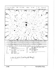
Figure 2.3: Schematic view of the wavelength coverage, dispersion directions, and image locations
for the FUSE detectors. In this figure, the detector pixel coordinates of the corner of each
segment are shown. The X, Y axes indicate orientation on the sky. Wavelength ranges shown
are approximate (see Table 2.2).
The SiC channels had an average dispersive plate scale of 1.03 ˚A/mm while the LiF channels
had a scale of 1.12 ˚A/mm (Moos et al. [2000]). Coupled with the detector pixel size, this resulted
in a scale of ∼6.7 m˚A/pixel in the LiF channel and ∼ 6.2 m˚A/pixel in the SiC channel (in the
X or dispersion direction).
The optical design of the FUSE spectrographs introduced astigmatism. The astigmatic
height of FUSE spectra perpendicular to the dispersion was significant; the dispersed image of
a point source had a vertical extent of 200 – 900 µm, or 14 – 63 ′′ , on the detector. An extended
source filling the large aperture was as large as 1200 µm, or 100 ′′ . This vertical astigmatic
height was a function of both wavelength and detector segment. This meant that the spatial
imaging capability of FUSE was extremely limited. For the spectral region near the minimum
astigmatic heights in each spectrum, there was marginal spatial information (> 10 ′′ ), but to
recover this requires careful, non-standard processing. The minimum astigmatic points were
near 1030 ˚A on the LiF channels and near 920 ˚A on the SiC channels.
Moreover, spectral features showed considerable curvature perpendicular to the dispersion,
especially near the ends of the detectors where the astigmatism was greatest. This astigmatism
is corrected for in the data prior to collapsing it into a 1-D spectrum (see Chapter 7 and the
Instrument Handbook (2009) for details).
6