
You also want an ePaper? Increase the reach of your titles
YUMPU automatically turns print PDFs into web optimized ePapers that Google loves.
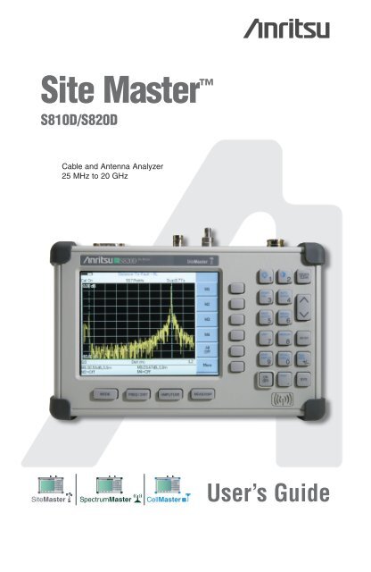
<strong>Site</strong> Master <br />
S810D/S820D<br />
Cable and Antenna Analyzer<br />
25 MHz to 20 GHz<br />
<strong>Site</strong><br />
Cell<br />
MS2712<br />
Master S331D <strong>Site</strong>Master MS2712<br />
SpectrumMaster<br />
Spectrum Master MS2711D Master MT8212A CellMaster<br />
MS2712<br />
<strong>Site</strong>Master SpectrumMaster CellMaster<br />
User’s Guide
WARRANTY<br />
The Anritsu product(s) listed on the title page is (are) warranted against defects in<br />
materials and workmanship for one year from the date of shipment.<br />
Anritsu's obligation covers repairing or replacing products which prove to be defective<br />
during the warranty period. Buyers shall prepay transportation charges for<br />
equipment returned to Anritsu for warranty repairs. Obligation is limited to the original<br />
purchaser. Anritsu is not liable for consequential damages.<br />
LIMITATION OF WARRANTY<br />
The foregoing warranty does not apply to Anritsu connectors that have failed due to<br />
normal wear. Also, the warranty does not apply to defects resulting from improper or<br />
inadequate maintenance by the Buyer, unauthorized modification or misuse, or operation<br />
outside the environmental specifications of the product. No other warranty is<br />
expressed or implied, and the remedies provided herein are the Buyer's sole and<br />
exclusive remedies.<br />
TRADEMARK ACKNOWLEDGMENTS<br />
Windows, Windows 95, Windows NT, Windows 98, Windows 2000, Windows ME<br />
and Windows XP are registered trademarks of the Microsoft Corporation.<br />
Anritsu, and <strong>Site</strong> Master are trademarks of Anritsu Company.<br />
NOTICE<br />
Anritsu Company has prepared this manual for use by Anritsu Company personnel<br />
and customers as a guide for the proper installation, operation and maintenance of<br />
Anritsu Company equipment and computer programs. The drawings, specifications,<br />
and information contained herein are the property of Anritsu Company, and any unauthorized<br />
use or disclosure of these drawings, specifications, and information is<br />
prohibited; they shall not be reproduced, copied, or used in whole or in part as the<br />
basis for manufacture or sale of the equipment or software programs without the<br />
prior written consent of Anritsu Company.<br />
UPDATES<br />
Updates to this manual, if any, may be downloaded from the Anritsu internet site at:<br />
http://www.us.anritsu.com.<br />
September 2006 10680-00001<br />
Copyright � 2005-2006 Anritsu Co. Revision: C
Table of Contents<br />
Chapter 1 - General Information<br />
Introduction . . . . . . . . . . . . . . . . . . . . . . . . . . . . . . . . . . 1-1<br />
Description . . . . . . . . . . . . . . . . . . . . . . . . . . . . . . . . . . . 1-1<br />
Options . . . . . . . . . . . . . . . . . . . . . . . . . . . . . . . . . . . . . 1-1<br />
Standard Accessories . . . . . . . . . . . . . . . . . . . . . . . . . . . . . 1-2<br />
Optional Accessories. . . . . . . . . . . . . . . . . . . . . . . . . . . . . . 1-2<br />
Option 5 Power Monitor Accessories . . . . . . . . . . . . . . . . . . . . . 1-3<br />
Coaxial Calibration Components . . . . . . . . . . . . . . . . . . . . . . . 1-3<br />
Coaxial Adapters. . . . . . . . . . . . . . . . . . . . . . . . . . . . . . . . 1-4<br />
Printers . . . . . . . . . . . . . . . . . . . . . . . . . . . . . . . . . . . . . 1-5<br />
Performance Specifications . . . . . . . . . . . . . . . . . . . . . . . . . . 1-6<br />
Preventive Maintenance . . . . . . . . . . . . . . . . . . . . . . . . . . . . 1-8<br />
Calibration . . . . . . . . . . . . . . . . . . . . . . . . . . . . . . . . . . . 1-8<br />
Annual Verification . . . . . . . . . . . . . . . . . . . . . . . . . . . . . . 1-9<br />
ESD Precautions . . . . . . . . . . . . . . . . . . . . . . . . . . . . . . . . 1-9<br />
Chapter 2 - Functions and Operations<br />
Introduction . . . . . . . . . . . . . . . . . . . . . . . . . . . . . . . . . . 2-1<br />
Test Connector Panel . . . . . . . . . . . . . . . . . . . . . . . . . . . . . 2-1<br />
Display Overview . . . . . . . . . . . . . . . . . . . . . . . . . . . . . . . 2-2<br />
Front Panel Overview . . . . . . . . . . . . . . . . . . . . . . . . . . . . . 2-3<br />
Function Hard Keys . . . . . . . . . . . . . . . . . . . . . . . . . . . . . . 2-4<br />
Keypad Hard Keys . . . . . . . . . . . . . . . . . . . . . . . . . . . . . . . 2-5<br />
Soft Keys. . . . . . . . . . . . . . . . . . . . . . . . . . . . . . . . . . . . 2-7<br />
Power Monitor Menus ............................2-17<br />
Symbols. ...................................2-18<br />
Self Test ...................................2-18<br />
Error Messages ................................2-19<br />
Battery Information. .............................2-22<br />
Charging a New Battery ..........................2-22<br />
Determining Remaining Battery Life. ...................2-24<br />
Important Battery Information .......................2-26<br />
Chapter 3 - Getting Started<br />
Introduction . . . . . . . . . . . . . . . . . . . . . . . . . . . . . . . . . . 3-1<br />
Power On Procedure . . . . . . . . . . . . . . . . . . . . . . . . . . . . . . 3-1<br />
CW Source Module Setup with Option 22 . . . . . . . . . . . . . . . . . . 3-2<br />
Cable and Antenna Analyzer Mode . . . . . . . . . . . . . . . . . . . . . . 3-2<br />
Save and Recall a Setup . . . . . . . . . . . . . . . . . . . . . . . . . . . 3-9<br />
Save and Recall a Display .........................3-10<br />
Changing the Units .............................3-10<br />
Changing the Language. ..........................3-10<br />
Adjusting Markers .............................3-11<br />
Adjusting Limits ..............................3-11<br />
i
ii<br />
Printing ....................................3-13<br />
Using the Soft Carrying Case. ........................3-14<br />
Chapter 4 - Cable and Antenna Analyzer Measurements<br />
Introduction . . . . . . . . . . . . . . . . . . . . . . . . . . . . . . . . . . 4-1<br />
Line Sweep Fundamentals . . . . . . . . . . . . . . . . . . . . . . . . . . . 4-1<br />
Fixed CW Mode . . . . . . . . . . . . . . . . . . . . . . . . . . . . . . . 4-2<br />
Information Required for a Line Sweep . . . . . . . . . . . . . . . . . . . 4-3<br />
Typical Line Sweep Test Procedures . . . . . . . . . . . . . . . . . . . . 4-3<br />
Chapter 5 - Power Measurement<br />
Introduction . . . . . . . . . . . . . . . . . . . . . . . . . . . . . . . . . . 5-1<br />
Power Measurement . . . . . . . . . . . . . . . . . . . . . . . . . . . . . . 5-1<br />
Chapter 6 - Handheld Software Tools<br />
Introduction . . . . . . . . . . . . . . . . . . . . . . . . . . . . . . . . . . 6-1<br />
Features . . . . . . . . . . . . . . . . . . . . . . . . . . . . . . . . . . . 6-1<br />
System Requirements . . . . . . . . . . . . . . . . . . . . . . . . . . . . . 6-1<br />
Installation . . . . . . . . . . . . . . . . . . . . . . . . . . . . . . . . . . . 6-2<br />
Using Handheld Software Tools . . . . . . . . . . . . . . . . . . . . . . . . 6-3<br />
Downloading Traces . . . . . . . . . . . . . . . . . . . . . . . . . . . . . 6-3<br />
Plot Capture to the PC . . . . . . . . . . . . . . . . . . . . . . . . . . . . 6-4<br />
Plot Upload to the Instrument . . . . . . . . . . . . . . . . . . . . . . . . 6-4<br />
Plot Properties . . . . . . . . . . . . . . . . . . . . . . . . . . . . . . . . 6-4<br />
Appendix A - Reference Data<br />
Coaxial Cable Technical Data. . . . . . . . . . . . . . . . . . . . . . . . . A-1<br />
Calibration Components. . . . . . . . . . . . . . . . . . . . . . . . . . . . A-5<br />
Waveguide-to-Coaxial Adapters . . . . . . . . . . . . . . . . . . . . . . . A-6<br />
Flange Compatibility . . . . . . . . . . . . . . . . . . . . . . . . . . . . . A-7<br />
Waveguide Technical Data .........................A-10<br />
Appendix B - Windowing<br />
Introduction . . . . . . . . . . . . . . . . . . . . . . . . . . . . . . . . . B-1<br />
Examples . . . . . . . . . . . . . . . . . . . . . . . . . . . . . . . . . . B-1<br />
Appendix C - Signal Standards<br />
Index<br />
Introduction . . . . . . . . . . . . . . . . . . . . . . . . . . . . . . . . . C-1
Introduction<br />
Chapter 1<br />
General Information<br />
This chapter provides a description, performance specifications, optional accessories, preventive<br />
maintenance, and calibration requirements for the <strong>Site</strong> Master models S810D and<br />
S820D. Throughout this manual, the term <strong>Site</strong> Master will refer to the S810D and S820D.<br />
Model Frequency Range<br />
S810D<br />
Cable and Antenna Analyzer: 0.025 to 10.5 GHz<br />
S820D<br />
Description<br />
Cable and Antenna Analyzer: 0.025 to 20 GHz<br />
The <strong>Site</strong> Master models S810D and S820D are hand held cable and antenna analyzers. Both<br />
models include a keypad to enter data and a thin film transistor liquid crystal display (TFT<br />
LCD) to provide graphic indications of various measurements.<br />
The <strong>Site</strong> Master is capable of up to 1.5 hours of continuous operation from a fully charged<br />
field-replaceable battery and can be operated from a 12.5 Vdc source. Built-in energy conservation<br />
features can be used to extend battery life.<br />
The <strong>Site</strong> Master is designed for measuring SWR, return loss, cable insertion loss and locating<br />
faulty RF components in antenna systems.<br />
The displayed trace can be scaled or enhanced with frequency markers or limit lines. A<br />
menu option provides for an audible “beep” when the limit value is exceeded. To permit<br />
use in low-light environments, the TFT LCD backlight intensity can be adjusted.<br />
Options<br />
Option 2 Low frequency extension (2 MHz low end frequency vs. standard 25<br />
MHz)<br />
Option 5 Power Monitor (sensor not included)<br />
Option 11NF Replaces standard K(f) Test Port Connector with N(f)<br />
Option 22NF 2-Port Cable-loss mode (Includes external N(f) CW source module<br />
CWM220NF, 560-7N50B detector, and 66379 adaptor cable.) Low Frequency<br />
Extension (2 MHz) and Power Monitor modes are enabled with<br />
this option.<br />
Option 22SF 2-Port Cable-loss mode (Includes external SMA (f) CW source module<br />
CWM220SF, 560-7S50B detector, and 66379 adaptor cable.) Low Frequency<br />
Extension (2 MHz) and Power Monitor modes are enabled with<br />
this option.<br />
Option 31 GPS Receiver (antenna included)<br />
1-1
Chapter 1 General Information<br />
Standard Accessories<br />
The following items are supplied with the <strong>Site</strong> Master:<br />
Part Number Description<br />
10680-00001 <strong>Site</strong> Master S810D/S820D User’s Guide<br />
48258 Soft Carrying Case<br />
633-27 Rechargeable NiMH Battery<br />
40-168 AC/DC Adapter<br />
806-141 Automotive Cigarette Lighter/12 Volt DC Adapter<br />
800-441 Serial Interface Cable (null modem type)<br />
2300-347 Anritsu Handheld Software Tools CDROM<br />
34RKNF50 Precision Adapter, Ruggedized K(m) to N(f)<br />
(not included when option 11NF is ordered)<br />
One year Warranty (includes battery, firmware, and software)<br />
The Handheld Software Tools PC-based software program provides a database record for<br />
storing measurement data. Software Tools can also convert the <strong>Site</strong> Master display to a<br />
Microsoft Windows� 95/98/NT4/2000/ME/XP workstation graphic. Measurements stored<br />
in the <strong>Site</strong> Master internal memory can be downloaded to the PC using the included<br />
null-modem serial cable. Once stored, the graphic trace can be displayed, scaled, or enhanced<br />
with markers and limit lines. Historical graphs can be overlaid with current data,<br />
and underlying data can be extracted and used in spreadsheets or for other analytical tasks.<br />
The Handheld Software Tools program can display measurements made with the <strong>Site</strong> Master<br />
(SWR, return loss, cable loss, distance-to-fault, field strength, occupied bandwidth,<br />
channel power, adjacent channel power and interference analysis) as well as providing<br />
other functions, such as converting display modes and Smith charts. Refer to Chapter 6,<br />
Handheld Software Tools, for more information.<br />
Optional Accessories<br />
The following optional accessories are available for the <strong>Site</strong> Master S8x0D:<br />
Part Number Description<br />
10680-00001 <strong>Site</strong> Master S810D/S820D User’s Guide<br />
10680-00002 <strong>Site</strong> Master S810D/S820D Programming Manual<br />
10680-00003 <strong>Site</strong> Master S810D/S820D Maintenance Manual<br />
2000-1410 Magnetic Mount GPS Antenna with 15 ft. cable<br />
48258 Soft Carrying Case<br />
760-213 Transit Case for Microwave <strong>Site</strong> Master<br />
40-168 AC/DC Adapter<br />
806-141 Automotive Cigarette Lighter/12 Volt DC Adapter<br />
633-27 Rechargeable NiMH Battery<br />
2000-1029 Battery Charger, External<br />
800-441 Serial Interface Cable (null modem type)<br />
551-1691 USB to RS232 Adapter Cable<br />
1-2
Option 5 Power Monitor Accessories<br />
Part Number Description<br />
560-7A50 Detector, 10 MHz to 18 GHz, GPC-7, 50 Ohm<br />
560-7N50B Detector, 10 MHz to 20 GHz, N(m), 50 Ohm<br />
560-7S50B Detector, 10 MHz to 20 GHz, WSMA(m), 50 Ohm<br />
560-7S50-2 Detector, 10 MHz to 26.5 GHz, WSMA(m), 50 Ohm<br />
560-7K50 Detector, 10 MHz to 40 GHz, K(m), 50 Ohm<br />
560-7VA50 Detector, 10 MHz to 50 GHz, V(m), 50 Ohm<br />
800-109 Detector Extender Cable, 7.6m (25 ft.)<br />
800-111 Detector Extender Cable, 30.5m (100 ft.)<br />
Coaxial Calibration Components<br />
K Connectors<br />
Part Number Description<br />
22K50 Precision K(m) Short/Open, 40 GHz<br />
22KF50 Precision K(f) Short/Open, 40 GHz<br />
28K50 Precision Termination, DC to 40 GHz, 50�, K(m)<br />
28KF50 Precision Termination, DC to 40 GHz, 50�, K(f)<br />
15KKF50-1.5A Armored Test Port Cable, 1.5 meter K(m) to K(f) 20 GHz<br />
15RKKF50-1.5A Ruggedized Armored Test Port Cable, 1.5 meter K(m) to K(f) 20 GHz<br />
OSLK50 Precision integrated Open/Short/Load K(m), DC to 20GHz, 50�<br />
N-Type Connectors<br />
Chapter 1 General Information<br />
Part Number Description<br />
22N50 Precision N(m) Short/Open, 18 GHz<br />
22NF50 Precision N(f) Short/Open, 18 GHz<br />
28N50-2 Precision Termination, DC to 18 GHz, 50�, N(m)<br />
28NF50-2 Precision Termination, DC to 18 GHz, 50�, N(f)<br />
15NNF50-1.5B Armored Test Port Cable, 1.5 meter N(m) to N(f) 18 GHz<br />
42N50-20 5W Attenuator, N(m) to N(f), 18 GHz<br />
OSLN50 Precision Integrated Open/Short/Load N(m), DC to 18GHz, 50�<br />
1-3
Chapter 1 General Information<br />
TNC Connectors<br />
Part Number Description<br />
1091-55 TNC Open (f), 18 GHz<br />
1091-53 TNC Open (m), 18 GHz<br />
1091-56 TNC Short (f), 18 GHz<br />
1091-54 TNC Short (m), 18 GHz<br />
1015-54 TNC Termination (f), 18 GHz<br />
1015-55 TNC Termination (m), 18 GHz<br />
Coaxial Adapters<br />
Part Number Description<br />
34NN50A Precision Adapter, DC to 18 GHz, N(m)-N(m), 50 Ohm<br />
34NFNF50 Precision Adapter, DC to 18 GHz, N(f) - N(f), 50 Ohm<br />
34RKNF50 Precision Ruggedized Adapter, K(m)-N(f), DC to 18 GHz, 50 Ohms<br />
34RSN50 Precision Ruggedized Adapter, WSMA(m)-N(m), DC to 18 GHz, 50 Ohms<br />
K220B Precision Adapter, DC to 40 GHz, 50 Ohm, K(m)-K(m)<br />
K222B Precision Adapter, DC to 40 GHz, 50 Ohm, K(f)-K(f)<br />
513-62 Adapter, DC to 18 GHz, TNC(f) to N(f), 50 Ohm<br />
1091-315 Adapter, DC to 18 GHz, TNC(m) to N(f), 50 Ohm<br />
1091-324 Adapter, DC to 18 GHz, TNC(f) to N(m), 50 Ohm<br />
1091-325 Adapter, DC to 18 GHz, TNC(m) to N(m), 50 Ohm<br />
1091-317 Adapter, DC to 18 GHz, TNC(m) to SMA(f), 50 Ohm<br />
1091-318 Adapter, DC to 18 GHz, TNC(m) to SMA(m), 50 Ohm<br />
1091-323 Adapter, DC to 18 GHz, TNC(m) to TNC(f), 50 Ohm<br />
1091-326 Adapter, DC to 18 GHz, TNC(m) to TNC(m), 50 Ohm<br />
1091-26 Adapter, DC to 18 GHz, N(m) - SMA(m), 50 Ohm<br />
1091-27 Adapter, DC to 18 GHz, N(m)-SMA(f), 50 Ohm<br />
1091-80 Adapter, DC to 18 GHz, 50 Ohm, N(f)-SMA(m)<br />
1091-81 Adapter, DC to 18 GHz, 50 Ohm, N(f)-SMA(f)<br />
1-4
Printers<br />
Chapter 1 General Information<br />
Part Number Description<br />
2000-1214 HP DeskJet Printer, Model 450. Includes printer cable, black print cartridge<br />
and U.S. power cord. Also includes serial-to-parallel Centronics converter cable<br />
and Centronics-to DB25 adapter. Rechargeable battery is optional and is<br />
not included.<br />
2000-1217 Rechargeable Battery for DeskJet Printer, Model 450<br />
2000-1216 Black Print Cartridge<br />
2000-753 Null Modem Serial-to-Parallel Centronics Converter Cable<br />
1091-310 Adapter 36-pin Centronics female-to-DB25 female<br />
2000-663 Power Cable (Europe) for DeskJet Printer<br />
2000-664 Power Cable (Australia) for DeskJet Printer<br />
2000-666 Power Cable (Japan) for DeskJet Printer<br />
2000-667 Power Cable (S. Africa) for DeskJet Printer<br />
2000-1218 Power Cable (U.K.) for DeskJet Printer<br />
1-5
Chapter 1 General Information<br />
Performance Specifications<br />
The specifications on the following pages describe the warranted performance of the instrument<br />
at 23°C ± 3°C when the unit is calibrated with the appropriate coaxial calibration kit<br />
for the built-in test port connector. A warm-up time of 15 minutes should be allowed prior<br />
to verifying system specifications. Performance parameters denoted as “typical” indicate<br />
non-warranted specifications.<br />
Frequency Range:<br />
<strong>Site</strong> Master S810D<br />
<strong>Site</strong> Master S820D<br />
Description Value<br />
0.025 to 10.5 GHz<br />
0.025 to 20.0 GHz<br />
Frequency Accuracy (Fixed CW ON) �3 ppm@25�C Frequency Resolution 10 kHz (100 kHz for Distance To Fault)<br />
Output Power (from RF Out port)
Description Value<br />
Test Port Connector Precision K(f) or N(f) (Option 11NF)<br />
Language Support English, Spanish, French, German, Chinese, Japanese<br />
Internal Trace Memory Up to 200 traces<br />
Setup Configuration 21<br />
Custom Cable Configuration Memory up to 200 configurations<br />
Display TFT color display with adjustable backlight<br />
Ports<br />
CE<br />
Environmental<br />
(MIL-PRF- 28800F<br />
Class 2)<br />
RF Out:<br />
Serial Interface:<br />
Electromagnetic<br />
Compatibility:<br />
Safety:<br />
Temperature/Humidity:<br />
Mechanical:<br />
Standard: Type K(f) test port, 50� +23 dBm<br />
(Peak), ±50 VDC, Maximum input without damage<br />
Optional (S8x0D/11NF): Type N(f) test port, 50�<br />
+23 dBm (Peak), ±50 VDC, Maximum input without<br />
damage<br />
9 pin D-sub RS-232 three wire serial<br />
Meets European Community requirement<br />
EN61326-1:1998<br />
Meets European Community requirement<br />
EN61010-1:2001<br />
Operating: –10ºC to 55ºC, humidity 85% or less<br />
Non-operating: –51ºC to +71ºC (recommend storing<br />
the battery separately between 0ºC and +40ºC<br />
for any prolonged non-operating storage period)<br />
Vibration: Sine (5-55 Hz); Random (10-500 Hz)<br />
Shock: 30 G, 11 msec, half sine<br />
Power Supply External:<br />
DC input: +12 to +15 volt dc, 3A<br />
Internal: NiMH battery: 10.8 volts, 1800 mAh<br />
Dimensions<br />
Size (W xHxD):<br />
Weight:<br />
25.4 cm x 17.8 cm x 6.1 cm<br />
(10.0 in x 7.0 in x 2.4 in)<br />
Chapter 1 General Information<br />
Low Frequency<br />
Extension<br />
(S8X0D/2)<br />
Description Value<br />
2-Port Cable Loss (S8X0D/22XF)<br />
CW Source Module<br />
(CWM220xF)<br />
2- Port Cable Loss<br />
Measurement<br />
Frequency Range:<br />
Frequency Range<br />
Freq Accuracy ±3ppm @ 25� C<br />
Power at RF Out<br />
Port<br />
Ports<br />
2 MHz to 20000 MHz (S820D)<br />
2 MHz to 10500 MHz (S810D)<br />
(All other specs remain the same as the standard<br />
S8x0D.)<br />
2 MHz to 20000 MHz (with S820D)<br />
2 MHz to 10500 MHz (with S810D)<br />
+15dBm, maximum (typically > -10dBm)<br />
CWM220NF: N(f), ±15 VDC, +20 dBm, maximum<br />
input, no damage<br />
CWM220SF: SMA(f), ±15 VDC, +20 dBm, maximum<br />
input, no damage<br />
Detector Range -50 to +20 dBm, 10 nW to 100 mW<br />
Display Range -60 to +60 dB(m)<br />
Resolution 0.1 dB<br />
Measurement<br />
Accuracy (following<br />
a calibration)<br />
Preventive Maintenance<br />
±0.85 dB, maximum for < 10 dB cable loss<br />
±1.35 dB, maximum for < 30 dB cable loss<br />
(using 560-7S50B from 10MHz to 20GHz<br />
or 560-7N50B from 10MHz to 18 GHz)<br />
<strong>Site</strong> Master preventive maintenance consists of cleaning the unit and inspecting and cleaning<br />
the RF connectors on the instrument and all accessories. Clean the <strong>Site</strong> Master with a<br />
soft, lint-free cloth dampened with water or water and a mild cleaning solution.<br />
CAUTION: To avoid damaging the display or case, do not use solvents or abrasive<br />
cleaners.<br />
Clean the RF connectors and center pins with a cotton swab dampened with denatured alcohol.<br />
Visually inspect the connectors. The fingers and pins of the connectors should be unbroken<br />
and uniform in appearance. If you are unsure whether the connectors are good,<br />
gauge the connectors to confirm that the dimensions are correct. Visually inspect the test<br />
port cable(s). The test port cable should be uniform in appearance, not stretched, kinked,<br />
dented, or broken.<br />
Calibration<br />
The <strong>Site</strong> Master is a field portable unit operating in the rigors of the test environment. An<br />
Open-Short-Load (OSL) calibration should be performed prior to making a measurement in<br />
the field (see Calibration, page 3-3). A built-in temperature sensor in the <strong>Site</strong> Master advises<br />
the user when the internal temperature has exceeded a measurement accuracy window,<br />
and the user is advised to perform another calibration in order to maintain the integrity<br />
of the measurement.<br />
1-8
NOTES:<br />
For best calibration results—compensation for all measurement uncertainties—ensure<br />
that the Open/Short/Load is at the end of the test port or optional<br />
extension cable; that is, at the same point that you will connect the antenna or<br />
device to be tested.<br />
For best results, use a phase stable Test Port Extension Cable (see Optional<br />
Accessories). If you use a typical laboratory cable to extend the <strong>Site</strong> Master test<br />
port to the device under test, cable bending subsequent to the OSL calibration<br />
will cause uncompensated phase reflections inside the cable. Thus, cables<br />
which are NOT phase stable may cause measurement errors that are more pronounced<br />
as the test frequency increases.<br />
For optimum calibration, Anritsu recommends using precision calibration components.<br />
Annual Verification<br />
Anritsu recommends an annual calibration and performance verification of the <strong>Site</strong> Master<br />
and the OSL calibration components by local Anritsu service centers. Anritsu service centers<br />
are listed in Table 1-2 on the following page.<br />
The <strong>Site</strong> Master itself is self-calibrating, meaning that there are no field-adjustable components.<br />
However, the OSL calibration components are crucial to the integrity of the calibration<br />
and therefore, must be verified periodically to ensure performance conformity. This is<br />
especially important if the OSL calibration components have been accidentally dropped or<br />
over-torqued.<br />
ESD Precautions<br />
Chapter 1 General Information<br />
The <strong>Site</strong> Master, like other high performance instruments, is susceptible to ESD damage.<br />
Very often, coaxial cables and antennas build up a static charge, which, if allowed to discharge<br />
by connecting to the <strong>Site</strong> Master, may damage the <strong>Site</strong> Master input circuitry. <strong>Site</strong><br />
Master operators should be aware of the potential for ESD damage and take all necessary<br />
precautions. Operators should exercise practices outlined within industry standards like<br />
JEDEC-625 (EIA-625), MIL-HDBK-263, and MIL-STD-1686, which pertain to ESD and<br />
ESDS devices, equipment, and practices.<br />
As these apply to the <strong>Site</strong> Master, it is recommended to dissipate any static charges that<br />
may be present before connecting the coaxial cables or antennas to the <strong>Site</strong> Master. This<br />
may be as simple as temporarily attaching a short or load device to the cable or antenna<br />
prior to attaching to the <strong>Site</strong> Master. It is important to remember that the operator may also<br />
carry a static charge that can cause damage. Following the practices outlined in the above<br />
standards will insure a safe environment for both personnel and equipment.<br />
1-9
Chapter 1 General Information<br />
Table 1-3. Anritsu Service Centers<br />
UNITED STATES<br />
ANRITSU COMPANY<br />
490 Jarvis Drive<br />
Morgan Hill, CA 95037-2809<br />
Telephone: (408) 776-8300<br />
1-800-ANRITSU<br />
FAX: 408-776-1744<br />
ANRITSU COMPANY<br />
10 New Maple Ave., Unit 305<br />
Pine Brook, NJ 07058<br />
Telephone: (973) 227-8999<br />
1-800-ANRITSU<br />
FAX: 973-575-0092<br />
ANRITSU COMPANY<br />
1155 E. Collins Blvd<br />
Richardson, TX 75081<br />
Telephone: 1-800-ANRITSU<br />
FAX: 972-671-1877<br />
AUSTRALIA<br />
ANRITSU PTY. LTD.<br />
Unit 3, 170 Foster Road<br />
Mt Waverley, VIC 3149<br />
Australia<br />
Telephone: 03-9558-8177<br />
FAX: 03-9558-8255<br />
BRAZIL<br />
ANRITSU ELECTRONICA LTDA.<br />
Praça Amadeu Amaral 27, 1º andar.<br />
Bela Vista, São Paulo, SP, Brasil<br />
CEP: 01327-010<br />
Telephone: 55-11-3283-2511<br />
Fax: 55-11-3288-6940<br />
CANADA<br />
ANRITSU INSTRUMENTS LTD.<br />
700 Silver Seven Road, Suite 120<br />
Kanata, Ontario K2V 1C3<br />
Telephone: (613) 591-2003<br />
FAX: (613) 591-1006<br />
CHINA<br />
ANRITSU ELECTRONICS (SHANGHAI)<br />
CO. LTD.<br />
2F, Rm B, 52 Section Factory Building<br />
No. 516 Fu Te Rd (N)<br />
Shanghai 200131 P.R. China<br />
Telephone:21-58680226, 58680227,<br />
58680228<br />
FAX: 21-58680588<br />
1-10<br />
FRANCE<br />
ANRITSU S.A<br />
9 Avenue du Quebec<br />
Zone de Courtaboeuf<br />
91951 Les Ulis Cedex<br />
Telephone: 016-09-21-550<br />
FAX: 016-44-61-065<br />
GERMANY<br />
ANRITSU GmbH<br />
Grafenberger Allee 54-56<br />
D-40237 Dusseldorf, Germany<br />
Telephone: 0211-968550<br />
FAX: 0211-9685555<br />
INDIA<br />
MEERA AGENCIES PVT. LTD.<br />
23 Community Centre<br />
Zamroodpur, Kailash Colony Extension,<br />
New Delhi, India 110 048<br />
Phone: 011-2-6442700/6442800<br />
FAX : 011-2-644250023<br />
ISRAEL<br />
TECH-CENT, LTD.<br />
4 Raul Valenberg St<br />
Tel-Aviv 69719<br />
Telephone: (03) 64-78-563<br />
FAX: (03) 64-78-334<br />
ITALY<br />
ANRITSU Sp.A<br />
Roma Office<br />
Via E. Vittorini, 129<br />
00144 Roma EUR<br />
Telephone: (06) 50-99-711<br />
FAX: (06) 50-22-4252<br />
JAPAN<br />
ANRITSU CUSTOMER SERVICE LTD.<br />
5-1-1 Onna, Atsugi-shi<br />
Kanagawa, 243-8555 Japan<br />
Telephone: 0462-96-6688<br />
FAX: 0462-25-8379<br />
KOREA<br />
ANRITSU CORPORATION LTD.<br />
Service Center:<br />
8F Hyunjuk Building<br />
832-41, Yeoksam Dong<br />
Kangnam-Gu<br />
Seoul, South Korea 135-080<br />
Telephone: 82-2-553-6603<br />
FAX: 82-2-553-6605<br />
SINGAPORE<br />
ANRITSU (SINGAPORE) PTE LTD.<br />
10, Hoe Chiang Road<br />
#07-01/02 Keppel Towers<br />
Singapore 089315<br />
Telephone: 282-2400<br />
FAX: 282-2533<br />
SOUTH AFRICA<br />
ETECSA<br />
12 Surrey Square Office Park<br />
330 Surrey Avenue<br />
Ferndale, Randburt, 2194<br />
South Africa<br />
Telephone: 011-27-11-787-7200<br />
FAX: 011-27-11-787-0446<br />
SWEDEN<br />
ANRITSU AB<br />
Fagelviksvagen 9A<br />
145 84 Stockholmn<br />
Telephone: (08) 534-707-00<br />
FAX: (08) 534-707-30<br />
TAIWAN<br />
ANRITSU CO., INC.<br />
7F, No. 316, Section 1<br />
NeiHu Road<br />
Taipei, Taiwan, R.O.C.<br />
Telephone: 886-2-8751-1816<br />
FAX: 886-2-8751-2126<br />
UNITED KINGDOM<br />
ANRITSU LTD.<br />
200 Capability Green<br />
Luton, Bedfordshire<br />
LU1 3LU, England<br />
Telephone: 015-82-433200<br />
FAX: 015-82-731303
Introduction<br />
Chapter 2<br />
Functions and Operations<br />
This chapter provides a brief overview of the <strong>Site</strong> Master functions and operations, providing<br />
the user with a starting point for making basic measurements. For more detailed information,<br />
refer to the specific chapters for the measurements being made.<br />
The <strong>Site</strong> Master is designed specifically for field environments and applications requiring<br />
mobility. As such, it is a lightweight, handheld, battery operated unit which can be easily<br />
carried to any location, and is capable of up to 1.5 hours of continuous operation from a<br />
field replaceable battery for extended time in the field. Built-in energy conservation features<br />
allow battery life to be further extended. The <strong>Site</strong> Master can also be powered by a<br />
12.5 Vdc external source. The external source can be either the Anritsu AC-DC Adapter<br />
(P/N 40-168) or 12.5 Vdc Automotive Cigarette Lighter Adapter (P/N 806-141). Both items<br />
are standard accessories.<br />
Test Connector Panel<br />
12-15 VDC<br />
(3A)<br />
The connectors and indicators located on the test panel (Figure 2-1) are listed and described<br />
below.<br />
EXTERNAL POWER RF OUT/REFLECTION<br />
BATTERY<br />
CHARGING LED<br />
SERIAL<br />
INTERFACE<br />
Figure 2-1. S8x0D Test Connector Panel<br />
GPS ANTENNA<br />
EXTERNAL POWER LED<br />
12 to 15 Vdc @ 3A input to power the unit or for battery charging.<br />
WARNING<br />
RF DETECTOR INPUT (OPTION 5)<br />
CW SOURCE MODULE<br />
INTERFACE (OPTION 22)<br />
When using the AC-DC Adapter, always use a three-wire power cable connected<br />
to a three-wire power line outlet. If power is supplied without grounding the equipment<br />
in this manner, there is a risk of receiving a severe or fatal electric shock, or<br />
damaging the equipment.<br />
2-1
Chapter 2 Functions and Operations<br />
Battery<br />
Charging<br />
External<br />
Power<br />
Serial<br />
Interface<br />
Illuminates when the battery is being charged. The indicator automatically shuts<br />
off when the battery is fully charged.<br />
Illuminates when the <strong>Site</strong> Master is being powered by the external charging unit.<br />
RS232 DB9 interface to a COM port on a personal computer (for use with the<br />
Anritsu Handheld Software Tools program) or to a supported printer.<br />
RF Out/ RF output, 50 � impedance, for reflection measurements. Maximum input is<br />
Reflection 50� +23 dBm at �50 Vdc.<br />
GPS Antenna GPS antenna connection. Do not connect anything other than the Anritsu GPS<br />
antenna to this port.<br />
Display Overview<br />
2-2<br />
Figure 2-2 illustrates some of the key information areas of the S8x0D display.<br />
CALIBRATION<br />
STATUS<br />
DATA<br />
POINTS<br />
Figure 2-2. S8x0D Display Overview<br />
MESSAGEAREA<br />
TITLE BAR<br />
SWEEP<br />
TIME<br />
CURRENT<br />
MENU
Front Panel Overview<br />
The <strong>Site</strong> Master menu-driven user interface is easy to use and requires little training. Hard<br />
keys on the front panel are used to initiate function-specific menus. There are four function<br />
hard keys located below the status window: Mode, Frequency/Distance, Amplitude and<br />
Measure/Display.<br />
There are seventeen keypad hard keys located to the right of the status window. Twelve of<br />
the keypad hard keys perform more than one function, depending on the current mode of<br />
operation. The dual purpose keys are labeled with one function in black, the other in blue.<br />
There are also six soft keys that change function depending upon the current mode selection.<br />
The current soft key function is indicated in the soft key menu area to the right of the<br />
status window. The locations of the different keys are illustrated in Figure 2-3.<br />
Soft Key<br />
Menu<br />
Status Window<br />
MODE FREQ/DIST AMPLITUDE MEAS/DISP<br />
Function Hard Keys<br />
Figure 2-3. <strong>Site</strong> Master Front Panel<br />
S820D <strong>Site</strong>Master<br />
START<br />
CAL<br />
3<br />
SAVE<br />
SETUP<br />
SAVE<br />
DISPLAY<br />
The following sections describe the various key functions.<br />
Chapter 2 Functions and Operations<br />
Soft Keys<br />
AUTO<br />
SCALE<br />
4<br />
RECALL<br />
SETUP<br />
LIMIT MARKER<br />
7 8<br />
ENTER<br />
ON<br />
OFF<br />
1 2<br />
5 6<br />
RECALL<br />
DISPLAY<br />
9 0<br />
PRINT<br />
.<br />
ESCAPE<br />
CLEAR<br />
RUN<br />
HOLD<br />
+ / -<br />
SYS<br />
Keypad<br />
Hard<br />
Keys<br />
2-3
Chapter 2 Functions and Operations<br />
Function Hard Keys<br />
MODE Opens the mode selection box (below). Use the Up/Down arrow key to select a<br />
mode. Press the ENTER key to implement.<br />
NOTE: Available mode selections will vary according to model number and options<br />
installed.<br />
FREQ/DIST Displays the Frequency or Distance to Fault soft key menus depending on the<br />
measurement mode (see page 2-11).<br />
AMPLITUDE Displays the amplitude soft key menu for the current operating mode (see page<br />
2-12).<br />
MEAS/DISP Displays the measurement and display soft key menus for the current operating<br />
mode (see page 2-12).<br />
2-4<br />
� Measurement Mode<br />
Freq - SWR<br />
Figure 2-4. Mode Selection Box<br />
Return Loss<br />
Cable Loss - One Port<br />
Cable Loss - Two Port<br />
DTF - SWR<br />
Return Loss<br />
Power Monitor
Keypad Hard Keys<br />
This section contains an alphabetical listing of the <strong>Site</strong> Master front panel keypad controls<br />
along with a brief description of each. More detailed descriptions of the major function<br />
keys follow.<br />
The following keypad hard key functions are printed in black on the keypad keys.<br />
0-9 These keys are used to enter numerical data as required to setup or perform<br />
measurements.<br />
+/–<br />
The plus/minus key is used to enter positive or negative values as required<br />
to setup or perform measurements.<br />
� The decimal point is used to enter decimal values as required to setup or<br />
perform measurements.<br />
ESCAPE<br />
CLEAR<br />
Up/Down<br />
Arrows<br />
Exits the present operation or clears the status window. If a parameter is<br />
being edited, pressing this key will clear the value currently being entered<br />
and restore the last valid entry. Pressing this key again will close the parameter.<br />
During normal sweeping, pressing this key will move up one<br />
menu level.<br />
Increments or decrements a parameter value. The specific parameter value<br />
affected typically appears in the message area of the LCD.<br />
ENTER Implements the current action or parameter selection.<br />
ON<br />
OFF<br />
Chapter 2 Functions and Operations<br />
Turns the Anritsu <strong>Site</strong> Master on or off. When turned on, the saved system<br />
state at the last turn-off is restored. If the ESCAPE/CLEAR key is held<br />
down while the ON/OFF key is pressed, the factory preset state will be<br />
restored.<br />
SYS Allows selection of the system setup parameters and display language. In<br />
cable and antenna analyzer modes, the choices are Options, Clock, Self<br />
Test, Status and Language.<br />
2-5
Chapter 2 Functions and Operations<br />
2-6<br />
The following keypad hard key functions are printed in blue on the keypad keys.<br />
This key is used to adust the brightness of the color display. Use the<br />
Up/Down arrow key and ENTER to adjust the display brightness.<br />
AUTO<br />
SCALE<br />
Automatically scales the status window for optimum resolution in cable<br />
and antenna analyzer mode.<br />
LIMIT Displays the limit line menu for the current operating mode when in cable<br />
or antenna analyzer mode.<br />
MARKER Displays the marker menu of the current operating mode when in cable or<br />
antenna analyzer mode.<br />
PRINT Prints the current display to the selected printer via the RS232 serial port.<br />
RECALL<br />
DISPLAY<br />
RECALL<br />
SETUP<br />
RUN<br />
HOLD<br />
SAVE<br />
DISPLAY<br />
SAVE<br />
SETUP<br />
START<br />
CAL<br />
Recalls a previously saved trace from memory. When the key is pressed, a<br />
Recall Trace selection box appears on the display. Select a trace using the<br />
Up/Down arrow key and press the ENTER key to implement.<br />
Recalls a previously saved setup from a memory location. When the key<br />
is pressed, a Recall Setup selection box appears on the display. Select a<br />
setup using the Up/Down arrow key and press the ENTER key to implement.<br />
Setup 0 recalls the factory preset state for the current mode.<br />
When in the Hold mode, this key starts the <strong>Site</strong> Master sweeping and provides<br />
a Single Sweep Mode trigger; when in the Run mode, it pauses the<br />
sweep. When in the Hold mode, the hold symbol (page 2-18) appears on<br />
the display. Hold mode can be used to conserve battery power.<br />
Saves up to 200 displayed traces to non-volatile memory. When the key is<br />
pressed, the Trace Name: box appears. Use the soft keys to enter up to 16<br />
alphanumeric characters for that trace name and press the ENTER key to<br />
save the trace.<br />
Saves the current system setup to an internal non-volatile memory location.<br />
The number of locations available varies with the model number and<br />
installed options. There are ten available locations in cable and antenna<br />
analyzer mode and five in Power Monitor mode (Option 5). When the key<br />
is pressed, a Save Setup selection box appears on the status window. Use<br />
the Up/Down arrow key to select a setup and press the ENTER key to implement.<br />
Starts the calibration in SWR, Return Loss, Cable Loss, or DTF measurement<br />
modes (not available in Power Monitor mode).
Soft Keys<br />
Each keypad key opens a set of soft key selections. Each of the soft keys has a corresponding<br />
soft key label area on the status window. The label identifies the function of the soft key<br />
for the current Mode selection.<br />
The following figures show the soft key labels for each Mode selection.<br />
MODE=FREQ:<br />
SOFTKEYS: F1<br />
Top<br />
of<br />
List<br />
Page Up<br />
Page<br />
Down<br />
Bottom<br />
of<br />
List<br />
FREQ/DIST AMPLITUDE MEAS/DISP<br />
F2<br />
Signal<br />
Standard<br />
Figure 2-5. Return Loss Mode Soft Key Labels<br />
Top<br />
Bottom<br />
Top<br />
of<br />
List<br />
Page Up<br />
Page<br />
Down<br />
Bottom<br />
of<br />
List<br />
Delete<br />
Trace<br />
Delete<br />
All<br />
Trace<br />
On/Off<br />
Select<br />
Trace<br />
Back<br />
Chapter 2 Functions and Operations<br />
*<br />
Resolution<br />
Single<br />
Sweep<br />
Trace<br />
Math<br />
Trace<br />
Overlay<br />
Fixed<br />
CW<br />
Smoothing<br />
130<br />
259<br />
517<br />
* Fixed CW is not available in Cable Loss - Two Port mode.<br />
2-7
Chapter 2 Functions and Operations<br />
2-8<br />
MODE=DTF:<br />
SOFTKEYS:<br />
with Waveguide<br />
Calibration<br />
Waveguide<br />
Loss<br />
Cutoff<br />
Freq<br />
Waveguide<br />
Window<br />
Back<br />
with Coaxial<br />
Calibration<br />
Loss<br />
Prop<br />
Vel<br />
Cable<br />
Window<br />
Back<br />
FREQ/DIST AMPLITUDE<br />
D1<br />
D2<br />
DTF Aid<br />
More<br />
Figure 2-6. Distance to Fault Mode Soft Key Labels<br />
Top<br />
Bottom<br />
Top<br />
of<br />
List<br />
Page Up<br />
Page<br />
Down<br />
Bottom<br />
of<br />
List<br />
Delete<br />
Trace<br />
Delete<br />
All<br />
Traces<br />
On/Off<br />
Select<br />
Trace<br />
Back<br />
MEAS/DISP<br />
Resolution<br />
Single<br />
Sweep<br />
Trace<br />
Math<br />
Trace<br />
Overlay<br />
Fixed<br />
CW
MODE=POWER MONITOR:<br />
SOFTKEYS:<br />
Figure 2-7. Power Monitor Mode Soft Key Labels (Option 5)<br />
GPS<br />
On/Off<br />
Location<br />
Quality<br />
Reset<br />
Back<br />
Units<br />
Printer<br />
Change<br />
Date<br />
Format<br />
GPS<br />
Back<br />
Options<br />
Clock<br />
Self<br />
Test<br />
Status<br />
Language<br />
English<br />
Figure 2-8. SYS Key Menu in Cable and Antenna Analyzer Mode<br />
Chapter 2 Functions and Operations<br />
AMPLITUDE<br />
Units<br />
Rel<br />
Offset<br />
dB<br />
Zero<br />
Hour<br />
Minute<br />
Month<br />
Day<br />
Year<br />
Back<br />
2-9
Chapter 2 Functions and Operations<br />
2-10<br />
GPS<br />
On/Off<br />
Location<br />
Quality<br />
Reset<br />
Back<br />
Printer<br />
Change<br />
Date<br />
Format<br />
GPS<br />
Back<br />
Figure 2-9. SYS Key Menu in Power Monitor Mode<br />
Options<br />
Clock<br />
Self<br />
Test<br />
Status<br />
Language<br />
English<br />
Hour<br />
Minute<br />
Month<br />
Day<br />
Year<br />
Back
FREQ/DIST Displays the frequency and distance menu depending on the measurement mode.<br />
Frequency<br />
Menu<br />
Distance<br />
Menu<br />
Distance<br />
Sub-Menu<br />
(Waveguide)<br />
The frequency and distance menu for cable and antenna analyzer measurements<br />
provides for setting sweep frequency end points when Freq mode is selected. Selected<br />
frequency values may be changed using the keypad or Up/Down arrow<br />
key.<br />
� F1 — Opens the F1 parameter for data entry. This is the start value for the<br />
frequency sweep. Press ENTER when data entry is complete.<br />
� F2 — Opens the F2 parameter for data entry. This is the stop value for the<br />
frequency sweep. Press ENTER when data entry is complete.<br />
� Signal Standard — Allows selection of the signal standard to be used. Select<br />
from the available international standards (Appendix C).<br />
Provides for setting Distance to Fault parameters when a DTF mode is selected.<br />
Choosing DIST causes the soft keys, below, to be displayed and the corresponding<br />
values to be shown in the message area. Selected distance values may be<br />
changed using the keypad or Up/Down arrow key.<br />
� D1 — Opens the start distance (D1) parameter for data entry. This is the start<br />
value for the distance range (D1 default = 0). Press ENTER when data entry<br />
is complete.<br />
� D2 — Opens the end distance (D2) parameter for data entry. This is the end<br />
value for the distance range. Press ENTER when data entry is complete.<br />
� DTF Aid — Provides interactive help to optimize DTF set up parameters. Use<br />
the Up/Down arrow key to select a parameter to edit. Press ENTER when<br />
data entry is complete.<br />
� More — Selects one of the Distance Sub-Menus, detailed below, depending<br />
on whether the current calibration is for coaxial cable or wavguide media.<br />
Provides for setting the waveguide loss and cutoff frequency parameters of the<br />
waveguide. Selected values may be changed using the Up/Down arrow key or<br />
keypad.<br />
� Waveguide Loss — Opens the Waveguide Loss parameter for data entry. Enter<br />
the loss per meter (or foot) for the type of transmission line being tested.<br />
Press ENTER when data entry is complete. (Range is 0 to 5.000 dB/m.)<br />
� Cutoff Freq — Opens the cutoff frequency parameter for data entry. Enter the<br />
cutoff frequency for the type of waveguide being tested. Press ENTER when<br />
data entry is complete. (Range is 0 to 20)<br />
� Waveguide — Opens the waveguide list showing the currently selected<br />
waveguides. Highlight the desired waveguide and use the Up/Down arrow<br />
key and ENTER to make a selection. Press the Show All soft key to show the<br />
complete waveguide list, where the currently selected waveguides are marked<br />
with an asterisk. Press the Show Selected soft key to show only the selected<br />
waveguides.<br />
� Window — Opens a menu of FFT windowing types for the DTF calculation.<br />
Scroll the menu using the Up/Down arrow key and make a selection with the<br />
ENTER key.<br />
� Back — Returns to the Distance Menu.<br />
Chapter 2 Functions and Operations<br />
2-11
Chapter 2 Functions and Operations<br />
Distance<br />
Sub-Menu<br />
(Coax Cable)<br />
Provides for setting the cable loss and relative propagation velocity of the coaxial<br />
cable. Selected values may be changed using the Up/Down arrow key or keypad.<br />
� Loss — Opens the Cable Loss parameter for data entry. Enter the loss per<br />
meter (or foot) for the type of transmission line being tested. Press<br />
ENTER when data entry is complete. (Range is 0 to 5.0 dB/m)<br />
� Prop Vel (relative propagation velocity) — Opens the Propagation Velocity<br />
parameter for data entry. Enter the propagation velocity for the type of<br />
transmission line being tested. Press ENTER when data entry is complete.<br />
(Range is 0.010 to 1.000)<br />
� Cable — Opens the coaxial cable list showing the currently selected coaxial<br />
cables. Highlight the desired coaxial cable and use the Up/Down arrow<br />
key and ENTER to make a selection. Press the Show All soft key to<br />
show the complete coaxial cable list, where the currently selected coaxial<br />
cables are marked with an asterisk. Press the Show Selected soft key to<br />
show only the selected coaxial cables.<br />
This feature provides a rapid means of setting both cable loss and propagation<br />
velocity. (Refer to Appendix A for a listing of common coaxial cables<br />
showing values for Relative Propagation Velocity and Nominal<br />
Attenuation in dB/m at the frequencies listed.) When a cable is selected<br />
the nominal attenuation will be set to the value associated with the frequency<br />
in the table that is closest to the mid band of the frequency range<br />
for the measurement. Custom coaxial cables can be uploaded via the<br />
Handheld Software Tools program.<br />
� Window — Opens a menu of FFT windowing types for the DTF calculation.<br />
Scroll the menu using the Up/Down arrow key and make a selection<br />
with the ENTER key. Refer to Appendix B for more details on windowing.<br />
� Back — Returns to the Distance Menu.<br />
AMPLITUDE Displays the amplitude or scale menu depending on the measurement mode.<br />
Amplitude<br />
Menu<br />
Provides for changing the status window scale. Selected values may be changed<br />
using the Up/Down arrow key or keypad.<br />
Choosing AMPLITUDE in cable and antenna analyzer measurement modes<br />
causes the soft keys, below, to be displayed and the corresponding values to be<br />
shown in the message area.<br />
� Top — Opens the top parameter for data entry and provides for setting the<br />
top scale value. Press ENTER when data entry is complete.<br />
� Bottom — Opens the bottom parameter for data entry and provides for setting<br />
the bottom scale value. Press ENTER when data entry is complete.<br />
MEAS/DISP Displays the Meas/Disp soft key menu for the current operating mode.<br />
Meas/Disp<br />
Menu<br />
2-12<br />
Provides for changing the status window resolution, single or continuous sweep,<br />
and access to the Trace Math functions.<br />
Choosing MEAS/DISP in cable and antenna analyzer Freq or DTF measurement<br />
modes causes the soft keys below to be displayed.
Chapter 2 Functions and Operations<br />
� Resolution — Opens the status window to change the resolution. Choose 130,<br />
259, or 517 data points. (In DTF mode, resolution can only be adjusted<br />
through the DTF Aid table.)<br />
� Single Sweep — Toggles the sweep between single sweep and continuous<br />
sweep. In single sweep mode, each sweep must be activated by the<br />
RUN/HOLD button.<br />
� Trace Math — Opens up the Trace Math functions (trace-memory or<br />
trace+memory) for comparison of the real time trace in the status window<br />
with any of the traces from memory. (Not available in DTF mode.)<br />
� Trace Overlay — Opens up the Trace Overlay functions menu to allow the<br />
current trace to be displayed with a trace in memory overlaid on it. Choose<br />
On or Off and Select Trace to select the trace from memory to be overlaid.<br />
� Fixed CW — Toggles the fixed CW function ON or OFF. When OFF, a narrow<br />
band of frequencies around the selected frequency is generated. This enhances<br />
the immunity of the <strong>Site</strong> Master to an interfering signal. When CW is<br />
ON, only a single frequency with a very narrow band width is generated by<br />
the <strong>Site</strong> Master. The sweep speed is faster in CW ON mode. If CW is ON<br />
during normal RL or SWR measurements, it may be more susceptible to interfering<br />
signals, so use this feature with caution. Interfering signals can<br />
make the measurement look better or worse than it really is.<br />
� Smoothing — Sets the level of smoothing applied to a frequency measurement<br />
trace. A level of 0 turns smoothing OFF. Levels 1 through 20 turn<br />
smoothing ON and set the smoothing percentage (the higher the level, the<br />
higher the smoothing applied to the trace). Smoothing is a trace averaging<br />
process that reduces or removes ripples from frequency swept data. This is<br />
especially useful when making 1-port cable loss measurements with a short at<br />
the other end of the cable. The ripple that is usually present in this kind of<br />
measurement can be removed with smoothing resulting in a more accurate<br />
average cable loss frequency response trace. Care should be taken when applying<br />
smoothing so as not to remove ripples that are inherent parts of the<br />
data (as opposed to measurement artifacts).<br />
MARKER Choosing MARKER in cable and antenna analyzer freq and dist mode causes<br />
the soft keys, below, to be displayed and the corresponding values to be shown<br />
in the message area. Selected frequency marker or distance marker locations<br />
may be changed using the keypad or Up/Down arrow key.<br />
� M1 — Selects the M1 marker parameter and opens the M1 marker second<br />
level menu.<br />
� On/Off — Turns the selected marker on or off.<br />
� Edit — Opens the selected marker parameter for data entry. Press<br />
ENTER when data entry is complete or ESCAPE to restore the previous<br />
value.<br />
� Marker To Peak — Places the selected marker at the frequency or distance<br />
with the maximum amplitude value.<br />
� Marker To Valley — Places the selected marker at the frequency or distance<br />
with the minimum amplitude value.<br />
� Back — Returns to the Main Markers Menu.<br />
� M2 through M4 — Selects the marker parameter and opens the marker second<br />
level menu.<br />
2-13
Chapter 2 Functions and Operations<br />
2-14<br />
� On/Off — Turns the selected marker on or off.<br />
� Edit — Opens the selected marker parameter for data entry. Press<br />
ENTER when data entry is complete or ESCAPE to restore the previous<br />
value.<br />
� Delta (Mx-M1) — Displays delta amplitude value as well as delta frequency<br />
or distance for the selected marker with respect to the M1 marker.<br />
� Marker To Peak — Places the selected marker at the frequency or distance<br />
with the maximum amplitude value.<br />
� Marker To Valley — Places the selected marker at the frequency or distance<br />
with the minimum amplitude value.<br />
� Back — Returns to the Main Markers Menu.<br />
� All Off — Turns all markers off.<br />
� More — Opens the continuation of the Marker Menus.<br />
� M5 — Selects the M5 marker parameter and opens the M5 second level<br />
menu.<br />
� On/Off — Turns the selected marker on or off.<br />
� Edit — Opens the selected marker parameter for data entry. Press<br />
ENTER when data entry is complete or ESCAPE to restore the previous<br />
value.<br />
� Peak Between M1 & M2 — Places the selected marker at the frequency<br />
or distance with the maximum amplitude value between<br />
marker M1 and marker M2.<br />
� Valley Between M1 & M2 — Places the selected marker at the frequency<br />
or distance with the minimum amplitude value between<br />
marker M1 and marker M2.<br />
� Back — Returns to the Main Markers Menu.<br />
� M6 — Selects the M6 marker parameter and opens the M6 second level<br />
menu.<br />
� On/Off — Turns the selected marker on or off.<br />
� Edit — Opens the selected marker parameter for data entry. Press<br />
ENTER when data entry is complete or ESCAPE to restore the previous<br />
value.<br />
� Peak Between M3 & M4 — Places the selected marker at the peak between<br />
marker M3 and marker M4.<br />
� Valley Between M3 & M4 — Places the selected marker at the valley<br />
between marker M3 and marker M4.<br />
� Back — Returns to the Main Markers Menu.<br />
� All Off —Turns all markers off<br />
Back — Returns to the Main Markers Menu.
LIMIT Pressing LIMIT in cable and antenna analyzer frequency and distance mode activates<br />
a menu of limit related functions. Use the corresponding soft key to select<br />
the desired limit function. Then use the Up/Down arrow key to change its value,<br />
which is displayed in the message area at the bottom of the status window.<br />
Choosing LIMIT in Freq or DTF measurement modes causes the soft keys below<br />
to be displayed.<br />
� Single Limit — Sets a single limit value in dB. Menu choices are:<br />
� On/Off — Turns the single limit function on or off<br />
� Edit — Allows entry of the limit amplitude.<br />
Chapter 2 Functions and Operations<br />
� Back — Returns to the previous menu.<br />
� Multiple Limits — Sets multiple user defined limits, and can be used to create<br />
a limit mask for quick pass/fail measurements.<br />
� Segment 1 through Segment 5 — Opens the segment menu.<br />
� On/Off — Turns the segment on or off.<br />
� Edit — Opens the parameter for data entry.<br />
� Prev Segment — Edit or view the parameters of the previous segment.<br />
� Next Segment — Edit or view the parameters of the next segment. If<br />
the next segment is off when this button is pressed, the starting point<br />
of the next segment will be set equal to the ending point of the current<br />
segment.<br />
� Back — Returns to the previous menu.<br />
� Back — Returns to the previous menu.<br />
� Limit Beep — Turns the audible limit beep indicator on or off.<br />
2-15
Chapter 2 Functions and Operations<br />
SYS In cable and antenna analyzer or optional power monitor mode, pressing the<br />
SYS key displays the following System menu soft key selections:<br />
2-16<br />
� Options — Displays a second level of functions:<br />
� Units — Select the unit of measurement (metric or English).<br />
� Printer — Displays a menu of supported printers. Use the Up/Down arrow<br />
key and ENTER key to make the selection.<br />
� Change Date Format — Toggles the date format between<br />
MM/DD/YYYY, DD/MM/YYYY, and YYYY/MM/DD.<br />
� GPS — Opens the GPS soft key menu.<br />
NOTE: The system may take as long as five minutes to locate and lock on to<br />
the satellites, depending upon conditions at the location.<br />
� Press the GPS On/Off soft key to turn the GPS feature on or off.<br />
� Press the Location soft key to view the latitude, longitude, altitude and<br />
UTC Time. The location will display N/A for all parameters until such<br />
time as the GPS has synched to five satellites.<br />
� Press the Quality soft key to display the number of tracked satellites<br />
and the GPS quality.<br />
� Press the Reset soft key to reset the GPS.<br />
� Back — Returns to the top-level SYS Menu.<br />
� Back — Returns to the top-level SYS Menu.<br />
� Clock — Displays a second level of functions:<br />
� Hour — Enter the hour (0-23) using the Up/Down arrow key or the keypad.<br />
Press ENTER when data entry is complete or ESCAPE to restore<br />
the previous value.<br />
� Minute — Enter the minute (0-59) using the Up/Down arrow key or the<br />
keypad. Press ENTER when data entry is complete or ESCAPE to restore<br />
the previous value.<br />
� Month — Enter the month (1-12) using the Up/Down arrow key or the<br />
keypad. Press ENTER when data entry is complete or ESCAPE to restore<br />
the previous value.<br />
� Day — Enter the day using the Up/Down arrow key or the keypad. Press<br />
ENTER when data entry is complete or ESCAPE to restore the previous<br />
value.<br />
� Year — Enter the year (2003-2036) using the Up/Down arrow key or the<br />
keypad. Press ENTER when data entry is complete or ESCAPE to restore<br />
the previous value.<br />
� Back — Returns to the top-level SYS menu.<br />
� Self Test — Start an instrument self test.<br />
� Status — In cable and antenna analyzer freq or dist measurement mode, displays<br />
the current instrument status, including calibration status, temperature,<br />
and battery charge state. Press ESCAPE to return to operation.<br />
� Language — Pressing this soft key immediately changes the language used to<br />
display messages on the <strong>Site</strong> Master status window. Choices are English,<br />
French, German, Spanish, Chinese, and Japanese. The default language is<br />
English.
Power Monitor Menus<br />
Selecting Power Monitor from the mode menu causes the soft keys, described below, to be<br />
displayed and the corresponding values shown in the message area.<br />
The following soft keys are available when the AMPLITUDE key is pressed.<br />
� Units — Toggles between dBm and Watts.<br />
Chapter 2 Functions and Operations<br />
� Rel — Turns relative mode OFF, if currently ON. If relative mode is currently<br />
OFF, turns it ON and causes the power level to be measured and saved<br />
as the base level. Subsequent measurements are then displayed relative to this<br />
saved value. With units of dBm, relative mode displays dBr; with units of<br />
Watts, relative mode displays % (percent).<br />
� Offset — Turns Offset OFF, if currently ON. If Offset is currently OFF, turns<br />
it ON and opens the Offset parameter for data entry (0-60). Press ENTER<br />
when data entry is complete.<br />
Offset is the attenuation (in dB) inserted in the line between the DUT and the<br />
RF detector. The attenuation is added to the measured input level prior to display.<br />
� Zero — Turns Zero OFF, if currently ON. If Zero is currently OFF, this<br />
softkey turns it ON and initiates collection of a series of power level samples,<br />
which are averaged and saved. This saved value is then subtracted from subsequent<br />
measurements prior to display.<br />
2-17
Chapter 2 Functions and Operations<br />
Symbols<br />
Table 2-1 provides a listing of the symbols used as condition indicators on the TFT LCD<br />
status window.<br />
Table 2-1. TFT LCD Icon Symbols<br />
Self Test<br />
2-18<br />
Icon Symbol<br />
HOLD<br />
�dx<br />
T<br />
�<br />
Cal On<br />
Cal Off<br />
GPS<br />
GPS<br />
<strong>Site</strong> Master is in Hold for power conservation. To resume sweeping, press<br />
the RUN/HOLD key. When running on battery power, after 10 minutes<br />
without a key press, the <strong>Site</strong> Master will automatically activate the power<br />
conservation mode.<br />
Integrator Failure. Intermittent integrator failure may be caused by interference<br />
from another antenna. Persistent integrator failure indicates a need<br />
to return the <strong>Site</strong> Master to the nearest Anritsu service center for repair.<br />
Lock fail indication. Check battery. (If the <strong>Site</strong> Master fails to lock with a<br />
fully charged battery, call your Anritsu Service Center.)<br />
When calibration is performed, the <strong>Site</strong> Master stores the temperature. If<br />
the temperature drifts outside the specified range, this icon will appear at<br />
the top of the status window, and the Cal Off message will be displayed. A<br />
recalibration at the current temperature is recommended.<br />
Indicates the remaining charge on the battery. The inner white rectangle<br />
grows longer as the battery charge depletes.<br />
Indicates internal data processing.<br />
The <strong>Site</strong> Master has been calibrated with discrete Open, Short and Load<br />
components.<br />
The <strong>Site</strong> Master has not been calibrated.<br />
GPS is on and locked to the satellites.<br />
This symbol displayed in red means GPS is on and is searching for satellites.<br />
The same symbol in green means the <strong>Site</strong> Master has stored the GPS<br />
location information but is not currently locked to the satellites. The data<br />
will remain stored until the unit is turned off.<br />
At turn-on, the <strong>Site</strong> Master runs through a series of quick checks to ensure the system is<br />
functioning properly. Note that the voltage and temperature are displayed in the lower left<br />
corner below the self test message. If the battery is low, or if the ambient temperature is not<br />
within the specified operational range, Self Test will fail. If Self Test fails and the battery is<br />
fully charged and the <strong>Site</strong> Master is within the specified operating temperature range, call<br />
your Anritsu Service Center.
Error Messages<br />
Self Test Error Messages<br />
A listing of Self Test Error messages is provided in Table 2-2.<br />
Table 2-2. Self Test Error Messages<br />
Error Message Description<br />
Chapter 2 Functions and Operations<br />
Battery Low Battery voltage is less than 9.5 volts. Charge battery. If condition persists,<br />
call your Anritsu Service Center.<br />
External Power Low External supply voltage is less than 10 volts. Call your Anritsu Service<br />
Center<br />
PLL Failed Phase-locked loops failed to lock. Charge battery. If condition persists<br />
with a fully charged battery, call your Anritsu Service Center<br />
Integrator Failed Integration circuit could not charge to a valid level. Charge battery. If<br />
condition persists with a fully charged battery, call your Anritsu Service<br />
Center.<br />
EEPROM R/W<br />
Failed<br />
Out Of Temp.<br />
Range<br />
Non-volatile memory system has failed. Call your Anritsu Service<br />
Center.<br />
Ambient temperature is not within the specified operating range. If the<br />
temperature is within the specified operating range and the condition<br />
persists, call your Anritsu Service Center.<br />
RTC Battery Low The internal real-time clock battery is low. A low or drained clock battery<br />
will affect the date stamp on saved traces. Contact your nearest<br />
Anritsu Service Center.<br />
PLL Lock Fail The reference oscillator has phase lock loop errors. If condition persists<br />
with a fully charged battery, call your Anritsu Service Center.<br />
Battery Cal Lost Battery communication failed. The indicated battery charge status may<br />
be invalid. If condition persists, call your Anritsu Service Center.<br />
Memory Fail The EEPROM test on the <strong>Site</strong> Master main board has failed. If condition<br />
persists, call your Anritsu Service Center.<br />
The time and date<br />
Have not been set<br />
on this <strong>Site</strong> Master.<br />
To set it, after exiting<br />
here press<br />
the [Clock]<br />
keys.<br />
Press ENTER or<br />
ESC to continue<br />
The time and date are not properly set in the <strong>Site</strong> Master. If condition<br />
persists, call your Anritsu Service Center.<br />
Note: A listing of Anritsu Service Centers is provided on page 1-10.<br />
2-19
Chapter 2 Functions and Operations<br />
Range Error Messages<br />
2-20<br />
A listing of Range Error messages is provided in Table 2-3.<br />
Error Message Description<br />
RANGE<br />
The stop distance (D2) exceeds the maximum unaliased range. This<br />
ERROR:D2 > range is limited to 1197 meters (3929 ft.) and is determined by the fre-<br />
DMax=xx.x ft (m) quency span, number of points, and relative propagation velocity:<br />
( 15 . �10)( dp� )( V f )<br />
MaximumUnaliased Range �<br />
F � F<br />
8 Table 2-3. Range Error Messages<br />
1<br />
2 1<br />
RANGE ERROR:<br />
TOP=BOTTOM<br />
Where: dp is the number of data points (130, 259, or 517)<br />
Vf is the relative propagation velocity<br />
F2 is the stop frequency in Hz<br />
F1 is the start frequency in Hz<br />
Maximum Unaliased Range is in meters<br />
The scale parameter top value is less than or equal to its bottom value.<br />
This applies to SWR and Cable Loss - Two Port modes.<br />
The scale parameter top value is greater than or equal to its bottom<br />
value. This applies to Return Loss and Cable Loss - One Port modes.
General Error Messages<br />
A listing of General Error Messages is provided below.<br />
Table 2-4. General Error Messages<br />
Error Message Description<br />
CAL<br />
Incomplete<br />
Dist Requires<br />
F1
Chapter 2 Functions and Operations<br />
Battery Information<br />
Charging a New Battery<br />
NOTE: Use only Anritsu approved batteries, adapters and chargers with this instrument.<br />
The NiMH battery supplied with the <strong>Site</strong> Master has already completed three charge and<br />
discharge cycles at the factory and full battery performance should be realized after your<br />
first charge.<br />
NOTE: The battery will not charge if the battery temperature is above 50� Cor<br />
below 0� C.<br />
Charging the Battery in the <strong>Site</strong> Master<br />
2-22<br />
The battery can be charged while installed in the <strong>Site</strong> Master.<br />
Step 1. Turn the <strong>Site</strong> Master off.<br />
Step 2. Connect the AC-DC adapter (Anritsu part number: 40-168) to the <strong>Site</strong> Master<br />
charging port.<br />
Step 3. Connect the AC adapter to a 120 VAC or 240 VAC power source as appropriate<br />
for your application.<br />
The green external power indicator on the <strong>Site</strong> Master will illuminate, indicating<br />
the presence of external DC power, the battery charge indicator will light, and<br />
the battery will begin charging. The charging indicator will remain lit as long as<br />
the battery is charging. Once the battery is fully charged, the charging indicator<br />
will turn off. If the battery fails to charge, contact your nearest Anritsu service<br />
center.<br />
NOTES: The <strong>Site</strong> Master is designed to automatically adjust the charge/discharge<br />
cycles in order to maximize the life of the battery. If the system has<br />
been running for a long period of time, the temperature inside the instrument<br />
can exceed 50° C. This circumstance will cause a charge cycle to be suspended,<br />
or will prevent a new charge cycle from starting. Charging will automatically<br />
begin, or resume, once the internal temperature of the battery is allowed<br />
to cool below 50° C. The battery charger's internal function is fully automatic<br />
and will determine the appropriate charge duration and DC current level.<br />
In the case where the battery has been completely discharged to zero volts, the<br />
charger will perform a pre-charge at a low DC current until the battery reaches<br />
a safe voltage level for a fast rate charge to begin.<br />
After a battery completes a fast rate charge cycle, a “Top Off” charge rate will<br />
begin. The “Top Off” charge will continue to charge the battery, but at a lower<br />
rate. This assures that the battery achieves maximum charge capacity as it<br />
cools down from the fast rate charge. The charge LED will remain lit during the<br />
“Top Off” charge duration.
If the AC/DC adapter is left plugged into the system and the battery level drops<br />
below 11.9 Volts, the charger will automatically begin a unique charge cycle<br />
that will quickly recharge the battery to 100% capacity. This unique charge cycle<br />
will safely keep the battery at a full charge as long as the AC/DC adapter is<br />
left plugged in.<br />
Charging the Battery in the Optional Charger<br />
Chapter 2 Functions and Operations<br />
Up to two batteries can be charged sequentially in the optional battery charger.<br />
Step 1. Remove the NiMH battery from your <strong>Site</strong> Master and place it in the optional<br />
charger (Anritsu part number 2000-1029).<br />
Step 2. Connect the lead from the AC-DC adapter to the charger.<br />
Step 3. Connect the AC-DC adapter to a 120 VAC or 240 VAC power source as appropriate<br />
for your application.<br />
Each battery holder in the optional charger has an LED charging status indicator. The LED<br />
color changes as the battery is charged:<br />
Red indicates the battery is charging<br />
Green indicates the battery is fully charged<br />
Yellow indicates the battery is in a waiting state (see below).<br />
A yellow light may occur because the battery became too warm during the charge cycle.<br />
The charger will allow the battery to cool off before continuing the charge. A yellow light<br />
may also indicate that the charger is alternating charge to each of the two batteries.<br />
A blinking red light indicates less than 13 VDC is being supplied to the charger stand.<br />
Check that the correct AC charger adapter is connected to the charger stand. If the battery<br />
fails to charge, contact your nearest Anritsu Service Center.<br />
2-23
Chapter 2 Functions and Operations<br />
Determining Remaining Battery Life<br />
When the AC-DC adapter is unplugged from the <strong>Site</strong> Master, the battery indicator symbol<br />
will be continuously displayed at the top left corner of the <strong>Site</strong> Master display (Figure<br />
2-10). A totally black bar within the battery icon indicates a fully charged battery. When<br />
LOW BATT replaces the battery indicator bar at the top left corner, a couple of minutes of<br />
measurement time remains. If a flashing LOW BATT is accompanied by an audio beep at<br />
the end of each trace, the battery has approximately one minute of useable time remaining.<br />
Figure 2-10. <strong>Site</strong> Master Battery Indicator<br />
2-24<br />
BATTERY INDICATOR<br />
Once all the power has drained from the battery, the <strong>Site</strong> Master LCD will fade. At this<br />
point, your <strong>Site</strong> Master will switch itself off and the battery will need to be recharged.<br />
During operation, the battery condition can be viewed by pressing the SYS key and selecting<br />
the Self Test soft key (Figure 2-11). The battery condition will be displayed as a percentage<br />
of charge remaining.
Figure 2-11. Self Test Display<br />
Battery Life<br />
Selftest<br />
Temperature ............ 24�C<br />
Memory ................ PASSED<br />
RTC Battery. ............ 3.1V<br />
Voltage ................ Battery (11.1V)<br />
Battery Cal .............. PASSED<br />
Battery Charge. .......... 84%(I=–743mA)<br />
VNAPLL............... PASSED<br />
VNA Integrator .......... PASSED<br />
Press ESCAPE to return.<br />
Chapter 2 Functions and Operations<br />
The NiMH battery will last longer and perform better if allowed to completely discharge<br />
before recharging. For maximum battery life, it is recommended that the NiMH battery be<br />
completely discharged and recharged once every three months.<br />
It is normal for NiMH batteries to self-discharge during storage (Figure 2-12) and to degrade<br />
to 80% of original capacity after 12 months of continuous use.<br />
Figure 2-12. NiMH Battery Storage Characteristics<br />
The battery can be charged and discharged 300 to 500 times, but it will eventually wear out.<br />
The battery may need to be replaced when the operating time between charging is noticeably<br />
shorter than normal.<br />
2-25
Chapter 2 Functions and Operations<br />
Important Battery Information<br />
2-26<br />
� With a new NiMH battery, full performance is achieved after three to five complete<br />
charge and discharge cycles. The NiMH battery supplied with the <strong>Site</strong> Master has already<br />
completed three charge and discharge cycles at the factory.<br />
� Recharge the battery only in the <strong>Site</strong> Master, or in an Anritsu approved charger.<br />
� When the <strong>Site</strong> Master or the charger is not in use, disconnect it from the power source.<br />
� If left unused, a fully charged battery will discharge itself over time.<br />
� Storing the battery in extreme hot or cold places will reduce the capacity and lifetime of<br />
the battery. The battery will discharge faster at higher ambient temperatures (see Figure<br />
2-12).<br />
� Discharge an NiMH battery from time to time to improve battery performance and battery<br />
life.<br />
� The battery can be charged and discharged hundreds of times, but it will eventually wear<br />
out.<br />
� The battery may need to be replaced when the operating time between charging is noticeably<br />
shorter than normal.<br />
� If a battery is allowed to totally discharge, the smart-memory capability of the battery<br />
may be lost, resulting in incorrect battery capacity readings or loss of communication<br />
with the battery.<br />
� Do not short-circuit the battery terminals.<br />
� Do not drop, mutilate or attempt to disassemble the battery.<br />
� Never use a damaged or worn out charger or battery.<br />
� Always use the battery for its intended purpose only.<br />
� Temperature extremes will affect the ability of the battery to charge. Allow the battery to<br />
cool down or warm up as necessary before use or charging.<br />
� Battery storage is recommended at less than 45� C.<br />
� Batteries must be recycled or disposed of properly. Do not place batteries in the trash.<br />
� Do not dispose of batteries in a fire!
Introduction<br />
Chapter 3<br />
Getting Started<br />
This chapter provides a brief overview of the Anritsu <strong>Site</strong> Master. The intent of this chapter<br />
is to provide the user with a starting point for making basic cable and antenna analyzer and<br />
power monitor measurements. Procedures that are specific to cable and antenna analyzer<br />
mode and common to all modes are presented.<br />
Power On Procedure<br />
The Anritsu <strong>Site</strong> Master is capable of up to 1.5 hours of continuous operation from a fully<br />
charged, field-replaceable battery. Built-in energy conservation features allow battery life to<br />
be extended.<br />
The <strong>Site</strong> Master can also be operated from a 12.5 Vdc source (which will also simultaneously<br />
charge the battery). This can be achieved with either the Anritsu AC-DC Adapter<br />
(P/N 40-168) or 12.5 Vdc Automotive Cigarette Lighter Adapter (P/N 806-141). Both items<br />
are included as standard accessories (see Chapter 1).<br />
To power on the <strong>Site</strong> Master:<br />
Step 1. Press the ON/OFF front panel key (Figure 3-1).<br />
Figure 3-1. <strong>Site</strong> Master On/Off Key<br />
S820D <strong>Site</strong>Master<br />
MODE FREQ/DIST AMPLITUDE MEAS/DISP<br />
Step 2. The <strong>Site</strong> Master will display the model number, the firmware revision, the internal<br />
temperature and voltage, and then perform a five second self test. At completion<br />
of the self-test, the screen displays a prompt to press ENTER to<br />
continue. If enter is not pressed, the <strong>Site</strong> Master will continue after a five second<br />
timeout.<br />
Step 3. Press ENTER to continue.<br />
The <strong>Site</strong> Master is now ready for operation.<br />
START<br />
CAL<br />
3<br />
SAVE<br />
SETUP<br />
SAVE<br />
DISPLAY<br />
AUTO<br />
SCALE<br />
RECALL<br />
SETUP<br />
LIMIT MARKER<br />
ENTER<br />
7 8<br />
ON<br />
OFF<br />
1 2<br />
4<br />
5 6<br />
RECALL<br />
DISPLAY<br />
9 0<br />
PRINT<br />
.<br />
ESCAPE<br />
CLEAR<br />
RUN<br />
HOLD<br />
+ / -<br />
SYS<br />
ON/OFF<br />
KEY<br />
3-1
Chapter 3 Getting Started<br />
CW Source Module Setup with Option 22<br />
Before making Cable Loss - Two Port measurements with Option 22 enabled, the CW<br />
source module must be installed.<br />
NOTE: To avoid damaging the <strong>Site</strong> Master, always turn off its power before<br />
connecting/disconnecting the cable from the CW source module to or from the<br />
CW Source Module Interface connector.<br />
Step 1. With the <strong>Site</strong> Master turned off, connect the CW source module to the <strong>Site</strong> Master<br />
RF Out/Reflection port, as indicated on the module.<br />
Step 2. Connect the cable from the source module to the CW Source Module Interface<br />
connector on the <strong>Site</strong> Master.<br />
Step 3. Connect the RF detector cable to the Detector Input port on the CW source module.<br />
Step 4. Press the ON/OFF front panel key (Figure 3-1).<br />
Step 5. Press the MODE key.<br />
Step 6. Select Cable Loss - Two Port mode and press ENTER.<br />
The <strong>Site</strong> Master is now ready to make Cable Loss - Two Port measurements. To make standard<br />
measurements (Return Loss, Cable Loss - One Port, SWR), turn off power to the <strong>Site</strong><br />
Master and remove the CW source module. When the module has been removed, turn on<br />
the <strong>Site</strong> Master and select the desired mode.<br />
NOTE: The RF-Out port on the CW module can only be used for Cable Loss -<br />
Two Port measurements. For all other measurements (Return Loss, SWR, Cable<br />
Loss - One Port, and DTF), use the <strong>Site</strong> Master RF-Out/Reflection port.<br />
Cable and Antenna Analyzer Mode<br />
NOTE: The Cable and Antenna Analyzer mode consists of the FREQ and DTF<br />
modes.<br />
Selecting the Frequency<br />
3-2<br />
For the OSL calibration the frequency range for the desired measurement must be set. The<br />
<strong>Site</strong> Master will automatically set the frequency when a particular signal standard is selected,<br />
or the frequency can be manually set using the F1 and F2 soft keys.<br />
To set the frequency to a specific signal standard for an OSL calibration:<br />
Step 1. Press the FREQ/DIST key.<br />
Step 2. Press the Signal Standard soft key.<br />
Step 3. Use the Up/Down arrow key to highlight the desired standard, then press the<br />
ENTER key to select.
To manually select the frequency range for an OSL calibration:<br />
Step 1. Press the FREQ/DIST key.<br />
Step 2. Press the F1 soft key.<br />
Step 3. Enter the desired start frequency using the key pad or the Up/Down arrow key.<br />
Step 4. Press ENTER to set F1 to the desired frequency.<br />
Step 5. Press the F2 soft key.<br />
Step 6. Enter the desired stop frequency using the keypad or the Up/Down arrow key.<br />
Step 7. Press ENTER to set F2 to the desired frequency.<br />
Step 8. Check that the start and stop frequencies displayed match the desired measurement<br />
range.<br />
Calibration<br />
Calibration Methods<br />
For accurate results, the <strong>Site</strong> Master must be calibrated before making any measurements.<br />
The <strong>Site</strong> Master must be re-calibrated whenever the setup frequency changes, the temperature<br />
exceeds the calibration temperature range or when the test port extension cable is removed<br />
or replaced.<br />
An OSL calibration is an Open, Short and Load calibration for a selected frequency range,<br />
and is no longer valid if the frequency is changed.<br />
NOTE: The OSL calibration applies to all measurements in the Cable and Antenna<br />
Analyzer modes except for the Cable Loss - 2 Port mode (Option 22)<br />
which uses a detector reference calibration.<br />
If a Test Port Extension Cable is to be used, the <strong>Site</strong> Master must be calibrated with the<br />
Test Port Extension Cable in place. The Test Port Extension Cable is a phase stable cable<br />
and is used as an extension cable on the test port to ensure accurate and repeatable measurements.<br />
This phase stable cable can be moved and bent while making a measurement without<br />
causing errors in the measurement.<br />
NOTE: The test port extension cable should have the appropriate connectors<br />
for the measurement. Use of additional connector adapters after the test port<br />
extension cable can contribute to measurement errors not compensated for<br />
during calibration.<br />
Calibration Verification<br />
During the calibration process in Return Loss mode, there are typical measurement levels<br />
expected. Verifying the measurement levels displayed on the screen during calibration can<br />
save valuable time in the field.<br />
Trace Characteristics in Return Loss Mode<br />
Chapter 3 Getting Started<br />
As the discrete calibration components are connected to the <strong>Site</strong> Master RF out port, the<br />
following measurement levels will be displayed on the screen:<br />
3-3
Chapter 3 Getting Started<br />
� When an OPEN is connected, a trace will be displayed between 0-20 dB.<br />
� When a SHORT is connected, a trace will be displayed between 0-20 dB.<br />
� When a LOAD is connected, a trace will be displayed between 0-50 dB.<br />
The following procedures explain standard OSL calibration. Refer to Figure 3-2 for a calibration<br />
setup diagram.<br />
NOTE: An S820D with option 11NF has a special N-type test port connector<br />
that allows operation up to 20 GHz. However, the N-type calibration components<br />
are only specified up to 18 GHz. Therefore, when using these N-type calibration<br />
components with the S820D, data can be displayed up to 20 GHz, but<br />
specifications for data over 18 GHz are not guaranteed.<br />
OSL Calibration Procedure<br />
3-4<br />
In Cable and Antenna Analyzer Mode, if the Cal Off message is displayed, or the test port<br />
cable has been changed, a new calibration is required. The following procedures detail how<br />
to perform the OSL calibration.<br />
RFOUT/REFLECTION<br />
TEST PORT<br />
Figure 3-2. Calibration Setup<br />
S820D <strong>Site</strong>Master<br />
MODE FREQ/DIST AMPLITUDE MEAS/DISP<br />
START<br />
CAL<br />
3<br />
SAVE<br />
SETUP<br />
SAVE<br />
DISPLAY<br />
Coaxial OSL Calibration<br />
Step 1. Select the appropriate frequency range, as described on page 3-2.<br />
Step 2. Press the START CAL (3) key to start the OSL calibration procedure.<br />
Step 3. Select the Coaxial soft key. The Coaxial DUT Connector Selection menu will appear,<br />
with the Start Calibration function highlighted. Check if the correct DUT<br />
OPEN<br />
SHORT CALIBRATION<br />
LOAD<br />
TEST PORT CABLE (OPTIONAL)<br />
AUTO<br />
SCALE<br />
RECALL<br />
SETUP<br />
LIMIT MARKER<br />
ENTER<br />
7 8<br />
ON<br />
OFF<br />
1 2<br />
4<br />
5 6<br />
RECALL<br />
DISPLAY<br />
9 0<br />
PRINT<br />
.<br />
ESCAPE<br />
CLEAR<br />
RUN<br />
HOLD<br />
+ / -<br />
SYS
Chapter 3 Getting Started<br />
connector is selected. The selected connector type is marked by the symbol (*)<br />
and is also displayed at the bottom of the screen.<br />
Step 4. If the correct DUT connector is selected, proceed with the calibration (go to<br />
Step 5). To choose a different connector, use the Up/Down arrow key to highlight<br />
the desired connector. Press the ENTER key to select the new connector<br />
and to go to its configuration listing, which lists the offset length values for the<br />
Short and Open, as well as the capacitance values for the Open. To choose a different<br />
connector, go back to the previous menu (use the Up/Down arrow key to<br />
highlight the text Coaxial DUT Connector Selection and then press the ENTER<br />
key). Otherwise, proceed with the calibration.<br />
Step 5. Press the ENTER key or the Start Cal soft key to start the calibration. The message<br />
Connect OPEN to RF Out Port will appear in a message box.<br />
Step 6. Connect the required Open component and press the ENTER key. After several<br />
seconds of measurements and calculations, the message Connect SHORT to RF<br />
Out Port will appear.<br />
Step 7. Remove the Open, connect the required Short component and press the ENTER<br />
key. The message Connect LOAD to RF Out Port will appear.<br />
Step 8. Remove the Short, connect the required calibrated Termination component and<br />
press the ENTER key. An audible tone will sound when the calibration is complete.<br />
Step 9. Verify that the calibration has been properly performed by checking that the Cal<br />
ON message is now displayed in the upper left corner of the display.<br />
NOTE: When using calibration components with connectors not listed in the selection<br />
menu, highlight either of the Coax User Defined #1 or #2 selections and<br />
press the ENTER key to input the calibration coefficients for those particular<br />
components. In the configuration menu, use the Up/Down arrow key to highlight<br />
Short Offset Length and press the ENTER key. Enter the desired value in the<br />
pop-up window then press the ENTER key. Repeat this process for the remaining<br />
coefficients. Once the entries are completed, proceed with the calibration.<br />
The coefficients will be retained in memory even after the unit is powered down.<br />
Also, the coefficients will be saved as part of any Save Setup. However, if the<br />
unit is powered up in factory preset state, then the coefficients for both user defined<br />
connectors will be reset to 0 (this will not affect any coefficients that are<br />
part of the Save Setups). To store multiple user-defined configurations, enter<br />
the values for the OSL User Defined #1 or #2 settings, perform an actual calibration<br />
and then save the setup. Repeat this process for other user defined calibration<br />
components. Recalling any of the saved setups in the future will bring<br />
up the user defined values stored in that setup.<br />
3-5
Chapter 3 Getting Started<br />
3-6<br />
Waveguide Calibration<br />
Step 1. Select the appropriate frequency range, as described on page 3-2.<br />
Step 2. Press the START CAL (3) key to start the calibration.<br />
Step 3. Select the Waveguide soft key. The Waveguide Flange Selection menu will appear,<br />
with the Start Calibration function highlighted. Check if the correct DUT<br />
waveguide is selected from the list in the menu. The selected waveguide flange<br />
type is marked by the symbol (*) and is also displayed at the bottom of the<br />
screen.<br />
Step 4. If the correct DUT waveguide is selected, proceed with the calibration (go to<br />
Step 5). To choose a different waveguide, use the Up/Down arrow keys to highlight<br />
the desired waveguide. Press the ENTER key to select the new waveguide<br />
flange and go to its configuration listing, which lists the lengths of the calibration<br />
1/8th and 3/8th Offset Shorts as well as the waveguide Cutoff Frequency.<br />
To choose a different waveguide, go back to the previous menu (use the<br />
Up/Down arrow key to highlight Waveguide Flange Selection and press the<br />
ENTER key). Otherwise, proceed with the calibration.<br />
Step 5. Press the ENTER key or the Start Cal soft key to start the calibration. The message<br />
Connect 1/8 OFFSET SHORT to RF Out Port will appear in a message box.<br />
Step 6. Connect the required 1/8 offset short component and press the ENTER key. After<br />
several seconds of measurements and calculations, the message Connect 3/8<br />
OFFSET SHORT to RF Out Port will appear.<br />
Step 7. Remove the 1/8 offset short, connect the required 3/8 offset short component<br />
and press the ENTER key. The message Connect LOAD to RF Out Port will appear.<br />
Step 8. Remove the 3/8 offset short, connect the required calibrated Termination component<br />
and press the ENTER key. An audible tone will sound when the calibration<br />
is complete.<br />
Step 9. Verify that the calibration has been properly performed by checking that the Cal<br />
ON message is now displayed in the upper left corner of the display.<br />
NOTE: When using waveguide calibration components with flanges not listed in<br />
the selection menu, highlight either of the WG User Defined #1 or #2 selections<br />
and press the ENTER key to input the calibration parameters for those particular<br />
components. In the configuration menu, use the Up/Down arrow key to highlight<br />
1/8 Offset Length and press the ENTER key. Enter the desired value in the<br />
pop-up window then press the ENTER key. Repeat this process for the remaining<br />
parameters. Once the entries are completed, proceed with the calibration.<br />
The parameters will be retained in memory even after the unit is powered<br />
down. Also, the parameters will be saved as part of any Save Setup. However,<br />
if the unit is powered up in factory preset state, then the parameters for both<br />
user defined calibration components will be reset (this will not affect any parameters<br />
that are part of the Save Setups). To store multiple user-defined configurations,<br />
enter the values for the WG User Defined #1 or #2 settings, perform an<br />
actual calibration and then save the setup. Repeat this process for other user<br />
defined calibration components. Recalling any of the saved setups in the future<br />
will bring up the user defined values stored in that setup.
NOTE: The calibration coefficients stored in the <strong>Site</strong> Master and used during<br />
the OSL or WG calibrations are specific to the calibration components listed as<br />
accessories for the S810D or S820D. Using calibration components that are not<br />
listed as accessories may lead to inaccurate calibration results, unless the<br />
user-defined configurations are actually used to perform the calibration.<br />
Calibration with a Test Port Extension Cable<br />
If a Test Port Extension Cable is to be used, the <strong>Site</strong> Master must be calibrated with the<br />
Test Port Extension Cable in place. Follow the same calibration procedures as above with<br />
the OSL components in place at the end of the test port extension cable.<br />
Cable Loss - Two Port Calibration<br />
Chapter 3 Getting Started<br />
In Cable Loss - Two Port mode (enabled with Option 22) the calibration process is not an<br />
OSL calibration but a detector reference calibration.<br />
Step 1. With the CW source module installed, press the Start Cal (3) soft key to start the<br />
calibration.<br />
Step 2. Connect the detector to the RF Out port of the CW source module (or to an extension<br />
cable connected to this port).<br />
Step 3. Press the Enter key to start the calibration.<br />
Step 4. Verify that the calibration has been properly performed by checking that the Cal<br />
ON message is now displayed in the upper left corner of the display. In addition,<br />
verify that the trace on the display is approximately at 0dB over the entire frequency<br />
band.<br />
RF DETECTOR<br />
CW SOURCE<br />
MODULE<br />
RF OUT PORT<br />
Figure 3-3. Cable Loss - Two Port Calibration Setup<br />
CW SOURCE<br />
MODULE<br />
INTERFACE<br />
3-7
Chapter 3 Getting Started<br />
Auto Scale<br />
The <strong>Site</strong> Master can automatically set the scale to the minimum and maximum values of<br />
the measurement on the y-axis of the graph. This function is particularly useful for measurements<br />
in SWR mode. To automatically set the scale, press the AUTO SCALE key.<br />
The <strong>Site</strong> Master will automatically set the top and bottom scales to the minimum and maximum<br />
values of the measurement with some margin on the y-axis of the LCD.<br />
Amplitude Scale<br />
The following procedure sets the top and bottom scale display.<br />
Step 1. Press the AMPLITUDE key to call up the Scale Menu.<br />
Step 2. Press the Top soft key and use the keypad or Up/Down arrow key to edit the top<br />
scale value. Press ENTER to set.<br />
Step 3. Press the Bottom soft key and use the keypad or Up/Down arrow key to edit the<br />
bottom scale value. Press ENTER to set.<br />
NOTES: The default y-axis scale of the graph varies between the different<br />
modes, as indicated below:<br />
Return Loss: 0 to 60 dB<br />
SWR: 1 to 65.53<br />
Cable Loss - One Port: 0 to 30 dB<br />
Cable Loss - Two Port: +60 to –60 dB(m)<br />
If the scale is not changed, some measurement results may not be easily<br />
viewed on the screen.<br />
The scale for Return Loss and Cable Loss - One Port modes is always positive<br />
and inverted when displayed on the screen (with 0 dB being at the top and 60<br />
dB or 30 dB at the bottom). In those two modes, the negative scale is implied<br />
but is not displayed on the screen. For Cable Loss - Two Port mode, the scale<br />
extends from positive to negative. Therefore, the display shows both positive<br />
and negative numbers in the more traditional scale of +60 dB(m) at the top and<br />
–60 dB(m) at the bottom.<br />
For Cable Loss - Two Port mode, the scale is in dBm when the instrument is<br />
not calibrated. In that case, absolute power is being measured. After a calibration,<br />
the measurement is a ratio of powers and is displayed in dB.<br />
Set the Distance and Waveguide or Cable Type<br />
3-8<br />
In Distance-To-Fault (DTF) mode, the length of the transmission line (distance) and the<br />
waveguide or cable type are selected. The waveguide type determines the cutoff frequency<br />
and waveguide loss, and the cable type determines the velocity propagation and cable attenuation<br />
factor. The following procedure can be used to set the distance and select the appropriate<br />
cable type.<br />
NOTE: Selecting the correct waveguide or cable is very important for accurate<br />
measurements and for identifying faults in the transmission line. Selecting the<br />
incorrect waveguide or cable type will shift the DTF trace vertically and horizontally<br />
making it difficult to accurately locate faults.
Depending upon whether the current calibration is for coaxial cable or waveguide<br />
media, the DTF Aid soft key will display the DTF parameters for the appropriate<br />
media.<br />
Step 1. Press the MODE key.<br />
Step 2. Select DTF Return Loss or DTF SWR mode. The <strong>Site</strong> Master automatically sets<br />
D1 to zero.<br />
Step 3. Press the D2 soft key.<br />
Step 4. Enter the appropriate D2 value for the maximum length of the transmission line<br />
and press the ENTER key to set the D2 value.<br />
Step 5. Press the DTF Aid soft key.<br />
Step 6. Using the Up/Down arrow key, highlight Cable = or Waveguide = and press<br />
ENTER. Use the Up/Down arrow key to select the cable or waveguide from the<br />
list. The custom cable list can be created and uploaded using the Handheld Software<br />
Tools application provided with the <strong>Site</strong> Master (Chapter 10).<br />
Step 7. The Propagation Velocity and Cable loss for the selected coaxial cable, or the<br />
Cutoff Frequency and Loss of the selected waveguide, will be displayed, and<br />
can be changed using the Up/Down arrow key to select the parameter. Press<br />
ENTER to edit, and ENTER again to accept the change.<br />
Step 8. When all parameters have been set, press ENTER.<br />
Save and Recall a Setup<br />
Saving a Setup<br />
Saving a cable and antenna analyzer setup configuration in memory will preserve the calibration<br />
information.<br />
Step 1. To save the configuration in one of the available user setup locations, press<br />
SAVE SETUP. There are ten locations in cable and antenna analyzer modes.<br />
Step 2. Use the key pad or the Up/Down arrow key to select a location.<br />
Step 3. Press ENTER to save the setup.<br />
Recalling a Setup<br />
The following procedure recalls a setup from memory.<br />
Step 1. Press the RECALL SETUP key.<br />
Step 2. Select the desired setup using the Up/Down arrow key.<br />
Step 3. Press ENTER to recall the setup.<br />
NOTE: Only setups from the current mode are displayed.<br />
Chapter 3 Getting Started<br />
3-9
Chapter 3 Getting Started<br />
Save and Recall a Display<br />
Saving a Display<br />
The following procedure saves a display to memory.<br />
Step 1. Press the SAVE DISPLAY key to activate the alphanumeric menu for trace<br />
storage.<br />
Step 2. Use the soft keys to enter a label for the saved trace.<br />
For example, to save a display with the name “TX1 RETURN LOSS” press the<br />
soft key group that contains the letter “T” then press the “T” soft key. Press the<br />
soft key group that contains the letter “X” then press the “X” soft key. Press the<br />
number “1” key on the numeric keypad. Use the soft keys and keypad as necessary<br />
to enter the entire name, then press ENTER to complete the process.<br />
NOTES: More than one trace can be saved using the same alphanumeric<br />
name, as traces are stored chronologically, using the time/date stamp.<br />
Pressing the SAVE DISPLAY key will bring up the last saved trace name on<br />
the input line. Pressing the Delete soft key will erase the entire trace name. To<br />
erase only one character of a trace name, press the Up/Down arrow key to select<br />
the character, then press the Delete soft key. This feature can be useful<br />
when naming traces sequentially, such as: Trace 1, Trace 2, etc.<br />
Recalling a Display<br />
The following procedure recalls a previously saved display from memory.<br />
Step 1. Press the RECALL DISPLAY key.<br />
Step 2. Select the desired display using the Up/Down arrow key.<br />
Step 3. Press ENTER to recall the display.<br />
Changing the Units<br />
By default, the <strong>Site</strong> Master displays information in metric units. Use the following procedure<br />
to change the display to English units when in cable and antenna analyzer mode.<br />
Step 1. Press the SYS key.<br />
Step 2. Select the Options soft key.<br />
Step 3. Press the Units soft key to change from metric to English measurement units, or<br />
vice versa. The current selection is displayed at the bottom left corner of the<br />
screen.<br />
Changing the Language<br />
3-10<br />
By default, the <strong>Site</strong> Master displays messages in English. To change the display language:<br />
Step 1. Press the SYS key.<br />
Step 2. Select the Language soft key.
Step 3. Select the desired language. Choices are English, French, German, Spanish, Chinese,<br />
and Japanese. The default language is English.<br />
Adjusting Markers<br />
Step 1. Press the MARKER key to call up the Markers menu.<br />
Step 2. Press the M1 soft key to select the M1 marker function.<br />
Step 3. Press the Edit soft key and enter an appropriate value using the keypad or<br />
Up/Down arrow key to move the marker without redrawing the trace. Pressing<br />
the ON/OFF soft key activates or deactivates the M1 marker function.<br />
Step 4. Press the Back soft key to return to the Markers Menu.<br />
Step 5. Repeat the steps for markers M2, M3, M4, M5 and M6.<br />
Adjusting Limits<br />
Chapter 3 Getting Started<br />
The <strong>Site</strong> Master offers two types of limits: a single horizontal limit line and segmented limits.<br />
Adjusting a Single Limit<br />
Step 1. Press the LIMIT key.<br />
Step 2. Press the Single Limit soft key.<br />
Step 3. Press the Edit soft key.<br />
Step 4. Either enter the value using the numeric keypad or scroll the limit line using the<br />
Up/Down arrow key.<br />
Step 5. Press ENTER to set the location of the limit line.<br />
Adjusting Segmented Limits<br />
Segmented limit lines are defined separately as five upper limit segments and five lower<br />
limit segments. This allows the definition of a spectral mask.<br />
A limit segment is defined by its end points. That is, starting frequency, starting amplitude,<br />
ending frequency, and ending amplitude. This procedure describes the setting of two upper<br />
limit segments. The steps can be carried over to the other upper limit segments as well as to<br />
the lower limit segments.<br />
Step 1. Press the LIMIT key.<br />
Step 2. Press the Multiple Upper Limits soft key.<br />
Step 3. Press the Segment 1 soft key.<br />
Step 4. Press the Edit soft key. The status window will successively display the value of<br />
the segment endpoints: Start Freq, Start Limit, End Freq, End Limit.<br />
Step 5. Edit each value using the numeric keypad or scroll the limit line using the<br />
Up/Down arrow key and press ENTER to set.<br />
Step 6. Press the Next Segment soft key to move on to Segment 2. If the status of Segment<br />
2 is OFF, pressing the Next Segment soft key will automatically set the<br />
start point of segment 2 equal to the end point of Segment 1.<br />
Step 7. Repeat these steps for the remaining segments.<br />
3-11
Chapter 3 Getting Started<br />
3-12<br />
Step 8. When the final segment is defined, press the Back soft key to end the editing<br />
process.<br />
NOTES: The <strong>Site</strong> Master does not allow overlapping limit segments of the<br />
same type. That is, two upper limit segments cannot overlap and two lower limit<br />
segments cannot overlap.<br />
The <strong>Site</strong> Master also does not allow vertical limit segments. A limit segment in<br />
which the start and end frequencies are the same, but the limit values are different,<br />
cannot be specified.<br />
Enabling the Limit Beep<br />
Both limit types can indicate a limit violation by enabling the Limit Beep. An audible<br />
"beep" will sound at each data point that violates the defined limit.<br />
Step 1. Press the LIMIT key (numeric keypad number 7).<br />
Step 2. Press the Limit Beep soft key. The status window will indicate that the status of<br />
the limit beep is On, and the soft key will remain in the "down" state.<br />
Step 3. Press the Limit Beep soft key again to disable the limit beep.<br />
NOTE: The audible "beep" will sound when the trace goes higher than the limit<br />
in SWR and Return Loss modes (Freq and DTF). The "beep" will sound when<br />
the trace goes lower than the limit in Cable Loss Mode.
Printing<br />
Printing is accomplished by selecting an available printer and pressing the print key as described<br />
below. Refer to the particular printer operating manual for specific printer settings.<br />
Printing a Screen<br />
Step 1. Obtain the desired measurement display.<br />
Step 2. Press the SYS key and the Options soft key.<br />
Step 3. Press the Printer soft key and select from the displayed menu of supported printers.<br />
Step 4. Connect the printer as shown in Figure 3-4.<br />
S820D <strong>Site</strong>Master<br />
MODE FREQ/DIST AMPLITUDE MEAS/DISP<br />
Step 5. Press the PRINT key.<br />
Step 6. Verify that the correct printer has been selected. Press ENTER to start printing.<br />
Press the ESCAPE key to abort the printing.<br />
NOTE: When printing is initiated, the <strong>Site</strong> Master will send the print information<br />
through the serial port whether a printer is connected to the serial port or not. In<br />
the case when no printer is connected, press the ESCAPE key repeatedly to interrupt<br />
the printing process.<br />
Printer Switch Settings<br />
START<br />
CAL<br />
1 2<br />
AUTO<br />
SCALE<br />
SAVE RECALL<br />
SETUP SETUP<br />
5 6<br />
ESCAPE<br />
CLEAR<br />
LIMIT MARKER<br />
ENTER<br />
7 8<br />
SAVE RECALL RUN<br />
DISPLAY DISPLAY HOLD<br />
9 0 + / -<br />
ON PRINT<br />
SYS<br />
OFF<br />
.<br />
Figure 3-4-. <strong>Site</strong> Master Printer Setup<br />
3<br />
4<br />
SERIAL-TO-PARALLEL<br />
INTERFACE CABLE<br />
2000-753<br />
Chapter 3 Getting Started<br />
HP<br />
DESKJET<br />
PRINTER<br />
Set the switches on the serial-to-parallel interface cable to the HP Deskjet 450 ink jet<br />
printer as follows:<br />
SW1 SW2 SW3 SW4 SW5 SW6 SW7 SW8<br />
OFF ON OFF OFF OFF OFF ON OFF<br />
3-13
Chapter 3 Getting Started<br />
Using the Soft Carrying Case<br />
3-14<br />
The soft carrying case has been designed such that the strap can be unsnapped to allow the<br />
case to be easily oriented horizontally; thus allowing the Anritsu controls to be more easily<br />
accessed (Figure 3-5).<br />
Figure 3-5. Using the <strong>Site</strong> Master Soft Carrying Case
Introduction<br />
Chapter 4<br />
Cable and Antenna<br />
Analyzer Measurements<br />
This chapter provides a description of cable and antenna analyzer measurements, including<br />
line sweeping fundamentals and line sweeping measurement procedures, available when the<br />
<strong>Site</strong> Master is in frequency or DTF mode.<br />
Line Sweep Fundamentals<br />
In wireless communication, the transmit and receive antennas are connected to the radio<br />
through a transmission line. This transmission line is usually a coaxial cable or waveguide.<br />
This connection system is referred to as a transmission feed line system. Figure 4-1 shows<br />
an example of a typical transmission feed line system.<br />
Figure 4-1. A Typical Transmission Feed Line System<br />
4-1
Chapter 4 Cable & Antenna Measurements<br />
The performance of a transmission feed line system may be affected by excessive signal reflection<br />
and cable loss. Signal reflection occurs when the RF signal reflects back due to an<br />
impedance mismatch or change in impedance caused by excessive kinking or bending of<br />
the transmission line. Cable loss is caused by attenuation of the signal as it passes through<br />
the transmission line and connectors.<br />
To verify the performance of the transmission feed line system and analyze these problems,<br />
three types of line sweeps are required:<br />
Return Loss Measurement�Measures the reflected power of the system in decibels (dB).<br />
This measurement can also be taken in the Standing Wave Ratio (SWR) mode, which is the<br />
ratio of the transmitted power to the reflected power.<br />
Cable Loss Measurement�Measures the energy absorbed, or lost, by the transmission<br />
line in dB/meter or dB/ft. Different transmission lines have different losses, and the loss is<br />
frequency and distance specific. The higher the frequency or longer the distance, the greater<br />
the loss.<br />
Distance-To-Fault (DTF) Measurement�Reveals the precise fault location of components<br />
in the transmission line system. This test helps to identify specific problems in the<br />
system, such as connector transitions, jumpers, kinks in the cable or moisture intrusion.<br />
The different measurements are defined as:<br />
Return Loss - System Sweep�A measurement made when the antenna is connected at the<br />
end of the transmission line. This measurement provides an analysis of how the various<br />
components of the system are interacting and provides an aggregate return loss of the entire<br />
system.<br />
Distance To Fault - Load Sweep�A measurement is made with the antenna disconnected<br />
and replaced with a 50� precision load at the end of the transmission line. This measurement<br />
allows analysis of the various components of the transmission feed line system in the<br />
DTF mode.<br />
Cable Loss Sweep�A measurement made when a short is connected at the end of the<br />
transmission line (in Cable Loss - One Port mode), or using the external CW source module<br />
and detector (in Cable Loss - Two Port mode). This measurement allows analysis of the signal<br />
loss through the transmission line and identifies the problems in the system. High insertion<br />
loss in the feed line or jumpers can contribute to poor system performance and loss of<br />
coverage.<br />
This whole process of measurements and testing the transmission line system is called Line<br />
Sweeping.<br />
Fixed CW Mode<br />
4-2<br />
Fixed CW mode can be used to maximize sweep speeds of both frequency and DTF measurements.<br />
With Fixed CW on, sweep times can be twice as fast as with Fixed CW off.<br />
However, making measurements with Fixed CW on may reduce the instrument’s immunity<br />
to interfering signals. In a controlled environment, this reduced immunity should not be a<br />
problem. In the field however, there can be stray signals from nearby or co-located transmitters<br />
that can affect frequency and DTF measurements. Turning Fixed CW on and off can<br />
verify that the <strong>Site</strong> Master is reducing the interfering signals. If there is no appreciable difference,<br />
then it should be safe to make measurements with Fixed CW on.
Use this feature with caution, as the later introduction of an interfering signal might be mistaken<br />
for a problem with the antenna or cable run.<br />
If Fixed CW is on during a normal RL or SWR measurement, the <strong>Site</strong> Master may be more<br />
susceptible to interfering signals. Interfering signals can make the measurement look better<br />
or worse than it really is.<br />
NOTE: Fixed CW is always on when the <strong>Site</strong> Master is in Cable Loss - Two<br />
Port mode.<br />
Information Required for a Line Sweep<br />
The following information must be determined before attempting a line sweep measurement:<br />
� System Frequency Range, to set the sweep frequency<br />
� Cable Type, to set the cable characteristics for DTF measurements<br />
� Distance of the Cable Run, to set the distance for DTF measurements<br />
Typical Line Sweep Test Procedures<br />
This section provides typical line sweep measurements used to analyze the performance of<br />
a transmission feed line system.<br />
System Return Loss Measurement<br />
System return loss measurement verifies the performance of the transmission feed line system<br />
with the antenna connected at the end of the transmission line. To measure the system<br />
return loss:<br />
Required Equipment<br />
Coaxial Cable Waveguide<br />
<strong>Site</strong> Master Model S810D or S820D <strong>Site</strong> Master Model S810D or S820D<br />
Precision Open/Short/Load kits, Anritsu 1/8 Offset Short<br />
OSLK50 or OSLN50 (or use individual<br />
components below)<br />
Precision Open/Short, Anritsu 22K50,<br />
22KF50, 22N50 or 22NF50<br />
Precision Load, Anritsu 28K50, 28KF50,<br />
28N50-2 or 28NF50-2<br />
Test Port Extension Cable, Anritsu<br />
15NNF50-1.5B or 15KKF50-1.5A<br />
Device Under Test<br />
� Transmission Feed Line with Antenna<br />
Chapter 4 Cable & Antenna Measurements<br />
3/8 Offset Short<br />
Precision Waveguide Load<br />
Test Port Extension Cable, Anritsu<br />
15NNF50-1.5B or 15KKF50-1.5A<br />
Procedure<br />
Step 1. Press the MODE key.<br />
Step 2. Select Freq-Return Loss using the Up/Down arrow key and press ENTER.<br />
4-3
Chapter 4 Cable & Antenna Measurements<br />
4-4<br />
Step 3. Set the start and stop frequencies, automatically by selecting a signal standard or<br />
manually using the F1 and F2 soft keys, as described on page 3-3.<br />
Step 4. Calibrate the <strong>Site</strong> Master as described on page 3-3.<br />
Step 5. Connect the Device Under Test to the <strong>Site</strong> Master. A trace will be displayed on<br />
the screen when the <strong>Site</strong> Master is in the sweep mode.<br />
Step 6. Press SAVE DISPLAY (page 3-10), name the trace, and press ENTER.<br />
NOTE: The antenna must be connected at the end of the transmission feed line<br />
when conducting a System Return Loss measurement.<br />
Figure 4-2 is an example of a typical system return loss measurement trace:<br />
Figure 4-2. Typical System Return Loss Trace<br />
NOTE: The system sweep trace should appear at an approximate return loss of<br />
15 dB (�3 dB) in the status window. Typically, greater than a 15 dB return loss<br />
is measured in the passband of the antenna system.
Cable/Waveguide Loss Measurement<br />
The transmission feed line insertion loss test verifies the signal attenuation level of the cable<br />
system in reference to the specification. This test can be conducted with the <strong>Site</strong> Master<br />
in one of two ways: One Port Testing, using either Cable Loss - One Port mode or Return<br />
Loss mode, or Two Port Testing, using Cable Loss - Two Port mode. For cable loss values<br />
less than 10dB, either method can be used. For cable loss values greater than 10dB, the<br />
two-port method must be used to obtain accurate results.<br />
Figure 4-3 shows a comparison between measurements made using the One Port and Two<br />
Port Cable Loss modes. Measurements made on a cable with a maximum of 10dB of loss<br />
show good correlation between the two modes. Measurements made when the cable is attached<br />
to a 20 dB coupler show that the One Port mode is not able to accurately measure<br />
the loss, whereas, the Two Port mode measures the overall (cable plus coupler) loss accurately.<br />
One Port Testing<br />
Required Equipment<br />
Coaxial Cable Waveguide<br />
<strong>Site</strong> Master Model S810D or S820D <strong>Site</strong> Master Model S810D or S820D<br />
Precision Open/Short/Load kits, Anritsu 1/8 Offset Short<br />
OSLK50 or OSLN50 (or use individual<br />
components below)<br />
Precision Open/Short, Anritsu 22K50,<br />
22KF50, 22N50 or 22NF50<br />
Precision Load, Anritsu 28K50, 28KF50,<br />
28N50-2 or 28NF50-2<br />
Test Port Extension Cable, Anritsu<br />
15NNF50-1.5B or 15KKF50-1.5A<br />
Chapter 4 Cable & Antenna Measurements<br />
Figure 4-3. Comparison of One Port and Two Port Cable Loss Mode Measurements<br />
3/8 Offset Short<br />
Precision Waveguide Load<br />
Test Port Extension Cable, Anritsu<br />
15NNF50-1.5B or 15KKF50-1.5A<br />
4-5
Chapter 4 Cable & Antenna Measurements<br />
4-6<br />
Device Under Test<br />
� Transmission Feed Line<br />
Procedure - Cable Loss - One Port Mode<br />
Step 1. Press the MODE key.<br />
Step 2. Select FREQ-CABLE LOSS - ONE PORT using the Up/Down arrow key and<br />
press ENTER.<br />
Step 3. Set the start and stop frequencies, F1 and F2, as described on page 3-3.<br />
Step 4. Connect the Test Port Extension cable to the RF port and calibrate the <strong>Site</strong> Master<br />
as described on page 3-3.<br />
Step 5. Save the calibration setup (page 3-9).<br />
Step 6. Connect the Device Under Test to the <strong>Site</strong> Master phase stable Test Port Extension<br />
cable. A trace will be displayed on the screen as long as the <strong>Site</strong> Master is<br />
in sweep mode. Connect a Short to the other end of the Device Under Test cable.<br />
Step 7. Press the MARKER key.<br />
Step 8. Set M1 to MARKER TO PEAK. The value measured is the minimum loss value.<br />
Step 9. Set M2 to MARKER TO VALLEY. The value measured is the maximum loss<br />
value.<br />
Step 10. The average cable loss value (over the entire frequency range in the sweep) is<br />
calculated and shown in the message area at the bottom of the display.<br />
Step 11. Press SAVE DISPLAY (page 3-10), name the trace, and press ENTER.<br />
Step 12. Verify the measured insertion loss against the calculated insertion loss. For example:<br />
Type Attenuation (dB/ft) � Length (ft) = Loss (dB)<br />
First Jumper LDF4-50A 0.0325 20 0.65<br />
Main Feeder LDF5-50A 0.0186 150 2.79<br />
Top Jumper LDF4-50A 0.0325 10 0.325<br />
Number of connector pairs (3) times the loss per pair (in dB) equals the connector<br />
loss: 3 � 0.28 = 0.84.<br />
The insertion loss of the transmission system is equal to:<br />
First Jumper loss + Main Feeder Loss + Top Jumper Loss + Connector Loss:<br />
0.65 + 2.79 + 0.325 + 0.84 = 4.61 dB<br />
Procedure - Return Loss Mode<br />
Step 1. Press the MODE key.<br />
Step 2. Select FREQ-RETURN LOSS using the Up/Down arrow key and press ENTER.<br />
Step 3. Set the start and stop frequencies, F1 and F2, as described on page 3-3.<br />
Step 4. Connect the Test Port Extension cable to the RF port and calibrate the <strong>Site</strong> Master<br />
as described on page 3-3.<br />
Step 5. Save the calibration set up (page 3-9).
Step 6. Connect the Device Under Test to the <strong>Site</strong> Master phase stable Test Port Extension<br />
cable. A trace will be displayed on the screen as long as the <strong>Site</strong> Master is<br />
in sweep mode. Connect a Short to the other end of the Device Under Test cable.<br />
Step 7. Press the AMPLITUDE key and set TOP and BOTTOM values of the display.<br />
Step 8. Press the MARKER key.<br />
Step 9. Set M1 to MARKER TO PEAK.<br />
Step 10. Set M2 to MARKER TO VALLEY.<br />
Step 11. Calculate the insertion loss by averaging M1 (marker to peak) and M2 (marker<br />
to valley) and dividing by two as follows:<br />
M1�M2 Insertion Loss�<br />
2<br />
2<br />
Step 12. Press SAVE DISPLAY (page 3-10), name the trace, and press ENTER.<br />
Figure 4-4 is an example of a typical transmission line cable loss measurement trace using a<br />
standard calibration.<br />
Figure 4-4. Typical Transmission Line Cable Loss Trace<br />
Chapter 4 Cable & Antenna Measurements<br />
NOTE: In either of the above procedures, apply a smoothing level between 1<br />
and 20 to remove the ripple in the trace data. The ripple, which is produced by<br />
multiple reflections from the cable connectors, can cause measurement errors.<br />
Removing the ripple allows for more accurate cable loss measurements. Below<br />
is an example of how smoothing can remove the ripple in a cable loss measurement<br />
to produce a frequency swept average of the data.<br />
4-7
Chapter 4 Cable & Antenna Measurements<br />
Figure 4-5. Typical Transmission Line Cable Loss Trace with Smoothing Applied<br />
4-8
Two Port Testing<br />
Chapter 4 Cable & Antenna Measurements<br />
For cable system loss values of less than 10dB, the standard Cable Loss – One Port measurement<br />
described in the previous section produces accurate results. However, for systems<br />
with cables losses greater than 10dB, a two port measurement is required. With Options<br />
22SF or 22NF, the S810D or S820D use an external CW source module and a detector to<br />
make two port measurements. The CW source module generates the stimulus for one end of<br />
the cable. The detector connects to the other end of the cable and receives the stimulus. Depending<br />
on the return loss of the cables under test, this measurement can produce accurate<br />
results for loss values up to 30dB.<br />
Required Equipment<br />
� <strong>Site</strong> Master Model S810D or S820D with Option 22SF or 22NF<br />
� CW Source Module CWM220SF or CWM220NF (included in option 22xF)<br />
� Detector 560-7S50B or 560-7N50B (included in option 22xF)<br />
� Test Port Extension Cable, Anritsu 15NNF50-1.5B or 15KKF50-1.5A<br />
Procedure - Cable Loss – Two Port Mode<br />
Step 1. Press the MODE key.<br />
Step 2. Select FREQ-CABLE LOSS – TWO PORT using the Up/Down arrow key and<br />
press ENTER.<br />
Step 3. Set the start and stop frequencies, F1 and F2, as described on page 3-2.<br />
Step 4. Connect the Test Port Extension cable to the RF-Out port of the CWM220xF<br />
module and calibrate the <strong>Site</strong> Master as described on page 3-7.<br />
Step 5. Save the calibration setup (page 3-9).<br />
Step 6. Connect the Device Under Test between the <strong>Site</strong> Master phase stable Test Port<br />
Extension cable and the detector. A trace will be displayed on the screen as long<br />
as the <strong>Site</strong> Master is in sweep mode.<br />
Step 7. Press the MARKER key.<br />
Step 8. Set M1 to MARKER TO PEAK. The value read is the minimum cable loss value<br />
Step 9. Set M2 to MARKER TO VALLEY. The value read is the maximum cable loss<br />
value.<br />
Step 10. The average cable loss value (over the entire frequency range in the sweep) is<br />
calculated and shown in the message area at the bottom of the display.<br />
Step 11. Press SAVE DISPLAY (page 3-9), name the trace, and press ENTER.<br />
4-9
Chapter 4 Cable & Antenna Measurements<br />
Distance-To-Fault (DTF) Transmission Line Test<br />
4-10<br />
The Distance-To-Fault transmission line test verifies the performance of the transmission<br />
line assembly and its components and identifies the fault locations in the transmission line<br />
system. This test determines the return loss value of each connector pair, cable component<br />
and cable to identify the problem location. This test can be performed in the DTF–Return<br />
Loss or DTF–SWR mode. Typically, for field applications, the DTF–Return Loss mode is<br />
used. To perform this test, disconnect the antenna and connect the load at the end of the<br />
transmission line.<br />
Required Equipment<br />
Coaxial Cable Waveguide<br />
<strong>Site</strong> Master Model S810C or S820C <strong>Site</strong> Master Model S810C or S820C<br />
Precision Open/Short, Anritsu 22K50,<br />
22KF50, 22N50 or 22NF50<br />
Precision Load, Anritsu 28K50, 28KF50,<br />
28N50-2 or 28NF50-2<br />
Test Port Extension Cable, Anritsu<br />
15NNF50-1.5C or 15KKF50-1.5C<br />
Optional 510-90 Adapter, DC to 7.5 GHz,<br />
50 ohm, 7/16(F)-N(M)<br />
Ruggedized Adapter, Precision RK (m) to N<br />
(f) Anritsu 34RKNF50<br />
Device Under Test<br />
� Transmission Feed Line with Load<br />
Procedure - Return Loss Mode<br />
1/8 Offset<br />
3/8 Offset<br />
Precision Waveguide Load<br />
Test Port Extension Cable, Anritsu<br />
15NNF50-1.5C or 15KKF50-1.5C<br />
Optional 510-90 Adapter, DC to 7.5 GHz,<br />
50 ohm, 7/16(F)-N(M)<br />
The following steps explain how to make a DTF measurement in return loss mode.<br />
Step 1. Press the MODE key.<br />
Step 2. Select DTF-Return Loss using the Up/Down arrow key and press ENTER.<br />
Step 3. Connect the Test Port Extension cable to the RF port and calibrate the <strong>Site</strong> Master<br />
as described on page 3-3.<br />
Step 4. Save the calibration set up (page 3-9).<br />
Step 5. Connect the Device Under Test to the <strong>Site</strong> Master phase stable Test Port Extension<br />
cable. A trace will be displayed on the screen as long as the <strong>Site</strong> Master is<br />
in sweep mode.<br />
Step 6. Press the FREQ/DIST key.<br />
Step 7. Set the D1 and D2 values. The <strong>Site</strong> Master default for D1 is zero.<br />
If the media being tested is coaxial cable:<br />
Step 8. Press the DTF Aid soft key and select the appropriate Cable Type to set the<br />
correct propagation velocity and attenuation factor.
NOTE: Selecting the right propagation velocity, attenuation factor and distance<br />
is very important for accurate measurements, otherwise the faults can not be<br />
identified accurately.<br />
Step 9. Press SAVE DISPLAY (page 3-10) name the trace, and press ENTER.<br />
Step 10. Record the connector transitions.<br />
Figure 4-6 shows an example of a typical DTF return loss measurement trace.<br />
Figure 4-6. Typical DTF Return Loss Trace<br />
In the above example:<br />
� Marker M1 marks the first connector, the end of the <strong>Site</strong> Master phase stable Test<br />
Port Extension cable.<br />
� Marker M2 marks the first jumper cable.<br />
� Marker M3 marks the end of the main feeder cable.<br />
Chapter 4 Cable & Antenna Measurements<br />
� Marker M4 is the load at the end of the entire transmission line.<br />
If the media being tested is waveguide:<br />
Step 11. Press the DTF AID soft key and select the appropriate waveguide type to set the<br />
cutoff frequency and loss factor.<br />
NOTE: Selecting the right cutoff frequency and propagation loss is very important<br />
for accurate measurements, otherwise the faults can not be identified accurately<br />
and insertion loss will be incorrect.<br />
Step 12. Press SAVE DISPLAY (page 3-10) name the trace, and press ENTER.<br />
4-11
Chapter 4 Cable & Antenna Measurements<br />
Procedure - DTF-SWR Mode<br />
The following steps explain how to measure DTF in SWR mode.<br />
Step 1. Press the MODE key.<br />
Step 2. Select the DTF-SWR using the Up/Down arrow key and press ENTER.<br />
Step 3. Follow the same procedure as DTF-Return Loss mode, above.<br />
Resolution<br />
4-12<br />
There are three sets of data points (130, 259 and 517) available in the <strong>Site</strong> Master. The factory<br />
default is 259 data points. By increasing the number of data points the measurement<br />
accuracy and transmission line distance to measure will increase.<br />
( 15 . � 108)(<br />
Vp)<br />
Step size =<br />
�F<br />
Where Vp is the relative propagation velocity of the cable and �F is the stop frequency minus<br />
the start frequency (Hz).<br />
The maximum distance is: Dmax = step size � (# of datapoints – 1)<br />
Increasing the data points increases the sweep time and increases the accuracy of the measurement.<br />
CW mode On or Off can also affect sweep speed (see CW Mode, page 4-2 for<br />
details).
Antenna Subsystem Return Loss Test<br />
Antenna Subsystem return loss measurement verifies the performance of the transmit and<br />
receive antennas. This measurement can be used to analyze the performance of the antenna<br />
before installation. The antenna can be tested for the entire frequency band, or tested to a<br />
specific frequency range. Transmit and receive frequency measurements are conducted separately.<br />
The following steps explain how to measure the antenna loss in return loss mode.<br />
Required Equipment<br />
Coaxial Cable Waveguide<br />
<strong>Site</strong> Master Model S810D or S820D <strong>Site</strong> Master Model S810D or S820D<br />
Precision Open/Short, Anritsu 22K50,<br />
22KF50, 22N50 or 22NF50<br />
1/8 Offset<br />
Precision Load, Anritsu 28K50, 28KF50,<br />
28N50-2 or 28NF50-2<br />
3/8 Offset<br />
Test Port Extension Cable, Anritsu<br />
15NNF50-1.5C or 15KKF50-1.5C<br />
Precision Waveguide Load<br />
Optional 510-90 Adapter, DC to 7.5 GHz, Test Port Extension Cable, Anritsu<br />
50 ohm, 7/16(F)-N(M)<br />
15NNF50-1.5C or 15KKF50-1.5C<br />
Ruggedized Adapter, Precision RK (m) to N Optional 510-90 Adapter, DC to 7.5 GHz,<br />
(f) Anritsu 34RKNF50<br />
50 ohm, 7/16(F)-N(M)<br />
Device Under Test<br />
� Antenna Sub Assembly<br />
Chapter 4 Cable & Antenna Measurements<br />
Procedure<br />
Step 1. Press the MODE key.<br />
Step 2. Select Freq-Return Loss using the Up/Down arrow key and press ENTER.<br />
Step 3. Connect the Test Port Extension cable to the RF port and calibrate the <strong>Site</strong> Master<br />
as described on page 3-3.<br />
Step 4. Press SAVE SETUP and save the calibration set up (page 3-9).<br />
Step 5. Connect the Device Under Test to the <strong>Site</strong> Master phase stable Test Port Extension<br />
cable.<br />
Step 6. Press the MARKER key.<br />
Step 7. Set markers M1 and M2 to the desired frequencies.<br />
Step 8. Record the lowest return loss over the specified frequency range.<br />
Step 9. Press SAVE DISPLAY (page 3-10) name the trace, and press ENTER.<br />
4-13
Chapter 4 Cable & Antenna Measurements<br />
The following trace is an example of an antenna return loss measurement trace.<br />
Figure 4-7. Antenna Return Loss Trace<br />
4-14<br />
Calculate the threshold value and compare the recorded Lowest Return Loss to the calculated<br />
threshold value.<br />
Maximum Return Loss = �20log<br />
��<br />
� 1��<br />
� � 1�<br />
VSWR<br />
VSWR<br />
NOTES:<br />
VSWR is the antenna manufacturer’s specified VSWR.<br />
Use Handheld Software Tools to convert VSWR to Return Loss, or Return Loss<br />
to VSWR.<br />
If the measured return loss is less than the calculated threshold value, the test fails and the<br />
antenna must be replaced.
Introduction<br />
Chapter 5<br />
Power Measurement<br />
The <strong>Site</strong> Master can be used for making power measurements with broadband RF detectors,<br />
such as the 10 MHz to 20 GHz Anritsu 560-7N50B or 560-7S50B. The power monitor displays<br />
the measured power results in dBm or Watts.<br />
Power Measurement<br />
Required Equipment<br />
� <strong>Site</strong> Master Model S810D or S820D<br />
� Broadband RF detector, Anritsu P/N 560-7N50B<br />
� 30 dB, 50 Watt, bi-directional, DC –18 GHz, N(m) – N(f), Attenuator, 42N50A-30<br />
Procedure<br />
Step 1. Press the ON/OFF key on the <strong>Site</strong> Master.<br />
Step 2. Press the MODE key.<br />
Step 3. Use the Up/Down arrow key to select the Power Monitor mode and press<br />
ENTER.<br />
NOTE: If the detector is not installed, the <strong>Site</strong> Master will display an error message<br />
(page 2-21). If the detector is installed and the error message appears,<br />
check the connections between the detector cable and the <strong>Site</strong> Master connector.<br />
If the error message persists, contact the nearest Anritsu Service Center.<br />
Zeroing the Power Monitor<br />
Step 4. With no power applied to the DUT, press the Zero soft key. Wait for a few seconds<br />
while the <strong>Site</strong> Master accumulates data samples of the quiescent power.<br />
When complete, Zero Adj: On is displayed in the message area.<br />
Measuring High Input Power Levels<br />
Step 5. Insert an attenuator between the DUT and the RF detector to protect the <strong>Site</strong><br />
Master so that the input power level is less than or equal to 20 dBm.<br />
Step 6. Press the Offset dB soft key.<br />
Step 7. Enter the attenuation in dB using the keypad. Press the ENTER key to complete<br />
the entry. The message area will show Relative: On along with the entered value<br />
in dB.<br />
Displaying Power in dBm and Watts<br />
Step 8. Press the Units soft key to display power in Watts.<br />
5-1
Chapter 5 Power Measurement<br />
5-2<br />
Displaying Relative Power<br />
NOTE: With option 22, the <strong>Site</strong> Master can make this relative power measurement<br />
over a swept frequency range (page 4-8).<br />
Step 9. With the desired base power level input to the <strong>Site</strong> Master, press the REL soft<br />
key. The message area will show Relative: On and the power reading will indicate<br />
100%.<br />
Step 10. Press the Units soft key to display power in dBm. Since Relative is ON, the<br />
power reading will be in dBr, relative to the base power level.<br />
DUT<br />
RF<br />
OUT<br />
ATTENUATOR<br />
RF DETECTOR<br />
<strong>Site</strong> Master S820C<br />
MODE FREQ/DIST AMPLITUDE SWEEP<br />
1 2<br />
START AUTO<br />
CAL SCALE<br />
3 4<br />
SAVE RECALL<br />
SETUP SETUP<br />
5 6<br />
LIMIT MARKER<br />
ENTER<br />
7 8<br />
SAVE RECALL RUN<br />
DISPLAY DISPLAY HOLD<br />
9 0 + / -<br />
SITE MASTER<br />
Figure 5-1. Power Monitor Measurement Setup for Absolute Power Measurements<br />
� E� A � F A H= JA<br />
5 J= � @ > O<br />
. HA G K A � ? O<br />
SYNTHESIZER<br />
� A L A �<br />
� � @ K �= JE� �<br />
5 O I JA �<br />
+ �A = H<br />
- � JHO<br />
* = ? �<br />
5 F = ? A<br />
% & '<br />
" # $<br />
!<br />
� � ��<br />
� K JF K J<br />
� � � BB<br />
4 . � K JF K J<br />
# 9<br />
RF DETECTOR<br />
<strong>Site</strong> Master S820C<br />
MODE FREQ/DIST AMPLITUDE SWEEP<br />
1 2<br />
START AUTO<br />
CAL SCALE<br />
3 4<br />
SAVE RECALL<br />
SETUP SETUP<br />
5 6<br />
LIMIT MARKER<br />
ENTER<br />
7 8<br />
SAVE RECALL RUN<br />
DISPLAY DISPLAY HOLD<br />
9 0 + / -<br />
ON PRINT<br />
SYS<br />
OFF<br />
.<br />
SITE MASTER<br />
ESCAPE<br />
CLEAR<br />
RF<br />
DET<br />
PORT<br />
(Option 5)<br />
ESCAPE<br />
CLEAR<br />
ON PRINT<br />
SYS<br />
OFF<br />
.<br />
RF<br />
DET<br />
PORT<br />
(Option 5)<br />
Figure 5-2. Power Monitor Measurement Setup for Thru Line Insertion Measurements
Chapter 5 Power Measurement<br />
NOTE:With Option 5, the <strong>Site</strong> Master is equipped with an interface connector<br />
that mates directly with the RF detector.<br />
With Option 22, the <strong>Site</strong> Master is equipped with a different interface connector<br />
that mates to the CW source module. With the CW source module installed on<br />
the <strong>Site</strong> Master, power monitor measurements can still be made using the detector<br />
attached to the module. Use the standard Power Monitor mode to make<br />
such measurements.<br />
Alternatively, to use the Power Monitor mode without the CW source module,<br />
the RF detector can be connected directly to the <strong>Site</strong> Master via the adaptor cable,<br />
Anritsu part number 66379.<br />
5-3
Introduction<br />
Chapter 6<br />
Handheld Software Tools<br />
This chapter provides a description of the Anritsu Handheld Software Tools program.<br />
Handheld Software Tools is a Windows 95/98/NT4/2000/ME/XP program for transferring<br />
measured traces, along with markers and limit lines, to the PC display. The program help<br />
function provides on screen instructions on display modification, trace overlay, uploading<br />
and downloading traces, and multiple plot printing.<br />
Features<br />
Handheld Software Tools provides the following features:<br />
� Download traces saved in the instrument memory to the PC for storage and<br />
analysis<br />
� Upload traces from the PC to the instrument memory<br />
� Trace Overlay allows the viewing of ten plots simultaneously<br />
� Ability to save captured plots as data files (.dat file format) or as records representing<br />
site information in a database file<br />
� Ability to export plot data as text files for use in a spreadsheet (.txt file format)<br />
� Ability to save captured plots as graphic files (.wmf file format)<br />
� Ability to zoom in or out to analyze a particular region of the plot<br />
� Ability to modify Plot Properties<br />
� Ability to output plots to a printer for hard copy records<br />
� Capture the current trace on the unit<br />
� Create antenna factor files to be uploaded to the instrument<br />
� Create custom cables to be uploaded to the instrument.<br />
System Requirements<br />
The Handheld Software Tools program will run on most any computer running Windows<br />
95/98/NT4/2000/ME/XP. Minimum requirements and recommendations are:<br />
� Intel Pentium 100 MHz microprocessor (Pentium II 350 MHz or better recommended)<br />
� 16 MB of RAM (64 MB or above recommended)<br />
� Hard disk drive with approximately 15 MB of available space (An additional<br />
20 MB free space for storage of captured plots is recommended.)<br />
� A serial (COM) port or a USB port and USB power adapter cable for communication<br />
with the instrument<br />
6-1
Chapter 6 Handheld Software Tools Program<br />
NOTE: It is recommended that Windows NT 4.0 users install NT 4.0 Service<br />
Pack 3 (SP3) or above. In addition, Windows 2000 and Windows ME may require<br />
installation of the latest Service Pack. Please contact Microsoft Corporation<br />
for further information on obtaining and installing service packs.<br />
Installation<br />
To install the Handheld Software Tools program:<br />
Step1. Insert the Anritsu Handheld Software Tools disk in the CDROM drive.<br />
Step2. From the Windows Start menu, select Run.<br />
Step3. Type: X:\Setup.exe where X is the drive letter of your CDROM drive.<br />
Step4. When prompted, press the Enter key to accept the default directory C:\Program<br />
Files\ Software Tools and the installation will begin.<br />
The readme.doc file on the disk provides updated information about the program, and the<br />
Help function provides detailed operating information.<br />
Communication Port Setting<br />
6-2<br />
The Handheld Software Tools communicates with the instrument through a standard serial<br />
COM port on the PC. Set the baud rate of the COM port to 115200.<br />
Step1. Select Start, Programs and select Software Tools.<br />
Step2. When the program has loaded, select Settings, Communication.<br />
Step3. Select the appropriate PC COM port and Transfer Baud Rate for your system,<br />
and click OK. (For the optional USB Adapter Cable (551-1691) set the COM<br />
port to COM 4, and the baud rate to 38400.)<br />
Figure 6-1. Communication Setting Dialog Box
Interface Cable Installation<br />
Communication between the instrument and the PC is accomplished over a null modem serial<br />
cable provided with the instrument (Anritsu part number 800-441, and optional USB to<br />
serial adapter, part number 551-1691, if required).<br />
Step1. Install the null modem serial interface cable to the RS232 Serial Interface connector<br />
on the test connector panel.<br />
Step2. Connect the other end of the serial interface cable to the appropriate COM port<br />
connector on the PC.<br />
Step3. Turn on both the instrument and the PC.<br />
S332D<br />
Using Handheld Software Tools<br />
Select Start, Programs and select Software Tools.<br />
Downloading Traces<br />
SERIAL INTERFACE<br />
MODE FREQ/DIST AMPLITUDE MEAS/DISP<br />
START<br />
CAL<br />
3<br />
SAVE<br />
SETUP<br />
SAVE RECALL RUN<br />
DISPLAY DISPLAY HOLD<br />
9 0 + / -<br />
Chapter 6 Handheld Software Tools Program<br />
Traces that can be downloaded from the instrument are grouped by the date on which they<br />
were saved. They are further organized in chronological order for each date, with the oldest<br />
trace at the top of the list. Each trace listing displays the trace name and measurement type<br />
for that trace. Available measurement types are:<br />
SA (Spectrum Analyzer) DTF (Distance to Fault)<br />
TG (Tracking Generator) Cable Loss<br />
TGF (Tracking Generator Fast Tune) Insertion Loss<br />
Return Loss Insertion Gain<br />
SWR<br />
Transmission Measurement<br />
Power Monitor<br />
NOTE: Not all selections apply to every Anritsu Handheld instrument.<br />
AUTO<br />
SCALE<br />
RECALL<br />
SETUP<br />
LIMIT MARKER<br />
ENTER<br />
7 8<br />
ON<br />
OFF<br />
1 2<br />
4<br />
5 6<br />
PRINT<br />
.<br />
ESCAPE<br />
CLEAR<br />
SYS<br />
COM PORT<br />
Figure 6-2. Serial Cable Connection (a <strong>Site</strong> Master Model S332D is shown for reference)<br />
6-3
Chapter 6 Handheld Software Tools Program<br />
Plot Capture to the PC<br />
To open the plot capture menus, select the capture icon on the button bar, or select the<br />
Capture drop down menu from the menu bar.<br />
Select Capture to Screen to download traces to the PC.<br />
Select a folder, or individual traces within a folder, to be downloaded to the PC. The traces<br />
will appear on the PC display as they are downloaded.<br />
When Software Tools is communicating with the instrument, REMOTE will be displayed<br />
to the left of the graph.<br />
Plot Upload to the Instrument<br />
Open a plot to be uploaded to the instrument. Plot properties can be modified on the PC before<br />
it is uploaded if desired.<br />
Select the Capture drop down menu from the menu bar.<br />
Select Upload the Current Plot to upload the plot to the instrument. The plot will be<br />
stored in the instrument non-volatile memory with the original date and time that the plot<br />
was saved. The uploaded trace can be viewed on the instrument by pressing the RECALL<br />
DISPLAY button on the instrument keypad.<br />
Plot Properties<br />
6-4<br />
After downloading, certain plot properties and information can be modified. Select the Plot<br />
Properties or Plot Information icon.<br />
Plot Properties that can be changed include:<br />
Graph Titles<br />
Display Mode<br />
Scale/Limit<br />
Markers<br />
Misc. (Plot Display Parameters)<br />
Graph Titles<br />
After downloading the plot, the Main Title can be changed to reflect the site name or other<br />
descriptive information. The Sub Title field can be used to describe the specifics of the<br />
measurement and configuration.<br />
Display Mode<br />
Display Mode allows changing the display type without having to retest. Measurements can<br />
be changed to dBm, dBV, dBmV, dB�V, V or W with a single click of mouse button.<br />
Scale/Limit<br />
The scale of the displayed plot can be modified to help analyze whether the plot meets<br />
pass/fail criteria. The Scale/Limit sub menu activates options to manually enter the scale<br />
limits, or to use the Auto Scale mode.
Manual adjustment sets the upper and lower limits of the display under the<br />
Scale/Limit Submenu.<br />
Auto Scale automatically adjusts the scale for maximum and minimum measurement<br />
readings.<br />
Limit Line Off turns off all limit lines.<br />
Single Limit Line can be activated to help identify faults.<br />
Multi-Segment Limit Lines can be activated to set different limits within the<br />
same measurement display for specification requirements.<br />
Markers<br />
Markers M1 through M6 can be activated from the Plot Properties menu.<br />
The six active markers can be displayed on the plot to help identify faults from the line<br />
sweep data.<br />
Misc.<br />
The Miscellaneous tab allows adjustment of the Plot/Limit Line Width, the setting of the<br />
Plot Footer, and the date format.<br />
Plot/Limit Line Width can be used when preparing reports for the carrier, service<br />
providers, and network operators where the trace data must be visible and<br />
legible for documentation. The line density of the trace can be set to Normal<br />
(Thin Line) or Thick Line to make the data appear easily when copies are<br />
made.<br />
Plot Footer allows selection of information to be displayed in the trace display.<br />
Selections are:<br />
� Time/Date � Impedance<br />
� Model and Serial Number � Measurements<br />
� Bias Tee � DTF Parameters<br />
� Date Format:<br />
mm/dd/yyy<br />
dd/mm/yyyy<br />
yyyy/mm/dd<br />
NOTE: While all possible selections are displayed, some of these selections apply<br />
only to specific models of Anritsu hand held instruments.<br />
Trace Overlay or Plot Overlay<br />
Chapter 6 Handheld Software Tools Program<br />
Trace Overlay is activated by the Mouse Function icon. Single-click on the Mouse Function<br />
icon to toggle. Toggling this icon switches the mouse function between Marker/Limit/Zoom<br />
and Plot Overlaying.<br />
To overlay two plots, click-and-drag from one plot to the other plot. The final display will<br />
be the two plots superimposed on one another.<br />
6-5
Chapter 6 Handheld Software Tools Program<br />
Refer to the Handheld Software Tools HELP function for more information on the steps<br />
necessary to perform a trace overlay.<br />
Saving Traces<br />
6-6<br />
Once the plots are captured to the PC they can be saved as individual files or as a block of<br />
files to a database.<br />
Saving a Plot as a Windows Metafile or to a Spreadsheet<br />
Plots can be saved as a Windows metafile (.wmf), a Handheld Software Tools .dat file, a<br />
text file (.txt) or an .mdb database. The metafile may be imported into graphic programs<br />
and the text file can be imported into a spreadsheet. The .dat and .mdb files are used exclusively<br />
by Handheld Software Tools.<br />
To save a plot as a Windows metafile, click on the File menu and select Export to<br />
Metafile from the pull down menu. Once the trace is saved as a metafile, it can be copied<br />
and transferred into other applications as a picture or graphic file.<br />
To copy a metafile:<br />
Step1. Select the trace to be copied with the mouse cursor.<br />
Step2. Select Edit and then Copy. The file will copied to the clipboard, or select File<br />
and then Export to a Windows metafile.<br />
Step3. Open the target application (Microsoft Word, etc.).<br />
Step4. Select Edit and then Paste. The file will be inserted as a graphic file or a<br />
bitmap.<br />
Saving a Plot to a Spreadsheet<br />
Plots can be saved as a text file (.txt) which can then be imported into a spreadsheet program.<br />
To save a plot as a text file:<br />
Step1. Select the trace to be copied with the mouse cursor.<br />
Step2. Click on the File menu and select Export to Text File for a Spreadsheet<br />
from the pull down menu.<br />
Step3. Save the file to a local directory.<br />
Step4. Exit the Handheld Software Tools program and open the spreadsheet application.<br />
Step5. Import the .txt file into the spreadsheet program.
Creating a Database<br />
A single trace or a block of traces can be transferred from the instrument to the PC. A separate<br />
database can be created for each cellular site. The site name can be used as the database<br />
name.<br />
Step1. Select the File menu and select the Database.<br />
Step2. Open an existing database or create a new database with a descriptive filename<br />
that represents the site name.<br />
Once the database has been created, files can be saved and site information can be added,<br />
such as Plot Description, Date/Time, Operator, record/trace number and session description<br />
(transmitter type, etc.)<br />
Individual plots will be labeled with the Database <strong>Site</strong> Name. Each record has its own plot<br />
description and measurement type.<br />
Printing Formats<br />
One to multiple plots per page can be set up under the print format in Handheld Software<br />
Tools. Orientation of how the plots are printed on the page can be changed from vertical to<br />
horizontal.<br />
Entering Antenna Factors in Handheld Software Tools<br />
NOTE: The Antenna Factor parameter is only applicable to Anritsu Hand Held<br />
Spectrum Analyzers.<br />
The Antenna Factor (AF) is a fundamental parameter of an antenna used in field measurements.<br />
AF is used in the calculation of field strength during radiated emissions measurements,<br />
and relates the value of the incident electric or electromagnetic field to the voltage at<br />
the output of the antenna. For an electric field antenna, this is expressed as:<br />
AF E �<br />
Vl<br />
Where AF = Antenna Factor, m -1<br />
E = Electric field in Volts per meter<br />
Vl = Voltage at the antenna terminals in Volts<br />
It also can be shown that in a 50 ohm system:<br />
AF �<br />
Gr<br />
973 .<br />
�<br />
Where Gr = the gain of the receiving antenna in dB<br />
� = wave length in meters<br />
Chapter 6 Handheld Software Tools Program<br />
6-7
Chapter 6 Handheld Software Tools Program<br />
Antenna used for radiated emissions testing are individually calibrated (the antenna factors<br />
can be measured directly) at all appropriate distances. The calibrations produce values that<br />
are defined the “equivalent free space antenna factor.” The calibration procedure corrects<br />
for the presence of the reflection of the antenna in the ground plane, giving the value that<br />
would be measured if the antenna were in “free space.”<br />
Antenna Editor<br />
Step1. Once Software Tools has been opened, select Antenna Editor from the Tools<br />
menu on the tool bar. A pop-up box will appear on the screen of the PC.<br />
Step2. Click on “Edit Antenna” to enter an antenna name, description, frequencies, and<br />
antenna factors. Enter the frequencies in ascending order, starting with lowest<br />
frequency first. A maximum of 60 antenna factors may be entered. Use the arrow<br />
keys on the keyboard to move between entries. Enter an antenna frequency<br />
and gain only, and Software Tools will automatically calculate the antenna factor.<br />
NOTE: Only one input of frequency and antenna factor is allowed per row. Multiple<br />
antenna factors for a single antenna must be entered individually. For example,<br />
an antenna having an antenna factor of 5 from 2.0 to 2.25 GHz and an<br />
antenna factor of 4 from 2.25 to 2.5 GHz should be entered as follows:<br />
If necessary, an antenna factor of zero (0) may be entered.<br />
Step3. Select Save from the File menu to save the antenna factors to the hard disk.<br />
Uploading Antenna Factors<br />
6-8<br />
Frequency (MHz) Antenna Factor<br />
2000 5<br />
2251 4<br />
2500 4<br />
All 10 available antennas are transferred to the instrument at the same time. To modify only<br />
a single antenna in the instrument, first download the current antennas (see below) then<br />
modify the appropriate antenna, then re-upload the antennas to the instrument.<br />
To upload antenna information from Handheld Software Tools to the instrument:<br />
Step1. Connect the RS232 cable between the PC and the instrument.<br />
Step2. Click on the Upload button on the tool bar (or select Upload from the Tools<br />
menu). It is important to note that the instrument must sweep very quickly during<br />
the data transfer, at least every 5 seconds, or the Handheld Software Tools<br />
program may “time-out.” To improve the chances of a successful upload, increase<br />
the RBW and VBW settings to the maximum, or set the span to 0, temporarily.<br />
Step3. The antennas available can be viewed by pressing the MEAS/DISP key, then<br />
the Measure, Field Strength and Select Custom Antenna soft keys.
Downloading Antennas<br />
All ten antennas can be downloaded to the PC from the instrument. This allows for modifications<br />
to the antenna factors of an antenna or the addition or deletion of available antennas<br />
from the list. The antennas can then be uploaded to the instrument.<br />
To download the antennas:<br />
Step1. Connect the RS232 cable between the PC and the instrument.<br />
Step2. Verify that the instrument is sweeping at a minimum sweep rate of 5 seconds/sweep.<br />
Step3. Select the Query Antenna Factors button in the Antenna Editor.<br />
Step4. Modify the desired antenna(s), then upload again as required.<br />
Cable and Waveguide Lists<br />
A custom cable list and waveguide list can be created in Software Tools and uploaded to<br />
the <strong>Site</strong> Master. Some standard cables and waveguides are stored in the <strong>Site</strong> Master and are<br />
listed in Appendix A of this User’s Guide.<br />
The cable list contains vital information such as propagation velocity (Vp) and insertion<br />
loss (dB/m or dB/ft). The waveguide list contains information on the waveguide cutoff frequency<br />
and loss. These parameters are important when identifying faults and discontinuities<br />
of transmission lines.<br />
NOTE: Values for the cable list are taken from manufacturers specifications.<br />
Complex digital communications systems may require adjustment to attenuation<br />
values at the higher frequencies. Contact the manufacturer for the appropriate<br />
cable losses.<br />
The Cable and Waveguide Editors are specifically designed to provide contractors, service<br />
providers, and network operators with a list of cable or waveguide types that are tailored to<br />
their use.<br />
To open the Cable Editor or Waveguide Editor, select the Tools menu and select Cable Editor<br />
or Waveguide Editor.<br />
To open an existing cable or waveguide list file, select File and Open. Select the desired cable<br />
or waveguide list and press Enter. To open the factory default cable or waveguide list,<br />
select File and Default S8x0D Cable (or Default Waveguide).<br />
Creating a Custom Cable or Waveguide List<br />
Chapter 6 Handheld Software Tools Program<br />
To create a custom cable or waveguide list:<br />
Step1. Select the File menu and select New.<br />
Step2. Type in or cut and paste the cable or waveguide types and specifications for the<br />
desired entries.<br />
6-9
Chapter 6 Handheld Software Tools Program<br />
Uploading a Cable or Waveguide List<br />
After the custom list has be created in Handheld Software Tools, it can be uploaded to the<br />
<strong>Site</strong> Master. The serial communication null modem cable must be connected from the <strong>Site</strong><br />
Master to the PC.<br />
In the Cable Editor or Waveguide Editor, select Tools and Upload Cable List or Upload<br />
Waveguide List. The software will confirm the upload with a message "Upload Complete"<br />
when the operation is finished.<br />
Querying the <strong>Site</strong> Master Cable or Waveguide List<br />
Query Cable or Waveguide List allows the user to check and review the contents of the custom<br />
cable or waveguide list in the <strong>Site</strong> Master.<br />
In the Cable Editor or Waveguide Editor, select Tools and Query Cable List or Query Waveguide<br />
List. The software will download the list from the <strong>Site</strong> Master to the PC.<br />
DTF Plots<br />
Handheld Software Tools can convert Return Loss in Frequency Domain (Freq-RL) plots<br />
and SWR in Frequency Domain (Freq-SWR) plots to DTF plots.<br />
To convert from Frequency Domain to Distance to Fault, follow these steps:<br />
Step1. Capture a plot or load a previously saved plot.<br />
Step2. Click the Distance-to-fault button on the toolbar (or choose Distance-to-Fault<br />
from the Tools menu). A dialog will open allowing you to specify the cable parameters,<br />
start distance, and stop distance. The cable type may be selected from<br />
the pull-down list. Selecting a cable from the list automatically sets the propagation<br />
velocity and insertion loss. To manually enter the dielectric constant and insertion<br />
loss, select the Custom cable type from the top of the list. Click OK when<br />
finished. A new window will open showing the converted plot.<br />
Step3. Use the cursor to read out values shown in the bottom tray of the PC screen, at<br />
each point along the DTF trace. Maximize the plot window for best cursor resolution.<br />
NOTES: The distance units (meters or feet) can be changed by selecting Default<br />
Plot Settings from the Settings menu.<br />
The stop distance entry must be less than or equal to the maximum un-aliased<br />
range (D-Max), and the start distance must be less than the stop distance.<br />
Smith Chart<br />
6-10<br />
The Smith Chart is a commonly used graphical format for the analysis of the impedance of<br />
transmission lines. It can be a useful tool for fine tuning an antenna system.<br />
Handheld Software Tools can convert the following types of plots to Smith Charts:<br />
� Return Loss (Frequency Domain)<br />
� VSWR (Frequency Domain)
Chapter 6 Handheld Software Tools Program<br />
To convert a plot to a Smith Chart:<br />
Step1. Capture a plot or load a previously saved Return Loss or VSWR plot.<br />
Step2. Click the Smith Chart button on the toolbar (or choose Convert to Smith Chart<br />
from the Tools menu). A new window will open showing the plot in Smith Chart<br />
form.<br />
Step3. To read values from a Smith Chart, move the mouse pointer over a data point.<br />
When the mouse pointer turns into a hand, click once with the left button. A<br />
pop-up window will appear with various measurement data.<br />
6-11/6-12
Appendix A<br />
Reference Data<br />
Coaxial Cable Technical Data<br />
Tables A-1 and A-2 provide standard listings of common coaxial cables along with their<br />
Relative Propagation Velocity and Nominal Attenuation values in dB/m @ 1, 2, and 2.5<br />
GHz. (N/A indicates that the specification is not applicable to the listed cable.)<br />
Table A-1. Coaxial Cable Technical Data (1 of 4)<br />
Manufacturer Cable Type<br />
Relative<br />
Propagation<br />
Velocity (Vf)<br />
Nominal<br />
Attenuation<br />
dB/m @<br />
1 GHz<br />
Nominal<br />
Attenuation<br />
dB/m @<br />
2 GHz<br />
Nominal<br />
Attenuation<br />
dB/m @<br />
2.5 GHz<br />
Andrew FSJ1-50A 0.84 0.197 0.285 0.313<br />
Andrew FSJ2-50 0.83 0.134 0.196 0.222<br />
Andrew FSJ4-50B 0.81 0.119 0.176 0.201<br />
Andrew LDF4-50A 0.88 0.073 0.107 0.121<br />
Andrew LDF5-50A 0.89 0.041 0.061 0.070<br />
Andrew LDF6-50 0.89 0.029 0.044 0.051<br />
Andrew LDF7-50A 0.88 0.024 0.037 0.043<br />
Andrew LDF12-50 0.88 0.021 0.033 N/A<br />
Andrew LDF4.5-50 0.89 0.054 0.08 0.091<br />
Andrew LDF5-50B 0.91 0.041 0.061 0.07<br />
Andrew HJ4-50 0.914 0.087 0.137 0.15<br />
Andrew HJ4.5-50 0.92 0.054 0.079 0.084<br />
Andrew HJ5-50 0.916 0.042 0.063 0.07<br />
Andrew HJ7-50A 0.921 0.023 0.034 0.04<br />
Andrew HJ12-50 0.931 0.019 0.029 N/A<br />
Andrew VXL5-50 0.88 0.045 0.066 0.075<br />
Andrew VXL6-50 0.88 0.032 0.048 0.055<br />
Andrew VXL7-50 0.88 0.024 0.037 0.043<br />
Andrew AVA5-50 7/8" 0.91 0.0376 0.0553 0.0627<br />
Andrew AVA7-50 1 5/8" 0.92 0.0225 0.0336 0.0384<br />
Andrew VXL5-50 7/8" 0.88 0.0446 0.0659 0.0750<br />
Andrew VXL6-50 1 1/4" 0.88 0.0320 0.0483 0.0560<br />
Andrew VXL7-50 1 5/8" 0.88 0.0243 0.0371 0.0427<br />
Andrew EFX2-50 0.85 0.0368 0.0541 0.0615<br />
Andrew HL4RP-50A 0.88 0.0226 0.0331 0.0376<br />
A-1
Appendix A Reference Data<br />
Table A-1. Coaxial Cable Technical Data (2 of 4)<br />
Manufacturer Cable Type<br />
A-2<br />
Relative<br />
Propagation<br />
Velocity (Vf)<br />
Nominal<br />
Attenuation<br />
dB/m @<br />
1 GHz<br />
Nominal<br />
Attenuation<br />
dB/m @<br />
2 GHz<br />
Nominal<br />
Attenuation<br />
dB/m @<br />
2.5 GHz<br />
Belden RG8, 8A 0.659 0.262 N/A N/A<br />
Belden RG9, 9A 0.659 0.289 N/A N/A<br />
Belden RG17, 17A 0.659 0.18 N/A N/A<br />
Belden RG55, 55A, 55B 0.659 0.541 N/A N/A<br />
Belden RG58, 58B 0.659 0.558 N/A N/A<br />
Belden RG58A, 58C 0.659 0.787 N/A N/A<br />
Belden RG142 0.659 0.443 N/A N/A<br />
Belden RG174 0.659 0.984 N/A N/A<br />
Belden RG178B 0.659 1.509 N/A N/A<br />
Belden RG188 0.659 1.017 N/A N/A<br />
Belden RG213 0.659 0.292 N/A N/A<br />
Belden RG214 0.659 0.292 N/A N/A<br />
Belden RG223 0.659 0.535 N/A N/A<br />
Cablewave HCC12-50J 0.915 0.087 0.126 0.137<br />
Cablewave HCC78-50J 0.915 0.041 0.061 0.066<br />
Cablewave HCC158-50J 0.95 0.022 0.031 0.033<br />
Cablewave HCC300-50J 0.96 0.015 N/A N/A<br />
Cablewave HCC312-50J 0.96 0.013 N/A N/A<br />
Cablewave HF 4-1/8” Cu2Y 0.97 0.01 N/A N/A<br />
Cablewave HF 5” Cu2Y 0.96 0.007 N/A N/A<br />
Cablewave HF 6-1/8” Cu2Y 0.97 0.006 N/A N/A<br />
Cablewave FLC 38-50J 0.88 0.115 0.169 0.19<br />
Cablewave FLC 12-50J 0.88 0.072 0.11 0.134<br />
Cablewave FLC 78-50J 0.88 0.041 0.061 0.072<br />
Cablewave FLC 114-50J 0.88 0.033 0.05 0.059<br />
Cablewave FLC158-50J 0.88 0.025 0.038 0.042<br />
Comscope CR50 540 PE 0.88 0.069 0.103 0.116<br />
Comscope CR50 1070PE 0.88 0.037 0.055 0.064<br />
Comscope CR50 1873PE 0.88 0.022 0.0344 0.04<br />
Eupen EC4-50 1/2 0.88 0.074 0.109 0.124<br />
Eupen EC4.5-50 5/8 0.88 0.056 0.083 0.094<br />
Eupen EC5-50 7/8 0.88 0.041 0.061 0.069<br />
Eupen EC6-50 1-1/4 0.88 0.03 0.045 0.052
Table A-1. Coaxial Cable Technical Data (3 of 4)<br />
Manufacturer Cable Type<br />
Relative<br />
Propagation<br />
Velocity (Vf)<br />
Nominal<br />
Attenuation<br />
dB/m @<br />
1 GHz<br />
Appendix A Reference Data<br />
Nominal<br />
Attenuation<br />
dB/m @<br />
2 GHz<br />
Nominal<br />
Attenuation<br />
dB/m @<br />
2.5 GHz<br />
Eupen EC7-50 1-5/8 0.88 0.025 0.038 0.043<br />
Eupen EC12-50 2-1/4 0.88 0.022 0.034 0.039<br />
NK Cables RF ½” -50 0.88 0.0757 0.112 0.127<br />
NK Cables RF ½” -50 GHF 0.88 0.0757 0.112 0.127<br />
NK Cables RF ½” -50 BHF 0.88 0.0757 0.112 0.127<br />
NK Cables RF 5/8”-50 0.88 0.0518 0.0768 0.087<br />
NK Cables<br />
RF 5/8”-50<br />
GHF”<br />
0.88 0.0518 0.0768 0.087<br />
NK Cables<br />
RF 5/8”-50<br />
BHF”<br />
0.88 0.0518 0.0768 0.087<br />
NK Cables RF 7/8”-50 0.88 0.0413 0.062 0.07<br />
NK Cables<br />
RF 7/8”-50<br />
GHF”<br />
0.88 0.0413 0.062 0.07<br />
NK Cables<br />
RF 7/8”-50<br />
BHF”<br />
0.88 0.0413 0.062 0.07<br />
NK Cables RF 1 5/8” -50 0.88 0.0248 0.038 0.044<br />
NK Cables<br />
RF 1 5/8” -50<br />
GHF”<br />
0.88 0.0248 0.038 0.044<br />
NK Cables<br />
RF 1 5/8” -50<br />
BHF”<br />
0.88 0.0248 0.038 0.044<br />
NK Cables RF 2 ¼” -50 0.88 0.021 0.034 N/A<br />
NK Cables<br />
RF2¼”-50<br />
GHF<br />
0.88 0.021 0.034 N/A<br />
NK Cables<br />
RF2¼”-50<br />
BHF<br />
0.88 0.021 0.034 N/A<br />
NK Cables RFF 3/8” -50 0.81 0.147 0.218 0.25<br />
NK Cables<br />
RFF 3/8” -50<br />
GHF<br />
0.81 0.147 0.218 0.25<br />
NK Cables<br />
RFF 3/8” -50<br />
BHF<br />
0.81 0.147 0.218 0.25<br />
NK Cables RFF ½” -50 0.82 0.112 0.167 0.19<br />
NK Cables<br />
RFF ½” -50<br />
GHF<br />
0.82 0.112 0.167 0.19<br />
NK Cables<br />
RFF ½” -50<br />
BHF<br />
0.82 0.112 0.167 0.19<br />
NK Cables RFF 7/8” -50 0.84 0.052 0.078 0.089<br />
NK Cables<br />
NK Cables<br />
RFF 7/8” -50<br />
GHF<br />
RFF 7/8” -50<br />
BHF<br />
0.84 0.052 0.078 0.089<br />
0.84 0.052 0.078 0.089<br />
A-3
Appendix A Reference Data<br />
Table A-1. Coaxial Cable Technical Data (4 of 4)<br />
Manufacturer Cable Type<br />
Table A-2. Coaxial Cable Technical Data<br />
A-4<br />
Cable Type<br />
Relative<br />
Propagation<br />
Velocity (Vf)<br />
Maximum Frequency<br />
(GHz)<br />
Nominal<br />
Attenuation<br />
dB/m @<br />
1 GHz<br />
Relative Propagation<br />
Velocity (Vf)<br />
Nominal<br />
Attenuation<br />
dB/m @<br />
2 GHz<br />
Nominal Attenuation<br />
dB/m @ 6 GHz<br />
FSJ1-50A 20.4 0.84 0.53<br />
FSJ2-50 13.4 0.83 0.37<br />
FSJ4-50B 10.2 0.81 0.35<br />
EFX2-50 13.5 0.85 0.34<br />
LDF1-50 15.8 0.86 0.31<br />
LDF2-50 13.5 0.88 0.32<br />
LDF4-50A 8.8 0.88 0.22<br />
HJ4-50 10.9 0.914 0.26<br />
HJ4.5-50 6.6 0.92 0.15<br />
Nominal<br />
Attenuation<br />
dB/m @<br />
2.5 GHz<br />
Times LMR100 0.8 0.792 1.15 1.31<br />
Times LMR200 0.83 0.344 0.49 0.554<br />
Times LMR240 0.84 0.262 0.377 0.424<br />
Times LMR400 0.85 0.135 0.196 0.222<br />
Times LMR500 0.86 0.109 0.159 0.18<br />
Times LMR600 0.87 0.087 0.128 0.145<br />
Times LMR900 0.87 0.056 0.086 0.098<br />
Times LMR1200 0.88 0.044 0.065 0.074<br />
Times LMR1700 0.89 0.033 0.049 0.056<br />
- 310801 0.821 0.115 N/A N/A<br />
- 311201 0.82 0.18 N/A N/A<br />
- 311501 0.8 0.23 N/A N/A<br />
- 311601 0.8 0.262 N/A N/A<br />
- 311901 0.8 0.377 N/A N/A<br />
- 352001 0.8 0.377 N/A N/A
Calibration Components<br />
Appendix A Reference Data<br />
The calibration components part numbers in the following table are broken down as follows:<br />
xx: 23 = 1/8 Offset Short<br />
24 = 3/8 Offset Short<br />
26 = Precision Load<br />
Table A-3. Precision Waveguide Calibration Components<br />
Part Number Freq. Range Waveguide Type Compatible Flanges<br />
xxUM70 5.85 to 8.20 GHz WR137, WG14 CAR70, PAR70, UAR 70,<br />
PDR70<br />
xxUM84 7.05 to 10.00 GHz WR112, WG15 CBR84, UBR84, PBR84, PDR84<br />
xxUM100 8.20 to 12.40 GHz WR90, WG16 CBR100, UBR100, PBR100,<br />
PDR100<br />
xxUM120 10.00 to 15.00 GHz WR75, WG17 CBR120, UBR120, PBR120,<br />
PDR120<br />
xxUA187 3.95 to 5.85 GHz WR187, WG12 CPR187F, CPR187G,<br />
UG-1352/U, UG-1353/U,<br />
UG-1728/U, UG-1729/U,<br />
UG-148/U, UG-149A/U<br />
xxUA137 5.85 to 8.20 GHz WR137, WG14 CPR137F, CPR137G,<br />
UG-1356/U, UG-1357/U,<br />
UG-1732/U, UG-1733/U,<br />
UG-343B/U, UG-344/U,<br />
UG-440B/U, UG-441/U<br />
xxUA112 7.05 to 10.00 GHz WR112, WG15 CPR112F, CPR112G,<br />
UG-1358/U, UG-1359/U,<br />
UG-1734/U, UG-1735/U,<br />
UG-52B/U, UG-51/U,<br />
UG-137B/U, UG-138/U<br />
xxUA90 8.20 to 12.40 GHz WR90, WG16 CPR90F, CPR90G, UG-1360/U,<br />
UG-1361/U, UG-1736/U,<br />
UG-1737/U, UG-40B/U,<br />
UG-39/U, UG-135/U,<br />
UG-136B/U<br />
xxUA62 12.40 to 18.00 GHz WR62, WG18 UG-541A/U, UG-419/U,<br />
UG-1665/U, UG1666/U<br />
xxUA42 17.00 to 26.50 GHz WR42, WG20 UG-596A/U, UG-595/U,<br />
UG-597/U, UG-598A/U<br />
A-5
Appendix A Reference Data<br />
Waveguide-to-Coaxial Adapters<br />
A-6<br />
Part numbers that end with N=Ntype connector, part numbers that end with K = K type<br />
connectors.<br />
Table A-4. Coaxial to Universal Waveguide Adapters<br />
Part Number Freq. Range Waveguide Type Compatible Flanges<br />
35UM70N 5.85 to 8.20 GHz WR137, WG14 CAR70, PAR70, UAR 70,<br />
PDR70<br />
35UM84N 7.05 to 10.00 GHz WR112, WG15 CBR84, UBR84, PBR84, PDR84<br />
35UM100N 8.20 to 12.40 GHz WR90, WG16 CBR100, UBR100, PBR100,<br />
PDR100<br />
35UM120N 10.00 to 15.00 GHz WR75, WG17 CBR120, UBR120, PBR120,<br />
PDR120<br />
35UA187N 3.95 to 5.85 GHz WR187, WG12 CPR187F, CPR187G,<br />
UG-1352/U, UG-1353/U,<br />
UG-1728/U, UG-1729/U,<br />
UG-148/U, UG-149A/U<br />
35UA137N 5.85 to 8.20 GHz WR137, WG14 CPR137F, CPR137G,<br />
UG-1356/U, UG-1357/U,<br />
UG-1732/U, UG-1733/U,<br />
UG-343B/U, UG-344/U,<br />
UG-440B/U, UG-441/U<br />
35UA112N 7.05 to 10.00 GHz WR112, WG15 CPR112F, CPR112G,<br />
UG-1358/U, UG-1359/U,<br />
UG-1734/U, UG-1735/U,<br />
UG-52B/U, UG-51/U,<br />
UG-137B/U, UG-138/U<br />
35UA90N 8.20 to 12.40 GHz WR90, WG16 CPR90F, CPR90G, UG-1360/U,<br />
UG-1361/U, UG-1736/U,<br />
UG-1737/U, UG-40B/U,<br />
UG-39/U, UG-135/U,<br />
UG-136B/U<br />
35UA62N 12.40 to 18.00 GHz WR62, WG18 UG-541A/U, UG-419/U,<br />
UG-1665/U, UG1666/U<br />
35UA42K 7.00 to 26.50 GHz WR42, WG20 UG-596A/U, UG-595/U,<br />
UG-597/U, UG-598A/U
Flange Compatibility<br />
Table A-5. Universal Flange Compatibility (1 of 3)<br />
Calibration<br />
Component<br />
Part Number<br />
Start<br />
Frequency<br />
(GHz)<br />
Stop<br />
Frequency<br />
(GHz)<br />
Waveguide<br />
Type<br />
xxUM40 3.300 4.900 WR229<br />
WG11A<br />
xxUM48 3.950 5.850 WR187<br />
WG12<br />
xxUM58 4.900 7.050 WR159<br />
WG13<br />
xxUM70 5.850 8.200 WR137<br />
WG14<br />
xxUM84 7.050 10.000 WR112<br />
WG15<br />
xxUM100 8.200 12.400 WR90<br />
WG16<br />
xxUM120 10.000 15.000 WR75<br />
WG17<br />
xxUM140 12.400 18.000 WR62<br />
WG18<br />
xxUM220 17.000 26.500 WR42<br />
WG20<br />
xxUA229 3.300 4.900 WR229<br />
WG11A<br />
Appendix A Reference Data<br />
Flange<br />
Type<br />
Compatible<br />
Flanges<br />
UnivM-229 PDR40<br />
UnivM-187 CAR48<br />
PAR48<br />
UAR48<br />
PDR48<br />
UnivM-159 CAR58<br />
PAR58<br />
UAR58<br />
PDR58<br />
UnivM-137 CAR70<br />
PAR70<br />
UAR70<br />
PDR70<br />
UnivM-112 CBR84<br />
UBR84<br />
PBR84<br />
PDR84<br />
UnivM-90 CBR100<br />
UBR100<br />
PBR100<br />
PDR100<br />
UnivM-75 CBR120<br />
UBR120<br />
PBR120<br />
PDR120<br />
UnivM-62 CBR140<br />
UBR140<br />
PBR140<br />
PDR140<br />
UnivM-42 CBR220<br />
UBR220<br />
PBR220<br />
PDR220<br />
UnivUS-229 CPR229F<br />
CPR229G<br />
UG-1350/U<br />
UG-1351/U<br />
UG-1726/U<br />
UG-1727/U<br />
A-7
Appendix A Reference Data<br />
Table A-4. Universal Flange Compatibility (2 of 3)<br />
Calibration<br />
Component<br />
Part Number<br />
A-8<br />
Start<br />
Frequency<br />
(GHz)<br />
Stop<br />
Frequency<br />
(GHz)<br />
Waveguide<br />
Type<br />
xxUA187 3.950 5.850 WR187<br />
WG12<br />
xxUA159 4.900 7.050 WR159<br />
WG13<br />
xxUA137 5.850 8.200 WR137<br />
WG14<br />
xxUA112 7.050 10.00 WR112<br />
WG15<br />
xxUA90 8.200 12.400 WR90<br />
WG16<br />
xxUA75 10.000 15.000 WR75<br />
WG17<br />
Flange<br />
Type<br />
Compatible<br />
Flanges<br />
UnivUS-187 CPR187F<br />
CPR187G<br />
UG-1352/U<br />
UG-1353/U<br />
UG-1728/U<br />
UG-1729/U<br />
UG-148/U<br />
UG-149A/U<br />
UnivUS-159 CPR159F<br />
CPR159G<br />
UG-1354/U<br />
UG-1355/U<br />
UG-1730/U<br />
UG-1731/U<br />
UnivUS-137 CPR137F<br />
CPR137G<br />
UG-1356/U<br />
UG-1357/U<br />
UG-1732/U<br />
UG-1733/U<br />
UG-343B/U<br />
UG-344/U<br />
UG-440B/U<br />
UG-441/U<br />
UnivUS-112 CPR112F<br />
CPR112G<br />
UG-1358/U<br />
UG-1359/U<br />
UG-1734/U<br />
UG-1735/U<br />
UG-52B/U<br />
UG-51/U<br />
UG-137B/U<br />
UG-138/U<br />
UnivUS-90 CPR90F<br />
CPR90G<br />
UG-1360/U<br />
UG-1361/U<br />
UG-1736/U<br />
UG-1737/U<br />
UG-40B/U<br />
UG-39/U<br />
UG-135/U<br />
UG-136B/U<br />
UnivUS-75 WR75
Table A-4. Universal Flange Compatibility (3 of 3)<br />
Calibration<br />
Component<br />
Part Number<br />
Start<br />
Frequency<br />
(GHz)<br />
Stop<br />
Frequency<br />
(GHz)<br />
Waveguide<br />
Type<br />
xxUA62 12.400 18.000 WR62<br />
WG18<br />
xxUA42 17.000 26.500 WR42<br />
WG20<br />
xxCMR229 3.300 4.900 WR229<br />
WG11A<br />
xxCMR187 3.950 5.850 WR187<br />
WG12<br />
xxCMR159 4.900 7.050 WR159<br />
WG13<br />
xxCMR137 5.850 8.200 WR137<br />
WG14<br />
xxCMR112 7.050 10.000 WR112<br />
WG15<br />
xxCMR90 8.200 12.400 WR90<br />
WG16<br />
xxUER40 3.300 4.900 WR229<br />
WG11A<br />
xxUER48 3.950 5.850 WR187<br />
WG12<br />
xxUER58 4.900 7.050 WR159<br />
WG13<br />
xxUER70 5.850 8.200 WR137<br />
WG14<br />
xxUER84 7.050 10.000 WR112<br />
WG15<br />
xxUER100 8.200 12.400 WR90<br />
WG16<br />
Appendix A Reference Data<br />
Flange<br />
Type<br />
Compatible<br />
Flanges<br />
UnivUS-62 UG-541A/U<br />
UG-419/U<br />
UG-1665/U<br />
UG-1666/U<br />
UnivUS-42 UG-596A/U<br />
UG-595/U<br />
UG-597/U<br />
UG-598A/U<br />
CMR229 CMR229<br />
CMR187 CMR187<br />
UG-1475/U<br />
UG-1480/U<br />
CMR159 CMR159<br />
CMR137 CMR137<br />
UG-1476/U<br />
UG-1481/U<br />
CMR112 CMR112<br />
UG-1477/U<br />
UG-1482/U<br />
CMR90 CMR90<br />
UG-1478/U<br />
UG-1483/U<br />
UER40 UER40<br />
UER48 UER48<br />
UER58 UER58<br />
UER70 UER70<br />
UER84 UER84<br />
UER100 UER100<br />
A-9
Appendix A Reference Data<br />
Waveguide Technical Data<br />
Table A-6. Waveguide Offset Short* Specifications<br />
A-10<br />
Offset Short P/N Frequency (GHz) Length (mm)<br />
24UM70 6.926 20,710 � 0.08<br />
24UM84 8.396 17,040 � 0.05<br />
24UM100 10.084 14,675 � 0.05<br />
24UM120 12.247 11,978 � 0.04<br />
24UA187 4.807 30,979 � 0.11<br />
24UA137 6.926 20,710 � 0.08<br />
24UA112 8.396 17,040 � 0.05<br />
24UA90 10.084 14,675 � 0.05<br />
24UA62 14.940 9,742 � 0.04<br />
24UA42 21.225 7,067 � 0.03<br />
24CMR187 4.807 30,979 � 0.11<br />
24CMR137 6.926 20,710 � 0.08<br />
24CMR112 8.396 17,040 � 0.05<br />
24CMR90 10.084 14,675 � 0.05<br />
24UER70 6.926 20,710 � 0.08<br />
24UER84 8.396 17,040 � 0.05<br />
24UER100 10.084 14,675 � 0.05<br />
* Offset shorts are 3/8 wave at the geometric mean frequency waveguide band and dimensionally<br />
accurate to
Table A-7. Waveguide Technical Data (1 of 2)<br />
Waveguide<br />
Type/Model<br />
WR229<br />
WG11A<br />
WR187<br />
WG12<br />
WR159<br />
WG13<br />
WR137<br />
WG14<br />
WR112<br />
WG15<br />
Start Frequency<br />
(GHz)<br />
Stop Frequency<br />
(GHz)<br />
Cutoff Frequency<br />
(GHz)<br />
Appendix A Reference Data<br />
Mid-Band Loss<br />
(dB/m, GHz)<br />
3.300 4.900 2.577 0.0374<br />
3.950 5.850 3.152 0.0515<br />
4.900 7.050 3.711 0.0591<br />
5.850 8.200 4.301 0.0738<br />
7.050 10.000 5.259 0.1024<br />
WR102 7.000 11.000 5.786 0.1083<br />
WR90<br />
WG16<br />
WR75<br />
WG17<br />
8.200 12.400 6.557 0.1578<br />
10.000 15.000 7.868 0.1913<br />
WR67 11.000 17.000 8.578 0.2159<br />
WR62<br />
WG18<br />
WR51<br />
WG19<br />
WR42<br />
WG20<br />
12.400 18.000 9.486 0.2411<br />
15.000 22.000 11.574 0.3691<br />
17.000 26.500 14.047 0.5200<br />
EW17 1.700<br />
Andrew<br />
2.400 1.364 0.012<br />
EW20 1.900 2.700 1.57 0.015<br />
EW28 2.600 3.400 2.2 0.021<br />
EW34 3.100 4.200 2.376 0.0223<br />
EW37 3.300 4.300 2.790 0.0292<br />
EW43 4.400 5.000 2.780 0.0289<br />
EW52 4.600 6.425 3.650 0.042<br />
EW63 5.580 7.125 4.000 0.0453<br />
EW64 5.300 7.750 4.320 0.052<br />
EW77 6.100 8.500 4.720 0.061<br />
EW85 7.700 9.800 6.460 0.1086<br />
EW90 8.300 11.700 6.500 0.108<br />
EW127 10.000 13.250 7.670 0.124<br />
A-11
Appendix A Reference Data<br />
Table A-6. Waveguide Technical Data (2 of 2)<br />
Waveguide<br />
Type/Model<br />
A-12<br />
Start Frequency<br />
(GHz)<br />
Stop Frequency<br />
(GHz)<br />
Cutoff Frequency<br />
(GHz)<br />
Mid-Band Loss<br />
(dB/m, GHz)<br />
EW132 11.000 15.350 9.220 0.17<br />
EW180 14.000 19.700 11.150 0.1939<br />
EW220 17.000 23.600 13.340 0.2822<br />
WE37 3.600<br />
Cablewave<br />
4.200 2.830 0.0269<br />
WE46 4.400 5.000 3.000 0.0354<br />
WE61 5.925 6.425 3.600 0.0390<br />
WE65 6.425 7.125 4.000 0.0453<br />
WE70 7.125 7.750 4.300 0.0404<br />
WE78 7.125 8.500 4.670 0.0446<br />
WE108 10.500 11.700 6.570 0.0978<br />
WE130 11.700 13.250 7.430 0.1142<br />
WE150 14.000 15.350 8.600 0.1398<br />
WE191 17.700 19.700 10.680 0.1952<br />
E20 1.700<br />
RFS Cablewave<br />
2.300 1.38 0.012<br />
E30 2.300 3.100 1.8 0.016<br />
E38 3.000 4.200 2.4 0.025<br />
E46 3.650 5.000 2.88 0.028<br />
ES46 3.900 5.000 3.08 0.036<br />
E60 4.500 6.425 3.65 0.045<br />
E65 5.000 7.125 4.01 0.05<br />
E78 5.900 8.500 4.72 0.06<br />
E105 8.100 11.700 6.49 0.09<br />
E130 9.300 13.250 7.43 0.12<br />
E150 10.800 15.350 8.64 0.15<br />
E185 13.700 19.700 11.06 0.2<br />
E220 16.700 23.600 13.36 0.29
Introduction<br />
Appendix B<br />
Windowing<br />
The FREQ/DIST menu (page 2-11) provides for setting the cable loss and relative propagation<br />
velocity of the coaxial cable. The Window key opens a menu of FFT windowing<br />
types for the DTF calculation.<br />
The theoretical requirement for inverse FFT is for the data to extend from zero frequency to<br />
infinity. Side lobes appear around a discontinuity due to the fact that the spectrum is cut off<br />
at a finite frequency. Windowing reduces the side lobes by smoothing out the sharp transitions<br />
at the beginning and at the end of the frequency sweep. As the side lobes are reduced<br />
the main lobe widens thereby reducing the resolution.<br />
In situations where there may be a small discontinuity close to a large one, side lobe reduction<br />
windowing should be used. When distance resolution is critical windowing can be reduced.<br />
Examples<br />
The types of windowing in order of increasing side lobe reduction are: rectangular, nominal<br />
side lobe, low side lobe, and minimum side lobe. Figures B-1 thru B-4 show examples of<br />
the types of windowing.<br />
�<br />
�#<br />
� #<br />
�<br />
� #<br />
�!<br />
4 A JK H� � � I I @ *<br />
Figure B-1. Rectangular Windowing Example<br />
�! #<br />
�"<br />
�" #<br />
�#<br />
, EI J= � ? A 6 � . = K �J<br />
# # # ! ! # " " # # # # $<br />
. A A J<br />
B-1
Appendix B Windowing<br />
B-2<br />
�<br />
�#<br />
� #<br />
�<br />
� #<br />
�!<br />
4 A JK H� � � I I @ *<br />
�! #<br />
# # # !<br />
Figure B-2. Nominal Side Lobe Windowing Example<br />
4 A JK H� � � I I @ *<br />
�"<br />
�" #<br />
�#<br />
# # # !<br />
Figure B-3. Low Side Lobe Windowing Example<br />
�<br />
�#<br />
� #<br />
�<br />
� #<br />
�!<br />
�! #<br />
�"<br />
�" #<br />
�#<br />
, EI J= � ? A 6 � . = K �J<br />
, EI J= � ? A 6 � . = K �J<br />
! # " " # # # # $<br />
. A A J<br />
! #<br />
. A A J<br />
" " # # # # $
�<br />
�#<br />
� #<br />
�<br />
� #<br />
�!<br />
4 A JK H� � � I I @ *<br />
Figure B-4. Minimum Side Lobe Windowing Example<br />
�! #<br />
�"<br />
�" #<br />
�#<br />
, EI J= � ? A 6 � . = K �J<br />
# # # ! ! # " " # # # # $<br />
. A A J<br />
Appendix B Windowing<br />
B-3/B-4
Introduction<br />
Appendix C<br />
Signal Standards<br />
Table C-1 provides a listing of common Spectrum Analyzer signal standards.<br />
Table C-1. Spectrum Analyzer Signal Standards<br />
Standard Center (MHz) Span (MHz) Valid Channels<br />
AMPS / EIA 553 - Uplink 859 70 1-799, 990-1023<br />
AMPS / EIA 553 - Downlink 859 70 1-799, 990-1023<br />
C-450 (P) - Uplink 463.5 21 1-800<br />
C-450 (P) - Downlink 463.5 21 1-800<br />
C-450 (SA) - Uplink 462.5 15 1-247<br />
C-450 (SA) - Downlink 462.5 15 1-247<br />
CDMA US Cellular - Uplink 859 70 1-799, 990-1023<br />
CDMA US Cellular - Downlink 859 70 1-799, 990-1023<br />
CDMA US PCS - Uplink 1920 140 1-1199<br />
CDMA US PCS - Downlink 1920 140 1-1199<br />
CDMA Korea PCS - Uplink 1810 120 1-599<br />
CDMA Korea PCS - Downlink 1810 120 1-599<br />
CDMA Japan / ARIB - Uplink 878.5 93 1-799, 801-1039, 1041-1199<br />
CDMA Japan / ARIB - Downlink 878.5 93 1-799, 801-1039, 1041-1199<br />
CDMA China -1-Uplink 916 88 0-1000, 1329-2047<br />
CDMA China -1-Downlink 916 88 0-1000, 1329-2047<br />
CDMA China -2-Uplink 910 76 0-1000<br />
CDMA China -2-Downlink 910 76 0-1000<br />
CDMA2000 Class 0, Korea Cellular<br />
- Uplink 859 70<br />
CDMA2000 Class 0, Korea Cellular<br />
- Downlink 859 70<br />
CDMA2000 Class 0, N.A. Cellular<br />
- Uplink 859 70<br />
CDMA2000 Class 0, N.A. Cellular<br />
- Downlink 859 70<br />
CDMA2000 Class 1, N.A. PCS -<br />
Uplink 1920 140<br />
CDMA2000 Class 1, N.A. PCS -<br />
Downlink 1920 140<br />
CDMA2000 Class 2, (TACS<br />
Band) - Uplink 916 88<br />
1-799, 990-1023<br />
1-799, 990-1023<br />
1-799, 990-1023<br />
1-799, 990-1023<br />
0-1199<br />
0-1199<br />
0-1100, 1329-2047<br />
C-1
Appendix C Signal Standards<br />
C-2<br />
Standard Center (MHz) Span (MHz) Valid Channels<br />
CDMA2000 Class 2, (TACS<br />
Band) - Downlink 916 88<br />
CDMA2000 Class 3, (JTACS<br />
Band) - Uplink 878.5 93<br />
CDMA2000 Class 3, (JTACS<br />
Band) - Downlink 878.5 93<br />
CDMA2000 Class 4, Korea PCS<br />
- Uplink 1810 120<br />
CDMA2000 Class 4, Korea PCS<br />
- Downlink 1810 120<br />
CDMA2000 Class 5,<br />
(NMT-450-20 kHz) - Uplink 472.5 43<br />
0-1100, 1329-2047<br />
1-799, 801-1039, 1041-1199<br />
1-799, 801-1039, 1041-1199<br />
0-599<br />
0-599<br />
1039-1473, 1792-2016<br />
CDMA2000 Class 5,<br />
(NMT-450-20 kHz) - Downlink 472.5 43<br />
1039-1473, 1792-2016<br />
CDMA2000 Class 5,<br />
(NMT-450-25 kHz) - Uplink 439.5 57<br />
1-300, 539-871<br />
CDMA2000 Class 5,<br />
(NMT-450-25 kHz) - Downlink 439.5 57<br />
1-300, 539-871<br />
CDMA2000 Class 6, IMT-2000 -<br />
Uplink 2045 250<br />
0-1199<br />
CDMA2000 Class 6, IMT-2000 -<br />
Downlink 2045 250<br />
0-1199<br />
CDMA2000 Class 7, N.A. 700<br />
MHz Cellular - Uplink 770 48<br />
0-359<br />
CDMA2000 Class 7, N.A. 700<br />
MHz Cellular - Downlink 770 48<br />
0-359<br />
ETACS - Uplink 916 88 0-1000, 1329-2047<br />
ETACS - Downlink 916 88 0-1000, 1329-2047<br />
GSM 900 - Uplink 897.4 40 1-124, 975-1023<br />
GSM 900 - Downlink 942.4 40 1-124, 975-1023<br />
GSM 1800 - Uplink 1747.4 80 512-885<br />
GSM 1800 - Downlink 1842.4 80 512-885<br />
GSM 1900 - Uplink 1879.8 80 512-810<br />
GSM 1900 - Downlink 1959.8 80 512-810<br />
JTACS - Uplink 878.5 93 0-1198 (even numbers only)<br />
JTACS - Downlink 878.5 93 0-1198 (even numbers only)<br />
MATS-E - Uplink 925 70 1-1000<br />
MATS-E - Downlink 925 70 1-1000<br />
N-AMPS / IS-88L - Uplink 859 70 1-799, 990-1023<br />
N-AMPS / IS-88L - Downlink 859 70 1-799, 990-1023<br />
N-AMPS / IS-88M - Uplink 859 70 1-799, 990-1023<br />
N-AMPS / IS-88M - Downlink 859 70 1-799, 990-1023<br />
N-AMPS / IS-88U - Uplink 897.5 147 1-799, 990-1023
Appendix C Signal Standards<br />
Standard Center (MHz) Span (MHz) Valid Channels<br />
N-AMPS / IS-88U - Downlink 897.5 147 1-799, 990-1023<br />
NADC IS136 Cellular - Uplink 859 70 1-799, 990-1023<br />
NADC IS136 Cellular - Downlink 859 70 1-799, 990-1023<br />
NADC IS136 PCS - Uplink 1920 140 1-1199<br />
NADC IS136 PCS - Downlink 1920 140 1-1199<br />
NMT-411-25 kHz - Uplink 420.5 19 539-871<br />
NMT-411-25 kHz - Downlink 420.5 19 539-871<br />
NMT-450-20 kHz - Uplink 460.5 19 1039-1473<br />
NMT-450-20 kHz - Downlink 460.5 19 1039-1473<br />
NMT-450-25 kHz - Uplink 459 18 1-300<br />
NMT-450-25 kHz - Downlink 459 18 1-300<br />
NMT-470-20 kHz - Uplink 486.5 15 1972-2016<br />
NMT-470-20 kHz - Downlink 486.5 15 1972-2016<br />
NMT-900 - Uplink 925 70 1-1000<br />
NMT-900 - Downlink 925 70 1-1000<br />
NMT-900 (Offset) - Uplink 925 70 1025-2023<br />
NMT-900 (Offset) - Downlink 925 70 1025-2023<br />
NTACS - Uplink 878.5 93 1-1199<br />
NTACS - Downlink 878.5 93 1-1199<br />
PDC 800 Analog - Uplink 891.5 97 0-1680<br />
PDC 800 Analog - Downlink 891.5 97 0-1680<br />
PDC 1500 (JDC) - Uplink 1513 72 0-960<br />
PDC 1500 (JDC) - Downlink 1513 72 0-960<br />
PHS - Uplink 1906.5 23 1-77<br />
PHS - Downlink 1906.5 23 1-77<br />
SMR 800 - 12.5 kHz - Uplink 836 60 1-1199<br />
SMR 800 - 12.5 kHz - Downlink 836 60 1-1199<br />
SMR 800 - 25 kHz - Uplink 836 60 1-600<br />
SMR 800 - 25 kHz - Downlink 836 60 1-600<br />
SMR 1500 - Uplink 1483 60 1-479<br />
SMR 1500 - Downlink 1483 60 1-479<br />
TACS - Uplink 925 70 1-1000<br />
TACS - Downlink 925 70 1-1000<br />
UMTS/WCDMA - Uplink 1920 70 9600-9900<br />
UMTS/WCDMA - Downlink 2110 70 10550-10850<br />
C-3
Appendix C Signal Standards<br />
C-4<br />
Table C-2 provides a listing of common VNA signal standards.<br />
Table C-2. VNA Signal Standards<br />
Standard Start Freq (MHz) Stop Freq (MHz)<br />
Bluetooth US & Europe Uplink 2400 2484<br />
Bluetooth US & Europe Downlink 2400 2484<br />
Bluetooth US & Europe Fullband 2400 2484<br />
Bluetooth Japan Uplink 2472 2497<br />
Bluetooth Japan Downlink 2472 2497<br />
Bluetooth Japan Fullband 2472 2497<br />
C 450 P Uplink 453 464<br />
C 450 P Downlink 463 474<br />
C 450 P Fullband 453 474<br />
C 450 SA Uplink 465 470<br />
C 450 SA Downlink 455 460<br />
C 450 SA Fullband 455 470<br />
CDMA China 1 2 Uplink 872 915<br />
CDMA China 1 2 Downlink 917 960<br />
CDMA China 1 2 Fullband 872 960<br />
Cellular Uplink 824 849<br />
Cellular Downlink 869 894<br />
Cellular Fullband 824 894<br />
Cellular 700 MHZ Uplink 776 794<br />
Cellular 700 MHZ Downlink 746 764<br />
Cellular 700 MHZ Fullband 746 794<br />
DCS GSM 1800 Uplink 1710 1785<br />
DCS GSM 1800 Downlink 1805 1880<br />
DCS GSM 1800 Fullband 1710 1880<br />
GSM 900 Uplink 880 915<br />
GSM 900 Downlink 925 960<br />
GSM 900 Fullband 880 960<br />
IEEE 802 11 FH Uplink 2402 2495<br />
IEEE 802 11 FH Downlink 2402 2495<br />
IEEE 802 11 FH Fullband 2402 2495<br />
IEEE 802 11 DS Uplink 2412 2484<br />
IEEE 802 11 DS Downlink 2412 2484
Appendix C Signal Standards<br />
Standard Start Freq (MHz) Stop Freq (MHz)<br />
IEEE 802 11 DS Fullband 2412 2484<br />
IEEE 802 11 B G Uplink 2400 2484<br />
IEEE 802 11 B G Downlink 2400 2484<br />
IEEE 802 11 B G Fullband 2400 2484<br />
IMT 2000 UMTS WCDMA Uplink 1920 1980<br />
IMT 2000 UMTS WCDMA Downlink 2110 2170<br />
IMT 2000 UMTS WCDMA Fullband 1920 2170<br />
ISM 2 4 GHZ Uplink 2400 2484<br />
ISM 2 4 GHZ Downlink 2400 2484<br />
ISM 2 4 GHZ Fullband 2400 2484<br />
JTACS/NTAC Japan ARIB Uplink 887 925<br />
JTACS/NTAC Japan ARIB Downlink 832 870<br />
JTACS/NTAC Japan ARIB Fullband 832 925<br />
NMT 411 Uplink 411 420<br />
NMT 411 Downlink 421 430<br />
NMT 411 Fullband 411 430<br />
NMT 450 Uplink 450 460<br />
NMT 450 Downlink 460 470<br />
NMT 450 Fullband 450 470<br />
NMT 450 20 kHz CDMA2000 Uplink 451 484<br />
NMT 450 20 kHz CDMA2000 Downlink 461 494<br />
NMT 450 20 kHz CDMA2000 Fullband 451 494<br />
NMT 450 25 kHz CDMA2000 Uplink 411 458<br />
NMT 450 25 kHz CDMA2000 Downlink 421 468<br />
NMT 450 25 kHz CDMA2000 Fullband 411 468<br />
NMT 900 MATS E Uplink 890 915<br />
NMT 900 MATS E Downlink 935 960<br />
NMT 900 MATS E Fullband 890 960<br />
PCS GSM 1900 Uplink 1850 1910<br />
PCS GSM 1900 Downlink 1930 1990<br />
PCS GSM 1900 Fullband 1850 1990<br />
PCS Korea Uplink 1750 1780<br />
PCS Korea Downlink 1840 1870<br />
PCS Korea Fullband 1750 1870<br />
PDC 800 Uplink 898 940<br />
C-5
Appendix C Signal Standards<br />
C-6<br />
Standard Start Freq (MHz) Stop Freq (MHz)<br />
PDC 800 Downlink 843 885<br />
PDC 800 Fullband 843 940<br />
PDC 1500 Uplink 1525 1549<br />
PDC 1500 Downlink 1477 1501<br />
PDC 1500 Fullband 1477 1549<br />
PHS Uplink 1895 1918<br />
PHS Downlink 1895 1918<br />
PHS Fullband 1895 1918<br />
SMR 800 Uplink 806 821<br />
SMR 800 Downlink 851 866<br />
SMR 800 Fullband 806 866<br />
SMR 1500 Uplink 1453 1465<br />
SMR 1500 Downlink 1501 1513<br />
SMR 1500 Fullband 1453 1513<br />
TACS/ETACS Uplink+C22 872 915<br />
TACS ETACS Downlink 917 960<br />
TACS ETACS Fullband 872 960<br />
Tetra Uplink 380 430<br />
Tetra Downlink 380 430
A<br />
accessories . . . . . . . . . . . . . . . . . 1-2<br />
optional . . . . . . . . . . . . . . . 1-2<br />
power monitor . . . . . . . . . . . .<br />
adapters<br />
1-3<br />
coaxial . . . . . . . . . . . . . . . . 1-4<br />
amplitude ................2-12<br />
antenna factors<br />
downloading . . . . . . . . . . . . . 6-9<br />
entering . . . . . . . . . . . . . . . 6-7<br />
uploading . . . . . . . . . . . . . .<br />
attenuation<br />
6-8<br />
nominal . . . . . . . . . . . . . . .<br />
attenuation<br />
A-1<br />
nominal ...............2-12<br />
B<br />
backlight . . . . . . . . . . . . . . . . . . 1-7<br />
battery .............2-2, 2-18, 2-22<br />
RTC.................2-19<br />
beep ...................2-15<br />
C<br />
cable loss .........1-1, 2-12, 4-2, 4-5<br />
calibration. ...........1-8, 3-2 - 3-3<br />
coaxial . . . . . . . . . . . . . . . . 1-3<br />
carrying case ...............3-14<br />
clock ...................2-16<br />
Coaxial Cable Data . . . . . . . . . . . . A-4<br />
Coaxial to Universal Waveguide Adapters A-6<br />
connectors . . . . . . . . . . . . . . . . . 2-1<br />
K . . . . . . . . . . . . . . . . . . . 1-3<br />
N type . . . . . . . . . . . . . . . . 1-3<br />
TNC . . . . . . . . . . . . . . . . . 1-4<br />
cutoff frequency .............2-11<br />
CW. . . . . . . . . . . . . . . . . . . . . 4-2<br />
Index<br />
D<br />
data points ..............1-6, 4-12<br />
date format ................2-16<br />
delta ...................2-14<br />
dimensions. . . . . . . . . . . . . . . . . 1-7<br />
directivity . . . . . . . . . . . . . . . . . 1-6<br />
display ................1-7, 2-2<br />
distance .................2-11<br />
downloading . . . . . . . . . . . . . . . . 6-1<br />
DTF ........2-11, 4-2, 4-10, 6-3, 6-10<br />
DTFAid............2-11, 2-13, 3-9<br />
E<br />
error messages ..............2-19<br />
escape . . . . . . . . . . . . . . . . . . . 2-5<br />
ESD . . . . . . . . . . . . . . . . . . . . 1-9<br />
extension cable ............3-3, 3-7<br />
F<br />
faults . . . . . . . . . . . . . . . . . . . . 3-8<br />
FFT . . . . . . . . . . . . . . . . . . . . B-1<br />
firmware revision . . . . . . . . . . . . . 3-1<br />
fixed CW .................2-13<br />
flange ................3-6, A-5<br />
Flange Compatibility . . . . . . . . A-7 - A-9<br />
frequency .................2-11<br />
accuracy . . . . . . . . . . . . . . . 1-6<br />
range . . . . . . . . . . . . . . . . . 1-1<br />
resolution . . . . . . . . . . . . . . 1-6<br />
G<br />
GPS ...........1-7, 2-2, 2-16, 2-18<br />
grounding . . . . . . . . . . . . . . . . . 2-1<br />
H<br />
hard keys. . . . . . . . . . . . . . . . . . 2-4<br />
Index-1
hold .................2-6, 2-18<br />
humidity . . . . . . . . . . . . . . . . . . 1-7<br />
I<br />
immunity ..............2-13, 4-2<br />
impedance ................6-10<br />
integrator ................2-19<br />
integrator failure .............2-18<br />
interference analysis . . . . . . . . . . . . 1-2<br />
interfering signals . . . . . . . . . . . . . 1-6<br />
K<br />
keypad<br />
keys<br />
. . . . . . . . . . . . . . . . . . 2-5<br />
hard . . . . . . . . . . . . . . . . . 2-4<br />
soft . . . . . . . . . . . . . . . . . . 2-7<br />
L<br />
language. ...........1-7, 2-16, 3-10<br />
LCD . . . . . . . . . . . . . . . . . . . . 1-1<br />
limits .............2-6, 2-15, 3-11<br />
segmented .............3-11<br />
line sweep . . . . . . . . . . . . . . . . . 4-1<br />
lock ...................2-18<br />
LOW BATT ...............2-24<br />
M<br />
maintenance . . . . . . . . . . . . . . . . 1-8<br />
markers ..........2-6,<br />
measurements<br />
2-13, 3-11, 6-5<br />
cable and antenna . . . . . . . . . . 4-1<br />
memory . . . . . . . . . . . . . . . . . . 2-6<br />
metafile . . . . . . . . . . . . . . . . . . 6-6<br />
mode . . . . . . . . . . . . . . . . . . . 2-7<br />
N<br />
null modem . . . . . . . . . . . . . . . . 6-3<br />
Index-2<br />
O<br />
offset ...................2-17<br />
offset short . . . . . . . . . . . . . . . . A-5<br />
OSL . . . . . . . . . . . . . . . . . 3-2 - 3-3<br />
output power. . . . . . . . . . . . . . . . 1-6<br />
overlay . . . . . . . . . . . . . . . . . . . 6-5<br />
P<br />
peak ...................2-14<br />
PLL ...................2-19<br />
plot overlay . . . . . . . . . . . . . . . . 6-5<br />
Power Measurement . . . . . . . . . . . . 5-1<br />
print . . . . . . . . . . . . . . . . . . . . 2-6<br />
printers ............1-5, 2-16, 3-13<br />
propagation velocity ...........2-12<br />
Q<br />
query ...................6-10<br />
R<br />
real-time clock ..............2-19<br />
reflected power . . . . . . . . . . . . . . 4-2<br />
relative ..................2-17<br />
resolution. .............2-13, 4-12<br />
return loss .........1-1, 1-6, 4-2, 4-13<br />
RF . . . . . . . . . . . . . . . . . . . . . 1-1<br />
RS232 . . . . . . . . . . . . . . . . 2-2 - 6-3<br />
S<br />
scale .................2-12, 3-8<br />
self test .........2-16, 2-18, 2-24, 3-1<br />
serial interface . . . . . . . . . . . . . . . 6-3<br />
service centers ..............1-10<br />
setup .................2-6, 3-9<br />
Smith Chart .............1-2, 6-10<br />
Soft Key Menus<br />
Distance (coax cable). .......2-12<br />
Distance (waveguide) .......2-11<br />
soft keys . . . . . . . . . . . . . . . . . . 2-7
Software Tools . . . . . . . . . . . . . . 6-1<br />
specifications . . . . . . . . . . . . . . . 1-6<br />
spreadsheet ..............6-1, 6-6<br />
static . . . . . . . . . . . . . . . . . . . . 1-9<br />
status ...................2-16<br />
step size .................4-12<br />
sweep<br />
cable loss. . . . . . . . . . . . . . . 4-2<br />
load. . . . . . . . . . . . . . . . . . 4-2<br />
system . . . . . . . . . . . . . . . . 4-2<br />
SWR .........1-1, 3-8, 4-2, 4-10, 6-3<br />
symbols. .................2-18<br />
SYS . . . . . . . . . . . . . . . . . . . . 2-5<br />
T<br />
temperature. ...............2-18<br />
trace ...................2-13<br />
trace overlay ..........2-13, 6-1, 6-5<br />
transmission line. . . . . . . . . . . . . . 3-8<br />
trigger<br />
single sweep . . . . . . . . . . . . . 2-6<br />
U<br />
units ...................3-10<br />
uploading . . . . . . . . . . . . . . . . . 6-1<br />
USB . . . . . . . . . . . . . . . . . . . . 6-1<br />
V<br />
valley ..................2-14<br />
verification. . . . . . . . . . . . . . . . . 1-9<br />
VSWR ................1-6, 4-14<br />
W<br />
Waveguide<br />
Components . . . . . . . . . . . . . A-5<br />
Specifications ...........A-10<br />
Technical Data .......A-11 - A-12<br />
windowing .......1-6, 2-11 - 2-12, B-1<br />
Windows ............1-2, 6-1 - 6-2<br />
Z<br />
zero ...................2-17<br />
zoom . . . . . . . . . . . . . . . . . . . . 6-5<br />
Index-3