Pharmaceutical and Life Sciences Sales Prediction

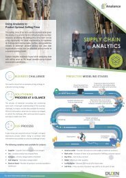
Track, control, and improve drug sales
with Analance
The Pharma and Life Sciences industry is dealing with many
problems, including increased regulatory oversight, decreased
R&D productivity, challenges to growth and profitability, and the
impact of digitization in the value chain. On top of increasing
costs for regulatory compliance, the industry is also facing
rising R & D costs, changing customer demographics and
deteriorating health outcomes. The Pharma and Life Sciences
industry can use analytics to improve product pricing, sales
prediction and optimization, regulatory compliance reporting,
drug size and shape optimization, and more.
Sales data forms the most traditional source for data analysis
and analytics, with a history of contributing insights and the
know-hows from marketing, sales, advertising, and other
teams. Modern analytics opens the door to predict trends
through more complex analysis and modeling. Data of various
sizes and shapes can be analyzed to derive actionable insights
and evidence based business recommendations.
PHARMACEUTICAL
AND LIFE SCIENCES
USE CASE
Explore the insights Analance found for a Pharma company
that was looking to tract, control, and eventually improve sales.
BUSINESS CHALLENGE
AND GOAL
Understanding sales data to forecasting sales. However,
missing data created a major challenge for analysis and
trend reporting.
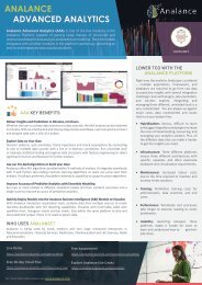
PREDICTIVE MODELING STAGES
Acquiring data from
the data warehouse
Exporatory data and analysis
to check for interralationships
between variables and outcomes
SOLUTIONING
PROCESS AT A GLANCE
Variable selection and
feature engineering
Exporatory data and analysis
to check for interralationships
between variables and outcomes
Data cleansing
The process of statistical consulting and solutioning
starts with a thorough understanding of the business
challenge, its impact, and the data available for analysis.
With this information, we arrive at a solution to mitigate
or control the challenge, offer continued client support,
and adjust models over time.
Modeling
Model validation
and accuracy checking
OUR PROCESS
A data dump was acquired and put through a stringent
exploratory process before trying to correlate what
information was available to solve the challenge at hand.
Deployment
Comparison
of models
ABOUT DUCEN
Ducen IT helps Business and IT users of Fortune 1000 companies with advanced analytics, business intelligence and
data management through its unique end-to-end data science platform called Analance. Analance is an enterpriseclass,
state of the art integrated platform that delivers power and ease of use to business users and data scientists
with a seamless experience and platform scalability to support business growth and strategy.
For more information please visit www.analance.com

THE MODELING PROCESS:
AN INTRODUCTION TO TIME SERIES
TIME SERIES MODELING FLOW CHART
A time series model is the process of modeling serial data to find trends within
and/or across the data under consideration. Every time series is composed of three
components:
• Trend-cycle component.
• Seasonal effects.
• Irregular fluctuation or error.
The main assumption of time series is that data is stationary. However, techniques
also exist to handle data that is not stationary.
How do we check to see if the time series is stationary or not?
To understand if the time series is stationary or not, we used the kpss (Kwiatkowski–
Phillips–Schmidt–Shin), pp (Phillips-Perron), and ADF (AdjustedDickey-Fuller) tests.
The tests assume that the null hypothesis of the series is stationary. A null hypothesis
is a hypothesis of no predictability in the data. Subsequently, from the test results,
if the lag parameter is 3 or less, the stationarity assumption can be accepted, and, if
the p value is less than 0.05, the stationarity assumption can be rejected.
Seasonal effects:
A seasonal effect is a systematic and calendar related effect. Some examples include
the sharp escalation in most Retail series which occurs around December in response
to the Christmas period, or an increase in water consumption in summer due to
warmer weather. An example can be seen below.
Figure 2: Seasonal component visualized.
THERE ARE TWO TYPES OF SEASONALITIES:
AND ADDITIVE AND MULTIPLICATIVE
Assuming a time series with changes in the level, the seasonal component may
interact with the level in an additive or multiplicative way. This essentially means
that in the first case the amplitude of the seasonality remains constant, while in the
latter it changes as the level does. Figure 3 provides an example of an additively and
a multiplicatively seasonal time series.
If the level is decreasing, under multiplicative seasonality the seasonal amplitude
would get smaller while in the case of additive seasonality it would remain constant.
For more information please visit www.analance.com

Figure 3. Additively and multiplicatively seasonal time series.
When to apply an additive decomposition?
The behaviors of the components are independent from each other. For instance, an
increase in the trend-cycle will not cause an increase in the magnitude of seasonal
dips and troughs. The difference of the trend and the raw data is roughly constant
in similar periods of time (months, quarters, etc.) irrespective of the tendency of
the trend. The pattern of seasonal variation is roughly stable over the year, i.e., the
seasonal movements are approximately the same from year to year.
When to apply a multiplicative decomposition?
The multiplicative model is particularly appropriate if the seasonal and irregular
fluctuations change in a specific manner, as a result of trend behavior. In this type
of relationship, the amplitude of the seasonality increases (or decreases) with
an increasing (or decreasing) trend, therefore, contrary to the additive case, the
components are not independent from each other.
Trends
A trend is a long-term direction component of a series and is seen to either be
increasing, or decreasing on a consistent basis along time. An example can be seen
below.
ABOUT DUCEN
Figure 4. Trend component visualized.
If there are multiple trends and seasonality factors, the data needs to be detrended
and de-seasonalized multiple times. For data where trends and seasonality
continuously persist even after de-trending or de-seasonalizing, appropriate models
that accommodate trends and seasonalities are chosen for the analysis. Once the
appropriate models are chosen based on the flow chart above, the analysis can
either end or be reiterated.
A point to note is that when the forecast residuals are correlated, and/or when
there are no stark patterns or additivity seen, i.e., the data already looks stable, it is
wise to take the ARIMA modeling approach.
Ducen IT helps Business and IT users of Fortune 1000
companies with advanced analytics, business intelligence
and data management through its unique end-to-end data
science platform called Analance. Analance is an enterpriseclass,
state of the art integrated platform that delivers power
and ease of use to business users and data scientists with
a seamless experience and platform scalability to support
business growth and strategy.
Apart from the most commonly used decomposition schemes, there are other
models describing the relationship between components. One of the most popular
ones is pseudo-additive decomposition.
For more information please visit www.analance.com

Pseudo – additive model:
This model combines some features of both the additive and the multiplicative
models. The conclusion that follows is that the pseudo-additive model assumes
that seasonal and irregular components are both dependent on the trend behavior,
and at the same time, are independent from each other. This model has been designed
for those time series that fundamentally display multiplicative relationships
between components, yet the time series may have values equal or close to zero, in
which case the multiplicative decomposition cannot be applied. The pseudo-additive
model allows allocation of zero values either to the seasonal or to the irregular
components, leaving the trend-cycle unaffected by it. After finding the right model,
the residuals are checked for correlation, and, normality with mean (arithmetic average)
0, and constancy in variance by using a histogram of the residuals, passing
which the model can be deployed to forecast real values.
After this, the following models can be considered: ARIMA(p,d), ARI-
MA(d,q), or ARIMA(p,d,q). After finding the right model, the residuals are
checked for auto correlation using the Ljung-Box test with no autocorrelation
as the null hypothesis, passing which, for normality with mean
(Arithmetic average) 0 and constancy in variance by using a histogram
of the residuals, passing which the model can be deployed to forecast
real values, failing which indicates the need for other more complex time
series models be considered.
FINDINGS AND ANALYSIS
Failing the no correlation requirement, the modeling scene switches to the ARIMA
family.
ARIMA models:
ARIMA models: ARIMA stands for Auto Regressive Integrated Moving Average. For
fitting ARIMA models, it is important for the series to be stationary. If the series is
not stationary, then the series needs to be differenced. The number of times the
series is differenced contributes to the ‘d’ parameter in ARIMA(p, d), ARIMA(d, q),
and ARIMA(p, d, q). Following this, the differenced series is analyzed by constructing
a correlogram which looks for auto-correlation. The auto correlation function finds
the parameter p if the pth serial value exceeds the confidence bands seen below.
• Analysis looked at 147 products sold over a period of 69 months.
• Complete yearly data was available for 35 (24%) products.
• Sales peaked in April for every product.
• First and third quarter showed low sales every year and contributed
to 6 months of lull.
• Low sales influenced by regulatory changes were assigned a moving
average.
The data was segmented and analyzed based on location of each ATM.
The above-mentioned findings, along with the seasonal patterns observed
(strong weekly seasonality) in the dataset of each ATM, enabled
us to choose the appropriate algorithm (Holt Winters with seasonal adjustments).
The industry standard MAPE (Mean Absolute Percentage Error) was
used to estimate the prediction error. A range of 50 – 60% was achieved
from the data under consideration.
CONCLUSION
Figure 5: The auto correlation / correlogram plot.
Similarly, the partial auto correlation function finds the parameter q if the qth serial
value exceeds the confidence bands as seen below.
Having a model such as the one developed above can enable banks
to replenish ATMs more efficiently and reduce cash redundancy in
machines. The cash saved in this manner can be mobilized to offer
loans and other financial services, resulting in profit/income for the
banks.
Time series has been found to be most effective in areas such as business
or economic forecasting of events across time. A set of models
has been very successful in predicting outcomes when little or no
information is known about related background processes and/or
features affecting the outcome. Model forecasting accuracy can be
increased by adopting the regression approach if there is good quality
data available, such as day of the week of withdrawal, week of the
month, month of the year, dates of relevant events such as festivals
or sporting events.
Figure 6: The partial auto – correlation / partial correlogram plot.
For more information please visit www.analance.com