Sensitivity analysis of crop growth simulation model performance to crop and weather input data
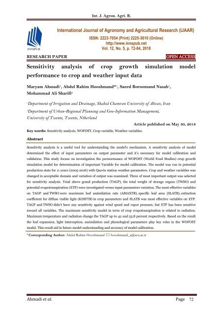
Sensitivity analysis is a useful tool for understanding the model's mechanism. A sensitivity analysis of model determined the effect of input parameters on output parameter and it’s necessary for model calibration and validation. This study focuse on investigation the permormance of WOFOST (World Food Studies) crop growth simulation model for determination of important Variable for model calibration. The model was run in potential production state for 11 years (2005-2016) with Qazvin station weather parameters. Crop and weather variables was changed in acceptable domain and variation of output was examined. Three of most important output was selected for sensitivity analysis. Total above grand production (TAGP), the total weight of storage organs (TWSO) and potential evapotranspiration (ETP) were investigated versus input parameters variation. The most effective variables on TAGP and TWSO were maximum leaf assimilation rate (AMAXTB), specific leaf area (SLATB), extinction coefficient for diffuse visible light (KDIFTB) in crop parameters and SLATB was most effective variables on ETP. TAGP and TWSO didn’t have any sensitivity against wind speed and vapor pressure, but ETP has been sensitive toward all variables. The maximum sensitivity model in term of crop evapotranspiration is related to radiation. Maximum temperature and radiation change the TAGP up to 42 and 55.8 percent respectively. Based on the result the leaf expansion, light interception, assimilation and phenological parameters play key roles in the WOFOST model. This result aid in future model understanding and accuracy of model calibration.
Sensitivity analysis is a useful tool for understanding the model's mechanism. A sensitivity analysis of model determined the effect of input parameters on output parameter and it’s necessary for model calibration and validation. This study focuse on investigation the permormance of WOFOST (World Food Studies) crop growth simulation model for determination of important Variable for model calibration. The model was run in potential production state for 11 years (2005-2016) with Qazvin station weather parameters. Crop and weather variables was changed in acceptable domain and variation of output was examined. Three of most important output was selected for sensitivity analysis. Total above grand production (TAGP), the total weight of storage organs (TWSO) and potential evapotranspiration (ETP) were investigated versus input parameters variation. The most effective variables on TAGP and TWSO were maximum leaf assimilation rate (AMAXTB), specific leaf area (SLATB), extinction
coefficient for diffuse visible light (KDIFTB) in crop parameters and SLATB was most effective variables on ETP. TAGP and TWSO didn’t have any sensitivity against wind speed and vapor pressure, but ETP has been sensitive toward all variables. The maximum sensitivity model in term of crop evapotranspiration is related to radiation.
Maximum temperature and radiation change the TAGP up to 42 and 55.8 percent respectively. Based on the result the leaf expansion, light interception, assimilation and phenological parameters play key roles in the WOFOST model. This result aid in future model understanding and accuracy of model calibration.

You also want an ePaper? Increase the reach of your titles
YUMPU automatically turns print PDFs into web optimized ePapers that Google loves.
Int. J. Agron. Agri. R.<br />
International Journal <strong>of</strong> Agronomy <strong>and</strong> Agricultural Research (IJAAR)<br />
ISSN: 2223-7054 (Print) 2225-3610 (Online)<br />
http://www.innspub.net<br />
Vol. 12, No. 5, p. 72-84, 2018<br />
RESEARCH PAPER<br />
OPEN ACCESS<br />
<strong>Sensitivity</strong> <strong>analysis</strong> <strong>of</strong> <strong>crop</strong> <strong>growth</strong> <strong>simulation</strong> <strong>model</strong><br />
<strong>performance</strong> <strong>to</strong> <strong>crop</strong> <strong>and</strong> <strong>weather</strong> <strong>input</strong> <strong>data</strong><br />
Maryam Ahmadi 1 , Abdul Rahim Hooshm<strong>and</strong>* 1 , Saeed Boroom<strong>and</strong> Nasab 1 ,<br />
Mohammad Ali Sharifi 2<br />
1<br />
Department <strong>of</strong> Irrigation <strong>and</strong> Drainage, Shahid Chamran University <strong>of</strong> Ahvaz, Iran<br />
2<br />
Department <strong>of</strong> Urban-Regional Planning <strong>and</strong> Geo-Information Management,<br />
University <strong>of</strong> Twente, Twente, Ntherl<strong>and</strong><br />
Article published on May 30, 2018<br />
Key words: <strong>Sensitivity</strong> <strong>analysis</strong>, WOFOST, Crop variable, Weather variables.<br />
Abstract<br />
<strong>Sensitivity</strong> <strong>analysis</strong> is a useful <strong>to</strong>ol for underst<strong>and</strong>ing the <strong>model</strong>'s mechanism. A sensitivity <strong>analysis</strong> <strong>of</strong> <strong>model</strong><br />
determined the effect <strong>of</strong> <strong>input</strong> parameters on output parameter <strong>and</strong> it’s necessary for <strong>model</strong> calibration <strong>and</strong><br />
validation. This study focuse on investigation the permormance <strong>of</strong> WOFOST (World Food Studies) <strong>crop</strong> <strong>growth</strong><br />
<strong>simulation</strong> <strong>model</strong> for determination <strong>of</strong> important Variable for <strong>model</strong> calibration. The <strong>model</strong> was run in potential<br />
production state for 11 years (2005-2016) with Qazvin station <strong>weather</strong> parameters. Crop <strong>and</strong> <strong>weather</strong> variables was<br />
changed in acceptable domain <strong>and</strong> variation <strong>of</strong> output was examined. Three <strong>of</strong> most important output was selected<br />
for sensitivity <strong>analysis</strong>. Total above gr<strong>and</strong> production (TAGP), the <strong>to</strong>tal weight <strong>of</strong> s<strong>to</strong>rage organs (TWSO) <strong>and</strong><br />
potential evapotranspiration (ETP) were investigated versus <strong>input</strong> parameters variation. The most effective variables<br />
on TAGP <strong>and</strong> TWSO were maximum leaf assimilation rate (AMAXTB), specific leaf area (SLATB), extinction<br />
coefficient for diffuse visible light (KDIFTB) in <strong>crop</strong> parameters <strong>and</strong> SLATB was most effective variables on ETP.<br />
TAGP <strong>and</strong> TWSO didn’t have any sensitivity against wind speed <strong>and</strong> vapor pressure, but ETP has been sensitive<br />
<strong>to</strong>ward all variables. The maximum sensitivity <strong>model</strong> in term <strong>of</strong> <strong>crop</strong> evapotranspiration is related <strong>to</strong> radiation.<br />
Maximum temperature <strong>and</strong> radiation change the TAGP up <strong>to</strong> 42 <strong>and</strong> 55.8 percent respectively. Based on the result<br />
the leaf expansion, light interception, assimilation <strong>and</strong> phenological parameters play key roles in the WOFOST<br />
<strong>model</strong>. This result aid in future <strong>model</strong> underst<strong>and</strong>ing <strong>and</strong> accuracy <strong>of</strong> <strong>model</strong> calibration.<br />
* Corresponding Author: Abdul Rahim Hooshm<strong>and</strong> hooshm<strong>and</strong>_a@scu.ac.ir<br />
Ahmadi et al. Page 72
Int. J. Agron. Agri. R.<br />
Introduction<br />
Calibration is a dem<strong>and</strong>ing <strong>and</strong> critical step for using<br />
<strong>crop</strong> <strong>growth</strong> <strong>simulation</strong> <strong>model</strong>s (Gilardelli et al.,<br />
2018). It has been shown that application <strong>of</strong> a <strong>crop</strong><br />
<strong>growth</strong> <strong>simulation</strong> <strong>model</strong> outside the domain for<br />
which it was developed <strong>and</strong> calibrated for, <strong>of</strong>ten leads<br />
<strong>to</strong> disappointing results (Kabat et al., 1995). Before<br />
calibration underst<strong>and</strong>ing the <strong>model</strong> behavior versus<br />
each <strong>input</strong> variables is necessary. <strong>Sensitivity</strong> <strong>analysis</strong><br />
is a helpful method for increasing the knowledge<br />
about <strong>model</strong> <strong>performance</strong>. WOFOST <strong>model</strong> is used in<br />
several research domain such as climate change<br />
(Gilardelli et al., 2018), yield forecasting (Ma et al.,<br />
2013), yield gap (Boogaard et al., 2013) water stress<br />
(Kroes <strong>and</strong> Supit, 2011) <strong>and</strong> <strong>data</strong> assimilation (de Wit<br />
et al., 2012; Gilardelli et al., 2018; Huang et al., 2015;<br />
Ma et al., 2013). Therefore choosing the appropriated<br />
variables for calibration <strong>and</strong> measurement in the field<br />
is important for using <strong>of</strong> WOFOST applying.<br />
<strong>Sensitivity</strong> <strong>analysis</strong> “SA” is a procedure <strong>to</strong> determine<br />
the effect <strong>of</strong> different value <strong>of</strong> <strong>input</strong> parameters on<br />
output parameters. <strong>Sensitivity</strong> <strong>analysis</strong> is used <strong>to</strong> find<br />
important <strong>and</strong> most effective variables on any <strong>model</strong><br />
outputs. There are basically two general methods for<br />
sensitivity <strong>analysis</strong>, local <strong>and</strong> global methods. In the<br />
local methods, one <strong>input</strong> is varied <strong>and</strong> other <strong>input</strong>s<br />
are kept fixed as default value. This method is used in<br />
several types <strong>of</strong> research because it is a quick <strong>and</strong> easy<br />
<strong>to</strong> use (Wang et al., 2013). Another method is global<br />
sensitively <strong>analysis</strong>, which in this method the entire<br />
range <strong>of</strong> <strong>input</strong>s are considered. There are many<br />
algorithms for global SA such as screening methods,<br />
regression-based methods, <strong>and</strong> variance-based<br />
methods (Confalonieri et al., 2012).<br />
Screening methods is based on calculation <strong>of</strong><br />
elementary effects <strong>of</strong> each fac<strong>to</strong>r as well as their<br />
average, then estimating the <strong>to</strong>tal fac<strong>to</strong>r importance<br />
on the <strong>model</strong> outputs that are known as the Morris<br />
method(Campolongo et al., 2007). Richtera et al<br />
(2010) used Morris method <strong>to</strong> yield formation <strong>of</strong><br />
Durum wheat <strong>and</strong> prove that Morris is a reliable <strong>and</strong><br />
effective method for determining effective <strong>and</strong><br />
important parameters for <strong>model</strong> optimizing (Richtera<br />
et al., 2010b).<br />
Confalonieri et al. 2010 used Morris <strong>and</strong> Sobol<br />
sensitivity <strong>analysis</strong> methods for the rice <strong>model</strong><br />
WARM in Europe in deferent climate <strong>and</strong> locations<br />
(Confalonieri et al., 2010). Regression-based methods<br />
such as Latin Hypercube Sampling (LHS) R<strong>and</strong>om<br />
<strong>and</strong> Quasi-R<strong>and</strong>om LpTau is based on the<br />
computation <strong>of</strong> st<strong>and</strong>ard or partial regression<br />
coefficients. this method is assessing the effect <strong>of</strong><br />
changing variables (Confalonieri et al., 2012).<br />
Variance-based methods is used for computation <strong>of</strong><br />
the variance <strong>of</strong> the output(s) in<strong>to</strong> terms<br />
corresponding <strong>to</strong> the different <strong>input</strong>s <strong>and</strong> their<br />
interactions (Marzban, 2013).<br />
<strong>Sensitivity</strong> is a technique exploring <strong>model</strong> uncertainty<br />
as well as identifying the contribution <strong>of</strong> each<br />
parameter <strong>to</strong> the <strong>model</strong> response (Oakley <strong>and</strong><br />
O'Hagan, 2004; Richtera et al., 2010a).<br />
Confalonieri et al. (2006) have assessed the<br />
sensitivity <strong>analysis</strong> <strong>of</strong> WOFOST for rice biomass<br />
<strong>simulation</strong>s. Based on this research final biomass<br />
showed high variability <strong>to</strong>ward the <strong>input</strong>s especially<br />
CO2 assimilation rates <strong>and</strong> partitioning coefficients<br />
was the most relevant.(Confalonieri et al., 2006b).<br />
Wang <strong>and</strong> et al used Fourier Amplitude <strong>Sensitivity</strong><br />
Test method for WOFOST sensitivity <strong>analysis</strong> <strong>and</strong><br />
show that some parameters don’t have a direct effect<br />
on biomass but play a key role in certain stage<br />
through the plant <strong>growth</strong>. Farhadi <strong>and</strong> et al. (2009)<br />
survey the sensitivity <strong>of</strong> WOFOST <strong>model</strong> <strong>to</strong> daily solar<br />
radiation estimation methods <strong>and</strong> their result show<br />
that sensitivity <strong>analysis</strong> is necessary for <strong>model</strong> use<br />
<strong>and</strong> maximum deviation for winter barley <strong>and</strong> silage<br />
maize was 9% variability (Bansouleh et al., 2009)<br />
Kanellopoulos et al. (2014) used the WOFOST <strong>model</strong><br />
for climate change assessment in socio economic<br />
scenario for assessment the impact <strong>of</strong> climate change<br />
<strong>and</strong> socio-economic scenarios on arable farming<br />
system (Kanellopoulos et al., 2014).<br />
<strong>Sensitivity</strong> <strong>analysis</strong> can be helpful for improvement <strong>of</strong><br />
<strong>model</strong> calibration <strong>and</strong> can be used as a guide for use<br />
<strong>of</strong> <strong>model</strong>. The aim <strong>of</strong> this research is <strong>to</strong> investigate the<br />
WOFOST <strong>model</strong> <strong>performance</strong> <strong>to</strong>ward <strong>weather</strong> <strong>and</strong><br />
<strong>crop</strong> variable variation <strong>of</strong> Qazvin plean.<br />
Ahmadi et al. Page 73
Int. J. Agron. Agri. R.<br />
Materials <strong>and</strong> methods<br />
Model<br />
The WOFOST <strong>model</strong> is a <strong>to</strong>ol for assessing the <strong>crop</strong><br />
<strong>growth</strong> <strong>and</strong> production under a wide range <strong>of</strong> <strong>weather</strong><br />
<strong>and</strong> soil conditions. WOFOST <strong>model</strong> is used not only<br />
for <strong>crop</strong> production limitations such as light, moisture<br />
<strong>and</strong> macro-nutrients but also for estimate what<br />
improvement is possible. The WOFOST use plant<br />
physiology <strong>and</strong> environmental variables <strong>to</strong> <strong>simulation</strong><br />
plant <strong>growth</strong> <strong>and</strong> calculation yield <strong>and</strong> dry<br />
matter production in potential <strong>and</strong> water <strong>and</strong> nutrient<br />
limitation (van Diepen et al., 1989) Simulation <strong>of</strong><br />
<strong>crop</strong> <strong>growth</strong> in WOFOST <strong>model</strong> is done based on<br />
<strong>weather</strong> parameters (temperature, sunshine, vapor<br />
pressure, wind speed, <strong>and</strong> rain) soil properties<br />
(moisture in field capacity (FC), wilting point (WP),<br />
hydraulic conductivity in saturation (k0) <strong>and</strong> soil<br />
depth) <strong>and</strong> <strong>crop</strong> physiological <strong>and</strong> phenological<br />
properties (Boogaard et al., 2014). WOFOST <strong>model</strong> is<br />
used in CGMS1 for moni<strong>to</strong>ring <strong>growth</strong> in regional <strong>and</strong><br />
nationals scale. Model is linked <strong>to</strong> geographic system<br />
<strong>and</strong> related <strong>data</strong>base for yield forecasting <strong>and</strong> <strong>crop</strong><br />
state moni<strong>to</strong>ring in several studies (Boogaardb et al.,<br />
2013; KODEŠOVÁ1 <strong>and</strong> BRODSKÝ2, 2006; LAZAR et<br />
al., 2009).<br />
WOFOST is a dynamic <strong>model</strong> for <strong>simulation</strong> <strong>crop</strong><br />
<strong>growth</strong> in daily rate <strong>and</strong> in three conditions, a<br />
Potential production that <strong>crop</strong> <strong>growth</strong> may be limited<br />
by light <strong>and</strong> temperature regime only. In this<br />
condition, water <strong>and</strong> nutrient supply are taken <strong>to</strong> be<br />
optimum. In water, limited production water supply<br />
may be limited in <strong>crop</strong> <strong>growth</strong> period while nutrient<br />
supply is taken <strong>to</strong> be optimum. The last <strong>model</strong> state is<br />
Nutrient limited production, in this <strong>model</strong> state in<br />
addition <strong>to</strong> water limitation, soil nutrient supply is<br />
also considered limiting fac<strong>to</strong>r for production<br />
(Ittersum <strong>and</strong> Rabbinge, 1997). In this research,<br />
based on literature survey (Bahman, 2009; Bansouleh<br />
et al., 2009; Confalonieri et al., 2006b; Vazifedoust,<br />
2007) some <strong>of</strong> the more important parameters (<strong>crop</strong>,<br />
<strong>and</strong> <strong>weather</strong>) were chosen for sensitivity <strong>analysis</strong><br />
(Table 1 <strong>and</strong> 2). Crop <strong>and</strong> <strong>weather</strong> variables: Table 1<br />
<strong>and</strong> Table 2 Present the selected <strong>crop</strong>, <strong>weather</strong><br />
variables for investigation the <strong>model</strong> behavior <strong>to</strong>ward<br />
the increasing <strong>and</strong> decreasing trend <strong>of</strong> these<br />
variables. The WOFOST <strong>model</strong> was calibrated based<br />
<strong>of</strong> phonological date <strong>of</strong> field study <strong>and</strong> temperature<br />
sum from emergence <strong>to</strong> flowering (TSUM1) <strong>and</strong> for<br />
flowering <strong>to</strong> maturity (TSUM2) for barley which was<br />
calculated receptivity 780,800.<br />
Table 1. Crop parameters for sensitivity <strong>analysis</strong>.<br />
Parameter Unit Rang Default Value Description<br />
SLATB Ha/kg<br />
0.00070-<br />
0.00420<br />
KDIFTB - 0.44- 1.0<br />
EFFTB kg /(ha hr) 0.4-0.5<br />
AMAXTB kg/(ha.hr) 1-70<br />
0 0.3 0.9 1.45 2 Specific leaf area as a function <strong>of</strong><br />
0.002 0.0035 0.0025 0.0022 0.0022 DVS<br />
0 2 extinction coefficient for diffuse<br />
0.44 0.44<br />
visible light as a function <strong>of</strong> DVS<br />
0 40 light-use efficiency, single leaf as<br />
0.4 0.4<br />
function <strong>of</strong> daily mean temp.<br />
0 1.2 2 maximum leaf CO2 assimilation as<br />
35 35 5 function <strong>of</strong> DVS<br />
span days 17-50 25<br />
life span <strong>of</strong> leaves growing at 35<br />
Celsius<br />
TDWI Kg/ha 0.5-300 150 Initial <strong>to</strong>tal <strong>crop</strong> dry weight<br />
CFET - 0.8-1.2 1.19<br />
Correction fac<strong>to</strong>r for<br />
evapotranspiration in relation <strong>to</strong> the<br />
reference <strong>crop</strong><br />
RGRLAI Ha/(ha.d) 0.007-0.5 0.0075 Maximum relative increase in LAI<br />
TSUM1 ºC/d 150-1050 1123<br />
Thermal time from emergence <strong>to</strong><br />
anthesis<br />
TSUM2 ºC/d 600-1550 893<br />
Thermal time from anthesis <strong>to</strong><br />
maturity<br />
Ahmadi et al. Page 74
Int. J. Agron. Agri. R.<br />
Table 2. Weather parameters for sensitivity <strong>analysis</strong>.<br />
Parameter Unit Default value<br />
minimum temperature °c Weather station reports<br />
maximum temperature °c Weather station reports<br />
vapor pressure KPa Weather station reports<br />
mean wind speed m/ s Weather station reports<br />
precipitation Mm/ d Weather station reports<br />
irradiation kJ /(m d) Weather station reports<br />
Stady area<br />
The study area is Qazvin plain that located in the<br />
north-west <strong>of</strong> Iran (Fig. 1). QAZVIN station is located<br />
in 36 15N <strong>and</strong> 50 3E <strong>and</strong> in 1279.2 meter elevation<br />
from the sea surface.<br />
Mean annual precipitation <strong>and</strong> average <strong>of</strong> minimum<br />
<strong>and</strong> maximum temperature during the years 1987<br />
until 2003, was 210mm, 2 <strong>and</strong> 18°C, respectively. In<br />
this study daily <strong>weather</strong> parameters <strong>of</strong> Qazvin station<br />
were used (2000-2011).<br />
Fig. 1. The study area (The location <strong>of</strong> Qazvin province <strong>and</strong> Qazvin plain in Iran).<br />
<strong>Sensitivity</strong> <strong>analysis</strong><br />
<strong>Sensitivity</strong> <strong>analysis</strong> was done based on the variation<br />
<strong>of</strong> one variable in time. Variation was done based on<br />
the acceptable domain <strong>of</strong> each variable for the <strong>model</strong>.<br />
The <strong>model</strong> was run for winter barley with Qazvin<br />
daily <strong>weather</strong> parameters. For investigating the<br />
impact <strong>of</strong> variables changing <strong>to</strong> outputs The WOFOST<br />
<strong>model</strong> was run in increasing <strong>and</strong> decreasing trend <strong>of</strong><br />
variables. In increasing Trent The variables were<br />
changed between +10% <strong>to</strong> +50% with 10% steps <strong>and</strong><br />
in decreasing trend changing was done between -10%<br />
<strong>to</strong> -50% with -10% steps. The trend has been s<strong>to</strong>pped<br />
upon some variables got out <strong>of</strong> range <strong>of</strong> acceptablity.<br />
There are some exception because 10% cause <strong>to</strong> high<br />
values for some variables. TSUM1 <strong>and</strong> TSUM 2 was<br />
change in -10% <strong>to</strong> +10% domain with 2% steps <strong>and</strong><br />
for CEFT between +10% <strong>to</strong> -10% with 5% steps.<br />
Total above ground production (TAGP), the <strong>to</strong>tal<br />
weight <strong>of</strong> s<strong>to</strong>rage organ (TWSO) <strong>and</strong> potential<br />
evapotranspiration (ETP) was selected for moni<strong>to</strong>ring<br />
the variation in output parameters.<br />
<strong>Sensitivity</strong> index (SI)<br />
The equation for sensitivity index is Absolute<br />
<strong>Sensitivity</strong>. This question is for linearized sensitivity<br />
equation, can be used "rate <strong>of</strong> change in one fac<strong>to</strong>r<br />
with respect <strong>to</strong> change in another fac<strong>to</strong>r" that can<br />
show the linearized sensitivity.<br />
SI = (O 2 − O 1 )<br />
(I 2 − I 1 )<br />
Where O 2 − O 1 is the change in <strong>model</strong> output for a<br />
change in <strong>model</strong> <strong>input</strong> I 2 − I 1 .(QUINTON, 1994).<br />
<strong>Sensitivity</strong> index was calculated for Biomass, <strong>crop</strong> yield<br />
<strong>and</strong> evapotranspiration versus such <strong>input</strong> variables.<br />
Ahmadi et al. Page 75
Int. J. Agron. Agri. R.<br />
Results<br />
Crop variables<br />
<strong>Sensitivity</strong> <strong>analysis</strong> <strong>of</strong> <strong>crop</strong> variables measured by<br />
TAGP shows the result <strong>of</strong> sensitivity <strong>analysis</strong> for <strong>crop</strong><br />
variables measured by TAGP. Table 3, present the<br />
sensitivity index (SI) <strong>of</strong> TAGP, TWSO <strong>and</strong> ETP<br />
against <strong>crop</strong> variables variation.<br />
Model has different behavior with variables variation.<br />
SLATB, KDIFTB <strong>and</strong> AMAXTB have most effective<br />
parameters on TAGP variation. TAGP values are<br />
between 1800-2300 kg/ha including any outliers but<br />
actual maximum <strong>and</strong> minimum are 7500 <strong>and</strong><br />
23000kg/ha respectively (Fig. 3). Outliers are the<br />
result <strong>of</strong> -50% SLATB variations that is more than<br />
±1.5 interquartile range. The distribution is skewed<br />
left because most <strong>of</strong> the observations are<br />
concentrated on the low end <strong>of</strong> the scale. All TAGP<br />
values are less than normal run (without any<br />
variation in output) but in positive variation (+10 <strong>to</strong><br />
+40%) TAGP variation has an upward tendency with<br />
low slope but in negative variation (-10% <strong>to</strong> -50%)<br />
present a downward tendency but with a slop higher<br />
than upward (Fig. 2.A). SI for SLATB is 1.03 that<br />
confirms the <strong>model</strong> sensitivity <strong>to</strong> this variable.<br />
Table 3. <strong>Sensitivity</strong> <strong>analysis</strong> index (SI) <strong>of</strong> output for <strong>crop</strong> variables.<br />
Variables TAGP TWSO ETP<br />
SLATB 0.55 0.43 0.44<br />
KDIFTB 0.70 0.56 0.21<br />
SPAN 1 0.51 0.41<br />
TDWI 0.79 0.01 0.09<br />
EFFTB 0.72 0.67 0.14<br />
RGRLAI 0.05 6.58 0.09<br />
AMAXTB 0.75 0.13 0.75<br />
TSUM1 0.59 0.78 0.83<br />
TSUM2 0.32 0.48 0.22<br />
Fig. 2. TAGP variation versus variation <strong>of</strong> <strong>crop</strong> parameters (%).<br />
Fig. 3. Distribution <strong>of</strong> TAGP versus <strong>crop</strong> variable variation.<br />
Ahmadi et al. Page 76
Int. J. Agron. Agri. R.<br />
KDIFTB has changed TAGP with right skewed with<br />
0.7 for sensitivity index (SI) (Fig.3). Model is more<br />
sensitive against <strong>to</strong> decreasing the KDIFTB values<br />
because the slope <strong>of</strong> increasing trend higher than<br />
decreasing trend (Fig. 2.B).<br />
TAGP has same behavior <strong>to</strong>ward variation <strong>of</strong> SPAN<br />
but with SI=1 (Table 3 <strong>and</strong> Fig. 2). TAGP has a<br />
normal distribution with TDWI variation (The middle<br />
half <strong>of</strong> a <strong>data</strong> set falls within the interquartile range).<br />
One <strong>of</strong> the <strong>data</strong> was considered as the outlier that is<br />
output in 2012-2013 without any variation in <strong>input</strong>.<br />
SI was achieved 0.79 for this parameter <strong>and</strong> it is<br />
shown moderate <strong>model</strong> sensitivity versus TDWI.<br />
Distribution <strong>of</strong> TAGP within EFFTB variation is<br />
approximately same as TDWI but with higher values<br />
<strong>and</strong> left skewed (Fig.2). TAGP has right skewed with<br />
RGRLAI variation (Fig. 2.E) .The <strong>model</strong> SI was<br />
achieved 0.05 that present the low <strong>model</strong> sensitivity<br />
versus these variables.<br />
The highest variation for TAGP is occurred with<br />
AMAXTB variation with 0.76 for SI. TAGP variation<br />
is between 8200-28700 kg/ha with a little right<br />
skewed. TAGP has increasing trend with positive<br />
variation <strong>and</strong> vice versa for negative variation. Model<br />
behavior against TSUM1 <strong>and</strong> TSUM2 is different<br />
although median (<strong>of</strong> the cross line in the middle) is<br />
same for this variation. TAGP variations have right<br />
skewed while TSUM2 has normal distribution. Model<br />
SI for these variables was achieved 0.62 <strong>and</strong> .32 for<br />
TSUM1 <strong>and</strong> TSUM2 respectively.<br />
<strong>Sensitivity</strong> <strong>analysis</strong> <strong>of</strong> <strong>crop</strong> variables measured by<br />
TWSO:<br />
Fig. 4 shows the behavior <strong>of</strong> <strong>to</strong>tal weight <strong>of</strong> s<strong>to</strong>rage<br />
organ vesus <strong>crop</strong> variable variation <strong>and</strong> Fig. 5<br />
represents the wariation <strong>of</strong> this parameter <strong>to</strong>ward<br />
variable variation. TWSO is more sensitive against <strong>to</strong><br />
decreasing the KDIFTB values because the slope <strong>of</strong><br />
increasing trend higher than decreasing trend.<br />
Distribution <strong>of</strong> TWSO values is normal with 0.44<br />
value for SI. Maximum variation for increasing<br />
SLATB is 6% while for negative variation is 58% <strong>of</strong><br />
default value.<br />
TWSO sensitivity is moderate (SI=0.56) <strong>and</strong> with<br />
right skewed distribution versus variation <strong>of</strong> KDIFTB<br />
(Table 4 <strong>and</strong> Fig. 4). Maximum vaiation in TWSO is<br />
42% with half <strong>of</strong> default value for EFFTB. SNAP<br />
variation has made a normal distribution <strong>of</strong> TWSO<br />
with 0.51 for sensitivity index. While Maximum<br />
variation was achieved 24% for -50% variation in the<br />
span (Fig. 4.C).<br />
Model has very low <strong>Sensitivity</strong> <strong>to</strong>ward RGRLAI <strong>and</strong><br />
TWSO variations with SI= 0.02 <strong>and</strong> 0.07 respectivity.<br />
TWSO distribution with variation in AMAXTB has the<br />
high value compare with other variables with normal<br />
distribution. Model sensitivity for decreasing pattern<br />
is more than increasing pattern <strong>of</strong> AMAXTB. SI value<br />
for these variables is 0.75 that shows the high<br />
sensitivity <strong>of</strong> TWSO <strong>to</strong>ward AMAXTB variables.<br />
TWSO shows approximately same behavior with TSUM1<br />
<strong>and</strong> TSUM2 variation but outlets for TSUM1 is for 2012-<br />
2013 but for TSUM2 2010-2011. TWSO has normal <strong>and</strong><br />
left skewed distribution for TSUM1 <strong>and</strong> TSUM2<br />
variations.SI is 0.48 <strong>and</strong> 0.79 for TSUM1 <strong>and</strong> TSUM2<br />
respectively that shows TWSO is more sensitivity <strong>to</strong>ward<br />
TSUM2. Fig 4.H <strong>and</strong> Fig 4. I confirm this because<br />
maximum variation with TSUM1 variation is 10% while<br />
for TSUM2 is around 6 percent.<br />
<strong>Sensitivity</strong> <strong>analysis</strong> <strong>of</strong> <strong>crop</strong> variables measured by<br />
ETP<br />
Fig.6 <strong>and</strong> Fig.7 show the behavior <strong>of</strong> ETP against <strong>crop</strong><br />
variables variation. Based on the results SLATB cause<br />
the highest variation <strong>of</strong> ETP. ETP has varied between<br />
211-510mm with left skewed <strong>and</strong> 0.44 value for SI.<br />
Outlets appear when SLATB decreased until 50% <strong>of</strong><br />
difult value. ETP sensitivity for reducing the SLATB is<br />
more than increasing (42% for 50% reducing).<br />
Variation has right skewed <strong>and</strong> SI index was<br />
calculated 0.21 for KADIFTB variation <strong>and</strong> same as<br />
previous variables modle sensitivity versus decreasing<br />
trend is more than the inversing trend. One <strong>of</strong><br />
important variable that effected on ETP is SPAN .SI<br />
index for this variable is ached 0.41 .Variation domain<br />
is same as KDIFTB but with more values <strong>and</strong> left<br />
skewed <strong>and</strong> one outlet for -50% in 2010 -2011.<br />
Variation percent is maximum 9% <strong>and</strong> -20% for<br />
increasing trend.<br />
Ahmadi et al. Page 77
Int. J. Agron. Agri. R.<br />
Fig. 4. TWSO variation versus <strong>crop</strong> variation (%).<br />
Fig. 5. Distribution <strong>of</strong> TWSO versus <strong>crop</strong> variable variation.<br />
Ahmadi et al. Page 78
Int. J. Agron. Agri. R.<br />
Fig. 6. ETP variation versus <strong>crop</strong> variation (%).<br />
Fig. 7. Distribution <strong>of</strong> ETP versus <strong>crop</strong> variable variation.<br />
ETP values have left skewed variation against<br />
TDWI <strong>and</strong> EFFTB <strong>and</strong> right skewed RGRLAI<br />
variation. SI index for these variables are 0.09,<br />
0.14 <strong>and</strong> 0.1 that confirmed <strong>model</strong> sensitivity<br />
<strong>to</strong>ward EFFTB values. As it is shown in Fig. 6.D<br />
ETP is varied maximum 3.6 <strong>and</strong> 5.9% for increased<br />
<strong>and</strong> decreasing trend <strong>of</strong> TDWI while EFFTB change<br />
ETP up <strong>to</strong> 2.8% with 25% changing Fig.6.I.<br />
AMAXTB cause a left skewed distribution for ETP<br />
with outlets that are effect <strong>of</strong> -50% variations in<br />
AMAXTB.<br />
SI index <strong>of</strong> ETP values was calculate 0.13 for this<br />
variable <strong>and</strong> maximum present <strong>of</strong> variation are 3<br />
<strong>and</strong> 14 present for increasing <strong>and</strong> decreasing trend<br />
<strong>of</strong> this variable. TSUM1 <strong>and</strong> TSUM2 show a<br />
different effect on ETP values. Both <strong>of</strong> them have<br />
left skewed but different distribution. SI was<br />
achieved 0.83 <strong>and</strong> 0.23 for TSUM1 <strong>and</strong> TSUM. Fig.<br />
6.H <strong>and</strong> Fig. 6.I shows maximum 7.7 <strong>and</strong> 9%<br />
variation in ETP values for increasing <strong>and</strong><br />
decreasing trend. Maximum variation for TSUM 2<br />
is 1.1-1.7% that confirms the low sensitivity <strong>of</strong> ETP<br />
<strong>to</strong>ward TSUM2.<br />
Ahmadi et al. Page 79
Int. J. Agron. Agri. R.<br />
Weather variables<br />
<strong>Sensitivity</strong> <strong>analysis</strong> <strong>of</strong> <strong>weather</strong> variables measured<br />
by TAGP:<br />
In this part the effect <strong>of</strong> <strong>weather</strong> <strong>input</strong> <strong>model</strong> was<br />
investigated on outputs (TAGP, TWSO, <strong>and</strong> ETP).<br />
Variation <strong>of</strong> rainfall was ignored because the <strong>model</strong><br />
was run in the potential situation. Minimum<br />
temperature (Tmin), maximum (Tmax), vapor<br />
pressure, radiation <strong>and</strong> wind speed that Was varied<br />
between 10 <strong>to</strong> 50 percent in increasing trend ( with<br />
10% steps) <strong>and</strong> -10 <strong>to</strong> -50 percent (with -10% steps).<br />
Fig.8 <strong>and</strong> Fig.9 show the impact <strong>of</strong> <strong>input</strong> variables<br />
variation on TAGP. Based on result vapor pressure<br />
<strong>and</strong> wind speed didn’t have any effect on TAGP.<br />
TAGP has a right-skewed distribution <strong>of</strong> Tmin. There<br />
are two outlets <strong>and</strong> one extreme point on the chart.<br />
These values are related <strong>to</strong> 30, 40 <strong>and</strong> 50 percent<br />
increase in Tmin <strong>and</strong> all occur in 2015-2016. The<br />
extreme point represents those values more than<br />
three times the height <strong>of</strong> the boxes. In these cases, the<br />
mean is greater than the median <strong>and</strong> the greater<br />
mean is caused by these outliers. Based on result,<br />
TAGP show decreasing with increasing (maximum<br />
8.7%) Tmin values <strong>and</strong> vice versa for decreasing<br />
values (maximum 5.5%).<br />
TAGP distribution with Tmax variation is high in<br />
comparison with Tmin. Fig.8.B is confirmed the high<br />
sensitivity <strong>of</strong> TAGP <strong>to</strong>ward Tmax values <strong>and</strong> represent a<br />
trend same as Tmin. Distribution <strong>of</strong> TAGP for radiation<br />
variation is between 4800-22500 kg/ha with right<br />
skewed. As it is clear in Fig 8.C <strong>model</strong> sensitivity <strong>to</strong>ward<br />
increasing trend <strong>of</strong> variations (maximum 11.7) is very<br />
lower than decreasing trend (maximum 55.8%)<br />
Fig. 8. TAGP variation versus <strong>weather</strong> variation (%).<br />
Fig. 9. Distribution <strong>of</strong> TAGP versus <strong>weather</strong> variable variation.<br />
<strong>Sensitivity</strong> <strong>analysis</strong> <strong>of</strong> <strong>weather</strong> variables measured<br />
by TWSO:<br />
As it is shown in Fig.11 TWSO behavior is different for<br />
each variable. Tmin variation created a right-skewed<br />
distribution for TWSO. It is decracing maximum 14%<br />
for increasing trend <strong>of</strong> Tmin <strong>and</strong> 18% for decreasing<br />
trend. TWSO variation in the result <strong>of</strong> Tmax variation<br />
has right-skewed distribution. Outlets <strong>and</strong> extreme<br />
are the result <strong>of</strong> 40% increase in Tmax values that<br />
decreasing 44% <strong>of</strong> TWSO (Fig. 10.B) while for<br />
Ahmadi et al. Page 80
Int. J. Agron. Agri. R.<br />
increasing trend the TWSO variation increasing with<br />
a mild slope up <strong>to</strong> 16.5%. Variation <strong>of</strong> TWSO values<br />
has a normal distribution <strong>and</strong> with unlike trend <strong>of</strong><br />
other <strong>weather</strong> parameters because it has increasing<br />
trend for positive variation <strong>and</strong> decreasing trend with<br />
negative variation (Fig. 11).<br />
Fig. 10. TWSO variation versus <strong>weather</strong> variation (%).<br />
Fig. 11. Distribution <strong>of</strong> TWSO versus <strong>weather</strong> variable variation.<br />
<strong>Sensitivity</strong> <strong>analysis</strong> <strong>of</strong> <strong>weather</strong> variables measured<br />
by ETP:<br />
TAGP <strong>and</strong> TWSO didn’t have any sensitivity against<br />
wind speed <strong>and</strong> vapor pressure but ETP has been<br />
sensitive <strong>to</strong>ward all variables. The maximum<br />
sensitivity <strong>model</strong> in term <strong>of</strong> <strong>crop</strong> evapotranspiration<br />
is related <strong>to</strong> radiation. ETP is varied between 212-547<br />
mm with right-skewed. Tmax variation was changing<br />
ETP in increasing trend maximum -24% <strong>and</strong> 17% in<br />
discerning trend.<br />
Tmin causes a left-skewed distribution with maximum-<br />
3.58 <strong>and</strong> 3.38 % variation for increasing <strong>and</strong> decreasing<br />
trend <strong>of</strong> Tmin. ETP distribution is same for wind speed<br />
<strong>and</strong> vapor pressure. Wind speed has direct effect on<br />
ETP. In increasing trend <strong>of</strong> wind speed maximum ETP<br />
variation is 10% while in decreasing trend is -12% (Fig.<br />
12. A).<br />
The percent <strong>of</strong> vapor pressure is -11% <strong>and</strong> 11% for<br />
increasing <strong>and</strong> decreasing trend <strong>of</strong> Vapor pressure<br />
(Fig. 12.C).<br />
Fig. 12. ETP variation versus <strong>weather</strong> variation (%).<br />
Ahmadi et al. Page 81
Int. J. Agron. Agri. R.<br />
Fig. 13. Distribution <strong>of</strong> ETP versus <strong>weather</strong> variable variation.<br />
Discussion<br />
<strong>Sensitivity</strong> <strong>of</strong> Crop <strong>growth</strong> <strong>simulation</strong> <strong>model</strong><br />
(WOFOST) was investigated <strong>to</strong>ward <strong>weather</strong> <strong>and</strong> <strong>crop</strong><br />
<strong>input</strong> variables. Model showed different behavior with<br />
variation <strong>of</strong> each variable. TAGP have the highest<br />
sensitivity <strong>to</strong> AMAXTB <strong>and</strong> SLATB in <strong>crop</strong><br />
parameters <strong>and</strong> highest range for SLATB generates<br />
outlets values .Median <strong>of</strong> TAGP values is same for all<br />
<strong>crop</strong> variables except SLATB <strong>and</strong> EFFTB but the<br />
distribution <strong>of</strong> variables was different (Fig.2 <strong>and</strong><br />
Fig.3). The result <strong>of</strong> Confalonieri et at showed that<br />
AMAXTB is one <strong>of</strong> the most important variables in<br />
initial <strong>and</strong> final stage <strong>of</strong> <strong>crop</strong> <strong>growth</strong> period<br />
(Confalonieri et al., 2006a).<br />
Model behavior in term <strong>of</strong> TWSO is a little different.<br />
TWSO was sensitive <strong>to</strong> AMAXTB, SLATB, KDIFTB<br />
<strong>and</strong> SPAN.AMAXTB generated the highest variation<br />
for TWSO. AMAXTB show the highest effect on<br />
TWSO <strong>and</strong> TAGP because its present the Maximum<br />
leaf CO2 assimilation rate as a function <strong>of</strong><br />
development stage <strong>of</strong> the <strong>crop</strong> that it has a direct<br />
effect on dray matter production.This result is agree<br />
with the result <strong>of</strong> Gilardelli <strong>and</strong> et al (2018) results.<br />
ETP values were sensitive <strong>to</strong> parameter that<br />
depended on leaf properties. The highest effective<br />
variable is SLATB that is present the specific leaf area<br />
as a function <strong>of</strong> development stage that this variable<br />
shows the evapotranspiration surface. KDIFTB that<br />
present extinction coefficient for diffuse visible light<br />
<strong>and</strong> SPAN present the life span <strong>of</strong> leaves growing at<br />
35 Celsius that these variables have almost same<br />
effect on ETP. TSUM1 had more effect on ETP<br />
because maximum leaf area index occur near<br />
flowering <strong>and</strong> TSUM1 indicate duration between<br />
emergences <strong>to</strong> flowering.<br />
In the next step sensitivity <strong>of</strong> mode investigated<br />
versus <strong>weather</strong> parameters <strong>input</strong> as well. Model was<br />
run in potential condition so rain variation hadn’t any<br />
effect on <strong>model</strong> output because in the potential<br />
situation <strong>model</strong> assume that soil moister is in field<br />
capacity level. TAGP had highest sensitivity versus<br />
Tmax variation <strong>and</strong> this variables change the TAGP<br />
value up <strong>to</strong> -53.7% <strong>and</strong> 42% increasing <strong>and</strong><br />
decreasing trend. TAGP had -56.7% reductions when<br />
radiation was reduced 50% <strong>of</strong> initial values.<br />
Distribution for TWSO followed the TAGP pattern but<br />
with lower values but high variation cause outlets <strong>and</strong><br />
extreme point.<br />
All <strong>weather</strong> variables are included in ETP variation.<br />
As it is expected TMAX <strong>and</strong> radiation have the most<br />
effect on ETP values based on energy balance. TMAX<br />
contain outlets that are the result <strong>of</strong> high value <strong>of</strong><br />
TMAX. Vapor pressure <strong>and</strong> wind speed cause same<br />
distribution for ETP. As it is showen in this research<br />
some parameters play a key role in the final yield<br />
output <strong>and</strong> its changing make significant uncertainity<br />
in final yield .Other variables maybe have impact on<br />
other satage <strong>of</strong> <strong>crop</strong> <strong>growth</strong> (Wang et al., 2013).<br />
Ahmadi et al. Page 82
Int. J. Agron. Agri. R.<br />
Based on the result the leaf expansion, light<br />
interception, assimilation <strong>and</strong> phenological<br />
parameters play key roles in the WOFOST <strong>model</strong>.<br />
Base on the result <strong>of</strong> this research <strong>model</strong> calibration<br />
should be done with consideration the sensitivity <strong>of</strong><br />
<strong>model</strong> <strong>to</strong> each parameter. The Model have uncertainty<br />
for <strong>input</strong> variables but its height for some <strong>of</strong> them so,<br />
the various roles <strong>of</strong> the <strong>model</strong>s <strong>and</strong> parameters must<br />
be considered <strong>and</strong> this result aid in future <strong>model</strong><br />
underst<strong>and</strong>ing. Therefore <strong>data</strong> measurements should<br />
be done with high accuracy <strong>and</strong> <strong>model</strong> should run for<br />
several years for minimizing that <strong>model</strong> uncertainty<br />
<strong>to</strong>ward <strong>weather</strong> <strong>input</strong> variables.<br />
References<br />
Bahman FB. 2009. Development <strong>of</strong> a spatial<br />
planning support system for agricultural policy<br />
formulation related <strong>to</strong> l<strong>and</strong> <strong>and</strong> water resources in<br />
Borkhar & Meymeh district, Iran. Phd Thesis<br />
Wageningen University,Netherl<strong>and</strong> 279.<br />
Bansouleh BF, Sharifi MA, Keulen HV. 2009.<br />
<strong>Sensitivity</strong> <strong>analysis</strong> <strong>of</strong> <strong>performance</strong> <strong>of</strong> <strong>crop</strong> <strong>growth</strong><br />
<strong>simulation</strong> <strong>model</strong>s <strong>to</strong> daily solar radiation estimation<br />
methods in Iran.Energy Conversion <strong>and</strong> Management<br />
50, 2826–2836.<br />
https://doi.org/10.1016/j.enconman.2009.06.028.<br />
Boogaard H, Wolf J, Supit I, Niemeyer S, van<br />
Ittersum M. 2013. A regional implementation <strong>of</strong><br />
WOFOST for calculating yield gaps <strong>of</strong> autumn-sown<br />
wheat across the European Union. Field Crops<br />
Research 143, 130-142.<br />
https://doi.org/10.1016/j.fcr.2012.11.005.<br />
Boogaard H, Wit AJWD, Roller JAT, Diepen<br />
CAV. 2014. User’s guide for the WOFOST Control<br />
Centre 2.1 <strong>and</strong> WOFOST 7.1.7 <strong>crop</strong> <strong>growth</strong> <strong>simulation</strong><br />
<strong>model</strong>. Alterra, Wageningen University & Research<br />
Centre,Wageningen p. 133.<br />
Campolongo F, Cariboni J, Saltelli A. 2007. An<br />
effective screening design for sensitivity <strong>analysis</strong> <strong>of</strong> large<br />
<strong>model</strong>s. Environmental Modelling & S<strong>of</strong>tware 22, 1509-<br />
1518. https://doi.org/10.1016/j.envs<strong>of</strong>t.2006.10.004.<br />
Confalonieri R, Acutis, M, Bellocchi G, Iacopo<br />
Cerrani, Taran<strong>to</strong>la S, Donatelli M, Genovese G.<br />
2006. Explora<strong>to</strong>ry <strong>Sensitivity</strong> Analysis Of Cropsyst, Warm<br />
And W<strong>of</strong>ost: A Case-Study With Rice Biomass<br />
Simulations.Italian Journal <strong>of</strong> Agrometeorology 17, 17-25.<br />
DOI: 10.1.1.565.3007&REP=REP1&TYPE=PDF.<br />
Confalonieri R, Acutis M, Bellocchi G, Iacopo<br />
Cerrani1, Taran<strong>to</strong>la S, Donatelli M, Genovese<br />
G. 2006b. Explora<strong>to</strong>ry <strong>Sensitivity</strong> Analysis Of<br />
Cropsyst, Warm <strong>and</strong> W<strong>of</strong>ost: A Case-Study With Rice<br />
Biomass Simulations. Italian Journal <strong>of</strong><br />
Agrometeorology 17, 17-25.<br />
Confalonieri R, Bellocchi G, Taran<strong>to</strong>la S, Acutis<br />
M, Donatelli M, Genovese G. 2010. <strong>Sensitivity</strong><br />
<strong>analysis</strong> <strong>of</strong> the rice <strong>model</strong> WARM in Europe: Exploring<br />
the effects <strong>of</strong> different locations, climates <strong>and</strong> methods <strong>of</strong><br />
<strong>analysis</strong> on <strong>model</strong> sensitivity <strong>to</strong> <strong>crop</strong> parameters.<br />
Environmental Modelling & S<strong>of</strong>tware 25, 479-488.<br />
https://doi.org/10.1016/j.envs<strong>of</strong>t.2009.10.005.<br />
Confalonieri R, Bregaglio S, Cappelli G,<br />
Francone C, Carpani M, Acutis M, Zhiming W.<br />
2012. <strong>Sensitivity</strong> Analysis Report Reference.E-<br />
AGRI_D32.1_<strong>Sensitivity</strong> <strong>analysis</strong> report _1.0, E-<br />
AGRI_D34.1, p. 479-488.<br />
De Wit A, Duveiller G, Defourny P. 2012.<br />
Estimating regional winter wheat yield with WOFOST<br />
through the assimilation <strong>of</strong> green area index retrieved<br />
from MODIS observations. Agricultural <strong>and</strong> Forest<br />
Meteorology 164, 39-52.<br />
Gilardelli C, Confalonieri R, Cappelli GA,<br />
Bellocchi G. 2018. <strong>Sensitivity</strong> <strong>of</strong> WOFOST-based<br />
<strong>model</strong>ling solutions <strong>to</strong> <strong>crop</strong> parameters under climate<br />
change. Ecological Modelling 368, 1-14.<br />
https://doi.org/10.1016/j.ecol<strong>model</strong>.2017.11.003.<br />
Huang J, Tian L, Liang S, Ma H, Becker-<br />
Reshef I, Huang Y, Su W, Zhang X, Zhu D, Wu<br />
W. 2015. Improving winter wheat yield estimation by<br />
assimilation <strong>of</strong> the leaf area index from L<strong>and</strong>sat TM<br />
<strong>and</strong> MODIS <strong>data</strong> in<strong>to</strong> the WOFOST <strong>model</strong>.<br />
Agricultural <strong>and</strong> Forest Meteorology 204, 106-121.<br />
https://doi.org/10.1016/j.agrformet.2015.02.001.<br />
Ahmadi et al. Page 83
Int. J. Agron. Agri. R.<br />
Ittersum MKV, Rabbinge R. 1997. Concepts in<br />
production ecology for <strong>analysis</strong> <strong>and</strong> quantification <strong>of</strong><br />
agricultural <strong>input</strong>-output combinations .Field Crops<br />
Research 52, 197-208.<br />
https://doi.org/10.1016/S0378-4290(97)00037-3<br />
Kabat P, Marshall B, Broek BJVD, Vos J,<br />
KeulenHV. 1995. Modelling <strong>and</strong> parameterization <strong>of</strong><br />
the soil-plant-atmosphere system; a comparison <strong>of</strong><br />
pota<strong>to</strong> <strong>growth</strong> <strong>model</strong>s," Wageningen Pers, Wageningen.<br />
Marzban C. 2013. Variance-Based <strong>Sensitivity</strong><br />
Analysis: An Illustration on the Lorenz’63 Model.<br />
Monthly Weather Review 141, 4069-4079.<br />
https://doi.org/10.1016/j.mcm.2011.10.038.<br />
Oakley JE, O'Hagan A. 2004. Probabilistic<br />
sensitivity <strong>analysis</strong> <strong>of</strong> complex <strong>model</strong>s:a Bayesian<br />
approach.Journal <strong>of</strong> the Royal Statistical Society:<br />
Series B (Statistical Methodology) 66, 751-769.<br />
https://doi.org/10.1111/j.1467-9868.2004.05304.x<br />
Kanellopoulos A, Reidsma P, Wolf J, van<br />
Ittersum MK. 2014. Assessing climate change <strong>and</strong><br />
associated socio-economic scenarios for arable<br />
farming in the Netherl<strong>and</strong>s: An application <strong>of</strong><br />
benchmarking <strong>and</strong> bio-economic farm <strong>model</strong>ling.<br />
European Journal <strong>of</strong> Agronomy 52, 69-80.<br />
https://doi.org/10.1016/j.eja.2013.10.003.<br />
Kodešová1 R, Brodský2 L. 2006. Comparison <strong>of</strong><br />
CGMS-WOFOST <strong>and</strong> HYDRUS-1D Simulation<br />
Results for One Cell <strong>of</strong> CGMS-GRID50. Soil & Water<br />
Research 2, 39-48. 10.17221/6504-SWR.<br />
Kroes JG, Supit I. 2011. Impact <strong>analysis</strong> <strong>of</strong> drought,<br />
water excess <strong>and</strong> salinity on grass production in The<br />
Netherl<strong>and</strong>s using his<strong>to</strong>rical <strong>and</strong> future climate <strong>data</strong>.<br />
Agriculture, Ecosystems & Environment 144, 370-381.<br />
https://doi.org/10.1016/j.agee.2011.09.008.<br />
Lazar C, Baruth B, Micale F, Lazar DA. 2009.<br />
Adaptation <strong>of</strong> W<strong>of</strong>ost Model From Cgms To<br />
Romanian Conditions. Plant Develop 16, 97-102.<br />
Ma G, Huang J, Wu W, Fan J, Zou J, Wu S.<br />
2013. Assimilation <strong>of</strong> MODIS-LAI in<strong>to</strong> the WOFOST<br />
<strong>model</strong> for forecasting regional winter wheat yield.<br />
Mathematical <strong>and</strong> Computer Modelling 58, 634-643.<br />
Quin<strong>to</strong>n JN. 1994. the validation <strong>of</strong> physically based<br />
erosion <strong>model</strong>s with particular reference <strong>to</strong> eurosem.<br />
Phd thesis cranfield university 46-53.<br />
Richtera GM, Acutisb M, Trevisiol P, Latiri K,<br />
Confalonierib R. 2010. <strong>Sensitivity</strong> <strong>analysis</strong> for a<br />
complex <strong>crop</strong> <strong>model</strong> applied <strong>to</strong> Durum wheat in the<br />
Mediterranean.European Journal <strong>of</strong> Agronomy 32,<br />
127-136.<br />
https://doi.org/10.1016/j.eja.2009.09.002.<br />
Van Diepen CA, Wolf J, van Keulen H,<br />
Rappoldt C. 1989. WOFOST: a <strong>simulation</strong> <strong>model</strong> <strong>of</strong><br />
<strong>crop</strong> production. Soil Use <strong>and</strong> Management 5, 16-24.<br />
https://doi.org/10.1111/j.1475-2743.1989.tb00755.x.<br />
Vazifedoust M. 2007. Development <strong>of</strong> an<br />
agricultural drought assessment system (Integration<br />
<strong>of</strong> agrohydrological <strong>model</strong>ling, remote sensing <strong>and</strong><br />
geographical information). Phd Thesis Wageningen<br />
University, Netherl<strong>and</strong> 171.<br />
Wang J, Li X, Lu L, Fang F. 2013. Parameter<br />
sensitivity <strong>analysis</strong> <strong>of</strong> <strong>crop</strong> <strong>growth</strong> <strong>model</strong>s based on the<br />
extended Fourier Amplitude <strong>Sensitivity</strong> Test method.<br />
Environmental Modelling & S<strong>of</strong>tware 48, 171-182.<br />
https://doi.org/10.1016/j.envs<strong>of</strong>t.2013.06.007.<br />
Ahmadi et al. Page 84