- Page 1 and 2:
MATLAB® MATLAB Function Reference
- Page 3 and 4:
1 Functions By Category Development
- Page 5 and 6:
Functions By Category 1
- Page 7 and 8:
Development Environment Development
- Page 9 and 10:
ls List directory on UNIX matlabroo
- Page 11 and 12:
Mathematics Mathematics Functions f
- Page 13 and 14:
Slash or right matrix divide ' Tran
- Page 15 and 16:
Matrix Analysis cond Condition numb
- Page 17 and 18:
atan, atanh Inverse tangent and inv
- Page 19 and 20:
Correlation corrcoef Correlation co
- Page 21 and 22:
Convex Hull convhull Convex hull co
- Page 23 and 24:
etainc Incomplete beta function bet
- Page 25 and 26:
Tree Operations etree Elimination t
- Page 27 and 28:
permute Rearrange dimensions of mul
- Page 29 and 30:
int8 Convert to signed 8-bit intege
- Page 31 and 32: Array Manipulation : Specify range
- Page 33 and 34: itxor Bit-wise XOR Relational Opera
- Page 35 and 36: evalc Evaluate MATLAB expression wi
- Page 37 and 38: methodsview Display information on
- Page 39 and 40: open Open files of various types us
- Page 41 and 42: Microsoft WAVE Sound Functions wavp
- Page 43 and 44: gtext Place text on 2-D graph using
- Page 45 and 46: tsearch Search for enclosing Delaun
- Page 47 and 48: 3-D Visualization 3-D Visualization
- Page 49 and 50: • Selecting Region of Interest Co
- Page 51 and 52: Creating Graphical User Interfaces
- Page 53 and 54: Controlling Program Execution uires
- Page 55 and 56: Alphabetical List of Functions 2
- Page 57 and 58: axis . . . . . . . . . . . . . . .
- Page 59 and 60: clear . . . . . . . . . . . . . . .
- Page 61 and 62: dbup . . . . . . . . . . . . . . .
- Page 63 and 64: expm . . . . . . . . . . . . . . .
- Page 65 and 66: Arithmetic Operators + - * / \ ^ '
- Page 67 and 68: Arithmetic Operators + - * / \ ^ '
- Page 69 and 70: Arithmetic Operators + - * / \ ^ '
- Page 71 and 72: Arithmetic Operators + - * / \ ^ '
- Page 73 and 74: See Also all, any, find, strcmp Rel
- Page 75 and 76: Logical Operators & | ~ expression
- Page 77 and 78: Special Characters [ ] ( ) {} = ' .
- Page 79 and 80: 2Colon : Purpose Create vectors, ar
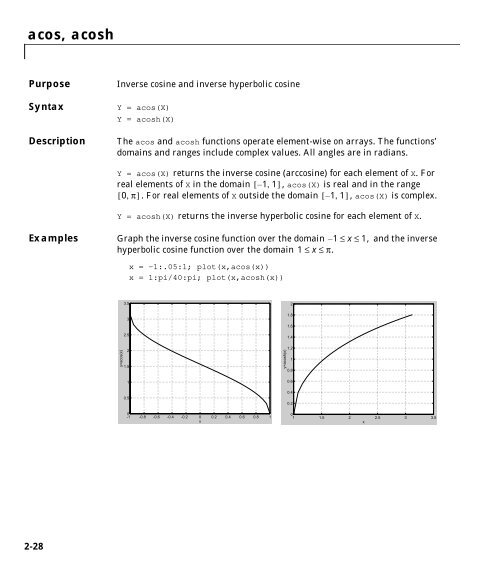
- Page 81: 2abs Purpose Absolute value and com
- Page 85 and 86: Algorithm acot and acoth use these
- Page 87 and 88: See Also csc, csch acsc, acsch 2-33
- Page 89 and 90: actxcontrol Note There are two ways
- Page 91 and 92: actxserver 2actxserver Purpose Crea
- Page 93 and 94: fig=figure; set(fig,'DoubleBuffer',
- Page 95 and 96: Verify that the files were added to
- Page 97 and 98: [W,ierr] = airy(k,Z) also returns a
- Page 99 and 100: 2all Purpose Test to determine if a
- Page 101 and 102: 2allchild Purpose Find all children
- Page 103 and 104: • 'rand' - set the AlphaData prop
- Page 105 and 106: 2alphamap Purpose Specify the figur
- Page 107 and 108: 2angle Purpose Phase angle Syntax P
- Page 109 and 110: 2any Purpose Test for any nonzeros
- Page 111 and 112: 2area Purpose Area fill of a two-di
- Page 113 and 114: 2asec, asech Purpose Inverse secant
- Page 115 and 116: 2asin, asinh Purpose Inverse sine a
- Page 117 and 118: 2assignin Purpose Assign a value to
- Page 119 and 120: 2atan, atanh Purpose Inverse tangen
- Page 121 and 122: 2atan2 Purpose Four-quadrant invers
- Page 123 and 124: 2audioplayer Purpose Create an audi
- Page 125 and 126: Property Description Type Type Name
- Page 127 and 128: Method Description audiorecorder is
- Page 129 and 130: audiorecorder Examples Example 1 Us
- Page 131 and 132: 2auwrite Purpose Write NeXT/SUN (.a
- Page 133 and 134:
Parameter Value Default You can als
- Page 135 and 136:
2aviinfo Purpose Return information
- Page 137 and 138:
2aviread Purpose Read an Audio Vide
- Page 139 and 140:
While the basic purpose of an axes
- Page 141 and 142:
In this example, the first plot occ
- Page 143 and 144:
Property Name Property Description
- Page 145 and 146:
Property Name Property Description
- Page 147 and 148:
Property Name Property Description
- Page 149 and 150:
Property Name Property Description
- Page 151 and 152:
Axes Properties objects in the axes
- Page 153 and 154:
CameraView Angle [0 1 0] (positive
- Page 155 and 156:
Color {none} | ColorSpec Axes Prope
- Page 157 and 158:
X-, Y-, Z-Limits following table de
- Page 159 and 160:
Axes Properties FontName A name suc
- Page 161 and 162:
Axes Properties When a handle’s v
- Page 163 and 164:
Axes Properties • replacechildren
- Page 165 and 166:
Axes Properties define object handl
- Page 167 and 168:
Visible {on} | off Axes Properties
- Page 169 and 170:
XMinorGrid, YMinorGrid, ZMinorGrido
- Page 171 and 172:
2axis Purpose Axis scaling and appe
- Page 173 and 174:
Examples The statements axis off tu
- Page 175 and 176:
5 4.5 4 3.5 3 2.5 2 1.5 1 0.5 axis(
- Page 177 and 178:
2balance Purpose Improve accuracy o
- Page 179 and 180:
Now the eigenvectors are well behav
- Page 181 and 182:
ar, barh distinct elements and show
- Page 183 and 184:
See Also bar3, ColorSpec, patch, st
- Page 185 and 186:
ar3, bar3h •'stacked' displays on
- Page 187 and 188:
See Also bar, LineSpec, patch 1 0.5
- Page 189 and 190:
2beep Purpose Produce a beep sound
- Page 191 and 192:
[H,ierr] = besselh(...) also return
- Page 193 and 194:
esseli, besselk and the other is a
- Page 195 and 196:
2besselj, bessely Purpose Bessel fu
- Page 197 and 198:
0.19602657795532 0.28670098806392 0
- Page 199 and 200:
1/168 1/252 1/360 1/495 1/660 In th
- Page 201 and 202:
Examples Example 1. bicg(afun,b,tol
- Page 203 and 204:
flag = relres = iter = 1 1 0 The va
- Page 205 and 206:
4559 This time U2 is nonsingular an
- Page 207 and 208:
time to precondition and converge t
- Page 209 and 210:
Example Example 1. bicgstab bicgsta
- Page 211 and 212:
icgstab flag2 is 0 because bicgstab
- Page 213 and 214:
2bin2dec Purpose Binary to decimal
- Page 215 and 216:
2bitcmp Purpose Complement bits Syn
- Page 217 and 218:
2bitmax Purpose Maximum floating-po
- Page 219 and 220:
2bitset Purpose Set bit Syntax C =
- Page 221 and 222:
2bitxor Purpose Bit-wise XOR Syntax
- Page 223 and 224:
2blkdiag Purpose Construct a block
- Page 225 and 226:
2break Purpose Terminate execution
- Page 227 and 228:
2builtin Purpose Execute builtin fu
- Page 229 and 230:
parameters Optional. A vector that
- Page 231 and 232:
function dydx = twoode(x,y) dydx =
- Page 233 and 234:
fprintf('The fourth eigenvalue is a
- Page 235 and 236:
2bvpget Purpose Extract properties
- Page 237 and 238:
solinit is a structure with the fol
- Page 239 and 240:
Property Value Description Vectoriz
- Page 241 and 242:
2calendar Purpose Calendar Syntax c
- Page 243 and 244:
camdolly Remarks camdolly sets the
- Page 245 and 246:
Examples This example creates a lig
- Page 247 and 248:
See Also campos, camtarget camlooka
- Page 249 and 250:
end camorbit Rotation in the camera
- Page 251 and 252:
2campos Purpose Set or query the ca
- Page 253 and 254:
2camproj Purpose Set or query the p
- Page 255 and 256:
2camtarget Purpose Set or query the
- Page 257 and 258:
2camup Purpose Set or query the cam
- Page 259 and 260:
2camva Purpose Set or query the cam
- Page 261 and 262:
2camzoom Purpose Zoom in and out on
- Page 263 and 264:
2cart2pol Purpose Transform Cartesi
- Page 265 and 266:
2case Purpose Case switch Descripti
- Page 267 and 268:
2catch Purpose Begin catch block De
- Page 269 and 270:
each time they render. CData values
- Page 271 and 272:
The blue color of the ocean is the
- Page 273 and 274:
2cdf2rdf Purpose Convert complex di
- Page 275 and 276:
2cdfinfo Purpose Return details abo
- Page 277 and 278:
Column 5 - Record and Dimension Var
- Page 279 and 280:
Examples Read all of the data from
- Page 281 and 282:
2cell Purpose Create cell array Syn
- Page 283 and 284:
2cell2struct Purpose Convert cell a
- Page 285 and 286:
2cellfun Purpose Apply a function t
- Page 287 and 288:
2cellplot Purpose Graphically displ
- Page 289 and 290:
2cgs Purpose Conjugate Gradients Sq
- Page 291 and 292:
Alternatively, use this matrix-vect
- Page 293 and 294:
2char Purpose Create character arra
- Page 295 and 296:
2checkin Purpose Check file into so
- Page 297 and 298:
2checkout Purpose Check file out of
- Page 299 and 300:
Example 2 - Check out Multiple File
- Page 301 and 302:
Destroy the positive definiteness (
- Page 303 and 304:
cholinc michol stands for modified
- Page 305 and 306:
0 20 40 60 80 100 120 140 0 50 nz =
- Page 307 and 308:
cholinc For hilb(20), the Cholesky
- Page 309 and 310:
2cholupdate Purpose Rank 1 update t
- Page 311 and 312:
Compare chol with cholupdate: R1 =
- Page 313 and 314:
2clabel Purpose Contour plot elevat
- Page 315 and 316:
2class Purpose Create object or ret
- Page 317 and 318:
2clc Purpose Clear Command Window G
- Page 319 and 320:
clear keyword clears the items indi
- Page 321 and 322:
To clear all compiled M- and MEX-fu
- Page 323 and 324:
2clf Purpose Clear current figure w
- Page 325 and 326:
2clock Purpose Current time as a da
- Page 327 and 328:
See Also delete, figure, gcf must s
- Page 329 and 330:
2closereq Purpose Default figure cl
- Page 331 and 332:
2colamd Purpose Column approximate
- Page 333 and 334:
2colmmd Purpose Sparse column minim
- Page 335 and 336:
See Also colamd, colperm, lu, sppar
- Page 337 and 338:
colorbar See Also colormap 10 8 6 4
- Page 339 and 340:
2colormap Purpose Set and get the c
- Page 341 and 342:
The rgbplot function plots colormap
- Page 343 and 344:
2ColorSpec Purpose Color specificat
- Page 345 and 346:
2colperm Purpose Sparse column perm
- Page 347 and 348:
2comet3 Purpose Three-dimensional c
- Page 349 and 350:
2compass Purpose Plot arrows emanat
- Page 351 and 352:
2complex Purpose Construct complex
- Page 353 and 354:
2computer Purpose Identify informat
- Page 355 and 356:
2cond Purpose Condition number with
- Page 357 and 358:
2condest Purpose 1-norm condition n
- Page 359 and 360:
coneplot(...,'method') specifies th
- Page 361 and 362:
3. Add the Slice Planes coneplot
- Page 363 and 364:
2conj Purpose Complex conjugate Syn
- Page 365 and 366:
2contour Purpose Two-dimensional co
- Page 367 and 368:
3 2.5 2 1.5 1 0.5 0 −0.5 −1 −
- Page 369 and 370:
2contour3 Purpose Three-dimensional
- Page 371 and 372:
2contourc Purpose Low-level contour
- Page 373 and 374:
2contourf Purpose Filled two-dimens
- Page 375 and 376:
2contourslice Purpose Draw contours
- Page 377 and 378:
3 2 1 0 −1 −2 −3 3 2 1 0 −1
- Page 379 and 380:
2conv Purpose Convolution and polyn
- Page 381 and 382:
In practice however, conv2 computes
- Page 383 and 384:
4 2 0 −2 −4 15 This figure comb
- Page 385 and 386:
2convhull Purpose Convex hull Synta
- Page 387 and 388:
2convhulln Purpose n-D convex hull
- Page 389 and 390:
2convn Purpose N-dimensional convol
- Page 391 and 392:
2copyobj Purpose Copy graphics obje
- Page 393 and 394:
2corrcoef Purpose Correlation coeff
- Page 395 and 396:
Algorithm cos and cosh use these al
- Page 397 and 398:
Algorithm cot and coth use these al
- Page 399 and 400:
2cplxpair Purpose Sort complex numb
- Page 401 and 402:
2cross Purpose Vector cross product
- Page 403 and 404:
Algorithm csc and csch use these al
- Page 405 and 406:
5 10 15 20 25 30 7 14 21 28 35 42 1
- Page 407 and 408:
2cumprod Purpose Cumulative product
- Page 409 and 410:
2cumtrapz Purpose Cumulative trapez
- Page 411 and 412:
2curl Purpose Computes the curl and
- Page 413 and 414:
See Also streamribbon, divergence c
- Page 415 and 416:
2cylinder Purpose Generate cylinder
- Page 417 and 418:
See Also sphere, surf 1 0.8 0.6 0.4
- Page 419 and 420:
daspect the window). This means set
- Page 421 and 422:
2date Purpose Current date string S
- Page 423 and 424:
Examples Convert a date string to a
- Page 425 and 426:
dateform (number) dateform (string)
- Page 427 and 428:
2datetick Purpose Label tick lines
- Page 429 and 430:
datetick('x',11) % Replace x-axis t
- Page 431 and 432:
ans = See Also clock, datenum, date
- Page 433 and 434:
See Also dbcont, dbdown, dbquit, db
- Page 435 and 436:
2dbdown Purpose Change local worksp
- Page 437 and 438:
dblquad The integrnd function integ
- Page 439 and 440:
2dbquit Purpose Quit debug mode Gra
- Page 441 and 442:
2dbstatus Purpose List all breakpoi
- Page 443 and 444:
2dbstop Purpose Set breakpoints in
- Page 445 and 446:
Examples The file buggy, used in th
- Page 447 and 448:
2dbtype Purpose List M-file with li
- Page 449 and 450:
2ddeadv Purpose Set up advisory lin
- Page 451 and 452:
2ddeexec Purpose Send string for ex
- Page 453 and 454:
2ddepoke Purpose Send data to appli
- Page 455 and 456:
2ddereq Purpose Request data from a
- Page 457 and 458:
2ddeterm Purpose Terminate DDE conv
- Page 459 and 460:
2deal Purpose Deal inputs to output
- Page 461 and 462:
2deblank Purpose Strip trailing bla
- Page 463 and 464:
2dec2bin Purpose Decimal to binary
- Page 465 and 466:
2deconv Purpose Deconvolution and p
- Page 467 and 468:
2del2 Purpose Discrete Laplacian Sy
- Page 469 and 470:
See Also diff, gradient V = 4*del2(
- Page 471 and 472:
Visualization Use one of these func
- Page 473 and 474:
1 0.5 0 −0.5 −1 15 delaunay Nex
- Page 475 and 476:
2delaunay3 Purpose 3-D Delaunay tes
- Page 477 and 478:
delaunay3 [2] National Science and
- Page 479 and 480:
3 9 1 5 2 9 1 6 2 3 9 4 2 3 9 1 7 9
- Page 481 and 482:
2delete Purpose Delete files or gra
- Page 483 and 484:
2delete (serial) Purpose Remove a s
- Page 485 and 486:
2depfun Purpose List the dependent
- Page 487 and 488:
depfun not examine the files on whi
- Page 489 and 490:
2det Purpose Matrix determinant Syn
- Page 491 and 492:
y = -0.0000 1.0000 -2.0000 1.0000 0
- Page 493 and 494:
2diag Purpose Diagonal matrices and
- Page 495 and 496:
2dialog Purpose Create and display
- Page 497 and 498:
2diff Purpose Differences and appro
- Page 499 and 500:
2dir Purpose Display directory list
- Page 501 and 502:
2disp Purpose Display text or array
- Page 503 and 504:
2display Purpose Overloaded method
- Page 505 and 506:
2divergence Purpose Computes the di
- Page 507 and 508:
2dlmread Purpose Read an ASCII deli
- Page 509 and 510:
2dmperm Purpose Dulmage-Mendelsohn
- Page 511 and 512:
2docopt Purpose Display location of
- Page 513 and 514:
To open the notepad editor and retu
- Page 515 and 516:
2double Purpose Convert to double-p
- Page 517 and 518:
2drawnow Purpose Complete pending d
- Page 519 and 520:
2dsearchn Purpose n-D nearest point
- Page 521 and 522:
2edit Purpose Edit or create M-file
- Page 523 and 524:
2eig Purpose Find eigenvalues and e
- Page 525 and 526:
Examples The matrix eigenvalues, it
- Page 527 and 528:
2eigs Purpose Find a few eigenvalue
- Page 529 and 530:
eigs(A,K,sigma,opts) and eigs(A,B,k
- Page 531 and 532:
[dum,ind] = sort(abs(d)); plot(dlm,
- Page 533 and 534:
(lambda - 4.0), where lambda is an
- Page 535 and 536:
2ellipj Purpose Jacobi elliptic fun
- Page 537 and 538:
2ellipke Purpose Complete elliptic
- Page 539 and 540:
2ellipsoid Purpose Generate ellipso
- Page 541 and 542:
2elseif Purpose Conditionally execu
- Page 543 and 544:
2end Purpose Terminate for, while,
- Page 545 and 546:
2eomday Purpose End of month Syntax
- Page 547 and 548:
2erf, erfc, erfcx, erfinv, erfcinv
- Page 549 and 550:
2error Purpose Display error messag
- Page 551 and 552:
errorbar(X,Y,E) 1.4 See Also LineSp
- Page 553 and 554:
displays this dialog box on a UNIX
- Page 555 and 556:
2etree Purpose Elimination tree Syn
- Page 557 and 558:
2eval Purpose Execute a string cont
- Page 559 and 560:
2evalc Purpose Evaluate MATLAB expr
- Page 561 and 562:
Limitation evalin cannot be used re
- Page 563 and 564:
If item is a Java class, then exist
- Page 565 and 566:
2exit Purpose Terminate MATLAB (sam
- Page 567 and 568:
2expint Purpose Exponential integra
- Page 569 and 570:
expm Notice that the diagonal eleme
- Page 571 and 572:
2ezcontour Purpose Easy to use cont
- Page 573 and 574:
ezcontour See Also contour, ezconto
- Page 575 and 576:
f( x, y) 31 ( - x) 2e x2 - ( y + 1)
- Page 577 and 578:
2ezmesh Purpose Easy to use 3-D mes
- Page 579 and 580:
2ezmeshc Purpose Easy to use combin
- Page 581 and 582:
2ezplot Purpose Easy to use functio
- Page 583 and 584:
2ezplot3 Purpose Easy to use 3-D pa
- Page 585 and 586:
2ezpolar Purpose Easy to use polar
- Page 587 and 588:
sqrt(x.^2 + y.^2); is written as: e
- Page 589 and 590:
2ezsurfc Purpose Easy to use combin
- Page 591 and 592:
See Also ezcontour, ezcontourf, ezm
- Page 593 and 594:
Symbols ! 2-22 - 2-10 % 2-22 & 2-20
- Page 595 and 596:
eta function (defined) 2-144 incomp
- Page 597 and 598:
colamd 2-277 colmmd 2-279 Color Axe
- Page 599 and 600:
dbclear 2-378 dbcont 2-380 dbdown 2
- Page 601 and 602:
ellipj 2-481 ellipke 2-483 elliptic
- Page 603 and 604:
help files, location for UNIX 2-457
- Page 605 and 606:
mldivide (M-file function equivalen
- Page 607 and 608:
sound files reading 2-76 writing 2-
- Page 609:
ZGrid, Axes property 2-114 ZLim, Ax