Online Model Selection Based on the Variational Bayes
Online Model Selection Based on the Variational Bayes
Online Model Selection Based on the Variational Bayes

Create successful ePaper yourself
Turn your PDF publications into a flip-book with our unique Google optimized e-Paper software.
LETTER Communicated by Hagai Attias<br />
<str<strong>on</strong>g>Online</str<strong>on</strong>g> <str<strong>on</strong>g>Model</str<strong>on</strong>g> <str<strong>on</strong>g>Selecti<strong>on</strong></str<strong>on</strong>g> <str<strong>on</strong>g>Based</str<strong>on</strong>g> <strong>on</strong> <strong>the</strong> Variati<strong>on</strong>al <strong>Bayes</strong><br />
Masa-aki Sato<br />
Informati<strong>on</strong> Sciences Divisi<strong>on</strong>, ATR Internati<strong>on</strong>al, and CREST, Japan Science and<br />
Tech<strong>on</strong>ology Corporati<strong>on</strong>, Seika-cho, Soraku-gun, Kyoto 619-0288, Japan<br />
The <strong>Bayes</strong>ian framework provides a principled way of model selecti<strong>on</strong>.<br />
This framework estimates a probability distributi<strong>on</strong> over an ensemble<br />
of models, and <strong>the</strong> predicti<strong>on</strong> is d<strong>on</strong>e by averaging over <strong>the</strong> ensemble of<br />
models. Accordingly, <strong>the</strong> uncertainty of <strong>the</strong> models is taken into account,<br />
and complex models with more degrees of freedom are penalized. However,<br />
integrati<strong>on</strong> over model parameters is often intractable, and some<br />
approximati<strong>on</strong> scheme is needed.<br />
Recently, a powerful approximati<strong>on</strong> scheme, called <strong>the</strong> variati<strong>on</strong>al<br />
bayes (VB) method, has been proposed. This approach de�nes <strong>the</strong> free<br />
energy for a trial probability distributi<strong>on</strong>, which approximates a joint posterior<br />
probability distributi<strong>on</strong> over model parameters and hidden variables.<br />
The exact maximizati<strong>on</strong> of <strong>the</strong> free energy gives <strong>the</strong> true posterior<br />
distributi<strong>on</strong>. The VB method uses factorized trial distributi<strong>on</strong>s. The integrati<strong>on</strong><br />
over model parameters can be d<strong>on</strong>e analytically, and an iterative<br />
expectati<strong>on</strong>-maximizati<strong>on</strong>-like algorithm, whose c<strong>on</strong>vergence is guaranteed,<br />
is derived.<br />
In this article, we derive an <strong>on</strong>line versi<strong>on</strong> of <strong>the</strong> VB algorithm and<br />
prove its c<strong>on</strong>vergence by showing that it is a stochastic approximati<strong>on</strong><br />
for �nding <strong>the</strong> maximum of <strong>the</strong> free energy. By combining sequential<br />
model selecti<strong>on</strong> procedures, <strong>the</strong> <strong>on</strong>line VB method provides a fully <strong>on</strong>line<br />
learning method with a model selecti<strong>on</strong> mechanism. In preliminary<br />
experiments using syn<strong>the</strong>tic data, <strong>the</strong> <strong>on</strong>line VB method was able to adapt<br />
<strong>the</strong> model structure to dynamic envir<strong>on</strong>ments.<br />
1 Introducti<strong>on</strong><br />
The learning of model parameters from observed data can be accomplished<br />
by using <strong>the</strong> maximum likelihood (ML) method for probabilistic models<br />
(Bishop, 1995). The expectati<strong>on</strong>-maximizati<strong>on</strong> (EM) algorithm (Dempster,<br />
Laird, & Rubin, 1977) provides a general framework for calculating <strong>the</strong> ML<br />
estimator for models with hidden variables. The fundamental problems of<br />
<strong>the</strong> ML method are over�tting and <strong>the</strong> inability to account for <strong>the</strong> model<br />
complexity, so it is unable to determine <strong>the</strong> model structure.<br />
The <strong>Bayes</strong>ian framework overcomes <strong>the</strong>se problems in principle (Bishop,<br />
1995; Cooper & Herskovitz, 1992; Gelman, Carlin, Stern, & Rubin, 1995;<br />
Neural Computati<strong>on</strong> 13, 1649–1681 (2001) c° 2001 Massachusetts Institute of Technology
1650 Masa-aki Sato<br />
Heckerman, Geiger, & Chickering, 1995; Mackay, 1992a, 1992b). The <strong>Bayes</strong>ian<br />
method estimates a probability distributi<strong>on</strong> over an ensemble of models,<br />
and <strong>the</strong> predicti<strong>on</strong> is d<strong>on</strong>e by averaging over <strong>the</strong> ensemble of models. Accordingly,<br />
<strong>the</strong> uncertainty of <strong>the</strong> models is taken into account, and complex<br />
models with more degrees of freedom are penalized. The evidence, which<br />
is <strong>the</strong> marginal posterior probability given <strong>the</strong> data, gives a criteri<strong>on</strong> for <strong>the</strong><br />
model selecti<strong>on</strong> (Mackay, 1992a, 1992b). However, an integrati<strong>on</strong> over model<br />
parameters is often intractable, and some approximati<strong>on</strong> scheme is needed<br />
(Chickering & Heckerman, 1997; Mackay, 1999; Neal, 1996; Richards<strong>on</strong> &<br />
Green, 1997;Roberts, Husmeier, Rezek, & Penny, 1998). Markov chain M<strong>on</strong>te<br />
Carlo (MCMC) methods and <strong>the</strong> Laplace approximati<strong>on</strong> method have been<br />
developed to date. MCMC methods can, in principle, �nd exact results,<br />
but <strong>the</strong>y require a huge amount of time for computati<strong>on</strong>. In additi<strong>on</strong>, it is<br />
dif�cult to determine when <strong>the</strong>se algorithms c<strong>on</strong>verge. The Laplace approximati<strong>on</strong><br />
method makes a local gaussian approximati<strong>on</strong> around a maximum<br />
a posteriori parameter estimate. This approximati<strong>on</strong> is valid <strong>on</strong>ly for a large<br />
sample limit. Unfortunately, it is not suited to parameters with c<strong>on</strong>straints<br />
such as mixing proporti<strong>on</strong>s of mixture models.<br />
Recently, an alternative approach, variati<strong>on</strong>al <strong>Bayes</strong> (VB), has been proposed<br />
(Waterhouse, Mackay, & Robins<strong>on</strong>, 1996; Attias, 1999, 2000; Ghahramani<br />
& Beal, 2000; Bishop, 1999). This approach de�nes <strong>the</strong> free energy<br />
for a trial probability distributi<strong>on</strong>, which approximates a joint posterior<br />
probability distributi<strong>on</strong> over model parameters and hidden variables. The<br />
maximum of <strong>the</strong> free energy gives <strong>the</strong> log evidence for an observed data set.<br />
Therefore, <strong>the</strong> exact maximizati<strong>on</strong> of <strong>the</strong> free energy gives <strong>the</strong> true posterior<br />
distributi<strong>on</strong> over <strong>the</strong> parameters and <strong>the</strong> hidden variables. The VB method<br />
uses trial distributi<strong>on</strong>s in a restricted space where <strong>the</strong> parameters are assumed<br />
to be c<strong>on</strong>diti<strong>on</strong>ally independent of <strong>the</strong> hidden variables. Once this<br />
approximati<strong>on</strong> is made, <strong>the</strong> remaining calculati<strong>on</strong>s are all d<strong>on</strong>e exactly. As<br />
a result, an iterative EM-like algorithm, whose c<strong>on</strong>vergence is guaranteed,<br />
is derived. The predictive distributi<strong>on</strong> is also calculated analytically.<br />
The VB method has several attractive features. The method requires <strong>on</strong>ly<br />
a modest amount of computati<strong>on</strong>al time, comparable to that of <strong>the</strong> EM algorithm.<br />
The <strong>Bayes</strong>ian informati<strong>on</strong> criteri<strong>on</strong> (BIC) (Schwartz, 1978) and <strong>the</strong><br />
minimum descripti<strong>on</strong> length (MDL) criteri<strong>on</strong> (Rissanen, 1987) for <strong>the</strong> model<br />
selecti<strong>on</strong> are obtained from <strong>the</strong> VB method in a large sample limit (Attias,<br />
1999). In this limit, <strong>the</strong> VB algorithm becomes equivalent to <strong>the</strong> ordinary EM<br />
algorithm. The VB method can be easily extended to <strong>the</strong> hierarchical <strong>Bayes</strong><br />
method. Sequential model selecti<strong>on</strong> procedures (Ghahramani & Beal, 2000;<br />
Ueda, 1999) have also been proposed by combining <strong>the</strong> VB method and <strong>the</strong><br />
split-and-merge algorithm (Ueda, Nakano, Ghahramani, & Hint<strong>on</strong>, 1999).<br />
In this article, we derive an <strong>on</strong>-line versi<strong>on</strong> of <strong>the</strong> VB algorithm and prove<br />
its c<strong>on</strong>vergence by showing that it is a stochastic approximati<strong>on</strong> for �nding<br />
<strong>the</strong> maximum of <strong>the</strong> free energy. We also prove that <strong>the</strong> VB algorithm<br />
is a gradient method with <strong>the</strong> inverse of <strong>the</strong> Fisher informati<strong>on</strong> matrix for
<str<strong>on</strong>g>Online</str<strong>on</strong>g> <str<strong>on</strong>g>Model</str<strong>on</strong>g> <str<strong>on</strong>g>Selecti<strong>on</strong></str<strong>on</strong>g> <str<strong>on</strong>g>Based</str<strong>on</strong>g> <strong>on</strong> <strong>the</strong> Variati<strong>on</strong>al <strong>Bayes</strong> 1651<br />
<strong>the</strong> posterior parameter distributi<strong>on</strong> as a coef�cient matrix. Namely, <strong>the</strong> VB<br />
method is a type of natural gradient method (Amari, 1998). By combining<br />
sequential model selecti<strong>on</strong> procedures, <strong>the</strong> <strong>on</strong>line VB algorithm provides<br />
a fully <strong>on</strong>line learning method with a model selecti<strong>on</strong> mechanism. It can<br />
be applied to real-time applicati<strong>on</strong>s. In preliminary experiments using syn<strong>the</strong>tic<br />
data, <strong>the</strong> <strong>on</strong>line VB method was able to adapt <strong>the</strong> model structure to<br />
dynamic envir<strong>on</strong>ments. We also found that <strong>the</strong> introducti<strong>on</strong> of a discount<br />
factor was crucial for a fast c<strong>on</strong>vergence of <strong>the</strong> <strong>on</strong>line VB method.<br />
We study <strong>the</strong> VB method for general exp<strong>on</strong>ential family models with<br />
hidden variables (EFH models) (Amari, 1985), although <strong>the</strong> VB method<br />
can be applied to more general graphical models (Attias, 1999). The use<br />
of <strong>the</strong> EFH models makes <strong>the</strong> calculati<strong>on</strong>s transparent. Moreover, <strong>the</strong> EFH<br />
models include a lot of interesting models such as normalized gaussian networks<br />
(Sato & Ishii, 2000), hidden Markov models (Rabiner, 1989), mixture<br />
of gaussian models (Roberts, Husmeier, Rezek, & Penny, 1998), mixture of<br />
factor analyzers (Ghahramani & Beal, 2000), mixture of probabilistic principal<br />
comp<strong>on</strong>ent analyzers (Tipping & Bishop, 1999), and o<strong>the</strong>rs (Roweis &<br />
Ghahramani, 1999; Titteringt<strong>on</strong>, Smith, & Makov, 1985).<br />
2 Variati<strong>on</strong>al <strong>Bayes</strong> Method<br />
In this secti<strong>on</strong>, we review <strong>the</strong> VB method (Waterhouse et al., 1996; Attias,<br />
1999, 2000; Ghahramani & Beal, 2000; Bishop, 1999) for EFH models (Amari,<br />
1985).<br />
2.1 <strong>Bayes</strong>ian Method. In <strong>the</strong> maximum likelihood (ML) approach, <strong>the</strong><br />
objective is to �nd <strong>the</strong> ML estimator that maximizes <strong>the</strong> likelihood for a<br />
given data set. The ML approach, however, suffers from over�tting and <strong>the</strong><br />
inability to determine <strong>the</strong> best model structure.<br />
In <strong>the</strong> <strong>Bayes</strong>ian method (Bishop, 1995; Mackay, 1992a, 1992b), a set of<br />
models, fMm |m D 1, . . . , N g, where Mm denotes a model with a �xed structure,<br />
is c<strong>on</strong>sidered. A probability distributi<strong>on</strong> for a model Mm with a model<br />
parameter µm is denoted by P(x| µm, Mm), where x represents an observed<br />
stochastic variable. For a set of observed data, XfTg D fx(t)|t D 1, . . . , Tg,<br />
and a prior probability distributi<strong>on</strong> P(µm |Mm), <strong>the</strong> <strong>Bayes</strong>ian method calculates<br />
<strong>the</strong> posterior probability over <strong>the</strong> parameter,<br />
P(µm|XfTg, Mm) D P(XfTg| µm, Mm)P(µm |Mm)<br />
.<br />
P(XfTg|Mm)<br />
Here, <strong>the</strong> data likelihood is de�ned by<br />
P(XfTg| µm, Mm) D<br />
TY<br />
P(x(t)| µm, Mm),<br />
tD1
1652 Masa-aki Sato<br />
and <strong>the</strong> evidence for a model Mm is de�ned by<br />
Z<br />
P(XfTg|Mm) D dm (µm)P(XfTg| µm, Mm)P(µm |Mm).<br />
The posterior probability over model structure is given by<br />
P(Mm |XfTg) D<br />
P(XfTg|Mm)P(Mm)<br />
P m0 P(XfTg|Mm0)P(Mm0) .<br />
If we use a n<strong>on</strong>informative prior for <strong>the</strong> model structure, that is, P(Mm) D<br />
1/N , <strong>the</strong> posterior for a given model P(Mm |XfTg) is proporti<strong>on</strong>al to <strong>the</strong> evidence<br />
of <strong>the</strong> model P(XfTg|Mm). Therefore, <strong>the</strong> model selecti<strong>on</strong> can be d<strong>on</strong>e<br />
according to <strong>the</strong> evidence. In <strong>the</strong> following, we will calculate <strong>the</strong> evidence<br />
for a given model by using <strong>the</strong> VB method, and <strong>the</strong> explicit model structure<br />
dependence is omitted.<br />
2.2 Exp<strong>on</strong>ential Family <str<strong>on</strong>g>Model</str<strong>on</strong>g> with Hidden Variables. An EFH model<br />
for an N-dimensi<strong>on</strong>al vector variable x D (x1, . . . , xN ) T is de�ned by a probability<br />
distributi<strong>on</strong>,<br />
Z<br />
P(x| µ ) D dm (z)P(x, z| µ ),<br />
P(x, z| µ ) D exp [r(x, z) ¢ µ C r0(x, z) ¡ Ã (µ )] , (2.1)<br />
where z D (z1, . . . , zM) T denotes an M-dimensi<strong>on</strong>al vector hidden variable<br />
and µ D (h1, . . . , hK) T denotes a set of model parameters called <strong>the</strong><br />
natural parameter. 1 A set of suf�cient statistics is denoted by r(x, z) D<br />
(r1(x, z), . . . , rK(x, z)) T . An inner product of two vectors r and µ is denoted<br />
by r ¢ µ D PK<br />
kD1 rkhk. Measures <strong>on</strong> <strong>the</strong> observed and <strong>the</strong> hidden variable<br />
spaces are denoted by dm (x) and dm (z), respectively. The normalizati<strong>on</strong> factor<br />
à (µ ) is determined by<br />
exp [Ã (µ )] D<br />
Z<br />
dm (x)dm (z) exp [r(x, z) ¢ µ C r0(x, z)] , (2.2)<br />
which is derived from <strong>the</strong> probability c<strong>on</strong>diti<strong>on</strong> R dm (x)P(x| µ ) D 1. P(x, z| µ )<br />
represents <strong>the</strong> probability distributi<strong>on</strong> for a complete event (x, z). If <strong>the</strong><br />
hidden variable is a discrete variable, <strong>the</strong> integrati<strong>on</strong> R dm (z) is replaced by<br />
<strong>the</strong> summati<strong>on</strong> P z .<br />
The expectati<strong>on</strong> parameter for <strong>the</strong> EFH model, Á D (w1, . . . , wK) T , is<br />
de�ned by<br />
Á D @Ã (µ )/@µ D (@Ã/@h1, . . . , @Ã/@hK) T<br />
Z<br />
D E [r(x, z)| µ] D dm (x)dm (z)r(x, z)P(x, z| µ ). (2.3)<br />
1 In general, <strong>the</strong> natural parameter is a functi<strong>on</strong> of ano<strong>the</strong>r model parameter Q: h D<br />
h (Q). The following discussi<strong>on</strong> can also be applied in this case.
<str<strong>on</strong>g>Online</str<strong>on</strong>g> <str<strong>on</strong>g>Model</str<strong>on</strong>g> <str<strong>on</strong>g>Selecti<strong>on</strong></str<strong>on</strong>g> <str<strong>on</strong>g>Based</str<strong>on</strong>g> <strong>on</strong> <strong>the</strong> Variati<strong>on</strong>al <strong>Bayes</strong> 1653<br />
2.3 Evidence and Free Energy. The evidence for a data set XfTg is de-<br />
�ned by<br />
Z<br />
P(XfTg) D dm (µ )P(XfTg| µ )P0(µ ), (2.4)<br />
where dm (µ ) denotes a measure <strong>on</strong> <strong>the</strong> model parameter space and P0(µ )<br />
denotes a prior distributi<strong>on</strong> for <strong>the</strong> model parameters. The integrati<strong>on</strong> over<br />
model parameters in equati<strong>on</strong> 2.4 penalizes complex models with more degrees<br />
of freedom (Bishop, 1995). This integrati<strong>on</strong>, however, is often dif�cult<br />
to perform. In order to evaluate this integrati<strong>on</strong>, <strong>the</strong> VB method introduces<br />
a trial probability distributi<strong>on</strong> Q(µ, ZfTg), which approximates <strong>the</strong> posterior<br />
probability distributi<strong>on</strong> over <strong>the</strong> model parameter µ and <strong>the</strong> hidden<br />
variables ZfTg D fz(t)|t D 1, . . . , Tg:<br />
P(µ, ZfTg|XfTg) D P(XfTg, ZfTg| µ )P0(µ )<br />
, (2.5)<br />
P(XfTg)<br />
where <strong>the</strong> probability distributi<strong>on</strong> for a complete data set (XfTg, ZfTg) is<br />
given by<br />
P(XfTg, ZfTg| µ ) D<br />
TY<br />
P(x(t), z(t)| µ ). (2.6)<br />
tD1<br />
The Kullback-Leibler (KL) divergence between <strong>the</strong> trial distributi<strong>on</strong> Q(µ,<br />
ZfTg) and <strong>the</strong> true posterior distributi<strong>on</strong> P(µ, ZfTg|XfTg) is given by<br />
Z<br />
KL(Q||P) D dm (µ )dm (ZfTg) Q(µ, ZfTg)<br />
� ´<br />
Q(µ, ZfTg)<br />
£ log<br />
P(µ, ZfTg|XfTg)<br />
D log P(XfTg) ¡ F(XfTg, Q), (2.7)<br />
where <strong>the</strong> free energy F(XfTg, Q) is de�ned by<br />
Z<br />
F(XfTg, Q) D dm (µ )dm (ZfTg) Q(µ, ZfTg)<br />
�<br />
P(XfTg, ZfTg| µ )P0(µ<br />
£ log<br />
)<br />
´<br />
] . (2.8)<br />
Q(µ, ZfTg)<br />
Therefore, <strong>the</strong> true posterior distributi<strong>on</strong> is obtained by maximizing <strong>the</strong> free<br />
energy with respect to <strong>the</strong> trial distributi<strong>on</strong> Q(µ, ZfTg). The maximum of<br />
<strong>the</strong> free energy is equal to <strong>the</strong> log evidence:<br />
log P(XfTg) D max F(XfTg, Q) ¸ F(XfTg, Q), (2.9)<br />
Q<br />
Equati<strong>on</strong> 2.9 implies that <strong>the</strong> lower bound for <strong>the</strong> log evidence can be evaluated<br />
by using some trial posterior distributi<strong>on</strong>s Q(µ, ZfTg).
1654 Masa-aki Sato<br />
2.4 Variati<strong>on</strong>al <strong>Bayes</strong> Algorithm. In <strong>the</strong> VB method, trial posterior distributi<strong>on</strong>s<br />
are assumed to be factorized as<br />
Q(µ, ZfTg) D Q h (µ )Qz(ZfTg). (2.10)<br />
The hidden variables are assumed to be c<strong>on</strong>diti<strong>on</strong>ally independent with <strong>the</strong><br />
model parameters given <strong>the</strong> data. We also assume that <strong>the</strong> prior distributi<strong>on</strong><br />
P0(µ ) is given by <strong>the</strong> c<strong>on</strong>jugate prior distributi<strong>on</strong>2 for <strong>the</strong> EFH model,<br />
equati<strong>on</strong> 2.1,<br />
P0(µ ) D exp [c 0(®0 ¢ µ ¡ Ã (µ )) ¡ © (®0, c 0)] , (2.11)<br />
where (®0, c 0) are prior hyperparameters. The normalizati<strong>on</strong> factor © (®0, c 0)<br />
is determined by<br />
Z<br />
exp [© (®0, c 0)] D<br />
dm (µ ) exp [c 0(®0 ¢ µ ¡ Ã (µ ))] . (2.12)<br />
Equati<strong>on</strong>s 2.10 and 2.11 are <strong>the</strong> <strong>on</strong>ly assumpti<strong>on</strong>s in this method. Under<br />
<strong>the</strong>se assumpti<strong>on</strong>s, we try to maximize <strong>the</strong> free energy F(XfTg, Q). The maximum<br />
free energy with respect to factorized Q, 2.10, gives an estimate (lower<br />
bound) for <strong>the</strong> log evidence log(P(XfTg)).<br />
The free energy can be maximized by alternately maximizing <strong>the</strong> free<br />
energy with respect to Qh and Qz. This process closely resembles <strong>the</strong> free<br />
energy formulati<strong>on</strong> for <strong>the</strong> EM algorithm (Neal & Hint<strong>on</strong>, 1998) for �nding<br />
<strong>the</strong> ML estimator. In <strong>the</strong> VB expectati<strong>on</strong> step (E-step), <strong>the</strong> free energy is maximized<br />
with respect to Qz(ZfTg) under <strong>the</strong> c<strong>on</strong>diti<strong>on</strong> R dm (ZfTg)Qz(ZfTg) D<br />
1, while Qh (µ ) is �xed. The maximum soluti<strong>on</strong> is given by <strong>the</strong> posterior<br />
distributi<strong>on</strong> for <strong>the</strong> hidden variables with <strong>the</strong> ensemble average of model<br />
parameters (see appendix A):<br />
Qz(ZfTg) D<br />
TY<br />
Qz(z(t)), (2.13)<br />
tD1<br />
Qz(z(t)) D P(z(t)|x(t), µ N ) D P(x(t), z(t)| µ N )/P(x(t)| µ N ),<br />
Z<br />
(2.14)<br />
Nµ D dm (µ )Qh (µ )µ. (2.15)<br />
In <strong>the</strong> VB maximizati<strong>on</strong> step (M-step), <strong>the</strong> free energy is maximized with<br />
respect to Qh (µ ) under <strong>the</strong> c<strong>on</strong>diti<strong>on</strong> R dm (µ )Qh (µ ) D 1, while Qz(ZfTg)<br />
obtained in <strong>the</strong> VB E-step is �xed. The maximum soluti<strong>on</strong> is given by <strong>the</strong><br />
2 It is also possible to use n<strong>on</strong>informative priors (Attias, 1999).
<str<strong>on</strong>g>Online</str<strong>on</strong>g> <str<strong>on</strong>g>Model</str<strong>on</strong>g> <str<strong>on</strong>g>Selecti<strong>on</strong></str<strong>on</strong>g> <str<strong>on</strong>g>Based</str<strong>on</strong>g> <strong>on</strong> <strong>the</strong> Variati<strong>on</strong>al <strong>Bayes</strong> 1655<br />
c<strong>on</strong>jugate distributi<strong>on</strong> for <strong>the</strong> EFH model with posterior hyperparameters<br />
(®, c ) (see appendix A):<br />
Q h (µ ) D P a (µ | ®, c ) D exp [c (® ¢ µ ¡ Ã (µ )) ¡ © (®, c )] , (2.16)<br />
c D T C c 0, (2.17)<br />
® D 1 h i<br />
Thr(x, z)i N C ®0 ¢ c 0 ,<br />
c µ<br />
(2.18)<br />
hr(x, z)i N D<br />
µ 1<br />
TX<br />
Z<br />
T<br />
dm (z(t))P(z(t)|x(t), µ N )r(x(t), z(t)). (2.19)<br />
tD1<br />
The effective amount of data c D (T C c 0) represents <strong>the</strong> reliability (or uncertainty)<br />
of <strong>the</strong> estimati<strong>on</strong>. As <strong>the</strong> amount of data T increases, <strong>the</strong> reliability<br />
of <strong>the</strong> estimati<strong>on</strong> increases. The prior hyperparameter c 0 represents <strong>the</strong> reliability<br />
of <strong>the</strong> prior belief <strong>on</strong> <strong>the</strong> prior hyperparameter ®0. The posterior<br />
hyperparameter ® is determined by <strong>the</strong> expectati<strong>on</strong> value of <strong>the</strong> suf�cient<br />
statistics. The prior hyperparameter ®0 gives <strong>the</strong> initial value for ®.<br />
Since <strong>the</strong> posterior parameter distributi<strong>on</strong> Qh (µ ) is given by <strong>the</strong> c<strong>on</strong>jugate<br />
distributi<strong>on</strong> Pa (µ | ®, c ), which is also an exp<strong>on</strong>ential family model, <strong>the</strong><br />
integrati<strong>on</strong> over <strong>the</strong> parameter µ in equati<strong>on</strong> 2.15 can be explicitly calculated<br />
as<br />
Nµ D hµi ® , (2.20)<br />
Z<br />
hµi ® D dm (µ )Pa (µ | ®, c )µ D 1 @©<br />
c @® (®, c ). (2.21)<br />
The natural parameter of <strong>the</strong> c<strong>on</strong>jugate distributi<strong>on</strong> is given by (c ®, c ). The<br />
corresp<strong>on</strong>ding expectati<strong>on</strong> parameters are given by <strong>the</strong> ensemble averages<br />
of <strong>the</strong> model parameters: hµi ® de�ned in equati<strong>on</strong> 2.21 and<br />
hà (µ )i ® D<br />
Z<br />
D 1<br />
c<br />
dm (µ )Pa (µ | ®, c )Ã (µ )<br />
@©<br />
@® (®, c ) ¢ ® ¡ @©<br />
@c (®, c ). (2.22)<br />
2.5 Parameterized Free Energy Functi<strong>on</strong>. Since <strong>the</strong> optimal soluti<strong>on</strong> simultaneously<br />
satis�es equati<strong>on</strong>s 2.14 and 2.16, <strong>the</strong> trial posterior distributi<strong>on</strong>s,<br />
Q h (µ ) and Qz(ZfTg), can be parameterized as<br />
Qh (µ ) D Pa (µ | ®, c ) D exp [c (® ¢ µ ¡ Ã (µ )) ¡ © (®, c )] , (2.23)<br />
TY<br />
Qz(ZfTg) D Qz(z(t)), (2.24)<br />
tD1<br />
Qz(z(t)) D P(z(t)|x(t), N µ ), (2.25)
1656 Masa-aki Sato<br />
where c , ®, and N µ are arbitrary variati<strong>on</strong>al parameters. By substituting this<br />
parameterized form into <strong>the</strong> de�niti<strong>on</strong> of <strong>the</strong> free energy, equati<strong>on</strong> 2.8, <strong>on</strong>e<br />
can get <strong>the</strong> parameterized free energy functi<strong>on</strong>:<br />
F(XfTg, N µ, ®, c ) D<br />
TX<br />
log P(x(t)| µ<br />
N ) C (c 0®0 ¡ c ® ) ¢ hµi ®<br />
tD1<br />
C Thr(x, z)i N µ ¢ (hµi ® ¡ N µ ) ¡ (T C c 0 ¡c )hà (µ )i ®<br />
C TÃ ( N µ ) C © (®, c ) ¡ © (®0, c 0), (2.26)<br />
where <strong>the</strong> ensemble averages of <strong>the</strong> parameters hµi ® and hà (µ )i ® are given<br />
by equati<strong>on</strong>s 2.21 and 2.22, respectively.<br />
The VB E-step equati<strong>on</strong>, 2.20, can be derived from <strong>the</strong> free energy maximizati<strong>on</strong><br />
c<strong>on</strong>diti<strong>on</strong> with respect to µ: N<br />
@F(XfTg, N µ, ®, c )/@ N µ D 0. (2.27)<br />
The derivative of <strong>the</strong> free energy with respect to N µ is given by (see appendix<br />
B)<br />
@F/@ N µ D U( N µ ) ¢ (hµi ® ¡ N µ ),<br />
U( N µ ) D<br />
TX<br />
tD1<br />
D± ²<br />
r(x(t), z(t)) ¡ hr(x(t), z(t))i Nµ<br />
£ ± r(x(t), z(t)) ¡ hr(x(t), z(t))i N<br />
µ<br />
Z<br />
,<br />
N<br />
µ<br />
hr(x(t), z(t))i N D<br />
µ<br />
dm (z(t))P(z(t)|x(t), µ N )r(x(t), z(t)). (2.28)<br />
Since <strong>the</strong> coef�cient matrix U is positive de�nite, <strong>the</strong> maximizati<strong>on</strong> c<strong>on</strong>diti<strong>on</strong>,<br />
equati<strong>on</strong> 2.27, leads to <strong>the</strong> VB E-step equati<strong>on</strong>, 2.20. The Hessian of<br />
<strong>the</strong> free energy with respect to N µ at <strong>the</strong> VB E-step soluti<strong>on</strong> is given by (¡U).<br />
This shows that <strong>the</strong> VB E-step soluti<strong>on</strong> is actually a maximum of <strong>the</strong> free<br />
energy with respect to N µ.<br />
The VB M-step equati<strong>on</strong>s, 2.17 and 2.18, can be derived from <strong>the</strong> free<br />
energy maximizati<strong>on</strong> c<strong>on</strong>diti<strong>on</strong> with respect to (®, c ):<br />
@F(XfTg, N µ, ®, c )/@c D 0,<br />
@F(XfTg, N µ, ®, c )/@® D 0. (2.29)<br />
The derivative of <strong>the</strong> free energy with respect to (®, c ) is given by (see<br />
²T ¾
<str<strong>on</strong>g>Online</str<strong>on</strong>g> <str<strong>on</strong>g>Model</str<strong>on</strong>g> <str<strong>on</strong>g>Selecti<strong>on</strong></str<strong>on</strong>g> <str<strong>on</strong>g>Based</str<strong>on</strong>g> <strong>on</strong> <strong>the</strong> Variati<strong>on</strong>al <strong>Bayes</strong> 1657<br />
appendix B)<br />
� 1<br />
c<br />
´ �<br />
(@F/@® ) V® ,® D<br />
(@F/@c )<br />
, V ® ,c<br />
V T<br />
® ,c ´<br />
, Vc ,c<br />
� ´<br />
Thr(x, z)i N C c 0®0 ¡ (T C c 0)®<br />
£ µ , (2.30)<br />
T C c 0 ¡ c<br />
where <strong>the</strong> Fisher informati<strong>on</strong> matrix V for <strong>the</strong> posterior parameter distributi<strong>on</strong><br />
P a (µ | ®, c ) is given by<br />
1<br />
V ® ,® D<br />
c 2<br />
½ � ´ �<br />
@ log Pa @ log Pa @® @® T<br />
´¾<br />
®<br />
D<br />
D (µ ¡ hµi ® )(µ ¡ hµi ® ) TE<br />
® ,<br />
V ® ,c D 1<br />
½ � ´ � ´¾<br />
@ log Pa @ log Pa c @® @c ®<br />
D « (µ ¡ hµi ® )(g(µ ) ¡ hg(µ )i ® )¬<br />
® ,<br />
½ � ´ � ´¾<br />
@ log Pa @ log Pa Vc ,c D<br />
@c @c ®<br />
D « (g(µ ) ¡ hg(µ )i ® )(g(µ ) ¡ hg(µ )i ® )¬<br />
® ,<br />
g(µ ) D ® ¢ µ ¡ Ã (µ ). (2.31)<br />
Since <strong>the</strong> Fisher informati<strong>on</strong> matrix V is positive de�nite, <strong>the</strong> free energy<br />
maximizati<strong>on</strong> c<strong>on</strong>diti<strong>on</strong>, 2.29, leads to <strong>the</strong> VB M-step equati<strong>on</strong>s, 2.17 and<br />
2.18. From equati<strong>on</strong> 2.30, it is shown that <strong>the</strong> VB M-step soluti<strong>on</strong> is a maximum<br />
of <strong>the</strong> free energy with respect to (®, c ), as in <strong>the</strong> VB-E step.<br />
The VB algorithm is summarized as follows. First, c is set to (T C c 0).<br />
In <strong>the</strong> VB E-step, <strong>the</strong> ensemble average of <strong>the</strong> parameter N µ is calculated by<br />
using equati<strong>on</strong> 2.20. Subsequently, <strong>the</strong> expectati<strong>on</strong> value of <strong>the</strong> suf�cient<br />
statistics hr(x, z)i N µ , 2.19, is calculated by using <strong>the</strong> posterior distributi<strong>on</strong> for<br />
<strong>the</strong> hidden variable P(z(t)|x(t), N µ ), equati<strong>on</strong> 2.14. In <strong>the</strong> VB M-step, <strong>the</strong> posterior<br />
hyperparameter ® is updated by using equati<strong>on</strong> 2.18. Repeating this<br />
process, <strong>the</strong> free energy functi<strong>on</strong>, equati<strong>on</strong> 2.26, increases m<strong>on</strong>ot<strong>on</strong>ically.<br />
This process c<strong>on</strong>tinues until <strong>the</strong> free energy functi<strong>on</strong> c<strong>on</strong>verges.<br />
Using equati<strong>on</strong>s 2.28 and 2.30, VB equati<strong>on</strong>s 2.20 and 2.18 can be expressed<br />
as <strong>the</strong> gradient method:<br />
D N µ D N µnew ¡ N µ D hµi ® ¡ N µ<br />
D U ¡1 ( µ<br />
N ) @F<br />
@N (XfTg,<br />
µ<br />
N µ, ®, c ), (2.32)
1658 Masa-aki Sato<br />
D® D ®new ¡ ® D 1<br />
c (Thr(x, z)i N C c 0®0 ¡c ®<br />
µ )<br />
D 1<br />
2<br />
V¡1<br />
c ® ,® (®, c ) @F<br />
@® (XfTg, N µ, ®, c ), (2.33)<br />
toge<strong>the</strong>r with c D T C c 0. Substituting <strong>the</strong> VB E-step equati<strong>on</strong>, 2.20, into <strong>the</strong><br />
free energy equati<strong>on</strong>, 2.26, <strong>the</strong> VB algorithm is fur<strong>the</strong>r rewritten as<br />
D® D 1<br />
V¡1<br />
2<br />
c ® ,® (®, c ) @F<br />
@® (XfTg, µ N D hµi ® , ®, c ). (2.34)<br />
This shows that <strong>the</strong> VB algorithm is <strong>the</strong> gradient method with <strong>the</strong> inverse of<br />
<strong>the</strong> Fisher informati<strong>on</strong> matrix as a coef�cient matrix. Namely, it is a type of<br />
natural gradient method (Amari, 1998), which gives <strong>the</strong> optimal asymptotic<br />
c<strong>on</strong>vergence. This fact is proved for <strong>the</strong> �rst time in this article. The natural<br />
gradient gives <strong>the</strong> steepest directi<strong>on</strong> in <strong>the</strong> hyperparameter space, which has<br />
<strong>the</strong> Riemannian structure according to <strong>the</strong> informati<strong>on</strong> geometry. It should<br />
be noted that <strong>the</strong> learning rate in <strong>the</strong> VB algorithm, 2.34, is automatically<br />
determined by <strong>the</strong> inverse of <strong>the</strong> Fisher informati<strong>on</strong> matrix.<br />
When <strong>the</strong> VB algorithm c<strong>on</strong>verges, <strong>the</strong> free energy equati<strong>on</strong>, 2.26, can be<br />
written in a simple form:<br />
Z<br />
F(XfTg) D log(P(XfTg| µ<br />
N )P0( µ<br />
N )) ¡<br />
dm (µ ) Qh (µ ) log(Qh (µ ))<br />
C c [Y( µ<br />
N ) ¡ hY(µ )i ® ]. (2.35)<br />
The �rst term <strong>on</strong> <strong>the</strong> right-hand side is <strong>the</strong> log likelihood toge<strong>the</strong>r with <strong>the</strong><br />
prior. It is estimated at <strong>the</strong> ensemble average of <strong>the</strong> parameters. The sec<strong>on</strong>d<br />
term is <strong>the</strong> entropy of <strong>the</strong> posterior parameter distributi<strong>on</strong>. It penalizes <strong>the</strong><br />
complex models and over�tting. The third term represents <strong>the</strong> deviati<strong>on</strong><br />
from <strong>the</strong> ensemble average of <strong>the</strong> parameters and becomes negligible in <strong>the</strong><br />
large sample limit.<br />
2.6 Predictive Distributi<strong>on</strong>. If <strong>the</strong> posterior parameter distributi<strong>on</strong> is<br />
obtained by using <strong>the</strong> VB algorithm, <strong>on</strong>e can calculate <strong>the</strong> predictive distributi<strong>on</strong><br />
for <strong>the</strong> observed variable x. The predictive distributi<strong>on</strong> for x is given<br />
by<br />
Z<br />
P(x|XfTg) D dm (µ )Qh (µ )P(x| µ )<br />
Z<br />
D<br />
dm (µ )<br />
Z<br />
dm (z) exp [(r(x, z) C c ® ) ¢ µ C r0(x, z)<br />
¡ (1 C c )Ã (µ ) ¡ © (®, c )] . (2.36)
<str<strong>on</strong>g>Online</str<strong>on</strong>g> <str<strong>on</strong>g>Model</str<strong>on</strong>g> <str<strong>on</strong>g>Selecti<strong>on</strong></str<strong>on</strong>g> <str<strong>on</strong>g>Based</str<strong>on</strong>g> <strong>on</strong> <strong>the</strong> Variati<strong>on</strong>al <strong>Bayes</strong> 1659<br />
By interchanging <strong>the</strong> integrati<strong>on</strong> with respect to µ and z, <strong>on</strong>e can get<br />
Z<br />
P(x|XfTg) D dm (z)<br />
£ exp £ r0(x, z) C © ( O® (x, z), c C 1) ¡ © (®, c ) ¤ , (2.37)<br />
O® (x, z) D (c ® C r(x, z))/(1 C c ).<br />
For a �nite T, this predictive distributi<strong>on</strong> has a different functi<strong>on</strong>al form<br />
from <strong>the</strong> model distributi<strong>on</strong> P(x| µ ), equati<strong>on</strong> 2.1.<br />
2.7 Large Sample Limit. When <strong>the</strong> amount of observed data becomes<br />
large (T À 1 : c À 1), <strong>the</strong> soluti<strong>on</strong> of <strong>the</strong> VB algorithm becomes <strong>the</strong> ML<br />
estimator (Attias, 1999). In this limit, <strong>the</strong> integrati<strong>on</strong> over <strong>the</strong> parameters<br />
with respect to <strong>the</strong> posterior parameter distributi<strong>on</strong> can be approximated<br />
by using a stati<strong>on</strong>ary point approximati<strong>on</strong>:<br />
Z<br />
exp [© (®, c )] D<br />
dm (µ ) exp [c (a ¢ µ ¡ Ã (µ ))]<br />
µ<br />
� exp c (a ¢ O µ ¡ Ã ( µ<br />
O ) ¡ 1<br />
2 log<br />
�<br />
�<br />
�<br />
�c @2Ã @µ@µ ( �<br />
µ<br />
O<br />
�<br />
) �<br />
� C O(1/c <br />
) , (2.38)<br />
where O µ is <strong>the</strong> maximum of <strong>the</strong> exp<strong>on</strong>ent ¡ ® ¢ µ ¡ Ã (µ )¢ , that is,<br />
@Ã<br />
@µ ( O µ ) D ®. (2.39)<br />
Therefore, © can be approximated as<br />
© (®, c ) � c (a ¢ O µ ¡ Ã ( µ<br />
O ) ¡ 1<br />
2 log<br />
�<br />
�<br />
�<br />
�c @2Ã @µ@µ ( �<br />
µ<br />
O<br />
�<br />
) �<br />
� C O(1/c ). (2.40)<br />
C<strong>on</strong>sequently, <strong>the</strong> ensemble average of <strong>the</strong> parameter N µ can be approximated<br />
as<br />
Nµ D 1<br />
c<br />
� 1<br />
c<br />
@©<br />
@® (®, c )<br />
@<br />
@® (c (® ¢ O µ ¡ Ã ( O µ ))) D O µ. (2.41)<br />
The relati<strong>on</strong>s 2.39 and 2.41 imply that <strong>the</strong> posterior hyperparameter ® is<br />
equal to <strong>the</strong> expectati<strong>on</strong> parameter of <strong>the</strong> EFH model, Á (see equati<strong>on</strong> 2.3)<br />
in this limit. Fur<strong>the</strong>rmore, equati<strong>on</strong>s 2.18, 2.39, and 2.41 are equivalent to <strong>the</strong>
1660 Masa-aki Sato<br />
ordinary EM algorithm for <strong>the</strong> EFH model. In a large sample limit, <strong>the</strong> data<br />
term is dominant over <strong>the</strong> model complexity term. C<strong>on</strong>sequently, <strong>the</strong> free<br />
energy maximizati<strong>on</strong> becomes equivalent to <strong>the</strong> likelihood maximizati<strong>on</strong>.<br />
Using equati<strong>on</strong>s 2.40 and 2.41, <strong>the</strong> free energy becomes<br />
F �<br />
TX<br />
tD1<br />
log P(x| N µ ) ¡ K<br />
2 logc<br />
¡ 1<br />
2 log<br />
�<br />
�@<br />
�<br />
�<br />
2 Ã<br />
@µ@µ ( �<br />
µ N<br />
�<br />
) �<br />
� C c 0(a0 ¢ µ N ¡ Ã ( µ N )) ¡ © (®0, c 0) C O(1/c ).<br />
(2.42)<br />
This expressi<strong>on</strong> coincides with <strong>the</strong> BIC/MDL criteria (Rissanen, 1987;<br />
Schwartz, 1978).<br />
The predictive distributi<strong>on</strong> P(x|XfTg) in this limit coincides with <strong>the</strong><br />
model distributi<strong>on</strong> using <strong>the</strong> ML estimator P(x| N µ ). This can be shown by<br />
using <strong>the</strong> following relati<strong>on</strong>s:<br />
O® (x, z) � ®<br />
C 1<br />
c (r(x, z) ¡ ® ) C O(1/c 2 ),<br />
© ( O® (x, z), r C 1) � © (®, c ) C 1<br />
c (r(x, z) ¡ @©<br />
® )<br />
@® (®, c ) C @©<br />
@c (®, c )<br />
3 <str<strong>on</strong>g>Online</str<strong>on</strong>g> Variati<strong>on</strong>al <strong>Bayes</strong> Method<br />
� © (®, c ) C r(x, z) ¢ N µ ¡ Ã ( N µ ).<br />
3.1 Expectati<strong>on</strong> Value of <strong>the</strong> Free Energy. In this secti<strong>on</strong>, we derive an<br />
<strong>on</strong>line versi<strong>on</strong> of <strong>the</strong> VB algorithm. The amount of data increases over time<br />
in <strong>the</strong> <strong>on</strong>line learning. Therefore, it is desirable to calculate <strong>the</strong> free energy<br />
corresp<strong>on</strong>ding to a �xed amount of data. For this purpose, let us de�ne an<br />
expectati<strong>on</strong> value of <strong>the</strong> log evidence for a �nite amount of data:<br />
E £ log P(XfTg) ¤<br />
r D<br />
Z<br />
dm (XfTg)r (XfTg)<br />
�Z<br />
£ log<br />
dm (µ )P(XfTg| µ )P0(µ )<br />
´<br />
, (3.1)<br />
where r represents an unknown probability distributi<strong>on</strong> for observed data.<br />
The corresp<strong>on</strong>ding VB free energy is given by<br />
Z<br />
E [F(XfTg, Qh, Qz)] r D T<br />
µZ<br />
£ E<br />
dm (µ )Qh (µ )<br />
dm (z)Qz(z) log ¡ P(x, z| µ )/Qz(z) ¢<br />
r
<str<strong>on</strong>g>Online</str<strong>on</strong>g> <str<strong>on</strong>g>Model</str<strong>on</strong>g> <str<strong>on</strong>g>Selecti<strong>on</strong></str<strong>on</strong>g> <str<strong>on</strong>g>Based</str<strong>on</strong>g> <strong>on</strong> <strong>the</strong> Variati<strong>on</strong>al <strong>Bayes</strong> 1661<br />
Z<br />
C dm (µ )Qh (µ ) log ¡ P0(µ )/Qh (µ )¢ . (3.2)<br />
The ratio (c 0/ T) determines <strong>the</strong> relative reliability between <strong>the</strong> observed<br />
data and <strong>the</strong> prior belief for <strong>the</strong> parameter distributi<strong>on</strong>. The expected free<br />
energy, equati<strong>on</strong> 3.2, can be estimated by<br />
� ´<br />
T Xt<br />
Z<br />
F(Xft g, Qzftg, Qh , T) D<br />
t<br />
tD1<br />
dm (µ )Q Z<br />
h (µ )<br />
£ log ¡ P(x(t), z(t)| µ )/Qz(z(t)) ¢<br />
Z<br />
C<br />
dm (z(t))Qz(z(t))<br />
dm (µ )Q h (µ ) log ¡ P0(µ )/Q h (µ )¢ , (3.3)<br />
where Qzftg D fQz(z(t))|t D 1, . . . , t g. Note that t represents <strong>the</strong> actual<br />
amount of observed data, and it increases over time while T is �xed. The estimati<strong>on</strong><br />
of <strong>the</strong> posterior distributi<strong>on</strong> Qz(z(t)) is inaccurate in <strong>the</strong> early stage<br />
of <strong>the</strong> <strong>on</strong>line learning and gradually becomes accurate as learning proceeds.<br />
However, <strong>the</strong> early inaccurate estimati<strong>on</strong>s and <strong>the</strong> later accurate estimati<strong>on</strong>s<br />
c<strong>on</strong>tribute to <strong>the</strong> free energy (see equati<strong>on</strong> 3.3) in equal weight. This might<br />
cause slow c<strong>on</strong>vergence of <strong>the</strong> learning process. Therefore, we introduce a<br />
time-dependent discount factor l(t) (0 · l(t) · 1, t D 2, 3, . . .) for forgetting<br />
<strong>the</strong> earlier inaccurate estimati<strong>on</strong> effects. Accordingly, a discounted free<br />
energy is de�ned by<br />
F l (Xft g, Qzft g, Q h , T) D Tg(t )<br />
Z<br />
£<br />
tX<br />
�tY tD1<br />
l(s)<br />
sDtC1<br />
dm (µ )Qh (µ )<br />
Z<br />
´<br />
dm (z(t))Qz(z(t))<br />
£ log ¡ P(x(t), z(t)| µ )/Qz(z(t)) ¢<br />
Z<br />
C<br />
where g(t ) represents a normalizati<strong>on</strong> c<strong>on</strong>stant:<br />
g(t ) D<br />
"<br />
tX �tY tD1<br />
l(s)<br />
sDtC1<br />
´#¡1<br />
dm (µ )Q h (µ ) log ¡ P0(µ )/Q h (µ )¢ , (3.4)<br />
. (3.5)<br />
3.2 <str<strong>on</strong>g>Online</str<strong>on</strong>g> Variati<strong>on</strong>al <strong>Bayes</strong> Algorithm. The <strong>on</strong>line VB algorithm can<br />
be derived from <strong>the</strong> successive maximizati<strong>on</strong> of <strong>the</strong> discounted free energy<br />
(see equati<strong>on</strong> 3.4). Let us assume that Qzft ¡1g D fQz(z(t))|t D 1, . . . , t ¡1g<br />
(µ ) have been determined for an observed data set Xft ¡ 1g D<br />
and Q (t ¡1)<br />
h
1662 Masa-aki Sato<br />
fx(t)|t D 1, . . . , t ¡ 1g. With new observed data x(t ), <strong>the</strong> discounted free<br />
energy Fl (Xft g, Qzftg, Qh , T) is maximized with respect to Qz(z(t )), while<br />
Qh is set to Q (t ¡1)<br />
(µ ). The soluti<strong>on</strong> is given by<br />
h<br />
Qz(z(t )) D P(z(t )|x(t ), N µ (t ))<br />
µ<br />
N (t<br />
Z<br />
) D<br />
dm (µ )Q(t ¡1)<br />
(µ h<br />
)µ. (3.6)<br />
In <strong>the</strong> next step, <strong>the</strong> discounted free energy F l(Xft g, Qzftg, Q h , T) is maximized<br />
with respect to Q h (µ ), while Qzft g is �xed. The soluti<strong>on</strong> is given<br />
by<br />
Q (t )<br />
h (µ ) D exp [c (® (t ) ¢ µ ¡ Ã (µ )) ¡ © (® (t ), c )] ,<br />
c D T C c 0,<br />
c ® (t ) D Thhr(x, z)ii(t ) C c 0®0, (3.7)<br />
where <strong>the</strong> discounted average hh¢ii(t ) is de�ned by<br />
hhr(x, z)ii(t ) D g(t )<br />
Z<br />
£<br />
tX<br />
�tY tD1<br />
l(s)<br />
sDtC1<br />
´<br />
dm (z(t))Qz(z(t))r(x(t), z(t)). (3.8)<br />
The discounted average can be calculated by using a step-wise equati<strong>on</strong>:<br />
hhr(x, z)ii(t ) D (1 ¡ g(t ))hhr(x, z)ii(t ¡ 1)<br />
h<br />
C g(t )Ez r(x(t ), z(t ))| µ<br />
N (t ) i<br />
,<br />
g(t ) D (1 C l(t )/g(t ¡ 1)) ¡1 . (3.9)<br />
By using equati<strong>on</strong> 3.6, <strong>the</strong> expectati<strong>on</strong> value of <strong>the</strong> suf�cient statistics for<br />
<strong>the</strong> current data Ez[r(x(t ), z(t ))| N µ (t )] is given by<br />
Ez<br />
h<br />
r(x(t ), z(t ))| µ<br />
N (t ) i Z<br />
D dm (z(t ))<br />
£ P(z(t )|x(t ), N µ (t ))r(x(t ), z(t )). (3.10)<br />
The recursive formula for ® (t ) is derived from <strong>the</strong> above equati<strong>on</strong>s:<br />
D® (t ) D ® (t ) ¡ ® (t ¡ 1)
<str<strong>on</strong>g>Online</str<strong>on</strong>g> <str<strong>on</strong>g>Model</str<strong>on</strong>g> <str<strong>on</strong>g>Selecti<strong>on</strong></str<strong>on</strong>g> <str<strong>on</strong>g>Based</str<strong>on</strong>g> <strong>on</strong> <strong>the</strong> Variati<strong>on</strong>al <strong>Bayes</strong> 1663<br />
D 1<br />
c g(t ) ± h<br />
TEz r(x(t ), z(t ))| µ N (t ) i<br />
C c 0®0 ¡ c ® (t ¡ 1) ² . (3.11)<br />
By using equati<strong>on</strong> 3.7, <strong>the</strong> ensemble average of <strong>the</strong> parameter N µ (t ) de�ned<br />
in equati<strong>on</strong> 3.6 can be calculated as<br />
µ<br />
N (t ) D hµi ® (t ¡1) D 1 @©<br />
c @® (® (t ¡ 1), c ). (3.12)<br />
The <strong>on</strong>line VB algorithm is summarized as follows. In <strong>the</strong> VB E-step, <strong>the</strong><br />
ensemble average of <strong>the</strong> parameter N µ (t ) is determined by equati<strong>on</strong> 3.12. Using<br />
this value, <strong>on</strong>e calculates <strong>the</strong> expectati<strong>on</strong> value of <strong>the</strong> suf�cient statistics<br />
(see equati<strong>on</strong> 3.10) for <strong>the</strong> current data. The posterior hyperparameter ® (t )<br />
is updated by equati<strong>on</strong> 3.11 in <strong>the</strong> VB M-step. This process is repeated when<br />
new data are observed. By combining <strong>the</strong> VB E-step (3.12) and VB M-step<br />
(3.11) equati<strong>on</strong>s, <strong>on</strong>e can get <strong>the</strong> recursive update equati<strong>on</strong> for ® (t ):<br />
D® (t ) D 1<br />
c g(t<br />
�<br />
£<br />
) TEz r(x(t ), z(t ))|hh i ® (t ¡1) ¤<br />
C c 0®0 ¡ c ® (t ¡ 1)<br />
´<br />
. (3.13)<br />
3.3 Stochastic Approximati<strong>on</strong>. Unlike <strong>the</strong> VB algorithm, <strong>the</strong> discounted<br />
free energy in <strong>the</strong> <strong>on</strong>line VB algorithm does not always increase, because<br />
a new c<strong>on</strong>tributi<strong>on</strong> is added to <strong>the</strong> discounted free energy at each time<br />
instance. In <strong>the</strong> following, we prove that <strong>the</strong> <strong>on</strong>line VB algorithm can be<br />
c<strong>on</strong>sidered as a stochastic approximati<strong>on</strong> (Kushner & Yin, 1997) for �nding<br />
<strong>the</strong> maximum of <strong>the</strong> expected free energy de�ned in equati<strong>on</strong> 3.2, which<br />
gives a lower bound for <strong>the</strong> expected log evidence de�ned in equati<strong>on</strong> 3.1.<br />
The expected free energy (see equati<strong>on</strong> 3.2), in which <strong>the</strong> maximizati<strong>on</strong> with<br />
respect to Qz has been performed, can be written as<br />
where<br />
max E [F(XfTg, Qh , Qz)] r D E [FM(x, ®, T)] r , (3.14)<br />
Qz<br />
Z<br />
FM(x, ®, T) D T<br />
Z<br />
£<br />
dm (z)P(z|x, hµi ® )<br />
dm (µ )Q h (µ ) log ¡ P(x, z| µ )/P(z|x, hµi ® ) ¢
1664 Masa-aki Sato<br />
Z<br />
C<br />
The gradient of FM is calculated as<br />
dm (µ )Qh (µ ) log ¡ P0(µ )/Q h (µ )¢<br />
D T log P(x|hµi ® ) C © (®, c ) ¡ © (®0, c 0)<br />
¡ [(c ® ¡c 0®0) ¢ hµi ® ¡ TÃ (hµi ® )] (3.15)<br />
@FM<br />
@® (x, ®, T) D c V ® ,® (®, c )<br />
£ ¡ TEz [r(x, z)|hµi ® ] C c 0®0 ¡ c ® ¢ , (3.16)<br />
where <strong>the</strong> Fisher informati<strong>on</strong> matrix V ® ,® for <strong>the</strong> posterior parameter distributi<strong>on</strong>,<br />
Qh (µ ) D Pa (µ | ®, c ), is de�ned in equati<strong>on</strong> 2.31. C<strong>on</strong>sequently,<br />
<strong>the</strong> <strong>on</strong>line VB algorithm, 3.13, can be written as<br />
D® (t ) D 1<br />
c 2g(t )V ¡1<br />
® ,® (® (t ¡ 1), c ) ¢ @FM<br />
@® (x(t ), ® (t ¡ 1), T). (3.17)<br />
If <strong>the</strong> effective learning rate g(t )(¸ 0) satis�es <strong>the</strong> c<strong>on</strong>diti<strong>on</strong> (Kushner &<br />
Yin, 1997)<br />
1X<br />
g(t ) D 1 and<br />
tD1<br />
1X<br />
g<br />
tD1<br />
2 (t ) < 1, (3.18)<br />
<strong>the</strong> <strong>on</strong>line VB algorithm, equati<strong>on</strong> 3.13, de�nes <strong>the</strong> stochastic approximati<strong>on</strong><br />
for �nding <strong>the</strong> maximum of <strong>the</strong> expected free energy (see equati<strong>on</strong> 3.2).<br />
When <strong>the</strong>re is no discount factor, that is, l(t ) D 1, <strong>the</strong> effective learning<br />
rate g(t ) is given by<br />
g(t ) D 1/t. (3.19)<br />
This satis�es <strong>the</strong> stochastic approximati<strong>on</strong> c<strong>on</strong>diti<strong>on</strong>, equati<strong>on</strong> 3.18. However,<br />
<strong>the</strong> learning speed becomes very slow if this schedule is adopted (see<br />
secti<strong>on</strong> 5). The reas<strong>on</strong> for this slow c<strong>on</strong>vergence is that earlier inaccurate<br />
hyperparameter estimati<strong>on</strong>s affect <strong>the</strong> hyperparameter estimati<strong>on</strong>s in later<br />
learning stages because <strong>the</strong>re is no discount factor in <strong>the</strong> suf�cient statistics<br />
average (see equati<strong>on</strong> 3.8). The introducti<strong>on</strong> of <strong>the</strong> discount factor is crucial<br />
for fast c<strong>on</strong>vergence.<br />
As in <strong>the</strong> <strong>on</strong>line EM algorithm we proposed previously (Sato, 2000), we<br />
employ <strong>the</strong> following discount schedule,<br />
1 ¡ l(t ) D<br />
1<br />
, (3.20)<br />
(t ¡ 2)k C t0
<str<strong>on</strong>g>Online</str<strong>on</strong>g> <str<strong>on</strong>g>Model</str<strong>on</strong>g> <str<strong>on</strong>g>Selecti<strong>on</strong></str<strong>on</strong>g> <str<strong>on</strong>g>Based</str<strong>on</strong>g> <strong>on</strong> <strong>the</strong> Variati<strong>on</strong>al <strong>Bayes</strong> 1665<br />
which can be calculated recursively:<br />
l(t ) D 1 ¡<br />
1 ¡ l(t ¡ 1)<br />
. (3.21)<br />
1 C k (1 ¡ l(t ¡ 1))<br />
The corresp<strong>on</strong>ding effective learning rate g(t ) satis�es<br />
� ´<br />
k C 1 1<br />
g(t ) ¡!<br />
, (3.22)<br />
t !1 k t<br />
so that <strong>the</strong> stochastic approximati<strong>on</strong> c<strong>on</strong>diti<strong>on</strong> (see equati<strong>on</strong> 3.18) is satis-<br />
�ed. The c<strong>on</strong>stants appearing in equati<strong>on</strong> 3.20 have clear physical meanings.<br />
t0 represents how many samples c<strong>on</strong>tribute to <strong>the</strong> discounted average for<br />
<strong>the</strong> suf�cient statistics (see equati<strong>on</strong> 3.8) in <strong>the</strong> early stage of learning. k<br />
c<strong>on</strong>trols <strong>the</strong> asymptotic decreasing ratio for <strong>the</strong> effective learning c<strong>on</strong>stant<br />
g(t ), as in equati<strong>on</strong> 3.22. The values of t0 and k c<strong>on</strong>trol <strong>the</strong> learning speeds<br />
in <strong>the</strong> early and later stages of learning, respectively.<br />
3.4 Discussi<strong>on</strong>. There are some comments <strong>on</strong> our <strong>on</strong>line VB method.<br />
The objective functi<strong>on</strong> of our <strong>on</strong>line VB method is <strong>the</strong> expected log evidence<br />
(see equati<strong>on</strong> 3.1) for a �xed amount of data. Unlike <strong>the</strong> usual <strong>Bayes</strong>ian<br />
method, our <strong>on</strong>line VB method estimates <strong>the</strong> same quantity even if <strong>the</strong><br />
amount of <strong>the</strong> observed data is increased. The observed data are used for<br />
improving <strong>the</strong> estimati<strong>on</strong> quality of <strong>the</strong> expected free energy (see equati<strong>on</strong><br />
3.2) which approximates <strong>the</strong> expected log evidence (see equati<strong>on</strong> 3.1).<br />
Therefore, our <strong>on</strong>line VB method does not c<strong>on</strong>verge to <strong>the</strong> EM algorithm in<br />
<strong>the</strong> large sample limit (t ! 1 and T : �xed). Never<strong>the</strong>less, <strong>the</strong> method can<br />
perform both learning and predicti<strong>on</strong> c<strong>on</strong>currently in an <strong>on</strong>line fashi<strong>on</strong>.<br />
The batch VB method can be derived from our <strong>on</strong>line VB method if<br />
<strong>the</strong> same data set is repeatedly presented. Let suppose that <strong>the</strong> posterior<br />
hyperparameters are updated <strong>on</strong>ly at <strong>the</strong> end of each epoch, in which all<br />
of <strong>the</strong> data are presented <strong>on</strong>ce, by using equati<strong>on</strong> 3.7, while <strong>the</strong> discounted<br />
averages are calculated every time by using equati<strong>on</strong> 3.9. If <strong>the</strong> discount<br />
factor is given by l(t ) D 0 at <strong>the</strong> beginning of each epoch, or l(t ) D 1<br />
o<strong>the</strong>rwise, <strong>the</strong>n this <strong>on</strong>line VB method is equivalent to <strong>the</strong> batch VB method.<br />
It is also possible to use <strong>the</strong> log evidence for <strong>the</strong> observed data as in <strong>the</strong><br />
usual <strong>Bayes</strong>ian method. The corresp<strong>on</strong>ding <strong>on</strong>line VB algorithm can be derived<br />
by equating <strong>the</strong> amount of data t to T in equati<strong>on</strong> 3.3. In this case, <strong>the</strong><br />
objective functi<strong>on</strong> changes over time as <strong>the</strong> amount of data increases. The<br />
target posterior parameter distributi<strong>on</strong> also changes over time. The variance<br />
of <strong>the</strong> posterior parameter distributi<strong>on</strong> is proporti<strong>on</strong>al to 1/t. This gives too<br />
much c<strong>on</strong>�dence for <strong>the</strong> posterior parameter distributi<strong>on</strong> because <strong>the</strong> free<br />
energy is not fully maximized for each datum; that is, <strong>the</strong> VB-E and VB-M<br />
steps are performed <strong>on</strong>ce for each datum. C<strong>on</strong>sequently, this type of <strong>on</strong>line<br />
VB method so<strong>on</strong> c<strong>on</strong>verges to <strong>the</strong> EM algorithm: <strong>the</strong> posterior parameter
1666 Masa-aki Sato<br />
distributi<strong>on</strong> becomes sharply peaked near <strong>the</strong> maximum likelihood estimator.<br />
In order to avoid this dif�culty, <strong>the</strong> VB-E and VB-M steps should be<br />
iterated until c<strong>on</strong>vergence for each datum. However, <strong>the</strong> above algorithm<br />
is not an <strong>on</strong>line algorithm in usual sense.<br />
4 <str<strong>on</strong>g>Online</str<strong>on</strong>g> <str<strong>on</strong>g>Model</str<strong>on</strong>g> <str<strong>on</strong>g>Selecti<strong>on</strong></str<strong>on</strong>g><br />
In <strong>the</strong> usual <strong>Bayes</strong>ian procedure for model selecti<strong>on</strong>, <strong>on</strong>e prepares a set of<br />
models with different structures and calculates <strong>the</strong> evidence for each model.<br />
Then <strong>the</strong> best model that gives <strong>the</strong> highest evidence is selected or <strong>the</strong> average<br />
over models with different structures is taken. An alternative approach is to<br />
change model structure sequentially. Sequential model selecti<strong>on</strong> procedures<br />
have been proposed based <strong>on</strong> ei<strong>the</strong>r <strong>the</strong> batch VB method (Ghahramani &<br />
Beal, 2000; Ueda, 1999) or <strong>the</strong> MCMC method (Richards<strong>on</strong> & Green, 1997).<br />
In this article, we adopt sequential model selecti<strong>on</strong> procedures based <strong>on</strong><br />
<strong>the</strong> <strong>on</strong>line VB method. We can c<strong>on</strong>sider several sequential model selecti<strong>on</strong><br />
strategies. In <strong>the</strong> �rst method, we start from an initial model with a given<br />
structure. The VB learning process for this model is c<strong>on</strong>tinued by m<strong>on</strong>itoring<br />
<strong>the</strong> free energy value. When <strong>the</strong> free energy c<strong>on</strong>verges, <strong>the</strong> model structure<br />
is changed according to some criteri<strong>on</strong>, and <strong>the</strong> initial model is saved as<br />
<strong>the</strong> base model. The VB learning process for <strong>the</strong> current model is c<strong>on</strong>tinued<br />
until <strong>the</strong> free energy c<strong>on</strong>verges. If <strong>the</strong> free energy of <strong>the</strong> current model is<br />
greater than that of <strong>the</strong> base model, <strong>the</strong> current model is saved as <strong>the</strong> base<br />
model. O<strong>the</strong>rwise <strong>the</strong> base model is not changed. One always keeps <strong>the</strong> base<br />
model as <strong>the</strong> best model to date. A new trial model is selected based <strong>on</strong> <strong>the</strong><br />
base model. This process c<strong>on</strong>tinues until fur<strong>the</strong>r attempts do not improve<br />
<strong>the</strong> base model.<br />
The above procedure is a deterministic process. We can c<strong>on</strong>sider a stochastic<br />
model selecti<strong>on</strong> process based <strong>on</strong> <strong>the</strong> Metropolis algorithm (Metropolis,<br />
Rosenbluth, Rosenbluth, Teller, & Teller, 1953). In this case, <strong>the</strong> base model<br />
is different from <strong>the</strong> best model to date. If <strong>the</strong> free energy of <strong>the</strong> current<br />
model is greater than that of <strong>the</strong> base model, <strong>the</strong> current model is saved as<br />
<strong>the</strong> base model. O<strong>the</strong>rwise <strong>the</strong> base model is changed to <strong>the</strong> current model<br />
with <strong>the</strong> probability exp(b (Fcurrent ¡ Fbase)). This stochastic process can be<br />
applied to model selecti<strong>on</strong> in dynamic envir<strong>on</strong>ments.<br />
We also propose an <strong>on</strong>line model selecti<strong>on</strong> procedure using a hierarchical<br />
mixture of models with different structures. We train <strong>the</strong>m c<strong>on</strong>currently by<br />
using <strong>the</strong> <strong>on</strong>line VB method for each model. They are trained independently<br />
with each o<strong>the</strong>r. (It is also possible to train <strong>the</strong>m competitively by using <strong>the</strong><br />
<strong>on</strong>line VB method for <strong>the</strong> hierarchical mixture of models.) When <strong>the</strong> free<br />
energies c<strong>on</strong>verge, <strong>the</strong>se models are compared according to <strong>the</strong>ir free energy<br />
values. Then <strong>the</strong> current best model structure is selected. Structures of <strong>the</strong><br />
o<strong>the</strong>r models are changed based <strong>on</strong> <strong>the</strong> current best model structure. This<br />
sequential model selecti<strong>on</strong> procedure is suitable for dynamic envir<strong>on</strong>ment.
<str<strong>on</strong>g>Online</str<strong>on</strong>g> <str<strong>on</strong>g>Model</str<strong>on</strong>g> <str<strong>on</strong>g>Selecti<strong>on</strong></str<strong>on</strong>g> <str<strong>on</strong>g>Based</str<strong>on</strong>g> <strong>on</strong> <strong>the</strong> Variati<strong>on</strong>al <strong>Bayes</strong> 1667<br />
This method is used in a model selecti<strong>on</strong> task for dynamic envir<strong>on</strong>ments in<br />
secti<strong>on</strong> 5.<br />
In <strong>the</strong> next secti<strong>on</strong>, we study <strong>the</strong> model selecti<strong>on</strong> problem for mixture<br />
of gaussian models. As a mechanism for structural change, we adopt <strong>the</strong><br />
split-and-merge method proposed by Ueda et al. (1999) (see also Richards<strong>on</strong><br />
& Green, 1997; Ghahramani & Beal, 2000; Ueda, 1999). For mixture models,<br />
<strong>the</strong> split-and-merge method provides a simple procedure for structural<br />
changes. We choose ei<strong>the</strong>r to split a unit into two or to merge two units<br />
into <strong>on</strong>e in <strong>the</strong> sequential model selecti<strong>on</strong> process. In <strong>the</strong> current implementati<strong>on</strong>,<br />
<strong>the</strong> same process is applied if <strong>the</strong> previous attempt was successful.<br />
O<strong>the</strong>rwise <strong>the</strong> o<strong>the</strong>r process is applied.<br />
A criteri<strong>on</strong> for splitting a unit is given by <strong>the</strong> unit’s free energy, which is<br />
assigned to each unit (see appendix C). The split is applied to <strong>the</strong> unit with<br />
<strong>the</strong> lowest free energy am<strong>on</strong>g unattempted units. A criteri<strong>on</strong> for merging<br />
units is given by <strong>the</strong> correlati<strong>on</strong> between <strong>the</strong> two units’ activities, which are<br />
represented by <strong>the</strong> posterior probability that <strong>the</strong> units will be selected for<br />
given data. The unit pair with <strong>the</strong> highest correlati<strong>on</strong> am<strong>on</strong>g unattempted<br />
unit pairs is selected for merging. The deleti<strong>on</strong> of units is also performed<br />
for units with very small activities, which indicate that <strong>the</strong> units have not<br />
been selected at all.<br />
We adopted <strong>the</strong> above model selecti<strong>on</strong> procedure because of its simplicity.<br />
O<strong>the</strong>r model selecti<strong>on</strong> procedures using <strong>the</strong> split-and-merge algorithm<br />
have also been proposed (Ghahramani & Beal, 2000; Ueda, 1999).<br />
By combining <strong>the</strong> sequential model selecti<strong>on</strong> procedure with <strong>the</strong> <strong>on</strong>line<br />
VB learning method, a fully <strong>on</strong>line learning method with a model selecti<strong>on</strong><br />
mechanism is obtained, and it can be applied to real-time applicati<strong>on</strong>s.<br />
5 Experiments<br />
As a preliminary study <strong>on</strong> <strong>the</strong> performance of <strong>the</strong> <strong>on</strong>line VB method, we c<strong>on</strong>sidered<br />
model selecti<strong>on</strong> problems for two-dimensi<strong>on</strong>al mixture of gaussian<br />
(MG) models (see appendix C). We borrowed two tasks from Roberts et al.<br />
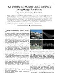
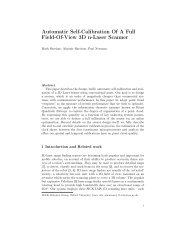
(1998). Data set A, c<strong>on</strong>sisting of 200 points, was generated from a mixture<br />
of four gaussians with <strong>the</strong> centers (0, 0), (2, p 12), (4, 0), and (¡2, ¡ p 12)<br />
(see Figure 1A). The gaussians had <strong>the</strong> same isotropic variance s 2 D (1.2) 2 .<br />
In additi<strong>on</strong>, data set B, c<strong>on</strong>sisting of 1000 points, was generated from a<br />
mixture of four gaussians (see Figure 1B). In this case, <strong>the</strong>y were paired<br />
such that each pair had a comm<strong>on</strong> center—m1 D m2 D (2, p 12) and<br />
m3 D m4 D (¡2, ¡ p 12)—but different variances—s 2 1 D s2 3 D (1.0)2 and<br />
s 2 2 D s2 4 D (5.0)2 . Although <strong>the</strong>se models were simple, <strong>the</strong> model selecti<strong>on</strong><br />
tasks for <strong>the</strong>m were ra<strong>the</strong>r dif�cult because of <strong>the</strong> overlap between <strong>the</strong><br />
gaussians (Roberts et al., 1998).<br />
In <strong>the</strong> �rst experiment, we examined <strong>the</strong> usual <strong>Bayes</strong> model selecti<strong>on</strong><br />
procedure. A set of models c<strong>on</strong>sisting of different numbers of units was
1668 Masa-aki Sato<br />
Figure 1: (A) 200 points in data set A generated from mixture of four gaussians<br />
with different centers. (B) 1000 points in data set B generated from mixture<br />
of four gaussians. Pairs of gaussians have <strong>the</strong> same centers but different variances.<br />
prepared. The VB method was applied to each model, and <strong>the</strong> maximum<br />
free energy was calculated. Three VB methods were compared: <strong>the</strong> batch<br />
VB, <strong>on</strong>line VB without <strong>the</strong> discount factor, and <strong>on</strong>line VB with <strong>the</strong> discount<br />
factor whose schedule is given by equati<strong>on</strong> 3.20 with t0 D 100 andk D 0.01.<br />
We used a nearly n<strong>on</strong>informative prior for all cases: c 0 D 0.01.<br />
The learning speed was measured according to epoch numbers. In <strong>on</strong>e<br />
epoch, all training data were supplied to each VB method <strong>on</strong>ce. The <strong>on</strong>line<br />
VB method updated <strong>the</strong> ensemble average of parameters for each datum,<br />
while <strong>the</strong> batch VB method updated <strong>the</strong>m <strong>on</strong>ce according to <strong>the</strong> average of<br />
<strong>the</strong> suf�cient statistics over all of <strong>the</strong> training data.<br />
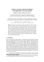
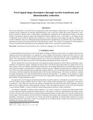
The results are summarized in Figure 2. Both <strong>the</strong> batch VB method and<br />
<strong>the</strong> <strong>on</strong>line VB method gave <strong>the</strong> highest free energy for <strong>the</strong> true model c<strong>on</strong>sisting<br />
of four units. The <strong>on</strong>line VB method with <strong>the</strong> discount factor showed<br />
faster and better performance than <strong>the</strong> batch VB method, especially for large<br />
amounts of data (see Figure 2). The reas<strong>on</strong> for this performance difference<br />
can be c<strong>on</strong>sidered as follows. In <strong>the</strong> <strong>on</strong>line VB method, <strong>the</strong> posterior probability<br />
for hidden variables is calculated by using <strong>the</strong> newly calculated ensemble<br />
average of <strong>the</strong> parameters improved at each observati<strong>on</strong>. The batch<br />
VB method, in c<strong>on</strong>trast, uses <strong>the</strong> ensemble average of <strong>the</strong> parameters calculated<br />
in <strong>the</strong> previous epoch for all data. Therefore, <strong>the</strong> estimati<strong>on</strong> quality of<br />
<strong>the</strong> posterior probability for <strong>the</strong> hidden variables improves ra<strong>the</strong>r slowly.<br />
This becomes more prominent for larger amounts of data. In this case, <strong>the</strong><br />
<strong>on</strong>line VB method can �nd <strong>the</strong> optimal soluti<strong>on</strong> within <strong>on</strong>e epoch, as shown<br />
in Figure 2B.
<str<strong>on</strong>g>Online</str<strong>on</strong>g> <str<strong>on</strong>g>Model</str<strong>on</strong>g> <str<strong>on</strong>g>Selecti<strong>on</strong></str<strong>on</strong>g> <str<strong>on</strong>g>Based</str<strong>on</strong>g> <strong>on</strong> <strong>the</strong> Variati<strong>on</strong>al <strong>Bayes</strong> 1669<br />
Figure 2: Maximum free energies (FE) obtained by three learning methods and<br />
<strong>the</strong>ir c<strong>on</strong>vergence times measured by epoch numbers are plotted for various<br />
models. Three methods are batch VB (dash-dotted line with square), <strong>on</strong>line VB<br />
with discount factor (solid line with circles), and <strong>on</strong>line VB without discount<br />
factor (dashed line with triangles). The abscissa denotes <strong>the</strong> number of gaussian<br />
units in trained models. (A) Results for data set A. (B) Results for data set B.<br />
The <strong>on</strong>line VB method without <strong>the</strong> discount factor showed poor performance<br />
and slow c<strong>on</strong>vergence for all cases. This result implies that <strong>the</strong><br />
introducti<strong>on</strong> of <strong>the</strong> discount factor is crucial for good performance of <strong>the</strong><br />
<strong>on</strong>line VB method, as pointed out in secti<strong>on</strong> 3. If <strong>the</strong>re is no discount factor,<br />
<strong>the</strong> early inaccurate estimati<strong>on</strong>s c<strong>on</strong>tribute to <strong>the</strong> suf�cient statistics average<br />
even in <strong>the</strong> later stages of <strong>the</strong> learning process and degrade <strong>the</strong> quality<br />
of estimati<strong>on</strong>s.<br />
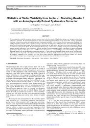
In <strong>the</strong> sec<strong>on</strong>d experiment, <strong>the</strong> sequential model selecti<strong>on</strong> procedure using<br />
a trial model (see secti<strong>on</strong> 4) was tested. When <strong>the</strong> free energy c<strong>on</strong>verged, <strong>the</strong><br />
structure of <strong>the</strong> trial model was changed based <strong>on</strong> <strong>the</strong> base model, which was<br />
<strong>the</strong> best model to date. We tested two initial model c<strong>on</strong>�gurati<strong>on</strong>s c<strong>on</strong>sisting<br />
of 2 units and 10 units. When <strong>the</strong> model structure was changed, <strong>the</strong> discount<br />
factor and <strong>the</strong> effective learning c<strong>on</strong>stant in <strong>the</strong> <strong>on</strong>line VB method were reset<br />
as (1 ¡l(t )) D 0.01 and g(t ) D 0.01. The <strong>on</strong>line VB method was able to �nd<br />
<strong>the</strong> best model in all cases (see Figures 3 and 4). It should be noted that <strong>the</strong><br />
VB method sometimes increased <strong>the</strong> free energy while decreasing <strong>the</strong> data<br />
likelihood (see Figures 3–6). This was achieved as a result of <strong>the</strong> decrease
1670 Masa-aki Sato<br />
Figure 3: <str<strong>on</strong>g>Online</str<strong>on</strong>g> model selecti<strong>on</strong> processes using <strong>the</strong> <strong>on</strong>line VB method for data<br />
set A. Free energies (FE) and number of units for <strong>the</strong> base model (solid line),<br />
which is <strong>the</strong> best model to date, and <strong>the</strong> current trial model (dash-dotted line)<br />
are shown. Log likelihood (LKD) for <strong>the</strong> current trial model (dashed line) is also<br />
shown. (A) The initial model c<strong>on</strong>sists of 2 units. (B) The initial model c<strong>on</strong>sists<br />
of 10 units.<br />
in <strong>the</strong> model complexity. The batch VB method also found <strong>the</strong> best model<br />
(see Figures 5 and 6) except for <strong>on</strong>e case, in which <strong>the</strong> batch VB method got<br />
stuck in a local maximum (see Figure 6A).<br />
We also examined <strong>the</strong> <strong>on</strong>line model selecti<strong>on</strong> procedure for a dynamic envir<strong>on</strong>ment<br />
using a hierarchical mixture of MG models described in secti<strong>on</strong> 4.<br />
The hierarchical mixture in this experiment c<strong>on</strong>sisted of two MG models.<br />
Both models started from <strong>the</strong> same model structure with 10 units. When<br />
<strong>the</strong> free energies c<strong>on</strong>verged, <strong>the</strong> structure of a MG model with lower free<br />
energy was changed. At <strong>the</strong> moment, <strong>the</strong> discount factor and <strong>the</strong> effective<br />
learning c<strong>on</strong>stant were reset as (1 ¡ l(t )) D 0.01 and g(t ) D 0.01.<br />
In this experiment, <strong>the</strong> data generati<strong>on</strong> model was changed at <strong>the</strong> �fty-<br />
�rst epoch. In <strong>the</strong> �rst 50 epochs, <strong>the</strong> number of gaussians was four. After <strong>the</strong>
<str<strong>on</strong>g>Online</str<strong>on</strong>g> <str<strong>on</strong>g>Model</str<strong>on</strong>g> <str<strong>on</strong>g>Selecti<strong>on</strong></str<strong>on</strong>g> <str<strong>on</strong>g>Based</str<strong>on</strong>g> <strong>on</strong> <strong>the</strong> Variati<strong>on</strong>al <strong>Bayes</strong> 1671<br />
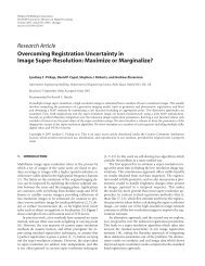
Figure 4: <str<strong>on</strong>g>Online</str<strong>on</strong>g> model selecti<strong>on</strong> processes using <strong>the</strong> <strong>on</strong>line VB method for<br />
data set B. Free energies (FE) and number of units for <strong>the</strong> base model (solid<br />
line), which is <strong>the</strong> best model to date, and <strong>the</strong> current trial model (dash-dotted<br />
line) are shown. Log likelihood (LKD) for <strong>the</strong> current trial model (dashed line)<br />
is also shown. (A) The initial model c<strong>on</strong>sists of 2 units. (B) The initial model<br />
c<strong>on</strong>sists of 10 units.<br />
�fty-�rst epoch, <strong>the</strong> number of gaussians was six. In <strong>the</strong> learning process,<br />
each model observed 1000 data in <strong>on</strong>e epoch. Figure 7 shows <strong>the</strong> learning<br />
process. After <strong>the</strong> twentieth epoch, <strong>the</strong> optimal model structure with four<br />
units was found. When <strong>the</strong> envir<strong>on</strong>ment was changed at <strong>the</strong> �fty-�rst epoch,<br />
<strong>the</strong> free energies of both models dropped dramatically. The trained models<br />
tried to search for <strong>the</strong> new optimal structure. After <strong>the</strong> seventy-�fth epoch,<br />
<strong>the</strong> optimal model structure with six units was found. The result showed<br />
that <strong>the</strong> <strong>on</strong>line VB method was able to adjust <strong>the</strong> model structure to dynamic<br />
envir<strong>on</strong>ment.
1672 Masa-aki Sato<br />
Figure 5: Sequential model selecti<strong>on</strong> processes using <strong>the</strong> batch VB method for<br />
data set A. Free energies (FE) and number of units for <strong>the</strong> base model (solid<br />
line), which is <strong>the</strong> best model to date, and <strong>the</strong> current trial model (dash-dotted<br />
line) are shown. Log likelihood (LKD) for <strong>the</strong> current trial model (dashed line)<br />
is also shown. (A) The initial model c<strong>on</strong>sists of 2 units. (B) The initial model<br />
c<strong>on</strong>sists of 10 units.<br />
6 C<strong>on</strong>clusi<strong>on</strong><br />
We derived an <strong>on</strong>line versi<strong>on</strong> of <strong>the</strong> VB algorithm and proved its c<strong>on</strong>vergence<br />
by showing that it is a stochastic approximati<strong>on</strong> for �nding <strong>the</strong> maximum<br />
of <strong>the</strong> free energy. A fully <strong>on</strong>line learning method with a model selecti<strong>on</strong><br />
mechanism was also proposed based <strong>on</strong> <strong>the</strong> <strong>on</strong>line VB method, toge<strong>the</strong>r<br />
with a sequential model selecti<strong>on</strong> procedure. This method can be applied<br />
to real-time applicati<strong>on</strong>s.<br />
We c<strong>on</strong>sidered <strong>the</strong> <strong>Bayes</strong> model without hierarchy. The current method<br />
can be easily extended to <strong>the</strong> hierarchical <strong>Bayes</strong> model (see appendix D).
<str<strong>on</strong>g>Online</str<strong>on</strong>g> <str<strong>on</strong>g>Model</str<strong>on</strong>g> <str<strong>on</strong>g>Selecti<strong>on</strong></str<strong>on</strong>g> <str<strong>on</strong>g>Based</str<strong>on</strong>g> <strong>on</strong> <strong>the</strong> Variati<strong>on</strong>al <strong>Bayes</strong> 1673<br />
Figure 6: Sequential model selecti<strong>on</strong> processes using <strong>the</strong> batch VB method for<br />
data set B. Free energies (FE) and number of units for <strong>the</strong> base model (solid line),<br />
which is <strong>the</strong> best model to date, and <strong>the</strong> current trial model (dash-dotted line)<br />
are shown. Log likelihood (LKD) for <strong>the</strong> current trial model (dashed line) is also<br />
shown. (A) The initial model c<strong>on</strong>sists of 2 units. (B) The initial model c<strong>on</strong>sists<br />
of 10 units.<br />
In preliminary experiments using syn<strong>the</strong>tic data, <strong>the</strong> <strong>on</strong>line VB method<br />
was able to adapt <strong>the</strong> model structure to dynamic envir<strong>on</strong>ments. A detailed<br />
study <strong>on</strong> <strong>the</strong> performance of <strong>the</strong> <strong>on</strong>line VB method will be published in a<br />
forthcoming article. It also remains for future study to �nd better sequential<br />
model selecti<strong>on</strong> procedure.<br />
Appendix A<br />
Free energy maximizati<strong>on</strong> can be d<strong>on</strong>e by using <strong>the</strong> following <strong>the</strong>orem:
1674 Masa-aki Sato<br />
Figure 7: <str<strong>on</strong>g>Online</str<strong>on</strong>g> model selecti<strong>on</strong> processes for dynamic envir<strong>on</strong>ment using hierarchical<br />
mixture of MG models. The number of units in <strong>the</strong> data generati<strong>on</strong><br />
model is four in <strong>the</strong> �rst 50 epochs and six after <strong>the</strong> �fty-�rst epoch. Free energies<br />
(FE) and number of units for best model (solid line), which is selected at<br />
<strong>the</strong> previous competiti<strong>on</strong>, and trial model (dashed line) are shown.<br />
Theorem 1. The maximum of ( R dm (y)Q(y)( f (y) ¡log(Q(y)))) under <strong>the</strong> c<strong>on</strong>diti<strong>on</strong>,<br />
R dm (y)Q(y) D 1, is given by<br />
Q(y) D<br />
exp[ f (y)]<br />
R dm (y0) exp[ f (y0)] .<br />
The <strong>the</strong>orem can be proved with <strong>the</strong> help of <strong>the</strong> Lagrange multiplier method.<br />
The VB equati<strong>on</strong>s, 2.13 through 2.19, can be proved by using this <strong>the</strong>orem<br />
and <strong>the</strong> following relati<strong>on</strong>s:<br />
Z<br />
F D<br />
dm (µ )Qh (µ )<br />
£ £ T ¡ hr(x, z)iQz ¢ µ ¡ Ã (µ )¢ C log P0(µ ) ¡ log Qh (µ )¤
<str<strong>on</strong>g>Online</str<strong>on</strong>g> <str<strong>on</strong>g>Model</str<strong>on</strong>g> <str<strong>on</strong>g>Selecti<strong>on</strong></str<strong>on</strong>g> <str<strong>on</strong>g>Based</str<strong>on</strong>g> <strong>on</strong> <strong>the</strong> Variati<strong>on</strong>al <strong>Bayes</strong> 1675<br />
C Qh (µ )-independent terms<br />
Z<br />
D dm (ZfTg)Qz(ZfTg)<br />
" TX<br />
#<br />
£ (r(x(t), Z(t)) ¢ hµiQ C r0(x(t), Z(t))) ¡ log Qz(ZfTg)<br />
h<br />
tD1<br />
C Qz(ZfTg) - independent terms,<br />
where h¢iQ and h¢iQz denote <strong>the</strong> expectati<strong>on</strong> value with respect to Q h h (µ ) and<br />
Qz(ZfTg), respectively.<br />
Appendix B<br />
The calculati<strong>on</strong> of <strong>the</strong> derivative of <strong>the</strong> parameterized free energy (see equati<strong>on</strong><br />
2.26) is lengthy but straightforward. The outline of <strong>the</strong> calculati<strong>on</strong> is<br />
shown below. The derivative with respect to µ<br />
N can be calculated as<br />
@F/@ N �<br />
@<br />
µ D T<br />
@N µ hr(x, z)i ´<br />
N (hµi<br />
µ ® ¡ µ N ),<br />
by using <strong>the</strong> relati<strong>on</strong><br />
@<br />
@N �TX ´ �<br />
log P(x(t)| µ<br />
N ) D T hr(x, z)i N ¡<br />
µ<br />
µ @Ã<br />
@N ´<br />
.<br />
µ<br />
tD1<br />
The coef�cient matrix T(@hri N /@<br />
µ N µ ) turns out to be U(µ ) de�ned in equati<strong>on</strong><br />
2.28.<br />
The derivatives with respect to (®, c ) are given by<br />
1<br />
c<br />
@F<br />
@® D<br />
�<br />
1<br />
c 2<br />
@ 2 W<br />
@®@® T<br />
´<br />
¢ ± ²<br />
Thr(x, z)i N C c 0®0 ¡ (T C c 0)®<br />
µ<br />
�<br />
1 @<br />
C (T C c 0 ¡c )<br />
c<br />
2 W 1<br />
¡<br />
@®@c c 2<br />
´<br />
@W<br />
,<br />
@®<br />
1<br />
¡<br />
c 2<br />
´<br />
@W<br />
¢<br />
@®<br />
± ²<br />
Thr(x, z)i N C c 0®0 ¡ (T C c 0)®<br />
µ<br />
� 2 ´<br />
@ W<br />
C (T C c 0 ¡c ) .<br />
@c @c<br />
@F<br />
@c D<br />
�<br />
1 @<br />
c<br />
2 W<br />
@®@c<br />
Equati<strong>on</strong>s 2.30 and 2.31 can be derived by using <strong>the</strong> above and <strong>the</strong> following<br />
equati<strong>on</strong>s:<br />
1<br />
c 2<br />
@ 2 W 1<br />
D<br />
T @®@® c 2<br />
½ � @ log P a<br />
@®<br />
´ �<br />
@ log Pa @® T<br />
´¾<br />
,<br />
®
1676 Masa-aki Sato<br />
1<br />
c<br />
@ 2 W<br />
@®@c<br />
Appendix C<br />
½ � ´ � ´¾<br />
1 @ log Pa @ log Pa D ,<br />
c @® @c ®<br />
@ 2 W<br />
@c @c D<br />
½ � ´ � ´¾<br />
@ log Pa @ log Pa .<br />
@c @c ®<br />
1<br />
¡<br />
c 2<br />
@W<br />
@®<br />
The VB algorithm for <strong>the</strong> mixture of Gaussian model is brie�y explained in<br />
this appendix. (Notati<strong>on</strong>s in this appendix are slightly different from those<br />
in <strong>the</strong> text.) We �rst explain more general mixture models: <strong>the</strong> mixture of<br />
exp<strong>on</strong>ential family (MEF) models. The probability distributi<strong>on</strong> for <strong>the</strong> ith<br />
unit in <strong>the</strong> MEF model is de�ned by<br />
P(x| µi, i) D exp[ri(x) ¢ µi C ri, 0(x) ¡ Yi(µi)]. (C.1)<br />
The c<strong>on</strong>jugate distributi<strong>on</strong> for equati<strong>on</strong> C.1 is given by<br />
P a (µi | ®i, c i, i) D exp[c i(®i ¢ µi ¡ Yi(µi)) ¡ Wi(®i, c i)]. (C.2)<br />
The probability distributi<strong>on</strong> for <strong>the</strong> MEF model is <strong>the</strong>n de�ned by<br />
MX<br />
P(x|g, µ ) D giP(x| µi, i)<br />
iD1<br />
D X<br />
"<br />
MX �<br />
exp zi(log gi ¡ Yi(µi))<br />
fzg iD1<br />
´#<br />
C ziri(x) ¢ µi C ziri,0(x)<br />
, (C.3)<br />
where <strong>the</strong> hidden variable z D fzi |i D 1, . . . , Mg is an indicator variable:<br />
zi D 0 or 1, and PM<br />
iD1 zi D 1. P fzg denotes <strong>the</strong> summati<strong>on</strong> over M possible<br />
c<strong>on</strong>�gurati<strong>on</strong>s of z. The mixing proporti<strong>on</strong> g D fgi |i D 1, . . . , Mg satis�es <strong>the</strong><br />
c<strong>on</strong>straint PM<br />
iD1 gi D 1, which is automatically satis�ed by <strong>the</strong> expressi<strong>on</strong><br />
gi D eQi /( PM<br />
jD1 eQj ).<br />
The set of model parameters fg, µg D fgi, µi |i D 1, . . . , Mg is not <strong>the</strong> natural<br />
parameter of <strong>the</strong> MEF model (see equati<strong>on</strong> C.3). The natural parameter<br />
is given by f!, µg D fvi D Qi ¡ Yi(µi), µi |i D 1, . . . , Mg. The corresp<strong>on</strong>ding<br />
suf�cient statistics is given by fzi, ziri(x)|i D 1, . . . , Mg. Accordingly, <strong>the</strong><br />
MEF model can be written as <strong>the</strong> EFH model:<br />
"<br />
X MX<br />
P(x| !, µ ) D exp<br />
fzg<br />
iD1<br />
¡ ¢<br />
zivi C ziri(x) ¢ µi ¡ Yh (!, µ )<br />
#<br />
, (C.4)
<str<strong>on</strong>g>Online</str<strong>on</strong>g> <str<strong>on</strong>g>Model</str<strong>on</strong>g> <str<strong>on</strong>g>Selecti<strong>on</strong></str<strong>on</strong>g> <str<strong>on</strong>g>Based</str<strong>on</strong>g> <strong>on</strong> <strong>the</strong> Variati<strong>on</strong>al <strong>Bayes</strong> 1677<br />
Yh (!,<br />
"<br />
MX<br />
#<br />
µ ) D log exp(vi C Yi(µi)) . (C.5)<br />
iD1<br />
The c<strong>on</strong>jugate distributi<strong>on</strong> for <strong>the</strong> MEF model, equati<strong>on</strong> C.3, is given by <strong>the</strong><br />
product of <strong>the</strong> Dirichlet distributi<strong>on</strong> and <strong>the</strong> c<strong>on</strong>jugate distributi<strong>on</strong> for each<br />
unit:<br />
P a (g, µ | ®, º, c ) D exp<br />
Wa (®, º, c ) D<br />
D exp<br />
"<br />
"<br />
c<br />
c<br />
MX<br />
¡ ¢<br />
ºi log gi ¡ Yi(µi) C ®i ¢ µi ¡ Wa (®, º, c )<br />
iD1<br />
MX<br />
(ºivi C ºi®i ¢ µi)<br />
iD1<br />
¡c Yh (!, µ ) ¡ Wa(®, º, c )<br />
MX<br />
log C (c ºi C 1)<br />
iD1<br />
¡ log C (c C M) C<br />
#<br />
#<br />
, (C.6)<br />
MX<br />
Wi(®i, c ºi), (C.7)<br />
where ºi satis�es PM<br />
iD1 ºi D 1, and C (c ) is <strong>the</strong> gamma functi<strong>on</strong>, that is,<br />
C (c ) D R 1<br />
0 dse¡s s c ¡1 . The VB algorithm for <strong>the</strong> MEF model can be derived<br />
by using Wa as described in secti<strong>on</strong> 2. The VB E-step equati<strong>on</strong> is given by<br />
Nµi D hµii ® D 1<br />
c ºi<br />
Nvi D hvii ® D 1<br />
c<br />
@Wa<br />
@®i<br />
@Wa<br />
@ºi<br />
The VB M-step equati<strong>on</strong> is given by<br />
iD1<br />
, (C.8)<br />
¡ ®i ¢ hµii ® . (C.9)<br />
c D T C c (0), (C.10)<br />
ºi D 1 ±<br />
Thzii N C c (0)ºi(0)<br />
c µ ² , (C.11)<br />
®i D 1 ±<br />
Thziri(x)i N C c (0)ºi(0)®i(0)<br />
c ºi µ ² , (C.12)<br />
where c (0) and fºi(0), ®i(0)|i D 1, . . . , Mg are <strong>the</strong> prior hyperparameters<br />
of <strong>the</strong> prior parameter distributi<strong>on</strong>. h¢i N µ denotes <strong>the</strong> expectati<strong>on</strong> value (see<br />
equati<strong>on</strong> 2.19) with respect to P(z|x, N!, N µ ).
1678 Masa-aki Sato<br />
The free energy of <strong>the</strong> MEF model after <strong>the</strong> VB M-step is expressed as<br />
F D<br />
MX h<br />
Thzi log P(x| N!, µ N )i N ¡ Thzi log P(x, z| N!, µ N )i N<br />
µ µ<br />
iD1<br />
C log C(c ºi C 1) ¡ºi log C (c C M)<br />
¡ log C(c (0)ºi(0) C 1) C ºi(0) log C (c (0) C M)<br />
C Wi(®i, c ºi) ¡ Wi(®i(0), c (0)ºi(0)) i . (C.13)<br />
The mixture of Gaussian (MG) model is obtained when <strong>the</strong> comp<strong>on</strong>ent<br />
distributi<strong>on</strong> P(x| µi, i) is <strong>the</strong> normal distributi<strong>on</strong>:<br />
P(x|mi, Si, i) D (2p ) ¡N/2 | Si | 1/2 µ<br />
exp ¡ 1<br />
2 (x ¡ mi) T <br />
Si(x ¡ mi)<br />
µ<br />
D exp ¡ 1<br />
2 xT Six C x T <br />
Simi ¡ Yi(mi, Si) , (C.14)<br />
Yi(mi, Si) D 1<br />
2 mT i Simi C 1<br />
2 log | Si | ¡ N<br />
2 log(2p ), (C.15)<br />
where mi and Si denote <strong>the</strong> center and <strong>the</strong> inverse covariance matrix of <strong>the</strong><br />
ith gaussian. The natural parameter of <strong>the</strong> normal distributi<strong>on</strong> is given by<br />
µi D ( Si, Simi). The c<strong>on</strong>jugate distributi<strong>on</strong> for <strong>the</strong> normal distributi<strong>on</strong> (see<br />
equati<strong>on</strong> C.14) is given by <strong>the</strong> normal Wishart distributi<strong>on</strong> (Gelman et al.,<br />
1995),<br />
P a (mi, Si |ci, Di, c i) D exp<br />
"<br />
¡ 1<br />
2 c i(mi ¡ ci) T Si(mi ¡ ci)<br />
¡ 1<br />
¡1<br />
c iTr(SiD i ) C<br />
2 1<br />
2 (c<br />
#<br />
i ¡ N) log | Si | ¡ Wi(Di, c i) , (C.16)<br />
Wi(Di, c i) D 1<br />
2 c i log |D ¡1<br />
i | C<br />
NX<br />
� ´<br />
c i C 1 ¡ n<br />
log C<br />
2<br />
nD1<br />
¡ 1<br />
2 c iN log ± c ²<br />
i N<br />
¡<br />
2 2 log ± c ²<br />
i 1<br />
C<br />
2p 4 N(N ¡ 1) logp. (C.17)<br />
The natural parameter of <strong>the</strong> c<strong>on</strong>jugate distributi<strong>on</strong>, equati<strong>on</strong> C.16, is given<br />
by<br />
(c i®i, c i) D (c i(D ¡1<br />
i C cic T i ), c ici, c i). (C.18)<br />
The VB algorithm for <strong>the</strong> MG model can be derived by using <strong>the</strong> above<br />
equati<strong>on</strong>s.
<str<strong>on</strong>g>Online</str<strong>on</strong>g> <str<strong>on</strong>g>Model</str<strong>on</strong>g> <str<strong>on</strong>g>Selecti<strong>on</strong></str<strong>on</strong>g> <str<strong>on</strong>g>Based</str<strong>on</strong>g> <strong>on</strong> <strong>the</strong> Variati<strong>on</strong>al <strong>Bayes</strong> 1679<br />
Appendix D<br />
The VB method can be easily extended to <strong>the</strong> hierarchical <strong>Bayes</strong> model. Let<br />
us c<strong>on</strong>sider <strong>the</strong> EFH model (see equati<strong>on</strong> 2.1) with <strong>the</strong> prior distributi<strong>on</strong><br />
P a (µ | ®0, c 0). The evidence for <strong>the</strong> hierarchical <strong>Bayes</strong> model is given by <strong>the</strong><br />
marginal likelihood with respect to <strong>the</strong> model parameter µ and <strong>the</strong> prior<br />
hyperparameter ®0,<br />
Z<br />
P(XfTg) D dm (h )dm (®0)P(XfTg| µ )Pa (µ | ®0, c 0)P0(®0), (D.1)<br />
where P0(®0) is <strong>the</strong> prior distributi<strong>on</strong> for <strong>the</strong> prior hyperparameter ®0. The<br />
free energy is de�ned by<br />
Z<br />
F(XfTg, Q) D dm (µ )dm (®0)dm (ZfTg)Q(µ, ®0, ZfTg)<br />
�<br />
P(XfTg, ZfTg| µ )Pa (µ<br />
£ log<br />
| ´<br />
®0, c 0)P0(®0)<br />
. (D.2)<br />
Q(µ, ®0, ZfTg)<br />
The hierarchical VB method can be obtained assuming <strong>the</strong> c<strong>on</strong>jugate prior<br />
for P a (µ | ®0, c 0),<br />
P0(®0) D exp [b0 (a0®0c 0 ¡ Wa (®0, c 0)) ¡ Wa(a0, b0)] , (D.3)<br />
and <strong>the</strong> factorizati<strong>on</strong> for <strong>the</strong> trial posterior distributi<strong>on</strong>,<br />
Q(µ, ®0, ZfTg) D Q h (µ )Q a (®0)Qz(ZfTg). (D.4)<br />
The remaining calculati<strong>on</strong>s can be d<strong>on</strong>e by <strong>the</strong> same way as in <strong>the</strong> VB<br />
method. The VB algorithm in this case c<strong>on</strong>sists of three steps. The posterior<br />
probability for <strong>the</strong> hidden variable P(z(t)|x(t), N µ ) is calculated in <strong>the</strong> VB<br />
E-step by using <strong>the</strong> ensemble average of <strong>the</strong> parameters<br />
N<br />
µ D hµi ® . (D.5)<br />
The posterior hyperparameter ® is calculated in <strong>the</strong> VB M-step,<br />
c ® D Thr(x, z)i N µ C c 0h®0ia, (D.6)<br />
c 0h®0ia D c 0<br />
Z<br />
dm (®0)Q a (®0)®0 D 1<br />
b<br />
@Wa<br />
(a, b), (D.7)<br />
@a<br />
toge<strong>the</strong>r withc D T C c 0. The posterior hyper-hyperparameter (a, b) is <strong>the</strong>n<br />
calculated:<br />
a D hµi ® C a0, (D.8)
1680 Masa-aki Sato<br />
b D b0 C 1, (D.9)<br />
hµi ® D 1<br />
c<br />
@Wa<br />
@® (®, c ). (D.10)<br />
Repeating <strong>the</strong> above three steps, <strong>the</strong> free energy m<strong>on</strong>ot<strong>on</strong>ically increases.<br />
The <strong>on</strong>line VB algorithm can be similarly derived.<br />
References<br />
Amari, S. (1985).Differential geometrical method in statistics. New York: Springer-<br />
Verlag.<br />
Amari, S. (1998). Natural gradient works ef�ciently in learning. Neural Computati<strong>on</strong>,<br />
10, 251–276.<br />
Attias, H. (1999). Inferring parameters and structure of latent variable models<br />
by variati<strong>on</strong>al <strong>Bayes</strong>. In Proc. 15th C<strong>on</strong>ference <strong>on</strong> Uncertainty in Arti�cial<br />
Intelligence (pp. 21–30).<br />
Attias, H. (2000). A variati<strong>on</strong>al <strong>Bayes</strong>ian framework for graphical models. In<br />
S. A. Solla, T. K. Leen, & K.-R. Müller (Eds.), Advances in neural informati<strong>on</strong><br />
processing systems, 12. Cambridge, MA: MIT Press (pp. 206–212).<br />
Bishop, C. M. (1995). Neural networks for pattern recogniti<strong>on</strong>. New York: Oxford<br />
University Press.<br />
Bishop, C. M. (1999). Variati<strong>on</strong>al principal comp<strong>on</strong>ents. In IEE C<strong>on</strong>ference Publicati<strong>on</strong><br />
<strong>on</strong> Arti�cial Neural Networks ICANN99 (pp. 509–514).<br />
Chickering, D. M., & Heckerman, D. (1997). Ef�cient approximati<strong>on</strong>s for <strong>the</strong><br />
marginal likelihood of <strong>Bayes</strong>ian networks with hidden variables. Machine<br />
Learning, 29, 181–212.<br />
Cooper, G., & Herskovitz, E. (1992). A <strong>Bayes</strong>ian method for <strong>the</strong> inducti<strong>on</strong> of<br />
probabilistic networks from data. Machine Learning, 9, 309–347.<br />
Dempster, A. P., Laird, N. M., & Rubin, D. B. (1977). Maximum likelihood from<br />
incomplete data via <strong>the</strong> EM algorithm. Journal of Royal Statistical Society B, 39,<br />
1–22.<br />
Gelman, A., Carlin, J. B., Stern, H. S., & Rubin, D. B. (1995). <strong>Bayes</strong>ian data analysis.<br />
L<strong>on</strong>d<strong>on</strong>: Chapman & Hall.<br />
Ghahramani, Z., & Beal, M. J. (2000). Variati<strong>on</strong>al inference for <strong>Bayes</strong>ian mixture<br />
of factor analysers. In S. A. Solla, T. K. Leen, & K.-R. Müller (Eds.), Advances in<br />
neural informati<strong>on</strong> processing systems, 12. Cambridge, MA: MIT Press (pp. 449–<br />
455).<br />
Heckerman, D., Geiger, D., & Chickering, D. (1995). Learning <strong>Bayes</strong>ian networks:<br />
The combinati<strong>on</strong> of knowledge and statistical data. Machine Learning, 20, 197–<br />
243.<br />
Kushner, H. J., & Yin, G. G. (1997). Stochastic approximati<strong>on</strong> algorithms and applicati<strong>on</strong>s.<br />
New York: Springer-Verlag.<br />
Mackay, D. J. C. (1992a). <strong>Bayes</strong>ian interpolati<strong>on</strong>. Neural Computati<strong>on</strong>, 4, 405–447.<br />
Mackay, D. J. C. (1992b). A practical <strong>Bayes</strong>ian framework for backpropagati<strong>on</strong><br />
networks. Neural Computati<strong>on</strong>, 4, 448–472.
<str<strong>on</strong>g>Online</str<strong>on</strong>g> <str<strong>on</strong>g>Model</str<strong>on</strong>g> <str<strong>on</strong>g>Selecti<strong>on</strong></str<strong>on</strong>g> <str<strong>on</strong>g>Based</str<strong>on</strong>g> <strong>on</strong> <strong>the</strong> Variati<strong>on</strong>al <strong>Bayes</strong> 1681<br />
Mackay, D. J. C. (1999). Comparis<strong>on</strong> of approximate methods for handling hyperparameters.<br />
Neural Computati<strong>on</strong>, 11, 1035–1068.<br />
Metropolis, N., Rosenbluth, A. W., Rosenbluth, M. N., Teller, A. H., & Teller, E.<br />
(1953). Equati<strong>on</strong>s of state calculati<strong>on</strong>s by fast computing machines. Journal of<br />
Chemical Physics, 21, 1087–1092.<br />
Neal, R. M. (1996). <strong>Bayes</strong>ian learning for neural networks. New York: Springer-<br />
Verlag.<br />
Neal, R. M., & Hint<strong>on</strong>, G. E. (1998). A view of <strong>the</strong> EM algorithm that justi�es<br />
incremental, sparse, and o<strong>the</strong>r variants. In M. I. Jordan (Ed.), Learning in<br />
graphical models (pp. 355–368). Norwell, MA: Kluwer.<br />
Rabiner, L. R. (1989). A tutorial <strong>on</strong> hidden Markov models and selected applicati<strong>on</strong>s<br />
in speech recogniti<strong>on</strong>. Proceedings of <strong>the</strong> IEEE, 77, 257–286.<br />
Richards<strong>on</strong>, S., & Green, P. J. (1997). On <strong>Bayes</strong>ian analysis of mixtures with an<br />
unknown number of comp<strong>on</strong>ents. Journal of <strong>the</strong> Royal Statistical Society B, 59,<br />
731–792.<br />
Rissanen, J. (1987). Stochastic complexity. Journal of <strong>the</strong> Royal Statistical Society B,<br />
49, 223–239, 253–265.<br />
Roberts, S. J., Husmeier, D., Rezek, I., & Penny, W. (1998). <strong>Bayes</strong>ian approaches to<br />
gaussian mixture modeling. IEEE Transacti<strong>on</strong>s <strong>on</strong> Pattern Analysis and Machine<br />
Intelligence, 20, 1133–1142.<br />
Roweis, S. T., & Ghahramani, Z. (1999). A unifying review of linear gaussian<br />
models. Neural Computati<strong>on</strong>, 11, 305–345.<br />
Sato, M. (2000). C<strong>on</strong>vergence of <strong>on</strong>-line EM algorithm. In Proc. of 7th Internati<strong>on</strong>al<br />
C<strong>on</strong>ference <strong>on</strong> Neural Informati<strong>on</strong> Processing ICONIP-2000 Vol. 1 (pp. 476–481).<br />
Sato, M., & Ishii, S. (2000). On-line EM algorithm for <strong>the</strong> normalized gaussian<br />
network. Neural Computati<strong>on</strong>, 12, 407–432.<br />
Schwartz, G. (1978). Estimating <strong>the</strong> dimensi<strong>on</strong> of a model. Annals of Statistics, 6,<br />
461–464.<br />
Tipping, M. E., & Bishop, C. M. (1999). Mixtures of probabilistic principal comp<strong>on</strong>ent<br />
analyzers. Neural Computati<strong>on</strong>, 11, 443–482.<br />
Titteringt<strong>on</strong>, D. M., Smith, A. F. M., & Makov, U. E. (1985). Statistical analysis of<br />
�nite mixture distributi<strong>on</strong>s. New York: Wiley.<br />
Ueda, N. (1999). Variati<strong>on</strong>al <strong>Bayes</strong>ian learning with split and merge operati<strong>on</strong>s (Tech.<br />
Rep. No. PRMU99-174, 67-74). Institute of Electr<strong>on</strong>ics, Informati<strong>on</strong>, and Communicati<strong>on</strong>s<br />
Engineers. (in Japanese)<br />
Ueda, N., Nakano, R., Ghahramani, Z., & Hint<strong>on</strong>, G. E. (1999). SMEM algorithm<br />
for mixture models. In M. S. Kearns, S. A. Solla, & D. A. Cohn (Eds.), Advances<br />
in neural informati<strong>on</strong> processing systems, 11 (pp. 599–605). Cambridge, MA: MIT<br />
Press.<br />
Waterhouse, S., Mackay, D., & Robins<strong>on</strong>, T. (1996). <strong>Bayes</strong>ian methods for mixture<br />
of experts. In D. S. Touretzky, M. C. Mozer, & M. E. Hasselmo (Eds.), Advances<br />
in neural informati<strong>on</strong> processing systems, 8 (pp. 351–357). Cambridge, MA: MIT<br />
Press.<br />
Received December 28, 1999; accepted September 27, 2000.