The Fourier Transform and its applications goals: present the Fourier ...
The Fourier Transform and its applications goals: present the Fourier ...
The Fourier Transform and its applications goals: present the Fourier ...

You also want an ePaper? Increase the reach of your titles
YUMPU automatically turns print PDFs into web optimized ePapers that Google loves.
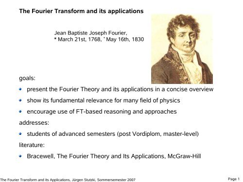
<strong>The</strong> <strong>Fourier</strong> <strong>Transform</strong> <strong>and</strong> <strong>its</strong> <strong>applications</strong><br />
<strong>goals</strong>:<br />
<strong>present</strong> <strong>the</strong> <strong>Fourier</strong> <strong>The</strong>ory <strong>and</strong> <strong>its</strong> <strong>applications</strong> in a concise overview<br />
show <strong>its</strong> fundamental relevance for many field of physics<br />
encourage use of FT-based reasoning <strong>and</strong> approaches<br />
addresses:<br />
students of advanced semesters (post Vordiplom, master-level)<br />
literature:<br />
Jean Baptiste Joseph <strong>Fourier</strong>,<br />
* March 21st, 1768, + May 16th, 1830<br />
Bracewell, <strong>The</strong> <strong>Fourier</strong> <strong>The</strong>ory <strong>and</strong> Its Applications, McGraw-Hill<br />
<strong>The</strong> <strong>Fourier</strong> <strong>Transform</strong> <strong>and</strong> <strong>its</strong> Applications, Jürgen Stutzki, Sommersemester 2007<br />
Page 1
<strong>The</strong> <strong>Fourier</strong> <strong>Transform</strong> <strong>and</strong> <strong>its</strong> <strong>applications</strong><br />
contents:<br />
● ma<strong>the</strong>matical basis<br />
● signal processing: filtering, sampling, reconstruction<br />
● statistics: mean/variance,central limit <strong>the</strong>orem, noise, correlation <strong>and</strong> drift<br />
● optics: diffraction, antenna <strong>the</strong>orem, interferometry<br />
<strong>The</strong> <strong>Fourier</strong> <strong>Transform</strong> <strong>and</strong> <strong>its</strong> Applications, Jürgen Stutzki, Sommersemester 2007<br />
Page 2
<strong>The</strong> <strong>Fourier</strong> <strong>Transform</strong> <strong>and</strong> <strong>its</strong> <strong>applications</strong><br />
contents:<br />
● ma<strong>the</strong>matical basis<br />
– definition, properties, cos-, sine-transform<br />
– convolution, autocorrelation, power spectrum<br />
– often used functions (hat, sinc, ...), δ-function<br />
– FT <strong>the</strong>orems, properties of moments<br />
– periodic functions, <strong>Fourier</strong> series<br />
– discrete <strong>Fourier</strong> transform, FFT<br />
– FT in higher dimensions, cylinder-, spherical coordinates<br />
● signal processing: filtering, sampling, reconstruction<br />
● statistics: mean/variance,central limit <strong>the</strong>orem, noise, correlation <strong>and</strong> drift<br />
● optics: diffraction, antenna <strong>the</strong>orem, interferometry<br />
<strong>The</strong> <strong>Fourier</strong> <strong>Transform</strong> <strong>and</strong> <strong>its</strong> Applications, Jürgen Stutzki, Sommersemester 2007<br />
Page 3
<strong>The</strong> <strong>Fourier</strong> <strong>Transform</strong> <strong>and</strong> <strong>its</strong> <strong>applications</strong><br />
contents:<br />
● ma<strong>the</strong>matical basis<br />
– definition, properties, cos-, sine-transform<br />
– convolution, autocorrelation, power spectrum<br />
– often used functions (hat, sinc, ...), δ-function<br />
– FT <strong>the</strong>orems, properties of moments<br />
– periodic functions, <strong>Fourier</strong> series<br />
– discrete <strong>Fourier</strong> transform, FFT<br />
– FT in higher dimensions, cylinder-, spherical coordinates<br />
● signal processing: filtering, sampling, reconstruction<br />
● statistics: mean/variance,central limit <strong>the</strong>orem, noise, correlation <strong>and</strong> drift<br />
● optics: diffraction, antenna <strong>the</strong>orem, interferometry<br />
<strong>The</strong> <strong>Fourier</strong> <strong>Transform</strong> <strong>and</strong> <strong>its</strong> Applications, Jürgen Stutzki, Sommersemester 2007<br />
Page 4
<strong>The</strong> <strong>Fourier</strong> <strong>Transform</strong> <strong>and</strong> <strong>its</strong> <strong>applications</strong><br />
contents:<br />
● ma<strong>the</strong>matical basis<br />
● signal processing<br />
– filtering<br />
– sampling (Nyquist <strong>the</strong>orem)<br />
– reconstruction<br />
● statistics: mean/variance,central limit <strong>the</strong>orem, noise, correlation <strong>and</strong> drift<br />
● optics: diffraction, antenna <strong>the</strong>orem, interferometry<br />
<strong>The</strong> <strong>Fourier</strong> <strong>Transform</strong> <strong>and</strong> <strong>its</strong> Applications, Jürgen Stutzki, Sommersemester 2007<br />
Page 5
<strong>The</strong> <strong>Fourier</strong> <strong>Transform</strong> <strong>and</strong> <strong>its</strong> <strong>applications</strong><br />
contents:<br />
● ma<strong>the</strong>matical basis<br />
● signal processing: filtering, sampling, reconstruction<br />
● statistics<br />
– mean/variance in time <strong>and</strong> frequency domain,<br />
– Heisenberg relation<br />
– central limit <strong>the</strong>orem<br />
– noise, correlation <strong>and</strong> drift<br />
● optics: diffraction, antenna <strong>the</strong>orem, interferometry<br />
<strong>The</strong> <strong>Fourier</strong> <strong>Transform</strong> <strong>and</strong> <strong>its</strong> Applications, Jürgen Stutzki, Sommersemester 2007<br />
Page 6
<strong>The</strong> <strong>Fourier</strong> <strong>Transform</strong> <strong>and</strong> <strong>its</strong> Applications, Jürgen Stutzki, Sommersemester 2007<br />
drift, natural shapes:<br />
fractional Brownian motion<br />
Page 7
<strong>The</strong> <strong>Fourier</strong> <strong>Transform</strong> <strong>and</strong> <strong>its</strong> <strong>applications</strong><br />
contents:<br />
● ma<strong>the</strong>matical basis<br />
● signal processing: filtering, sampling, reconstruction<br />
● statistics: mean/variance,central limit <strong>the</strong>orem, noise, correlation <strong>and</strong> drift<br />
● optics<br />
– diffraction <strong>the</strong>ory<br />
– antenna <strong>the</strong>orem<br />
– interferometry<br />
<strong>The</strong> <strong>Fourier</strong> <strong>Transform</strong> <strong>and</strong> <strong>its</strong> Applications, Jürgen Stutzki, Sommersemester 2007<br />
Page 8
diffraction image of<br />
circular aperture<br />
interferometry:<br />
left: baseline-tracks of telescope array with earth rotation<br />
right: point-spread-function<br />
<strong>The</strong> <strong>Fourier</strong> <strong>Transform</strong> <strong>and</strong> <strong>its</strong> Applications, Jürgen Stutzki, Sommersemester 2007 Page 9
1. Ma<strong>the</strong>matical Basics<br />
Note: no rigorous proofs here, ra<strong>the</strong>r a “pragmatic” approach<br />
1.1. Definition of <strong>the</strong> <strong>Fourier</strong> <strong>Transform</strong> (FT)<br />
Function f �x�<br />
<strong>Fourier</strong> <strong>Transform</strong> F �s�=∫ −∞<br />
<strong>The</strong> <strong>Fourier</strong> <strong>Transform</strong> <strong>and</strong> <strong>its</strong> Applications, Jürgen Stutzki, Sommersemester 2007<br />
∞<br />
f �x� e −2� i xs dx (“ minus-i ” transform)<br />
note on notation: function f lower capital; <strong>Fourier</strong> transform F upper capital<br />
spatial: x �� s f � x� �� F �s�<br />
time: t �� � f �t � �� F ���<br />
Backtransform, inverse <strong>Fourier</strong> <strong>Transform</strong><br />
Interpretation:<br />
∞<br />
f �x �=∫ F �s� e<br />
−∞<br />
2� i xs ds (“ plus-i “-transform) (prove given below)<br />
<strong>Fourier</strong> <strong>Transform</strong>: filters out <strong>the</strong> (complex) amplitude F �s�=∣F �s�∣e i � s of<br />
e −2� i xs -component, i..e. oscillation with frequency s<br />
Back-<strong>Transform</strong>: express f �x � as sum over e 2�i xs -oscillations with (complex) amplitudes,<br />
i.e. amplitudes <strong>and</strong> phase F �s�=∣F �s�∣e i � s<br />
1<br />
math_ground_1.odt<br />
Page 10
Remark: usual abbreviation: �=2�� (time: angular frequency) or<br />
gives FT:<br />
<strong>and</strong> back-Trafo f �t � = ∫ −∞<br />
k =2�s (spatial: wavenumber)<br />
F� �<br />
��� =F �<br />
2� �= ∞<br />
∫ −∞<br />
�<br />
−2� i<br />
2�<br />
f �t � e t<br />
∞<br />
dt = ∫<br />
−∞<br />
<strong>The</strong> <strong>Fourier</strong> <strong>Transform</strong> <strong>and</strong> <strong>its</strong> Applications, Jürgen Stutzki, Sommersemester 2007<br />
∞<br />
∞<br />
F ��� e 2�i �t d �=∫ −∞<br />
F � �<br />
2� � ei� t d �<br />
2�<br />
f �t� e −i �t dt<br />
1<br />
=<br />
2� ∫ ∞<br />
−∞<br />
�F ��� e i �t d �<br />
2<br />
math_ground_1a.odt<br />
Page 11
or, for symmetry, define: �F ���= 1<br />
� 2� ∫ ∞<br />
−∞<br />
f �t � e −i�t dt <strong>and</strong> back-transform f �t�= 1<br />
�2� ∫ ∞<br />
−∞<br />
<strong>The</strong> <strong>Fourier</strong> <strong>Transform</strong> <strong>and</strong> <strong>its</strong> Applications, Jürgen Stutzki, Sommersemester 2007<br />
�F ��� e i�t d � .<br />
All 1 , 2 , <strong>and</strong> 3<br />
are common notations, used in different fields <strong>and</strong> contexts; we prefer <strong>the</strong> first one.<br />
O<strong>the</strong>r notations often used:<br />
● instead of F �s� : �f �s� or � f �s� .<br />
This is useful to note down certain relations, e.g.� f ⋅g= � f ∗�g (FT of convolution, see below)<br />
● F �s� = FT � f � x �� , operator FT generates <strong>Fourier</strong>-Trafo of function f �x �<br />
3<br />
math_ground_2.odt<br />
Page 12
1.2. Existence of <strong>the</strong> FT<br />
intuitively, <strong>and</strong> from physical insight: each time series has spectrum,<br />
i.e. contains a distribution of frequencies<br />
this applies to all functional dependencies occurring in <strong>the</strong> real world physics<br />
but: even simple examples (which don't as such occur in <strong>the</strong> real world) show problems<br />
● Sine,Cosine: a 0 sin �2��t � , a 0 cos�2�� t� s (needs to be switched on <strong>and</strong> off!)<br />
●<br />
0,<br />
Heavyside Step-Function: H �t �={ 1,<br />
t�0<br />
t�0<br />
●<br />
0,<br />
delta-Funktion, Impuls-Fkt.: � �t �={ ∞ ,<br />
t≠0<br />
t=0 (more specifically �∞<br />
∫ −∞<br />
do not have FT in <strong>the</strong> proper sense<br />
<strong>The</strong> <strong>Fourier</strong> <strong>Transform</strong> <strong>and</strong> <strong>its</strong> Applications, Jürgen Stutzki, Sommersemester 2007<br />
(needs to be switched off!)<br />
��t� dt=1 )<br />
(never gets infinitely sharp!)<br />
<strong>Fourier</strong> transform in <strong>the</strong> proper sense<br />
<strong>the</strong> <strong>Fourier</strong>-<strong>Transform</strong> exists (i.e. <strong>the</strong> <strong>Fourier</strong>-Integral converges for all values of s) if:<br />
∞<br />
1. ∣ f � x �∣ is integrable, i.e. ∫ ∣ f � x�∣ dx exists<br />
−∞<br />
2. f �x � has only finite discontinuities<br />
3. <strong>and</strong> f �x � shows “limited variations” (Lipshitz-Bedingung)<br />
math_ground_3.odt<br />
Page 13
improper <strong>Fourier</strong> <strong>Transform</strong><br />
Many functions allow FT only in <strong>the</strong> “improper” sense: FT in <strong>the</strong> limit:<br />
∞<br />
if ∫ −∞<br />
∞<br />
if ∫ −∞<br />
−� x2<br />
∣f � x�∣ dx does not exist, one considers a modified function f �� x�=e<br />
−� x2<br />
∣e<br />
note: lim<br />
��0<br />
<strong>and</strong> name lim<br />
��0<br />
f ��x�= f � x � ; �≪1 : slowly switching f �x � on <strong>and</strong> off<br />
f � x�∣ dx exists, consider <strong>the</strong> series of varying � , � �0<br />
<strong>The</strong> <strong>Fourier</strong> <strong>Transform</strong> <strong>and</strong> <strong>its</strong> Applications, Jürgen Stutzki, Sommersemester 2007<br />
∞<br />
F ��s�=∫ −∞<br />
e −2� i xs 2<br />
−� x<br />
e<br />
f � x � dx<br />
F ��s�=F �s� <strong>the</strong> (improper) <strong>Fourier</strong> <strong>Transform</strong><br />
Note: such improper FTs are not really functions, but distributions (see below).<br />
f � x� .<br />
math_ground_4.odt<br />
Page 14
1.3 properties of <strong>the</strong> FT<br />
1.3.0 linearity<br />
with h � x �=a f � x ��b g � x � , we get H �s�=a F �s��b G �s�<br />
(proof: linearity of integration)<br />
1.3.1 symmetries<br />
e.g. f �x � real valued, i.e. f * �x �= f �x � , <strong>and</strong> with <strong>the</strong> FT F �s�=∫ e −2� ixs f �x� dx<br />
we get: F * �s� =∫e 2� i xs f * −2� i x �−s�<br />
� x � dx=∫e f � x� dx= F �−s� ,i.e. F �s� is hermitean.<br />
or, more specifically, separating F �s� into real <strong>and</strong> imaginary part:<br />
F �s� = ℜ F �s��i ℑ F �s�<br />
F * �s� = ℜ F �s�−i ℑ F �s�<br />
F �−s� = ℜ F �−s��i ℑ F �−s�<br />
<strong>and</strong> hence<br />
ℜ F �s�=ℜ F �−s� , i.e. ℜ F �s� is even<br />
ℑ F �s�=−ℑ F �−s � , i.e. ℑ F �s� is odd; q.e.d.<br />
Thus: f �x � real valued ⇔ F �s� hermitean<br />
<strong>and</strong> vice versa: f �x � hermitean ⇔ F �s� real valued<br />
Similarly: f �x � imaginary, i.e. f * � x �=− f �x � :<br />
we get F * �s� =∫ e 2� i xs f * � x� dx=−∫ e −2� i x �− s� f �x� dx= −F �−s� ,<br />
Thus: f �x � imaginary ⇔ F �s� anti-hermitean<br />
<strong>and</strong> vice versa f �x � anti-hermitean ⇔ F �s� imaginary<br />
<strong>The</strong> <strong>Fourier</strong> <strong>Transform</strong> <strong>and</strong> <strong>its</strong> Applications, Jürgen Stutzki, Sommersemester 2007<br />
math_ground_5.odt<br />
Page 15
<strong>and</strong> last: f �x � even, i.e. f �x�= f �−x� :<br />
we get<br />
F �s�=∫ e<br />
−∞<br />
−2� i x s f � x� d x =<br />
�<br />
<strong>The</strong> <strong>Fourier</strong> <strong>Transform</strong> <strong>and</strong> <strong>its</strong> Applications, Jürgen Stutzki, Sommersemester 2007<br />
�∞<br />
�∞<br />
=∫ e<br />
−∞<br />
−2� i u�−s � Thus:<br />
f �u� du=F �−s�<br />
f �x � even ⇔ F �s� even<br />
<strong>and</strong> vice versa f �x � odd ⇔ F �s� odd<br />
−∞ �∞<br />
�∞|<br />
u=−x |−∞ ;du=−dx<br />
−∞<br />
−∫ e<br />
�∞<br />
2� i us f �u� d u<br />
,<br />
math_ground_6.odt<br />
Page 16
Note:<br />
any function f �x � can be separated into <strong>its</strong> odd <strong>and</strong> even parts, o � x� <strong>and</strong> e � x � :<br />
with e � x �=e �−x � , o � x�=−o�−x � we have:<br />
f � x� = e� x ��o �x �<br />
f �−x� = e� x �−o �x �<br />
<strong>The</strong> <strong>Fourier</strong> <strong>Transform</strong> <strong>and</strong> <strong>its</strong> Applications, Jürgen Stutzki, Sommersemester 2007<br />
, <strong>and</strong> hence e �x � = 1<br />
2<br />
similarly: separation into real <strong>and</strong> imaginary part:<br />
f �x� = ℜ f � x��i ℑ f � x�<br />
f * �x� = ℜ f � x�−i ℑ f � x�<br />
o � x � = 1<br />
2<br />
� f �x �� f �−x��<br />
.<br />
� f �x �− f �−x��<br />
, <strong>and</strong> ℜ f � x� = 1<br />
2 � f � x�� f * � x��<br />
ℑ f � x� = 1<br />
2i � f � x�− f * � x��<br />
With this, we can separate <strong>the</strong> hermitean <strong>and</strong> anti-hermitean parts:<br />
so that<br />
f �x �=e � x ��o� x �=ℜe � x��i ℑ e � x ��ℜ o� x ��i ℑo � x �<br />
=[ ℜe � x ��i ℑo � x �]<br />
hermitean<br />
anti−hermitean<br />
�[ ℜo �x ��i ℑ e � x� ]<br />
=h� x ��a � x �<br />
f * �−x �= =[ ℜe � x �−�−�i ℑ o �x �]�[−ℜ o� x �−i ℑ e �x �]=h � x �−a �x �<br />
h� x� = 1<br />
2 � f � x�� f * �−x��<br />
a� x� = 1<br />
2 � f � x�− f * �−x��<br />
math_ground_7.odt<br />
Page 17
to summarize:<br />
Symmetry properties of FT<br />
or<br />
f �x � = e � x � � o� x � = ℜ f � x � � i ℑ f �x � = h � x � � a � x �<br />
�<br />
�<br />
�<br />
�<br />
<strong>The</strong> <strong>Fourier</strong> <strong>Transform</strong> <strong>and</strong> <strong>its</strong> Applications, Jürgen Stutzki, Sommersemester 2007<br />
�<br />
�<br />
�<br />
�<br />
F �s� = E �S � � O �s� = H �s� � A �s� = ℜ F �s� � i ℑ F �s�<br />
proof: e.g.<br />
f �x � = ℜe � x � � i ℑ e � x � � ℜ o� x � � i ℑo � x �<br />
�<br />
�<br />
�<br />
�<br />
�<br />
�<br />
F �s� = ℜ E �s� � i ℑ E �s� � i ℑO �S � � ℜO�s�<br />
FT �e� x��= � e� x�= 1�<br />
1<br />
� f �x�� f �−x��=<br />
2<br />
2 ��f � x���f �−x��<br />
= 1<br />
�∞<br />
2 [∫ e<br />
−∞<br />
−2�i xs �∞<br />
f � x� dx�∫ e<br />
−∞<br />
−2� i xs ] f �−x� dx<br />
= 1 [ 2 F �S ��∫<br />
�∞<br />
e<br />
−∞<br />
−2� i u�−s� u] f �u� d<br />
= 1 [ F �s��F �−s�]=E �s�<br />
2<br />
�<br />
�<br />
�<br />
�<br />
� �<br />
�<br />
�<br />
q.e.d.<br />
�<br />
�<br />
math_ground_8.odt<br />
Page 18
1.3.2 FT of <strong>the</strong> complex conjugate function<br />
for <strong>the</strong> <strong>Fourier</strong> <strong>Transform</strong> of f * � x � we get:<br />
FT � f * � x ��= � f * �x �=∫e −2�i xs f * �x � dx<br />
−2� i x �−s<br />
=∫<br />
�]<br />
*<br />
[e f * � x � dx=F * �−s�<br />
with this, <strong>and</strong> with FT � f �−x ��=F �−s� , we can derive all <strong>the</strong> above symmetry relations:<br />
e.g.<br />
FT � ℜ f � x ��=FT� 1<br />
2 [ f � x �� f * 1<br />
� x �]� =<br />
2 [ F �S ��F * �−s�]=H �s� ,<br />
or<br />
etc.<br />
FT �a� x��=FT � 1<br />
2 [ f � x�− f * �−x�]� =1<br />
2 [ F �S�− F* �s�]=i ℑ F �s�<br />
Thus, all symmetry relations above can be derived from <strong>the</strong> (easy to memorize) three<br />
relations:<br />
1) FT � f � x ��=F �s�<br />
2) FT � f �−x ��=F �−s�<br />
3) FT � f * � x ��=F * �−s�<br />
<strong>The</strong> <strong>Fourier</strong> <strong>Transform</strong> <strong>and</strong> <strong>its</strong> Applications, Jürgen Stutzki, Sommersemester 2007<br />
math_ground_9.odt<br />
Page 19
1.4 Sine- <strong>and</strong> Cosine-<strong>Transform</strong>ation<br />
Recall Euler's relation: e i � =cos ��i sin � . Inserting this into <strong>the</strong> definition of <strong>the</strong> FT, we get:<br />
�∞<br />
F �s�=FT � f �x��=∫ e<br />
−∞<br />
−2� i xs f �x� dx=∫ cos�2� xs� f � x � dx – i ∫ sin�2� xs� f �x� dx<br />
−∞<br />
−∞<br />
∞<br />
=∫ 0<br />
f � x�cos�2� xs� dx�∫ −∞<br />
<strong>The</strong> <strong>Fourier</strong> <strong>Transform</strong> <strong>and</strong> <strong>its</strong> Applications, Jürgen Stutzki, Sommersemester 2007<br />
0<br />
�∞<br />
f � x�cos�2� x s� d x<br />
∞<br />
−i∫<br />
0<br />
f � x�sin�2� xs� dx−i ∫<br />
−∞<br />
f � x�sin�2� x s� d x<br />
Substituting in <strong>the</strong> second <strong>and</strong> forth expression:<br />
0 0<br />
| x �−u|∞ ; dx �−du , we get:<br />
∞<br />
=∫ 0<br />
∞<br />
=∫ 0<br />
f � x�cos�2� xs� dx�∫ 0<br />
∞<br />
−∞<br />
f �−u�cos�2�u s� d u<br />
∞<br />
−i∫ 0<br />
[ f � x�� f �−x�] cos�2� xs� dx−i∫ 0<br />
∞<br />
=2∫ 0<br />
e� x� cos�2� xs� dx −i 2∫ 0<br />
∞<br />
�∞<br />
f � x�sin�2� xs� dx� i∫ 0<br />
∞<br />
[ f �x�− f �−x�]sin�2� xs� dx<br />
o� x� sin�2� xs� dx<br />
We define: Cosine-<strong>Transform</strong>ation CT � f � x ��=2∫ 0<br />
Sine-<strong>Transform</strong>ation<br />
∞<br />
∞<br />
0<br />
∞<br />
f �−u�sin�2�u s� d u<br />
f � x � cos�2� xs� dx , <strong>and</strong><br />
ST � f � x��=2∫ f � x� sin�2� xs� dx<br />
0<br />
note: only x�0 counts in CT <strong>and</strong> ST !<br />
math_ground_10.odt<br />
Page 20
F �s�=FT � f � x ��=CT �e �x �� – i ST �o �x ��<br />
i.e. <strong>Fourier</strong> <strong>Transform</strong> ⇔<br />
Cosine-<strong>Transform</strong> of <strong>the</strong> even <strong>and</strong> Sine-<strong>Transform</strong> of <strong>the</strong> odd part of f �x �<br />
Note: as e � x � <strong>and</strong> o � x� need to be defined only for x�0 , <strong>the</strong> continuation to x�0 being<br />
given by symmetry ( e �−x �=e � x � ; o �−x �=−o� x � ), <strong>the</strong> <strong>Fourier</strong> transform carries <strong>the</strong><br />
full information on f �x � , both for x�0 <strong>and</strong> x�0 , although <strong>the</strong> integration in <strong>the</strong> CT<br />
<strong>and</strong> ST only use e � x � <strong>and</strong> o � x� for x�0 .<br />
We can thus, like always, get f �x � back from F �s� through <strong>the</strong> "+i" transform, giving:<br />
f �x�=FT �i � F �s��=CT � E �s���i ST �O�s��<br />
i.e. <strong>Fourier</strong> Backtransform ⇔<br />
Cosine-<strong>Transform</strong> of <strong>the</strong> even <strong>and</strong> Sine-<strong>Transform</strong> of <strong>the</strong> odd part of F �s�<br />
Note: in <strong>the</strong> CT , ST -world (no FT known),<br />
given F �s� , calculate E �s� <strong>and</strong> O�s� , from this, throughCT resp. ST , calculate<br />
f �x �<br />
Symmetries of Cosine- <strong>and</strong> Sine-<strong>Transform</strong>: with F C �s�=CT � f �x �� , F S �s�=ST � f �x�� ,<br />
we have: F C �−s�=F C �s� Cosine-<strong>Transform</strong> is even in s,<br />
F S �−s�=−F S � s� Sine-<strong>Transform</strong> is odd in s<br />
<strong>The</strong> <strong>Fourier</strong> <strong>Transform</strong> <strong>and</strong> <strong>its</strong> Applications, Jürgen Stutzki, Sommersemester 2007<br />
math_ground_11.odt<br />
Page 21
● only <strong>the</strong> behaviour of f �x� for x�0 enters into to Cosine- <strong>and</strong> Sine-<strong>Transform</strong><br />
● <strong>the</strong> symmetries of F C �s� <strong>and</strong> F S �s� imply that <strong>the</strong>y are fully determined by <strong>the</strong>ir s�0<br />
behavior<br />
Thus, only <strong>the</strong> x�0 behavior of an arbitrary function f �x � determines <strong>its</strong> F C �s� <strong>and</strong> F S �s�<br />
Consider a new function f H � x � :<br />
f � x � , x �0<br />
f H � x �={<br />
= f � x� H �x � ,<br />
0, x �0<br />
obtained by "cutting-off" <strong>the</strong> negative<br />
part of f �x � , i.e. by multiplying f �x � with <strong>the</strong> Heavyside step-function defined above.<br />
Obviously, it has <strong>the</strong> same Cosine- <strong>and</strong> Sine transform as f �x � <strong>its</strong>elf:<br />
F S , H �s�=ST � f H � x ��=2∫ 0<br />
∞<br />
=2∫ 0<br />
<strong>and</strong> similarly F C , H �s�=F C �s� .<br />
<strong>The</strong> <strong>Fourier</strong> <strong>Transform</strong> <strong>and</strong> <strong>its</strong> Applications, Jürgen Stutzki, Sommersemester 2007<br />
∞<br />
f H �x � sin �2� xs� dx<br />
f � x � sin �2� xs� dx=ST � f � x ��=F S �s�<br />
Now, e H � x�= 1<br />
2<br />
2 [ f H �x�� f H �−x�]={1<br />
<strong>and</strong> oH �x�= 1<br />
2<br />
2 [ f H � x�− f H �−x�]={1<br />
1<br />
2<br />
− 1<br />
2<br />
f � x� , x�0<br />
f �−x� , x�0<br />
f � x� , x�0<br />
f �−x� , x�0<br />
math_ground_12.odt<br />
Page 22
FT � f � x � H � x ��=CT �e H �x ��−i ST �o H � x ��<br />
= 1<br />
2 [CT � f � x��−i ST � f � x�� ] .<br />
Backtransform of Cosine- <strong>and</strong> Sine-transform<br />
With this, we now consider an arbitrary function f �x � , defined only at x�0 <strong>and</strong> with<br />
CT � f � x ��=F C �s�<br />
ST � f � x��=F S �s�<br />
Note that F C �s� <strong>and</strong> F S �s� , given <strong>the</strong>ir symmetry, have to be taken into account only at<br />
positive frequencies s�0 .<br />
We claim that<br />
<strong>the</strong> back-transform of <strong>the</strong> Cosine transform is <strong>the</strong> Cosine transform:<br />
f � x �=2∫ F C�s� cos �2� xs� ds<br />
0<br />
<strong>and</strong> <strong>the</strong> back-transform of <strong>the</strong> Sine transform is <strong>the</strong> Sine transform:<br />
<strong>The</strong> <strong>Fourier</strong> <strong>Transform</strong> <strong>and</strong> <strong>its</strong> Applications, Jürgen Stutzki, Sommersemester 2007<br />
∞<br />
∞<br />
f � x �=2∫ 0<br />
F S �s� sin�2 � xs� ds<br />
math_ground_13.odt<br />
Page 23
Proof:<br />
1) for <strong>the</strong> Cosine back-trafo:<br />
define an even function for all x : f 1� x �= f �∣x∣�={<br />
Its FT is<br />
FT � f 1 � x ��=F 1 �s�=CT �e 1 � x��<br />
� CT� f 1� x��<br />
−i ST � �o1 �x ��=CT<br />
� f � x��=F C �s�<br />
,<br />
=0<br />
which is also even, being a pure cosine transform:<br />
F 1 �−s�=F 1 �s� , resp. E 1 �s�=F 1 �s � , O 1 �s�=0<br />
Its back-transform reproduces f 1 � x � :<br />
f 1� x �=FT �i � F 1 �s��=CT � E 1�s��<br />
� CT� F 1 �s��<br />
�i ST �O 1 �s��<br />
� =0<br />
� �<br />
=0<br />
ST�F 2 �s��<br />
<strong>The</strong> <strong>Fourier</strong> <strong>Transform</strong> <strong>and</strong> <strong>its</strong> Applications, Jürgen Stutzki, Sommersemester 2007<br />
f � x � , x�0<br />
f �−x � , x�0 , i.e. e 1 � x �= f 1 � x� , o 1 �x �=0 .<br />
=CT �CT � f �∣x∣���<br />
<strong>and</strong> for<br />
x�0 , where f �x � is defined: f � x �= f 1 � x �=CT �CT � f � x �� �=CT � F C � s� � q.e.d.<br />
2) similarly for <strong>the</strong> Sine backtrafo, but with <strong>the</strong> odd function f 2 �x �={ f � x � , x�0<br />
− f �−x � , x�0 :<br />
FT � f 2� x��=F 2�s�=CT � �e 2� x��<br />
=0<br />
−i ST ��o 2� x ��<br />
ST � f 2�x�� =−i ST � f �x ��=−i F S�s� , <strong>and</strong><br />
f 2�x�=FT �i � F 2�s��=CT � E2�s�� �i ST �O 2�s�� =i �−i�ST � F s�s��=ST �ST � f �∣x∣�� �<br />
q.e.d.<br />
Page 24
<strong>The</strong> <strong>Fourier</strong> <strong>Transform</strong> <strong>and</strong> <strong>its</strong> Applications, Jürgen Stutzki, Sommersemester 2007<br />
pltfour.py<br />
Page 25
Summary:<br />
<strong>The</strong> <strong>Fourier</strong> <strong>Transform</strong> <strong>and</strong> <strong>its</strong> Applications, Jürgen Stutzki, Sommersemester 2007<br />
∞<br />
● <strong>Fourier</strong>-<strong>Transform</strong> F �s�=∫ f �x� e<br />
−∞<br />
−2� i xs ●<br />
dx (“ minus-i ” transform)<br />
∞<br />
<strong>Fourier</strong>-Backtransform f �x �=∫ F �s� e<br />
−∞<br />
2� i xs ●<br />
ds (“ plus-i “-transform)<br />
symmetry relations:<br />
f �x � = e � x � � o� x � = ℜ f � x � � i ℑ f �x � = h � x � � a � x �<br />
�<br />
�<br />
�<br />
�<br />
�<br />
�<br />
�<br />
�<br />
F �s� = E �S � � O �s� = H �s� � A �s� = ℜ F �s� � i ℑ F �s�<br />
f �x � = ℜe � x � � i ℑ e � x � � ℜ o� x � � i ℑo � x �<br />
● Cosine-, <strong>and</strong> Sine-<strong>Transform</strong><br />
�<br />
�<br />
�<br />
�<br />
�<br />
�<br />
F �s� = ℜ E �s� � i ℑ E �s� � i ℑO �S � � ℜO�s�<br />
∞<br />
CT � f � x ��=2∫ 0<br />
∞<br />
�<br />
�<br />
f � x � cos�2� xs� dx<br />
ST � f � x ��=2∫ f � x� sin�2� xs� dx<br />
0<br />
which are <strong>the</strong>ir own back-transforms<br />
● <strong>Fourier</strong> <strong>Transform</strong> ⇔<br />
Cosine-<strong>Transform</strong> of <strong>the</strong> even <strong>and</strong> Sine-<strong>Transform</strong> of <strong>the</strong> odd part of f �x �<br />
F �s�=FT � f � x ��=CT �e �x �� – i ST �o �x ��<br />
�<br />
�<br />
� �<br />
�<br />
�<br />
�<br />
�<br />
math_ground_15.odt<br />
Page 26