Image restoration by sparse 3D transform-domain ... - CiteSeerX
Image restoration by sparse 3D transform-domain ... - CiteSeerX
Image restoration by sparse 3D transform-domain ... - CiteSeerX

You also want an ePaper? Increase the reach of your titles
YUMPU automatically turns print PDFs into web optimized ePapers that Google loves.
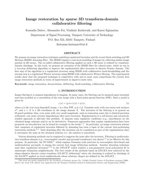
<strong>Image</strong> <strong>restoration</strong> <strong>by</strong> <strong>sparse</strong> <strong>3D</strong> <strong>transform</strong>-<strong>domain</strong><br />
collaborative filtering<br />
Kostadin Dabov, Alessandro Foi, Vladimir Katkovnik, and Karen Egiazarian<br />
Department of Signal Processing, Tampere University of Technology<br />
P.O. Box 553, 33101 Tampere, Finland<br />
firstname.lastname@tut.fi<br />
ABSTRACT<br />
We propose an image <strong>restoration</strong> technique exploiting regularized inversion and the recent block-matching and <strong>3D</strong><br />
filtering (BM<strong>3D</strong>) denoising filter. The BM<strong>3D</strong> employs a non-local modeling of images <strong>by</strong> collecting similar image<br />
patches in <strong>3D</strong> arrays. The so-called collaborative filtering applied on such a <strong>3D</strong> array is realized <strong>by</strong> <strong>transform</strong><strong>domain</strong><br />
shrinkage. In this work, we propose an extension of the BM<strong>3D</strong> filter for colored noise, which we use in<br />
a two-step deblurring algorithm to improve the regularization after inversion in discrete Fourier <strong>domain</strong>. The<br />
first step of the algorithm is a regularized inversion using BM<strong>3D</strong> with collaborative hard-thresholding and the<br />
seconds step is a regularized Wiener inversion using BM<strong>3D</strong> with collaborative Wiener filtering. The experimental<br />
results show that the proposed technique is competitive with and in most cases outperforms the current best<br />
image <strong>restoration</strong> methods in terms of improvement in signal-to-noise ratio.<br />
Keywords: image <strong>restoration</strong>, deconvolution, deblurring, block-matching, collaborative filtering<br />
1. INTRODUCTION<br />
<strong>Image</strong> blurring is a common degradation in imaging. In many cases, the blurring can be assumed space-invariant<br />
and thus modeled as a convolution of the true image with a fixed point-spread function (PSF). Such a model is<br />
given <strong>by</strong><br />
� (�) =(� ~ �)(�)+� (�) , (1)<br />
where � is the true (non-degraded) image, � is a blur PSF, � is i.i.d. Gaussian noise with zero mean and variance<br />
� 2 ,and� � � is a 2D coordinate in the image <strong>domain</strong> �. The inversion of the blurring is in general an<br />
ill-posed problem; thus, even noise with very small magnitude, such as truncation noise due to limited-precision<br />
arithmetic, can cause extreme degradations after naive inversion. Regularization is a well known and extensively<br />
studied approach to alleviate this problem. It imposes some regularity conditions (e.g., smoothness) on the<br />
obtained image estimate and/or on its derivatives. Numerous approaches that employ regularization have been<br />
proposed; an introduction can be found for example in the books. 1, 2 In particular, an image <strong>restoration</strong> scheme<br />
that comprises of regularized inversion followed <strong>by</strong> denoising has been a basis of the current best-performing<br />
<strong>restoration</strong> methods. 3, 4 Such denoising after the inversion can be considered as part of the regularization since<br />
it attenuates the noise in the obtained solution (i.e. the solution is smoothed).<br />
Various denoising methods can be employed to suppress the noise after the inversion. Filtering in multiresolution<br />
<strong>transform</strong> <strong>domain</strong> (e.g., overcomplete wavelet and pyramid <strong>transform</strong>s) was shown 4—6 to be e�ective for this<br />
purpose. In particular, the SV-GSM, 4 which employs Gaussian scale mixtures in overcomplete directional and<br />
multiresolution pyramids, is among the current best image deblurring methods. Another denoising technique<br />
used after regularized inversion 3, 7, 8 is the LPA-ICI 9 which exploits a non-parametric local polynomial fit in<br />
anisotropic estimation neighborhoods. The best results of the methods based on LPA-ICI were achieved <strong>by</strong> the<br />
shape-adaptive discrete cosine <strong>transform</strong> (SA-DCT) deblurring 3 where the denoising is realized <strong>by</strong> shrinkage of<br />
the SA-DCT applied on local neighborhoods whose arbitrary shapes are defined <strong>by</strong> the LPA-ICI.<br />
This work was partly supported <strong>by</strong> the Academy of Finland, project No. 213462 (Finnish Centre of Excellence program [2006 -<br />
2011]); the work of K. Dabov was supported <strong>by</strong> the Tampere Graduate School in Information Science and Engineering (TISE).
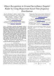
Figure 1. Flowchart of the proposed deconvolution algorithm. A fragment of House illustrates the images after each<br />
operation.<br />
In this work we follow the above <strong>restoration</strong> scheme (regularized inversion followed <strong>by</strong> denoising) exploiting<br />
an extension of the block-matching and <strong>3D</strong> filtering 10 (BM<strong>3D</strong>). This filter is based on the assumption that there<br />
exist mutually similar patches within a natural image – the same assumption used in other non-local image filters<br />
such as. 11, 12 The BM<strong>3D</strong> processes a noisy image in a sliding-window (block) manner, where block-matching is<br />
performed to find blocks similar to the currently processed one. The blocks are then stacked together to form<br />
a <strong>3D</strong> array and the noise is attenuated <strong>by</strong> shrinkage in a <strong>3D</strong>-<strong>transform</strong> <strong>domain</strong>. This results in a <strong>3D</strong> array of<br />
filtered blocks. A denoised image is produced <strong>by</strong> aggregating the filtered blocks to their original locations using<br />
weighted averaging. This filter was shown 10 to be highly e�ective for attenuation of additive i.i.d. Gaussian<br />
(white) noise. The contribution of this work includes<br />
• extension of the BM<strong>3D</strong> filter for additive colored noise, and<br />
• image deblurring method that exploits the extended BM<strong>3D</strong> filter for improving the regularization after<br />
regularized inversion in Fourier <strong>transform</strong> <strong>domain</strong>.<br />
The paper is organized as follows. The developed image <strong>restoration</strong> method and the extension of the BM<strong>3D</strong><br />
filter are presented in Sections 2. Simulation results and a brief discussion are given in Section 3 and relevant<br />
conclusions are made in Section 4.<br />
2. IMAGE RESTORATION WITH REGULARIZATION BY BM<strong>3D</strong> FILTERING<br />
The observation model given in Equation (1) can be expressed in discrete Fourier <strong>transform</strong> (DFT) <strong>domain</strong> as<br />
� = �� +˜�, (2)<br />
where � , � ,and˜� are the DFT spectra of �, �, and�, respectively. Capital letters denote DFT of a signal; e.g.<br />
� = F{�}, � = F{�}; the only exception in that notation is for ˜� = F{�}. Due to the normalization of the
Postprint note: in Eq. (3), as in the rest of the paper, the straight vertical brackets are used for two different purposes:<br />
1. to denote the modulus (i.e., magnitude) of a <strong>transform</strong> spectrum, as in |V|,<br />
2. to denote the cardinality of a set, as in |X|.<br />
forward DFT, the variance of ˜� is |�| � 2 ,where|�| is the cardinality of the set � (i.e., |�| is the number of<br />
pixels in the input image).<br />
Given the input blurred and noisy image �, the blur PSF �, and the noise variance � 2 , we apply the following<br />
two-step image deblurring algorithm, which is illustrated in Figure 1.<br />
Proposed two-step image deblurring algorithm<br />
Step 1. Regularized Inversion (RI) using BM<strong>3D</strong> with collaborative hard-thresholding.<br />
1.1. The regularized inverse � RI is computed in DFT <strong>domain</strong> as<br />
� RI ¯�<br />
=<br />
|� | 2 + �RI |�| �2 � RI = F �1 © � RI � ª<br />
= F �1<br />
(<br />
|� |<br />
�<br />
2<br />
|� | 2 + �RI |�| �2 )<br />
+ F �1 © ˜�� RIª , (3)<br />
where �RI is a regularization parameter determined empirically. Note that the obtained inverse � RI<br />
is the sum of F �1<br />
n<br />
�<br />
|� | 2<br />
|� | 2 +�RI|�|� 2<br />
o<br />
, a biased estimate of �, and the colored noise F �1 © ˜�� RIª .<br />
1.2. Attenuate the colored noise in � RI given <strong>by</strong> Eq. (3) using BM<strong>3D</strong> with collaborative hardthresholding<br />
(see Section 2.1); the denoised image is denoted ˆ� RI .<br />
Step 2. Regularized Wiener inversion (RWI) using BM<strong>3D</strong> with collaborative Wiener filtering.<br />
2.1. Using ˆ� RI as a reference estimate, compute the regularized Wiener inverse � RW I as<br />
� RW I =<br />
¯<br />
¯�<br />
¯ ˆ � RI<br />
¯<br />
¯<br />
¯� ˆ � RI<br />
¯ 2<br />
¯ 2<br />
+ �RW I |�| � 2<br />
� RW I = F �1 © � RW I � ª �<br />
� RW I = F �1<br />
�<br />
��<br />
�� �<br />
¯<br />
¯� ˆ � RI<br />
¯<br />
¯<br />
¯� ˆ � RI<br />
¯ 2<br />
�<br />
¯ 2<br />
+ �RWI |�| � 2<br />
�<br />
��<br />
�� + F �1 © ˜��<br />
RW Iª<br />
where, analogously to Eq. (3), �RW I is a regularization parameter and � RW I is the sum of a biased<br />
estimate of � and colored noise.<br />
2.2. Attenuate the colored noise in � RW I using BM<strong>3D</strong> with collaborative Wiener filtering (see Section<br />
2.2) which also uses ˆ� RI as a pilot estimate. The result ˆ� RW I of this denoising is the final restored<br />
image.<br />
The BM<strong>3D</strong> filtering of the colored noise (Steps 1.2 and 2.2) plays the role of a further regularization of the<br />
sought solution. It allows the use of relatively small regularization parameters in the Fourier-<strong>domain</strong> inverses,<br />
hence reducing the bias in the estimates � RI and � RW I , which are instead essentially noisy. The BM<strong>3D</strong> denoising<br />
filter 10 is originally developed for additive white Gaussian noise. Thus, to enable the attenuation of colored<br />
noise, we propose some modifications to the original filter.<br />
Before we present the extensions that enable attenuation of colored noise, we recall how the BM<strong>3D</strong> filter<br />
works; for details of the original method one can refer to. 10 The BM<strong>3D</strong> processes an input image in a slidingwindow<br />
manner, where the window (block) has a fixed size �1 × �1. For each processed block a <strong>3D</strong> array is<br />
(4)
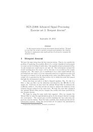
(a) BM<strong>3D</strong> with collaborative hard-thresholding<br />
(b) BM<strong>3D</strong> with collaborative Wiener filtering<br />
Figure 2. Flowcharts of the BM<strong>3D</strong> filter extentions for colored-noise removal.<br />
formed <strong>by</strong> stacking together blocks (from various image locations) which are similar to the current one. This<br />
process is called “grouping” and is realized <strong>by</strong> block-matching. Consequently, a separable <strong>3D</strong> <strong>transform</strong> T<strong>3D</strong> is<br />
applied on the <strong>3D</strong> array in such a manner that first a 2D <strong>transform</strong>, T2D, is applied on each block in the group<br />
and then a 1D <strong>transform</strong>, T1D, is applied in the third dimension. The noise is attenuated <strong>by</strong> shrinkage (e.g.<br />
hard-thresholding or empirical Wiener filtering) of the T<strong>3D</strong>-<strong>transform</strong> spectrum. Subsequently, the <strong>transform</strong><br />
T<strong>3D</strong> is inverted and each of the filtered blocks in the group is returned to its original location. After processing<br />
the whole image, since the filtered blocks can (and usually do) mutually overlap, they are aggregated <strong>by</strong> weighted<br />
averaging to form a final denoised image.<br />
If the <strong>transform</strong>s T2D and T1D are orthonormal, the grouped blocks are non-overlapping, and the noise in<br />
the input image is i.i.d. Gaussian, then the noise in the T<strong>3D</strong>-<strong>transform</strong> <strong>domain</strong> is also i.i.d. Gaussian with the<br />
(�) �<br />
same constant variance. However, if the noise is colored as in the case of Eq. (3), then the variances �2 2D<br />
for � =1������2 1 ,oftheT2D-<strong>transform</strong> coe�cients are in general non constant. In the following subsections,<br />
we extend the BM<strong>3D</strong> filter to attenuate such colored noise. We note that the developed extensions are not<br />
necessarily restricted to the considered image <strong>restoration</strong> scheme but are applicable to filtering of colored noise<br />
in general.<br />
Let us introduce the notation used in what follows. With �RI � we denote a 2D block of fixed size �1 × �1<br />
extracted from �RI ,where���is the coordinate of the top-left corner of the block. Let us note that this<br />
block notation is di�erent from the one (capital letter with subscript) used in10 since the capital letter in this<br />
paper is reserved for the DFT of an image. A group of collected 2D blocks is denoted <strong>by</strong> a bold-face letter with<br />
is a <strong>3D</strong> array composed of the blocks<br />
a subscript indicating the set of its grouped blocks’ coordinates: e.g., zRI �<br />
�RI � , �� � � � �.<br />
2.1. BM<strong>3D</strong> with collaborative hard-thresholding (Step 1.2)<br />
This filtering is applied on the noisy �RI given <strong>by</strong> Eq. (3). The variances of the coe�cients of a T2D-<strong>transform</strong><br />
(applied to an arbitrary image block) are computed as<br />
� 2 2D (�) = �2<br />
°<br />
°�<br />
|�|<br />
RI n<br />
F � (�)<br />
o°<br />
°° 2<br />
T2D<br />
2 , �� =1������2 1 , (5)
where � (�)<br />
T2D is the �-th basis element of T2D. The flowchart of the BM<strong>3D</strong> with collaborative hard-thresholding<br />
extended for color-noise attenuation is given in Figure 2(a).<br />
The variances �2 2D are used in the block-matching to reduce the influence of noisier <strong>transform</strong> coe�cients<br />
when determining the block-distance. To accomplish this, the block-distance is computed as the �2-norm of<br />
the di�erence between the two T2D-<strong>transform</strong>ed blocks scaled <strong>by</strong> the corresponding standard deviations of the<br />
T2D-<strong>transform</strong> coe�cients. Thus, the distance is given <strong>by</strong><br />
� ¡ � RI<br />
�� ��RI<br />
�<br />
¢ = � �2<br />
1<br />
°<br />
T2D<br />
© ª<br />
RI ��� � T2D<br />
�2D<br />
© � RI<br />
�<br />
ª ° 2 ° , (6)<br />
°<br />
where �RI �� is the current reference block, �RI © � is ª an arbitrary © ª block in the search neighborhood, and the operations<br />
RI<br />
RI<br />
between the three �1 × �1 arrays T2D ��� , T2D �� ,and�2D are elementwise. After the best-matching<br />
blocks are found (their coordinates are saved as the elements of the set ���) and grouped together in a <strong>3D</strong><br />
array, collaborative hard-thresholding is applied. It consists of applying the <strong>3D</strong> <strong>transform</strong> T<strong>3D</strong> on the <strong>3D</strong> group,<br />
hard-thresholding its spectrum, and then inverting the T<strong>3D</strong>. To attenuate the colored noise, the hard-threshold is<br />
made dependent on the variance of each T<strong>3D</strong>-<strong>transform</strong> coe�cient. Due to the separability of T<strong>3D</strong>, this variance<br />
depends only on the corresponding 2D coordinate within the T<strong>3D</strong>-spectrum; thus, along the third dimension of a<br />
group the variance and hence the threshold areo the same. The hard-thresholding is performed <strong>by</strong> an elementwise<br />
multiplication of the T<strong>3D</strong>-spectrum T<strong>3D</strong> with the <strong>3D</strong> array h�� defined as<br />
h�� (�� �) =<br />
(<br />
1, if<br />
n<br />
zRI ��� ¯ n<br />
¯<br />
¯T<strong>3D</strong> zRI o<br />
��� 0, otherwise,<br />
¯<br />
(�� �) ¯ ��<strong>3D</strong>�2D (�)<br />
2<br />
, �� =1������ 2 1 , �� =1�����|���| �<br />
where � is a spatial-coordinate index and � is an index of the coe�cients in the third dimension, �<strong>3D</strong> is a fixed<br />
threshold coe�cient and |���| denotes the cardinality of the set ���.<br />
After all reference blocks are processed, the filtered blocks are aggregated <strong>by</strong> a weighted averaging, producing<br />
the denoised image ˆ� RI . The weight for all filtered blocks in an arbitrary <strong>3D</strong> group is the inverse of the sum<br />
of the variances of the non-zero <strong>transform</strong> coe�cients after hard-thresholding; for a <strong>3D</strong> group using �� � � as<br />
reference, the weight is<br />
� ht<br />
�� =<br />
X<br />
�=1������ 2 1<br />
�=1�����|�� �|<br />
1<br />
h�� (�� �) �2 2D (�).<br />
2.2. BM<strong>3D</strong> with collaborative Wiener filtering (Step 2.2)<br />
The BM<strong>3D</strong> with collaborative empirical Wiener filtering uses ˆ� RI as a reference estimate of the true image �.<br />
Since the grouping <strong>by</strong> block-matching is performed on this estimate and not on the noisy image, there is no need<br />
to modify the distance calculation as in Eq. (6). The only modification from Step 2 of the original BM<strong>3D</strong> filter<br />
concerns the di�erent variances of the T<strong>3D</strong>-<strong>transform</strong> coe�cients in the empirical n oWiener<br />
filtering. This filtering<br />
RW I<br />
is performed <strong>by</strong> an elementwise multiplication of the T<strong>3D</strong>-spectrum T<strong>3D</strong> z with the Wiener attenuation<br />
��� coe�cients w�� defined as<br />
w�� (�� �) =<br />
¯<br />
¯T<strong>3D</strong><br />
¯ n<br />
¯<br />
¯T<strong>3D</strong><br />
n<br />
<strong>by</strong> RI<br />
�� �<br />
o ¯<br />
(�� �)<br />
o ¯<br />
(�� �)<br />
<strong>by</strong> RI<br />
�� �<br />
¯ 2<br />
¯ 2<br />
+ �2 2D (�)<br />
, �� =1������ 2 1 � �� =1�����|���| ,<br />
where, similarly to Eq. (5), the variances � 2 2D of the T2D-<strong>transform</strong> coe�cients are computed as<br />
� 2 2D (�) = �2<br />
°<br />
°�<br />
|�|<br />
RW I n<br />
F � (�)<br />
o° 2 °°<br />
T2D<br />
2 , �� =1������2 1 . (7)
For an arbitrary �� � �, the aggregation weight for its corresponding filtered <strong>3D</strong> group is<br />
� wie<br />
�� =<br />
X<br />
�=1������ 2 1<br />
�=1�����|�� �|<br />
1<br />
w 2 �� (�� �) �2 2D (�).<br />
The flowchart of the BM<strong>3D</strong> with collaborative Wiener filtering extended for color-noise attenuation is given in<br />
Figure 2(b).<br />
3. RESULTS AND DISCUSSION<br />
We present simulation results of the proposed algorithm, whose Matlab implementation is available online. 13<br />
All parameters, obtained after a rough empirical optimization, are fixed in all experiments (invariant of the<br />
noise variance � 2 ,blurPSF�, and image �) and can be inspected from the provided implementation. In our<br />
experiments, we used the same blur PSFs and noise combinations as in. 4 In particular, these PSFs are:<br />
• PSF 1: � (�1��2) =1� ¡ 1+�2 1 + �2 ¢<br />
2 ��1��2 = �7�����7,<br />
• PSF 2: � is a 9 × 9 uniform kernel (boxcar),<br />
• PSF 3: � =[14641] � [14641]�256,<br />
• PSF 4: � is a Gaussian PSF with standard deviation 1.6,<br />
• PSF 5: � is a Gaussian PSF with standard deviation 0.4.<br />
All PSFs are normalized so that P � =1.<br />
Table 1 presents a comparison of the improvement in signal-to-noise ratio (ISNR) for a few methods<br />
3, 4, 6, 14—16<br />
among which are the current best. 3, 4 The results of ForWaRD 6 were obtained with the Matlab codes 17 made<br />
available <strong>by</strong> its authors, for which we used automatically estimated regularization parameters. The results<br />
of the SA-DCT deblurring 3 were produced with the Matlab implementation, 18 where however we used fixed<br />
regularization parameters in all experiment in order to have fair comparison (rather than using regularization<br />
parameters dependent on the PSF and noise). The results of the GSM method 19 and the SV-GSM 4 are taken<br />
from. 4 In most of the experiments, the proposed method outperforms the other techniques in terms of ISNR. We<br />
note that the results of the four standard experiments used in the literature (e.g., 3, 6, 7, 20 ) on image <strong>restoration</strong><br />
are included in Table 1 as follows.<br />
• Experiment 1: PSF2, �2 =0�308, andCameraman image.<br />
• Experiment 2: PSF1, �2 =2,andCameraman image.<br />
• Experiment 3: PSF1, �2 =8,andCameraman image.<br />
• Experiment 4: PSF3, �2 =49,andLena image.<br />
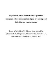
The visual quality of some of the restored images can be evaluated from Figures 4, 5, and 6. One can see<br />
that fine details are well preserved and there are few artifacts in the deblurred images. In particular, ringing can<br />
be seen in some images such as the ones shown in Figure 3, where a comparison with the SA-DCT deblurring 3<br />
is made. The ringing is stronger (and ISNR is lower) in the estimate obtained <strong>by</strong> the proposed technique. We<br />
explain this as follows; let us recall that each of the noisy images � RI and � RW I (input to the extended BM<strong>3D</strong><br />
filter) is sum of a bias and additive colored noise; the exact models of � RI and � RW I are given <strong>by</strong> Eq. (3) and<br />
(4), respectively. The ringing is part of the bias and thus it is not modeled as additive colored noise. Hence, if<br />
the ringing magnitude is relatively high, the BM<strong>3D</strong> fails to attenuate it and it is preserved in the final estimate,<br />
as in Figure 3.<br />
By comparing the results corresponding to ˆ� RI and ˆ� RW I in Table 2, one can see the improvement in ISNR<br />
after applying the second step (RWI using BM<strong>3D</strong> with collaborative Wiener filtering) of our two-step <strong>restoration</strong><br />
scheme. This improvement is significant and can be explained as follows. First, the regularized Wiener inverse is<br />
more e�ective than the regularized inverse because it uses the estimated power spectrum for the inversion given
Blur: PSF2, � 2 =0�308 SA-DCT deblurring 3 Proposed method<br />
(PSNR 20.76 dB) (ISNR 8.55 dB) (ISNR 8.34 dB)<br />
Fragments of the SA-DCT result Fragments of the result <strong>by</strong> the proposed method<br />
Figure 3. Comparison of the proposed method with the SA-DCT deconvolution method for Cameraman and PSF 2 blur<br />
kernel.<br />
in Eq. (4). Second, the block-matching in the BM<strong>3D</strong> filtering is more accurate because it is performed within<br />
the available estimate ˆ� RI rather than within the input noisy image �RW I . Third, the empirical Wiener filtering<br />
used <strong>by</strong> the BM<strong>3D</strong> in that step is more e�ective than the simple hard-thresholding used in the first step. In<br />
fact, the first step can be considered as an adaptation step that significantly improves the actual <strong>restoration</strong><br />
performed <strong>by</strong> the second step.<br />
RW I<br />
In Table 2, we also provide (in the row corresponding to ˆ� naive ) the results of the naive approach of using the<br />
original BM<strong>3D</strong> filter10 rather than the one extended for colored noise. This filter was applied on �RI RW I and �<br />
<strong>by</strong> assuming additive i.i.d. Gaussian noise, whose variance was computed as �2 �2 P 2<br />
�1 WGN = �1 �=1 �22D (�), where<br />
�2 2D (·) is defined in Eq. (5) and (7) for �RI and �RW I , respectively. This variance calculation was empirically<br />
found to be better (in terms of ISNR) than estimating a noise variance from the noisy images �RI and �RW I .<br />
The benefit of using the BM<strong>3D</strong> for colored noise reaches 1 dB; in particular, the benefit is substantial for those<br />
experiments where the noise in �RI and �RW I is highly colored.<br />
4. CONCLUSIONS<br />
The developed image deblurring method outperforms the current best techniques in most of the experiments.<br />
This performance is in line with the BM<strong>3D</strong> denoising filter10 which is among the current best denoising filters.<br />
The proposed colored-noise extension of the BM<strong>3D</strong> is not restricted to the developed deblurring method and it<br />
can in general be applied to filter colored noise.<br />
Future developments might target attenuation of ringing artifacts <strong>by</strong> exploiting the SA-DCT <strong>transform</strong>21 which,asshowninFigure3,ise�ective in suppressing them.
Blur PSF 1 PSF 2 PSF 3 PSF 4 PSF 5<br />
� 2 2 8 0�308 49 4 64<br />
Cameraman<br />
Input PSNR 22.23 22.16 20.76 24.62 23.36 29.82<br />
ForWaRD 6 6.76 5.08 7.34 2.40 3.14 3.92<br />
GSM 19 6.84 5.29 -1.61 2.56 2.83 3.81<br />
EM 16 6.93 4.88 7.59 - - -<br />
Segm.-based Reg. 15 7.23 - 8.04 - - -<br />
GEM 14 7.47 5.17 8.10 - - -<br />
BOA 20 7.46 5.24 8.16 - - -<br />
Anis. LPA-ICI 7 7.82 5.98 8.29 - - -<br />
SV-GSM 4 7.45 5.55 7.33 2.73 3.25 4.19<br />
SA-DCT 3 8.11 6.33 8.55 3.37 3.72 4.71<br />
Proposed 8.19 6.40 8.34 3.34 3.73 4.70<br />
Lena<br />
Input PSNR 27.25 27.04 25.84 28.81 29.16 30.03<br />
Segm.-based Reg. 15 - - - 1.34 - -<br />
GEM 14 - - - 2.73 - -<br />
BOA 20 - - - 2.84 - -<br />
ForWaRD 6 6.05 4.90 6.97 2.93 3.50 5.42<br />
EM 16 - - - 2.94 - -<br />
Anis. LPA-ICI 7 - - - 3.90 - -<br />
SA-DCT 3 7.55 6.10 7.79 4.49 4.08 5.84<br />
Proposed 7.95 6.53 7.97 4.81 4.37 6.40<br />
House<br />
Input PSNR 25.61 25.46 24.11 28.06 27.81 29.98<br />
ForWaRD 6 7.35 6.03 9.56 3.19 3.85 5.52<br />
GSM 19 8.46 6.93 -0.44 4.37 4.34 5.98<br />
SV-GSM 4 8.64 7.03 9.04 4.30 4.11 6.02<br />
SA-DCT 3 9.02 7.74 10.50 4.99 4.65 5.96<br />
Proposed 9.32 8.14 10.85 5.13 4.56 7.21<br />
Barbara<br />
Input PSNR 23.34 23.25 22.49 24.22 23.77 29.78<br />
ForWaRD 6 3.69 1.87 4.02 0.94 0.98 3.15<br />
GSM 19 5.70 3.28 -0.27 1.44 0.95 4.91<br />
SV-GSM 4 6.85 3.80 5.07 1.94 1.36 5.27<br />
SA-DCT 3 5.45 2.54 4.79 1.31 1.02 3.83<br />
Proposed 7.80 3.94 5.86 1.90 1.28 5.80<br />
Table 1. Comparison of the output ISNR [dB] of a few deconvolution methods (only the rows corresponding to “Input<br />
PSNR” contain PSNR [dB] of the input blurry images).
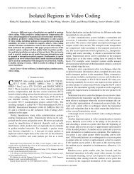
Blur: PSF1, � 2 =2 Output ISNR 9.32 dB<br />
Blur: PSF1, � 2 =8 Output ISNR 8.14 dB<br />
Blur: PSF2, � 2 =0�308 Output ISNR 10.85 dB<br />
Figure 4. Deblurring results of the proposed method for House.
Blur: PSF3, � 2 =49 Output ISNR 4.81 dB<br />
Blur: PSF4, � 2 =4 Output ISNR 4.37 dB<br />
Blur: PSF5, � 2 =64 Output ISNR 6.40 dB<br />
Figure 5. Deblurring results of the proposed method for Lena.
Blur: PSF1, � 2 =8 Output ISNR 3.94 dB<br />
Blur: PSF2, � 2 =0�308 Output ISNR 5.86 dB<br />
Blur: PSF3, � 2 =49 Output ISNR 1.90 dB<br />
Figure 6. Deblurring results of the proposed method for Barbara.
Blur � PSF 1 PSF 2 PSF 3 PSF 4 PSF 5<br />
�2 � 2 8 0�308 49 4 64<br />
ˆ� RI 7.13 5.16 7.52 2.31 3.23 2.46<br />
ˆ� RW I 8.19 6.40 8.34 3.34 3.73 4.70<br />
RW I ˆ� naive 7.17 6.25 8.14 2.57 2.71 4.63<br />
Table 2. ISNR comparison for: the basic estimate ˆ� RI ; the final estimate ˆ� RW I RW I<br />
; the final estimate ˆ� naive obtained using<br />
the original BM<strong>3D</strong> filter instead of the one extended for colored noise. The test image was Cameraman.<br />
REFERENCES<br />
1. C. Vogel, Computational Methods for Inverse Problems, SIAM, 2002.<br />
2. P. C. Hansen, Rank-Deficient and Discrete Ill-Posed Problems: Numerical Aspects of Linear Inversion,<br />
SIAM, Philadelphia, 1997.<br />
3. A. Foi, K. Dabov, V. Katkovnik, and K. Egiazarian, “Shape-Adaptive DCT for denoising and image reconstruction,”<br />
in Proc. SPIE Electronic Imaging: Algorithms and Systems V, 6064A-18, (San Jose, CA,<br />
USA), January 2006.<br />
4. J. A. Guerrero-Colon, L. Mancera, and J. Portilla, “<strong>Image</strong> <strong>restoration</strong> using space-variant Gaussian scale<br />
mixtures in overcomplete pyramids,” IEEE Trans. <strong>Image</strong> Process. 17, pp. 27—41, January 2007.<br />
5. R. Neelamani, H. Choi, and R. G. Baraniuk, “Wavelet-<strong>domain</strong> regularized deconvolution for ill-conditioned<br />
systems,” in Proc. IEEE Int. Conf. <strong>Image</strong> Process., 1, pp. 204—208, (Kobe, Japan), October 1999.<br />
6. R. Neelamani, H. Choi, and R. G. Baraniuk, “Forward: Fourier-wavelet regularized deconvolution for illconditioned<br />
systems,” IEEE Trans. Signal Process. 52, pp. 418—433, February 2004.<br />
7. V. Katkovnik, A. Foi, K. Egiazarian, and J. Astola, “Directional varying scale approximations for anisotropic<br />
signal processing,” in Proc. European Signal Process. Conf., pp. 101—104, (Vienna, Austria), September 2004.<br />
8. V. Katkovnik, K. Egiazarian, and J. Astola, “A spatially adaptive nonparametric regression image deblurring,”<br />
IEEE Trans. <strong>Image</strong> Process. 14, pp. 1469—1478, October 2005.<br />
9. V. Katkovnik, K. Egiazarian, and J. Astola, Local Approximation Techniques in Signal and <strong>Image</strong> Process.,<br />
vol. PM157, SPIE Press, 2006.<br />
10. K. Dabov, A. Foi, V. Katkovnik, and K. Egiazarian, “<strong>Image</strong> denoising <strong>by</strong> <strong>sparse</strong> <strong>3D</strong> <strong>transform</strong>-<strong>domain</strong><br />
collaborative filtering,” IEEE Trans. <strong>Image</strong> Process. 16, pp. 2080—2095, August 2007.<br />
11. A. Buades, B. Coll, and J. M. Morel, “A review of image denoising algorithms, with a new one,” Multiscale<br />
Modeling and Simulation 4(2), pp. 490—530, 2005.<br />
12. C. Kervrann and J. Boulanger, “Optimal spatial adaptation for patch-based image denoising,” IEEE Trans.<br />
<strong>Image</strong> Process. 15, pp. 2866—2878, October 2006.<br />
13. K. Dabov and A. Foi, “BM<strong>3D</strong> Filter Matlab Demo Codes.” http://www.cs.tut.fi/˜foi/GCF-BM<strong>3D</strong>.<br />
14. J. Dias, “Fast GEM wavelet-based image deconvolution algorithm,” in Proc. IEEE Int. Conf. <strong>Image</strong> Process.,<br />
3, pp. 961—964, (Barcelona, Spain), September 2003.<br />
15. M. Mignotte, “An adaptive segmentation-based regularization term for image <strong>restoration</strong>,” in Proc. IEEE<br />
Int. Conf. <strong>Image</strong> Process., 1, pp. 901—904, (Genova, Italy), September 2005.<br />
16. M. A. T. Figueiredo and R. D. Nowak, “An EM algorithm for wavelet-based image <strong>restoration</strong>,” IEEE<br />
Trans. <strong>Image</strong> Process. 12, pp. 906—916, August 2003.<br />
17. R. Neelamani, “Fourier-Wavelet Regularized Deconvolution (ForWaRD) Software for 1-D Signals and <strong>Image</strong>s.”<br />
http://www.dsp.rice.edu/software/ward.shtml.<br />
18. A. Foi and K. Dabov, “Pointwise Shape-Adaptive DCT Demobox.” http://www.cs.tut.fi/˜foi/SA-DCT.<br />
19. J. Portilla and E. P. Simoncelli, “<strong>Image</strong> <strong>restoration</strong> using Gaussian scale mixtures in the wavelet <strong>domain</strong>,”<br />
in Proc. IEEE Int. Conf. <strong>Image</strong> Process., 2, pp. 965—968, (Barcelona, Spain), September 2003.<br />
20. M. A. T. Figueiredo and R. Nowak, “A bound optimization approach to wavelet-based image deconvolution,”<br />
in Proc. IEEE Int. Conf. <strong>Image</strong> Process., 2, pp. 782—785, (Genova, Italy), September 2005.<br />
21. A. Foi, V. Katkovnik, and K. Egiazarian, “Pointwise Shape-Adaptive DCT for high-quality denoising and<br />
deblocking of grayscale and color images,” IEEE Trans. <strong>Image</strong> Process. 16, pp. 1395—1411, May 2007.