Discrete Shearlet Transform : New Multiscale Directional Image ...
Discrete Shearlet Transform : New Multiscale Directional Image ...
Discrete Shearlet Transform : New Multiscale Directional Image ...

Create successful ePaper yourself
Turn your PDF publications into a flip-book with our unique Google optimized e-Paper software.
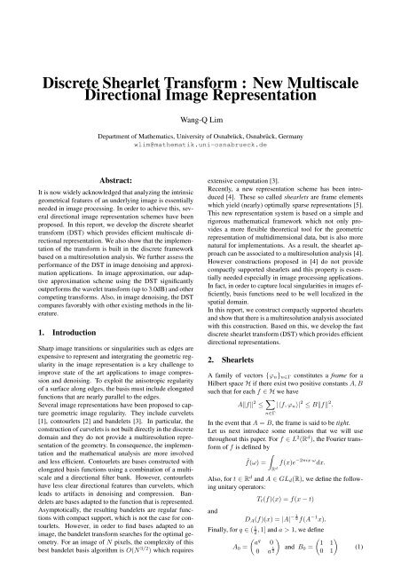
<strong>Discrete</strong> <strong>Shearlet</strong> <strong>Transform</strong> : <strong>New</strong> <strong>Multiscale</strong><br />
<strong>Directional</strong> <strong>Image</strong> Representation<br />
Wang-Q Lim<br />
Department of Mathematics, University of Osnabrück, Osnabrück, Germany<br />
wlim@mathematik.uni-osnabrueck.de<br />
Abstract:<br />
It is now widely acknowledged that analyzing the intrinsic<br />
geometrical features of an underlying image is essentially<br />
needed in image processing. In order to achieve this, several<br />
directional image representation schemes have been<br />
proposed. In this report, we develop the discrete shearlet<br />
transform (DST) which provides efficient multiscale directional<br />
representation. We also show that the implementation<br />
of the transform is built in the discrete framework<br />
based on a multiresolution analysis. We further assess the<br />
performance of the DST in image denoising and approximation<br />
applications. In image approximation, our adaptive<br />
approximation scheme using the DST significantly<br />
outperforms the wavelet transform (up to 3.0dB) and other<br />
competing transforms. Also, in image denoising, the DST<br />
compares favorably with other existing methods in the literature.<br />
1. Introduction<br />
Sharp image transitions or singularities such as edges are<br />
expensive to represent and intergrating the geometric regularity<br />
in the image representation is a key challenge to<br />
improve state of the art applications to image compression<br />
and denoising. To exploit the anisotropic regularity<br />
of a surface along edges, the basis must include elongated<br />
functions that are nearly parallel to the edges.<br />
Several image representations have been proposed to capture<br />
geometric image regularity. They include curvelets<br />
[1], contourlets [2] and bandelets [3]. In particular, the<br />
construction of curvelets is not built directly in the discrete<br />
domain and they do not provide a multiresolution representation<br />
of the geometry. In consequence, the implementation<br />
and the mathematical analysis are more involved<br />
and less efficient. Contourlets are bases constructed with<br />
elongated basis functions using a combination of a multiscale<br />
and a directional filter bank. However, contourlets<br />
have less clear directional features than curvelets, which<br />
leads to artifacts in denoising and compression. Bandelets<br />
are bases adapted to the function that is represented.<br />
Asymptotically, the resulting bandelets are regular functions<br />
with compact support, which is not the case for contourlets.<br />
However, in order to find bases adapted to an<br />
image, the bandelet transform searches for the optimal geometry.<br />
For an image of N pixels, the complexity of this<br />
best bandelet basis algorithm is O(N 3/2 ) which requires<br />
extensive computation [3].<br />
Recently, a new representation scheme has been introduced<br />
[4]. These so called shearlets are frame elements<br />
which yield (nearly) optimally sparse representations [5].<br />
This new representation system is based on a simple and<br />
rigorous mathematical framework which not only provides<br />
a more flexible theoretical tool for the geometric<br />
representation of multidimensional data, but is also more<br />
natural for implementations. As a result, the shearlet approach<br />
can be associated to a multiresolution analysis [4].<br />
However constructions proposed in [4] do not provide<br />
compactly supported shearlets and this property is essentially<br />
needed especially in image processing applications.<br />
In fact, in order to capture local singularities in images efficiently,<br />
basis functions need to be well localized in the<br />
spatial domain.<br />
In this report, we construct compactly supported shearlets<br />
and show that there is a multiresolution analysis associated<br />
with this construction. Based on this, we develop the fast<br />
discrete shearlet transform (DST) which provides efficient<br />
directional representations.<br />
2. <strong>Shearlet</strong>s<br />
A family of vectors {ϕn}n∈Γ constitutes a frame for a<br />
Hilbert space H if there exist two positive constants A, B<br />
such that for each f ∈ H we have<br />
A�f� 2 ≤ �<br />
|〈f, ϕn〉| 2 ≤ B�f� 2 .<br />
n∈Γ<br />
In the event that A = B, the frame is said to be tight.<br />
Let us next introduce some notations that we will use<br />
throughout this paper. For f ∈ L2 (Rd ), the Fourier transform<br />
of f is defined by<br />
�<br />
ˆf(ω) = f(x)e −2πix·ω dx.<br />
R d<br />
Also, for t ∈ R d and A ∈ GLd(R), we define the following<br />
unitary operators:<br />
and<br />
Tt(f)(x) = f(x − t)<br />
1 −<br />
DA(f)(x) = |A| 2 f(A −1 x).<br />
Finally, for q ∈ ( 1<br />
2 , 1] and a > 1, we define<br />
�<br />
� �<br />
1 1<br />
A0 =<br />
and B0 =<br />
0 1<br />
� q a 0<br />
0 a 1<br />
2<br />
(1)
and<br />
A1 =<br />
� 1<br />
a 2 0<br />
0 aq �<br />
and B1 =<br />
� �<br />
1 0<br />
. (2)<br />
1 1<br />
We are now ready to define a shearlet frame as follows.<br />
For c ∈ R + , ψ 1 0, . . . , ψ L 0 , ψ 1 1, . . . , ψ L 1 ∈ L 2 (R 2 ) and φ ∈<br />
L 2 (R 2 ), we define<br />
and<br />
Ψ 0 c = {ψ i,0<br />
jkm : j, k ∈ Z, m ∈ Z2 , i = 1, . . . , L},<br />
Ψ 1 c = {ψ i,1<br />
jkm : j, k ∈ Z, m ∈ Z2 , i = 1, . . . , L},<br />
Ψ 2 c = {Tcmφ : m ∈ Z 2 }<br />
∪{ψ i,0<br />
jkm : j ≥ 0, −2j ≤ k ≤ 2 j , m ∈ Z 2 , i = 1, . . . , L}<br />
∪{ψ i,1<br />
jkm : j ≥ 0, −2j ≤ k ≤ 2 j , m ∈ Z 2 , i = 1, . . . , L}<br />
where<br />
ψ i,ℓ<br />
jkm = D A −j<br />
ℓ B−k<br />
Tcmψ<br />
ℓ<br />
i ℓ<br />
for ℓ = 0, 1, m ∈ Z2 , i = 1, . . . , L and j, k ∈ Z. If Ψp c<br />
is a frame for L2 (R2 ), then we call the functions ψ i,ℓ<br />
jkm in<br />
the system Ψp c shearlets.<br />
(3)<br />
Observe that each element ψ i,ℓ<br />
jkm in Ψp c is obtained by ap-<br />
plying an anisotropic scaling matrix Aℓ and a shear ma-<br />
. This implies that<br />
trix Bℓ to fixed generating functions ψi ℓ<br />
the system Ψp c can provide window functions which can<br />
be elongated along arbitrary directions. Therefore, the<br />
geometrical structures of singularities in images can be<br />
efficiently represented and analyzed using those window<br />
functions. In fact, it was shown that 2-dimensional piecewise<br />
smooth functions with C2-singularities can be approximated<br />
with nearly optimal approximation rate using<br />
shearlets. We refer to [5] for details. Furthermore, one<br />
can show that shearlets can completely analyze the singular<br />
structures of piecewise smooth images [6]. In fact,<br />
this property of shearlets is useful especially in signal and<br />
image processing, since singularities and irregular structures<br />
carry essential information in a signal. For example,<br />
discontinuities in the intensity of an image indicate the<br />
presence of edges. Figure 1 displays examples of shearlets<br />
which can be elongated along arbitrary direction in<br />
the spatial domain.<br />
3. Construction of <strong>Shearlet</strong>s<br />
In this section, we will introduce some useful sufficient<br />
conditions to construct compactly supported shearlets.<br />
Using these conditions, we will show that the system Ψ p c<br />
can be generated by simple separable functions associated<br />
with a multiresolution analysis. Furthermore, this leads to<br />
the fast DST, and we will discuss this in the next section.<br />
We first discuss sufficient conditions for the existence<br />
of compactly supported shearlets. � For this, � let α ><br />
α+1<br />
max (1, (1 − p)γ) and γ > max<br />
be fixed<br />
p , 1<br />
1−p<br />
positive numbers for 0 < p < 1. We choose α ′ , γ ′ > 0<br />
such that α ′ ≥ α+γ and γ ′ ≥ α ′ −α+γ. Then we obtain<br />
the following results [7].<br />
Figure 1: Examples of shearlets in the spatial domain. The<br />
top row illustrates shearlet functions ψ i,0<br />
associated with<br />
jk0<br />
matrices A0 and B0 in (1). The bottom row shows shearlet<br />
functions ψ i,1<br />
jk0 associated with matrices A1 and B1 in (2)..<br />
Theorem 3..1. [7] For i = 1, . . . , L, we define<br />
ψ i 0(x1, x2) = γ i (x1)θ(x2) such that<br />
and<br />
If<br />
and<br />
|ω1| α′<br />
|ˆγ i (ω1)| ≤ K1<br />
(1 + |ω1| 2 ) γ′ /2<br />
| ˆ θ(ω1)| ≤ K2(1 + |ω1| 2 ) −γ′ /2 .<br />
ess inf<br />
|ω1|≤1/2 |ˆ θ(ω1)| 2 ≥ K3 > 0 (4)<br />
ess inf<br />
a−q≤|ω1|≤1 i=1<br />
L�<br />
|ˆγ i (ω1)| 2 ≥ K4 > 0, (5)<br />
then there exists c0 > 0 such that Ψ 0 c is a frame for L 2 (R 2 )<br />
for all c ≤ c0.<br />
Observe that the functions ψ 1 0, . . . , ψ L 0 are separable functions,<br />
and the one-dimensional scaling function θ and<br />
wavelets γ i can be chosen with sufficient vanishing moments<br />
in this case.<br />
We now show some concrete examples of compactly supported<br />
shearlets using Theorem 3.1. Assume that a = 4<br />
and q = 1 in (1) and (2). Let us consider a box spline [1]<br />
of order m defined as follows.<br />
�<br />
ˆθm(ω1)<br />
sin<br />
�<br />
πω1 m+1<br />
=<br />
e<br />
πω1<br />
−iɛω1 ,<br />
where ɛ = 1 if m is even, and ɛ = 0 if m is odd. Obviously,<br />
we have the following two scaling equation:<br />
and<br />
ˆθm(2ω1) = m0(ω1) ˆ θm(ω1)<br />
m0(ω1) = (cos πω1) m+1 e −iɛπω1 .<br />
Let α ′ and γ ′ be positive real numbers as in Theorem 3.1.<br />
We now define<br />
and<br />
ˆψ 1 0(ω) = (i) ℓ√ � �ℓ 2 sin πω1<br />
ˆθm(ω1) ˆ θm(ω2)<br />
ˆψ 2 0(ω) = (i) ℓ�<br />
sin πω1<br />
2<br />
� ℓ ˆθm( ω1<br />
2 )ˆ θm(ω2),
where ℓ ≥ α ′ and m + 1 ≥ γ ′ . Then, by Theorem 3.1, ψ 1 0<br />
and ψ 2 0 generate a frame Ψ 0 c for c ≤ c0 with some c0 > 0.<br />
There are infinitely many possible choices for ℓ and m.<br />
For example, one can choose ℓ = 9 and m = 11.<br />
Define<br />
and<br />
φ(x1, x2) = θm(x1)θm(x2),<br />
ˆψ 1 1(ω) = (i) ℓ√ � �ℓ 2 sin πω2<br />
ˆθm(ω2) ˆ θm(ω1)<br />
ˆψ 2 1(ω) = (i) ℓ�<br />
sin πω2<br />
2<br />
� ℓ ˆθm( ω2<br />
2 )ˆ θm(ω1).<br />
Then similar arguments show that ψ 1 1 and ψ 2 1 generate a<br />
frame Ψ1 c for c ≤ c0 with some c0 > 0. Furthermore, the<br />
functions φ, ψi ℓ for ℓ = 0, 1 and i = 1, 2 generate a frame<br />
Ψ2 c with c ≤ c0 for some c0 > 0.<br />
4. <strong>Discrete</strong> <strong>Shearlet</strong> <strong>Transform</strong><br />
In the previous section, we constructed compactly supported<br />
shearlets generated by separable functions associated<br />
with a multiresolution analysis. In this section, we<br />
will show that this multiresolution analysis leads to the<br />
fast DST which computes 〈f, ψ i,ℓ<br />
jkm<br />
〉. To be more specific,<br />
we let a = 4 and q = 1 in (1) and (2). For notational<br />
convenience, we let n = (n1, n2), m = (m1, m2), d =<br />
(d1, d2) ∈ Z 2 and I2 be a 2 by 2 identity matrix.<br />
Let θ ∈ L 2 (R) be a compactly supported function such<br />
that {θ(· − n1) : n1 ∈ Z} is an orthonormal sequence and<br />
Define<br />
θ(x1) = �<br />
h(n1) √ 2θ(2x1 − n1). (6)<br />
n1∈Z<br />
γ(x1) = �<br />
g(n1) √ 2θ(2x1 − n1) (7)<br />
n1∈Z<br />
such that γ has sufficient vanishing moments and the pair<br />
of the filters h and g is a pair of conjugate mirror filters.<br />
We assume that γ and θ satisfy decay conditions (4) and<br />
(5) in Theorem 3.1. We also define<br />
and<br />
φ(x1, x2) = θ(x1)θ(x2),<br />
ψ 1 ℓ (x1, x2) = γ(xℓ+1)θ(x2−ℓ) (8)<br />
ψ 2 1 −<br />
ℓ (x1, x2) = 2 2 γ( xℓ+1<br />
2 )θ(x2−ℓ) (9)<br />
for ℓ = 0, 1. Then Theorem 3.1 can be easily generalized<br />
to show that the functions ψ1 0, ψ2 0, ψ1 1, ψ2 1 and φ generate a<br />
shearlet frame Ψ2 c with c < c0 for some c0 > 0.<br />
Let J be a positive odd integer. Based on a multiresolution<br />
analysis associated with the two-scale equation (6), we can<br />
now easily derive a fast algorithm for computing shearlet<br />
coefficients 〈f, ψ i,ℓ<br />
J−1<br />
jkm 〉 for ℓ = 0, 1,j = 1, . . . , 2 , and<br />
−2j ≤ k ≤ 2j as follows.<br />
First, assume that<br />
f = �<br />
fJ(n)D2−J I2Tnφ (10)<br />
n∈Z 2<br />
Figure 2: Examples of anisotropic discrete wavelet decomposition:<br />
(a) Anisotropic discrete wavelet decomposition<br />
by W, (b) Anisotropic discrete wavelet decomposition<br />
by � W.<br />
where fJ(n) = 〈 f, D2−J I2Tnφ 〉. For h = 0, 1, let us<br />
define maps D k,j<br />
h : ℓ2 (Z2 ) → ℓ2 (Z2 ) by<br />
(D k,j<br />
�<br />
h x)(d) =<br />
m∈Z2 d k,j<br />
h (d, m)x(m)<br />
where d k,j<br />
h (d, m) = 〈 D B k/2j Tmφ, Tdφ 〉 and x ∈ ℓ(Z<br />
h<br />
2 ).<br />
Also we define<br />
H(ω1) = �<br />
h(n1)e −2iπω1<br />
and<br />
n1<br />
G(ω1) = �<br />
g(n1)e −2iπω1 .<br />
n1<br />
Finally, we let hj, g0 j and g1 j be the Fourier coefficients of<br />
⎧<br />
⎪⎨ Hj(ω2) =<br />
⎪⎩<br />
�J−j−1 k=0 H<br />
�<br />
2k �<br />
ω2 for J − j > 0,<br />
G0 j (ω1) = �J−2j−2 k=0 H(2kω1)G(2J−2j−1ω1), G1 j (ω1) = �J−2j−1 k=0 H(2kω1)G(2J−2jω1), (11)<br />
respectively. Then we obtain<br />
⎧<br />
〈f, ψ<br />
⎪⎨<br />
⎪⎩<br />
1,0<br />
jkm 〉 = (((Dk,j 0 fJ) ∗r hj) ↓2J−j ∗c g0 j) ↓2J−2j (m),<br />
〈f, ψ 2,0<br />
jkm<br />
〈f, ψ 1,1<br />
jkm 〉 = (((Dk,j 1 fJ) ∗c hj) ↓2J−j ∗r g0 j) ↓2J−2j (m),<br />
〈f, ψ 2,1<br />
jkm<br />
〉 = (((Dk,j<br />
0 fJ) ∗r hj) ↓2 J−j ∗c g 1 j) ↓2 J−2j+1(m),<br />
〉 = (((Dk,j<br />
1 fJ) ∗c hj) ↓2 J−j ∗r g 1 j) ↓2 J−2j+1(m),<br />
(12)<br />
where ∗c and ∗r are convolutions along the vertical and<br />
horizontal axes respectively, ↓ 2 j is the downsampling by<br />
2 j and h(n) = h(−n) for given filter coefficients h(n).<br />
From (12), we observe that the shearlet transform<br />
〈f, ψ i,ℓ<br />
jkm 〉 is the application of the shear transformation<br />
to f ∈ L2 (R2 ) followed by the wavelet transform<br />
D B k/2 j<br />
ℓ<br />
associated with anisotropic scaling matrix Aℓ. In this case,<br />
applying D k,j<br />
ℓ to fJ ∈ ℓ2 (Z2 ) corresponds to applying<br />
in the discrete domain. Thus<br />
the shear transform D B k/2 j<br />
ℓ<br />
we simply replace the operator D k,j<br />
ℓ by the discrete shear<br />
transform P ℓ k,j for fJ ∈ ℓ2 (Z2 ), where we define the discrete<br />
shear transforms P 0 k,j and P 1 k,j as follows:<br />
�<br />
�<br />
n1 + ⌊(k/2j �<br />
)n2⌋, n2 ,<br />
(P 0 k,jfJ)(n) = fJ<br />
(P 1 k,jfJ)(n) = fJ<br />
� n1, n2 + ⌊(k/2 j )n1⌋ � .<br />
(13)<br />
Let M be a fixed positive integer. Since P 0 k,j and P 1 k,j<br />
are unitary operators on ℓ(Z 2 ), we can extend the shearlet
transform defined in (12) to a linear transform S consisting<br />
of finitely many orthogonal transforms S M k and ˜ S M k where<br />
S M k (fJ) = WP 0 k,M (fJ) and ˜ S M k (fJ) = � WP 1 k,M (fJ)<br />
and W and � W are the wavelet transform associated with<br />
an anisotropic sampling matrices A0 and A1, respectively.<br />
For the precise definitions of W and � W, we refer to [7].<br />
In this case, the linear transform S, which we call DST, is<br />
defined by<br />
S = (S M<br />
−2M , . . . , SM<br />
2M , ˜ S M<br />
−2M , . . . , ˜ S M<br />
2M )<br />
for a given M ∈ Z + . Notice that redundancy of the DST<br />
is K = 2 M+2 + 2 and the DST merely requires O(KN)<br />
operations for an image of N pixels. It is obvious that the<br />
inverse DST is simply the adjoint of S with normalization.<br />
5. <strong>Image</strong> Approximation Using DST<br />
In this section, we present some results of the DST in image<br />
compression applications. In this case, we use adaptive<br />
image representation using the DST. The main idea of<br />
this is similar to the matching pursuit introduced by Mallat<br />
and Zhong [8]. The matching pursuit selects vectors one<br />
by one from a given basis dictionary at each iteration step.<br />
On the other hand, our approximation scheme searches the<br />
optimal directional index k0 at each iteration step so that<br />
corresponding the orthogonal transform S M k0 or ˜ S M k0 provides<br />
an optimal nonlinear approximation with P nonzero<br />
terms among all possible 2 M+2 + 2 orthogonal transforms<br />
in S. For a detailed description of this algorithm, we refer<br />
to [7]. For numerical tests, we compare the performance<br />
of the DST to other transforms such as the discrete<br />
biorthogonal CDF 9/7 wavelet transform (DWT)[9] and<br />
contourlet transform (CT)[2] in image compression (see<br />
Figure 3). We used only 2 directions (horizontal and vertical)<br />
and 4 level decomposition for our DST. In this case,<br />
our numerical tests indicate that only a few iterations (1-<br />
5) can give significant improvement over other transforms<br />
and computing time is comparable to the wavelet transform.<br />
For more results, we refer to [8].<br />
6. Conclusion<br />
We have constructed compactly supported shearlet systems<br />
which can provide efficient directional image representations.<br />
We also have developed the fast discrete implementation<br />
of shearlets called the DST. This algorithm<br />
consists of applying the shear transforms in the discrete<br />
domain followed by the anisotropic wavelet transforms.<br />
Applications of our proposed transform in image approximation<br />
and denoising were studied. In image approximation,<br />
the results obtained with our adaptive image representation<br />
using the DST are significantly superior to those<br />
of other transforms such as the DWT and CT both visually<br />
and with respect to PSNR.<br />
In denoising, we studied the performance of the DST coupled<br />
with a (partially) translation invariant hard tresholding<br />
estimator. Our results indicate that the DST consistently<br />
outperforms other competing transforms. For detailed<br />
numerical results, we refer to [7].<br />
Figure 3: Compression results of ’Barbara’ image of<br />
size 512 × 512: The image is reconstructed from 5024<br />
most significant coefficients. Top left: Zoomed original<br />
image, Top right: Zoomed image reconstructed by the<br />
DWT (PSNR = 25.11), Bottom left: Zoomed image reconstructed<br />
by the CT (PSNR = 25.88), Bottom right:<br />
Zoomed image reconstructed by the DST with only 1 iteration<br />
step (PSNR = 26.73).<br />
References:<br />
[1] E. Candes and D. Donoho, ”<strong>New</strong> tight frames of<br />
curvelets and optimal representations of objects<br />
with piecewise C 2 singularities,” Commun. Pure<br />
Appl. Math, vol. 57, no. 2, pp. 219-266, Feb. 2004.<br />
[2] M. Do and M. Vetterli, ”The contourlet transform:<br />
An efficient directional multiresolution image representation,”<br />
IEEE Trans. <strong>Image</strong> Process., vol. 14,<br />
no. 12, pp. 2091-2106, Dec. 2005.<br />
[3] G. Peyre and S. Mallat, ”<strong>Discrete</strong> Bandelets with<br />
Geometric Orthogonal Filters,” Proceedings of<br />
ICIP, Sept. 2005.<br />
[4] D. Labate, W. Lim, G. Kutyniok and G. Weiss<br />
”Sparse Multidimensional Representation using<br />
<strong>Shearlet</strong>s”, Proc. of SPIE conference on Wavelet<br />
Applications in Signal and <strong>Image</strong> Processing XI,<br />
San Diego, USA, 2005.<br />
[5] K. Guo and D. Labate, ”Optimally Sparse Multidimensional<br />
Representation using <strong>Shearlet</strong>s,”, SIAM<br />
J Math. Anal., 39 pp. 298-318, 2007.<br />
[6] K. Guo, D. Labate and W. Lim, ”Edge Analysis and<br />
identification using the Continuous <strong>Shearlet</strong> <strong>Transform</strong>”,<br />
to appear in Appl. Comput. Harmon. Anal.<br />
[7] W. Lim, ”Compactly Supported <strong>Shearlet</strong> Frames<br />
and Their Applications”, submitted.<br />
[8] S. Mallat and S. Zhang, ”Matching Pursuits With<br />
Time-Frequency Dictionaries,” IEEE Trans. Signal<br />
Process., pp. 3397-3415, Dec. 1993.<br />
[9] A. Cohen, I. Daubechies and J. Feauveau,<br />
”Biorthogonal bases of compactly supported<br />
wavelets,” Commun. on Pure and Appl. Math.,<br />
45:485-560, 1992.