Documenta Mathematica Optimization Stories - Mathematics

Documenta Mathematica 

Journal der 

Deutschen Mathematiker-Vereinigung 

Gegründet 1996 

Extra Volume 

Optimization Stories 

21st International Symposium on Mathematical Programming 

Berlin, August 19–24, 2012 

Editor: 

Martin Grötschel

Documenta Mathematica, Journal der Deutschen Mathematiker-Vereinigung, 

veröffentlicht Forschungsarbeiten aus allen mathematischen Gebieten und wird in 

traditioneller Weise referiert. Es wird indiziert durch Mathematical Reviews, Science 

Citation Index Expanded, Zentralblatt für Mathematik. 

Artikel können als TEX-Dateien per E-Mail bei einem der Herausgeber eingereicht 

werden. Hinweise für die Vorbereitung der Artikel können unter der unten angegebenen 

WWW-Adresse gefunden werden. 

Documenta Mathematica, Journal der Deutschen Mathematiker-Vereinigung, 

publishes research manuscripts out of all mathematical fields and is refereed in the 

traditional manner. It is indexed in Mathematical Reviews, Science Citation Index 

Expanded, Zentralblatt für Mathematik. 

Manuscripts should be submitted as TEX -files by e-mail to one of the editors. Hints 

for manuscript preparation can be found under the following web address. 

http://www.math.uni-bielefeld.de/documenta 

Geschäftsführende Herausgeber / Managing Editors: 

Alfred K. Louis, Saarbrücken louis@num.uni-sb.de 

Ulf Rehmann (techn.), Bielefeld rehmann@math.uni-bielefeld.de 

Peter Schneider, Münster pschnei@math.uni-muenster.de 

Herausgeber / Editors: 

Christian Bär, Potsdam baer@math.uni-potsdam.de 

Don Blasius, Los Angeles blasius@math.ucla.edu 

Joachim Cuntz, Münster cuntz@math.uni-muenster.de 

Patrick Delorme, Marseille delorme@iml.univ-mrs.fr 

Gavril Farkas, Berlin (HU) farkas@math.hu-berlin.de 

Edward Frenkel, Berkeley frenkel@math.berkeley.edu 

Friedrich Götze, Bielefeld goetze@math.uni-bielefeld.de 

Ursula Hamenstädt, Bonn ursula@math.uni-bonn.de 

Lars Hesselholt, Cambridge, MA (MIT) larsh@math.mit.edu 

Max Karoubi, Paris karoubi@math.jussieu.fr 

Stephen Lichtenbaum Stephen Lichtenbaum@brown.edu 

Eckhard Meinrenken, Toronto mein@math.toronto.edu 

Alexander S. Merkurjev, Los Angeles merkurev@math.ucla.edu 

Anil Nerode, Ithaca anil@math.cornell.edu 

Thomas Peternell, Bayreuth Thomas.Peternell@uni-bayreuth.de 

Takeshi Saito, Tokyo t-saito@ms.u-tokyo.ac.jp 

Stefan Schwede, Bonn schwede@math.uni-bonn.de 

Heinz Siedentop, München (LMU) h.s@lmu.de 

Wolfgang Soergel, Freiburg soergel@mathematik.uni-freiburg.de 

ISBN 978-3-936609-58-5 ISSN 1431-0635 (Print) ISSN 1431-0643 (Internet) 

SPARC 

Leading Edge 

Documenta Mathematica is a Leading Edge Partner of SPARC, 

the Scholarly Publishing and Academic Resource Coalition of the Association 

of Research Libraries (ARL), Washington DC, USA. 

Address of Technical Managing Editor: Ulf Rehmann, Fakultät für Mathematik, Universität 

Bielefeld, Postfach 100131, D-33501 Bielefeld, Copyright c○ 2010 for Layout: Ulf Rehmann. 

Typesetting in TEX.

Documenta Mathematica 

Extra Volume: Optimization Stories, 2012 

Preface 1 

Introduction 3 

Stories about the Old Masters of Optimization 7 

Ya-xiang Yuan 

Jiu Zhang Suan Shu and 

the Gauss Algorithm for Linear Equations 9–14 

Eberhard Knobloch 

Leibniz and the Brachistochrone 15–18 


Leibniz and the Infinite 19–23 

Peter Deuflhard 

A Short History of Newton’s Method 25–30 


Euler and Infinite Speed 31–35 


Euler and Variations 37–42 

Martin Grötschel and Ya-xiang Yuan 

Euler, Mei-Ko Kwan, Königsberg, 

and a Chinese Postman 43–50 

Linear Programming Stories 51 

David Shanno 

Who Invented the Interior-Point Method? 55–64 

George L. Nemhauser 

Column Generation for Linear and Integer Programming 65–73 

Günter M. Ziegler 

Who Solved the Hirsch Conjecture? 75–85 

Friedrich Eisenbrand 

Pope Gregory, the Calendar, 

and Continued Fractions 87–93 

iii

Martin Henk 

Löwner–John Ellipsoids 95–106 

Robert E. Bixby 

A Brief History of Linear and 

Mixed-Integer Programming Computation 107–121 

Discrete Optimization Stories 123 

Jaroslav Neˇsetˇril and Helena Neˇsetˇrilová 

The Origins of 

Minimal Spanning Tree Algorithms – 

Bor˚uvka and Jarník 127–141 

William H. Cunningham 

The Coming of the Matroids 143–153 

Alexander Schrijver 

On the History of the Shortest Path Problem 155–167 


On the History of the Transportation 

and Maximum Flow Problems 169–180 

William R. Pulleyblank 

Edmonds, Matching 

and the Birth of Polyhedral Combinatorics 181–197 

Thomas L. Gertzen and Martin Grötschel 

Flinders Petrie, the Travelling Salesman Problem, 

and the Beginning of Mathematical Modeling 

in Archaeology 199–210 

Rolf H. Möhring 

D. Ray Fulkerson and Project Scheduling 211–219 

Gérard Cornuéjols 

The Ongoing Story of Gomory Cuts 221–226 

William Cook 

Markowitz and Manne + Eastman + Land and Doig 

= Branch and Bound 227–238 

Susanne Albers 

Ronald Graham: 

Laying the Foundations of Online Optimization 239–245 

Continuous Optimization Stories 247 

Claude Lemaréchal 

Cauchy and the Gradient Method 251–254 

iv

Richard W. Cottle 

William Karush and the KKT Theorem 255–269 

Margaret H. Wright 

Nelder, Mead, and the Other Simplex Method 271–276 

Jean-Louis Goffin 

Subgradient Optimization in 

Nonsmooth Optimization 

(including the Soviet Revolution) 277–290 

Robert Mifflin and Claudia Sagastizábal 

A Science Fiction Story in Nonsmooth Optimization 

Originating at IIASA 291–300 

Andreas Griewank 

Broyden Updating, the Good and the Bad! 301–315 

Hans Josef Pesch 

Carathéodory on the Road to the Maximum Principle 317–329 

Hans Josef Pesch and Michael Plail 

The Cold War and 

the Maximum Principle of Optimal Control 331–343 


The Princess and Infinite-Dimensional Optimization 345–356 

Computing Stories 357 

David S. Johnson 

A Brief History of NP-Completeness, 1954–2012 359–376 

Robert Fourer 

On the Evolution of Optimization Modeling Systems 377–388 


Who Invented the Reverse Mode of Differentiation? 389–400 

Raúl Rojas 

Gordon Moore and His Law: 

Numerical Methods to the Rescue 401–415 

More Optimization Stories 417 

Thomas M. Liebling and Lionel Pournin 

Voronoi Diagrams and Delaunay Triangulations: 

Ubiquitous Siamese Twins 419–431 

Konrad Schmüdgen 

Around Hilbert’s 17th Problem 433–438 

Michael Joswig 

From Kepler to Hales, and Back to Hilbert 439–446 

v

Matthias Ehrgott 

Vilfredo Pareto and Multi-objective Optimization 447–453 

Walter Schachermayer 

Optimisation and Utility Functions 455–460 

vi

Documenta Math. 1 

Preface 

When in danger of turning this preface into an essay about why it is important 

to know the history of optimization, I remembered my favorite Antoine de 

Saint-Exupery quote: “If you want to build a ship, don’t drum up the men to 

gather wood, divide the work and give orders. Instead, teach them to yearn 

for the vast and endless sea.” Optimization history is not just important; it is 

simply fascinating, thrilling, funny, and full of surprises. This book makes an 

attempt to get this view of history across by asking questions such as: 

• Did Newton create the Newton method? 

• Has Gauss imported Gauss elimination from China? 

• Who invented interior point methods? 

• Was the Kuhn-Tucker theorem of 1951 already proved in 1939? 

• Did the Hungarian algorithm originate in Budapest, Princeton or Berlin? 

• Who built the first program-controlled computing machine in the world? 

• Was the term NP-complete created by a vote initiated by Don Knuth? 

• Did the Cold War have an influence on the maximum principle? 

• Was the discovery of the max-flow min-cut theorem a result of the Second 

World War? 

• Did Voronoi invent Voronoi diagrams? 

• Were regular matroids characterized by a code breaking chemist? 

• Did an archaeologist invent the Hamming distance and the TSP? 

• What has the Kepler conjecture to do with “mathematical philosophy”? 

• Have you ever heard of an Italian named Wilfried Fritz, born in France and 

deceased in Switzerland? 

• What does the electrification of South-Moravia have to do with spanning 

trees? 

• Did Euler cheat Russia and Prussia concerning stolen horses? 

• And why did Omar Khayyam compute the third convergent of a continued 

fraction? 

Interested? How many of these questions can you answer? Some of them touch 

fundamental issues of optimization, others appear anecdotal or even somewhat 

obscure, but there may be more behind them than you think. The forty-one 

articles in this book and my introductions to the sections provide some full and 

some partial answers. Just glance through the book, and I hope you will get 

stuck and start reading. 

Documenta Mathematica · Extra Volume ISMP (2012) 1–2

2 Martin Grötschel 

Why is the book not entitled Optimization History? Well, this would have 

put in a serious claim that I did not want to meet. This book is not intended 

to compete with scholarly historical research. A few articles, though, get close 

to that. No article is fiction; all are based on solid historical information. But I 

have asked the authors to present also their particular views, and if something 

is historically not clear, to present their own opinions. Most of all, I requested 

to write in an entertaining way addressing the casual reader. 

The articles in this book are not meant for the rare quiet moments in a 

study. You can read them on a train or plane ride; and I do hope that you get 

excited about some of the topics presented and start investigating their history 

by digging deeper into the subject. The references in the articles show you how 

to do that. 

Berlin, August 2012 Martin Grötschel 



Introduction 

When an International Symposium on Mathematical Programming is hosted in 

Berlin and when Leonhard Euler is one of the local (and global) mathematical 

heroes, one cannot resist the temptation to begin the introduction by quoting 

an Euler statement from 1744 that every optimizer loves: 

Cum enim mundi universi fabrica sit perfectissima atque a Creatore 

sapientissimo absoluta, nihil omnino in mundo contingit, in quo 

non maximi minimive ratio quaepiam eluceat; quamobrem dubium 

prorsus est nullum, quin omnes mundi effectus ex causis finalibus 

ope methodi maximorum et minimorum aeque feliciter determinari 

queant, atque ex ipsis causis efficientibus. 

Briefly and very freely translated: Nothing in the world takes place without 

optimization, and there is no doubt that all aspects of the world that have a 

rational basis can be explained by optimization methods. It is not so bad to 

hear such a statement from one the greatest mathematicians of all time. 

Optimization is a mathematical discipline that differs considerably from 

other areas of mathematics. Practical problems, more generally, classes of 

problems, usually arising in fields outside of mathematics, are in the center, 

and mathematical models are invented that somehow grasp the essence of the 

problems. Then mathematical theory is developed to understand the structure 

of the models. And here, every branch of mathematics that helps provide insightiswelcometosupporttheinvestigations. 

Optimizationis, thus, influenced 

in many ways from many sources and has no unified theory, although there exist 

“core technologies” such as linear, nonlinear, combinatorial and stochastic 

optimization, each with a rich body of results. But it is not unusual that all of 

a sudden, methods, appearing far removed at first sight, start playing important 

roles. The ultimate goal of optimization is not just a good understanding 

of models; the research has to yield algorithms that efficiently solve the problems 

one has started from. And this ties optimization with the computational 

sciences. 

One can infer from these introductory remarks that the historic roots of optimization 

are manifold and widespread and that there is no straight line of 

development. And this makes the history of optimization even more interesting. 

Most optimizers I know are not so keen on really thorough and scholarly 



historical articles. That is why I thought that the best way to popularize the 

history of optimization is by presenting brief entertaining and easy to read 

articles with a clear and narrow focus. 

The articles in this book are of three types. The first type, and the majority 

of articles belongs to this group, is about a person (usually a famous mathematician, 

or sometimes a not so well-known person who deserves to come to the 

fore) and about one major achievement (e.g., Cauchy and the gradient method, 

Flinders Petrie and the TSP, or Karush and the KKT theorem). Such articles 

contain a brief CV of the person (unless he is too well known like Euler or 

Leibniz) and then discuss the particular result, algorithm, or achievement that 

is important for the history of optimization. I have asked the authors to also 

add “personal flavor”, for instance, in cases where the authors had personal 

encounters with or have private information about the colleague portrayed. 

The second type of articles is of the sort “Who invented ...?”. In many 

cases it is not really obvious who did what first, and thus, the task of this 

article type is to explore the contributions and come to a conclusion. And a 

few articles survey certain developments such as Moore’s Law, the history of 

column generation or of NP-completeness. 

I wrote to the authors on February 22, 2012 when the serious work on this 

book began: 

I am not requesting a completely thorough account of the history of 

a certain optimization subject or a perfect CV of a great optimizer. 

I would like the articles to be appetizers. They should show, in 

particular the younger colleagues, that optimization is a fascinating 

human endeavor and that there are lots of interesting stories that 

happen in the development of our field. There can be surprises, 

funny and even tragic stories. There has to be serious and correct 

information, ofcourse, butsomehumantouchand/orhumorshould 

show. 

In my opinion almost all authors have achieved this goal. 

My initial favorite for the book title was “Short Optimization Histories”. I 

wanted to have short articles on focused aspects of the history of optimization 

that should present good stories and should have the flavor of a short story 

in fiction literature. I considered this title a nice play with words but was 

defeated by my colleagues. After long discussions, even including a vote, the 

current title was selected. I hope it carries the desired connotations. 

I am happy to mention that this book has a predecessor. For the ISMP in 

Amsterdam in 1991, J. K. Lenstra, A. Rinnoy Kan, and A. Schrijver edited the 

book History of Mathematical Programming: A Collection of Personal Reminiscences 

(CWI and North-Holland, 1991). This book contains an outstanding 

collection of articles by the pioneers of optimization themselves on their own 

achievements. Great reading, try to get a copy of this book! This present book 

complements the ISMP 1991 volume; it is broader in scope and provides an 

outside view. 


Introduction 5 

Finally, I would like to thank Christoph Eyrich for all the (in the end very 

hectic) typesetting work and Ulf Rehmann for his help in editing the book 

in Documenta Mathematica style and his efficient handling of the publishing 

process. Believe it or not, the last article and the last requests for corrections 

arrived on July 24, 2012. I am confident that the printed volume is ready for 

distribution on August 20. 

Another final remark which occurred to me while proof-reading this introduction: 

Did you notice that Euler used in the text quoted, the words maxima 

and minima, but not optimization (as I did in my rough translation)? Where 

is the first appearance of the term optimization (in any language) – in the 

mathematical sense? One can easily find a quote from 1857, but is this the 

first? I do not know. If you have a clue, please, send me an email. 

And the final final remark: Some authors suggested opening Wikis (or something 

like that) on some of the topics discussed in this book. This issue will be 

explored in the near future. The history of the usage of the term optimization 

could, in fact, be a good “starting Wiki”. 

Documenta Mathematica · Extra Volume ISMP (2012) 3–5 

Martin Grötschel

6 

Documenta Mathematica · Extra Volume ISMP (2012)


Stories about the Old Masters of Optimization 

I believe that optimization is in some way “built into nature”. In many of their 

approaches to understand nature, physicists, chemists, biologists, and others 

assume that the systems they try to comprehend tend to reach a state that 

is characterized by the optimality of some function. In statistical mechanics, 

e.g., the consensus is that the systems considered develop in the direction of an 

energy minimal configuration, called ground state. I also think that, in many 

of their activities, humans have the desire to be efficient and save resources. I 

therefore reckon that, beginning with the origin of our species, humans have 

attempted to be unwasteful whenever strenuous efforts lay ahead. I am very 

sure that our very ancient forefathers planned travel routes along short or safe 

paths, organized their hunting endeavors carefully, tried to reduce the work 

involved in ploughing and harvesting, and meticulously designed the logistics 

needed for the construction of buildings. 

There are no traces that these desires to be efficient were considered a mathematical 

endeavor. If one looks back at the development of our field, it is the 

middle of the 20 th century when optimization (or mathematical programming, 

which is the term mostly used until recently) took off. But some of the great 

old masters have, of course, investigated optimization questions and laid the 

foundations of several of the subfields of today’s optimization theory. It is 

beyond the scope of this book to survey these contributions in great detail. 

Instead, I decided to cover only a few historically interesting cases and to mix 

these with some anecdotes. 

Theproblemofsolvinglinearequationscomesupalmosteverywhereinmathematics; 

many optimization algorithms need fast subroutines for this task. It 

is hence not surprising that many algorithms for solving linear equations have 

been designed throughout history; and it is not so clear who invented what first 

and which algorithm version should carry which name. The most prominent 

algorithm is often called Gaussian elimination, although Gauss never claimed 

to have invented this method. One article in this section highlights the appearance 

of Gaussian elimination in China more than 2000 years ago. 

Another important algorithm is the Newton method. Many algorithms in 

optimization try to mimic this method in some way with the aim to avoid its 

unwanted properties and to maintain its quadratic convergence speed. One 



article tries to clarify whether Newton really invented the algorithm named 

after him. 

It is impossible to omit the birth of the calculus of variations in a book 

like this. And therefore, the interesting story around the invention of the 

brachistochrone is outlined. All this happened in 1696 and was induced by a 

challenge put by Johann Bernoulli to his fellow mathematicians. Similarly, the 

birth of graph theory in 1736 cannot by skipped. Euler, though, missed to view 

the Königsberg bridges problem as an optimization problem and thus did not 

become the father of combinatorial optimization. It is somewhat surprising to 

learn that it took more than 200 years until an optimization version of Euler’s 

graph problem was considered. This happened in China. 

It is outside the scope of this book to sketch the monumental contributions 

of giants such as Euler and Leibniz. Many voluminous books cover aspects of 

theirwork. Threemorearticles, twoonEulerandoneonLeibniz, ofthissection 

on the old masters are of somewhat anecdotal nature. Two articles discuss the 

struggle of Euler and Leibniz with “infinity” and one displays a slight human 

weakness of Euler. Did he cheat a bit in dealing with state authorities? 


Martin Grötschel


Jiu Zhang Suan Shu and 

the Gauss Algorithm for Linear Equations 

Ya-xiang Yuan 

2010 Mathematics Subject Classification: 01A25, 65F05 

Keywords and Phrases: Linear equations, elimination, mathematics 

history, ancient China 

Jiu Zhang Suan Shu, or The Nine Chapters on the Mathematical Art, is an 

ancient Chinese mathematics book, which was composed by several generations 

of scholars from the tenth to the second century BC. Liu Hui (225–295), one of 

the greatest mathematicians of ancient China, edited and published The Nine 

Chapters on the Mathematical Art (Jiu Zhang Suan Shu) in the year 263. In 

the preface of that book [5], Liu Hui gave a detailed account of the history of 

the book, including the following sentences: 

When Zhou Gong 1 set up the rules for ceremonies, nine branches of 

mathematics were emerged, which eventually developed to the Nine 

ChaptersoftheMathematicalArt. BrutalEmperorQinShiHuang 2 

burnt books, damaging many classical books, including the Nine 

Chapters. Later, in Han Dynasty, Zhang Cang 3 and Geng Shou 

Chang were famous for their mathematical skills. Zhang Cang and 

others re-arranged and edited the Nine Chapters of Mathematical 

Art based on the damaged original texts. 

From what Liu Hui recorded, we can clearly infer that Zhang Cang played an 

important role in composing The Nine Chapters of Mathematical Art, and that 

the current version of the book remains more or less the same as it was in 

the 2nd century BC, but may not be the same as it had been before the Qin 

Dynasty. 

The contents of The Nine Chapters of Mathematical Art are the followings: 

1 Zhou Gong, whose real name was Ji Dan, was the fourth son of the founding King of the 

Zhou Dynasty, Zhou Wen Wang (C. 1152BC – 1056BC). 

2 Qin Shi Huang (259BC – 210BC) was the first emperor of China, whose tomb in XiAn 

is famous for its annex Terracotta Army. 

3 Zhang Cang (256BC – 152BC), was a politician, mathematician and astronomer. He was 

once the prime minister of Western Han. 


10 Ya-xiang Yuan 

Figure 1: Liu Hui (225–295) 

• Chapter 1, Fang Tian (Rectangular field). 

• Chapter 2, Su Mi (Millet and rice). 

• Chapter 3, Cui Fen (Proportional distribution). 

• Chapter 4 Shao Guang (Lesser breadth). 

• Chapter 5, Shang Gong (Measuring works). 

• Chapter 6, Jun Shu (Equitable transportation). 

• Chapter 7, Ying Bu Zu (Surplus and deficit). 

• Chapter 8, Fang Cheng (Rectangular arrays). 

• Chapter 9, Gou Gu (Base and altitude). 

Many elegant mathematical techniques are discussed in The Nine Chapters 

on the Mathematical Art. For example, Chapter 9 is about problems of measuring 

length or height of objects by using properties of right-angled triangles. 

The main theorem of Chapter 9 is the Gou Gu theorem, which is known in the 

West as the Pythagorean theorem. 

Chapter 8 of the book, Fang Cheng, is dedicated to solve real-life problems 

such as calculating yields of grain, numbers of domestic animals, and prices 

of different products by solving linear equations. There are 18 problems in 

the chapter. Problem 13 is essentially an under-determined linear system (6 

variables and 5 equations), the other 17 problems are problems which can be 

formulated as well-defined linear equations with variables ranging from 2 to 5. 


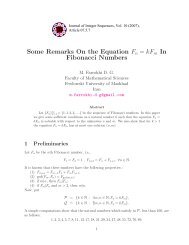
Jiu Zhang Suan Shu and the Gauss Algorithm 11 

Figure 2: Problem 1, Chapter 8 of Jiu Zhang Suan Shu 

The technique given in the chapter for solving these problems is elimination, 

which is exactly the same as the so-called Gauss elimination in the West. For 

example, Problem 1 in the chapter states as follows: 

Problem I. There are three grades of grain: top, medium and low. 

Three sheaves of top-grade, two sheaves of medium-grade and one 

sheaf of low-grade are 39 Dous 4 . Two sheaves of top-grade, three 

sheaves of medium-grade and one sheaf of low-grade are 34 Dous. 

One sheaf of top-grade, two sheaves of medium-grade and three 

sheaves of low-grade are 26 Dous. How many Dous does one sheaf 

of top-grade, medium-grade and low-grade grain yield respectively? 

In the book, the solution is given right after the problem is stated. Afterwards, 

Liu Hui gave a detailed commentary about the algorithm for solving 

the problem. The algorithm described in the book is as follows. 

Putting three sheaves of top-grade grain, two sheaves of mediumgrade 

grain, and one sheaf of low-grade grain and the total 39 Dous 

in a column on the right, then putting the other two columns in the 

middle and on the left. 

4 Dou, a unit of dry measurement for grain in ancient China, is one deciliter. 



This gives the following array: 

1 2 3 

2 3 2 

3 1 1 

26 34 39 

Then, the algorithm continues as follows. 

Multiplying the middle column by top-grade grain of the right column, 

then eliminating top-grade grain from the middle column by 

repeated subtracting the right column. 

This gives the following tabular: 

1 2×3 3 

2 3×3 2 

3 1×3 1 

26 34×3 39 

=⇒ 

1 6−3−3 3 

2 9−2−2 2 

3 3−1−1 1 

26 102−39−39 39 

=⇒ 

1 3 

2 5 2 

3 1 1 

26 24 39 

From the above tabular, we can see that the top position in the middle column 

is already eliminated. Calculations in ancient China were done by moving 

small wood or bamboo sticks (actually, the Chinese translation of operational 

research is Yun Chou which means moving sticks), namely addition is done by 

adding sticks, and subtraction is done by taking away sticks. Thus, when no 

sticks are left in a position (indicating a zero element), this place is eliminated. 

The algorithm goes on as follows. 

Similarly, multiplying the right column and also doing the subtraction. 

The above sentence yields the following tabular: 

1×3−3 3 

2×3−2 5 2 

3×3−1 1 1 

26×3−39 24 39 

=⇒ 

3 

4 5 2 

8 1 1 

39 24 39 

Then, multiplying the left column by medium-grade grain of the middle 

column, and carrying out the repeated subtraction. 

3 

4×5−5×4 5 2 

8×5−1×4 1 1 

39×5−24×4 24 39 

=⇒ 

3 

5 2 

36 1 1 

99 24 39 

Now the remaining two numbers in the left column decides the yield 

of low-grade grain: the upper one is the denominator, the lower one 

is the numerator. 


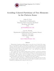
Jiu Zhang Suan Shu and the Gauss Algorithm 13 

Figure 3: Algorithm descriptions, Chapter 8 of Jiu Zhang Suan Shu 

Thus, the yield of low-grade grain = 99/36 = 23 4 Dous. The algorithm continues 

as follows. 

Now, to obtain the yield of medium-grade grain from the middle 

column, the denominator is the top number, and the numerator is 

the bottom number minus the middle number times the yield of lowgrade 

grain. 

Therefore, the yield of medium-grade grain = [24−1×2 3 

4 ]/5 = 41 

4 Dous. 

To calculate the yield of top-grade grain by the right column, the 

denominator is the top number, and the numerator is the bottom 

number minus the second number times the yield of medium-grade 

grain and the third number times the yield of low-grade grain. 

Consequently, the yield of top-grade grain = [39 − 2 × 41 4 − 1 × 23 

4 ]/3 = 91 

4 

Dous. 

It is easy to see that the above procedure is exactly the same as the Gauss 

elimination [2] for the following linear equations: 

3x+2y +z = 39 

2x+3y +z = 34 

x+2y +3z = 26 



The only difference is the way in which the numbers are arranged in the arrays. 

To be more exact, if we rotate all the above rectangular arrays anti-clockwise 

90 degree, we obtain the corresponding matrices of the Gauss elimination. This 

is not unexpected, as in ancient China, people wrote from top to bottom, and 

then from right to left, while in the West, people write from left to right and 

then from top to bottom. 

Thus, from the algorithm description in Chapter 8 of The Nine Chapters on 

the Mathematical Art, we conclude that the Gauss elimination was discovered 

at least over 2200 years ago in ancient China. Recently, more and more western 

scholars [1, 6] credit this simple yet elegant elimination algorithm to ancient 

Chinese mathematicians. For detailed history of the Gauss elimination, there 

are two very good review papers [3, 4], where many interesting stories are told. 

Acknowledgement. I would like to my colleague, Professor Wenlin Li for 

providing all the pictures used in this article. 

References 

[1] P. Gabriel, Matrizen Geometrie Lineare Algebra, Birkhäuser, 1997. 

[2] G.H. Golub and C.F. Van Loan, Matrix Computations (3rd ed.), Johns 

Hopkins, 1996. 

[3] J.F. Grcar, How ordinary elimination became Gaussian elimination, Historia 

Mathematica 38:(2), 163–218, 2011. 

[4] J.F. Grcar, Mathematicians of Gaussian elimination, Notices of the American 

Mathematical Society, 58:(6), 782–792, 2011. 

[5] H. Liu, Jiu Zhang Suan Shu Zhu, (in Chinese), 263. 

[6] C.D. Meyer, Matrix Analysis and Applied Linear Algebra, SIAM, 2000. 

Ya-xiang Yuan 

Academy of Mathematics 

and Systems Science 

Chinese Academy of Sciences 

Zhong Guan Cun Donglu 55 

Beijing 100190 

China 

yyx@lsec.cc.ac.cn 



Leibniz and the Brachistochrone 


2010 Mathematics Subject Classification: 01A45, 49-03 

Keywords and Phrases: Leibniz, Johann Bernoulli, Galileo, cycloid, 

calculus squabble 

1696 was the year of birth of the calculus of variations. As usual in those days, 

the Swiss mathematician Johann Bernoulli, one of Leibniz’s closest friends 

and followers, issued a provocative mathematical challenge in the scholarly 

journal Acta Eruditorum (Transactions of scholars) in June 1696 inviting the 

mathematicians to solve this new problem: 

Given two points A and B in a vertical plane, find the path AMB 

down which a movable point M must by virtue of its weight fall from 

A to B in the shortest possible time. 

In order to encourage “the enthusiasts of such things” (harum rerum amatores) 

Bernoulli emphasized the usefulness of the problem not only in mechanics but 

also in other sciences and added that the curve being sought is not the straight 

line but a curve well-known to geometers. He would publicize it by the end 

of the year if nobody should publicize it within this period. When Bernoulli 

published his challenge he did not know that Galileo had dealt with a related 

problem without having in mind Bernoulli’s generality. And he could not know 

that his challenge would lead to one of the most famous priority disputes in 

the history of mathematics. 

He communicated the problem to Leibniz in a private letter, dated June 

19, 1696 and dispatched from Groningen in the Netherlands, asking him to 

occupy himself with it. Leibniz sent him his answer, together with the correct 

solution, just one week later on June 26 from Hannover. He proposed the 

name tachystoptota (curve of quickest descent), avowing that the problem is 

indeed most beautiful and that it had attracted him against his will and that 

he hesitated because of its beauty like Eve before the apple. He deduced 

the correct differential equation but failed to recognize that the curve was a 

cycloid until Bernoulli informed him in his answer dating from July 31. He 

took up Leibniz’s biblical reference adding that he was very happy about this 

comparison provided that he was not regarded as the snake that had offered 

the apple. Leibniz must certainly have been happy to hear that the curve is the 


16 Eberhard Knobloch 

Figure 1: Bernoulli’s figure of the brachistochrone (Die Streitschriften von 

Jacob und Johann Bernoulli, Variationsrechnung. Bearbeitet und kommentiert 

vonHermanH.Goldstine, mithistorischenAnmerkungenvonPatriciaRadeletde 

Grave. Basel-Boston-Berlin 1991, 212) 

cycloid, for which Huygens had shown the property of isochronism. For that 

reason he, Bernoulli, had given it the name brachystochrona. Leibniz adopted 

Bernoulli’s description. 

On June 28 he had already communicated the problem to Rudolf Christian 

von Bodenhausen in Florence, again praising its extraordinary beauty in order 

to encourage the Italian mathematicians to solve it. In Switzerland Jacob 

Bernoulli, and in France Pierre Varignon, had been informed. He asked Johann 

Bernoulli to extend the deadline until June 1697 because in late autumn 1696 

the existence of only three solutions, by Johann and his elder brother Jacob 

Bernoulli and by himself, were known. Bernoulli agreed insofar as he published 

a new announcement in the December issue of the Acta Eruditorum that he 

would suppress his own solution until Easter 1697. In addition to that he wrote 

a printed leaflet that appeared in January 1697. 

The May 1697 issue of the Acta Eruditorum contained an introductory historical 

paper by Leibniz on the catenary and on the brachistochrone. He renounced 

the publication of his own solution of the brachistochrone problem 

because it corresponded, he said, with the other solutions (cum caeteris consentiat). 

Then the five known solutions by Johann, Jacob Bernoulli, the Marquis 

de l’Hospital, Ehrenfried Walther von Tschirnhaus, and Isaac Newton were 

published or reprinted (Newton). Newton had not revealed his name. But 

Johann Bernoulli recognized the author, “from the claw of the lion” (ex ungue 

leonem), as he said. 


Leibniz and the Brachistochrone 17 

Figure2: Galileo’sfigureregardingthefallofaparticlealongacircularpolygon 

(Galileo Galilei: Le opere, vol. VIII, Firenze 1965, 262) 

Leibniz made some statements in his paper that are worth discussing. First 

of all he maintained that Galileo had already dealt with the catenary and with 

the brachistochrone as well, without being able to find the correct solution. 

He had falsely identified the catenary with a parabola and the brachistochrone 

with a circular arc. Unfortunately Johann Bernoulli relied on Leibniz’s false 

statement and repeated it in June 1697, and later so did many other authors up 

to the present time. Neither the one nor the other assertion is in reality true. 

What had Galileo really said in his Discorsi? He had rightly emphasized the 

similarity between the catenary and a parabola. He did not and could not look 

forthecurveofquickestdescent, thatis, forthebrachistochrone. Suchageneral 

problem was still beyond the mathematical horizon of the mathematicians of 

his time. 

He had considered an arc of a circle CBD of not more than 90° in a vertical 

plane with C the lowest point on the circle, D the highest point and B any 

other point on the arc of the circle. He proved the correct theorem that the 

time for a particle to fall along the broken line DBC is less than the time for 

it to descend along the line DC. Let us enlarge the number of points on the 

circle between D and C. The larger the number of points is, the less is the 

time for the particle to descend along the broken line DEFG...C. For Galileo 

a circle was a polygon with infinitely many, infinitely small sides. Hence he 

rightly concluded that the swiftest time of fall from D to C is along a portion 

of the circle. Galileo only compared the times of fall along the sides of circular 

polygons the circle being the limit case of them. 

Secondly, Leibniz said that the only mathematicians to have solved the problem 

are those he had guessed would be capable of solving it; in other words, 



only those who had suffiently penetrated in the mysteries of his differential 

calculus. This he had predicted for the brother of Johann Bernoulli and the 

Marquis de l’Hospital, for Huygens if he were alive, for Hudde if he had not 

given up such pursuits, for Newton if he would take the trouble. The words 

were carelessly written because their obvious meaning was that Newton was 

indebted to the differential calculus for his solution. Even if Leibniz did not 

want to make such a claim, and this is certain in 1697, his words could be 

interpreted in such a way. There was indeed a reader who chose this interpretation: 

the French emigrant Nicolas Fatio de Duillier, one of Newton’s closest 

followers. Fatio was deeply offended at not having been mentioned by Leibniz 

among those authors who could master the brachistochrone problem. In 1699 

he published a lengthy analysis of the brachistochrone. Therein he praised his 

own mathematical originality and sharply accused Leibniz of being only the 

second inventor of the calculus. Fatio’s publication was the beginning of the 

calculus squabble. But this is another story. 

References 

[1] H.H.Goldstine, Introduction, in: DieStreitschriftenvonJacobundJohann 

Bernoulli, Variationsrechnung, bearbeitetundkommentiertvonH.H.Goldstine 

mit historischen Anmerkungen von P. Radelet-de Grave, Birkhäuser, 

Basel-Boston-Berlin 1991, pp. 1–113. 

[2] E. Knobloch, Le calcul leibnizien dans la correspondance entre Leibniz et 

Jean Bernoulli. in: G. Abel, H.-J. Engfer, C. Hubig (eds.), Neuzeitliches 

Denken, Festschrift für Hans Poser zum 65. Geburtstag, W. de Gruyter, 

Berlin-New York 2002, pp. 173–193. 

[3] Eberhard Knobloch, Galilei und Leibniz, Wehrhahn, Hannover 2012. 

[4] Jeanne Peiffer, Le problème de la brachystochrone à travers les relations 

de Jean I. Bernoulli avec l’Hospital et Varignon, in: H.-J. Hess, F. Nagel 

(eds.), Der Ausbau des Calculus durch Leibniz und die Brüder Bernoulli. 

Steiner, Wiesbaden 1989, pp. 59–81 (= Studia Leibnitiana Sonderheft 17). 


Berlin-Brandenburg Academy 

of Sciences and Humanities 

Technische Universität Berlin 

H 72 

Straße des 17. Juni 135 

10623 Berlin 

eberhard.knobloch@tu-berlin.de 



Leibniz and the Infinite 



Keywords and Phrases: Leibniz, infinite, infinitely small, mathematical 

rigour, integration theory 

TheGermanuniversal genius Gottfried Wilhelm Leibnizwas bornin Leipzigon 

the 21st of June according to the Julian calendar (on the 1st of July according 

to the Gregorian calendar) 1646. From 1661 he studied at the universities of 

Leipzig and Jena. On February 22, 1667 he became Doctor of Laws at the 

university of Nürnberg-Altdorf. He declined the professorship that was offered 

to him at this university. For a short time he accepted a position at the court 

of appeal of Mainz. From 1672 to 1676 he spent four years in Paris where he 

invented his differential and integral calculus in autumn 1675. 

From1676uptotheendofhislifeheearnedhislivingaslibrarianatthecourt 

of the duke, then elector, of Hannover. In 1700 he was appointed president of 

the newly founded Electoral Academy of Sciences of Berlin. He contributed 

to nearly all scientific disciplines and left the incredibly huge amount of about 

200 000 sheets of paper. Less than one half of them have been published up to 

now. 

In Paris he became one of the best mathematicians of his time within a few 

years. He was especially interested in the infinite. But what did he mean 

by this notion? His comments on Galileo’s Discorsi give the answer. Therein 

Galileo had demonstrated that there is a one-to-one correspondence between 

the set of the natural numbers and the set of the square numbers. Hence in his 

eyes the Euclidean axiom “The whole is greater than a part” was invalidated in 

the sense that it could not be applied there: infinite sets cannot be compared 

with each other with regard to their size. Leibniz contradicted him. For him it 

was impossible that this axiom failed. This only seemed to be the case because 

Galileo had presupposed the existence of actually infinite sets. For him the 

universal validity of rules was more important than the existence of objects, in 

this case of actually infinite numbers or actually infinite sets. Hence Leibniz 

did not admit actual infinity in mathematics. “Infinite” meant “larger than 

any given quantity”. He used the mode of possibility in order to characterize 

the mathematical infinite: it is always possible to find a quantity that is larger 

than any given quantity. 



Figure 1: Portrait of Leibniz by A. Scheit, 1703 (By courtesy of the Gottfried 

Wilhelm Leibniz Library, Hannover) 

By using the mode of possibility he consciously imitated ancient models 

like Aristotle, Archimedes, and Euclid. Aristotle had defined the notion of 

quantity in his Metaphysics: quantity is what can be divided into parts being 

in it. Something (a division) can be done in this case. If a division of a certain 

object is not possible, the object cannot be a quantity. In the 17th and 18th 

centuries mathematics was the science of quantities. Hence it could not handle 

non-quantities. Hence Leibniz avoided non-quantities in mathematics by all 

means. 

Indivisibles were non-quantities by definition: they cannot be divided. Yet 

they occurred even in the title of Bonaventura Cavalieri’s main work Geometry 

developedbyanewmethodbymeansoftheindivisibles ofcontinua. Cavalieri’s 

indivisibles were points of a line, straight lines of a plane, planes of a solid. 

Leibniz amply used this notion, for example in the title of the first publication 

of his integral calculus Analysis of indivisibles and infinites that appeared in 

1686. But according to his mathematical convictions he had to look for a 

suitable, new interpretation of the notion. 

From 1673 he tried different possibilities like smallest, unassignable magnitude, 

smaller than any assignable quantity. He rightly rejected all of them 

because there are no smallest quantities and because a quantity that is smaller 

than any assignable quantity is equal to zero or nothing. In spring 1673 he 


Leibniz and the Infinite 21 

finally stated that indivisibles have to be defined as infinitely small quantities 

or the ratio of which to a perceivable quantity is infinite. Thus he had shifted 

the problem. Now he had to answer the question: What does it mean to be infinitely 

small? Still in 1673 he gave an excellent answer: infinitely small means 

smaller than any given quantity. He again used the mode of possibility and 

introduced a consistent notion. Its if-then structure – if somebody proposes a 

quantity, then there will be a smaller quantity – rightly reminds the modern 

reader of Weierstraß’s ǫ-δ-language. Leibniz’s language can be translated into 

Weierstraß’s language. 

Leibniz used this well-defined notion throughout the longest mathematical 

treatiseheeverwrote, inhisArithmeticalquadratureofthecircle, oftheellipse, 

and of the hyperbola. Unfortunately it remained unpublished during his lifetime 

though he wrote it already in the years 1675/76. Only in 1993 did the 

first printed version appear in Göttingen. 

For this reason Leibniz has been falsely accused of neglecting mathematical 

rigour again and again up to the present day. His Arithmetical quadrature 

contains the counterdemonstration of that false criticism. Therein theorem 6 

gives a completely rigorous foundation of infinitesimal geometry by means of 

Riemannian sums. Leibniz foresaw its deterrent effect saying: 

Thereadingofthispropositioncanbeomittedifsomebodydoesnot 

want supreme rigour in demonstrating proposition 7. And it will be 

better that it be disregarded at the beginning and that it be read 

only after the whole subject has been understood, in order that its 

excessiveexactnessdoesnotdiscouragethemindfromtheother, far 

moreagreeable, thingsbymakingitbecomewearyprematurely. For 

it achieves only this: that two spaces of which one passes into the 

other if we progress infinitely, approach each other with a difference 

that is smaller than any arbitrary assigned difference, even if the 

number of steps remains finite. This is usually taken for granted, 

even by those who claim to give rigorous demonstrations. 

Leibniz referred to the ancients like Archimedes who was still the model of 

mathematical rigour. After the demonstration Leibniz stated: “Hence the 

method of indivisibles which finds the areas of spaces by means of sums of lines 

can be regarded as proven.” He explicitly formulated the fundamental idea of 

the differential calculus, that is, the linearization of curves: 

The readers will notice what a large field of discovery is opened up 

once they have well understood only this: that every curvilinear 

figure is nothing but a polygon with infinitely many infinitely small 

sides. 

Whenhepublishedhisdifferentialcalculusforthefirsttimein1684herepeated 

this crucial idea. From that publication he had to justify his invention. In 1701 

he rightly explained: 



Figure 2: First page of Leibniz’s treatise Arithmetical quadrature of the circle 

etc. (By courtesy of the Gottfried Wilhelm Leibniz Library, Hannover. Shelf 

mark LH XXXV 2,1 folio 7r) 


Leibniz and the Infinite 23 

Because instead of the infinite and the infinitely small one takes 

quantities that are as large or as small as it is necessary so that the 

error is smaller than the given error so that one differs from the 

style of Archimedes only by the expressions which are more direct 

in our method and more suitable for the art of invention. 

The story convincingly demonstrates the correctness of his saying: “Those who 

know me only by my publications don’t know me.” 

References 

[1] E. Knobloch, Leibniz’s rigorous foundation of infinitesimal geometry by 

means of Riemannian sums, Synthese 133 (2002), 59–73. 

[2] [2] E. Knobloch, Galileo and German thinkers: Leibniz, in: L. Pepe (ed.), 

Galileo e la scuola galileiana nelle Università del Seicento, Cooperativa Libraria 

Universitaria Bologna, Bologna 2011, pp. 127–139. 





H 72 


10623 Berlin 



24 



A Short History of Newton’s Method 


2010 Mathematics Subject Classification: 01A45, 65-03, 65H05, 

65H10, 65J15, 65K99 

Keywords and Phrases: History of Newton’s method, Simpson, Raphson, 

Kantorovich, Mysoskikh, geometric approach, algebraic approach 

If an algorithm converges unreasonably fast, 

it must be Newton’s method. 

John Dennis (private communication) 

It is an old dream in the design of optimization algorithms, to mimic Newton’s 

method due to its enticing quadratic convergence. But: Is Newton’s method 

really Newton’s method? 

Linear perturbation approach 

Assume that we have to solve a scalar equation in one variable, say 

f(x) = 0 

with an appropriate guess x 0 of the unknown solution x ∗ at hand. Upon 

introducing the perturbation 

∆x = x ∗ −x 0 , 

Taylor’s expansion dropping terms of order higher than linear in the perturbation, 

yields the approximate equation 

f ′ (x 0 )∆x . = −f(x 0 ) , 

which may lead to an iterative equation of the kind 

x k+1 = x k − f(xk ) 

f ′ (xk , k = 0,1,... 

) 


26 Peter Deuflhard 

assuming the denominator to be non-zero. This is usually named Newton’s 

method. The perturbation theory carries over to rather general nonlinear operator 

equations, say 

F(x) = 0, x ∈ D ⊂ X, F : D → Y, 

where X,Y are Banach spaces. The corresponding Newton iteration is then 

typically written in the form 

F ′ (x k )∆x k = −F(x k ), x k+1 = x k +∆x k , k = 0,1,... 

For more details and extensions see, e.g., the textbook [1] and references 

therein. 

Convergence 

From the linear perturbation approach, local quadratic convergence will be 

clearly expected for the scalar case. For the general case of operator equations 

F(x) = 0, the convergence of the generalized Newton scheme has first 

been proven by two Russian mathematicians: In 1939, L. Kantorovich [5] was 

merely able to show local linear convergence, which he improved in 1948/49 to 

local quadratic convergence, see [6, 7]. Also in 1949, I. Mysovskikh [9] gave a 

much simpler independent proof of local quadratic convergence under slightly 

different theoretical assumptions, which are exploited in modern Newton algorithms, 

see again [1]. Among later convergence theorems the ones due to J. 

Ortega and W.C. Rheinboldt [11] and the affine invariant theorems given in 

[2, 3] may be worth mentioning. 

Geometric approach 

The standard approach to Newton’s method in elementary textbooks is given 

in Figure 1. It starts from the fact that any root of f may be interpreted as the 

intersection of the graph of f(x) with the real axis. In Newton’s method, this 

graph is replaced by its tangent in x0; the first iterate x1 is then defined as the 

intersection of the tangent with the real axis. Upon repeating this geometric 

process, aclose-bysolutionpointx ∗ canbeconstructedtoanydesiredaccuracy. 

On the basis of this geometric approach, this iteration will converge globally 

for convex (or concave) f. 

At first glance, this geometric derivation seems to be restricted to the scalar 

case, since the graph of f(x) is a typically one-dimensional concept. A careful 

examination of the subject in more than one dimension, however, naturally 

leads to a topological path called Newton path, which can be used for the 

construction of modern adaptive Newton algorithms, see again [1]. 


Historical road 

A Short History of Newton’s Method 27 

0 

f(x0) 

f 

x0 

Figure 1: Newton’s method for a scalar equation 

The long way of Newton’s method to become Newton’s method has been well 

studied, see, e.g., N. Kollerstrom [8] or T.J. Ypma [13]. According to these 

articles, the following facts seem to be agreed upon among the experts: 

• In 1600, Francois Vieta (1540–1603) had designed a perturbation technique 

for the solution of the scalar polynomial equations, which supplied 

one decimal place of the unknown solution per step via the explicit calculation 

of successive polynomials of the successive perturbations. In 

modern terms, the method converged linearly. It seems that this method 

had also been published in 1427 by the Persian astronomer and mathematician 

al-Kāshī (1380–1429) in his The Key to Arithmetic based on 

much earlier work by al-Biruni (973–1048); it is not clear to which extent 

this work was known in Europe. Around 1647, Vieta’s method was 

simplified by the English mathematician Oughtred (1574–1660). 

• In 1664, Isaac Newton (1643–1727) got to know Vieta’s method. Up to 

1669 he had improved it by linearizing the successively arising polynomials. 

As an example, he discussed the numerical solution of the cubic 

polynomial 

f(x) := x 3 −2x−5 = 0 . 

Newton first noted that the integer part of the root is 2 setting x0 = 2. 

Next, by means of x = 2+p, he obtained the polynomial equation 

x∗ 

p 3 +6p 2 +10p−1 = 0 . 

He neglected terms higher than first order setting p ≈ 0.1. Next, he 

inserted p = 0.1+q and constructed the polynomial equation 

q 3 +6.3q 2 +11.23q +0.061 = 0 . 

Again neglecting higher order terms he found q ≈ −0.0054. Continuation 

of the process one further step led him to r ≈ 0.00004853 and therefore 

to the third iterate 

x3 = x0 +p+q +r = 2.09455147 . 


x


Note that the relations 10p−1 = 0 and 11.23q +0.061 = 0 given above 

correspond precisely to 

and to 

p = x1 −x0 = −f(x0)/f ′ (x0) 

q = x2 −x1 = −f(x1)/f ′ (x1) . 

As the example shows, he had also observed that by keeping all decimal 

places of the corrections, the number of accurate places would double per 

each step – i.e., quadratic convergence. In 1687 (Philosophiae Naturalis 

Principia Mathematica), the first nonpolynomial equation showed up: it 

is the well-known equation from astronomy 

x−esin(x) = M 

betweenthemean anomaly M andtheeccentric anomaly x. HereNewton 

usedhisalreadydevelopedpolynomialtechniquesviatheseriesexpansion 

ofsin andcos. However, nohintonthederivativeconceptisincorporated! 

• In 1690, Joseph Raphson (1648–1715) managed to avoid the tedious computation 

ofthesuccessivepolynomials, playingthecomputational scheme 

back to the original polynomial; in this now fully iterative scheme, he 

also kept all decimal places of the corrections. He had the feeling that 

his method differed from Newton’s method at least by its derivation. 

• In 1740, Thomas Simpson (1710–1761) actually introduced derivatives 

(‘fluxiones’)inhisbook‘EssaysonSeveralCuriousandUsefulSubjectsin 

Speculative and Mix’d Mathematicks [No typo!], Illustrated by a Variety 

of Examples’. He wrote down the true iteration for one (nonpolynomial) 

equation and for a system of two equations in two unknowns thus making 

the correct extension to systems for the first time. His notation is already 

quite close to our present one (which seems to date back to J. Fourier). 

The interested reader may find more historical details in the book by H. H. 

Goldstine [4] or even try to read the original work by Newton in Latin [10]; 

however, even with good knowledge of Latin, this treatise is not readable to 

modern mathematicians due to the ancient notation. That is why D.T. Whiteside 

[12] edited a modernized English translation. 

What is Newton’s method? 

Under the aspect of historical truth, the following would come out: 

• For scalar equations, one might speak of the Newton–Raphson method. 

• For more general equations, the name Newton–Simpson method would 

be more appropriate. 


A Short History of Newton’s Method 29 

Under the convergence aspect, one might be tempted to define Newton’s 

method via its quadratic convergence. However, this only covers the pure Newton 

method. There are plenty of variants like the simplified Newton method, 

Newton-like methods, quasi-Newton methods, inexact Newton methods, global 

Newton methods etc. Only very few of them exhibit quadratic convergence. 

In fact, even the Newton–Raphson algorithm for scalar equations as realized 

in hardware within modern calculators converges only linearly due to finite 

precision, which means they asymptotically implement some Vieta algorithm. 

Hence, one will resort to the fact that Newton methods simply exploit derivative 

information in one way or the other. 

Acknowledgement 

The author wishes to thank E. Knobloch for having pointed him to several 

interesting historical sources. 

References 

[1] P. Deuflhard. Newton Methods for Nonlinear Problems. Affine Invariance 

and Adaptive Algorithms, volume 35 of Computational Mathematics. 

Springer International, 2004. 

[2] P. Deuflhard and G. Heindl. Affine Invariant Convergence theorems for 

Newton’s Method and Extensions to related Methods. SIAM J. Numer. 

Anal., 16:1–10, 1979. 

[3] P. Deuflhard and F.A. Potra. Asymptotic Mesh Independence of Newton- 

Galerkin Methods via a Refined Mysovskii Theorem. SIAM J. Numer. 

Anal., 29:1395–1412, 1992. 

[4] H. H. Goldstine. A history of Numerical Analysis from the 16th through 

the 19th Century. Spri9nger, 1977. 

[5] L. Kantorovich. The method of successive approximations for functional 

equations. Acta Math., 71:63–97, 1939. 

[6] L.Kantorovich. OnNewton’sMethodforFunctionalEquations.(Russian). 

Dokl. Akad. Nauk SSSR, 59:1237–1249, 1948. 

[7] L. Kantorovich. On Newton’s Method. (Russian). Trudy Mat. Inst. 

Steklov, 28:104–144, 1949. 

[8] N. Kollerstrom. Thomas Simpson and ‘Newton’s Method of Approximation’: 

an enduring myth. British Journal for History of Science, 25:347– 

354, 1992. 

[9] I. Mysovskikh. On convergence of Newton’s method. (Russian). Trudy 

Mat. Inst. Steklov, 28:145–147, 1949. 



[10] I. Newton. Philosophiae naturalis principia mathematica. Colonia Allobrogum: 

sumptibus Cl. et Ant. Philibert, 1760. 

[11] J.M. Ortega and W.C. Rheinboldt. Iterative Solution of Nonlinear Equations 

in Several Variables. Classics in Appl. Math. SIAM Publications, 

Philadelphia, 2nd edition, 2000. 

[12] D.T. Whiteside. The Mathematical Papers of Isaac Newton (7 volumes), 

1967–1976. 

[13] T.J. Ypma. Historical Development of the Newton-Raphson Method. 

SIAM Rev., 37:531–551, 1995. 


Konrad-Zuse-Zentrum 

für Informationstechnik 

Berlin (ZIB) 

Takustraße 7 

14195 Berlin 

Germany 

deuflhard@zib.de 



Euler and Infinite Speed 



Keywords and Phrases: Euler, Galileo, Maupertuis, tunnel through 

the earth, damped oscillation 

ThefamousSwissmathematicianLeonhardEulerwasborninBaselonthe15th 

of April 1707. Already in 1720 when he was still a thirteen-year-old boy, he 

enrolled at the University of Basel. One year later, he obtained the Bachelor’s 

degree. In 1723 when he was sixteen years old, he obtained his Master’s degree 

(A. L. M. = Master of Liberal Arts). 

In 1727 without ever having obtained the Ph. D. degree he submitted a short 

habilitation thesis (consisting of fifteen pages); that is, a thesis in application 

for the vacant professorship of physics at the University of Basel. At that time 

he had published two papers, one of them being partially faulty. No wonder 

that the commission which looked for a suitable candidate for the professorship 

did not elect him. Yet Euler was very much infuriated by this decision. Still 

in 1727, he went to St. Petersburg in order to work at the newly founded 

Academy of Sciences. He never came back to Switzerland. Between 1741 and 

1766 he lived and worked in Berlin at the reformed Academy of Sciences and 

Literature of Berlin. In 1766 he returned to St. Petersburg where he died on 

the 18th of September 1783. 

The complete title of his habilitation thesis reads: 

May it bring you happiness and good fortune – Physical dissertation 

on sound which Leonhard Euler, Master of the liberal arts submits 

to the public examination of the learned in the juridical lecture-room 

on February 18, 1727 at 9 o’clock looking at the free professorship 

of physics by order of the magnificent and wisest class of philosophers 

whereby the divine will is nodding assent. The most eminent 

young man Ernst Ludwig Burchard, candidate of philosophy, is responding. 

As we know, all imploring was in vain: Euler did not get the position. The 

thesisisallthemoreinterestingbecauseEulerhadaddedasupplementinwhich 

he formulated six statements regarding utterly different subjects. For example 

he maintained that Leibniz’s theory of preestablished harmony between body 



Figure 1: Leonhard Euler (1707–1783) (L. Euler, Opera omnia, series I, vol. 1, 

Leipzig – Berlin 1911, Engraving after p. I) 

and soul is false, without mentioning the name of his illustrious predecessor. 

Another statement prescribed the construction of a ship mast. 

The third statement considered a thought experiment: What would happen 

at the centre of the earth if a stone were dropped into a straight tunnel drilled 

to the centre of the earth and beyond to the other side of the planet? 

Euler distinguished between exactly three possiblities: Either the stone will 

rest at the centre or will at once proceed beyond it or it will immediately return 

from the centre to us. There is no mention of speed. Euler just stated that 

the last case will take place. No justification or explanation is given, though 

none of these three possibilities had the slightest evidence. What is worse, a 

far better answer had been already given by Galileo in 1632. 

In the second day of his Dialogue about the two main world systems Galileo 

discussed this thought experiment in order to refute Aristotle’s distinction between 

natural and unnatural motions. The natural motion of heavy bodies 

is the straight fall to the centre of the earth. But what about a cannon ball 


Euler and Infinite Speed 33 

Figure 2: Title page of Euler’s Physical dissertation on sound (L. Euler, Opera 

omnia, series III, vol. 1, Leipzig – Berlin 1926, p. 181) 

that has dropped into such an earth tunnel? Even the Aristotelian Simplicio 

avowed that the cannon ball would reach the same height from which it had 

dropped into the tunnel in the other half of the tunnel. The natural motion 

would change into an unnatural motion. 

Galileo erroneously presupposed a constant gravitation. But he rightly deduced 

an oscillating motion of the cannon ball. Euler did not mention the Italian 

mathematician. Presumably he did not know his solution of the thought 

experiment. Nine years later he came back to this question in his Mechanics or 

the science of motion set forth analytically. Now he explicitly concluded that 

the speed of the falling stone will become infinitely large in the centre of the 

earth. Nevertheless it will immediately return to the starting-point. 

Euler admitted: 

This seems to differ from truth because hardly any reason is obvious 

why a body, having infinitely large speed that it has acquired in C, 

should proceed to any other region than to CB, especially because 

the direction of the infinite speed turns to this region. However 

that may be, here we have to be confídent more in the calculation 

than in our judgement and to confess that we do not understand at 

all the jump if it is done from the infinite into the finite. 



Figure 3: L. Euler, Mechanics, vol. 1, 1736, § 272 (Explanation 2) (L. Euler, 

Opera omnia, series II, vol. 1, Leipzig – Berlin 1912, p. 88) 

Euler’s result was the consequence of his mathematical modelling of the situation 

(an impermissible commutation of limits). When in 1739 Benjamin 

Robbins wrote his review of Euler’s Mechanics he put as follows: 

When y, the distance of the body from the center, is made negative, 

the terms of the distance expressedbyy n , wherenmay beany number 

affirmative, or negative, whole number or fraction, are sometimes 

changed with it. The centripetal force being as some power of 

the fraction; if, when y is supposed negative, y n be still affirmative, 

the solution gives the velocity of the body in its subsequent ascent 

from the center; but if y n by this supposition becomes also negative, 

the solution exhibits the velocity, after the body has passed 

the center, upon condition, that the centripetal force becomes centrifugal; 

and when on this supposition y n becomes impossible, the 

determination of the velocity beyond the center is impossible, the 

condition being so. 

The French physicist Pierre-Louis Moreau de Maupertuis was the president of 

the Academy of Sciences and of Literature in Berlin at the beginning of Euler’s 

sojourninBerlin. Heunfortunatelyproposedtoconstructsuchanearthtunnel. 

His proposal was ridiculed by Voltaire on the occasion of the famous quarrel 

about theprinciple of least action between Maupertuis, Euler, andthe Prussian 

king Frederick the Great on the one side and the Swiss mathematician Samuel 

König on the other side. Thus Euler’s curious statement about the dropping 

stone had a satirical aftermath. In 1753 Voltaire published his Lampoon of 


Euler and Infinite Speed 35 

Doctor Akakia. Therein he made Euler regret that he had more confídence in 

his calculation than in human judgement. In truth Euler never recanted his 

solution. 

References 

[1] Emil A. Fellmann: Leonhard Euler, translated by Erika Gautschi and Walter 

Gautschi. Basel – Boston – Berlin 2007. 

[2] Eberhard Knobloch: Euler – The historical perspective. In: Physica D 237 

(2008), 1887–1893. 

[3] Rüdiger Thiele: Leonhard Euler. Leipzig 1982. 





H 72 


10623 Berlin 



36 



Euler and Variations 


2010 Mathematics Subject Classification: 01A50, 01A70 

Keywords and Phrases: Euler, Seven-Years War, Euler’s estate in 

Lietzow, Euler’s losses 

When Euler came to Berlin in 1741, accepting the offer of the Prussian king 

Frederick II. to work at the Berlin academy of sciences, the king himself was 

at the first Silesian war with Austria. It was only the first of three wars that 

he waged. Two years later Euler bought a house in the centre of Berlin in the 

“Bärenstraße”, today “Behrenstraße” number 21. There he lived up to 1766 

when he left Berlin in order to return to St. Petersburg. 

Yet already in those days, life was expensive in a city like Berlin. Hence 

in 1753 he bought an estate outside Berlin in the small village of Lietzow, 

belonging to the administrative district of Charlottenburg, that is to-day a part 

of a district of the city of Berlin. He paid 6000 Imperial Taler (Reichsthaler) 

for it. From then onward his large family lived on this estate, including his 

widowed mother, while he himself remained in Berlin. 

WheneverhehadRussianstudentsofmathematicstheytoolivedinthehouse 

in Berlin: from 1743 to 1744 Kirill Grigorevich Rasumovskii, later president 

of the Russian Academy of Sciences in St. Petersburg, and Grigorii Nikolaevich 

Teplov, from 1752 to 1756 Semen Kirillovich Kotelnikov, in 1754 Michail 

Sofronov, from 1754 to 1756 Stepan Yakovlevich Rumovskii. It did not happen 

by chance that 1756 was the year of departure. In 1756 Frederick II. began 

the Seven-Years War by penetrating into Saxony. His Prussian troops fought 

against the allied Russian, Saxon, and Austrian troops. 

Euler carried on sending scientific manuscripts to St. Petersburg – that 

is, to Russia – and kept his good relations with the academy there. Yet he 

secretly helped the Prussian king with his knowledge of the Russian language 

by translating intercepted Russian messages. If the time did not suffice for 

a diligent translation he offered to summarize the content. For example in 

September 1758 a courier of the Russian guard was taken captive together 

with two Cossacks near to Neustettin. They carried seventy-nine letters for the 

Russian court. Euler’s translation of the report of a Russian agent and of the 

statements of two Prussian deserters is still kept in the archives of the Berlin- 

Brandenburg Academy of Sciences and Humanities (http://euler.bbaw.de/ 

euleriana/ansicht.php?seite=216). 



The following years became very difficult for the Prussian king. In 1759 the 

allied Austrian and Russian troops defeated the troops of Frederick II. in the 

neighbourhood of Kunersdorf. On October 9, 1760 Russian and Saxon troops 

temporarily occupied Berlin and plundered the surrounding villages, especially 

Lietzow, and including Euler’s estate. The command of the Russian Count 

Chernishef to spare this estate from plunder came too late. 

Just nine days later, on October 18, 1760 Euler wrote to the historian Gerhard 

Friedrich Müller in St. Petersburg, since 1754 perpetual secretary of the 

Russian Academy of Sciences, in order to complain about this robbery and 

to make a claim for damages. “I have always wished that Berlin should be 

occupied by Russian troops if it should be ever occupied by foreign troops”, 

he wrote, “yet the visit of the Russian officers entailed considerable damage.” 

He told Müller that he had bought an estate for 6000 Imperial Taler in Charlottenburg 

that was well-known to Mr. Kotelnikov and to Mr. Rumovskii. 

On the occasion of that visit everything was removed or devastated. Then he 

enumerated the losses: 

I have lost four horses, twelve cows, many head of livestock, much 

oats and hay. All of the furniture of the house has been ruined. 

This damage is more than 1100 Imperial Taler according to an 

exact calculation...All in all the damage is at least 1200 roubles. 

He asked Müller to inform his former student, then president of the Russian 

Academy, Count Rasumovskii, about his situation and to support his request. 

He was indeed amply recompensed by the Russian general and by the Russian 

tsarina Elisabeth. 

By chance Euler’s statements about his losses can be checked because the 

mayor of Charlottenburg elaborated a specification of damages for Lietzow and 

Charlottenburg that has been preserved in the Main Archives of the country 

Brandenburg of the Federal Republic of Germany in Potsdam. On October 24, 

1760, the mayor sent a letter to the responsible Privy Councillor of War and 

of Domain (Geheimder Krieges und Domainen Rath) saying: 

As we have been ordered we have added and would like to most 

obediently submit the specification of money, grain, and cattle that 

the city of Charlottenburg has lost by the Russian invasion. 

[Anbefohlener Maßen haben Wir angeschlossen die Specification so 

wohlanbaarenGeldealsanGetreydeundViehwasdieStadtCharlottenburg 

durch die Russischen Invasion verlohren haben gehorsamst 

einreichen sollen.] 

The list consists of nine columns. They enumerate the names of the twelve 

families concerned from the village of Lietzow and the robbery of cash currency, 

rye, barleyandoat, hay, horses, cows, pigs, andsheep. Thefourthlinementions 

Euler’s losses reading: 


Euler and Variations 39 

Figure 1: Letter of the mayor of Charlottenburg dating from October 24, 1760 

(By courtesy of the Brandenburgisches Landeshauptarchiv Potsdam, Rep. 2 

Kurmärkische Kriegs- und Domänenkammer Nr. S 3498) 

ProfessorEuler: nocashcurrency; 1Wispel, 5Scheffelrye(1Wispel 

= 24 Scheffel, 1 Scheffel = 54,73 litres); 1 Wispel, 6 Scheffel barley 

andoat; 30metrichundred-weightofhay; twohorses; thirteencows; 

seven pigs; twelve sheep. 



Figure 2: List of damages regarding the village Lietzow (By courtesy of the 

Brandenburgisches Landeshauptarchiv Potsdam, Rep. 2 Kurmärlische Kriegsund 

Domänenkammer Nr. S 3498) 

The astonished reader notices at once that Euler has doubled the number of 

stolen horses. In 1763 he had already negotiated with the Russian Academy 

of Sciences for his return to St. Petersburg, which indeed took place in 1766. 

For that reason he sold his estate in Charlottenburg for 8500 Imperial Taler, 

that is, at a profit of more than forty per cent, thus practising again his private 

calculus of variations. All in all he made a good profit out of his estate. 


Euler and Variations 41 

Figure 3: Title page of Euler’s book on the calculus of variations (L. Euler, 

Opera omnia, series I, vol. 24, Bern 1952, p. 1) 

Thanks to a letter from Euler to the president Maupertuis of the Berlin 

Academy of Sciences and Fine Arts from March 14, 1746 we know that Euler 

had written his official, famous book on the calculus of variations, his Method 

of finding curves with an extreme property or the solution of the isoperimetric 

problem understood in the broadest sense, already in St. Petersburg, that is, 

in spring 1741 at the latest. It appeared in Lausanne in 1744 including the 

appendixIIwithEuler’sexplanationoftheprincipleofleastaction. Constantin 

Carathéodory called the book one of the most beautiful mathematical works 

that has ever been written. But that is another story. 



References 

[1] EberhardKnobloch: LeonhardEuler1707–1783, Zum300.Geburtstageines 

langjährigen Wahlberliners. In: Mitteilungen der Deutschen Mathematiker- 

Vereinigung 15 (2007), 276–288. 





H 72 


10623 Berlin 




Euler, Mei-Ko Kwan, Königsberg, 

and a Chinese Postman 

Martin Grötschel and Ya-xiang Yuan 

2010 Mathematics Subject Classification: 00-02, 01A05, 05C38, 90-03 

Keywords and Phrases: Eulerian graphs, Chinese Postman Problem 

Looking at the world’s history, nothing very important happened in 1736. 

There was one exception, at least for mathematicians. Leonhard Euler wrote 

anarticle[3]withthetitle“Solutio Problematis adGeometriamSitusPertinentis”, 

a paper of 13 pages with 21 short paragraphs, published in St. Petersburg, 

Russia. The paper looks like treating a certain puzzle, and it did not receive 

much attention for a long period of time. Moreover, in his own research Euler 

never returned to this particular topic. In retrospect, his article on the 

bridges of Königsberg laid the foundations of graph theory, a new branch of 

mathematics, that is today permeating almost every other science, is employed 

even in daily life, has become a powerful modeling language and a tool that 

is of particular importance in discrete mathematics and optimization. Euler 

could have become the father of combinatorial optimization, but he missed this 

opportunity. A young Chinese mathematician was the first to consider an optimization 

version of Euler’s bridges problem which was later called the Chinese 

Postman Problem in his honor. 

Readersinterestedingraphtheorypapersofhistoricrelevanceshouldconsult 

[1] which contains a collection of 37 important articles, translated into English; 

[3] is the first one in this collection. 

Leonhard Euler: When did he solve the Königsberg bridges problem? 

We refrain from saying here more than a few words about the life of Leonhard 

Euler. Almost infinitely many books and papers describe aspects of his work. 

The article [5] in this book sketches some of the important steps of his career. 

Clifford Truesdell’s (1919-2000) estimate that Euler produced about one 

third of all the mathematical literature of the 18 th century indicates his distinguished 

role. But Euler’s interests went far beyond mathematics. He made 

significant contributions to engineering, cartography, music theory, philosophy, 

and theology. 


44 Martin Grötschel and Ya-xiang Yuan 

Figure 1: Ehler’s drawing of Königsberg, 1736 

There is almost no book in graph theory today that does not show a copy of 

the map of Regiomonti in Borussia (Königsberg in Prussia, today, Kaliningrad 

in Russia) that one can find in Euler’s article and that explains how Euler 

abstracted the concept of a graph from this map. Fig. 1 shows the real original 

drawing that we obtained from W. Velminski who made a copy for his book [9] 

in the St. Petersburg archive from the original Ehler letter mentioned below. 

It is not known for sure when and from whom Euler learned about the 

Königsberg bridges for the first time. (Euler, as far as one knows, never visited 

Königsberg.) What is known is that he corresponded with Karl Leonhard 

Gottlieb Ehler about this problem (variations of the name in the literature: 

Carl instead of Karl and Ehlers instead of Ehler), where Ehler acted as an intermediary 

between Euler and the mathematician Heinrich Kühn from Danzig. 

Ehler was a mathematics enthusiast; and he was the mayor of Danzig from 

1740 to 1753. A list of 20 letters exchanged in the period 1735 to 1742 between 

these two can be found at http://eulerarchive.maa.org/correspondence/ 

correspondents/Ehler.html. The article [8] investigates three letters that 


Euler, Mei-Ko Kwan, Königsberg, and a Chinese Postman 45 

deal with the Königsberg bridges and also shows a copy of Fig. 1. This drawing 

is from the first of these letters, dated March 9, 1736. One may infer from 

this letter that Euler and Ehler had already discussed the bridges problem, but 

if Euler had known the details of the problem, it would not have been necessary 

for Ehler to produce this drawing. And so it is not unreasonable to assume 

that Euler learned the problem through this letter. This reasoning, though, 

contradicts the statement in the minutes of the St. Petersburg Academy that 

Euler presented the Königsberg bridges problem to the Academy on August 

26, 1735. Velminski claims in [9] that this date may be a misprint. 

Confusion occurs also with respect to the publication date of Euler’s paper. 

It is contained in the 1736 Academy volume, but the publication was delayed 

so that the volume only appeared in 1741. What is known, due to still existing 

letters, see [8], is that Euler outlined his solution of the problem in letters to 

Giovanni J. Marinoni (March 13, 1736) and to Ehler (April 3, 1736). And so we 

prefer to regard 1736 as the birth year of graph theory in which the following 

problem was addressed: 

The Königsberg Bridges Problem (briefly KBP): 

Is it possible for a pedestrian to walk across all seven bridges in Königsberg 

without crossing any bridge twice? 

Euler could have worked hard to solve this particular problem instance by 

checking cases, but he, and this distinguishes true mathematicians from puzzle 

solvers, tries to solve this problem type, once and for all, for all possible 

instances and not just for Königsberg. He, thus, formulated what we call the 

Eulerian Path (or Walk) Problem (briefly EPP): 

Is it possible to traverse a graph passing through every edge exactly once? 

Euler’s results 

Here is a sketch of what Euler did in his paper. 

Euler mentions the “almost unknown” geometriam situs, a term introduced 

by Leibniz and today usually translated into topology or graph theory, and says 

that “this branch is concerned only with the determination of position and its 

properties; it does not involve distances, nor calculations made with them.” He 

claims that the bridges problem belongs to this area. 

He states the EPP verbally, introduces the symbols a, b, c... for the bridges 

(theedgesofthegraph)andthesymbolsA,B,C,... fortheareasofKönigsberg 

linked by the bridges (the nodes of the graph). (The terms graph, node, vertex, 

and edge did not exist yet.) He also denotes an edge by a pair of nodes, such 

as a=AB, introduces the notation ABD for a path that links the nodes A and 

D via the sequence of edges AC and CD, and defines path length. He even 

discusses notational difficulties with parallel edges. Graph theory notation and 

notational trouble have not much changed since 1736! 



Euler also states that solving the problem for Königsberg by enumeration is 

possible but too laborious and hopeless for EPP in general. 

Euler then argues that a solution of KBP must have a representation by 

a sequence AB... of 8 letters/nodes from the 4 letters A,B,C,D (with side 

constraints) and counts node degrees along a path. Degree counting for KBP 

results in: node A must appear 3 times in the sequence (path), nodes B, C, 

D must appear twice each, but the sequence must have length 8. This is a 

contradiction, and KBP is solved. There is no such path! 

Now follows a verbal statement of what we today call 

Euler’s Theorem: 

A graph has an Eulerian path if and only if it has 0 or 2 nodes of odd degree. 

Euler does not mention connectivity, it appears that he assumes that a graph 

has to be connected. 

Afterwards Euler discusses various cases and a more general example. And 

then he states and proves what one can truly call the 

First Theorem of Graph Theory: 

In any graph, the sum of node degrees is equal to twice the number of edges. 

And he continues with the 

Second Theorem of Graph Theory: 

In any graph, the number of nodes of odd degree is even. 

Euler remarks that KBP could be solved if all bridges were doubled, and 

then states his theorem formally, copied from [3]: 

Euler, though, has shown so far only that if a graph has more than two nodes 

of odd degree then there is no Eulerian path. He then argues: 

When it has been determined that such a journey can be made, 

one still has to find how it should be arranged. For this I use 

the following rule: let those pairs of bridges which lead from one 



area to another mentally be removed (deletion of pairs of parallel 

edges), thereby considerably reducing the number of bridges; it 

is then an easy task to construct the required route across the remaining 

bridges, and the bridges which have been removed will not 

significantly alter the route found, as will become clear after a little 

thought. I do not therefore think it worthwhile to give any further 

details concerning the finding of the routes. 

We do not doubt that Euler knew how to construct an Eulerian path, but the 

text above is not what one could call a proof. Those who have taught Euler’s 

theorem in class know the problem. It is really difficult to provide a short 

sequence of convincing arguments. Hand waving in front of the blackboard 

usually does the trick! The theory of algorithms did not exist in his time, 

and Euler did not have the concept of recursion, for instance, to describe his 

thoughts. In a formal sense, thus, Euler did not prove his characterization of 

Eulerian graphs. It took 140 further years to get it done. 

Carl Hierholzer 

The final step of the proof has an interesting story of its own. The first full 

proof of Euler’s theorem was given by C. Hierholzer (1840–1871). He outlined 

his proof in 1871 to friends but passed away before he had written it up. 

Christian Wiener re-composed the proof from memory with the help of Jacob 

Lüroth. The resulting paper [4] was published in 1873 and contains what is now 

sometimes called the Hierholzer algorithm for the construction of an Eulerian 

path or cycle. 

Euler and optimization 

If one glances through Euler’s publications, it looks like one topic seems to have 

permeated his work: the idea of minima and maxima. Just read the introduction 

to this book. One could have guessed that, after having characterized the 

existence of an Eulerian path or cycle in a graph, he would have raised (and 

tried to answer) one of the questions: How many edges does one have to add 

to a graph or how many edges does one have to double so that an Eulerian 

path or cycle exist? More generally, if one considers walking distances in addition, 

Euler could have asked: What is the shortest walk covering every edge 

at least once? He came close to this issue, since he mentioned that one can 

solve KBP by doubling all edges. If he had done this next step, we could call 

Euler rightfully the “father of combinatorial optimization”. Euler missed this 

opportunity. It took 224 years until an optimization version of the Eulerian 

graph problem was considered, and this was in China. 



Figure 2: Mei-Ko Kwan 

Mei-Ko Kwan and the Chinese Postman Problem 

Before going to 1960 we take a step back in history. The great Chinese philosopher 

Confucius (551 BC–479 BC) was born in the city of Qufu in Shandong 

Province. As the homeland of Confucius, Shandong has played a major role in 

Chinese history. During the Great Leap Forward movement (1958-1960), Chinese 

scientists were encouraged to solve real-world problems to help Chairman 

Mao’s ambitious campaign to rapidly transform the country from an agrarian 

economyintoamoderncommunistsociety. Atthattime, manymathematicians 

in China were engaged in real-world applications, and in particular, carried out 

operations research (OR) activities, focusing on problems such as transportation 

and production planning. Shandong, one of the few provinces where early 

Chinese OR application activities took place, is in fact the birthplace of the 

Chinese Postman Problem. 

In 1960, the 26 years old Mei-Ko Kwan (modern PinYin spelling: Mei-Gu 

Guan), a young lecturer at Shandong Normal University, published his paper 

[6], in which he stated the following problem. 

Chinese Postman Problem: 

A postman has to deliver letters to a given neighborhood. He needs to walk 

through all the streets in the neighborhood and back to the post-office. How can 

he design his route so that he walks the shortest distance? 

Due to this paper and other contributions to optimization, Mei-Ko Kwan 

became one of the leading experts on mathematical programming in China. 

He was, for instance, the president of Shandong Normal University from 1984 

to 1990, and from 1990 to 1995, director of the OR department of Fudan 

University, the best university in Shanghai. In 1995, Mei-Ko Kwan moved to 

Australia and has worked at the Royal Melbourne Institute of Technology. 

By calling a node of a graph odd or even if the number of edges incident to 

the node is odd or even, Kwan converted the Chinese postman problem into 

the following optimization problem on a graph: 



PROBLEM 

Given a connected graph where 2n of the nodes are odd and all other nodes 

are even. Suppose we need to add some edges to the graph with the following 

property: the number of edges added to any odd node is odd and that added 

to any even node is even. We need to minimize the total length of the added 

edges. 

The main theoretical result Kwan proved in [6] is the following theorem: 

Theorem: 

For a set of added edges it is necessary and sufficient to be an optimal solution 

for the above problem if the following two conditions hold: 

(1) Between any two nodes, no more than one edge is added. 

(2) In any cycle of the extended graph, the total length of the added edges is 

not greater than half of the total length of the cycle. 

His proof is constructive; this way Kwan [6] also proposed a method for 

finding a solution to the Chinese Postman Problem. Fig. 3 shows two drawings 

copied from his original paper [6]. In the left diagram, the dotted lines are the 

added edges, while the right diagram shows an optimal solution: 

Figure 3 

Kwan’s original paper was published in Chinese. Two years later the paper 

[6] was translated into English [7], which attracted the attention of Jack 

Edmonds. Edmonds was the one who introduced this interesting problem to 

the optimization community outside China, and he was also the first person to 

name it Chinese Postman Problem. Moreover, J. Edmonds and E. L. Johnson 

proved in a beautiful paper [2] that the Chinese Postman Problem can be reduced 

to matching, and thus, that it is solvable in polynomial time. This result 

was out of reach for mathematicians of the 18 th century; even for Kwan this 

was not an issue since modern complexity theory did not yet exist in 1960. 

But if Euler had known linear programming and complexity theory, who 

knows? 

References 

[1] N.L.Biggs, E.K.LloydandR.J.Wilson, Graph theory 1736–1936, Reprint 

with corrections, Clarendon Press, 1998. 



[2] J. Edmonds and E. L. Johnson, Matching, Euler tours and the Chinese 

Postman. Mathematical Programming 5 (1973) 88–124. 

[3] L. Euler, Solutio Problematis ad Geometriam Situs Pertinentis, Commentarii 

Academiae Scientiarum Imperialis Petropolitanae 8 (1736/1741) 128– 

140. 

[4] C. Hierholzer, Über die Möglichkeit, einen Linienzug ohne Wiederholung 

und ohne Unterbrechung zu umfahren, Mathematische Annalen VI (1873) 

30–32. 

[5] E. Knobloch, Euler and infinite speed, this volume. 

[6] Mei-Ko Kwan, Programming method using odd or even pints, Acta Mathematica 

Sinica 10 (1960) 263–266 (in Chinese). 

[7] Mei-Ko Kwan, Graphic programming using odd or even points, Chinese 

Mathematics 1 (1962) 273–277. 

[8] H. Sachs, M. Stiebitz and R. J. Wilson, An Historical Note: Euler’s 

Königsberg Letters, Journal of Graph Theory 12 (1988) 133–139. 

[9] W. Velminski, Leonhard Euler: Die Geburt der Graphentheorie, Kadmos, 

Berlin, 2008. 

Martin Grötschel 



Berlin (ZIB) 

Takustraße 7 

14195 Berlin 

Germany 

groetschel@zib.de 

Ya-xiang Yuan 

Academy of Mathematics 

and Systems Science 

Chinese Academy of Sciences 

Zhong Guan Cun Donglu 55 

Beijing 100190 

China 

yyx@lsec.cc.ac.cn 



Linear Programming Stories 

The history of polyhedra, linear inequalities, and linear programming has many 

diverse origins. Polyhedra have been around since the beginning of mathematics 

in ancient times. It appears that Fourier was the first to consider linear 

inequalities seriously. This was in the first half of the 19 th century. He invented 

a method, today often called Fourier-Motzkin elimination, with which 

linear programs can be solved, although this notion did not exist in his time. If 

you want to know anything about the history of linear programming, I strongly 

recommend consulting Schrijver’s book [5]. It covers all developments in deepest 

possible elaborateness. 

This section of the book contains some aspects that complement Schrijver’s 

historical notes. The origins of the interior point method for linear programming 

are explored as well as column generation, a methodology that has proved 

of considerable practical importance in linear and integer programming. The 

solution of the Hirsch conjecture is outlined, and a survey of the development 

of computer codes for the solution of linear (and mixed-integer) programs is 

given. And there are two articles related to the ellipsoid method to which I 

would like to add a few further details. 

According to the New York Times of November 7, 1979: “A surprise discovery 

by an obscure Soviet mathematician has rocked the world of mathematics 

...”. This obscure person was L. G. Khachiyan who ingeniously modified an 

algorithm, the ellipsoid method, developed for nonlinear programming by N. Z. 

Shor, D. B. Yudin, and A. S. Nemirovskii and proved in a very short paper [3] 

that this method solves linear programs in polynomial time. This was indeed 

a sensation. The ellipsoid method is a failure in practical computation but 

turned out to be a powerful tool to show the polynomial time solvability of 

many optimization problems, see [2]. 

Onestepintheellipsoidmethodisthecomputationofaleastvolumeellipsoid 

containing a given convex body. The story of the persons behind the result that 

this ellipsoid, the Löwner-John ellipsoid, is uniquely determined and has very 

interesting properties, is told in this section. A second important ingredient of 

Khachiyan’s modification is “clever rounding”. A best possible approximation 

of a real number by a rational number with a bounded denominator can be 



achievedbycomputingacontinued fraction. Thehistoryandsomeapplications 

of this technique are covered also in a subsequent article. 

When L. Lovász, A. Schrijver, and I were working on our book [2] we wanted 

toeliminatesome“dirtytricks”thatwereneededtomaketheoriginalversionof 

the ellipsoid method work. The ellipsoid method produces successively shrinking 

ellipsoids containing the given polyhedron. It terminates due to a volume 

criterion, and thus it can only be applied to full-dimensional polyhedra. Since 

one usually does not know whether a given polyhedron is full-dimensional, one 

has to blow it up appropriately. How can one avoid this artificial blow up? 

If a polyhedron is not full-dimensional (let us assume its dimension is one 

less than the space dimension), then it must lie in some hyperplane H. One 

observation is that, in such a case, the ellipsoid method produces shrinking 

ellipsoidsthatgetveryflatinthedirectionperpendiculartoH.Thismeansthat, 

for these flat ellipsoids, the symmetry hyperplane belonging to the shortest axis 

must be very close to H. Is it possible to identify H by rounding the equation 

of this symmetry hyperplane? An immediate idea is to round each coefficient 

of the equation (using continued fractions), but this does not deliver what 

one wants. Simultaneous rounding, more precisely simultaneous Diophantine 

approximation, is needed. We searched all number theory books. There are 

important results of Dirichlet that could be applied, but no polynomial time 

algorithms. We were stuck. Then I obtained the following letter from Laci 

Lovász: 

Laci’s algorithm is based on an idea for finding short vectors in a lattice. At 

about the same time, several other mathematicians were addressing completely 

different problems that lead to the same type of questions Lovász answered. 

Among these were the brothers Arjen and Hendrik Lenstra with whom Laci 

teamed up and wrote the famous paper [4]. The algorithm described in [4] 

is now called LLL algorithm; it spurred enormous interest in many different 

areas of mathematics and computer science and found various extensions and 

improvements. The LLL algorithm virtually created a very lively subfield of 


Linear Programming Stories 53 

mathematics, lattice basis reduction, and is already the subject of textbooks, 

see [1]. 

Thebriefstorysketchedhereisnicelypresented, includingmanyotherangles 

of this development and persons involved, in [6] and describes, in particular, 

the way the brothers Lenstra and some others recognized the importance of 

algorithmic basis reduction. From my personal point of view, this important 

development began with the successful attempt to handle an annoying detail 

of a linear programming algorithm. 

References 


[1] M. R. Brenner, Lattice Basis Reduction, CRC Press, Boca Raton, 2012. 

[2] M. Grötschel, L. Lovász, and A. Schrijver, Geometric Algorithms and Combinatorial 

Optimization, Springer, Berlin, 1988/1993. 

[3] L. G. Khachiyan, A polynomial algorithm in linear programming (in Russian), 

Doklady Akademii Nauk SSSR 244 (1979), 1093–1096 (English translation: 

Soviet Mathematics Doklady 20 (1979), 191–194). 

[4] A. K. Lenstra, H. W. Lenstra, Jr., and L. Lovász. Factoring polynomials 

with rational coefficients, Mathematische Annalen 261 (1982), 515–534. 

[5] A.Schrijver, Theory of Linear and Integer Programming, Wiley, Chichester, 

1986/1998. 

[6] I. Smeets et al., The History of the LLL-algorithm, in Phong Q. Nguyen 

(ed.) et al., The LLL algorithm, Survey and applications, Springer, 2010, 

pp. 1–17. 


54 



Who Invented the Interior-Point Method? 

David Shanno 

2010 Mathematics Subject Classification: 90C51, 90C05, 90C30 

Keywords and Phrases: Interior-point methods, linear programming, 

nonlinear programming 

The controversy 

Thomas Edison is regarded by many as the greatest inventor in American 

history. While most people know that he invented the first long-burning incandescent 

light bulb and the phonograph, the claim is based more generally on 

the 1093 patents he was granted. The assumption is that the person receiving 

a patent is legally certified as the inventor of the device which is the subject of 

the patent. 

The invention of the stored program computer during and in the period 

immediately following World War II vastly expanded the range of practical 

mathematical problems which could be solved numerically. A particular form 

of problem which received great interest is the linear programming problem, 

which allocates resources optimally subject to constraints. George Dantzig’s 

development of the simplex method [5], provided the computational tool still 

prominent in the field today for the solution of these problems. Continuous 

development of variants of the simplex method has led to contemporary codes 

that are quite efficient for many very large problems. However, as the simplex 

method proceeds from one vertex of the feasible region defined by the constraints 

to a neighboring vertex, the combinatorial analysis indicates it can be 

quite inefficient for some problems. In [14], Klee and Minty showed that, in the 

worst case, the method has exponential complexity in the size of the problem. 

The question that then presented itself is whether there is another algorithm 

for linear programming which has polynomial complexity. This question was 

first answered positively in 1979 by Khachian [13], who adapted the ellipsoid 

method of Shor [18] and showed that the complexity of the resulting algorithm 

was polynomial of order � mn 3 +n 4� L, where n represents the number of rows 

in A, m the number of columns, and L the length of the data. This result was 

an extremely important theoretical advance. It also created intense interest 

as a possible computational technique, including a wildly misinformed article 

in the New York Times claiming it solved the traveling salesman problem. 


56 David Shanno 

However, despite numerous attempts by many in the broad math programming 

community to implement a viable algorithm, it quickly became apparent that 

it was an extremely inefficient algorithm for computational work. 

One interpretation of the simplex method is to consider what is purported 

to be the Norbert Wiener method of negotiating the halls of the massive main 

building at MIT. Not wishing to be distracted from thinking by watching where 

hewasgoing, hesimplydraggedhishandalongthewall, neverremovingituntil 

he reached his destination. This algorithm clearly would eventually get him to 

where he was going, provided he began on the correct floor (an initial feasible 

point). I am not sure how he decided he had arrived, but in general this is akin 

to the simplex algorithm. A better method is to pay attention to where you 

are and take the best route. Interior-point algorithms attempt to emulate this 

strategy. 

In a 1984 paper, Karmarkar [11] considered the linear programming problem 

in the form 

minimize c T x 

subject to Ax = 0, 

e T x = 1, 

x ≥ 0. 

He began with an initial point x0 that satisfied the constraints and used the 

projective transformation 

T(x) = X−1 

0 x 

e T X −1 

0 x 

where X0 is the diagonal matrix xjj = x 0 j . The current point x0 is transformed 

to the point 1 

ne, which is the central point of the constraints eTx = 1, x0 ≥ 0. 

Then, any vector in the null space of the matrix 

� 

AX0 

eT � 

in particular 

δ = −γ � I −B T (BB T ) −1 B � X0c, 

can be used to reduce the objective function while remaining in the interior of 

the feasible region. Here, γ is a step length parameter to keep the step in the 

interior of the feasible region, which is accomplished by letting 

and the new estimate to the solution is 

ξ = 1 

n e+δ 

x 1 = X0ξ 

e T X0ξ . 


Who Invented the Interior-Point Method? 57 

Karmarkardemonstratedthecomplexityofthismethodisoforder(mn 2 +n 3 )L, 

but the proof required that c T x ∗ = 0, where x ∗ denotes the optimal solution. 

Todd and Burrell [19] dealt with this restriction by noting that if v ∗ is the 

optimal value of the objective function then 

c T x = (c−v ∗ e) T x 

is 0 at the optimal point. They then use duality theory to obtain a convergent 

sequence of estimates to v ∗ . Note that doing so adds a parameter to the 

sequence of estimates that will emerge in a different context shortly. 

Theoriginalityoftheuseofprojectivetransformationsandthemuchstronger 

complexity results justifiably created a great deal of interest in the method. 

This interest, however, was mild compared to the interest created by a sequence 

of claims by Karmarkar and supported by Bell Labs, Karmarkar’s employer, 

that an algorithm implementing the method was vastly superior to the simplex 

method. 

A simpler transformation of the current point into the interior of the feasible 

region is the basis of the affine scaling method where instead of a projective 

transformation, the simple linear transformation was proposed by Barnes [2] 

and Vanderbei et al. [20]. Here, the standard form of the linear programming 

problem defined by 

minimize c T x 

subject to Ax = b, 

x ≥ 0 

is used and the transformation becomes 

ξ = X −1 

0 x. 

Here, the sequence of iterates is defined by 

x 1 = x 0 +γ∆x, 

where again γ is chosen to assure that the iterates do not touch the boundary 

of the feasible region and 

where 

∆x = � D −DA T (ADA T ) −1 AD � c, 

D = X 2 0. 

It was later discovered that this work was originally published in 1967 by Dikin 

[6] who in 1974 proved convergence of the method [7]. No strong complexity 

bound equivalent to Karmarkar’s is known for this algorithm. 

Both of the above algorithms create room to move entirely in the interior 

of the feasible region by transforming the space. A more general method for 



Figure 1: Anthony V. Fiacco (left) and Garth McCormick in 1967 in Fiacco’s 

office at Research Analysis Corporation (RAC) in McLean, VA (Photo printed 

with the permission of John McCormick). 

remaining in the interior was studied prior to either of these methods. An alternative 

method for remaining interior to the feasible region is to add a component 

to the objective function which penalizes close approaches to the boundary. 

This method was first suggested in 1955 in an unpublished manuscript by 

Frisch [9] and developed in both theoretical and computational detail by Fiacco 

and McCormick [8] in 1968. Applied to the linear programming problem 

in standard form, the problem is transformed to 

minimize c T x−µ 

n� 

?ln(xi ), 

i=1 

subject to Ax = b. 

Here, the method is akin to the invisible fence that is used to keep dogs in 

an unfenced yard. The closer the dog gets to the boundary, the more he feels 

shock. Here the amount of shock is determined by the parameter µ, and as µ 

tends to 0, the boundary, in this case where the solution lies, is approached. 

The above reformulation is a nonlinear programming problem, and the firstorder 

conditions may be derived by forming the Lagrangian and differentiating. 

The resulting step directions are 

∆x = − 1 

X0PX0c+X0Pe, 

µ0 



Figure 2: Garth McCormick at the desk in his office (Photo printed with the 

permission of John McCormick). 

where 

and as before 

P = � I −X0A T (AX 2 0A T ) −1 � 

AX0 , 

x 1 = x 0 +γ∆x. 

Fiacco and McCormick actually developed this method for the much harder 

general nonlinear programming problem. They showed that for a sequence 

of µ’s which decreases monotonically to 0, the sequence of solutions for each 

value of µ converges to the solution of the problem. Their book noted that it 

applied as well to the linear programming problem, but did not further study 

this particular line of development as at the time they developed this work they 

felt the algorithm would not be competitive with the simplex method. 

In 1985 at the Boston ISMP meeting, Karmarkar gave a plenary lecture in 

which he claimed his algorithm would be 50 or 100 times faster than the best 

simplex codes of that period. This was greeted with a great deal of skepticism 

and more that a little annoyance by many in the audience. 

At the same meeting, Margaret Wright presented the results in Gill et al. [8] 

that showed there existed values for µ and v ∗ that make Karmarkar’s algorithm 

aspecialcaseofthelogarithmicbarriermethodofFiaccoandMcCormick. This 

observation led to a major outpouring of theoretical papers proving order n 3 L 

complexity for a wide variety of choices for the sequence of µ’s and the search 

parameter γ. It also led to implementation work on numerical algorithms. An 

early example of this was the implementation of a dual-affine scaling algorithm 



(derived by applying the affine variant to the dual problem) of Adler et al. 

[1]. I was personally involved, first with Roy Marsten, in creating a dual-affine 

scaling implementation. We later joined with Irv Lustig to create an implementation 

of the primal-dual interior-point code [17] based on an algorithm 

published by Kojima et al. [15] which assumed the knowledge of an initial 

feasible point. We addressed initial feasibility using the analysis of Lustig [16]. 

We later discovered that the implemented algorithm can be derived directly by 

applying the Fiacco and McCormick logarithmic barrier method to the dual of 

the problem in standard form and applying Newton’s method to the first order 

conditions. 

Meanwhile, AT&T had begun development of the KORBX commercial packagewhichincludedaneightprocessorsupercomputerandaninteriorpointcode 

to be marketed at a multimillion dollar price. AT&T continued to claim (but 

not publish) strong computational results for their product. In 1988, they announced 

that they had obtained a patent on Karmarkar’s method to protect 

their investment [11]. This patent in and of itself created quite a stir in the 

mathematics community, as up until that time mathematics was considered not 

patentable. However, the value of mathematical algorithms in the workplace 

was changing this view, and continues to do so today. 

Irv, Roy and I meanwhile completed our first implementation of the primaldual 

method [17], and in the fall of 1989 presented a computational comparison 

of our code with KORBX on a set of results which had finally appeared in 

publication [4]. The comparison was not favorable to KORBX. We distributed 

free of charge source of our OB1 code to researchers, but were marketing it to 

industry through XMP Software, a company Roy had started. Shortly after 

the presentation of the comparative results, we received a letter from AT&T 

informing us that, while they encouraged our promoting research in this area, 

wewerenottomarketourcodeastheyownedthepatentonallsuchalgorithms. 

This led us to carefully study the patent. The abstract of the patent follows. 

A method and apparatus for optimizing resource allocations is disclosed 

which proceeds in the interior of the solution space polytope 

instead of on the surface (as does the simplex method), and instead 

of exterior to the polytope (as does the ellipsoid method). Each 

successive approximation of the solution point, and the polytope, 

are normalized such that the solution point is at the center of the 

normalized polytope. The objective function is then projected into 

the normalized space and the next step is taken in the interior of 

the polytope, in the direction of steepest-descent of the objective 

function gradient and of such a magnitude as to remain within the 

interior of the polytope. The process is repeated until the optimum 

solution is closely approximated. The optimization method is 

sufficiently fast to be useful in real time control systems requiring 

more or less continual allocation optimization in a changing environment, 

and in allocation systems heretofore too large for practical 



implementation by linear programming methods. 

WhilethepatentisfortheKarmarkaralgorithm, consequentdiscussionswith 

AT&T patent lawyers made it clear that they were claiming that Karmarkar 

had invented interior point methods and they held the patent more broadly. 

The claim was obviously ridiculous, as there is a full chapter entitled Interior 

Point Algorithms in the Fiacco and McCormick book, which was published and 

won the Lancester prize in 1968. The people we were dealing with at AT&T 

seemed totally unaware of the existence of this book, despite its prominence 

in the mathematical programming community. The AT&T patent was granted 

in 1988, and there is a rule that nothing can be patented that has been in the 

public domain for a year or more prior to filing an application for the patent. 

Thus by the Edison criterion, Karmarkar invented the interior point method, 

but in fact he was well behind the true pioneers. 

Meanwhile AT&T continued to claim to Roy, Irv and me that their patent 

applied to our code. After we consulted our own patent lawyer and were told 

what of the great expense of challenging the patent, we accepted a licensing 

agreement with AT&T. For a variety of reasons, the agreement proved to be 

unworkable, and we shut down XMP Optimization. We then joined with CPlex 

to create the CPlex barrier code. This code was derived by applying Newton’s 

method to the log-barrier method of Fiacco and Mccormick applied to the 

dual problem. It is equivalent to an interior-point method, but using the term 

barrier rather than interior-point did not fall within the linguistic purview of 

theAT&Tpatent.IteventuallybecameclearthatAT&Thadfinallyunderstood 

that the idea of interior-point methods did not originate with Karmarkar, and 

to the best of my knowledge they have never again tried to enforce the patent. 

There is a further irony in AT&T receiving the Karmarkar patent. That 

patent is specifically for the projective transformation algorithm. Yet Bob 

Vanderbei, who was a member of the AT&T KORBX team, has told me that 

the method implemented in KORBX was the affine scaling method, which 

was also not eligible to be patented as Dikin’s paper was published in 1967. 

AT&T did patent several techniques involved in the implementation of the 

affine scaling method [21], [22], such as how to incorporate bounds and ranges, 

but not the affine scaling interior point itself. Thus the only patent granted 

specifically for an interior point method was granted to the one algorithm that 

to the best of my knowledge has never been successfully implemented. 

Who did invent interior-point methods? 

With any invention that has proved highly successful, there is never a simple 

single answer to this question. A case can be made that Orville and Wilbur 

Wright invented the airplane. It is impossible to credit them alone with the 

creation of the Boeing 787. Further, in building the plane that made the 

first powered flight, they undoubtedly learned a great deal from others whose 

attempts had failed. 



InalettertoRobertHookeonFebruary15,1676,IsaacNewtonsaid“IfIhave 

seenfurtheritisbystandingonyesholdersofGiants.” Personally, Ifullycredit 

Fiacco and McCormick with the invention of interior point methods, and as 

the result of many discussions with them over the years, I know that they fully 

agreed with Newton. Indeed a prominent giant in the development of interior 

point methods is clearly Newton himself, for all of the complexity results for 

linear programming depend on using Newton’s method to solve the first order 

equations, and current nonlinear programming algorithms depend on Newton’s 

method to find a search direction. Another such giant is Lagrange. Both 

are easy choices, as most methods for solving continuous math programming 

problems are highly reliant on their work. 

On more recent work, both Frisch [9] and Carrol [3] must be credited with 

suggesting two different penalty functions to keep the iterates within the feasible 

region. Fiacco and McCormick certainly credited them. However, only 

Fiacco and McCormick developed a whole complete theory of interior point 

methods, including convergence results and a wealth of ideas for numerical 

implementation. They did not, however, analyze computational complexity. 

This field was really just beginning at the time of their work. The book contains 

many hidden gems, and as Hande Benson, a young colleague of mine has 

recently discovered, is still totally relevant today. 

In addition, Fiacco and McCormick also developed the SUMT code to implement 

the general nonlinear programming algorithm documented in the book. 

Unfortunately, this was not the success that their theoretical work was. The 

difficulties encountered in attempting to solve many applications led some people 

to dismiss the practical value of interior point methods. The problem was 

simply that the theory was well in advance of computational tools developed 

later. 

One particular difficulty was devising a good method to compute the decreasing 

sequence of µ’s. This was greatly improved by the analysis done when 

applying the algorithm to linear programming. A good sequence is dependent 

on the measure of complementarity. 

Another difficulty was nonconvexity of the objective function in nonlinear 

programming. Thevastlaterresearchintrustregionmethodsgreatlyimproved 

the algorithms, and research on this continues today. 

The algorithm of SUMT was a pure primal algorithm. The use of the interior 

point theory to derive primal-dual algorithms produced much better estimates 

of the Lagrange multipliers. 

Central to applying the method to very large linear programming problems 

was the development of efficient sparse Cholesky decompositions to solve the 

linear equations. The computers at the time this research was done had such 

limited memories that this work had not yet been undertaken. At that time, it 

was believed that only iterative methods could be used to solve very large 

linear systems. The development of almost unlimited computer memories 

and the development of sparsity preserving ordering algorithms has allowed 

for very rapid solution of large sparse linear systems. These advances have 



also been applied to the solution of large sparse nonlinear programming problems. 

Interior point algorithms require an initial feasible point x0. Finding such 

a point for pure primal methods such as SUMT is often as difficult as solving 

the optimization problem. Development of primal-dual algorithms led to 

reformulation of the problem in such a way that a feasible initial point is easily 

found for the reformulated problems [16], [17]. The resulting algorithm 

approach feasibility and optimality simultaneously. This approach is now the 

standard approach in modern interior-point linear programming codes. It has 

also proved particularly important in improving interior-point algorithms for 

nonlinear programming, the problem that originally interested Fiacco and Mc- 

Cormick. 

The salient point is that any great piece of original work is never close to 

a finished product, but rather a starting point from which improvements can 

be made continuously. It can also be extended to new areas of application. 

Certainly the work of Fiacco and McCormick meets that test of time. I know 

of no even vaguely comparable work on this topic. 

References 

[1] Adler, I., Karmarkar, N., Resende, M. and Veiga, G. (1989), An implementationofKarmarkar’salgorithmforlinearprogramming,Mathematical 

Programming 44, 297–335. 

[2] Barnes, E. (1986), A variation on Karmarkar’s algorithm for solving linear 

programming problems, Mathematical Programming 36, 174–182. 

[3] Carrol, C. (1961), The created response surface technique for optimizing 

restrained systems, Operations Research 9, 169–184. 

[4] Cheng Y., Houck D., Liu J., Meketon M., Slutsman L., Vanderbei R. 

and Wang P. (1989), The AT&T KORBX system. AT&T Tech. Journal, 

68:7–19. 

[5] Dantzig, G.(1963), Linear Programming and Extensions, Princeton University 

Press, Princeton, NJ. 

[6] Dikin, I. (1967), Iterative solution of problems of linear and quadratic 

programming, Soviet Mathematics Doklady 8, 674–675. 

[7] Dikin, I. (1974), On the speed of an iterative process, Upravlyaemye Sistemi 

12, 54–60. 

[8] Fiacco, A. and McCormick, G. (1968), Nonlinear programming: Sequential 

Unconstrained Minimization Techniques, John Wiley and Sons, New York. 

[9] Frisch, K. (1955), The logarithmic potential method of convex programming, 

Memorandum, University Institute of Economics, Oslo, Norway. 



[10] Gill, P., Murray, W., Saunders, M., Tomlin, J, and Wright, M. (1986), On 

projected Newton barrier methods for linear programming and an equivalence 

to Karmarkar’s projective method, Mathematical Programming 36, 

183–209. 

[11] Karmarkar, N. (1984), A new polynomial time algorithm for linear programming, 

Combinatorica 4, 373–395. 

[12] Karmarkar, N. (1988), Methods and apparatus for efficient resource allocation, 

United States Patent Number 4744028. 

[13] Khachian, L. (1979), A polynomial time algorithm in linear programming, 

Soviet Mathematics Doklady 20, 191–194. 

[14] Klee, V. and Minty, G. (1972), How good is the simplex algorithm? in O. 

Shisha, ed. Inequalities – III, Academic Press, New York, 159–175. 

[15] Kojima, M., Mizuno, S. and Yoshise, A. (1989), A primal-dual interior 

point method for linear programming, in N. Megiddo, ed. Progress 

in Mathematical Programming: Interior Points and Related Methods, 

Springer Verlag, New York, 29–47. 

[16] Lustig, I. (1990), Feasibility issues in a primal-dual interior-point method 

for linear programming, Mathematical Programming 49, 145–162. 

[17] Lustig, I. Marsten, R. and Shanno, D. (1991), Computational experience 

with a primal-dual interior point method for linear programming, Linear 

Algebra and its Applications 152, 191–222. 

[18] Shor, N. (1964), On the structure of algorithms for the numerical solution 

of optimal planning and design problems, Ph. D. Thesis, Cybernetic 

Institute, Academy of Sciences of the Ukrainian SSR, Kiev. 

[19] Todd, M. and Burrell, B. (1986), An extension of Karmarkar’s algorithm 

for linear programming using dual variables, Algorithmica 1:4, 409–424. 

[20] Vanderbei, R., Meketon, M. and Freedman, B. (1986), A modification on 

Karmarkar’s linear programming algorithm, Algorithmica 1:4, 395–407. 

[21] Vanderbei, R. (1988), Methods and apparatus for efficient resource allocation, 


[22] Vanderbei, R. (1989), Methods and apparatus for efficient resource allocation, 


David Shanno, Professor Emeritus 

RUTCOR – Rutgers Center of 

Operations Research 

Rutgers University 

New Brunswick, NJ 08903-5062 

USA 

shanno@rutcor.rutgers.edu 



Column Generation for Linear and Integer Programming 


2010 Mathematics Subject Classification: 90 

Keywords and Phrases: Column generation, decomposition, linear 

programming, integer programming, set partitioning, branch-andprice 

1 The beginning – linear programming 

Column generation refers to linear programming (LP) algorithms designed to 

solve problems in which there are a huge number of variables compared to the 

number of constraints and the simplex algorithm step of determining whether 

the current basic solution is optimal or finding a variable to enter the basis is 

done by solving an optimization problem rather than by enumeration. 

To the best of my knowledge, the idea of using column generation to solve 

linear programs was first proposed by Ford and Fulkerson [16]. However, I 

couldn’t find the term column generation in that paper or the subsequent two 

seminal papers by Dantzig and Wolfe [8] and Gilmore and Gomory [17,18]. 

The first use of the term that I could find was in [3], a paper with the title “A 

column generation algorithm for a ship scheduling problem”. 

Ford and Fulkerson [16] gave a formulation for a multicommodity maximum 

flow problem in which the variables represented path flows for each commodity. 

The commodities represent distinct origin-destination pairs and integrality of 

the flows is not required. This formulation needs a number of variables exponential 

in the size of the underlying network since the number of paths in 

a graph is exponential in the size of the network. What motivated them to 

propose this formulation? A more natural and smaller formulation in terms of 

the number of constraints plus the numbers of variables is easily obtained by 

using arc variables rather than path variables. Ford and Fulkerson observed 

that even with an exponential number of variables in the path formulation, 

the minimum reduced cost for each commodity could be calculated by solving 

a shortest path problem, which was already known to be an easy problem. 

Moreover the number of constraints in the path formulation is the number of 

arcs, while in the arc formulation it is roughly the (number of nodes)x(number 

of commodities) + number of arcs. Therefore the size of the basis in the path 

formulation is independent of the number of commodities and is significantly 


66 George L. Nemhauser 

smaller when the number of commodities is large. This advantage in size they 

claimed might make it possible to solve instances with a large number of commodities 

with the simplex method. Modestly, they stated that they really had 

no idea whether the method would be practical since they had only solved a 

few small instances by hand. 

It must have been so frustrating to try to do algorithmic research when it 

was so difficult to test if your ideas could yield practical algorithms. The value 

of some of these brilliant ideas proposed in the infancy of mathematical programming 

would not be proven for decades. Much of this early work was done 

at the RAND Corporation with its ‘all star’ team of applied mathematicians including 

Bellman (dynamic programming), Ford and Fulkerson (network flows), 

Dantzig (linear programming) and many others. As a sports fan, this reminds 

me of the great baseball teams of the New York Yankees, basketball teams of 

the Boston Celtics and soccer teams of Manchester United. 

I was Ray Fulkerson’s colleague at Cornell in the 1970s. I have no memory 

of him giving an opinion of the significance of the arc-path formulation of 

the multicommodity flow problem. Even if he thought this was a fundamental 

contribution, his modesty would have prevented him from saying so. However 

I think that this early work influenced his later contributions on blocking 

and anti-blocking pairs of polyhedra [15], which studies polyhedra associated 

with combinatorial optimization problems that frequently have an exponential 

number of variables and provided a basic theory of integral polyhedra. 

AnotherwaytoderiveFordandFulkerson’spathformulationistobeginwith 

the arc formulation and note that the arc capacity constraints link all of the 

variables while the flow balance constraints can be separated by commodity. 

For each commodity the extreme points of the flow balance constraints are 

the origin-destination simple paths for that commodity. Feasible solutions to 

the whole problem are convex combinations of these extreme flows that satisfy 

the arc capacity constraints. So if we begin with a so-called master LP that 

just contains a few of these extreme flows for each commodity and solve it to 

optimality, we can use an optimal dual solution to price out the extreme flows 

not yet considered by solving a shortest path problem for each commodity. 

This is precisely what Ford and Fulkerson proposed simply beginning with the 

path formulation. 

This idea can be generalized to yield an algorithm for solving any LP by 

partitioning the constraints into a set of master constraints and a set of subproblem 

constraints. The resulting algorithm is what we call Dantzig–Wolfe 

decomposition [8]. I think it is rather odd that George Dantzig did not get his 

name attached to the simplex method but to this very important contribution 

still of surely lessor stature. Dantzig and Wolfe say: 

Credit is due to Ford and Fulkerson for their proposal for solving 

multicommodity network problems as it served to inspire the 

present development. 

However the contribution of Dantzig–Wolfe decomposition is very significant 


Column Generation for Linear and Integer Programming 67 

in its own right since it does not depend on beginning with the exponential 

formulation. It could arise from an appropriate partition of the constraints 

into a small number that involved all of the variables and the rest that could 

be decomposed into individual subproblems involving only a relatively small 

subset of the variables. Think, for example, of a multiperiod problem with 

a few budget constraints involving variables from all of the periods and subproblems 

for each period, or a resource allocation problem involving a few 

constraints coupling all of the variables globally together with subproblems 

for each region. For these structures, and other similar ones, using Dantzig– 

Wolfe decomposition, a large LP can be decomposed into a master problem 

with a small number of constraints and an exponential number of variables 

corresponding to the extreme points of the subproblems, the solution of which 

represents convex combinations of these extreme points that satisfy the master 

constraints. Optimal dual solutions of the master problem provide prices to the 

subproblems, whose solutions yield new extreme point variables for the master. 

2 Next steps – integer subproblems 

The previous work relied only on LP. The multicommodity flow problem requires 

the generation of integer vectors that are incidence vectors of paths, but 

they can be found without the explicit imposition of integrality constraints. 

The first column generation work that involved integer variables appears to 

have been done by Gilmore and Gomory [17]. They studied the cutting stock 

problem: given a positive integer number d(i) of items of integer size a(i), determine 

the minimum number of stock rolls of integer size b needed to pack all 

of the items. Gilmore and Gomory proposed a model in which there is an integer 

variable corresponding to every possible way to cut a roll. Since a solution 

to the cutting of a single roll is a solution of an integer knapsack problem (a 

single constraint integer program (IP)), which can have an exponential number 

of solutions, this model contains an exponential number of variables. However, 

when the LP relaxation of the model is solved over a subset of variables, optimality 

can be proved or new columns can be added to improve the solution by 

solving an integer knapsack problem with objective function specified by the 

dual variables in an optimal LP solution and constraint specified by the item 

and role sizes. The knapsack problem can be solved reasonably efficiently by 

dynamic programming or branch-and-bound even though it is NP-hard. The 

application of this work described in [18] appears to be the first use of column 

generation in a practical problem. Gilmore and Gomory’s work on the cutting 

stock problem led to their work on the knapsack problem [19], and motivated 

Gomory’s work on the group problem [20], which has had a significant impact 

on the field of integer programming. 

Gilmore and Gomory only use the LP relaxation of their formulation of the 

cutting stock problem. They simply propose to round up the variables in an 

optimal LP solution to obtain a feasible solution to the IP. But this heuristic 

can be justified by the fact that, in general, the optimal LP solution value 



provides a very tight bound on the optimal number of rolls. In fact, it has been 

shown empirically in [29] that for a very large number of randomly generated 

instances the difference is always less than one. Carefully contrived instances 

with a difference greater than one are known [25, 30], but it is not known 

whether a difference of two or larger can be obtained. Although rounding up a 

fractional solution can increase the objective function by the number of items 

(number of basic variables), it has been observed in [4] that the increase is no 

more than 4% of the number of items. 

The whole point of this discussion is to emphasize that the Gilmore–Gomory 

formulation of the cutting stock problem provides a very tight relaxation. This 

is typically the case for such formulations leading to a tradeoff between a tight 

bound from an exponential formulation that can be challenging to solve and a 

compact (polynomial size) formulation with a much weaker bound. Although 

not stated by Gilmore and Gomory, and then lost in translation when the 

cutting stock problem is presented in basic operations research textbooks, there 

is a straightforward compact formulation of the cutting stock problem. Begin 

with an upper bound on the number of rolls required and a binary variable for 

each roll that is equal to one if the roll is used and zero otherwise. There are 

identical knapsack constraints for each potential roll with right-hand side b if 

its binary variable equals one, and zero otherwise and additional constraints 

requiring that the amount d(i) of the ith item must be cut. The LP relaxation 

of this formulation is terrible. It gives no information since it is easy to show 

that the bound is the total amount to be cut divided by b. Furthermore if this 

LP relaxation is used in a branch-and-bound algorithm, the performance is 

terrible not only because of the weak bound, but also because of the symmetry 

of the formulation since all rolls are the same. In fact, a compact formulation 

similar to the one above was given by Kantorovich [23] who introduced the 

cutting stock problem in 1939! 

The Gilmore–Gomory formulation applied to the bin packing specialization 

of the cutting stock problem in which d(i) = 1 for all i yields a set partitioning 

problem: given a ground set S and a set of subsets S(j), j = 1,...,n, find 

a minimum cardinality set of disjoint subsets whose union is S. In the bin 

packing problem S is the set of items and S(j) is a subset that fits into a 

bin. |S| = m is typically small, but n is exponential in m. This form of set 

partitioning and set covering (disjointness is not required) models arises in 

many combinatorial optimization problems. For example, in node coloring S 

is the set of nodes and S(j) is a subset of nodes that is a stable set (a set of 

nodes that can receive the same color since no pair of them is joined by an 

edge). Thus column generation for the LP relaxation of the node coloring set 

partitioning formulation involves solving a minimum weight stable set problem, 

where the node weights correspond to the dual variables in an optimal LP 

solution. Notethatthecolumngenerationformulationeliminatesthesymmetry 

possessed by a compact formulation in which there is a variable for each nodecolor 

pair. The absence of symmetry is a very important property of the 

exponential formulation since symmetry is a major nemesis of branch-and- 



bound algorithms. 

These models appear in many practical applications as well. Perhaps the one 

that has received the most attention in the literature is airline crew scheduling 

[6, 21], but there are many other applications to all kinds of transportation 

routing problems, scheduling problems, districting problems, coloring problems, 

etc. In the crew scheduling problem S is a set of flights that need to be 

flown over a given time horizon, say a day or a week, and S(j) is a subset of 

flights that can be flown by a single crew. The cost of using the subset S(j) is 

c(j). This cost function complicates the model introduced for bin packing and 

graph coloring since the objective function of total minimum cost is no longer a 

minimum cardinality objective function and a set of allowable flights is subject 

to complex rules concerning safety and other factors. Nevertheless, feasible 

subsets, which are called pairings, can be generated as constrained paths in a 

network and minimum cost constrained shortest paths for column generation 

can be generated as well. 

The first published paper that appears to discuss such a model in detail 

is [5]. It reports on crew scheduling methods used by airlines in the 1960s, 

several of whom were already using a set partitioning model. Some were trying 

to solve the IP by optimization algorithms using branch-and-bound or cutting 

planes. They recognized that the algorithms could only deal with a small 

number of pairings. So pairings were generated up front and then a subset 

was heuristically chosen to include in the IP model. A significant improvement 

to the approach of a single round of pairing generation followed by a single 

round of optimization was proposed in [27]. Given a feasible solution, a better 

solution might be found by a neighborhood search that selects a small subset 

of flights, generates all of the pairings that only cover these flights and then 

solves a set partitioning problem defined by these flights and pairings. If an 

improvement is found, this solution replaces the current pairings that cover 

these flights. The neighborhood search can be iterated until no improvements 

are found. This quasi-column generation process was used by many airlines 

throughout the 1980s and even later [1]. Nevertheless it could only achieve a 

local optimum, and although the solution quality might be good, optimality 

could not be claimed. Other approaches solved the full LP relaxation by some 

form of column generation, but only provided a subset of columns to the IP 

solver. EvenwithoutanexponentialnumberofcolumnstheseIPcanbedifficult 

to solve. Standard branching on binary variables is not very effective since the 

branch with the binary variable at zero hardly restricts the problem. 

A branching rule proposed in [28], unrelated to column generation at the 

time, called follow-on branching, helped to alleviate this difficulty. In a simplified 

version of the rule, two adjacent arcs in the flight network associated 

with a fractional pairing are identified and then, on one branch, pairings that 

contain both of these flights are excluded, and on the other branch, pairings 

that contain one of them are excluded. It can be shown that such a pair of arcs 

exists in a fractional solution, and the fractional solution is excluded on both 

branches. This rule divides the solution space much more evenly than variable 



branching. As we shall see, generalizations of this rule are very useful when 

column generation is incorporated in a branch-and-bound search. 

3 Branch-and-price: solving integer programs by column generation 

If a tree search (branch-and-bound) algorithm for an IP with an implicit exponential 

number of variables is designed to produce an optimal solution or even 

one with a prescribed optimality tolerance, it is necessary to do column generation 

throughout the tree. To the best of our knowledge, the first appearance 

in the literature of column generation within branch-and-bound is in [13]. 

There are interesting challenges in applying column generation to problems 

associatedwithnodeswithinthesearchtree. Foremostisthatstandardbranching 

on variables, besides being inefficient, can complicate column generation. 

Consider a set partitioning problem where we branch on a single binary variable 

corresponding to some subset. The branch where the variable is fixed to 

one does not create a problem since we now have a smaller set partitioning 

problem. But in the branch where the variable is set to zero we need to impose 

on the column generation solver a constraint saying that this subset is not feasible. 

Such constraints will significantly hamper the efficiency of the column 

generator. 

However, a generalized version of the follow-on branching idea for crew 

scheduling makes it possible to preserve the efficiency of the column generation 

solver and also reasonably balances the solutions between the two newly created 

nodes. Consider a fractional column (subset) in an optimal solution of the 

LP relaxation. It can be shown that there are two elements in the column such 

that there is another fractional column containing only one of these elements. 

On one branch we exclude columns containing only one of these elements and 

on the other branch we exclude columns containing both. Not allowing only 

one of the elements to appear, i.e., both must appear together, amounts to 

combining the elements, while not allowing both to appear together involves 

adding a simple constraint. For example, in a node coloring problem where 

the elements are nodes and a feasible subset is a stable set, both appearing 

together is accomplished by replacing the two nodes by a super node with an 

edge from the super node to all other nodes that were connected to one or both 

or the original nodes, and not allowed to appear together is accomplished by 

adding an edge between the two nodes. We can think of this type of branching 

as branching on the variables from the original compact formulation instead 

of branching on the variables in the exponential set partitioning formulation. 

For example in the node coloring problem, the branching is on node variables. 

On one branch we require two nodes to have the same color and on the other 

the two nodes must get different colors. Early use of this branching rule are 

given in [10] for urban transit crew scheduling, [14] for vehicle routing, [2] for 

airline crew scheduling, [31] for bin packing, [11] for a survey of routing and 

scheduling applications and [26] for node coloring. Vanderbeck and Wolsey [34] 



studies column generation branching with general integer variables. 

Barnhart et al. [7] unified this early literature by presenting a general 

methodology for column generation in IP and named the general technique 

branch-and-price. Vanderbeck [32] presents a general treatise on branching in 

column generation and gives some interesting new branching ideas in [33]. In 

the last decade there have been many successful applications of branch-andprice 

algorithms to practical problems and a completely different use in choosing 

neighborhoods for local search algorithms [22]. More information about 

column generation and branch-and-price algorithms can be found in Desrosiers 

and Lübbecke [12], who present a primer on column generation, in a chapter of 

a collection of articles on column generation [9], and Lübbecke and Desrosiers 

[24], who present a survey of techniques and applications of column generation 

in IP. 

References 

[1] R. Anbil, E. Gelman, B. Patty and R. Tanga (1991). Recent advances in 

crew pairing optimization at American Airlines. Interfaces 21, 62–74. 

[2] R. Anbil, R. Tanga and E.L. Johnson (1992). A global optimization approach 

to crew scheduling. IBM Systems Journal 31, 71–78. 

[3] L.E. Appelgren (1969). A column generation algorithm for a ship scheduling 

problem. Transportation Science 3, 53–68. 

[4] D.L. Applegate, L.S. Buriol, B.L. Dillard, D.S. Johnson and P.W. Shor 

(2003). The cutting-stock approach to bin packing: theory and experiments. 

In Proceedings of the Fifth Workshop on Algorithm Engineering 

and Experiments, R.E. Ladner ed. SIAM, 2–15. 

[5] J.P.Arabeyre, J.Fearnley, F.C.SteigerandW.Teather(1969).Theairline 

crew scheduling problem: A survey. Transportation Science 3, 140–163. 

[6] C. Barnhart, A. Cohn, E.L. Johnson, D. Klabjan. G.L. Nemhauser, and 

P.Vance (2002). Airline crew scheduling. In Handbook in Transportation 

Science, R.W. Hall ed. Kluwer, 517–560. 

[7] C. Barnhart, E.L. Johnson, G.L. Nemhauser, M.W.P. Savelsbergh and 

P.H. Vance (1998). Branch-and-price: column generations for solving huge 

integer programs. Operations Research 46, 316–329. 

[8] G.B. Dantzig and P. Wolfe (1960). Decomposition principle for linear programs. 

Operations Research 8, 101–111. 

[9] G.Desaulniers, J.Desrosiers, andM.Solomon(2005).Column Generation, 

Springer. 



[10] M. Desrochers and F. Soumis (1989). A column generation approach to 

the urban transportation problem. Transportation Science 23, 1–13. 

[11] J. Desrosiers, Y. Dumas, M.M. Solomon and F. Soumis (1995). Time constrained 

routing and scheduling. In Handbooks in Operations Research and 

Management Science 8, Network Routing, M.E. Ball, T.L. Magnanti, C. 

Monma and G.L. Nemhauser eds. Elsevier, 35–140. 

[12] J. Desrosiers and M.E. Lübbecke (2005). A primer in column generation. 

In Column Generation, G. Desaulniers, J. Desrosiers, and M. Solomon eds. 

Springer, 1–32. 

[13] J. Desrosiers, F Soumis and M. Desrochers (1984). Routing with time 

windows by column generation. Networks 14, 545–565. 

[14] Y. Dumas, J. Desrosiers and F. Soumis (1991). The pickup and delivery 

problem with time windows. European Journal of Operations Research 54, 

7–22. 

[15] L.R. Ford and D.R. Fulkerson (1958). A suggested computation for maximal 

multicommodity network flows. Management Science 5, 97–101. 

[16] D.R. Fulkerson (1971). Blocking and anti-blocking pairs of polyhedra. 

Mathematical Programming 1, 168–194. 

[17] P.C. Gilmore and R.E. Gomory (1961). A linear programming approach 

to the cutting-stock problem. Operations Research 9, 849–859. 

[18] P.C. Gilmore and R.E. Gomory (1963). A linear programming approach 

to the cutting stock problem—Part II. Operations Research 11, 863–888. 

[19] P.C. Gilmore and R.E. Gomory (1966). The theory and computation of 

knapsack functions. Operations Research 14, 1045–1074. 

[20] R.E. Gomory (1965). On the relation between integer and non-integer solutions 

to linear programs. Proceedings of the National Academy of Science 

53, 260–265. 

[21] B. Gopalakrishnan and E.L. Johnson (2005). Airline crew scheduling: 

state-of-the-art. Annals of Operations Research 140, 305–337. 

[22] M. Hewitt, G.L. Nemhauser and M.W.P. Savelsbergh (2012). Branch-andprice 

guided search for integer programs with an application to the multicommodity 

fixed charge network flow problem. To appear in INFORMS 

Journal on Computing. 

[23] L.V. Kantorovich (1960). Mathematical methods of organizing and planning 

production. Management Science 6, 366–422. Translated from the 

Russian original 1939. 



[24] M.E. Lübbecke and J. Desrosiers (2005). Selected topics in column generation. 


[25] O.Marcotte(1986).Aninstanceofthecuttingstockproblemforwhichthe 

rounding property does not hold. Operations Research Letters 4, 239–243. 

[26] A. Mehrotra and M.A. Trick (1996). A column generation approach for 

exact graph coloring. INFORMS Journal on Computing 8, 344–354. 

[27] J. Rubin (1973). A technique for the solution of massive set covering problems 

with application to airline crew scheduling. Transportation Science 

7, 34–48. 

[28] D.M. Ryan and B. Foster (1981). An integer programming approach to 

scheduling. In Computer Scheduling of Public Transport Urban Passenger 

Vehicle and Crew Scheduling, A. Wren ed. North-Holland, 269–280. 

[29] G. Scheithauer and J. Terno (1995). The modified integer round-up property 

of the one-dimensional cutting stock problem. European Journal of 

Operational Research 84, 562–571. 

[30] G.ScheithauerandJ.Terno(1997).Theoreticalinvestigationsonthemodifiedinteger 

round-uppropertyfortheone-dimensional cuttingstockproblem. 

Operations Research Letters 20, 93–100. 

[31] P.H. Vance, C. Barnhart, E.L. Johnson and G.L Nemhauser (1994). Solving 

binary cutting stock problems by column generation and branch-andbound. 

Computational Optimization and Applications 3, 111–130. 

[32] F. Vanderbeck (2000). On Dantzig–Wolfe decomposition in integer programmingandwaystoperformbranchinginabranch-and-pricealgorithm. 


[33] F. Vanderbeck (2011). Branching in branch-and-price: a generic scheme. 

Mathematical Programming 130, 249–294. 

[34] F. Vanderbeck and L.A. Wolsey (1996). An exact algorithm for IP column 

generation. Operations Research Letters 19, 151–159. 


Georgia Institute 

of Technology 

Atlanta GA, USA 

george.nemhauser@isye.gatech.edu 


74 



Who Solved the Hirsch Conjecture? 


2010 Mathematics Subject Classification: 90C05 

Keywords and Phrases: Linear programming 

1 Warren M. Hirsch, who posed the Hirsch conjecture 

In the section “The simplex interpretation of the simplex method” of his 1963 

classic “Linear Programming and Extensions”, George Dantzig [5, p. 160] describes 

“informal empirical observations” that 

While the simplex method appears a natural one to try in the ndimensional 

space of the variables, it might be expected, a priori, to 

be inefficient as tehre could be considerable wandering on the outside 

edges of the convex [set] of solutions before an optimal extreme 

point is reached. This certainly appears to be true when n−m = k 

is small, (...) 

However, empiricalexperiencewiththousandsofpracticalproblems 

indicates that the number of iterations is usually close to the number 

of basic variables in the final set which were not present in the 

initial set. For an m-equation problem with m different variables in 

the final basic set, the number of iterations may run anywhere from 

m as a minimum, to 2m and rarely to 3m. The number is usually 

less than 3m/2 when there are less than 50 equations and 200 variables 

(to judge from informal empirical observations). Some believe 

that on a randomly chosen problem with fixed m, the number of 

iterations grows in proportion to n. 

Thus Dantzig gives a lot of empirical evidence, and speculates about random 

linear programs, before quoting a conjecture about a worst case: 


76 Günter M. Ziegler 

Warren M. Hirsch (1918–2007) (http://thevillager.com/villager_223/ 

warrenhirsch.html) 

This is reiterated and also phrased geometrically in the problems for the same 

section [5, p. 168]: 

13. (W. M. Hirsch, unsolved.) Does there exist a sequence of m 

or less pivot operations, each generating a new basic feasible 

solution (b.f.s.), which starts with some given b.f.s. and ends 

atsomeothergivenb.f.s., wheremisthenumberofequations? 

Expressed geometrically: 

In a convex region in n − m dimensional space defined by n 

halfplanes, is m an upper bound for the minimum-length chain 

of adjacent vertices joining two given vertices? 

This is the “Hirsch conjecture” – a key problem in the modern theory of polyhedra, 

motivated by linear programming, backed up by a lot of experimental 

evidence. Dantzig thus gives credit to Warren M. Hirsch, who had gotten his 

Ph.D. at New York University’s Courant Institute in 1952, was on the faculty 

there from 1953 to his retirement 1988. We may note, however, that Hirsch 

has lasting fame also in other parts of science: Obituaries say that he is best 

known for his work in mathematical epidemiology. 

With hindsight, Dantzig’s two renditions of the problem point to many different 

facets of the later developments. In particular, random linear programs 

are mentioned – for which good diameter bounds were later proved in celebrated 

work by Karl Heinz Borgwardt [4]. As the present writer is a geometer 

at heart, let us translate Dantzig’s geometric version into current terminology 

(as in [21, Sect. 3.3]): 

The Hirsch conjecture: 

For n ≥ d ≥ 2, let ∆(d,n) denote the largest possible diameter 

of the graph of a d-dimensional polyhedron with n facets. Then 

∆(d,n) ≤ n−d. 


2 A first counterexample 

Who Solved the Hirsch Conjecture? 77 

We now know that the Hirsch conjecture – as stated by Dantzig – is false: 

The credit for this result goes to Victor Klee and David W. Walkup, who in 

Section 5 of their 1967 Acta paper [15] indeed gave an explicit example of a 

simple 4-dimensional polyhedron P4 with n = 8 facets and 15 vertices whose 

graph diameter is equal to δ(P4) = 5. Thus, indeed, 

∆(4,8) = 5, 

which disproved the Hirsch conjecture. 

Kim & Santos [12, Sect. 3.3] explain nicely how this polyhedron can be 

derived from a (bounded!) polytope Q4 of dimension 4 with 9 facets – found 

also by Klee & Walkup – that has two vertices x and y of distance 5, by moving 

the facet that does not meet x or y to infinity by a projective transformation. 

From much later enumerations by Altshuler, Bokowski & Steinberg [1] we now 

know that Q4 is unique with these properties among the 1142 different simple 

4-dimensional polytopes with 9 facets. What a feat to find this object! 

However, insteadofjustcelebratingtheirexampleanddeclaringvictory, Klee 

and Walkup mounted a detailed study on a restricted version of the Hirsch conjecture, 

which considers (bounded) polytopes in place of (possibly unbounded) 

polyhedra: 

The bounded Hirsch conjecture: 

For n ≥ d ≥ 2, let ∆b(d,n) denote the largest possible diameter 

of the graph of a d-dimensional polytope with n facets. Then 

∆b(d,n) ≤ n−d. 

As a consequence of the Klee–Walkup example, also using projective transformations, 

Mike Todd observed that the monotone version of the Hirsch conjecture 

is false even for polytopes: There is a simple 4-dimensional polytope with 

Victor L. Klee (1925–2007) (Photo: L. Danzer, Bildarchiv des Mathematischen 

Forschungsinstituts Oberwolfach) 



George Dantzig (1914–2005) (http://lyle.smu.edu/~jlk/personal/ 

personal.htm) 

8 facets, such that from a specified starting vertex and objective function every 

pivot sequence to the optimum needs at least 5 steps. 

3 The Hirsch conjecture, Dantzig figures, and revisits 

Published only one year after his classic book, Dantzig [6] presented the following 

as the first of his “Eight unsolved problems from mathematical programming”: 

a. Let Cn be an n-dimensional bounded polyhedral convex set 

defined by 2n distinct faces, n of which determine the extreme point 

p1 and the remaining n of which determine the extreme point p2. 

Does there always exist a chain of edges joining p1 to p2 such that 

the number of edges in the chain is n? 

Dantzig did not mention Hirsch in this connection, but he also did not give 

any references, not even his own book which must just have been published 

when he compiled the problems. But clearly this is a special case of the Hirsch 

conjecture, with two restrictions, namely to the case of bounded polytopes with 

n = 2d facets, and with two antipodal vertices that do not share a facet. This 

is what Klee and Walkup call a “Dantzig figure.” 

Klee and Walkup clarified the situation, by proving that the following three 

fundamental conjectures on convex polytopes are equivalent: 

The Hirsch conjecture for polytopes: 

For all d-dimensional bounded polyhedra with n facets, n > d ≥ 2, 

∆b(d,n) ≤ n−d. 



Dantzig’s bounded d-step conjecture: 

For all d-dimensional simple polytopes with 2d facets, the distance 

between any two complementary vertices that don’t share a facet 

is d, for d ≥ 2. 

The nonrevisiting conjecture, by V. Klee and P. Wolfe: 

From any vertex of a simple convex polytope to any other vertex, 

there is a path that does not leave a facet and then later come back 

to it. 

Some of these implications are quite obvious: For example, a nonrevisiting path 

starts on a vertex that lies on (at least) d facets, and in every step it reaches a 

new facet, so its length clearly cannot be more than n−d. Other implications 

are harder, and in particular they were not established on a dimension-bydimension 

basis (but rather for fixed m = n−d). 

The restriction to simple polytopes in all these constructions (that is, ddimensional 

polytopes such that every vertex lies on exactly d facets) appears 

at the beginning of the fundamental Klee–Walkup paper. Indeed, right after 

introduction and preliminaries, Section 2 “Some reductions” starts with the 

observation 

2.1. It is sufficient to consider simple polyhedra and simple polytopes 

when determining ∆(d,n) and ∆b(d,n). 

This is, as we will see, true, easy to eastablish, fundamental – and was quite 

misleading. 

4 Francisco Santos solved the Hirsch conjecture 

In May 2010, Francisco Santos from the University of Cantabria in Santander, 

submittedthefollowingabstracttotheupcomingSeattleconference“100Years 

in Seattle: the mathematics of Klee and Grünbaum” dedicated to the outstanding 

geometers Victor Klee (who had passed away in 2007) and Branko 

Grünbaum (famous for his 1967 book on polytopes [9], which carried a chapter 

by V. Klee on diameters of polytopes): 

Title: "A counter-example to the Hirsch conjecture" 

Author: Francisco Santos, Universidad de Cantabria 

Abstract: I have been in Seattle only once, in 

November 2003, when I visited to give a seminar talk 

at U of W. Victor Klee was already retired (he was 78 

at that time), but he came to the department. We had 

a nice conversation during which he asked "Why don’t 

you try to disprove the Hirsch Conjecture"? Although 

I have later found out that he asked the same to many 



Francisco “Paco” Santos (*1968) 

people, including all his students, the question and 

the way it was posed made me feel special at that time. 

This talk is the answer to that question. I will 

describe the construction of a 43-dimensional polytope 

with 86 facets and diameter bigger than 43. The proof 

is based on a generalization of the d-step theorem of 

Klee and Walkup. 

Francisco “Paco” Santos, *1968, was known in the polytopes community as 

an outstanding geometer, who had previously surprised the experts with constructions 

such as a 6-dimensional triangulation that does not admit a single 

“bistellar flip.” Thus, as a preprint of his paper was first circulating among 

a few experts, and then released on the arXiv [18], there was no doubt that 

this would be correct. Indeed, the announcement contained only one mistake, 

which was soon corrected: His visit to Seattle had not been in 2003, but in 

2002. 

This is not the place to even sketch Santos’ magnificent construction. Let us 

justsaythathisstartingpointisageneralizationofDantzig’sd-stepconjecture: 

Santos calls a spindle a polytope with two vertices x and y such that all facets 

contains one of them (but not both). If the polytope has dimension d, then it 

has n ≥ 2d facets. If such a spindle is simple, then n = 2d: This is the case of 

a Dantzig figure. So the key for Santos’ approach is to not do the reduction to 

simple polytopes, but to consider spindles that are not simple. 

The d-step conjecture for spindles asks for a path of length d between the 

vertices x and y in any spindle. This happens to exist for d = 3 (exercise for 

you), and also for d = 4 (not so easy – see Santos et al. [20]). But for d = 5 

there is a counterexample, which Santos devised using intuition from a careful 



A Santos spindle, from [19] 

analysis of the Klee–Walkup example P4, and which he cleverly explained and 

visualized in 2- and 3-dimensional images. This example can then be lifted, 

using Klee–Walkup type “wedging” techniques, to yield a counterexample to 

the d-step conjecture (and hence the Hirsch conjecture), for d = 43: 

∆(43,86) > 43. 

Later “tweaking” and “optimization” yielded counterexamples in lower dimensions, 

arriving at an explicit example of a 20-dimensional Dantzig figure with 

40 facets and 36,425 vertices and graph diameter 21 – proving that 

See Matschke, Santos & Weibel [16]. 

∆(20,40) > 21. 

5 If there is a short path, there must be a way to find it 

If you want to prove the Hirsch conjecture, or at least prove good upper bounds 

for the diameter of polytopes, one natural approach is to ask for numerical or 

combinatorial strategies to find short paths. 

Indeed,theinterestfromlinearprogrammingcertainlyisnottoonlyestablish 

the existence of short paths, but to specify pivot rules that find one. Certainly 

the expectation of Hirsch, Dantzig, and others was that the usual pivot rules 

used for linear programming (at the time) would not need more than a linear 

numberofsteps, which, a fortiori, wouldestablishtheexistenceof“reasonably” 

short paths. 

That hope was seriously damaged by a seminal paper by Victor Klee and 

George Minty from 1972, with the innocuous title “How good is the simplex 

algorithm?” [14]. The answer was “It is bad”: Klee and Minty constructed 

linear programs, certain d-dimensional “deformed cubes,” soon known as the 

“Klee–Minty cubes”, on which the usual largest coefficient pivot rule would 

take 2 d steps. 



Zadeh’s letter to Victor Klee ( c○G. M. Ziegler [22], http://www.scilogs.de/ 

wblogs/blog/mathematik-im-alltag/) 

But would a different pivot rule be better? Linear? Establish the Hirsch conjecture? 

The Klee–Minty breakthrough started a sequence of papers that constructed 

variants of the “deformed cube” construction, on which the classical 

pivot rules for lineare programming, one by one, were shown to be exponential 

in a worst case – an industry that Manfred Padberg criticised as worstcasitis in 

[17, p. 70]. (The geometric background was formalized as “deformed products” 

in Amenta & Ziegler [2].) 

Two pivot rules remained, and defied all attacks, namely 

• random pivots, and 

• minimizing revisits. 

The latter idea, perhaps inspired by Robert Frost’s famous “road less travelled 

by,” was proposed by the mathematician (and now controversial businessman) 

Norman Zadeh, who had once offered $1000 for a proof or disproof that his 

“least entered rule” was polynomial: 

This prize was finally in January 2011 collected, at IPAM, by a doctoral 

student, Oliver Friedman from Munich, who had used game-theoretic methods 

to construct linear programs on which Zadeh’s rule is exponential [7]. 

Atthesametime, Friedmann, Hansen&Zwickalsoshowedthatthe“random 

pivot” rule is exponential [8], thus for the time being destroying all hopes for 

any “reasonable” pivot rule for the simplex algorithm with polynomial worstcase 

behaviour. 



Oliver Friedmann (Photo: E. Kim) 

6 The Hirsch conjecture is not solved 

Clearly, Hirsch and Dantzig were interested in an upper bound on the maximal 

number of pivots for the simplex algorithm. Santos’ example shows that the 

upper bound ∆b(d,n) ≤ n−d does not hold in general, but all the lower bounds 

we have right now are quite weak: From glueing techniques applied to Santos’ 

examples we get linear lower bounds of the type 

∆b(d,n) ≥ 21 

20 (n−d) 

for very large n and d, while the best available upper bounds by Kalai & 

Kleitman [11] resp. by Barnette and Larman [3] 

∆(d,n) ≤ n log 2 2d 

and ∆(d,n) ≤ 1 

12 2d n 

are very mildly sub-exponential, resp. linear in n but exponential in d (and 

hence, for example, exponential for the case n = 2d of the d-step conjecture). 

The huge gap between these is striking. And if we interpret Hirsch’s question 

as asking for a good (linear?) upper bound for the worst-case behaviour of the 

Hirsch conjecture, then all we can say as of now is: We honestly don’t know. 

Much more could be said – but we refer the readers to Santos’ paper [18], 

to the surveys by Klee & Kleinschmidt [13] and Kim & Santos [12], and to Gil 

Kalai’s blog [10] instead. 

References 

[1] Amos Altshuler, Jürgen Bokowski, and Leon Steinberg. The classification 

of simplicial 3-spheres with nine vertices into polytopes and nonpolytopes. 

Discrete Math., 31:115–124, 1980. 

[2] Nina Amenta and Günter M. Ziegler. Deformed products and maximal 

shadows. InB.Chazelle, J.E.Goodman, andR.Pollack, editors, Advances 



in Discrete and Computational Geometry (South Hadley, MA, 1996), volume 

223 of Contemporary Mathematics, pages 57–90, Providence RI, 1998. 

Amer. Math. Soc. 

[3] David W. Barnette. An upper bound for the diameter of a polytope. 

Discrete Math., 10:9–13, 1974. 

[4] Karl Heinz Borgwardt. The Simplex Method. A Probabilistic Analysis, 

volume 1 of Algorithms and Combinatorics. Springer-Verlag, Berlin Heidelberg, 

1987. 

[5] George B. Dantzig. Linear Programming and Extensions. Princeton University 

Press, Princeton, 1963. Reprint 1998. 

[6] George B. Dantzig. Eight unsolved problems from mathematical programming. 

Bulletin Amer. Math. Soc., 70:499–500, 1964. 

[7] Oliver Friedmann. A subexponential lower bound for Zadeh’s pivoting 

rule for solving linear programs and games. In In Proceedings of the 

15th Conference on Integer Programming and Combinatorial Optimization, 

IPCO’11, New York, NY, USA, 2011. 

[8] Oliver Friedmann, Thomas Hansen, and Uri Zwick. Subexponential lower 

bounds for randomized pivoting rules for the simplex algorithm. In In Proceedings 

of the 43rd ACM Symposium on Theory of Computing, STOC’11, 

San Jose, CA, USA, 2011. 

[9] Branko Grünbaum. Convex Polytopes, volume 221 of Graduate Texts in 

Math. Springer-Verlag, New York, 2003. Second edition prepared by V. 

Kaibel, V. Klee and G. M. Ziegler (original edition: Interscience, London 

1967). 

[10] Gil Kalai. Combinatorics and more. Blog, http://gilkalai.wordpress. 

com/. 

[11] Gil Kalai and Daniel J. Kleitman. A quasi-polynomial bound for the 

diameter of graphs of polyhedra. Bulletin Amer. Math. Soc., 26:315–316, 

1992. 

[12] EdwardD.KimandFranciscoSantos. AnupdateontheHirschconjecture. 

Jahresbericht der DMV, 112:73–98, 2010. 

[13] Victor Klee and Peter Kleinschmidt. The d-step conjecture and its relatives. 

Math. Operations Research, 12:718–755, 1987. 

[14] Victor Klee and George J. Minty. How good is the simplex algorithm? In 

O. Shisha, editor, Inequalitites, III, pages 159–175. Academic Press, New 

York, 1972. 



[15] Victor Klee and David W. Walkup. The d-step conjecture for polyhedra 

of dimension d < 6. Acta Math., 117:53–78, 1967. 

[16] Benjamin Matschke, Francisco Santos, and Christophe Weibel. The width 

of 5-dimensional prismatoids. Preprint, February 2012, 28 pages, http:// 

arxiv.org/abs/1202.4701. 

[17] Manfred Padberg. Linear Optimization and Extensions, volume 12 of Algorithms 

and Combinatorics. Springer-Verlag, Heidelberg, second edition, 

1999. 

[18] Francisco Santos. A counterexample to the Hirsch conjecture. Preprint 

http://arxiv.org/abs/1006.2814, 27 pages, June 2010; Annals of 

Math. 176 (2012), to appear (published online Nov. 2011). 

[19] Francisco Santos. Über ein Gegenbeispiel zur Hirsch-Vermutung. Mitteilungen 

der DMV, 18:214–221, 2010. Translated by J. Pfeifle. 

[20] Francisco Santos, Tamon Stephen, and Hugh Thomas. Embedding a pair 

ofgraphsinasurface,andthewidthof4-dimensionalprismatoids. Discrete 

Comput. Geometry, 47:569–576, 2012. 

[21] Günter M. Ziegler. Lectures on Polytopes, volume 152 of Graduate Texts 

in Mathematics. Springer-Verlag, New York, 1995. Revised edition, 1998; 

seventh updated printing 2007. 

[22] GünterM.Ziegler. Typicalandextremallinearprograms. InM.Grötschel, 

editor, The Sharpest Cut: The Impact of Manfred Padberg and His Work, 

volume 4 of MPS-SIAM Series on Optimization, chapter 14, pages 217– 

230. SIAM, Philadelphia, PA, 2004. 


Inst. Mathematics 

Freie Universität Berlin 

Arnimallee 2 

14195 Berlin 

Germany 

ziegler@math.fu-berlin.de 


86 



Pope Gregory, the Calendar, 

and Continued Fractions 


Abstract. The success of many activities of modern civilization crucially 

depends on careful planning. Some activities should be carried 

out during a certain period of the year. For example: When is the 

right time of the year to sow, when is the right time to plow? It is 

thus no surprise that calendars are found in literally every ancient 

civilization. 

The earth revolves around the sun in about 365.2422 days. An accurate 

calendar can thus not provision the same number of days every 

year if the calendar should be synchronous with the seasons. This 

article is about the problem of approximating a given number by a rational 

number with small denominator, continued fractions and their 

relationship to the Gregorian calendar with its leap-year rule that is 

still in use today and keeps the calendar synchronized for a very long 

time. 

2010 Mathematics Subject Classification: 11J70, 11Y16, 11A55 

Keywords and Phrases: Calendar, Diophantine approximation, continued 

fractions 

The Julian calendar and Gregory’s reform 

The number 365.2422 is close to 365+1/4. If this was precisely the duration 

of one year in days, then the following rule would result in an exact calendar. 

Each year that is divisible by 4 consists of 366 days and each other 

year consists of 365 days. 

The mean duration of a calendar year is thus 365+1/4. In other words, each 

year that is divisible by 4 will be a leap year. This leap year rule was imposed 

by Julius Cesar in 45 B.C. Already at this time, astronomers calculated the 

duration of a year in days fairly accurately and it was clear that the calendar 

would be behind by one day in roughly 130 years. 


88 Friedrich Eisenbrand 

In 1582, when the Julian calendar was evidently out of sync by a large extent, 

pope Gregory the XIII imposed the following calendar reform. As before, every 

year that is divisible by 4 is a leap-year, except for those divisible by 100 but 

not by 400. The mean duration of a year of the Gregorian calendar is thus 

365+97/400. 

Best approximations 

What is the mathematical challenge behind the design of an accurate leap-year 

rule? The task is to approximate the number 0.2422 by a rational number p/q 

with p,q ∈ N+ such that q as well as the error E = |.2422−p/q| is small. The 

mean duration of a calendar year is then 365+p/q if the calendar provisions p 

leap years every q years. The smaller the q, the simpler should be the leap-year 

rule. In the Julian calendar, p/q = 1/4. The rule “Each year divisible by four 

is a leap year” is easy to remember. In 1/E years, the calendar will then be 

ahead by one day or behind by one day depending on whether p/q is smaller 

or larger than 0.2422. 

Finding a convenient and sufficiently accurate leap-year rule is related to 

approximating a real number α ∈ R≥0 by a rational number p/q in a good way. 

In the following we always assume that p is a natural number or 0 and that q 

is a positive natural number when we speak about the representation p/q of a 

rational number. The rational number p/q is a best approximation of α if for 

any other rational number p ′ /q ′ �= p/q one has 

|α−p/q| < |α−p ′ /q ′ | 

if q ′ ≤ q. Going back to the calendar problem, this makes sense. If there exists 

an approximation p ′ /q ′ of 0.2422 with q ′ ≤ q that results in a smaller error, 

then we could hope that we can find a leap year rule that accommodates for p ′ 

leap years in q ′ years instead of the one that accommodates for p leap years in 

q years that is just as easy to remember. Furthermore, the calendar would be 

more accurate. 

Continued fractions 

Continued fractions have been used to approximate numbers for a very long 

time and it seems impossible to attribute their first use to a particular researcher 

or even to a particular ancient civilization. Keeping the best approximation 

problem in mind however, the application of continued fractions seems 

natural. 

Suppose our task is to approximate α ∈ R≥0 by a rational number with small 

denominator. If α is not a natural number then we can re-write 

α = ⌊α⌋+(α−⌊α⌋) 

1 

= ⌊α⌋+ 

1/(α−⌊α⌋) . 


Pope Gregory, the Calendar, and Continued Fractions 89 

The number β = 1/(α−⌊α⌋) is larger than one. If β is not a natural number, 

one continues to expand the number β and obtains 

α = ⌊α⌋+ 

⌊β⌋+ 

1 

. 

1 

1/(β −⌊β⌋) 

Thecontinued fraction expansion ofαisinductivelydefinedasthesequenceαif 

α ∈ N and ⌊α⌋,a1,a2,... otherwise, where a1,a2,... is the continued fraction 

expansion of 1/(α − ⌊α⌋). On the other hand, a finite sequence of integers 

b0,...,bn, all positive, except perhaps b0 gives rise to the continued fraction 

1 

〈b0,...,bn〉 = b0 + . 

1 

b1 + 

. .. 1 

+ 

If the sequence a0,a1,... is the continued fraction expansion of α ∈ R≥0 and 

if its length is at least k + 1, then the k-th convergent of α is the continued 

fraction 

1 

〈a0,...,ak〉 = a0 + 

1 

a1 + 

. .. 1 

+ 

Let us compute the first convergents of the number α = 365.2422. Clearly, 

a0 is 365. To continue, it is convenient to represent α as a rational number 

α = 1826211/5000. Clearly α−⌊α⌋ is the remainder of the division of 1826211 

by 5000 divided by 5000. One has 

1826211 = 5000·365+1211. 

Thus we continue to expand 5000/1211 and obtain a1 = 4. The remainder of 

the division of 5000 by 1211 is 156 which means that we next expand 1211/156 

which results in a2 = 7. The remainder of this division is 119 and we next 

expand 156/119 resulting in a3 = 1, then 119/37 yielding a4 = 3 and 37/8 

yields a5 = 4. 

At this point we can record an important observation. If α = p/q is a 

rational number, then its continued fraction expansion is precisely the sequence 

of quotients of the division-with-remainder steps that are carried out by the 

Euclidean algorithm on input p and q. Also, for arbitrary real α ∈ R≥0, the 

function fk(x) = 〈a0,...,ak−1,x〉 defined for x > 0 is strictly increasing in x 

if k is even and decreasing if k is odd. Furthermore, if k is even, then ak is 

the largest integer with 〈a0,...,ak〉 ≤ α and if k is odd then ak is the largest 

integer such that 〈a0,...,ak〉 ≥ α. 


bn 

ak


The quality of the Gregorian calendar 

The third convergent of 365.2422 is 

365+ 

1 

4+ 1 

7+ 1 

1 

= 365+8/33. 

According to Rickey [6], the Persian mathematician, philosopher and poet 

Omar Khayyam (1048 - 1131) suggested a 33-year cycle where the years 

4,8,12,16,20,24,28 and 33 should be leap years. Thus the mean-duration 

of a year according to his suggestion would be exactly the value of the third 

convergent. How does this compare to the mean duration of a year of the 

Gregorian calendar. We calculate both error terms 

E1 = |365.2422−365+8/33| = 0.000224242424242432 

E2 = |365.2422−365+97/400| = 0.000299999999999995 

and surprisingly, one finds that Omar Khayyam’s leap-year rule is more accurate. 

Using the third convergent, his calendar will be imprecise by one day 

in roughly 4459.45 years, whereas Gregory’s calendar will be off by one day 

in “only” 3333.33 years. Still the leap-year rule of the Gregorian calendar is 

convenient, as it relates nicely with our decimal number system and is simple 

to remember. However, why is it a good idea to approximate a number by its 

convergent? What is the relation of the convergents of a number with its best 

approximations? 

Best approximations and convergents 

We now explain the relationship of convergents of α ∈ R≥0 and best approximations. 

The subject is nicely treated in [2]. Let a0,a1,... be a sequence of 

natural numbers where again all are positive except perhaps a0 and consider 

the two sequences gk and hk that are inductively defined as 

� � � � � � � �� 

g−1 g−2 1 0 gk gk−1 gk−1 gk−2 ak 1 

= , = 

, k ≥ 0. 

h−1 h−2 0 1 hk hk−1 hk−1 hk−2 1 0 

(1) 

It follows from a simple inductive argument that, if βk is the number βk = 

gk/hk, then one has 〈a0,...,ak〉 = βk for k ≥ 0. 

Now the process of forming convergents admits a nice geometric interpretation. 

Notice that, since the ai are integers and since the determinant of 

� � 

gk gk−1 

(2) 

hk hk−1 



g 

vk−1 

0 hk−1 

vk 

h 

h = α·g 

Figure 1: An illustration of the geometric interpretation of convergents 

is 1, such a matrix (2) is a basis of the standard lattice Z 2 . This means 

that each vector in Z 2 can be obtained by multiplying the matrix (2) with an 

integral 2-dimensional vector and conversely, the result of such a multiplication 

isalwaysanintegral2-dimensionalvector. Ifvk = � � gk 

hk thenthelinewithslope 

α through 0 is sandwiched between the vectors vk and vk−1 in the positive 

orthant, see Figure 1. In Figure 1, the rational number gk−1/hk−1 is larger 

than α. Since there is no integer point in the shaded region, any other rational 

number p/q ≥ α with p/q−α ≤ gk−1/hk−1−α must have a denominator that 

is larger than hk−1. One says that gk−1/hk−1 is a best approximation from 

above. Similarly, gk/hk is a best approximation from below. At this point it is 

already clear that one of the convergents is a best approximation. 

Next we show that the following best approximation problem can be solved 

in polynomial time. 

Given a rational number α ∈ Q>0 and a positive integer M, compute 

the best approximation of α with denominator bounded by M, 

i.e., compute a rational number p/q with p ≤ M such that |α−p/q| 

is minimum. 

The algorithm is described in [2], see also [1], and is as follows. One computes 

the convergents α as long as the denominator (h-component) of the latest 

convergent is bounded by M. Since the denominators double every second 

round, the number of steps is bounded by the encoding length of M. Suppose 

that this is the k-th convergent and we denote the columns of the matrix (2) 

again by vk and vk−1. In the next round, the new first column would be 

vk−1 +ak+1 ·vk but the h-component of this vector exceeds M. Instead, one 

computes now the largest µ ∈ N0 such that the h-component of vk−1 +µ·vk 

does not exceed M. If we denote the resulting vector by u then still u,vk is 

a basis of Z 2 but the second component of u + vk exceeds M. The situation 

is depicted in Figure 2. Any rational number p/q that approximates α better 



g 

0 

u 

vk 

h ≤ M 

h 

h = α·g 

Figure 2: An illustration of the algorithm solving the best approximation problem 

than u and vk is in the cone C spanned by u and vk 

C = {λ1u+λ2vk: λ1,λ2 ≥ 0}. 

But if this rational number is different from the one represented by u and v, 

then λ1 and λ2 must be strictly positive. However, since u and vk form a 

lattice-basis, λ1 and λ2 are positive integers and thus the h-component q of 

the corresponding vector exceeds M. Thus u or vk is a solution to the bestapproximation 

problem. 

Further historical remarks 

Continuedfractionsareatrueclassicinmathematicsanditisimpossibletogive 

a thorough historical account. In this final section I content myself with a very 

briefdiscussionofcomputationalissuesrelatedtobestapproximationsandcontinued 

fractions and some recent results. The simultaneous best approximation 

problem isthehigh-dimensionalcounterparttothebestapproximationproblem 

thatwediscussed. Here, oneisgivenarationalvectorandadenominatorbound 

and the task is to find another rational vector where each component has the 

same denominator that is bounded by the prescribed denominator bound. The 

objective is to minimize the error in the ℓ∞-norm. Lagarias [3] has shown that 

this problem is NP-hard and applied the LLL-algorithm [4] to approximate this 

optimization problem. Variants of this simultaneous best approximation problem 

are also shown to be hard to approximate [7]. Schönhage [8] showed how 

to compute convergents in a quasilinear amount of bit-operations. Recently 

Novocin, Stehlé and Villard [5] have shown that a variant of LLL-reduction 

depends on the bit-size of the largest input coefficient in a similar way. 



References 

[1] M. Grötschel, L. Lovász, and A. Schrijver. Geometric Algorithms and 

Combinatorial Optimization, volume 2 of Algorithms and Combinatorics. 

Springer, 1988. 

[2] A. Ya. Khinchin. Continued fractions. Dover Publications Inc., Mineola, 

NY,russianedition, 1997. Reprintofthe1964translation.ThefirstRussion 

edition was published in 1935. 

[3] J. C. Lagarias. The computational complexity of simultaneous diophantine 

approximation problems. SIAM J. Computing, 14(1):196–209, 1985. 

[4] A. K. Lenstra, H. W. Lenstra, and L. Lovász. Factoring polynomials with 

rational coefficients. Math. Annalen, 261:515–534, 1982. 

[5] Andrew Novocin, Damien Stehlé, and Gilles Villard. An lll-reduction algorithm 

with quasi-linear time complexity: extended abstract. In Lance 

Fortnow and Salil P. Vadhan, editors, STOC, pages 403–412. ACM, 2011. 

[6] V. Frederick Rickey. Mathematics of the Gregorian calendar. The Mathematical 

Intelligencer, 7(1):53–56, 1985. 

[7] CarstenRössnerandJean-PierreSeifert. Approximatinggoodsimultaneous 

Diophantine approximations is almost NP-hard. In Mathematical foundations 

of computer science 1996 (Cracow), volume 1113 of Lecture Notes in 

Comput. Sci., pages 494–505. Springer, Berlin, 1996. 

[8] A. Schönhage. Schnelle Berechnung von Kettenbruchentwicklungen. Acta 

Informatica, 1:139–144, 1971. 


EPFL SB IMA 

MA C1 573 

1015 Lausanne 

Switzerland 

friedrich.eisenbrand@epfl.ch 


94 



Löwner–John Ellipsoids 

Martin Henk 

2010 Mathematics Subject Classification: 52XX, 90CXX 

Keywords and Phrases: Löwner-John ellipsoids, volume, ellipsoid 

method, (reverse) isoperimetric inequality, Kalai’s 3 n -conjecture, 

norm approximation, non-negative homogeneous polynomials 

1 The men behind the ellipsoids 

Before giving the mathematical description of the Löwner–John ellipsoids and 

pointing out some of their far-ranging applications, I briefly illuminate the 

adventurous life of the two eminent mathematicians, by whom the ellipsoids 

are named: Charles Loewner (Karel Löwner) and Fritz John. 

Karel Löwner (see Figure 1) was born into a Jewish family in Lány, a small 

townabout30kmwestofPrague, in1893. Duetohisfather’slikingforGerman 

Figure 1: Charles Loewner in 1963 (Source: Wikimedia Commons) 


96 Martin Henk 

style education, Karel attended a German Gymnasium in Prague and in 1912 

he began his studies at German Charles-Ferdinand University in Prague, where 

he not only studied mathematics, but also physics, astronomy, chemistry and 

meteorology. He made his Ph.D. in 1917 under supervision of Georg Pick on a 

distortion theorem for a class of holomorphic functions. 

In 1922 he moved to the University of Berlin, where he made his Habilitation 

in 1923 on the solution of a special case of the famous Bieberbach 

conjecture. In 1928 he was appointed as non-permanent extraordinary professor 

at Cologne, and in 1930 he moved back to Prague where he became first 

an extraordinary professor and then a full professor at the German University 

in Prague in 1934. After the complete occupation of Czech lands in 1939 by 

Nazi Germany, Löwner was forced to leave his homeland with his family and 

emigrated to the United States. From this point on he changed his name to 

Charles Loewner. He worked for a couple of years at Louisville, Brown and 

Syracuse University, and in 1951 he moved to Stanford University. He died 

in Stanford in 1968 at the age of 75. Among the main research interests of 

Loewner were geometric function theory, fluid dynamics, partial differential 

equations and semigroups. Robert Finn (Stanford) wrote about Loewner’s scientificwork: 

“LoewnersVeröffentlichungensindnachheutigenMaßstäbenzwar 

nicht zahlreich, aber jede für sich richtungsweisend.” 1 

FritzJohn 2 was borninBerlinin1910andstudiedmathematics inGöttingen 

where he was most influenced by Courant, Herglotz and Lewy. Shortly after 

Hitler had come to power in January 1933, he – as a Non-Aryan – lost his 

scholarship which gave him, in addition to the general discrimination of Non- 

Aryans, a very hard financial time. In July 1933, under supervision of Courant 

he finished his Ph.D. on a reconstructing problem of functions, which was suggested 

to him by Lewy. With the help of Courant he left Germany in the 

beginning of 1934 and stayed for one year in Cambridge. Fortunately, in 1935 

he got an assistant professorship in Lexington, Kentucky, where he was promoted 

to associate professor in 1942. Four years later, 1946, he moved to New 

York University where he joined Courant, Friedrichs and Stoker in building the 

institute which later became the Courant Institute of Mathematical Sciences. 

In 1951 he was appointed full professor at NYU and remained there until his 

retirement 1981. He died in New Rochelle, NY, in 1994 at the age of 84. For 

his deep and pioneering contributions to different areas of mathematics which 

include partial differential equations, Radon transformations, convex geometry, 

numerical analysis, ill-posed problems etc., he received many awards and 

distinctions. 

For detailed information on life and impact of Karel Löwner and Fritz John 

we refer to [16, 25, 27, 35, 36, 37, 39, 40]. 

1 “Compared to today’s standards, Loewner’s publications are not many, yet each of them 

is far reaching.” 

2For a picture see the article of Richard W. Cottle [13] in this volume. 


2 The ellipsoids 

Löwner–John Ellipsoids 97 

Before presenting the Löwner–John ellipsoids let me briefly fix some notations. 

An ellipsoid E in the n-dimensional Euclidean space R n is the image of the 

unit ball Bn, i.e., the ball of radius 1 centered at the origin, under a regular 

affine transformation. So there exist a t ∈ R n , the center of the ellipsoid, and 

a regular matrix T ∈ R n×n such that 

E = t+T Bn = {t+T y : y ∈ Bn} 

= {x ∈ R n : ||T −1 (x−t)|| ≤ 1}, 

where ||·|| denotes the Euclidean norm. 

By standard compactness arguments it can be easily seen that every convex 

body K ⊂ R n , i.e., convex compact set with interior points, has an inscribed 

and circumscribed ellipsoid of maximal and minimal volume, respectively. 

Figure 2: Maximal inscribed ellipse of a flat diamond, and minimal circumscribed 

ellipse (circle) of a regular triangle 

To prove, however, that these extremal volume ellipsoids are uniquely determined 

requires some work. In the planar case n = 2, this was shown by 

F. Behrend 3 in 1937/38 [7, 8]. O.B. Ader, a student of Fritz John in Kentucky, 

treated a special 3-dimensional case [1], and the first proof of uniqueness of 

these ellipsoids in general seems to have been given by Danzer, Laugwitz and 

Lenz in 1957 [14] and independently by Zaguskin [45]. 

In his seminal paper Extremum problems with inequalities as subsidiary conditions 

[26], Fritz John extends the Lagrange multiplier rule to the case of 

(possibly infinitely many) inequalities as side constraints. As an application of 

his optimality criterion he shows that for the minimal volume ellipsoid t+T Bn, 

say, containing K it holds 

(1) 

t+ 1 

n T Bn ⊂ K ⊆ t+T Bn. (2) 

In other words, K can be sandwiched between two concentric ellipsoids of ratio 

n. According to Harold W. Kuhn [30], the geometric problem (2) and related 

questions fromconvex geometrywereJohn’s mainmotivation forhispaper[26]. 

John also pointed out that for convex bodies having a center of symmetry, i.e., 

3 Felix Adalbert Behrend was awarded a Doctor of Science at German University in Prague 

in 1938 and most likely, he discussed and collaborated with Karel Löwner on the ellipsoids. 



Figure 3: Minimal volume ellipses together with their concentric copies scaled 

by 1 

2 

for the triangle and by 1 

√ 2 for the square 

there exists a c ∈ R n such that K = c−K = {c−y : y ∈ K}, the factor 1/n 

can be replaced by 1/ √ n and that both bounds are best possible as a simplex 

and a cube show (see Figure 3). 

Actually, his optimality criterion gives more information about the geometry 

of minimal (or maximal) volume ellipsoids and together with a refinement/supplement 

by Keith Ball from 1992 [3] (see also Pe̷lczyński [38] and 

[4, 21, 29]) we have the following beautiful characterization: 

Theorem 2.1 (John). Let K ⊂ R n be a convex body and let K ⊆ Bn. Then 

the following statements are equivalent: 

i) Bn is the unique minimal volume ellipsoid containing K. 

ii) There exist contact points u1,...,um ∈ bdK ∩ bdBn, i.e., lying in the 

boundary of K and Bn, and positive numbers λ1,...,λm, m ≥ n, such 

that 

m� 

i=1 

λiui = 0 and In = 

where In is the (n×n)- identity matrix. 

m� 

i=1 

λi(uiu ⊺ 

i ), 

For instance, let Cn = [−1,1] n be the cube of edge length 2 centered at the 

origin. Cn is contained in the ball of radius √ n centered at the origin, i.e., 

√ nBn, which is the minimal volume ellipsoid containing Cn. To see this, we 

observe that the statement above is invariant with respect to scalings of Bn. 

Thus it suffices to look for contact points in bdCn ∩ bd √ nBn satisfying ii). 

Obviously, all the 2 n vertices ui of Cn are contact points and since � ui = 0 

and � (uiu ⊺ 

i ) = 2n In we are done. But do we need all of them? Or, in 

general, are there upper bounds on the number of contact points needed for 

the decomposition of the identity matrix in Theorem 2.1 ii)? There are! In 

the general case the upper bound is n(n+3)/2 as it was pointed out by John. 

For symmetric bodies we can replace it by n(n + 1)/2. Hence we can find at 

most n(n+1)/2 vertices of the cube such that the unit ball is also the minimal 

volume ellipsoid of the convex hull of these vertices. For the number of contact 

points for “typical” convex bodies we refer to Gruber [22, 23]. 



For maximal volume inscribed ellipsoids we have the same characterization 

as in the theorem above. Hence we also see that Bn is the maximal volume 

ellipsoid contained in Cn. Here we take as contact points the unit vectors (see 

Figure 3). 

According to Busemann [11], Löwner discovered the uniqueness of the minimal 

volume ellipsoid but “did not publish his result” (see also [12, p. 90]), and 

in honor of Karel Löwner and Fritz John these extremal volume ellipsoids are 

called Löwner–John ellipsoids. 

Sometimes they are also called John-Löwner ellipsoids (see, e.g., [9]), just 

John-ellipsoids, when the emphasis is more on the decomposition property 

ii) in Theorem 2.1 (see, e.g., [19, 4]), or it also happens that the maximal 

inscribed ellipsoids are called John-ellipsoids and the Löwner-ellipsoids are the 

circumscribed ones (see, e.g., [24]). 

3 Ellipsoids in action 

From my point of view the applications can be roughly divided into two classes, 

either the Löwner–John ellipsoids are used in order to bring the body into a 

“good position” by an affine transformation or they serve as a “good&easy” 

approximation of a given convex body. 

I start with some instances of the first class, since problems from this class 

were the main motivation to investigate these ellipsoids. To simplify the language, 

we call a convex body K in Löwner–John-position, if the unit ball Bn 

is the minimal volume ellipsoid containing K. 

Reverse geometric inequalities. For a convex body K ⊂ R n let r(K) 

be the radius of a largest ball contained in K, and let R(K) be the radius of 

the smallest ball containing K. Then we obviously have R(K)/r(K) ≥ 1 and, 

in general, we cannot bound that ratio from above, as, e.g., flat or needle-like 

bodiesshow(seeFigure2). Ifweallow,however,toapplyaffinetransformations 

to K, the situation changes. Assuming that K is in its Löwner–John-position, 

by (2) we get R(K)/r(K) ≤ n and so (cf. [33]) 

1 ≤ max 

K convex body 

R(α(K)) 

min ≤ n. 

α regular affine transf. r(α(K)) 

The lower bound is attained for ellipsoids and the upper bound for simplices. 

The study of this type of reverse inequalities or “affine invariant inequalities” 

goes back to the already mentioned work of Behrend [7] (see also the paper of 

John [26, Section 3]) and is of great importance in convex geometry. 

Another, and more involved, example of this type is a reverse isoperimetric 

inequality. Here the ratio of the surface area F(K) to the volume V(K) of a 

convex body K is studied. The classical isoperimetric inequality states that 

among all bodies of a given fixed volume, the ball has minimal surface area, 

and, again, flat bodies show that there is no upper bound. Based on John’s 



Theorem 2.1, however, Ball [2] proved that simplices give an upper bound, 

provided we allow affine transformations. More precisely, we have 

F(Bn) 1 

n−1 

V(Bn) 1 

n 

≤ max 

K convex body 

min 

α regular affine transf. 

F(α(K)) 1 

n−1 

V(α(K)) 1 

n 

≤ 

F(Sn) 1 

n−1 

V(Sn) 1 

n 

where Sn is a regular n-simplex. For more applications of this type we refer to 

the survey [17]. 

Faces of symmetric polytopes. One of my favorite and most surprising 

applications is a result on the number of vertices f0(P) and facets fn−1(P), 

i.e., (n−1)-dimensional faces, of a polytope P ⊂ R n which is symmetric with 

respect to the origin. For this class of polytopes, it is conjectured by Kalai that 

the total number of all faces (vertices, edges, ..., facets) is at least 3 n −1, as 

for instance in the case of the cube Cn = [−1,1] n . So far this has been verified 

in dimensions n ≤ 4 [41], and not much is known about the number of faces of 

symmetric polytopes in arbitrary dimensions. One of the very few exceptions 

is a result by Figiel, Lindenstrauss and Milman [15], where they show 

ln(f0(P))ln(fn−1(P)) ≥ 1 

16 n. 

In particular, either f0(P) or fn−1(P) has to be of size ∼ e √ n . For the proof 

it is essential that in the case of symmetric polytopes the factor n in (2) can 

be replaced by √ n. For more details we refer to [5, pp. 274]. 

Preprocessing in algorithms. Also in various algorithmic related problems 

in optimization, computational geometry, etc., it is of advantage to bring 

first the convex body in question close to its Löwner–John-position, in order 

to avoid almost degenerate, i.e., needle-like, flat bodies. A famous example 

in this context is the celebrated algorithm of Lenstra [34] for solving integer 

programming problems in polynomial time in fixed dimension. Given a rational 

polytope P ⊂ R n , in a preprocessing step an affine transformation α is 

constructed such that α(P) has a “spherical appearance”, which means that 

R(α(P))/r(α(P)) is bounded from above by a constant depending only on n. 

Of course, this could be easily done, if we could determine a Löwner–John 

ellipsoid (either inscribed or circumscribed) in polynomial time. In general 

this seems to be a hard task, but there are polynomial time algorithms which 

compute a (1 + ǫ)-approximation of a Löwner–John ellipsoid for fixed ǫ. For 

more references and for an overview of the current state of the art of computing 

Löwner–John ellipsoids we refer to [44] and the references therein. 

In some special cases, however, we can give an explicit formula for the minimal 

volume ellipsoid containing a body K, and so we obtain a “good&easy” 

approximation of K. This brings me to my second class of applications of 

Löwner–John ellipsoids. 


,

H + 


t 

P 

Figure 4: The Löwner–John ellipse of a half-ellipse 

Khachiyan’s ellipsoid allgorithm. The famous polynomial time algorithm 

of Khachiyan for solving linear programming problems is based on the 

idea to construct a sequence of ellipsoids of strictly decreasing volume containing 

the given polytope until either the center of an ellipsoid lies inside our given 

polytope or the volume of the ellipsoids is so small that we can conclude that 

the polytope must be empty (roughly speaking). This “ellipsoid method” goes 

back to works of N.Z. Shor [43] and Judin and Nemirovskiĭ [28] (see also the 

articles of Robert E. Bixby [10] and David Shanno [42] in this volume). 

Assuming that our polytope P is contained in an ellipsoid t+T Bn, say, we 

are faced with the question what to do if t /∈ P. But then we know that one 

of the inequalities describing our polytope P induces a hyperplane H passing 

through the center t, such that P is entirely contained in one of the halfspaces 

H + , say, associated to H. Hence we know 

P ⊂ (t+T Bn)∩H + , 

andinordertoiteratethisprocesswehavetofinda“small”ellipsoidcontaining 

the half-ellipsoid (t + T Bn) ∩ H + . Here it turns out that the Löwner–John 

ellipsoid of minimal volume containing (t+T Bn)∩H + (see Figure 4) can be 

explicitly calculated by a formula (see, e.g., [20, p. 70]) and the ratio of the 

volumes of two consecutive ellipsoids in the sequence is less than e −1/(2n) . To 

turn this theoretic idea into a polynomial time algorithm, however, needs more 

work. In this context, we refer to [20, Chapter 3], where also variants of this 

basic ellipsoid method are discussed. 

Extremal geometric problems. In geometric inequalities, where one is 

interested in maximizing or minimizing a certain functional among all convex 

bodies, the approximation of the convex body by (one of) its Löwner–John 

ellipsoids gives a reasonable first (and sometimes optimal) bound. As an example 

we consider the Banach–Mazur distance d(K,M) between two convex 

bodies K,M ⊂ R n . Here, d(K,M) is the smallest factor δ such that there exist 

an affine transformation α and a point x ∈ R n with K ⊆ α(M) ⊆ δK + x. 

This distance is symmetric and multiplicative, i.e., 

d(K,M) = d(M,K) ≤ d(M,L)d(L,K). 

Of course, this distance perfectly fits to Löwner–John ellipsoids and by (2) we 

have d(Bn,K) ≤ n for every convex body K. So we immediately get that the 


H


Banach-Mazur distance between any pair of convex bodies is bounded, namely 

d(K,M) ≤ d(Bn,K)d(Bn,M) ≤ n 2 . 

But how good is this bound? This is still an open problem and for the current 

best lower and upper bounds as well as related questions on the Banach-Mazur 

distance we refer to [19, Sec. 7.2]. 

4 Beyond Ellipsoids 

Looking at (2) and Theorem 2.1, it is quite natural to ask, what happens if we 

replace the class of ellipsoids, i.e., the affine images of Bn, by parallelepipeds, 

i.e., the affine images of the cube Cn, or, in general, by the affine images of a 

given convex body L. This question was studied by Giannopoulos, Perissinaki 

and Tsolomitis in their paper John’s theorem for an arbitrary pair of convex 

bodies [18]. They give necessary and sufficient conditions when a convex body 

L has minimal volume among all its affine images containing a given body K 

which nicely generalize Theorem 2.1. One consequence is that for every convex 

body K, there exists a parallelepiped t+T Cn such that (cf. (2) and see also 

Lassak [31]) 

t+ 

1 

2n−1 T Cn ⊂ K ⊂ t+T Cn. 

Observe, that in this more general setting we lose the uniqueness of an optimal 

solution. Another obvious question is: what can be said about minimal 

circumscribed and maximal inscribed ellipsoids when we replace the volume 

functional by the surface area, or, in general, by so the called intrinsic volumes? 

For answers in this context we refer to Gruber [23]. 

In view of (2), ellipsoids E = T Bn with center 0 may be described by an 

inequality of the form E = {x ∈ R n : p2(x) ≤ 1}, where p2(x) = x ⊺ T −⊺ T −1 x ∈ 

R[x] is a homogeneous non-negative polynomial of degree 2. Given a convex 

body K symmetric with respect to the origin, the center t in (2) of the minimal 

volume ellipsoid is the origin and so we can restate (2) as follows: for any 0symmetricconvexbodyK 

thereexistsanon-negativehomogeneous polynomial 

p2(x) of degree 2 such that 

� 

1 

n p2(x) 

�1 

2 

≤ |x|K ≤ p2(x) 1 

2 for all x ∈ R n , (3) 

where |x|K = min{λ ≥ 0 : x ∈ λK} is the gauge or Minkowski function of K. 

In fact, this formulation can also be found at the end of John’s paper [26]. 

Since | · |K defines a norm on R n and any norm can be described in this 

way, (3) tells us, how well a given arbitrary norm can be approximated by a 

homogeneous polynomial of degree 2, i.e., by the Euclidean norm. So what can 

we gain if we allow higher degree non-negative homogeneous polynomials? In 

[6], Barvinok studied this question and proved that for any norm |·| on R n and 



any odd integer d there exists a non-negative homogeneous polynomial p2d(x) 

of degree 2d such that 

� 

1 

� d+n−1 

d 

� p2d(x) 

� 1 

2d 

≤ |x| ≤ p2d(x) 1 

2d for all x ∈ R n . 

Observe, for d = 1 we get (3) and thus (2) for symmetric bodies, but in general 

it is not known whether the factor � � d+n−1 

d is best possible. Barvinok’s proof 

is to some extent also an application of John’s theorem as in one step it uses 

(2) in a certain � � d+n−1 

d -dimensional vector space. In [6] there is also a variant 

for non-symmetric gauge functions (non-symmetric convex bodies) which, in 

particular, implies (2) in the case d = 1. 

In a recent paper Jean B. Lasserre [32] studied the following even more 

general problem: Given a compact set U ⊂ Rn and d ∈ N, find a homogeneous 

polynomial g of degree 2d such that its sublevel set G = {x ∈ Rn : g(x) ≤ 1} 

contains U and has minimum volume among all such sublevel sets containing 

U. It turns out that this is a finite-dimensional convex optimization problem 

and in [32, Theorem 3.2] a characterization of the optimal solutions is given 

which “perfectly” generalizes Theorem 2.1. In particular, the optimal solutions 

are also determined by finitely many “contact points”. 

Acknowledgements. I would like to thank very much Peter M. Gruber, 

Jaroslav Nesetril and Ivan Netuka for all their help and information regarding 

the history of the Löwner–John ellipsoids. For many helpful comments on 

earlier drafts I want to thank Matthias Henze, María Hernández Cifre, Eva 

Linke and Carsten Thiel. 

References 

[1] O.B. Ader. An affine invariant of convex bodies. Duke Math. J., 4(2):291– 

299, 1938. 

[2] K. Ball. Volume ratios and a reverse isoperimetric inequality. J. London 

Math. Soc. (2), 44(2):351–359, 1991. 

[3] K. Ball. Ellipsoids of maximal volume in convex bodies. Geom. Dedicata, 

41:241–250, 1992. 

[4] K. Ball. An Elementary Introduction to Modern Convex Geometry. Cambridge 

University Press. Math. Sci. Res. Inst. Publ., 31:1–58, 1997. 

[5] A. Barvinok. A course in convexity, volume 54 of Graduate Studies in 

Mathematics. AMS, 2002. 

[6] A. Barvinok. Approximating a norm by a polynomial. GAFA seminar 

notes (Springer Lect. Notes Math.), 1807:20–26, 2003. 



[7] F. Behrend. Über einige Affininvarianten konvexer Bereiche. Math. Annalen, 

113:713–747, 1937. 

[8] F. Behrend. Über die kleinste umbeschriebene und die größte einbeschriebene 

Ellipse eines konvexen Bereichs. Math. Annalen, 115(1):379– 

411, 1938. 

[9] M. Berger. Geometry Revealed. Springer book, pages 1–840, 2010. 

[10] R.E. Bixby A Brief History of Linear and Mixed-Integer Programming 

Computation, this volume. 

[11] H. Busemann. The Foundations of Minkowskian Geometry. Comment. 

Math. Helv., 24:156–187, 1950. 

[12] H. Busemann. The geometry of geodesics. Academic Press Inc., New York, 

N. Y., 1955. 

[13] R.W. Cottle William Karush and the KKT theorem, this volume. 

[14] L. Danzer, D. Laugwitz, and H. Lenz. Über das Löwnersche Ellipsoid 

undseinAnalogonunterdeneinemEikörpereinbeschriebenenEllipsoiden. 

Arch. Math., 8:214–219, 1957. 

[15] T. Figiel, J. Lindenstrauss, and V.D. Milman. The dimension of almost 

spherical sections of convex bodies. Acta Mathematica, 139:53–94, 1977. 

[16] R. Finn. Nachlass von Charles Loewner. DMV Mitteilungen, 17(1):58, 

2009. 

[17] R.J. Gardner. The Brunn-Minkowski inequality. Bull. Am. Math. Soc., 

New Ser., 39(3):355–405, 2002. 

[18] A. Giannopoulos, I. Perissinaki, and A. Tsolomitis. John’s theorem for an 

arbitrary pair of convex bodies. Geom. Dedicata, 84(1-3):63–79, 2001. 

[19] A. Giannopoulos and V.D. Milman. Euclidean structure in finite dimensional 

normed spaces. In Handbook of the Geometry of Banach Spaces, 

pages 709–777. North-Holland, 2001. 

[20] M. Grötschel, L. Lovász, and A. Schrijver. Geometric algorithms and 

combinatorial optimization. Algorithms and Combinatorics. Springer, 2nd 

edition, 1993. 

[21] P.M. Gruber and F.E. Schuster. An arithmetic proof of John’s ellipsoid 

theorem. Arch. Math., 85:82–88, 2005. 

[22] P.M.Gruber. Minimalellipsoidsandtheirduals Rend. Circ. Mat. Palermo 

(2), 37(1):35–64, 1988. 



[23] P.M. Gruber. Application of an idea of Voronoi to John type poblems. 

Adv. Math., 218(2):309–351, 2008. 

[24] P.M. Gruber. John and Loewner Ellipsoids. Discrete Comp. Geom., 

46(4):776–788, 2011. 

[25] S. Hildebrandt. Remarks on the life and work of Fritz John. Commun. 

Pure Appl. Math., 51(9-10):971–989, 1998. 

[26] F. John. Extremum problems with inequalities as subsidiary conditions. 

In Studies and Essays presented to R. Courant on his 60th Birthday, pages 

187–204. Interscience Publishers, 1948. 

[27] F. John. Collected Papers. Volumes 1,2. Birkhäuser, 1985. 

[28] D.B. Judin and A.S. Nemirovskiĭ. Estimation of the informational complexity 

of mathematical programming problems. Èkonom. i Mat. Metody, 

12(1):128–142, 1976. 

[29] F. Juhnke. Embedded maximal ellipsoids and semi-infinite optimization. 

Beitr. Algebra Geom., 35:163–171, 1994. 

[30] H. W. Kuhn. Nonlinear Programming: A Historical Note. In History of 

mathematical programming, pages 82–96. North-Holland, 1991. 

[31] M. Lassak. Approximation of Convex Bodies by Centrally Symmetric 

Bodies. Geom. Dedicata, 72:1–6, 1998. 

[32] J. B. Lasserre. Level sets and non Gaussian integrals of positively homogeneous 

functions. arXiv:1110.6632v3, 2011. 

[33] K. Leichtweiss. Über die affine Exzentrizität konvexer Körper. Arch. 

Math., 10:187–198, 1958. 

[34] H.W. Lenstra, jr. Integer programming with a fixed number of variables. 

Math. Oper. Res., 8(4):538–548, 1983. 

[35] Ch.Loewner. Collected papers. Birkhäuser, 1988. 

[36] J. Moser. Obituaries – Fritz John. Notices of the AMS, 42(2):256–257, 

1995. 

[37] I. Netuka. Charles Loewner and the Löwner ellipsoid. Pokroky Mat. Fyz. 

Astronom. (Czech), 38(4):212–218, 1993. 

[38] A. Pe̷lczyński. Remarks on John’s theorem on the ellipsoid of maximal volume 

inscribed into a convex symmetric body in R n . Note di Matematica, 

10(suppl. 2):395–410, 1990. 

[39] M. Pinl. Kollegen in einer dunklen Zeit. Jber. Deutsch. Math.-Verein, 

72:176, 1970. 



[40] M. Pinl. Kollegen in einer dunklen Zeit. Schluss. Jber. Deutsch. Math.- 

Verein, 75:166–208, 1973. 

[41] R. Sanyal, A. Werner, and G.M. Ziegler. On Kalai’s Conjectures Concerning 

Centrally Symmetric Polytopes. Discrete Comp. Geom., 41(2):183– 

198, 2008. 

[42] D. Shanno Who invented the interior-point method?, this volume. 

[43] N.Z. ˇ Shor. Use of the space expansion operation in problems of convex 

function minimalization, Kibernetika,1:6–12, 1970. 

[44] M.J. Todd and E.A. Yildirim. On Khachiyan’s algorithm for the computation 

of minimum-volume enclosing ellipsoids. Discrete Appl. Math., 

155(13):1731–1744, 2007. 

[45] V.L. Zaguskin. Circumscribed and inscribed ellipsoids of extremal volume. 

Usp. Mat. Nauk, 13(6 (84)):89–93, 1958. 

Martin Henk 

Fakultät für Mathematik 

Otto-von-Guericke- 

Universität Magdeburg 

Universitätsplatz 2 

39106 Magdeburg 

Germany 

martin.henk@ovgu.de 



A Brief History of Linear and 

Mixed-Integer Programming Computation 


2010 Mathematics Subject Classification: 90C05, 90C10 

Keywords and Phrases: Linear programming, mixed-integer programming, 

simplex algorithm, branch-and-bound, implementation, computer 

The early years 

For many of us, modern-day linear programming (LP) started with the work of 

George Dantzig in 1947. However, it must be said that many other scientists 

have also made seminal contributions to the subject, and some would argue 

that the origins of LP predate Dantzig’s contribution. It is matter open to 

debate [36]. However, what is not open to debate is Dantzig’s key contribution 

to LP computation. In contrast to the economists of his time, Dantzig viewed 

LP not just as a qualitative tool in the analysis of economic phenomena, but as 

a method that could be used to compute actual answers to specific real-world 

problems. Consistent with that view, he proposed an algorithm for solving 

LPs, the simplex algorithm [12]. To this day the simplex algorithm remains a 

primary computational tool in linear and mixed-integer programming (MIP). 

In [11] it is reported that the first application of Dantzig’s simplex algorithm 

to the solution of a non-trivial LP was Laderman’s solution of a 21 constraint, 

77 variable instance of the classical Stigler Diet Problem [41]. It is reported 

that the total computation time was 120 man-days! 

The first computer implementation of an at-least modestly general version 

of the simplex algorithm is reported to have been on the SEAC computer 

at the then National Bureau of Standards [25]. (There were apparently some 

slightly earlier implementations for dealing with models that were “triangular”, 

that is, where all the linear systems could be solved by simple addition and 

subtraction.) Orchard-Hays [35] reports that several small instances having as 

many as 10 constraints and 20 variables were solved with this implementation. 

The first systematic development of computer codes for the simplex algorithm 

began very shortly thereafter at the RAND Corporation in Santa Monica, 

California. Dantzig’s initial LP work occurred at the Air Force following 


108 Robert E. Bixby 

the end of World War II, influenced in part by military logistics problems that 

arose during the war. In 1952 Dantzig moved from the Air Force to the RAND 

Corporation, apparently with the specific purpose of focusing on the further 

development of his fundamental new ideas. Part of the effort was to build 

computer implementations of the simplex algorithm, and Orchard-Hays was 

assigned the task of working with Dantzig. The result was a four-year collaboration 

at RAND that laid the foundation for the computational development 

of the subject. 

The start did not go smoothly. The simplex algorithm was at that point far 

from a well-defined computational procedure, and the computers of the day 

were nothing like what we think of as a computer today. Their first implementation 

used a device known as a Card Programmable Calculator (CPC). As the 

name suggests, it wasn’t really a computer, but as Orchard-Hays [35] described 

it“anancientconglomerationoftabulatingequipment, electro-mechanicalstorage 

devices, and an electronic calculator (with tubes and relays), long since forgotten. 

One did not program in a modern sense, but wired three patch-boards 

which became like masses of spaghetti”. The first implementation computed 

an explicit inverse at each iteration, and Dantzig was appalled when he saw 

the result [35]; the future of the simplex algorithm didn’t look promising. He 

then recalled an idea proposed to him by Alex Orden, the product-form of the 

inverse. This method, which remained a staple of simplex implementations 

for over twenty years, was the starting point for a second and more successful 

CPC implementation. It was reportedly capable of handling LPs with up to 

45 constraints and 70 variables and was used to solve a 26 constraint, 71 variable 

instance of the Stigler model. Total computation time was reported to be 

about 8 hours, a good portion of that time being spent manually feeding cards 

into the CPC. That was 1953. 

In 1954–55 the algorithms were improved and re-implemented on an IBM 

701, IBM’s first real “scientific computer”. This implementation could handle 

LPs with 101 constraints, and was used in extensive computations on a model 

devised by the economist Alan Manne. This appears to have been the first real 

application of the simplex algorithm. 

The 701 implementation was followed in 1955–56 by an implementation for 

the IBM 704. This code was capable of handling LPs with up to 255 constraints, 

including explicit constraints for any upper bounds. It became known 

as RSLP1, and seems to have been the first code to be distributed for use by a 

wider audience. It was later improved to handle 512 constraints, and released 

for use by CEIR, Inc. around 1958-59 under the name of SCROL. LP was 

coming of age and beginning to enjoy significant use in the oil industry. 

Orchard-Hays moved from RAND to CEIR in Arlington, Va., in 1956 and 

began the development of the LP/90 code for the IBM 7090. It was capable of 

handling up to 1024 constraints. LP/90 was released in 1961-62, with improvements 

continuing into 1963. This code was followed by LP/90/94 for the IBM 

7094, released in 1963/64. This code was then taken over by CEIR, Ltd. in the 

UK. The LP/90/94 code can fairly be characterized as the culmination of the 


A Brief History 109 

first-generation of LP codes, and this seems to be the last really successful code 

over which Orchard-Hays had significant influence. With it a new generation 

of developers emerged to continue the computational development of LP and, 

in the not-to-distant future, MIP. A key figure in motivating these developments 

was E. M. L. (Martin) Beale in the UK. Among those who worked with 

Beale and were influenced by his vision of mathematical programming were R. 

E. Small and Max Shaw, followed by John Tomlin and John Forrest, both of 

whom continue to influence the field to this day. 

LP/90/94 was also a milestone because it became, by all accounts, the first 

commerciallyusedMIPcodebaseduponbranch-and-bound[9]. Theconversion 

of this code to handle mixed-integer problems seems to have been initiated 

around 1964–65 by Beale and Small [4]. They used an approach suggested by 

Land and Doig [29] with dichotomous branching as proposed by Dakin [14]. 

This code was then taken over by Max Shaw in 1965 [39]: 

Back in the 60s the IBM 7094 was a 36 bit word machine with 

32K words of storage. It was nevertheless a super computer of its 

time. A team in the USA at CEIR INC. lead by William Orchard- 

Hays wrote a standalone LP system (LP 90/94) that mixed linear 

programming with brilliant system design that could solve LP problems 

up to 1000 rows or so. This code was written exclusively in 

7094 machine code and used all manner of advanced techniques to 

maximise computing efficiency. I never met Bill Orchard-Hays and 

his team but when I studied their code I was most impressed. 

The revised simplex method of George Dantzig was implemented 

suchthatthetransformationvectors(wecalledthemetas)wereheld 

on tape and were read forward to update vectors being expressed in 

terms of the basis, added to etas for vectors brought into the basis, 

and read backward to compute the price or feasibility advantage of 

vectors to be brought into the solution. 

Shaw reports that this code was used in the first successful applications of 

MIP, which included: 

• Re-location of factories in Europe by Philips Petroleum 

• The selection of ships and transport aircraft to support deployment of 

UK military assets 

• Refinery infrastructure investments by British Petroleum 

• Selecting coal mines for closure by the UK National Coal Board 

In his own words: 

There was some excitement for customers using the LP 90/94 system 

in 1967-8 as they had never been able earlier to get optimal 

results to their mixed-integer models. 



This really demonstrated for the first time, contrary to common belief, that a 

search procedure based on branch-and-bound could be used to solve real-world 

MIPs to optimality. That was true in spite of the fact that the algorithmic 

opportunities on the machines of the day were severely limited. Again, quoting 

Shaw: 

The version of the 7094 used by CEIR only had tape storage. This 

caused us to search to the bottom of each branch of the tree of 

bounded solutions until we got an integer value; and then track 

back up the tree using the bound obtained from the best integer 

solution so far. 

The 70s and 80s: The next generation 

This brings ustothe1970s. Thecomputational aspectsofthe subjectwerenow 

close to twenty years old and both LP simplex codes and branch-and-bound 

codes for MIP, though primitive, were available. It was in a very real sense 

the end of the Orchard-Hays era, one strongly influenced by his pioneering 

implementations of the simplex algorithm. It also marked the introduction of 

the IBM 360 class of computers. The expanded capabilities of these machines 

meant not only that problems could be solved more quickly, but perhaps more 

importantly that new ideas and methods could be tried that would have been 

unworkable on the previous generation of computers. It was also the beginning 

of a period of great promise for linear and mixed-integer programming. 

For LP, important ideas such as the implicit treatment of bounds within 

the simplex algorithm, which reduced the number of explicit constraints in 

the model, the use of LU-factorizations, the use of sophisticated LU-updates, 

based upon the Forrest-Tomlin [18] variant of the Bartels-Golub [3] update, 

and improved variable-selection paradigms such as devex pricing, as proposed 

by Paula Harris at British Petroleum [24]. The dual simplex algorithm, proposed 

by Lemke in 1954 [30] also became a fairly standard part of LP codes, 

though its use was restricted almost exclusively to re-optimization within MIP 

branch-and-bound trees (amazingly, the ability to explicitly deal with dual infeasibilities 

does not seem to have emerged until the mid-1990s). The basic 

form of these algorithms, developed in the early 70s, seems to have remained 

more-or-less constant into the mid-1980s. The implementations were almost 

exclusively written in assembler code and highly tuned to exploit the specific 

characteristics of the target machine. 

On the integer programming side there was also major progress. A number 

of completely new codes were introduced. These new codes offered a tight integration 

between the underlying LP solver and MIP code. And the MIP codes 

themselves became much more sophisticated. Tree search moved beyond the 

very inefficient LIFO search dictated by earlier computer architectures. Sophisticated 

node and variable selection procedures were developed, including 

the important notion of pseudo-costs, still heavily in use today. Many of these 



developments are nicely documented in [19] and [28]. The net result was that 

MIP was developing into a more powerful tool beginning to see more extensive 

applications in practice. However, while these codes did continue to be 

refined and improved, at a certain fundamental level they also remained in a 

largely unchanged form. Indeed, they remained largely unchanged until the 

late-1990s! This is a remarkable testimony to their effectiveness. However, 

it was also a form of roadblock to further developments in the subject: they 

made MIP a viable practical tool for the first time, but they also helped create 

totally unrealistic expectations for what remained fundamentally a primitive 

technology. 

The first generation of these new codes, developed and/or released around 

1970, included FMPS [40], UMPIRE [17], MPSX [5], MPS III, and APEX. 

These were followed by the introduction of MPSX/370 (for the IBM 370) 

around 1974 [6], an improved version of MPSX, SCICONIC around 1976, an 

improved version of UMPIRE, and finally APEX III, the final version of the 

APEX codes, released around 1982. (See [19] and [28] for further details on 

these systems.) And in 1980 the Whizard extension of MPS III was developed 

at Ketron, which had earlier purchased MPS III from Management Science. 

Whizard was developed jointly by Eli Hellerman and Dennis Rarick, but also 

worked on extensively by John Tomlin and Jim Welch among others at Ketron 

[43]. It was a remarkable LP code for its time, including very efficient LUfactorization 

and LU-update capabilities, and among the first really successful 

presolve and postsolve capabilities for LP, based to some extent on ideas from 

the apparently quite advanced FMPS presolve implementation [43]. 

During this period, two additional important developments occurred. In 

1977, the MINOS code, developed at Stanford primarily by Michael Saunders, 

was released. This was primarily a non-linear programming code, but included 

a very good, stable implementation of the primal simplex algorithm. Around 

the same time, in 1979, the XMP code developed by Roy Marsten, using the 

Harwell LA05 linear-algebra routines, was also released [32]. Both codes were 

written in portable FORTRAN, and were among the first portable codes in 

general use. (Some earlier versions of FMPS and UMPIRE were also written 

in FORTRAN.) Moreover, XMP had an additional, important property: it was 

written with the idea that it could be embedded in other codes, and thus used 

as a LP-solving-subroutine in “larger” LP-based algorithmic procedures. The 

most powerful solvers of the day, written largely as closed systems, were not 

easily used in this way and represented a serious hindrance most particularly to 

research in integer programming. This situation is well described by remarks of 

Grötschel and Holland [21], commenting on their use of MPSX/370 in work on 

the traveling salesman problem. They note that if the LP-package they were 

using had been “better suited for a row generation process than MPSX is, the 

total speed-up obtained by faster (cut) recognition procedures might be worth 

the higher programming effort”. 

Another key development during this period was the introduction around 

1980 of the IBM personal computer (PC). Personal computers were not new 



at that time, but the release of the IBM PC marked the beginnings of the 

business applications of PCs, and it was the event that led to the realization 

that PCs could be used as platforms for the development of practical LP and 

MIPcodes. Itwasseveralyearsbeforewidely-available MIPcodesforPCswere 

developed, but LP codes began to emerge rather quickly, probably as early as 

1983. Sharda and Somarajan [38] report on several such codes, including early 

versions for the still commonly used LINDO code. The first versions of the 

XpressMP [15] code were also finding industry use [2] in 1983. 

Of course the PCs available in those days were a mere shadow of the powerful 

desktop computers now available. In [38] computational results were reported 

for a number of PC codes, including LINDO, comparing these codes to 

MPSX/370 on a small set of LP test problems. The PC codes were run on an 

IBM PC with an 8087 math co-processor and 640K of RAM. MPSX was run on 

an IBM 3081D mainframe. LINDO was written in FORTRAN, as presumably 

weremostofthePCcodesofthattime. BasedupontheLINPACKbenchmarks 

for those machines (http://www.netlib.org/benchmark/performance.pdf), one 

could estimate that the 3081D was roughly 15 times faster than the PC being 

used. The largest instances used in [38] had roughly 1000 constraints and 1000 

variables. LINDO solved 14 of the 16 instances, the best of any of the PC codes 

tested, taking 5100 seconds in one case, while MPSX was never slower than 

13 seconds on any of the models, and solved all 16. Based upon the geometric 

means of the ratios of the solution times for LINDO versus MPSX/370, LINDO 

was slightly more than 166 times slower! A fair conclusion from these numbers 

was that PC codes did, in some cases, provide a useful alternative to the powerful 

mainframe codes of the day, but were still far behind in overall performance, 

even taking into account the differences in machine speed. These results seem 

to confirm the general feeling at the time that LP codes had reached a final 

level of maturity. Machines would no doubt get faster, but after nearly 40 years 

of development, the simplex algorithm was viewed as not likely to see further 

significant improvements. Events were to prove this belief to be totally wrong. 

Two additional developments occurred during this period that would have 

fundamentaleffectsonthefutureofLP(andhenceMIP).In1979, L.Khachiyan 

[27] showed for the first time that LPs could be solved in polynomial time. This 

was not an unexpected result, given the fact that LP was known to be in NP 

and co-NP; nevertheless, it was a fundamental advance, not least of which 

because of its important theoretical implications in the theory of combinatorial 

optimization [22]. The applicability to LP computation was however limited 

and this use of Khachiyan’s algorithm was quickly abandoned. 

Modern LP codes 

The work of Khachiyan was followed in 1984 by the paper of N. Karmarkar [26]. 

Karmarkar used projective transformations to demonstrate a polynomial-time 

bound for LP that was not only far better than the bounds for Khachiyan’s 

method, it also corresponded to a computational approach that was applicable 



in practice. Karmarkar’s paper led to a remarkable flurry of theoretical work 

in linear programming and related areas that, in many ways, continues to this 

day in convex programming and related subjects [37]. 

On the computational side, AT&T developed the KORBX system [8], in 

what turned out to be a largely unsuccessful attempt to commercially exploit 

Karmarkar’s breakthrough. However, at the same time, researchers were quick 

to recognize the connections between Karmarkar’s theoretical contribution and 

earlier work of Fiacco and McCormick on log-barrier methods. This realization 

eventually led to the development of a class of algorithms known as primal-dual 

log-barrieralgorithms. Theseresultsarewelldocumentedonthecomputational 

side in the work of Lustig, Marsten, and Shanno [31], who developed the OB1 

FORTAN code implementing early versions of this log-barrier algorithm. This 

code was generally available around 1991 and together with the improvements 

happening during that same period with simplex algorithms – in codes such as 

CPLEX and OSL – this spelled the end for the KORBX code. While OB1 itself 

also failed to be commercially successful, it nevertheless was the leading barrier 

code of its day and generated an enormous amount of interest and activity. 

The period around 1990 was a remarkably active period in LP. The work of 

Karmarkar had stimulated a rebirth of interest in LP, both on the theoretical 

and computation sides. Not only did this lead to a better understanding and 

improved implementations of barrier algorithms, it also led to a rebirth of 

interest in simplex algorithms and is responsible to a degree for some of the 

early developments in the CPLEX LP code, first released in 1988. At about 

the same time, IBM also released its OSL code, the designated replacement for 

MPSX/370, developed primarily by John Forrest and John Tomlin. These two 

codes – CPLEX and OSL – were the dominant LP codes in the early 1990s, 

and included implementations of both primal and dual simplex algorithms as 

well as, eventually, barrier algorithms. For the CPLEX code, many of these 

developments are documented in [7]. Among the most important advances that 

occurred during this time were the following: 

• The emergence of the dual simplex algorithm as a general purpose solver 

(not just restricted to use in branch-and-bound algorithms) 

• The development of dual steepest-edge algorithms (using a variant proposed 

in [16]) 

• Improved Cholesky factorization methodology for barrier algorithms and 

the introduction of parallelism in these algorithms 

• Vastly improved linear algebra in the application of simplex algorithms 

for large, sparse models [20]. 

In [7] I reported in detail on the overall improvements in the CPLEX LP 

code from 1988 through 2002, and subsequently updated these results in 2004. 

The following is a summary of these results: 



Improvement factor 

Algorithmic improvement (machine independent) 

Best of barrier, primal simplex, and dual simplex: 3300× 

Machine improvement: 1600× 

Total improvement (3300·2000): 5,280,000× 

These results show that in a period of sixteen years, from 1988 to 2004, by 

at least some measure, the average speed of at least one LP code – independent 

of any machine effects – improved by a factor of roughly 3300, far in 

excess of the improvements in the speed of computing machines over that same 

period; moreover, combining the effects of the algorithms and the machines 

gives an improvement factor exceeding six orders of magnitude, nothing short 

of remarkable. 

Note that we have used here as our algorithm the best of barrier, primal, and 

dual. One can argue whether this is a legitimate approach, but it is the one 

that I have used. It means that, for each model in the test set, each of the three 

algorithms was run, and the solution time of the fastest of the three was taken 

as the solution time for the model. It should also be noted that crossover to a 

basis was used in all cases when the barrier algorithm was applied. This was 

done in large part because, in all of the major commercial implementations of 

barrier algorithms, crossover is considered an integral part of the algorithm. It 

serves to compensate for the numerical difficulties often encountered by barrier 

algorithms. In addition, the vast majority of LPs that are solved from scratch 

in practice are the root solves of MIPs, and a basis is then essential to exploit 

the advanced-start capabilities of simplex algorithms in the branch-and-bound 

(or now more correctly, branch-and-cut) search tree. Using barrier algorithms 

within the tree is generally impractical. 

The above results represent a fundamental change in a subject that twentyfive 

years ago was considered fully mature. It is interesting to also examine in 

more detail what is behind these numbers. One finds that of the three listed algorithms, 

primal simplex is now rarely the winner. Dual and barrier dominate; 

moreover, because of current trends in computing machinery, with individual 

processors making relatively little progress, and most increased power coming 

from increasing the number of cores per CPU chip, the ability to exploit parallelism 

is becoming more and more important. Barrier algorithms can and have 

been very effectively parallelized, while there has been essentially no success 

in parallelizing simplex algorithms. The result is that barrier algorithms are 

increasingly the winning algorithm when solving large linear programs from 

scratch. However, since crossover to a basis is an essential part of barrier algorithms, 

and this step is fundamentally a simplex computation and hence 

sequential, the fraction of time taken by crossover is ever increasing. 

The improvements we have seen in LP computation are clearly good news 

for the application of these technologies. Indeed, this has led to the common 

view among practitioners that LP is a “solved problem”: it is now common 



that LPs with several hundred thousand constraints and variables are solved 

without difficulty. However, there remains considerable room for improvement. 

The numerical difficulties that are often encountered with barrier algorithms 

and particularly in the subsequent crossover step represent a major hurdle; 

moreover, for integer programming (a subject we will return to shortly) computational 

tests show that, in current practice, roughly 2% of real-world MIPs 

are blocked in their solution by the difficulty of the underlying LPs. This combined 

with the fact that since 2004 there have been essentially no improvements 

in the standard LP algorithms, means that LP is threatening in the future to 

againbecomeasignificant bottleneckinourability tosolvereal-worldproblems 

of interest. 

Modern MIP codes 

Let me now return to the topic of computation in MIP. While LP is a fundamental 

technique in the modern application of quantitative techniques to the 

solution of real-world problems, in the context of optimization, it is MIP that 

dominates. 

As previously noted in this paper, MIP codes passed an important milestone 

intheearly1970’swiththeintroductionofseveralpowerfulnewcodes–notably 

SCICONIC, MPSX/370 and MPS III with Whizard – using what were then 

state-of-the art implementations of simplex algorithms tightly integrated with 

LP based branch-and-bound, and combined with a wide variety of generally 

simple, but very effective heuristic techniques to improve the overall search. 

That was an important step forward in the field. However, the dominance of 

these codes also led to stagnation in the field. 

In the years between mid-60s and the late 90s, there was a steady stream 

of fundamental theoretical work in integer programming and related areas of 

combinatorial optimization. Important parts of this work were motived by the 

seminal paper of Dantzig, Fulkerson and Johnson in 1954 [13]. 

Other fundamental contributions in this period included the work of Gomory 

on pure integer programs, the work on Edmonds on matching and polyhedral 

combinatorics, subsequent work by Padberg, Grötschel, Wolsey and others developing 

and applying cutting-plane techniques (with roots in the paper of 

Dantzig, Fulkerson and Johnson [13] as well as the work of Edmonds), and a 

substantial body of theory of disjunctive programming developed primarily by 

Balas. Inaddition, therewereveryimportantpapersbyCrowder, Johnson, and 

Padbergfor0/1pureintegerprograms[10]andVanRoyandWolseyforgeneral 

MIP [42] that demonstrated the practical effectiveness of cutting-plane techniques 

and MIP presolve reductions in solving collections of real-world MIPs, 

MIPs that appeared intractable using traditional branch-and-bound. Indeed, 

in both of these cases, existing commercial codes (in the first case MPSX/370 

and in the second SCICONIC) were directly modified to demonstrate the efficacy 

of these ideas. In spite of that fact, there was no real change in the 

generally available commercial codes. They got faster, but only because ma- 



chines got faster and LP algorithms improved. The basic MIP algorithms in 

use remained largely those developed in the 70s. 

To complete our story of the evolution of MIP software to the present, let 

me now return to some of the important codes that were developed subsequent 

to the developments in the 70s. There is a long list, but foremost among these 

have been XpressMP, the first MIP version being released in 1989, CPLEX 

MIP, with the first release in 1991, and much more recently, the Gurobi [23] 

mixed-integer solver, first released in 2009. It should also be mentioned that 

during this period there was also another solver that was influential to the 

development of the subject, the MINTO code developed at Georgia Tech [34] 

and first released around 1991. This code was not intended to be a competitor 

to commercial solvers, and it was never really used widely in applications. 

However, it was a milestone in the sense that it was the first general purpose 

MIP code to make systematic use of cutting-plane techniques, a set of methods 

that have subsequently proved to be fundamental in the development of MIP. 

Moreover, thoughthiscodewasaresearchcode, itwasclearlywellimplemented 

and provided an important test of the efficacy of these methods. 

Another key software development in this period was the introduction of the 

concept of a callable library as first realized in the initial versions of CPLEX. 

The idea behind this structure, which involved an early example of what was 

effectively an object-oriented design, was to treat LP as a kind of black-box 

tool that could be used as an embedded solver in the development of other 

algorithmic techniques, most importantly in algorithms for solving integer programs. 

This callable library approach was enormously successful, and became 

the model for essentially all future codes in this domain. 

Let me now turn to a discussion of the computational progress that has 

occurred since the early 90s. In late 2007, I undertook a massive computational 

test using the CPLEX codes that had been released over the years. This 

test made use of an extensive library of real-world problems that had been 

collected from academic and industry sources over a period of almost twenty 

years. From this extensive library, a test set of 1892 representative models was 

selected. Using these models, and using a bank of identical computing machines, 

I recompiled each of the corresponding twelve CPLEX released versions 

– from Version 1.2 (the first version having MIP) through CPLEX 11 – to run 

on the target machine. I then ran each of the 1892 models with each different 

CPLEX version, using a time limit of 30,000 seconds, roughly 1/3 of a day. I 

then compared consecutive versions by taking each model that was solved to 

optimality by at least one of the two versions, computing the ratios of the solve 

times (using the time limit for models that did not solve to optimality), and 

then computing the geometric means of these ratios. The results of these tests 

are summarized in the chart below: 

Thischartcanbereadasfollows. Thescaleontheleftreferstothebarsinthe 

chart and the scale on the right to the piecewise-linear line through the middle. 

First looking at the bars, we see, for example that in this test CPLEX 2.1 

was approximately 3.1 times faster than CPLEX 1.2, and that each subsequent 


Version-to-Version Speedup 

10 

9 

8 

7 

6 

5 

4 

3 

2 

1 

0 


V-V Speedup Cumulative Speedup 

1.2→2.1 2.1→3 3→4 4→5 5→6 6→6.5 6.5→7.1 7.1→8 8→9 9→10 10→11 

CPLEX Version-to-Version Pairs 

version, with the arguable exception of CPLEX 6.0, represented a significant 

improvement over the previous version. Two particular bars in this chart stand 

out, the one comparing CPLEX 3.0 to 2.1 and the one comparing CPLEX 6.5 

to 6.0. The first of these, representing an improvement factor of nearly 5.5, 

corresponds to the maturity of the dual simplex algorithm. 

The second and by far the biggest improvement occurred in 1998, a speedup 

exceeding a factor of 10.0. How and why did this happen? The way I like to 

describe it is as follows. As noted above, the late 90s were preceded by a period 

of some thirty years of important theoretical and computational developments, 

many clearly relevant to MIP computation, but virtually none of which had 

been implemented in commercial codes. The conclusion was clear. It was time 

tochangethat. WithCPLEXversion6.5asystematicprogramwasundertaken 

to include as many of these ideas as possible. You see the result in the chart. 

The net effect was that in 1998 there was a fundamental change in our ability 

to solve real-world MIPs. With these developments it was possible, arguably 

for the first time, to use an out-of-the box solver together with default settings 

to solve a significant fraction of non-trivial, real-world MIP instances. I would 

venture to say that if you had asked any of the top MIP researches in the field 

prior to that time if that would have been possible, they would have said no. 

The subject had changed, and changed fundamentally. The piecewise-linear 

line through the graph is an attempt to capture the overall magnitude of that 

change. It was computed by multiplying the effects of the individual improvements, 

producing a projected, machine-independent improvement of a factor 

of over 29,000. 

And, this trend has continued. Tests carried out in 2009 using public benchmarks 

maintained by Hans Mittelmann at the University of Arizona [33] indicated 

that Gurobi 1.0, the first release of the Gurobi solver, had performance 


100000 

10000 

1000 

100 

10 

1 

Cumulative Speedup


that was roughly equivalent to that of CPLEX 11.0. Since the release of Gurobi 

1.0, we have measured the improvements for subsequent releases, up through 

the current 5.0 release. Using the standard approach of taking ratios of solve 

times and computing geometric means, the total improvement was a factor of 

16.2, and this on top of the factor of 29,000 in the period prior to 2009, yielding 

a combined machine-independent factor far exceeding that for LP; moreover, 

this phenomenon is not restricted to CPLEX and Gurobi. The recent Mittelmann 

benchmarks demonstrate equally impressive performance by other codes, 

notably XpressMP and the open-source solver SCIP [1]. It’s a great story for 

the future of our subject, and it shows no signs of stopping. 

Acknowledgment. The author would like to thank Robert Ashford, John 

Gregory, Ed Rothberg, Max Shaw and John Tomlin for several useful e-mail 

exchanges that contributed to this article. 

References 

[1] Achterberg, T. 2009. SCIP: solving constraint integer programs. Math. 

Programming Computation, 1 (1) 1–41. 

[2] Ashford, R. 2012. Private communication. 

[3] Bartels, R. H., G. H. Golub. 1969. The simplex method of linear programming 

using LU decomposition. Communications of the Association 

for Computing Machinery 12 266–268. 

[4] Beale, E. M. L., R. E. Small. 1965. Mixed integer programming by a 

branch and bound technique, Proc. IFIP Congress, Vol. 2 (W. Kalench, 

Ed.), Macmillan, London (1965) 450-451. 

[5] Benichou, M., J. M. Gauthier, P. Girodet, G. Hentges, G. Ribière, O. 

Vincent. 1971. Experiments in mixed-integer linear programming. Math. 

Programming 1 76–94. 

[6] Benichou, M., J. M. Gauthier, G. Hentges, G. Ribière. 1977. The efficient 

solution of large scale linear programming problems. Some algorithmic 

techniques and computational results. Math. Programming 13 280–322. 

[7] Bixby, R. E. 2002. Solving real-world linear programs: a decade and more 

of progress. Operations Research 50 (1) 1–13. 

[8] Carolan, W. J., J. E. Hill, J. L. Kennington, S. Niemi, S. J. Wichmann. 

1990.AnempiricalevaluationoftheKORBXalgorithmsformilitaryairlift 

applications. Operations Research. 38 (2) 240–248. 

[9] Cook, W. 2012. Markowitz and Manne + Eastman + Land and Doig = 

Branch and Bound, this volume. 



[10] Crowder, H., E.L.Johnson, M.Padberg.1983.Solvinglarge-scalezero-one 

linear programming problems. Operations Research 31 (5) 803–834. 

[11] Dantzig, G. 1963. Linear Programming and Extensions. Princeton University 

Press, Princeton. 

[12] Dantzig, G. 1948. Programming in a linear structure, U.S. Air Force 

Comptroller, USAF, Washington, D.C. 

[13] Dantzig, G., D. R. Fulkerson, S. Johnson. 1954. Solution of a large scale 

traveling salesman problem. Operations Research 2 393–410. 

[14] Dakin, R. J. 1965. A tree search algorithm for mixed integer programming 

problems, Computer Journal 8 250–255. 

[15] Fair Isaac Corporation. 2012. Xpress-Optimizer reference manual. 

(http://www.fico.com/en/Products/DMTools/xpress-overview/ 

Pages/Xpress-Optimizer.aspx) 

[16] Forrest, J. J., D. Goldfarb. 1992. Steepest-edge simplex algorithms for 

linear programming. Math. Programming 57 341–374. 

[17] Forrest, J. J. H., J. P. H. Hirst, J. A. Tomlin. 1974. Practical solution of 

large mixed integer programming problems with UMPIRE. Management 

Science 20 (5) 736–773. 

[18] Forrest, J. J. H., J. A. Tomlin. 1972. Updated triangular factors of the 

basis to maintain sparsity in the product form simplex method. Math. 


[19] Geoffrion, A. M., R. E. Marsten. 1972. Integer programming algorithms: a 

framework and state-of-the-art survey. Management Science 18 465–491. 

[20] Gilbert, J.R., T.Peierls.1988.Sparsepartialpivotingintimeproportional 

to arithmetic operations. SJSSC 9 862–874. 

[21] Grötschel, M., O. Holland. 1991. Solution of large-scale symmetric travelling 

salesman problems. Math. Programming 51 141–202. 

[22] Grötschel, M., L. Lovász, A. Schrijver. 1981. The ellipsoid method and its 

consequences in combinatorial optimization. Combinatorica 1 169–197. 

[23] Gurobi Optimization, Inc. 2012. Gurobi optimizer reference manual. 

(http://www.gurobi.com) 

[24] Harris, P. J. J. 1974. Pivot selection methods of the devex LP code. Math. 


[25] Hoffman, A., A. Mannos, D. Sokolowsky, D. Wiegmann. 1953. Computational 

experience in solving linear programs. SIAM J. 1 1–33. 



[26] Karmarkar, N. 1984. A new polynomial-time algorithm for linear programming, 

Combinatorica 4 373–395. 

[27] Khachiyan, L. G. 1979. A polynomial algorithm in linear programming (in 

Russian). Doklady Akademii Nauk SSSR 244 1094–1096. 

[28] Land, A., S. Powell. 1979. Computer codes for problem of integer programming. 

Annals of Discrete Mathematics 5 221–269. 

[29] Land, A., A. G. Doig. 1960. An automatic method of solving discrete 

programming problems. Econometrica 28 (3) 597–520. 

[30] Lemke, C. E. 1954. The dual method of solving the linear programming 

problem. Naval Res. Logist. Quart. 1 36–47. 

[31] Lustig, I. J., R. Marsten, D. F. Shanno. 1994. Interior point methods for 

linear programming: Computational state of the art. ORSA J. Comput. 

6(1) 1–14. 

[32] Marsten, R. E. 1981. XMP: A structured library of subroutines for experimental 

mathematical programming. ACM Trans. Math. Software 7 

481–497. 

[33] Mittelmann, H. 2012. Benchmarks for Optimization Software (http:// 

plato.asu.edu/bench.html). 

[34] Nemhauser, G.L., M.W.P.Savelsbergh, G.C.Sigismondi. 1994.MINTO, 

A Mixed INTeger Optimizer. Operations Research Letters 15 47–58. 

[35] Orchard-Hays, W. 1990. History of the development of LP solvers. Interfaces 

20 (4) 61–73. 

[36] Schrijver, A. 2012. This volume. 

[37] Shanno, D. F. 2012. This volume. 

[38] Sharda, R, C. Somarajan. 1986. Comparative performance of advanced 

microcomputer systems. Comput. & Ops. Res. 13 (2/3) 131–147. 

[39] Shaw, M. 2012. Private communication. 

[40] Sperry-Univac. 1975. Sperry-Univac 1100 Series Functional Mathematical 

Programming System (FMPS) Programming Reference UP-8198. 

[41] Stigler, G. J. 1945. The cost of subsistence, J. Farm Econom. 27 (2) 

303–314. 

[42] Van Roy, T. J., L. A., Wolsey. 1987. Solving mixed integer programming 

problems with automatic reformulation. Operations Research 35 (1) 45– 

57. 

[43] Tomlin, J. 2012. Private communication. 




8 Briarwood Ct. 

Houston, Texas, 77019 

USA 

bixby@gurobi.com 


122 



Discrete Optimization Stories 

There are a number of very good surveys of the history of combinatorial optimization 

(briefly CO). I want to recommend to the reader two outstanding 

articles: [5] covers the area until 1960 and [2] the history of integer programming 

in the last ∼50 years. And there is the encyclopedic 3-volume book 

[6] which is an unsurpassable source book for the historical development of 

CO. Nevertheless, the articles in this section shed some new light on certain 

historical aspects of CO. 

The original plan of this book included further remarkable CO-stories. They 

had to be abandoned for space reasons. But I want to mention two of them 

in this introduction because there are good sources available where the details 

can be found. 

Letmebeginwithamostastonishingdiscovery. Oneofthefirstalgorithmsof 

CO I heard about was the Hungarian method which has been viewed by many 

as a prototype of algorithm design and efficiency. Harold Kuhn presented it 

in 1955 in [3]. Having used ideas and results of J. Egerváry and D. Kőnig, 

he gave his algorithm (generously) the name Hungarian method. In 2004 the 

journal Naval Research Logistics Quarterly (briefly NRL) established a new 

“best paper award” to recognize outstanding research published in NRL. [3] 

was selected as the best paper published since 1954 in NRL, and A. Frank [2] 

wrote a moving paper about “Kuhn’s Hungarian Method” in NRL. In 2005 

A. Frank organized a conference in Budapest entitled “Celebration Day of the 

50th Anniversary of the Hungarian Method” at which I highlighted the role 

the Hungarian algorithm has played in practical applications such as vehicle 

scheduling. Soon thereafter, on March 9, 2006 I received an e-mail from Harold 

Kuhn that started as follows: 

Dear Friends: 

As participants in the 50th Birthday celebration of the 

Hungarian Method, you should be among the first to know 

that Jacobi discovered an algorithm that includes both 

Koenig’s Theorem and the Egervary step. I was told 

about Jacobi’s paper by Francois Ollivier who has a 

website with the original papers and French and English 

translations. They were published in Latin after his 

death and so the work was done prior to 1851!!! 



Figure 1: Carl G. J. Jacobi 

( c○ BBAW) 

Figure 2: Jacobi’s grave 

( c○ Iris Grötschel) 

What a surprise! The Hungarian method had appeared for the first time in 

a paper, written in Latin, attempting to establish a bound on the degree of a 

system of partial differential equations and which was only published posthumously 

in Jacobi’s collected works. The original manuscript can be found in 

the “Jacobi Nachlass” of the BBAW archive in Berlin. I will not go into the 

details of the story since Harold Kuhn has written up all the circumstances 

in his recent article [4], where one can find all the relevant references. I just 

want to remark that the Jacobi mentioned is Carl Gustav Jacob Jacobi, see 

Fig. 1, after whom the Jacobi matrix is named. Jacobi was born in Potsdam 

in 1804, became Professor in Königsberg in 1826, moved to Berlin in 1843, and 

died in 1851. Jacobi has an “honorary grave” (Ehrengrab) on the “Friedhof 

der Berliner Dreifaltigkeitsgemeinde” in Berlin, see Fig. 2. 

The second story is of completely different nature. It is about mathematics 

done under extreme circumstances. I just want to quote pieces of a paper [7] 

written by Paul Turán, one of the great Hungarian figures of combinatorics, 

about some of his experiences in World War II. 

In 1940 Turán had to work on railway building in a labor camp in Transylvania 

and proved what we call Turàns theorem today. In his words: 

... I immediately felt that here was the problem appropriate to the 

circumstances. I cannot properly describe my feelings during the 

next few days. The pleasure of dealing with a quite unusual type of 

problem, the beauty of it, the gradual nearing of the solution, and 

finally the complete solution made these days really ecstatic. The 

feeling of some intellectual freedom and being, to a certain extent, 

spiritually free of oppression only added to this ecstasy. 

The second experience I want to mention is about Turán’s discovery of the 

crossing number. He writes: 


Discrete Optimization Stories 125 

In July 1944 the danger of deportation was real in Budapest, and 

a reality outside Budapest. We worked near Budapest, in a brick 

factory. There were some kilns where the bricks were made and 

some open storage yards where the bricks were stored. All the kilns 

were connected by rail with all the storage yards. The bricks were 

carried on small wheeled trucks to the storage yards. All we had to 

do was to put the bricks on the trucks at the kilns, push the trucks 

to the storage yards, and unload them there. We had a reasonable 

piece rate for the trucks, and the work itself was not difficult; the 

trouble was only at the crossings. The trucks generally jumped the 

rails there, and the bricks fell out of them; in short this caused a lot 

of trouble and loss of time which was rather precious to all of us (for 

reasons not to be discussed here). We were all sweating and cursing 

at such occasions, I too; but nolens-volens the idea occurred to me 

that this loss of time could have been minimized if the number of 

crossings of the rails had been minimized. But what is the minimum 

number of crossings? 

Let us all hope that mathematics discoveries will never again have to be made 

under such circumstances. 

References 


[1] W. Cook, Fifty-plus years of combinatorial integer programming, in M. 

Jünger (ed.) et al., 50 years of integer programming 1958–2008. From the 

early years to the state-of-the-art, Springer, Berlin, 2010, pp. 387–430. 

[2] A. Frank, On Kuhn’s Hungarian Method – a tribute from Hungary, Naval 

Research Logistics 52 (2005), 2–5. 

[3] H. Kuhn, The Hungarian Method for the Assignment Problem, Naval Research 

Logistics Quart. 2 (1955), 83–97. 

[4] H. Kuhn, A tale of three eras: The discovery and rediscovery of the Hungarian 

Method, European Journal of Operational Research, 219 (2012), 641– 

651. 

[5] A. Schrijver, Combinatorial Optimization: Polyhedra and Efficiency, 

Springer, Berlin, 2002. 

[6] A. Schrijver, On the history of combinatorial optimization. in: K. Aardal 

(ed.) et al., Discrete optimization. Elsevier, Amsterdam, Handbooks in Operations 

Research and Management Science 12, 2005, pp. 1–68. 

[7] P. Turán, A Note of Welcome, Journal of Graph Theory, 1 (1977), 7–9. 


126 



The Origins of 

Minimal Spanning Tree Algorithms – 

Bor˚uvka and Jarník 

Jaroslav Neˇsetˇril and Helena Neˇsetˇrilová 

2010 Mathematics Subject Classification: 01-00, 05-03, 90-03, 01A60, 

01A70, 05C85, 05C90, 68R15 

Keywords and Phrases: Minimal spanning tree, Bor˚uvka, Jarník, history 

of computing 

1 Introduction 

In this paper we discuss the early history of Minimum Spanning Tree problem 

and its solution. The MST problem is a corner stone of combinatorial optimization 

and its history is rich. It has been described in detail in several places, 

for example, one can mention [22] which gives a general overview of the history 

of combinatorial optimization; historically exhaustive paper [9]; another 

historical paper which contains the first commented translation of the original 

papers of Bor˚uvka into English [19]; the paper [13] which deals with early 

papers by Jarník; and papers [18] and particularly [16], which cover the later 

rich development from contemporary perspective. Here we complement this by 

concentraiting on the very early beginning of this development before 1930. It 

is accepted by now that two papers [1], [2] by Bor˚uvka in 1926 and Jarník [11] 

in 1930 are the first papers providing a solution to Minimum Spanning Tree 

problem. We document this together with remarks illustrating the milieu of 

this discovery and personalities of both authors (and Bor˚uvka in particular). 

2 Paper No. 1 

Otakar Bor˚uvka published three papers in 1926, two of which are our optimization 

papers: thepaper [2]appearedinalocal mathematical journalinBrnoand 

the other in an engineering magazine Elektrotechnický obzor [1] (Electrotechnical 

Overview). The paper [2] has 22 pages and it was repeatedly described 

as unnecessary complicated. Paper [1] has a single page and it is little known 

(for example, it is not listed among his scientific works neither in [20] nor [4]). 


128 Jaroslav Neˇsetˇril and Helena Neˇsetˇrilová 

However we believe that this is the key paper. It demonstrates how clearly 

Bor˚uvka understood the problem and its algorithmic solution. The paper is 

very short and thus we can include the English translation in full (the original 

paper was written in Czech). 

2.1 Translation of “Pˇríspěvek k ˇreˇsení otázky ekonomické stavby 

elektrovodných sítí” 

Dr. Otakar Bor˚uvka 

A CONTRIBUTION TO THE SOLUTION OF A PROBLEM 

OF ECONOMIC CONSTRUCTION OF ELECTRIC 

POWER-LINE NETWORKS 

In my paper “On a certain minimal problem”(to appear in Práce 

moravské pˇrírodovědecké společnosti) I proved a general theorem, 

which, as a special case, solves the following problem: 

There are n points given in the plane (in the space) whose mutual 

distances are all different. We wish to join them by a net such that 

1. Any two points are joined either directly or by means of some 

points, 2. The total length of the net would be the shortest possible. 

It is evident that a solution of this problem could have some importace 

in electricity power-line network design; hence I present the 

solution briefly using an example. The reader with a deeper interest 

in the subject is referred to the above quoted paper. 

I shall give a solution of the problem in the case of 40 points given 

in Fig. 1. I shall join each of the given points with the nearest 

neighbor. Thus, for example, point 1 with point 2, point 2 with 

point 3, point 3 with point 4 (point 4 with point 3), point 5 with 

point 2, point 6 with point 5, point 7 with point 6, point 8 with 

point 9, (point 9 with point 8), etc. I shall obtain a sequence of 

polygonal strokes 1,2,...,13 (Fig. 2). 

I shall join each of these strokes with the nearest stroke in the shortest 

possible way. Thus, for example, stroke 1 with stroke 2, (stroke 

2 with stroke 1), stroke 3 with stroke 4, (stroke 4 with stroke 3), etc. 

I shall obtain a sequence of polygonal strokes 1,2,...,4 (Fig. 3) I 

shall join each of these strokes in the shortest way with the nearest 

stroke. Thus stroke 1 with stroke 3, stroke 2 with stroke 3 (stroke 3 

with stroke 1), stroke 4 with stroke 1. I shall finally obtain a single 

polygonal stroke (Fig. 4), which solves the given problem. 

2.2 Remarks on “Pˇríspěvěk k ˇreˇsení problému ekonomické konstrukce 

elektrovodných sítí” 

The numbering of Figures is clear from a copy of the original article which we 

include below. 


Minimal Spanning Tree Algorithm 129 

Figure 1: Bor˚uvka’s short paper [1] 

This paper is written in a nearly contemporary style. An example given (40 

cities) is derived from the original motivation of Bor˚uvka’s research which was 

a problem related to the electrification of south-west Moravia. (See Section 6 

about further details of Bor˚uvka’s motivation.) Paper [2] contains yet another 

example with 74 cities. The electrification of South-Moravia was an actual 

topic in the early 20th century and it was very close to the editors of the Elektrotechnický 

obzor. (Note also that South-Moravia is one of the developed and 

cultured parts of Europe. It is and has been for centuries fully industrialized 

and yet a wine growing, rich and beautiful country. The core part of it is now 

protected by UNESCO.) 

As a good analyst Bor˚uvka viewed the assumption on distinct distances as 

unimportant. Once he told us: “if we measure distances, we can assume that 



they are all different. Whether distance from Brno to Bˇreclav is 50 km or 50 

km and 1 cm is a matter of conjecture” [5]. 

We tried to keep the view of the original article. A careful reader can observe 

that the last figure (Fig. 4) in Bor˚uvka’s paper [1] is reversed. This was noted 

already by Bor˚uvka in 1926 as seen from our depicted copy which he mailed to 

Prof. Bydˇzovský). 

Of course, the Elektrotechnický obzor is not a mathematical journal. Yet, 

this was a proper place to publish the result. The magazine was founded in 

1910 (and it has been published by that name until 1991 when it merged with 

other journals under the name Elektro). It was the first Czech journal focussed 

on electricity. It was founded by Vladimír List, engineer and professor in 

Brno (who served as president of the Czech Technical University in Brno and, 

among other things, was Chairman of the International standards organization 

ISA). He advocated the systematic electrification of Moravia and convinced 

authorities to build public high voltage trasmission lines. Bor˚uvka began his 

studies at the the Technical University in Brno. 

3 Contemporary setting 

Before discussing the paper [2] let us include, for comparision, the well known 

contemporary formulations of the Minimum Spanning Tree problem, Bor˚uvka’s 

algorithm and the proof, see, e.g., [23]. 

Problem (MST). Let G = (V,E) be an undirected connected graph with n 

vertices and m edges. For each edge e let w(e) be a real weight of the edge e and 

let us assume that w(e) �= w(e ′ ) for e �= e ′ . Find a spanning tree T = (V,E ′ ) 

of the graph G such that the total weight w(T) is minimum. 

Bor˚uvka’s algorithm 

1. Initially all edges of G are uncolored and let each vertex of G be a trivial 

blue tree. 

2. Repeat the following coloring step until there is only one blue tree. 

3. Coloring step: For every blue tree T, select the minimum-weight uncolored 

edge incident to T. Color all selected edges blue. 

Proof(Correctness ofBor˚uvka’s algorithm). Itiseasytoseethat attheend 

ofBor˚uvka’salgorithmthebluecolorededgesformaspanningtree(ineachstep 

the distinct edge-weights guarantee to get a blue forest containing all vertices). 

Now we show that the blue spanning tree obtained by Bor˚uvka’s algorithm is 

the minimum spanning tree and that it is the only minimum spanning tree of 

the given graph G. Indeed, let T be a minimum spanning tree of G and let T ∗ 

be the blue spanning tree obtained by the algorithm. We show that T = T ∗ . 

Assume to the contrary T �= T ∗ . Let e ∗ be the first blue colored edge of T ∗ 

which does not belong to T. Let P be the path in T joining the vertices of 

e ∗ . It is clear that at the time when the edge e ∗ gets blue color at least one of 

the edges, say e, of P is uncolored. By the algorithm w(e) > w(e ∗ ). However, 



Figure 2: Last pages of paper [2] 

then T −e+e ∗ is a spanning tree with smaller weight, a contradiction. Thus 

T = T ∗ . 

This algorithm is called parallel merging or forest growing. It needs only log 

| V | iterations while each iteration needs | E | steps. The speed up of this 

(and other MST) algorithm was intensively studied, see, e.g., [16] for a survey. 

4 Bor˚uvka’s paper [2] 

In the present terminology [1] is an outline of [2], and [2] is the full version of 

[1]. [2] is written in Czech with an extensive (6 pages) German summary. This 

also contributed to the fact that [2] is better known than [1]. The following is 

the translation of the beginning of the paper. 

Dr. Otakar Bor˚uvka 

ON A CERTAIN MINIMUM PROBLEM 

In this article I am presenting a solution of the following problem: 

Let a matrix M of numbers rαβ(α,β = 1,2,...,n; n ≥ 2), all 

positive and pairwise different, with the exception of rαβ = 0 and 



rαβ = rβα be given. From this matrix a set of nonzero and pairwise 

different numbers should be chosen such that 

(1) For any p1, p2 mutually different natural numbers ≤ n, it would 

be possible to choose a subset of the form 

rp1c2 ,rc2c3 ,rc3c4 ,...,rcq−2cq−1 ,rcq−1p2 . 

(2) The sum of its elements would be smaller than the sum of elements 

of any other subset of nonzero and pairwise different 

numbers, satisfying the condition (1). 

Paper [2] then proceeds by constructing the solution. What was written in [1] 

in an easy way, takes in this paper a very complicated form and Bor˚uvka needs 

four full pages (pages 37–40) to elaborately explain the first iteration of his 

algorithm. 

Why does it take so long? In a private conversation Bor˚uvka explained this 

in a contextual way: “I have been young, this was a very new and non-standard 

topic and thus I have been afraid that it will not be published. So I made it a 

little more mathematical”, [5]. That, of course, may be a part of the truth. 

Another reason is certainly the absence of good notation and mainly special 

notions (such as chain, path, or connectivity). Bor˚uvka elaborately constructs 

each component of the first iteration by describing the corresponding forest 

by means of (sort of) a pointer machine: first he finds a maximum path P 

containing a given point then he starts with a new vertex and finds a maximum 

path P ′ which either is disjoint with P or terminates in a vertex of P and so 

on. Then he combines these paths to tree-components. 

In the iterative step he already proceeds more easily (page 41). The final set 

is denoted by J. The author then verifies all the properties of the set J. This 

is (on page 41) divided into 5 theorems (numbered I, II, III, IV, V) which are 

proved in the rest of the paper on p. 43–52. The proofs, of course, follow the 

elaborate construction of the set J. 

The paper ends (p. 51) with a remark on a geometric interpretation (in kdimensions) 

of the result and an example of the solution for a particular planar 

set with 74 points is given. The German summary covers the construction of 

the set J and states Theorems I, II, III, IV, V. 

It is interesting to note that at three places of the article (in the proof 

of Theorem III) he arrives on p. 46 to the exchange axiom in the following 

rudimental form 

K ′′ ≡ K ′ −[mq],[mn]. 

Hedoesnot, ofcourse, mentioncycles(asinWhitney)ormoregeneralalgebraic 

setting (as in Van der Waerden). That had to wait another decade (and this 

is covered in another article of this book, see [7]). 

Bor˚uvka’s approach is a brute force approach par excellence. Not knowing 

any related literature (and there was almost none, graph theory and even al- 



Figure 3: Proof of Theorem III, paper [2] 

gorithms were not yet born 1 ) and feeling that the problem is very new, he 

produced a solution. On the way he arrived at the key exchange axiom which 

is in the heart of all greedy-type algorithms for MST. He was just solving a 

concrete engineering problem and in a stroke of a genius he isolated the key 

statement of contemporary combinatorial optimization. But he certainly was 

not a Moravian engineer (as it is sometimes erroneously claimed). He was 

rather an important and well connected mathematician (see Section 6). 

5 Vojtěch Jarník [11] 

Bor˚uvka was lucky. His contribution was recognised and his article [2] has 

been quoted by both Kruskal [14] and Prim [19] – papers which became the 

standard references in the renewed interest in the MST in sixties. [2] became 

the most quoted paper of Bor˚uvka. The first reaction to Bor˚uvka came however 

almost immediately from Vojtěch Jarník [11]. Paper [11] published in the same 

journal, has the same title as [2] which is explained by its subtitle “from a letter 

1 For comparison, König’s book appeared in 1936. It is interesting to note that König 

describes his book as “absolute graph theory” and neither optimization (i.e., MST) nor 

enumeration is covered by this book. 



to O. Bor˚uvka‘” 2 . This paper has only five pages with two pages of German 

summary. The paper begins as follows: 

In your article “About a minimum problem” (Práce moravské 

pˇrírodovědecké společnosti, svazek III, spis 3) you solved an interesting 

problem. It seems to me that there is yet another, and I 

believe, simpler solution. Allow me to describe to you my solution. 

Let n elements be given, I denote them as numbers 1,2,...,n. From 

these elements I form 1n(n 

− 1) pairs [i,k], where i �= k;i,k = 

2 

1,2,...,n. I consider the pair [k,i] identical with pair [i,k]. To 

every pair [i,k] let there be associated a positive number ri,k(ri,k = 

rk,i). Let these numbers be pairwise different. 

We denote by M the set of all pairs [i,k]. For two distinct natural 

numbers p,q ≤ n, I call a chain (p,q) any set of pairs from M of 

the following form: 

[p,c1],[c1,c2],[c2,c3],...,[cs−1,cs],[cs,q] (1) 

Also a single pair [p,q] I call a chain (p,q). 

A subset H of M I call a complete subset (kč for short) if for any 

pair of distinct natural numbers p,q ≤ n, there exists a chain (p,q) 

in H (i.e., a chain of form (1) all of whose pairs belong to H). 

There are kč; as M itself is kč. 

If 

is a subset K of set M, we put 

[i1,k1],[i2,k2],...,[it,kt] (2) 

t� 

j=1 

rij,kj 

= R(K). 

If for a complete set K the value R(K) is smaller than or equal 

to the values for all other complete sets , then I call K a minimal 

complete set in M (symbolically mkč). As there exists at least one 

kč and there are only finitely many kč, there exists at least one mkč. 

The problem, which you solved in your paper, can be formulated as 

follows: 

Problem: Prove that there exists a unique mkč and give a formula 

for its construction. 

Remark: Sets satisfying (1) are, of course now, called path, trail, walk; 

Jarník considers (1) as a family – repetitions are allowed). Of course kč corresponds 

to spanning connected subgraphs and mkč corresponds to minimum 

2 This also explains an unusual “Ich form” of the article. 



Figure 4: Jarník’s formula for MST 

spanning tree. There is no mention of trees in this paper. However, in the 

proof Jarník defines “connected set of entries‘”. These definitions are key to 

his simplification of Bor˚uvka. On p. 60 Jarník begins to decribe his solution: 

Let us now introduce a certain subset J of M as follows: 

Definition of set J. J = [a1,a2],[a3,a4],...,[a2n−3,a2n−2] 

where a1,a2,... are defined as follows: 

First step. Choose as a1 any of elements 1,2,...,n. Let a2 be 

defined by the relation 

ra1,a2 = min ra1,l (l = 1,2,...,n;l �= a1). 

k-th step. Having defined 

a1,a2,a3,...,a2k−3,a2k−2(2 ≤ k < n) (5) 



we define a2k−1,a2k by ra2k−l,a2k = min ri,j where i ranges over 

all numbers a1,a2,...,a2k−2 and j ranges over all the remaining 

numbers from 1,2,...,n. Moreover, let a2k−1 be one of the numbers 

in (5) such that a2k is not among the numbers in (5). It is evident 

that in this procedure exactly k of the numbers in (5) are different, 

so that for k < n the k-th step can be performed. 

The solution of our problem is then provided by the following: 

Proposition: 

1. J is mkč. 

1. There is no other mkč. 

1. J consists of exactly n−1 pairs. 

This construction is today called the tree growing procedure. It is usually called 

Prim’s algorithm [20]; to establish justice we call this in [17] (and elsewhere) 

the Jarník-Prim algorithm. 

Jarník (1897–1970) was less lucky than Bor˚uvka in the credits to his work 

in combinatorial optimization. His solution was almost entirely neglected until 

very recently, [6] being perhaps the earliest exception. Even more so: the same 

negligence (see, e.g., [8]) relates to his joint paper with Kössler [12] which is 

probably the earliest paper dealing with the Steiner Tree Problem (see [13] 

for history and additional information on this part of Jarník’s work). This is 

surprising because Jarník was (and still is) a famous mathematician. Already 

in 1930 (after two years in Göttingen with E. Landau) he was well known (and 

better known than Bor˚uvka). It is interesting to note how quickly Jarník reactedtothe“exotic”Bor˚uvkapaper. 

Onecanonlyspeculatethatthisprobably 

motivated him to continue (with Kössler) with the “Steiner tree problem” [12]. 

Like Bor˚uvka, he never returned to these problems again. 

6 Bor˚uvka’s century 

At the end of the last millenium more authors (e.g., G. Grass, I. Klíma, B.-H. 

Lévy) attempted to summarize the passing century as “my” century. But in a 

way, this was Bor˚uvka’s century: born in 1899 he died in 1995. He was born 

to a middle class Czech family. His father Jan Bor˚uvka was a respected school 

principal at his birthplace in Uherský Ostroh. He was elected a honorable 

citizien of the town. The school garden, which he founded, was a safe haven for 

young Otakar. He attended the school of his father and later the gymnasium 

in Uherské Hradiˇstě. He excelled in all subjects. This was already during 

the First World War (1914–1918) and on the advice of his parents, Bor˚uvka 

switched to the military gymnasium in Hranice and then to military academy 

in Mödling (near Vienna). As he recollects, the sole reason of this was to escape 

the military draft during the war. While he respected good teachers at both 

institutions, he did not like this period very much (riding a horse being an 



Figure 5: Otakar Bor˚uvka (archive of the authors) 

exception). So immediatelly after the end of the war he resigned and returned 

home to independent Czechoslovakia. He continued his studies at the Technical 

University in Brno and then at the Masaryk University in Brno. It is there 

where he met professor Matyáˇs Lerch. Lerch (1860–1922) was perhaps the first 

modern Czech mathematician who obtained the prestigeous Grand Prix de 

Academie de Paris in 1900, published over 230 papers and was in contact with 

leading mathematicians of his time (he also attended the old gymnasium in 

Rakovník, a dear place to the authors of this article). Lerch chose Bor˚uvka as 

his assistant in 1921 and had a profound influence on him. Bor˚uvka writes that 

possibly thanks to Lerch he became a mathematician. He considered himself 

as the heir to Lerch’s legacy and initiated in 1960 the installment of Lerch’s 

memorial plaque in Brno. Unfortunately, Lerch died early in 1922. However, 

at that time Bor˚uvka was fortunate to meet another strong mathematician, 

Eduard Čech (1893–1960), and he became his assistant in 1923. Čech, a few 

yearsBor˚uvka’sseniorandveryactivepersonineveryrespect, suggestedtohim 

tostartworkingindifferentialgeometry. ČechaskedBor˚uvkatocompletesome 

computations in his ongoing work and to become acquainted with what was 

then a very new method of rapère mobile of Elie Cartan. Bor˚uvka succeeded 

and was rewarded by Čech who arranged his stay in Paris during the academic 

year 1926/27. 

Before this, in winter 1925/26, Bor˚uvka met Jindˇrich Saxel, an employee of 

Západomoravské elektrárny (West-Moravian Powerplants), who was not aca- 



demically educated and yet suggested to Bor˚uvka a problem related to electrification 

of South-West Moravia. Bor˚uvka remembers ([4], p. 52) that in the 

solution he was inspired by Lerch’s attitude towards applications and that he 

worked intensively on the problem. We already know the outcome of this. In 

spring 1927 Bor˚uvka lectured in Paris about [2] at a seminar (of Cambridge 

mathematician J. L. Coolidge). He writes: “despite (and perhaps because of) 

this very unconventional topic, the lecture was received very well with an active 

discussion” ([4], p. 59). In Paris he worked intensively with E. Cartan and became 

a lifelong friend of Cartan’s family (particularly of his son Henri, future 

president of IMU, whom Bor˚uvka invited to Brno in 1969). 

BackinBrno, inwinter 1927/28, Bor˚uvkapassedahabilitation (with athesis 

on the Γ-function and, again on a suggestion of E. Čech, obtained a Rockefeller 

scholarship to Paris for the academic year 1929/30. In Paris he continued his 

research motivated by intensive contacts with E. Cartan and met other leading 

mathematicians of his time (J. Hamadard, B. Segre, 

É. Picard, M. Fréchet, 

É. Goursat, H. Lebesgue). After one year in Paris he received (thanks to 

involvement of E. Cartan “in whose interest it was to expand his methods to 

Germany” [4], p. 67) the Rockefeller scholarship to Hamburg. 

In Hamburg he visited W. Blaschke but Bor˚uvka mentions also E. Artin, H. 

Zassenhaus, E. Kähler and E. Sperner. It is interesting to note that S. S. Chern 

followed Bor˚uvka’s path a few years later (from Hamburg 1934, to Paris 1936). 

Chern quoted Bor˚uvka and “even called some statements by my name” ([4], p. 

67). This is also the case with, e.g., the Frenet-Bor˚uvka theorem, see [10]. 

In 1931 Bor˚uvka returned to Brno and stayed there basically for the rest of 

his life. He was then 32, had spent at least four years abroad meeting many of 

the eminent mathematicians of his time. He was an individualist (typically not 

writing joint papers). This is illustrated by the fact that although Čech invited 

him to take part in his newly founded (and later internationally famous) topological 

seminar in Brno, he declined. But Bor˚uvka was an influential teacher. 

He progressed steadily at the university and in the society. However, the war 

which broke out in 1939 brought many changes to Bor˚uvka’s life. All Czech 

universities were closed by the Nazis. Bor˚uvka and his circle of friends were 

arrested by the Gestapo at Christmas 1941. In his memoirs [4], he recalls this 

at length in the chapter called “On the threshold of death”. Among others, 

his friend Jindˇrich Saxel was executed in 1941. It is interesting to note, that 

the West-Moravian Powerplants recollected Bor˚uvka’s work on MST and made 

him a generous job offer (which he declined). 

During his life, Bor˚uvka changed his research topic several times. He was 

fully aware of his position in Brno and took responsibility for the future development 

there. He wrote basic books on group theory and groupoids (during the 

World War II). After the war he started his seminar on differential equations. 

[4] contains contributions of his students in all areas of his activities. 

Due to the space limitations and the scope of this article we end the historical 

overview of Bor˚uvka’s century here. Bor˚uvka was deeply rooted in the 

Moravian soil. For Brno mathematics he was the founding father. Not in the 



Figure 6: Bor˚uvka’s grave at the Central Cemetery in Brno 

sense of politics (which he luckily avoided most of his life) but in the sense 

of scientific activity which by far transcended the provincial focus of Brno of 

his time. In this respect he can be compared, e.g., to Leoˇs Janáček. This is 

not a mere speculation: Bor˚uvka played several instruments and the conductor 

Zdeněk Chalabala was a close friend to both Janáček and Bor˚uvka. 

The authors of this text knew Bor˚uvka in his last years. He was a grand old 

man, yet modest, and still interested in the new developments. He was aware 

of his MST fame. He would be certainly pleased to know that the late J. B. 

Kruskal immediately replied to an invitation to write a memorial article on 

Bor˚uvka [15]. The quiet strength of Bor˚uvka is felt even posthumously. Fig. 6 

depicts Bor˚uvka’s remarkable grave at the Central Cemetery in Brno. 

Acknowledgement. Supported by the grant ERC-CZ 1201 CORES. 

References 

[1] O. Bor˚uvka, Pˇríspěvěk k ˇreˇsení otázky ekonomické stavby elektrovodných 

sítí (Contribution to the solution of a problem of economical construction 

of electrical networks), Elektronický obzor 15 (1926), 153–154. 



[2] O. Bor˚uvka, O jistém problem minimálním (About a certain minimum 

problem), Práce morav. pˇrírodověd. spol. v Brně III (3) (1926), 37–58 (in 

Czech, German summary). 

[3] O. Bor˚uvka, Několik vzpomínek na matematický ˇzivot v Brně (Some recollections 

of the mathematical life in Brno), Pokroky matematiky, fyziky a 

astronomie 22 (1977), 91–99. 

[4] O. Bor˚uvka (ed. J. Malina), Universitas Masarykiana, Granos Plus, Brno 

1996, ISBN 80-902004-0-0. 

[5] O. Bor˚uvka, Personal communications and discussions with J. Neˇsetˇril 

(around 1980). 

[6] K. Čulík and V. Doleˇzal and M. Fiedler, Kombinatorická analýza v praxi, 

SNTL, Prague, 1967. 

[7] W. H. Cunningham, The Coming of the Matroids, this volume. 

[8] R. L. Graham and M. Grötschel and L. Lovász (eds.), Handbook of Combinatorics, 

North-Holland, Amsterdam, 1995. 

[9] R. L. Graham and P. Hell, On the history of the minimum spanning tree 

problem, Ann. History Comput. 7 (1985), 43–57. 

[10] P. A. Griffits, Some Reflexions on the Mathematical Contributions of S. S. 

Chern, in: S. S. Chern, S. – Y. Cheng, G. Tian, P. Li (eds.), A mathematician 

and his mathematical work: selected papers of S.S. Chern, Springer 

1978, 76 – 82. 

[11] V. Jarník, O jistém problem minimálním, Práce morav. pˇrírodověd. spol. 

v Brně VI (4) (1930), 57–63. 

[12] V. Jarník and M. Kössler, O minimálních grafech obsahujících n daných 

bod˚u, Čas. pro pěstování matematiky 63 (1934), 223–235. 

[13] B. Korte and J. Neˇsetˇril, Vojtěch Jarník’s work in combinatorial optimization, 

Discrete Mathematics 235 (2001), 1–17. 

[14] J. B. Kruskal, On the shortest spanning subtree of a graph and the travelling 

salesman problem, Proc. Amer. Math. Soc. 7 (1956), 48–50. 

[15] J. B. Kruskal, A reminiscence about shortest spanning subtrees, Arch. 

Math. 33 (1–2) (1997), 13–14. 

[16] M. Mareˇs, The saga of minimum spanning trees, Computer Sci. Review 2 

(2008), 165–221. 

[17] J. Matouˇsek and J. Neˇsetˇril, Invitation to discrete mathematics, Oxford 

Univ. Press, Oxford 1998, 2008 



[18] J. Neˇsetˇril, Some remarks on the history of MST-problem, Arch. Math. 33 

(1997), 15–22. 

[19] J. Neˇsetˇril and E. Milková and H. Neˇsetˇrilová, Otakar Bor˚uvka on minimum 

spanning tree problem. Translation of both the 1926 papers, comments, 

history, (2001), 3–36. 

[20] R. C. Prim, The shortest connecting network and some generalization, 

Bell Systems Tech. J. 36 (1957), 1389–1401. 

[21] Arch. Math. (a special Bor˚uvka issue) 33, 1–2, (1997). 

[22] A. Schrijver, On the history of combinatorial optimization (till 1960), in: 

K. Aardal, G.L. Nemhauser, R. Weismantel (eds.), Handbook of Discrete 

Optimization Elsevier, Amsterdam, 2005, 1–68. 

[23] R. E. Tarjan, Data Structures and Network algorithms, SIAM, 1987. 

Jaroslav Neˇsetˇril 

IUUK, Faculty of 

Mathematics and Physics 

Charles University 

Malostranské nám. 25 

118 00 Prague 1 

Czech Republic 

nesetril@kam.mff.cuni.cz 

Helena Neˇsetˇrilová 

PEF, Czech University for 

Life Sciences 

Kamýcká 129 

165 21 Prague 6 

Czech Republic 

helena.nesetrilova@gmail.com 


142 



The Coming of the Matroids 


2010 Mathematics Subject Classification: 90C27, 05B35 

Keywords and Phrases: Matroid, submodular function, polymatroid 

Introduction 

In 1964, thirty years after their introduction, and having lived a quiet life until 

then, matroids began to get the attention of optimizers. Just a few years later, 

as a result of exciting research achievements as well as enthusiastic promotion, 

the theory of matroids and submodular functions had become an integral part 

of discrete optimization. 

Whitney 

Matroid theory starts with the paper [22] of Hassler Whitney in 1935. A 

matroid may be defined to be a family of “independent” subsets of a finite 

ground set S, satisfying 

• Every subset of an independent set is independent 

• For any A ⊆ S all maximal independent subsets of A (called bases of A) 

have the same cardinality (called the rank r(A) of A). 

Ofcourse, ifwetakeS tobethesetofcolumnsofamatrix, andtheindependent 

sets to be the ones that are linearly independent, we get a first example, called 

a linear matroid. Another important class consists of the graphic ones – here 

S is the set of edges of a graph G and a subset is independent if it forms a 

forest. 

Whitney established some equivalent versions of the axioms, highlighted the 

above two examples, and proved several basic results. In particular, he showed 

that, given a matroid M, one gets a second dual matroid M ∗ by declaring 

independent all the sets whose deletion from S do not lower its rank. This 

generalizes the notion of duality in planar graphs. In addition, he observed 

that the rank function r satisfies what we now call the submodular property: 

For all subsets A,B of S 

r(A)+r(B) ≥ r(A∪B)+r(A∩B). 


144 William H. Cunningham 

There were other researchers who suggested ideas similar to Whitney’s. None 

of these early papers appears to contain any suggestion of a connection with 

optimization. In retrospect, one might observe that the definition implies that 

a certain trivial algorithm solves the optimization problem of finding a largest 

independent set. 

Rado 

In the next twenty years, there was little in the way of followup work to Whitney’s 

paper. One exception, not widely appreciated at the time, was a paper 

[14] of Richard Rado in 1942. Rado gave a matroid generalization of Hall’s 

theorem on matching. This famous theorem says that if G is a bipartite graph 

with parts S,T, then T can be matched into S if and only if for every subset 

A of T, |N(A)| ≥ |A|. (Here N(A) denotes the neighbourset of A.) Rado’s 

“Independent Transversal Theorem” is perhaps the first significant result in 

matroid theory. 

Theorem 1. Let G be a bipartite graph with parts S,T, and let M be a matroid 

on S. Then T can be matched to an independent set of M, if and and only if, 

for every subset A of T, r(N(A)) ≥ |A|. 

Tutte 

In the late fifties Bill Tutte published several deep results on matroid theory 

[18], [19]. Tutte’s background is interesting. A chemistry student at the beginning 

of the war, he was recruited to the Bletchley Park codebreaking project. 

His brilliant contributions to that effort were kept secret for more than fifty 

years. See Copeland [1] for details. At the end of the war Tutte returned to 

Cambridge as a mathematician, and a Fellow of Trinity College; the fellowship 

was a partial reward for his war work. In his thesis he studied “nets”, 

a generalizations of graphs, which he has described [21] as being “half-way to 

matroids”. He eventually published much of this work in the setting of matroid 

theory. 

Tutte solved several of the fundamental problems suggested by the work of 

Whitney. These included characterizing the matroids that are graphic, those 

that arise from matrices over the binary field, and those that are regular (that 

is, arise from matrices over every field). These basic results are already of 

importance to optimizers. Understanding the graphic matroids, is the key to 

understanding which linear programming problems are reducible, by row operations 

and variable-scaling, to network flow problems. Moreover, as Tutte 

showed, the regular matroids are precisely the ones realizable by totally unimodular 

matrices, whichTuttecharacterized. However, Tutte’s matroid papers 

were difficult and their connections with optimization were not immediately 

recognized. 


The Sixties 

The Coming of the Matroids 145 

It was in the 1960’s that matroids and submodularity became an important 

subject in optimization. The dominant figure of the period was Jack Edmonds. 

Not only did he discover beautiful theorems and algorithms. He also championed 

his subject tirelessly, defining a vocabulary that is still in use, and an 

agenda – efficient algorithms and polyhedral descriptions – that is still being 

followed. By 1969 Edmonds and his work had been featured at a major international 

conference, and he had written for its proceedings the milestone paper 

[2]. 

Edmonds, Lehman, and Matroid Partition 

Like Tutte, Jack Edmonds had an interesting background; see his own lively 

account in [3]. After his undergraduate years, which included study at two 

universities and a year out of school, he enrolled in the graduate program in 

mathematics at the University of Maryland. He completed a master’s thesis, 

in which he proved a fundamental result in topological graph theory, but left 

Maryland before completing the doctoral program. He was fortunate to obtain 

a position in the Applied Mathematics Division of the National Bureau of 

Standards in Washington. Here, in an operations research group headed by 

Alan Goldman, he was exposed to problems in combinatorial optimization. 

Edmonds has written “That is where graduate school started for me, with 

Alan Goldman”. 

In 1961, while participating in a workshop at the Rand Corporation, he discovered 

the key idea that led to his solution of the matching problem. Over 

the next couple of years, he worked out algorithms and polyhedral descriptions 

for matching and degree-constrained subgraphs (for more on this, see Pulleyblank 

[13]). Since Tutte had proved the basic existence theorem in matching 

theory, Edmonds was certainly aware of his work. However, he credits Alfred 

Lehman for inspiring him to consider matroids as a natural setting for posing 

and attacking algorithmic problems. The two met in spring 1964, shortly after 

Lehman solved the Shannon switching game, a game played on a graph. In 

fact, Lehman [10] had invented and solved a more general game, played on a 

matroid. His solution did not however, provide efficient algorithms to decide 

which player had the winning strategy. 

For one variant of Lehman’s game, the condition for a certain player to have 

a winning strategy is that the ground set have two disjoint bases. Edmonds 

characterized this property, and more generally solved the problem of finding in 

a matroid M a largest set that is the union of k independent sets, at the same 

time providing an algorithm. The algorithm is efficient, assuming that there 

is an efficient algorithm to recognize independence in M. This and related 

results completed the solution of Lehman’s game. Then with Ray Fulkerson, 

Edmonds solved a yet more general problem, as follows. Suppose that we are 

givenmatroidsM1,...,Mk onS. CallasetI partitionable ifitcanbeexpressed 



as the union of k sets Ii, where Ii is independent in Mi for each i. 

Theorem 2 (Matroid Partition Theorem). The maximum size of a set I partitionable 

with respect to M1,...,Mk is equal to the minimum, over subsets A 

of S, of 

k� 

|S\A|+ ri(A). 

i=1 

Here ri denotes the rank function of Mi. Their proof is an efficient algorithm 

to find the optimal I and A. It is easy to obtain from the Matroid Partition 

Theorem a formula for the maximum number of disjoint bases of a given matroid, 

and for the minimum number of independent sets that cover S. In fact, 

the technique provides many applications to packing and covering. 

The First Conference 

JackEdmondsorganizedthefirstconferenceonmatroids. Itwascalleda“Seminar 

on Matroids” and was held at NBS August 31 to September 11, 1964. He 

has written [4] that, when organizing the meeting, he “could not find more than 

six people who had heard the term” matroid. But there, according to Tutte 

[21], “the theory of matroids was proclaimed to the world”. Edmonds arranged 

for Tutte to give a series of lectures on his work, and to write for publication a 

new exposition [20] of his main structural results. Edmonds presented his own 

work related to partitioning and Lehman’s game. Participants included Ray 

FulkersonandGian-CarloRota; thelattercampaignedtochangetheterm“matroid” 

to “combinatorial geometry”. Tutte and Edmonds were not convinced, 

and the movement was ultimately not successful, but there was a period in the 

seventies when it seemed the new term might be winning out. One paper [9] 

suggested that was the case, and tut-tutted that the term “matroid” was “still 

Figure 1: The Seminar on Matroids, NBS, 1964. First row, second from left, 

Ray Fulkerson, third from left, Bill Tutte. (Photo courtesy of William Pulleyblank) 



Figure 2: The Seminar on Matroids, NBS, 1964. First row, right, Jack Edmonds, 

third from right, Gian-Carlo Rota. (Photo courtesy of William Pulleyblank) 

used in pockets of the tradition-bound British Commonwealth”. (At that time 

both Tutte and Edmonds were in Waterloo.) 

Matroid Intersection 

There are several theorems essentially equivalent to the Matroid Partition Theorem, 

and they are important in their own right. These equivalent statements 

serve to emphasize the power of the theorem and algorithm. However, almost 

inevitably there have been independent discovery and rediscovery of results. In 

fact Rado’s Theorem 1 is one of these. Another of the equivalent theorems is 

known as Tutte’s Linking Theorem; see [12]. Tutte called it Menger’s Theorem 

for Matroids. But for optimizers, undoubtedly the most important of these 

versions is Edmonds’ Matroid Intersection Theorem, which he discovered by 

applying the Matroid Partition Theorem to M1 and the dual of M2. 

Theorem 3 (Matroid Intersection Theorem). Let M1, M2 be matroids on S. 

The maximum size of a common independent set is equal to the minimum over 

subsets A of S of 

r1(A)+r2(S\A). 

This theorem generalizes the famous Kőnig min-max theorem for the maximum 

size of a matching in a bipartite graph. Since the more general weighted 

version of that problem (essentially, the optimal assignment problem) was well 

known to be solvable, Theorem 3 cries out for a weighted generalization. So, 

given two matroids on S and a weight vector c ∈ R S , can we find a common 

independent set of maximum weight? Or, can we describe the convex hull of 

common independent sets? First, let’s back up and deal with a single matroid. 



The Matroid Polytope 

By 1964 Jack Edmonds had already solved the weighted matching problem, 

in the process, proving the matching polyhedron theorem. The fact that a 

greedy algorithm finds an optimal spanning tree of a graph was well known. Its 

proof did not require polyhedral methods, but Alan Goldman asked a natural 

question – can we describe the convex hull of spanning trees? By this time 

Edmonds was well into matroids, and realized (this was also known to Rado 

[15]) that the greedy algorithm finds a maximum weight basis of a matroid. So 

getting the polytope of independent sets was a breeze. 

Theorem 4 (Matroid Polytope Theorem). Let M be a matroid on S with rank 

function r. The convex hull of characteristic vectors of independent sets is 

P(M) = {x ∈ R S : x ≥ 0, x(A) ≤ r(A) for all A ⊆ S}. 

Edmonds proved the theorem by proving that, for any weight vector c ∈ R S , 

the LP problem maximize c T x subject to x ∈ P(M) is solved by the greedy 

algorithm. We will see his method in more detail shortly. 

Edmonds’ Amazing Theorem 

Now suppose we have two matroids M1,M2 on S and we want to describe 

the convex hull of common independent sets, which we write, with abuse of 

notation, as P(M1 ∩ M2). Clearly, every common extreme point of any two 

polyhedra is an extreme point of their intersection. In general, there will be 

other extreme points as well. It would be a rare situation indeed for the two 

polyhedra to fit together so neatly, that the only extreme points of the intersection 

were the common extreme points. But this is the case if the two polyhedra 

are matroid polyhedra! In lectures, Edmonds sometimes referred to his result 

– indeed, deservedly – as “my amazing theorem”. 

Theorem 5 (Matroid Intersection Polytope Theorem). Let M1,M2 be matroids 

on S. Then 

P(M1 ∩M2) = P(M1)∩P(M2). 

Now, having generalized from one matroid to two, and from maximum cardinality 

to maximum weight, Edmonds went further, generalizing the matroid 

concept. The polyhedron P(M) has the property that for every weight vector 

c, the greedy algorithm optimizes c T x over P(M). Edmonds discovered a 

more general class of polyhedra having this property. And, one that permits 

generalization of the Amazing Theorem, too. 

Polymatroids 

Edmonds considered nonempty polyhedra of the form P(f) = {x ∈ R S : 

x ≥ 0, x(A) ≤ f(A) for all A ⊆ S}, where f is submodular. He called 

such a polyhedron a polymatroid. It turns out that any such P(f) can be 



describedbyanf whichisalsoincreasingandsatisfiesf(∅) = 0. Suchfunctions 

are now called polymatroid functions. Of course, matroid rank functions are 

polymatroid functions, and matroid polyhedra are polymatroids. 

Generalizing his method for matroids, he considered the dual LP problems 

max c T x : x ≥ 0, x(A) ≤ f(A) for all A ⊆ S (1) 

min � (f(A)yA : A ⊆ S) (2) 

subject to 

� (yA : A ⊆ S, e ∈ A) ≥ ce, for all e ∈ S 

yA ≥ 0, for all A ⊆ S. 

Now order S as e1...,en such that ce1 ≥ ··· ≥ cem ≥ 0 ≥ cem+1 ≥ ··· ≥ cen , 

and define Ti to be {e1,...,ei} for 0 ≤ i ≤ n. 

The greedy algorithm is: Put xei = f(Ti) − f(Ti−1) for 1 ≤ i ≤ m and 

xj = 0 otherwise. 

The dual greedy algorithm is: Put yTi = cei − cei+1 for 1 ≤ i ≤ m − 1, 

put yTm = cem and put all other yA = 0. 

The resulting solutions satisfy the LP optimality conditions for (1) and (2). 

It is also clear that if f is integral, then so is x, and if c is integral, then so is 

y. In particular, this proves a significant generalization of Theorem 4. As we 

shall see, it proves much more. 

Polymatroid Intersection 

Now here is the topper – Edmonds puts all three directions of generalization 

together. 

Theorem 6 (Weighted Polymatroid Intersection). Let f1,f2 be polymatroid 

functions on S, and let c ∈ R S . Consider the LP problem 

and its dual problem 

max c T x (3) 

x(A) ≤ f1(A), for all A ⊆ S 

x(A) ≤ f2(A), for all A ⊆ S 

xe ≥ 0, for all e ∈ S. 

min � (r1(A)y1 A +r2(A)y2 A : A ⊆ S) (4) 

subject to 

� 1 (yA +y2 A : A ⊆ S, e ∈ A) ≥ ce, for all e ∈ S 

y 1 A ,y2 A 

≥ 0, for all A ⊆ S. 



(a) If f1,f2 are integer-valued, then (3) has an integral optimal solution. 

(b) If c is integral, then (4) has an integral optimal solution. 

We will sketch Edmonds’ ingenious proof. Consider an optimal solution 

ˆy 1 ,ˆy 2 of (4). The problem of optimizing over y 1 while keeping y 2 fixed at ˆy 2 

is an LP problem of the form (2), which can be optimized by the dual greedy 

algorithm. Therefore, we can replace ˆy 1 by the output of that algorithm. Now 

we can fix y 1 and similarly replace ˆy 2 . 

We conclude that (4) has an optimal solution that is an optimal solution to a 

probleminwhichtheconstraintmatrixhasaveryspecialstructure. Namely, its 

columns split into two sets, each of which consists of the characteristic vectors 

of a telescoping family of subsets of S. Edmonds proved – it is a nice exercise 

– that such a matrix is totally unimodular. It follows that (4) has an optimal 

solution that is integral, assuming that c is integral, proving (b). Now with the 

benefits of hindsight, we can invoke the theory of total dual integrality, and (a) 

is proved. In fact, Edmonds did not have that tool. He used another argument, 

again a clever indirect use of total unimodularity, to prove (a). 

There are several important consequences of the above theorem. For example, 

taking f1,f2 to be matroid rank functions, we get the Amazing Theorem. 

Taking each cj = 1, we get the following important result. 

Theorem 7 (Polymatroid Intersection Theorem). Let f1, f2 be polymatroid 

functions on S. Then 

max(x(S) : x ∈ P(f1)∩P(f2)) = min(f1(A)+f2(S\A) : A ⊆ S). 

Moreover, if f1,f2 are integer-valued, then x can be chosen integral. 

Postlude 

In the years since the sixties, much progress has been made, far too much to 

summarize here. I mention a few highlights, relating them to the work of the 

sixties. The books of Frank [6] and Schrijver [17] can be consulted for more 

detail. 

Submodularity and Convexity 

Let us call a function f supermodular if −f is submodular, and call it modular 

if it is both submodular and supermodular. It is easy to see that a function f 

is modular if and only if it satisfies f(A) = m(A) + k for some m ∈ R S and 

k ∈ R. Then we have the beautiful Discrete Separation Theorem of Frank [5]. 

Theorem 8. Let f,g be functions defined on subsets of S such that f is submodular, 

g is supermodular, and f ≤ g. Then there exists a modular function 

h such that f ≤ h ≤ g. Moreover, if f and g are integer-valued, then h may be 

chosen integer-valued. 



In fact, this theorem can be proved from the Polymatroid Intersection Theorem 

7, and conversely. Its first part resembles a well-known result about the 

separation of convex and concave functions by an affine function. Actually, 

there is a connection. Lovász [11] defined the extension ˆ f to R S + of a set function 

f, using ideas suggested by the dual greedy algorithm. He then proved 

that ˆ f is convex if and only if f is submodular. Using this, one can derive the 

first part of Frank’s theorem from the convexity result. 

Submodular Function Minimization 

The problem of minimizing a submodular function (given by an evaluation 

oracle) is fundamental. Its special cases include finding a minimum capacity 

s,t-cut in a directed graph, and (in view of the Matroid Intersection Theorem) 

finding the maximum size of a common independent set of two given matroids. 

A good characterization of the minimum follows from the work of Edmonds 

[2]. One way to describe it is this. One can reduce the problem of minimizing 

a submodular function g to the problem of minimizing f(A)+u(S\A), where 

u ≥ 0 and f is a polymatroid function. But 

max(x(S) : x ∈ P(f), x ≤ u) = min(f(A)+u(S\A) : A ⊆ S). 

This is a special case of the Polymatroid Intersection Theorem 7, but it can 

easily be proved directly. Now suppose we have A and x giving equality above. 

Then x ∈ P(f) can be certified by expressing it as the convex combination 

of a small number of extreme points of P(f), and each extreme point can be 

certified by the polymatroid greedy algorithm. 

So much for characterizing the minimum. What about an algorithm to find 

the minimum? The first efficient algorithm was found by Grötschel, Lovász and 

Schrijver [7], based essentially on the equivalence, via the ellipsoid method, of 

separation and optimization. More recently, Iwata, Fleischer, and Fujishige 

[8] and Schrijver [16] gave combinatorial algorithms. Both use explicitly the 

method of certifying membership in P(f) described above. 

Weighted Polymatroid Intersection 

The problem of finding an efficient algorithm for weighted polymatroid intersection, 

and other closely related models such as optimal submodular flows, 

was left open by Edmonds. (He, and also Lawler, did solve the special case 

of weighted matroid intersection.) Efficient combinatorial algorithms now exist. 

One may summarize their development as follows. Lawler and Martel and 

also Schönsleben gave efficient algorithms for the maximum component-sum 

problem. Cunningham and Frank combined this with a primal-dual approach 

to handle general weights. These algorithms need as a subroutine one of the 

above algorithms for submodular function minimization. 



Matroid Intersection and Matching 

Weighted versions of matroid intersection and matching have a common special 

case, optimal bipartite matching. In addition they share similar attractive 

results–polyhedraldescriptions, andefficientsolutionalgorithms. Itisnatural, 

therefore, to ask whether there exists a common generalization to which these 

results extend. Several candidates have been proposed. The most important 

one, proposed independently by Edmonds and Lawler, has several equivalent 

versions, one of which goes as follows. Given a graph G and a matroid M on 

its vertex-set, a matroid matching is a matching of G whose covered vertices 

form an independent set in M. It turned out that finding a maximum-weight 

matroidmatching, evenwhentheweightsareall1, isahardproblem. However, 

in the late seventies Lovász found an efficient algorithm and a min-max formula 

for the case where M arises from a given linear representation. Recently, Iwata 

and Pap independently have found efficient algorithms for the weighted version, 

answering a question that was open for more than thirty years. 

References 

[1] J. Copeland, Colossus: The Secrets of Bletchley Park’s Codebreaking Computers, 

Oxford University Press, 2006. 

[2] J. Edmonds, Submodular functions, matroids, and certain polyhedra in: R. 

Guy et al. (eds) Combinatorial Structures and their Applications, Gordon 

and Breach, New York, 1970, 69–87. 

[3] Edmonds, Jack, A glimpse of heaven, in: J.K. Lenstra et al. (eds), History 

of Mathematical Programming North-Holland, Amsterdam, 1991. 32–54. 

[4] J. Edmonds, Matroid partition, in: M. Juenger et al. (eds.) Fifty Years of 

Integer Programming Springer Verlag, Heidelberg, 2010, 199–217. 

[5] A. Frank, An algorithm for submodular functions on graphs, Ann. Discrete 

Math 16 (1982), 97–210. 

[6] A. Frank, Connections in Combinatorial Optimization, Oxford, U.K., 2011. 

[7] M. Grötschel, L. Lovász and A. Schrijver, The ellipsoid method and its 

consequences in combinatorial optimization, Combinatorica 1 (1981), 169– 

197. 

[8] S. Iwata, L. Fleischer, and S. Fujishige, A Combinatorial strongly polynomial 

algorithm for minimizing submodular functions, J. ACM 48 (2001), 

761–777. 

[9] D.G. Kelly and G.-C. Rota, Some problems in combinatorial theory, in: 

A Survey of Combinatorial Theory North-Holland, Amsterdam, 1973, pp. 

309–312. 



[10] A.Lehman, ASolutionoftheShannonswitchinggame, J.SIAM12(1964). 

687–725. 

[11] L. Lovász, Submodular functions and convexity in: Bachem et al. (eds.) 

Mathematical Programming: The State of the Art, Springer Verlag 1982. 

[12] J. Oxley, Matroid Theory, Oxford University Press, Oxford, 2011. 

[13] W.R. Pulleyblank, Edmonds, matching, and the birth of polyhedral combinatorics, 

this volume. 

[14] R.Rado, Atheorem on independencerelations, Quarterly J.Math. Oxford 

(2) 13(1942), 83–89. 

[15] R. Rado, Note on independence functions, Proc. London Math Soc (3) 

7(1957), 300–320. 

[16] A. Schrijver, A combinatorial algorithm minimizing submodular functions 

in polynomial time, J. Comb. Theory B 80(2000), 346–355. 

[17] A. Schrijver, Combinatorial Optimization: Polyhedra and Efficiency. 

Springer-Verlag Berlin, 2003. 

[18] W.T. Tutte, A homotopy theorem for matroids, I and II, Trans. AMS 

88(1958), 153–184. 

[19] W.T. Tutte, Matroids and graphs, Tran. AMS 89(1959), 527–552. 

[20] W.T. Tutte, Lectures on matroids, J. Res. NBS 69B (1965), 1–47. 

[21] W.T. Tutte, The coming of the matroids, Surveys in Combinatorics, LMS 

Lecture Note Series 267 (1999), 3–14. 

[22] H. Whitney, The abstract properties of linear dependence, Am. J.Math. 

57(1935), 509–533. 


Department of Combinatorics 

& Optimization 

University of Waterloo 

Waterloo, ON 

Canada, N2L 3G1 

whcunnin@uwaterloo.ca 


154 



On the History of the Shortest Path Problem 


2010 Mathematics Subject Classification: 01A60, 05-03, 05C38, 

05C85, 90C27 

Keywords and Phrases: Shortest path, algorithm, history 

It is difficult to trace back the history of the shortest path problem. One can 

imagine that even in very primitive (even animal) societies, finding short paths 

(for instance, to food) is essential. Compared with other combinatorial optimization 

problems, like shortest spanning tree, assignment and transportation, 

the mathematical research in the shortest path problem started relatively late. 

This might be due to the fact that the problem is elementary and relatively 

easy, which is also illustrated by the fact that at the moment that the problem 

came into the focus of interest, several researchers independently developed 

similar methods. 

Yet, the problem has offered some substantial difficulties. For some considerable 

period heuristical, nonoptimal approaches have been investigated (cf. for 

instance Rosenfeld [1956], who gave a heuristic approach for determining an 

optimal trucking route through a given traffic congestion pattern). 

Path finding, in particular searching in a maze, belongs to the classical graph 

problems, and the classical references are Wiener [1873], Lucas [1882] (describing 

a method due to C.P. Trémaux), and Tarry [1895] – see Biggs, Lloyd, and 

Wilson [1976]. They form the basis for depth-first search techniques. 

Path problems were also studied at the beginning of the 1950’s in the context 

of ‘alternate routing’, that is, finding a second shortest route if the shortest 

route is blocked. This applies to freeway usage (Trueblood [1952]), but also to 

telephone call routing. At that time making long-distance calls in the U.S.A. 

was automatized, and alternate routes for telephone calls over the U.S. telephone 

network nation-wide should be found automatically. Quoting Jacobitti 

[1955]: 

When a telephone customer makes a long-distance call, the major 

problem facing the operator is how to get the call to its destination. 

In some cases, each toll operator has two main routes by which 

the call can be started towards this destination. The first-choice 

route, of course, is the most direct route. If this is busy, the second 

choice is made, followed by other available choices at the operator’s 


156 Alexander Schrijver 

discretion. When telephone operators are concerned with such a 

call, they can exercise choice between alternate routes. But when 

operator or customer toll dialing is considered, the choice of routes 

has to be left to a machine. Since the “intelligence” of a machine 

is limited to previously “programmed” operations, the choice of 

routes has to be decided upon, and incorporated in, an automatic 

alternate routing arrangement. 

Matrix methods for unit-length shortest path 1946–1953 

Matrix methods were developed to study relations in networks, like finding 

the transitive closure of a relation; that is, identifying in a directed graph the 

pairs of points s,t such that t is reachable from s. Such methods were studied 

because of their application to communication nets (including neural nets) and 

to animal sociology (e.g. peck rights). 

The matrix methods consist of representing the directed graph by a matrix, 

and then taking iterative matrix products to calculate the transitive closure. 

This was studied by Landahl and Runge [1946], Landahl [1947], Luce and Perry 

[1949], Luce [1950], Lunts [1950, 1952], and by A. Shimbel. 

Shimbel’s interest in matrix methods was motivated by their applications 

to neural networks. He analyzed with matrices which sites in a network can 

communicate to each other, and how much time it takes. To this end, let S be 

the 0,1 matrix indicating that if Si,j = 1 then there is direct communication 

from i to j (including i = j). Shimbel [1951] observed that the positive entries 

in S t correspond to pairs between which there exists communication in t steps. 

Anadequate communicationsystemisoneforwhichthematrixS t ispositivefor 

some t. One of the other observations of Shimbel [1951] is that in an adequate 

communication system, the time it takes that all sites have all information, is 

equaltotheminimumvalueoftforwhichS t ispositive. (Arelatedphenomenon 

was observed by Luce [1950].) 

Shimbel[1953] mentioned that thedistancefromitoj isequaltothenumber 

of zeros in the i,j position in the matrices S 0 ,S 1 ,S 2 ,...,S t . So essentially he 

gave an O(n 4 ) algorithm to find all distances in a directed graph with unit 

lengths. 

Shortest-length paths 

If a directed graph D = (V,A) and a length function l : A → R are given, one 

may ask for the distances and shortest-length paths from a given vertex s. 

For this, there are two well-known methods: the ‘Bellman-Ford method’ and 

‘Dijkstra’s method’. The latter one is faster but is restricted to nonnegative 

length functions. The former method only requires that there is no directed 

circuit of negative length. 

The general framework for both methods is the following scheme, described 

in this general form by Ford [1956]. Keep a provisional distance function d. 


On the History of the Shortest Path Problem 157 

Initially, set d(s) := 0 and d(v) := ∞ for each v �= s. Next, iteratively, 

choose an arc (u,v) with d(v) > d(u)+l(u,v) and reset d(v) := d(u)+l(u,v). 

(1) 

If no such arc exists, d is the distance function. 

The difference in the methods is the rule by which the arc (u,v) with d(v) > 

d(u)+l(u,v) is chosen. The Bellman-Ford method consists of considering all 

arcs consecutively and applying (1) where possible, and repeating this (at most 

|V| rounds suffice). This is the method described by Shimbel [1955], Bellman 

[1958], and Moore [1959]. 

Dijkstra’s method prescribes to choose an arc (u,v) with d(u) smallest (then 

each arc is chosen at most once, if the lengths are nonnegative). This was 

described by Leyzorek, Gray, Johnson, Ladew, Meaker, Petry, and Seitz [1957] 

and Dijkstra [1959]. A related method, but slightly slower than Dijkstra’s 

method when implemented, was given by Dantzig [1958], and chooses an arc 

(u,v) with d(u)+l(u,v) smallest. 

Parallel to this, a number of further results were obtained on the shortest 

path problem, including a linear programming approach and ‘good characterizations’. 

We review the articles in a more or less chronological order. 

Shimbel 1955 

The paper of Shimbel [1955] was presented in April 1954 at the Symposium 

on Information Networks in New York. Extending his matrix methods for 

unit-length shortest paths, he introduced the following ‘min-sum algebra’: 

Arithmetic 

For any arbitrary real or infinite numbers x and y 

x+y ≡ min(x,y) and 

xy ≡ the algebraic sum of x and y. 

He transferred this arithmetic to the matrix product. Calling the distance 

matrix associated with a given length matrix S the ‘dispersion’, he stated: 

It follows trivially that S k k ≥ 1 is a matrix giving the shortest 

paths from site to site in S given that k − 1 other sites may be 

traversed in the process. It also follows that for any S there exists 

an integer k such that S k = S k+1 . Clearly, the dispersion of S (let 

us label it D(S)) will be the matrix S k such that S k = S k+1 . 

This is equivalent to the Bellman-Ford method. 

Although Shimbel did not mention it, one trivially can take k ≤ |V|, and 

hence the method yields an O(n 4 ) algorithm to find the distances between all 

pairs of points. 



1 Shortest path as linear programming problem 1955–1957 

Orden [1955] observed that the shortest path problem is a special case of a 

transshipment problem (= uncapacitated minimum-cost flow problem), and 

hence can be solved by linear programming. Dantzig [1957] described the 

following graphical procedure for the simplex method applied to this problem. 

Let T be a rooted spanning tree on {1,...,n}, with root 1. For each i = 

1,...,n, let ui be equal to the length of the path from 1 to i in T. Now if 

uj ≤ ui+di,j for all i,j, then for each i, the 1−i path in T is a shortest path. 

If uj > ui +di,j, replace the arc of T entering j by the arc (i,j), and iterate 

with the new tree. 

Trivially, thisprocessterminates(as �n j=1uj decreasesateachiteration, and 

as there are only finitely many rooted trees). Dantzig illustrated his method 

by an example of sending a package from Los Angeles to Boston. (Edmonds 

[1970] showed that this method may take exponential time.) 

InareactiontothepaperofDantzig[1957], Minty[1957]proposedan‘analog 

computer’ for the shortest path problem: 

Build a string model of the travel network, where knots represent 

cities and string lengths represent distances (or costs). Seize the 

knot ‘Los Angeles’ in your left hand and the knot ‘Boston’ in your 

right and pull them apart. If the model becomes entangled, have an 

assistant untie and re-tie knots until the entanglement is resolved. 

Eventually one or more paths will stretch tight – they then are 

alternative shortest routes. 

Dantzig’s‘shortest-routetree’canbefoundinthismodelbyweighting 

the knots and picking up the model by the knot ‘Los Angeles’. 

It is well to label the knots since after one or two uses of the model 

their identities are easily confused. 

A similar method was proposed by Bock and Cameron [1958]. 

Ford 1956 

In a RAND report dated 14 August 1956, Ford [1956] described a method to 

find a shortest path from P0 to PN, in a network with vertices P0,...,PN, 

where lij denotes the length of an arc from i to j. We quote: 

Assign initially x0 = 0 and xi = ∞ for i �= 0. Scan the network 

for a pair Pi and Pj with the property that xi −xj > lji. For this 

pair replace xi by xj + lji. Continue this process. Eventually no 

such pairs can be found, and xN is now minimal and represents the 

minimal distance from P0 to PN. 

So this is the general scheme described above (1). No selection rule for the arc 

(u,v) in (1) is prescribed by Ford. 



Ford showed that the method terminates. It was shown however by Johnson 

[1973a, 1973b, 1977] that Ford’s liberal rule can take exponential time. 

The correctness of Ford’s method also follows from a result given in the 

book Studies in the Economics of Transportation by Beckmann, McGuire, and 

Winsten [1956]: given a length matrix (li,j), the distance matrix is the unique 

matrix (di,j) satisfying 

di,i = 0 for all i, (2) 

di,k = min 

j (li,j +dj,k) for all i,k with i �= k. 

Good characterizations for shortest path 1956-1958 

It was noticed by Robacker [1956] that shortest paths allow a theorem dual to 

Menger’s theorem: the minimum length of an P0 − Pn path in a graph N is 

equal to the maximum number of pairwise disjoint P0−Pn cuts. In Robacker’s 

words: 

the maximum number of mutually disjunct cuts of N is equal to 

the length of the shortest chain of N from P0 to Pn. 

A related ‘good characterization’ was found by Gallai [1958]: A length function 

l : A → Z on the arcs of a directed graph (V,A) does not give negative-length 

directed circuits, if and only if there is a function (‘potential’) p : V → Z such 

that l(u,v) ≥ p(v)−p(u) for each arc (u,v). 

Case Institute of Technology 1957 

Theshortestpathproblemwasalsoinvestigatedbyagroupofresearchersatthe 

Case Institute of Technology in Cleveland, Ohio, in the project Investigation 

of Model Techniques, performed for the Combat Development Department of 

the Army Electronic Proving Ground. In their First Annual Report, Leyzorek, 

Gray, Johnson, Ladew, Meaker, Petry, and Seitz [1957] presented their results. 

First, they noted that Shimbel’s method can be speeded up by calculating S k 

by iteratively raising the current matrix to the square (in the min-sum matrix 

algebra). This solves the all-pairs shortest path problem in time O(n 3 logn). 

Next, they gave a rudimentary description of a method equivalent to Dijkstra’s 

method. We quote: 

(1) All the links joined to the origin, a, may be given an outward 

orientation. [...] 

(2) Pick out the link or links radiating from a, aaα, with the smallest 

delay. [...] Then it is impossible to pass from the origin to 

any other node in the network by any “shorter” path than aaα. 

Consequently, the minimal path to the general node α is aaα. 



(3) All of the other links joining α may now be directed outward. 

Since aaα must necessarily be the minimal path to α, there is 

no advantage to be gained by directing any other links toward 

α. [...] 

(4) Once α has been evaluated, it is possible to evaluate immediately 

all other nodes in the network whose minimal values do 

not exceed the value of the second-smallest link radiating from 

the origin. Since the minimal values of these nodes are less than 

the values of the second-smallest, third-smallest, and all other 

links radiating directly from the origin, only the smallest link, 

aaα, can form a part of the minimal path to these nodes. Once 

a minimal value has been assigned to these nodes, it is possible 

to orient all other links except the incoming link in an outward 

direction. 

(5) Suppose that all those nodes whose minimal values do not exceed 

the value of the second-smallest link radiating from the 

origin have been evaluated. Now it is possible to evaluate the 

node on which the second-smallest link terminates. At this 

point, it can be observed that if conflicting directions are assigned 

to a link, in accordance with the rules which have been 

given for direction assignment, that link may be ignored. It will 

not be a part of the minimal path to either of the two nodes it 

joins. [...] 

Following these rules, it is now possible to expand from the secondsmallest 

link as well as the smallest link so long as the value of the 

third-smallest link radiating from the origin is not exceeded. It is 

possible to proceed in this way until the entire network has been 

solved. 

(In this quotation we have deleted sentences referring to figures.) 

Bellman 1958 

After having published several papers on dynamic programming (which is, in 

some sense, a generalization of shortest path methods), Bellman [1958] eventually 

focused on the shortest path problem by itself, in a paper in the Quarterly 

of Applied Mathematics. He described the following ‘functional equation approach’ 

for the shortest path problem, which is the same as that of Shimbel 

[1955]. 

There are N cities, numbered 1,...,N, every two of which are linked by a 

direct road. A matrix T = (ti,j) is given, where ti,j is time required to travel 

from i to j (not necessarily symmetric). Find a path between 1 and N which 

consumes minimum time. 

Bellman remarked: 



Since there are only a finite number of paths available, the problem 

reduces to choosing the smallest from a finite set of numbers. This 

direct, or enumerative, approach is impossible to execute, however, 

for values of N of the order of magnitude of 20. 

He gave a ‘functional equation approach” 

The basic method is that of successive approximations. We choose 

}, and then proceed iteratively, setting 

an initial sequence {f (0) 

i 

f (k+1) 

i 

for k = 0,1,2··· ,. 

As initial function f (0) 

i 

= Min 

j�=i (tij +f (k) 

j ], i = 1,2,··· ,N −1, 

f (k+1) 

N = 0, 

Bellman proposed (upon a suggestion of F. Haight) 

to take f (0) 

i = ti,N for all i. Bellman noticed that, for each fixed i, starting 

with this choice of f (0) 

i gives that f (k) 

i is monotonically nonincreasing in k, and 

stated: 

It is clear from the physical interpretation of this iterative scheme 

that at most (N − 1) iterations are required for the sequence to 

converge to the solution. 

Since each iteration can be done in time O(N 2 ), the algorithm takes time 

O(N 3 ). As for the complexity, Bellman said: 

It is easily seen that the iterative scheme discussed above is a feasible 

method for either hand or machine computation for values of 

N of the order of magnitude of 50 or 100. 

In a footnote, Bellman mentioned: 

Added in proof (December 1957): After this paper was written, 

the author was informed by Max Woodbury and George Dantzig 

that the particular iterative scheme discussed in Sec. 5 had been 

obtained by them from first principles. 

Dantzig 1958 

The paper of Dantzig [1958] gives an O(n 2 logn) algorithm for the shortest 

path problem with nonnegative length function. It consists of choosing in (1) 

an arc with d(u)+l(u,v) as small as possible. Dantzig assumed 

(a) that one can write down without effort for each node the arcs 

leading to other nodes in increasing order of length and (b) that it 

is no effort to ignore an arc of the list if it leads to a node that has 

been reached earlier. 

Hementioned that, besideBellman, Moore, Ford, andhimself, alsoD.Gale and 

D.R. Fulkerson proposed shortest path methods, ‘in informal conversations’. 



Dijkstra 1959 

Dijkstra [1959] gave a concise and clean description of ‘Dijkstra’s method’, 

yielding an O(n 2 )-time implementation. Dijkstra stated: 

The solution given above is to be preferred to the solution by L.R. 

Ford [3] as described by C. Berge [4], for, irrespective of the 

number of branches, we need not store the data for all branches 

simultaneously but only those for the branches in sets I and II, and 

this number is always less than n. Furthermore, the amount of work 

to be done seems to be considerably less. 

(Dijkstra’s references [3] and [4] are Ford [1956] and Berge [1958].) 

Dijkstra’s method is easier to implement (as an O(n 2 ) algorithm) than 

Dantzig’s, since we do not need to store the information in lists: in order to 

find a next vertex v minimizing d(v), we can just scan all vertices. Later, using 

the more efficient data structures of heaps and Fibonacci heaps, one realized 

thatDijkstra’smethodhasimplementationswithrunningtimesO(mlogn)and 

O(m+nlogn) respectively, where m is the number of arcs (Johnson [1972] and 

Fredman and Tarjan [1987]). 

Moore 1959 

At the International Symposium on the Theory of Switching at Harvard University 

in April 1957, Moore [1959] of Bell Laboratories, presented a paper 

“The shortest path through a maze”: 

The methods given in this paper require no foresight or ingenuity, 

andhencedeservetobecalledalgorithms. Theywouldbeespecially 

suited for use in a machine, either a special-purpose or a generalpurpose 

digital computer. 

The motivation of Moore was the routing of toll telephone traffic. He gave 

algorithms A, B, C, and D. 

First, Moore considered the case of an undirected graph G = (V,E) with no 

length function, in which a path from vertex A to vertex B should be found 

with a minimum number of edges. Algorithm A is: first give A label 0. Next 

do the following for k = 0,1,...: give label k+1 to all unlabeled vertices that 

are adjacent to some vertex labeled k. Stop as soon as vertex B is labeled. 

If it were done as a program on a digital computer, the steps given 

as single steps above would be done serially, with a few operations 

of the computer for each city of the maze; but, in the case of complicated 

mazes, the algorithm would still be quite fast compared 

with trial-and-error methods. 



In fact, a direct implementation of the method would yield an algorithm with 

running time O(m). Algorithms B and C differ from A in a more economical 

labeling (by fewer bits). 

Moore’s algorithm D finds a shortest route for the case where each edge of 

the graph has a nonnegative length. This method is a refinement of Bellman’s 

method described above: (i) it extends to the case that not all pairs of vertices 

have a direct connection; that is, if there is an underlying graph G = (V,E) 

with length function; (ii) at each iteration only those di,j are considered for 

which ui has been decreased at the previous iteration. 

The method has running time O(nm). Moore observed that the algorithm is 

suitable for parallel implementation, yielding a decrease in running time bound 

to O(n∆(G)), where ∆(G) is the maximum degree of G. Moore concluded: 

The origin of the present methods provides an interesting illustration 

of the value of basic research on puzzles and games. Although 

such research is often frowned upon as being frivolous, it seems 

plausible that these algorithms might eventually lead to savings 

of very large sums of money by permitting more efficient use of 

congested transportation or communication systems. The actual 

problems in communication and transportation are so much complicated 

by timetables, safety requirements, signal-to-noise ratios, 

and economic requirements that in the past those seeking to solve 

them have not seen the basic simplicity of the problem, and have 

continuedtousetrial-and-errorprocedureswhichdonotalwaysgive 

the true shortest path. However, in the case of a simple geometric 

maze, the absence of these confusing factors permitted algorithms 

A, B, and C to be obtained, and from them a large number of 

extensions, elaborations, and modifications are obvious. 

The problem was first solved in connection with Claude Shannon’s 

maze-solving machine. When this machine was used with a maze 

which had more than one solution, a visitor asked why it had not 

been built to always find the shortest path. Shannon and I each 

attempted to find economical methods of doing this by machine. 

He found several methods suitable for analog computation, and I 

obtained these algorithms. Months later the applicability of these 

ideas to practical problems in communication and transportation 

systems was suggested. 

Among the further applications of his method, Moore described the example of 

finding the fastest connections from one station to another in a given railroad 

timetable. A similar method was given by Minty [1958]. 

InMay1958, HoffmanandPavley[1959]reported, attheWesternJointComputer 

Conference in Los Angeles, the following computing time for finding the 

distances between all pairs of vertices by Moore’s algorithm (with nonnegative 

lengths): 



It took approximately three hours to obtain the minimum paths for 

a network of 265 vertices on an IBM 704. 

References 

[1956] M. Beckmann, C.B. McGuire, C.B. Winsten, Studies in the Economics 

of Transportation, Cowles Commission for Research in Economics, Yale 

University Press, New Haven, Connecticut, 1956. 

[1958] R. Bellman, On a routing problem, Quarterly of Applied Mathematics 

16 (1958) 87–90. 

[1958] C. Berge, Théorie des graphes et ses applications, Dunod, Paris, 1958. 

[1976] N.L. Biggs, E.K. Lloyd, R.J. Wilson, Graph Theory 1736–1936, Clarendon 

Press, Oxford, 1976. 

[1958] F. Bock, S. Cameron, Allocation of network traffic demand by instant 

determination of optimum paths [paper presented at the 13th National 

(6th Annual) Meeting of the Operations Research Society of America, 

Boston, Massachusetts, 1958], Operations Research 6 (1958) 633–634. 

[1957] G.B. Dantzig, Discrete-variable extremum problems, Operations Research 

5 (1957) 266–277. 

[1958] G.B. Dantzig, On the Shortest Route through a Network, Report P- 

1345, The RAND Corporation, Santa Monica, California, [April 12] 1958 

[Revised April 29, 1959] [published in Management Science 6 (1960) 187– 

190]. 

[1959] E.W. Dijkstra, A note on two problems in connexion with graphs, Numerische 

Mathematik 1 (1959) 269–271. 

[1970] J. Edmonds, Exponential growth of the simplex method for shortest path 

problems, manuscript [University of Waterloo, Waterloo, Ontario], 1970. 

[1956] L.R. Ford, Jr, Network Flow Theory, Paper P-923, The RAND Corporation, 

Santa Monica, California, [August 14], 1956. 

[1987] M.L. Fredman, R.E. Tarjan, Fibonacci heaps and their uses in improved 

network optimization algorithms, Journal of the Association for Computing 

Machinery 34 (1987) 596–615. 

[1958] T. Gallai, Maximum-minimum Sätze über Graphen, Acta Mathematica 

Academiae Scientiarum Hungaricae 9 (1958) 395–434. 

[1959] W. Hoffman, R. Pavley, Applications of digital computers to problems 

in the study of vehicular traffic, in: Proceedings of the Western Joint 

Computer Conference (Los Angeles, California, 1958), American Institute 

of Electrical Engineers, New York, 1959, pp. 159–161. 



[1955] E. Jacobitti, Automatic alternate routing in the 4A crossbar system, 

Bell Laboratories Record 33 (1955) 141–145. 

[1972] E.L. Johnson, On shortest paths and sorting, in: Proceedings of the 

ACM Annual Conference 25 (Boston, Massachusetts, 1972), The Association 

for Computing Machinery, New York, 1972, pp. 510–517. 

[1973a] D.B. Johnson, A note on Dijkstra’s shortest path algorithm, Journal 

of the Association for Computing Machinery 20 (1973) 385–388. 

[1973b] D.B. Johnson, Algorithms for Shortest Paths, Ph.D. Thesis [Technical 

Report CU-CSD-73-169, Department of Computer Science], Cornell 

University, Ithaca, New York, 1973. 

[1977] D.B. Johnson, Efficient algorithms for shortest paths in sparse networks, 

Journal of the Association for Computing Machinery 24 (1977) 1–13. 

[1939] T. Koopmans, Tanker Freight Rates and Tankship Building – An Analysis 

of Cyclical Fluctuations, Publication Nr 27, Netherlands Economic 

Institute, De Erven Bohn, Haarlem, 1939. 

[1942] Tj.C. Koopmans, Exchange ratios between cargoes on various routes 

(non-refrigerating dry cargoes), Memorandum for the Combined Shipping 

Adjustment Board, Washington D.C., 1942, 1–12 [first published in: Scientific 

Papers of Tjalling C. Koopmans, Springer, Berlin, 1970, pp. 77–86]. 

[1948] Tj.C. Koopmans, Optimum utilization of the transportation system, in: 

The Econometric Society Meeting (Washington, D.C., 1947; D.H. Leavens, 

ed.) [Proceedings of the International Statistical Conferences – Volume 

V], 1948, pp. 136–146 [reprinted in: Econometrica 17 (Supplement) 

(1949) 136–146] [reprinted in: Scientific Papers of Tjalling C. Koopmans, 

Springer, Berlin, 1970, pp. 184–193]. 

[1959] Tj.C. Koopmans, A note about Kantorovich’s paper, “Mathematical 

methods of organizing and planning production”, Management Science 6 

(1959-60) 363–365. 

[1992] Tj.C. Koopmans, [autobiography] in: Nobel Lectures including presentation 

speeches and laureates’ biographies – Economic Sciences 1969–1980 

(A. Lindbeck, ed.), World Scientific, Singapore, 1992, pp. 233–238. 

[1947] H.D. Landahl, A matrix calculus for neural nets: II, Bulletin of Mathematical 

Biophysics 9 (1947) 99–108. 

[1946] H.D. Landahl, R. Runge, Outline of a matrix algebra for neural nets, 

Bulletin of Mathematical Biophysics 8 (1946) 75–81. 



[1957] M. Leyzorek, R.S. Gray, A.A. Johnson, W.C. Ladew, S.R. Meaker, Jr, 

R.M. Petry, R.N. Seitz, Investigation of Model Techniques – First Annual 

Report – 6 June 1956 – 1 July 1957 – A Study of Model Techniques for 

Communication Systems, Case Institute of Technology, Cleveland, Ohio, 

1957. 

[1882] É. Lucas, Récréations mathématiques, deuxième édition, Gauthier- 

Villars, Paris, 1882–1883. 

[1950] R.D. Luce, Connectivity and generalized cliques in sociometric group 

structure, Psychometrika 15 (1950) 169–190. 

[1949] R.D. Luce, A.D. Perry, A method of matrix analysis of group structure, 

Psychometrika 14 (1949) 95–116. 

[1950] A.G. Lunts, Prilozhen ie matrichnoĭ bulevskoĭ algebry k analizu i sintezu 

releĭno-kontaktiykh skhem [Russian; Application of matrix Boolean 

algebra to the analysis and synthesis of relay-contact schemes], Doklady 

Akademii Nauk SSSR (N.S.) 70 (1950) 421–423. 

[1952] A.G.Lunts, Algebraicheskiemetodyanalizaisintezakontaktiykhskhem 

[Russian; Algebraic methods of analysis and synthesis of relay contact 

networks], Izvestiya Akademii Nauk SSSR, Seriya Matematicheskaya 16 

(1952) 405–426. 

[1957] G.J. Minty, A comment on the shortest-route problem, Operations Research 

5 (1957) 724. 

[1958] G.J. Minty, A variant on the shortest-route problem, Operations Research 

6 (1958) 882–883. 

[1959] E.F. Moore, The shortest path through a maze, in: Proceedings of an 

International Symposium on the Theory of Switching, 2–5 April 1957, 

Part II [The Annals of the Computation Laboratory of Harvard University 

Volume XXX] (H. Aiken, ed.), Harvard University Press, Cambridge, 

Massachusetts, 1959, pp. 285–292. 

[1955] A.Orden, Thetranshipmentproblem, Management Science 2(1955–56) 

276–285. 

[1956] J.T. Robacker, Min-Max Theorems on Shortest Chains and Disjoint 

Cuts of a Network, Research Memorandum RM-1660, The RAND Corporation, 

Santa Monica, California, [12 January] 1956. 

[1956] L. Rosenfeld, Unusual problems and their solutions by digital computer 

techniques, in: Proceedings of the Western Joint Computer Conference 

(San Francisco, California, 1956), The American Institute of Electrical 

Engineers, New York, 1956, pp. 79–82. 



[1951] A. Shimbel, Applications of matrix algebra to communication nets, Bulletin 

of Mathematical Biophysics 13 (1951) 165–178. 

[1953] A. Shimbel, Structural parameters of communication networks, Bulletin 

of Mathematical Biophysics 15 (1953) 501–507. 

[1955] A. Shimbel, Structure in communication nets, in: Proceedings of the 

Symposium on Information Networks (NewYork, 1954), Polytechnic Press 

of the Polytechnic Institute of Brooklyn, Brooklyn, New York, 1955, pp. 

199–203. 

[1895] G. Tarry, Le problème des labyrinthes, Nouvelles Annales de Mathématiques 

(3) 14 (1895) 187–190 [English translation in: N.L. Biggs, E.K. 

Lloyd, R.J. Wilson, Graph Theory 1736–1936, Clarendon Press, Oxford, 

1976, pp. 18–20]. 

[1952] D.L. Trueblood, The effect of travel time and distance on freeway usage, 

Public Roads 26 (1952) 241–250. 

[1873] Chr. Wiener, Ueber eine Aufgabe aus der Geometria situs, Mathematische 

Annalen 6 (1873) 29–30. 


CWI 

Science Park 123 

1098 XG Amsterdam 

The Netherlands 

lex.schrijver@cwi.nl 


168 



On the History of the Transportation 

and Maximum Flow Problems 


Abstract. We review two papers that are of historical interest for 

combinatorial optimization: an article of A.N. Tolstoĭ from 1930, in 

which the transportation problem is studied, and a negative cycle 

criterion is developed and applied to solve a (for that time) large-scale 

(10×68) transportation problem to optimality; and an, until recently 

secret, RAND report of T.E. Harris and F.S. Ross from 1955, that 

Ford and Fulkerson mention as motivation to study the maximum 

flow problem. The papers have in common that they both apply their 

methods to the Soviet railway network. 

2010 Mathematics Subject Classification: 01A60, 05-03, 05C21, 

05C85, 90C27 

Keywords and Phrases: Maximum flow, minimum cut, transportation, 

algorithm, cycle cancelling, history 

1 Transportation 

The transportation problem and cycle cancelling methods are classical in optimization. 

The usual attributions are to the 1940’s and later 1 . However, 

as early as 1930, A.N. Tolstoĭ [1930] 2 published, in a book on transportation 

planning issued by the National Commissariat of Transportation of the Soviet 

Union, an article called Methods of finding the minimal total kilometrage in 

cargo-transportation planning in space, in which he studied the transportation 

problem and described a number of solution approaches, including the, now 

well-known, idea that an optimum solution does not have any negative-cost 

1 The transportation problem was formulated by Hitchcock [1941], and a cycle criterion for 

optimality was considered by Kantorovich [1942] (Kantorovich and Gavurin [1949]), Koopmans 

[1948] (Koopmans and Reiter [1951]), Robinson [1949, 1950], Gallai [1957, 1958], Lur’e 

[1959], Fulkerson [1961], and Klein [1967]. 

2 Later, Tolstoĭ described similar results in an article entitled Methods of removing irrational 

transportations in planning [1939], in the September 1939 issue of Sotsialisticheskiĭ 

Transport. 



cycle in its residual graph 3 . He might have been the first to observe that the 

cycle condition is necessary for optimality. Moreover, he assumed, but did 

not explicitly state or prove, the fact that checking the cycle condition is also 

sufficient for optimality. 

Tolstoĭ illuminated his approach by applications tothe transportation of salt, 

cement, and other cargo between sources and destinations along the railway 

network of the Soviet Union. In particular, a, for that time large-scale, instance 

of the transportation problem was solved to optimality. 

We briefly review the article. Tolstoĭ first considered the transportation 

problem for the case where there are only two sources. He observed that in 

that case one can order the destinations by the difference between the distances 

to the two sources. Then one source can provide the destinations starting from 

the beginning of the list, until the supply of that source has been used up. The 

other source supplies the remaining demands. Tolstoĭ observed that the list is 

independent of the supplies and demands, and hence it 

is applicable for the whole life-time of factories, or sources of production. 

Using this table, one can immediately compose an optimal 

transportation plan every year, given quantities of output produced 

by these two factories and demands of the destinations. 

Next, Tolstoĭ studied the transportation problem in the case when all sources 

and destinations are along one circular railway line (cf. Figure 1), in which case 

the optimum solution is readily obtained by considering the difference of two 

sums of costs. He called this phenomenon circle dependency. 

Finally, Tolstoĭ combined the two ideas into a heuristic to solve a concrete 

transportation problem coming from cargo transportation along the Soviet railway 

network. The problem has 10 sources and 68 destinations, and 155 links 

between sources and destinations (all other distances are taken to be infinite), 

as given in the following table. 

Tolstoĭ’s heuristic also makes use of insight in the geography of the Soviet 

Union. He goes along all sources (starting with the most remote sources), 

where, for each source X, he lists those destinations for which X is the closest 

source or the second closest source. Based on the difference of the distances to 

the closest and second closest sources, he assigns cargo from X to the destinations, 

until the supply of X has been used up. (This obviously is equivalent 

to considering cycles of length 4.) In case Tolstoĭ foresees a negative-cost cycle 

in the residual graph, he deviates from this rule to avoid such a cycle. No 

backtracking occurs. 

In the following quotation, Tolstoĭ considers the cycles Dzerzhinsk- 

Rostov-Yaroslavl’-Leningrad-Artemovsk-Moscow-Dzerzhinsk and Dzerzhinsk- 

Nerekhta-Yaroslavl’-Leningrad-Artemovsk-Moscow-Dzerzhinsk. It is the sixth 

3 The residual graph has arcs from each source to each destination, and moreover an arc 

from a destination to a source if the transport on that connection is positive; the cost of the 

‘backward’ arc is the negative of the cost of the ‘forward’ arc. 


Transportation and Maximum Flow Problems 171 

Table 1: Table of distances (in kilometers) between sources and destinations, 

and of supplies and demands (in kilotons). (Tolstoĭ did not give any distance 

for Kasimov. We have inserted a distance 0 to Murom, since from Tolstoĭ’s 

solution it appears that Kasimov is connected only to Murom, by a waterway.) 

Arkhangelsk 

Yaroslavl’ 

Murom 

Balakhonikha 

Dzerzhinsk 

Kishert’ 

Sverdlovsk 

Artemovsk 

Iledzhk 

Dekonskaya 

Demand 

Agryz 709 1064 693 2 

Aleksandrov 397 1180 4 

Almaznaya 81 65 1.5 

Alchevskaya 106 114 4 

Baku 1554 1563 10 

Barybino 985 968 2 

Berendeevo 135 430 10 

Bilimbai 200 59 1 

Bobrinskaya 655 663 10 

Bologoe 389 1398 1 

Verkhov’e 678 661 1 

Volovo 757 740 3 

Vologda 634 1236 2 

Voskresensk 427 1022 1005 1 

V.Volochek 434 1353 1343 5 

Galich 815 224 1056 0.5 

Goroblagodatskaya 434 196 0.5 

Zhlobin 882 890 8 

Zverevo 227 235 5 

Ivanovo 259 6 

Inza 380 735 1272 2 

Kagan 2445 2379 0.5 

Kasimov 0 1 

Kinel’ 752 1208 454 1447 2 

Kovylkino 355 1213 2 

Kyshtym 421 159 3 

Leningrad 1237 709 1667 1675 55 

Likino 223 328 15 

Liski 443 426 1 

Lyuberdzhy 268 411 1074 1 

Magnitogorskaya 932 678 818 1 

Mauk 398 136 5 

Moskva 288 378 405 1030 1022 141 

Navashino 12 78 2 

Nizhegol’ 333 316 1 

Nerekhta 50 349 5 

Nechaevskaya 92 0.5 

N.-Novgorod 32 25 

Omsk 1159 904 1746 5 

Orenburg 76 1.5 

Penza 411 1040 883 1023 7 

Perm’ 1749 121 1 

Petrozavodsk 1394 1 

Poltoradzhk 1739 3085 1748 4 

Pskov 1497 1505 10 

Rostov/Don 287 296 20 

Rostov/Yarosl 56 454 2 

Rtishchevo 880 863 1 

Savelovo 325 1206 1196 5 

Samara 711 495 1406 7 

San-Donato 416 157 1 

Saratov 1072 1055 15 

Sasovo 504 1096 1079 1 

Slavyanoserbsk 119 115 1.1 

Sonkovo 193 1337 0.5 

Stalingrad 624 607 15.4 

St.Russa 558 1507 1515 5 

Tambov 783 766 4 

Tashkent 3051 1775 3 

Tula 840 848 8 

Tyumen’ 584 329 6 

Khar’kov 251 259 60 

Chelyabinsk 511 257 949 2 

Chishmy 1123 773 889 0.5 

Shchigry 566 549 4 

Yudino 403 757 999 0.5 

Yama 44 52 5 

Yasinovataya 85 93 6 

Supply 5 11.5 8.5 12 100 12 15 314 10 55 543 



Figure 1: Figure from Tolstoĭ [1930] to illustrate a negative cycle 

step in his method, after the transports from the factories in Iletsk, Sverdlovsk, 

Kishert, Balakhonikha, and Murom have been set: 

6. The Dzerzhinsk factory produces 100,000 tons. It can forward 

its production only in the Northeastern direction, where it sets its 

boundaries in interdependency with the Yaroslavl’ and Artemovsk 

(or Dekonskaya) factories. 

From Dzerzhinsk From Yaroslavl’ 

Difference 

to Dzerzhinsk 

Berendeevo 430 km 135 km −295 km 

Nerekhta 349 ,, 50 ,, −299 ,, 

Rostov 454 ,, 56 ,, −398 ,, 

From Dzerzhinsk From Artemovsk Difference 

to Dzerzhinsk 

Aleksandrov 397 km 1,180 km +783 km 

Moscow 405 ,, 1,030 ,, +625 ,, 

The method of differences does not help to determine the boundary 

between the Dzerzhinsk and Yaroslavl’ factories. Only the circle 

dependency, specified to be an interdependency between the Dzerzhinsk, 

Yaroslavsl’ and Artemovsk factories, enables us to exactly 

determine how far the production of the Dzerzhinsk factory should 

be advanced in the Yaroslavl’ direction. 



Suppose we attach point Rostov to the Dzerzhinsk factory; then, 

by the circle dependency, we get: 

Dzerzhinsk-Rostov 454 km −398 km Nerekhta 349 km −299 km 

Yaroslavl’- ,, 56 ,, ,, 50 ,, 

Yaroslavl’-Leningrad 709 ,, +958 ,, These points remain 

Artemovsk- ,, 1,667 ,, unchanged because only the 

Artemovsk-Moscow 1,030 ,, −625 ,, quantity of production sent 

Dzerzhinsk- ,, 405 ,, by each factory changes 

Total −65 km +34 km 

Therefore, the attachment of Rostov to the Dzerzhinsk factory 

causes over-run in 65km, and only Nerekhta gives a positive sum of 

differences and hence it is the last point supplied by the Dzerzhinsk 

factory in this direction. 

As a result, the following points are attached to the Dzerzhinsk 

factory: 

N. Novgorod 25,000 tons 

Ivanova 6,000 ,, 

Nerekhta 5,000 ,, 

Aleksandrov 4,000 ,, 

Berendeevo 10,000 ,, 

Likino 15,000 ,, 

Moscow 35,000 ,, (remainder of factory’s production) 

Total 100,000 tons 

After 10 steps, when the transports from all 10 factories have been set, Tolstoĭ 

“verifies” the solution by considering a number of cycles in the network, and 

he concludes that his solution is optimum: 

Thus, by use of successive applications of the method of differences, 

followed by a verification of the results by the circle dependency, we 

managed to compose the transportation plan which results in the 

minimum total kilometrage. 

The objective value of Tolstoĭ’s solution is 395,052 kiloton-kilometers. Solving 

the problem with modern linear programming tools (CPLEX) shows that 

Tolstoĭ’s solution indeed is optimum. But it is unclear how sure Tolstoĭ could 

have been about his claim that his solution is optimum. Geographical insight 

probably has helped him in growing convinced of the optimality of his solution. 

On the other hand, it can be checked that there exist feasible solutions that 

have none of the negative-cost cycles considered by Tolstoĭ in their residual 

graph, but that are yet not optimum 4 . 

4 The maximum objective value of a feasible solution, whose residual graph does not 

contain any nonnegative-cost cycle of length 4, and not any of the seven longer nonnegativelength 

cycles considered by Tolstoĭ (of lengths 6 and 8), is equal to 397,226. 



2 Max-Flow Min-Cut 

The Soviet rail system also roused the interest of the Americans, and again it 

inspired fundamental research in optimization. 

In their basic paper Maximal Flow through a Network (published first as a 

RAND Report of November 19, 1954), Ford and Fulkerson [1954] mention that 

the maximum flow problem was formulated by T.E Harris as follows: 

Consider a rail network connecting two cities by way of a number 

of intermediate cities, where each link of the network has a number 

assigned to it representing its capacity. Assuming a steady state 

condition, find a maximal flow from one given city to the other. 

In their 1962 book Flows in Networks, Ford and Fulkerson [1962] give a more 

precise reference to the origin of the problem: 5 

It was posed to the authors in the spring of 1955 by T.E. Harris, 

who, in conjunction with General F.S. Ross (Ret.), had formulated 

a simplified model of railway traffic flow, and pinpointed this particular 

problem as the central one suggested by the model [11]. 

Ford-Fulkerson’s reference 11 is a secret report by Harris and Ross [1955] entitled 

Fundamentals of a Method for Evaluating Rail Net Capacities, dated 

October 24, 1955 6 and written for the US Air Force. At our request, the 

Pentagon downgraded it to “unclassified” on May 21, 1999. 

As is known (Billera and Lucas [1976]), the motivation for the maximum flow 

problem came from the Soviet railway system. In fact, the Harris-Ross report 

solves a relatively large-scale maximum flow problem coming from the railway 

network in the Western Soviet Union and Eastern Europe (‘satellite countries’). 

Unlike what Ford and Fulkerson say, the interest of Harris and Ross was not to 

find a maximum flow, but rather a minimum cut (‘interdiction’) of the Soviet 

railway system. We quote: 

Air power is an effective means of interdicting an enemy’s rail system, 

and such usage is a logical and important mission for this 

Arm. 

As in many military operations, however, the success of interdiction 

depends largely on how complete, accurate, and timely is the 

commander’s information, particularly concerning the effect of his 

interdiction-program efforts on the enemy’s capability to move men 

and supplies. This information should be available at the time the 

results are being achieved. 

5 There seems to be some discrepancy between the date of the RAND Report of Ford and 

Fulkerson (November 19, 1954) and the date mentioned in the quotation (spring of 1955). 

6 In their book, Ford and Fulkerson incorrectly date the Harris-Ross report October 24, 

1956. 



The present paper describes the fundamentals of a method intended 

to help the specialist who is engaged in estimating railway capabilities, 

so that he might more readily accomplish this purpose and 

thus assist the commander and his staff with greater efficiency than 

is possible at present. 

First, much attention is given in the report to modeling a railway network: 

taking each railway junction as a vertex would give a too refined network (for 

their purposes). Therefore, Harris and Ross propose to take ‘railway divisions’ 

(organizational units based on geographical areas) as vertices, and to estimate 

the capacity of the connections between any two adjacent railway divisions. In 

1996, Ted Harris remembered (Alexander [1996]): 

We were studying rail transportation in consultation with a retired 

army general, Frank Ross, who had been chief of the Army’s TransportationCorpsinEurope. 

Wethoughtofmodelingarailsystemas 

a network. At first it didn’t make sense, because there’s no reason 

why the crossing point of two lines should be a special sort of node. 

But Ross realized that, in the region we were studying, the “divisions” 

(little administrative districts) should be the nodes. The 

link between two adjacent nodes represents the total transportation 

capacity between them. This made a reasonable and manageable 

model for our rail system. 

The Harris-Ross report stresses that specialists remain needed to make up the 

model (which is always a good tactics to get a new method accepted): 

The ability to estimate with relative accuracy the capacity of single 

railway lines is largely an art. Specialists in this field have no 

authoritative text (insofar as the authors are informed) to guide 

their efforts, and very few individuals have either the experience or 

talent for this type of work. The authors assume that this job will 

continue to be done by the specialist. 

The authors next dispute the naive belief that a railway network is just a set 

of disjoint through lines, and that cutting these lines would imply cutting the 

network: 

It is even more difficult and time-consuming to evaluate the capacity 

of a railway network comprising a multitude of rail lines which 

have widely varying characteristics. Practices among individuals 

engaged in this field vary considerably, but all consume a great 

deal of time. Most, if not all, specialists attack the problem by 

viewing the railway network as an aggregate of through lines. 

The authors contend that the foregoing practice does not portray 

the full flexibility of a large network. In particular it tends to gloss 



over the fact that even if every one of a set of independent through 

linesismadeinoperative, theremayexistalternativeroutingswhich 

can still move the traffic. 

This paper proposes a method that departs from present practices 

in that it views the network as an aggregate of railway operating 

divisions. All trackage capacities within the divisions are appraised, 

and these appraisals form the basis for estimating the capability of 

railway operating divisions to receive trains from and concurrently 

pass trains to each neighboring division in 24-hour periods. 

Whereas experts are needed to set up the model, to solve it is routine (when 

having the ‘work sheets’): 

Theforegoingappraisal(accomplishedbytheexpert)isthenusedin 

thepreparationofcomparativelysimpleworksheetsthatwillenable 

relatively inexperienced assistants to compute the results and thus 

help the expert to provide specific answers to the problems, based 

on many assumptions, which may be propounded to him. 

For solving the problem, the authors suggested applying the ‘flooding technique’, 

a heuristic described in a RAND Report of August 5, 1955 by A.W. 

Boldyreff [1955a]. It amounts to pushing as much flow as possible greedily 

through the network. If at some vertex a ‘bottleneck’ arises (that is, more 

trains arrive than can be pushed further through the network), the excess 

trains are returned to the origin. The technique does not guarantee optimality, 

but Boldyreff speculates: 

In dealing with the usual railway networks a single flooding, followed 

by removal of bottlenecks, should lead to a maximal flow. 

Presenting his method at an ORSA meeting in June 1955, Boldyreff [1955b] 

claimed simplicity: 

Themechanicsofthesolutionsisformulatedasasimplegamewhich 

can be taught to a ten-year-old boy in a few minutes. 

The well-known flow-augmenting path algorithm of Ford and Fulkerson [1955], 

that does guarantee optimality, was published in a RAND Report dated only 

later that year (December 29, 1955). As for the simplex method (suggested 

for the maximum flow problem by Ford and Fulkerson [1954]) Harris and Ross 

remarked: 

The calculation would be cumbersome; and, even if it could be performed, 

sufficiently accurate data could not be obtained to justify 

such detail. 



Figure 2: From Harris and Ross [1955]: Schematic diagram of the railway 

network of the Western Soviet Union and Eastern European countries, with a 

maximum flow of value 163,000 tons from Russia to Eastern Europe, and a cut 

of capacity 163,000 tons indicated as “The bottleneck”. 

TheHarris-Rossreportappliedthefloodingtechniquetoanetworkmodelofthe 

Soviet and Eastern European railways. For the data it refers to several secret 

reports of the Central Intelligence Agency (C.I.A.) on sections of the Soviet and 

Eastern European railway networks. After the aggregation of railway divisions 

to vertices, the network has 44 vertices and 105 (undirected) edges. 

The application of the flooding technique to the problem is displayed step 

by step in an appendix of the report, supported by several diagrams of the 

railway network. (Also work sheets are provided, to allow for future changes 

in capacities.) It yields a flow of value 163,000 tons from sources in the Soviet 

Union to destinations in Eastern European ‘satellite’ countries (Poland, 

Czechoslovakia, Austria, Eastern Germany), together with a cut with a capacity 

of, again, 163,000 tons. So the flow value and the cut capacity are equal, 

hence optimum. 

In the report, the minimum cut is indicated as ‘the bottleneck’ (Figure 2). 

While Tolstoĭ and Harris-Ross had the same railway network as object, their 

objectives were dual. 



Acknowledgements. I thank Sasha Karzanov for his efficient help in findingTolstoĭ’spaperinthe(former)LeninLibraryinMoscow, 

IrinaV.Karzanova 

for accurately providing me with an English translation of it, Kim H. Campbell 

and Joanne McLean at Air Force Pentagon for declassifying the Harris-Ross 

report, and Richard Bancroft and Gustave Shubert at RAND Corporation for 

their mediation in this. 

References 

[1996] K.S Alexander, A conversation with Ted Harris, Statistical Science 11 

(1996) 150–158. 

[1976] L.J Billera, W.F Lucas, Delbert Ray Fulkerson August 14, 1924 – January 

10, 1976, Mathematics of Operations Research 1 (1976) 299–310. 

[1955a] A.W Boldyreff, Determination of the Maximal Steady State Flow of 

Traffic through a Railroad Network, ResearchMemorandumRM-1532, The 

RAND Corporation, Santa Monica, California, [5 August] 1955 [published 

in Journal of the Operations Research Society of America 3 (1955) 443– 

465]. 

[1955b] A.W Boldyreff, The gaming approach to the problem of flow through 

a traffic network [abstract of lecture presented at the Third Annual Meeting 

of the Society, New York, June 3–4, 1955], Journal of the Operations 

Research Society of America 3 (1955) 360. 

[1954] L.R Ford, D.R Fulkerson, Maximal Flow through a Network, Research 

Memorandum RM-1400, The RAND Corporation, Santa Monica, California, 

[19 November] 1954 [published in Canadian Journal of Mathematics 

8 (1956) 399–404]. 

[1955] L.R Ford, Jr., D.R Fulkerson, A Simple Algorithm for Finding Maximal 

Network Flows and an Application to the Hitchcock Problem, Research 


[29 December] 1955 [published in Canadian Journal of Mathematics 

9 (1957) 210–218]. 

[1962] L.R Ford, Jr., D.R Fulkerson, Flows in Networks, Princeton University 

Press, Princeton, New Jersey, 1962. 

[1961] D.R Fulkerson, An out-of-kilter method for minimal-cost flow problems, 

Journal of the Society for Industrial and Applied Mathematics 9 (1961) 

18–27. 

[1957] T. Gallai, Gráfokkal kapcsolatos maximum-minimum tételek (I. rész) 

[Hungarian; Maximum-minimum theorems for networks (part I)], A 

Magyar Tudományos Akadémia Matematikai és Fizikai Tudományok 

Osztályának Közleményei 7 (1957) 305–338. 



[1958] T. Gallai, Maximum-minimum Sätze über Graphen, Acta Mathematica 

Academiae Scientiarum Hungaricae 9 (1958) 395–434. 

[1955] T.E Harris, F.S Ross, Fundamentals of a Method for Evaluating Rail 

Net Capacities, Research Memorandum RM-1573, The RAND Corporation, 

Santa Monica, California, 1955. 

[1941] F.L Hitchcock, The distribution of a product from several sources to 

numerous localities, Journal of Mathematics and Physics 20 (1941) 224– 

230. 

[1942] L.V Kantorovich, O peremeshchenii mass [Russian], Doklady Akademii 

Nauk SSSR 37:7-8 (1942) 227–230 [English translation: On the translocation 

of masses, Comptes Rendus (Doklady) de l’Académie des Sciences 

de l’U.RS.S. 37 (1942) 199–201 [reprinted: Management Science 5 (1958) 

1–4]]. 

[1949] L.V Kantorovich, M.K Gavurin, Primenenie matematicheskikh 

metodov v voprosakh analiza gruzopotokov [Russian; The application of 

mathematical methods to freight flow analysis], in: Problemy povysheniya 

effectivnosti raboty transporta [Russian; Collection of Problems of Raising 

theEfficiencyofTransportPerformance], AkademiiaNaukSSSR,Moscow- 

Leningrad, 1949, pp. 110–138. 

[1967] M. Klein, A primal method for minimal cost flows with applications 

to the assignment and transportation problems, Management Science 14 

(1967) 205–220. 

[1948] Tj.C. Koopmans, Optimum utilization of the transportation system, 

in: The Econometric Society Meeting (Washington, D.C., September 6– 

18, 1947; D.H Leavens, ed.) [Proceedings of the International Statistical 

Conferences – Volume V], 1948, pp. 136–146 [reprinted in: Econometrica 

17 (Supplement) (1949) 136–146] [reprinted in: Scientific Papers of 

Tjalling C. Koopmans, Springer, Berlin, 1970, pp. 184–193]. 

[1951] Tj.C. Koopmans, S. Reiter, A model of transportation, in: Activity 

Analysis of Production and Allocation – Proceedings of a Conference 

(Tj.C. Koopmans, ed.), Wiley, New York, 1951, pp. 222–259. 

[1959] A.L Lur’e, Methods of establishing the shortest running distances for 

freights on setting up transportation systems [in Russian], in: Primenenie 

matematiki v èkonomicheskikh issledovaniyakh [Russian; Application of 

Mathematics in Economical Studies] (V.S Nemchinov, ed.), Izdatel’stvo 

Sotsial’no-ÈkonomicheskoĭLiteratury, Moscow, 1959, pp.349–382[English 

translation in: The Use of Mathematics in Economics (V.S Nemchinov, 

ed.), Oliver and Boyd, Edinburgh, 1964, pp. 323–355]. 



[1949] J. Robinson, On the Hamiltonian Game (A Traveling Salesman Problem), 

Research Memorandum RM-303, The RAND Corporation, Santa 

Monica, California, 1949. 

[1950] J. Robinson, A Note on the Hitchcock–Koopmans Problem, Research 


1950. 

[1930] A.N Tolstoĭ, Metody nakhozhdeniya naimen’shego summovogo kilometrazha 

pri planirovanii perevozok v prostranstve [Russian; Methods of 

finding the minimal total kilometrage in cargo-transportation planning in 

space], in: Planirovanie Perevozok, Sbornik pervyĭ [Russian; Transportation 

Planning, Volume I], Transpechat’ NKPS [TransPress of the National 

Commissariat of Transportation], Moscow, 1930, pp. 23–55. 

[1939] A. Tolstoĭ, Metody ustraneniya neratsional’nykh perevozok pri 

planirovanii [Russian; Methods of removing irrational transportation in 

planning], Sotsialisticheskiĭ Transport 9 (1939) 28–51 [also published as 

‘pamphlet’: Metody ustraneniya neratsional’nykh perevozok pri sostavlenii 

operativnykh planov [Russian; Methods of Removing Irrational Transportation 

in the Construction of Operational Plans], Transzheldorizdat, 

Moscow, 1941]. 


CWI 

Science Park 123 

1098 XG Amsterdam 

The Netherlands 

lex.schrijver@cwi.nl 

Original publication of this article: 

A. Schrijver, On the history of the transportation and maximum flow problems, 

Mathematical Programming, 91 (2002) 437-445. 



Edmonds, Matching 

and the Birth of Polyhedral Combinatorics 


2010 Mathematics Subject Classification: 05C70, 05C85, 90C10, 

90C27, 68R10, 68W40 

Keywords and Phrases: Matchings, factors, polyhedral combinatorics, 

nonbipartite matching, integer programming 

1 Summer of 1961, a Workshop at RAND 

In the summer of 1961, Jack Edmonds, a twenty-seven year old mathematician, 

was attending a high powered workshop on combinatorics at the Rand 

Corporation in Santa Monica, California. His participation had been arranged 

by Alan Goldman, his manager at the National Bureau of Standards (now 

NIST), supported by Edmonds’ Princeton mentor, A.W. Tucker. It seemed to 

Edmonds that every senior academician doing combinatorics was there. This 

included such luminaries as George Dantzig, Alan Hoffman, Ray Fulkerson, 

Claude Berge and Bill Tutte. The only “kids” participating were Michel Balinski, 

Larry Brown, Chris Witzgall, and Edmonds, who shared an office during 

the workshop. 

Edmonds was scheduled to give a talk on his research ideas. At that time, he 

was working on some big questions. He had become intrigued by the possibility 

of defining a class of algorithms which could be proven to run more efficiently 

than exhaustive enumeration, and by showing that such algorithms existed. 

This was a novel idea. At this time, people were generally satisfied with algorithms 

whose running times could be proved to be finite, such as Dantzig’s 

Simplex Algorithm for linear programming. In 1958, Ralph Gomory [14], [15] 

had developed an analogue of the Simplex Algorithm that he showed solved 

integer programs in finite time, similar to the Simplex Algorithm. Many people 

in the Operations Research community viewed a problem as “solved” if it 

could be formulated as an integer programming problem. However, unlike the 

Simplex Algorithm, Gomory’s integer programming algorithm seemed to take 

so long on some problems that it was often unusable in practice. 

At this time, the combinatorics community was not very interested in algorithms. 

Generally, graphs considered were finite and so most problems had 


182 William R. Pulleyblank 

Jack Edmonds 1957 (courtesy Jeff Edmonds) 

trivial finite solution methods. In 1963, Herb Ryser [23] published his monograph 

which noted that there were two general types of problems appearing 

in the combinatorics literature: existence problems (establish conditions characterising 

whether a desired structure exists) and enumeration problems (if a 

structure exists, determine how many of them there are). (A decade later, in 

1972, Ryser, speaking at a conference on graph theory, added a third type of 

problem: develop an efficient algorithm to determine whether a desired object 

exists.) 

Earlier, in 1954, Dantzig, Fulkerson and Selmer Johnson [4] had published 

what proved to be a ground breaking paper. They showed that a traveling 

salesman problem, looking for a shortest tour visiting the District of Columbia 

plus a selected major city in each of the (then) 48 states, could be solved to 

provable optimality by combining the ideas of linear and integer programming. 

They did not make any claims as to the efficiency of their solution method. 

What they did show was that it was possible to present an optimal solution to 

an instance of a combinatorial optimization problem, and a proof of optimality, 

thatrequiredmuchlesstimetocheckthanitwouldhavetakentotryallpossible 

solutions. 

Through the 1950s, the world was seeing rapid development in the power and 

availability of digital computers. This provided another impetus to algorithmic 

development. Many combinatorial optimization problems were recognized as 

having practical applications. However even with the speed of the “high performance” 

computers of the day, it was recognized that improved algorithms 

were needed if problems of realistic size were to be solved in practice. 


The Birth of Polyhedral Combinatorics 183 

What Edmonds wanted was a specific concrete open example for which he 

could produce a better than finite algorithm and thereby illustrate the power 

and importance of his ideas. 

The perfect matching problem in a graph G = (V,E) is to determine whether 

there exists a set of edges meeting each node exactly once. If the graph is bipartite 

– its nodes can be partitioned into V1∪V2 and every edge joins a node in V1 

to a node of V2 – then a rich theory had already been developed which not only 

characterized those bipartite graphs which had perfect matchings (Hall, [17]), 

but showed that this problem could be formulated as a small linear program. 

However, the more general case of nonbipartite graphs, graphs that contain 

odd cardinality cycles, seemed different. A necessary condition was that the 

number of nodes had to be even, but that was far from sufficient. Tutte [25] 

in 1947 had proved a generalization of Hall’s theorem to nonbipartite graphs. 

However, it did not seem to lead to an algorithm more efficient than simply 

trying all possible subsets of the edges in hope that one would be a perfect 

matching. 

A matching M in a graph G is a set of edges which meets each node at most 

once. M is perfect if it meets every node. Let U be the set of nodes not met 

by edges in M. An augmenting path with respect to M in G is a simple path 

joining two nodes of U whose edges are alternately not in M and in M. If an 

augmenting path exists, then a matching can be made larger – just remove the 

edges of the path that are in M and add to M the edges of the path not in M. 

In 1957 Claude Berge [1] showed that this characterized maximum matchings. 

Theorem 1 (Berge’s augmenting path theorem). A matching M in a graph G 

is of maximum size if and only if there exists no augmenting path. 

This result was not only simple to prove, but also applied both to bipartite 

and nonbipartite graphs. However, whereas there were efficient methods for 

finding such augmenting paths, if they existed, in bipartite graphs, no such 

algorithms were known for nonbipartite graphs. 

The night before his scheduled talk, Edmonds had an inspiration with profound 

consequences. A graph is nonbipartite if and only if it has an odd cycle. 

It seemed that it was the presence of these odd cycles that confounded the 

search for augmenting paths. But if an odd cycle was found in the course of 

searching for an augmenting path in a nonbipartite graph, the cycle could be 

shrunk to form a pseudonode. Thereby the problem caused by that odd cycle 

could be eliminated, at least temporarily. This simple and elegant idea was the 

key to developing an efficient algorithm for determining whether a nonbipartite 

graph had a perfect matching. Equally important, it gave Edmonds a concrete 

specific example of a problem that could illustrate the richness and the power of 

the general foundations of complexity that he was developing. This became the 

focal point of his talk the next day which launched some of the most significant 

research into algorithms and complexity over the next two decades. 

Alan Hoffman recounted an exchange during the discussion period following 

Edmonds’ lecture. Tutte’s published proof of his characterization of nonbipar- 



tite graphs having perfect matchings was an ingenious application of matrix 

theory. Responding to a question, Edmonds ended a sentence by saying “using 

methods known only to Tutte and God”. Tutte rarely made comments at the 

end of another person’s lecture. There was a pause, at which point it was appropriate 

for Tutte to say something, but he said nothing. Hoffman intervened, 

asking “Would either of those authors care to comment?” Tutte did respond. 

2 Context I: Bipartite graphs and the Hungarian method 

The problem of determining whether a bipartite graph had a perfect matching 

had already been encountered in many different guises, and there were several 

equivalent characterizations of bipartite graphs having perfect matchings. See 

Schriver [24]. 

A node cover is a set C of nodes such that each edge is incident with at least 

one member of C. Each edge in any matching M will have to be incident with 

at least one member of C, and no member of C can be incident with more 

than one member of M. Therefore, the size of a largest matching provides a 

lower bound on the size of a smallest node cover. In 1931, Dénes Kőnig [18] 

had published a min-max theorem showing that these values are equal. 

Theorem 2 (Kőnig’s Bipartite Matching Theorem). The maximum size of a 

matching in a bipartite graph G = (V,E) equals the minimum size of a node 

cover. 

In 1935, in the context of transversals of families of sets, Phillip Hall [17] 

proved the following: 

Theorem 3 (Hall’s Bipartite matching Theorem). A bipartite graph G = 

(V,E) has a perfect matching if and only if, for every X ⊆ V, the number 

of isolated nodes in G−X is at most |X|. 

These two theorems are equivalent, in that each can be easily deduced from 

the other. (Deducing Hall’s Theorem from Kőnig’s Theorem is easier than 

going the other direction.) 

If a bipartite graph G has no perfect matching, then either of these provides 

a guaranteed simple way of showing that this is the case. We can exhibit a 

node cover of size less than |V|/2 or exhibit a set X ⊆ V such that G−X has 

at least |X|+1 isolated nodes. (For now, do not worry about the time that it 

takes to find the cover or the set X.) 

Note how these contrast with Berge’s augmenting path theorem. Berge’s 

theorem does suggest an approach for constructing a perfect matching if one 

exists, but if we wanted to use it to show that G had no perfect matching, we 

would have to start with a less-than-perfect matching in G and somehow prove 

that no augmenting path existed. How could this be done? 

In 1931, Jenő Egerváry [12] published an alternate proof and a weighted 

generalization of Kőnig’s theorem. (See [24].) Suppose that we have a bipartite 



graph G = (V,E) and a real edge weight cj for each j ∈ E. The weight of a 

matching is the sum of the weights of its edges. He proved a min-max theorem 

characterizing the maximum possible weight of a matching in G by showing 

that it was equal to the minimum weight of a weighted node cover of the edges 

of G. 

Theorem 4 (Egerváry’s Theorem). Let G = (V,E) be a bipartite graph and let 

(cj : j ∈ E) be a vector of edge weights. The maximum weight of a matching in 

G equals the minimum of � 

v∈V yv, where y = (yv : v ∈ V) satisfies yu+yv ≥ cj 

for every j = {u,v} ∈ E. 

This implied that the existence of a perfect matching in a bipartite graph 

G = (V,E) could be determined by solving a linear system. For each edge 

j ∈ E, define a variable xj. Then x = (xj : j ∈ E) is a real vector indexed by 

the edges of G. 

Consider the following system of linear equations and (trivial) inequalities: 

� (xj : j ∈ E incident with v) = 1 for each node v ∈ V, (1) 

xj ≥ 0 for each j ∈ E. (2) 

If G has a perfect matching M, we can define ˆxj = 1 for j ∈ M and ˆxj = 0 

for j ∈ E\M. Then ˆx is a feasible solution to this linear system. Conversely, if 

we have an integer solution to this linear system, all variables will have value 

0 or 1 and the edges with value 1 will correspond to the edges belonging to a 

perfect matching of G. 

Theorem 5. A bipartite graph G = (V,E) has a perfect matching if and only 

if the linear system (1), (2) has an integer valued solution. 

However, in general therealsoexist fractional solutions tothis system. Could 

there exist fractional solutions to this linear system but no integer valued solutions? 

In this case, the solution to the linear system might not tell us whether 

the graph had a perfect matching. Egerváry’s Theorem showed that this was 

not the case. 

Egerváry’s Theorem is not true in general for nonbipartite graphs. It already 

fails for K3. In this case, the linear system has a solution obtained by setting 

xj = 1/2 for all three edges, but there is no integer valued solution. (The 

conditions of Hall’s and Kőnig’s Theorems also fail to be satisfied for K3.) 

Egerváry’s Theorem showed that the maximum weight matching problem for 

bipartite graphs could be solved by solving the linear program of maximizing 

� (xj ·cj : j ∈ E) subject to (1), (2). The dual linear program is to minimize 

� 

v∈V yv, where y = (yv : v ∈ V) satisfies yu+yv ≥ cj for every j = {u,v} ∈ E. 

His proof showed how to find an integer x and (possibly) fractional y which 

were optimal primal and dual solutions. 

In 1955, Harold Kuhn [19] turned Egerváry’s proof of his theorem into an 

algorithm which would find a maximum weight matching in a bipartite graph. 



The algorithm was guaranteed to stop in finite time. In 1957, James Munkres 

[20] showed that this algorithm, called “The Hungarian Method”, would terminate 

in time O(n 4 ) for a simple bipartite graph with n vertices. 

3 Context II: Tutte’s theorem and the Tutte–Berge formula 

In 1947, William Tutte [25] had generalized Hall’s theorem to nonbipartite 

graphs. He proved that replacing “isolated nodes” by “odd cardinality components” 

yielded a characterization of which nonbipartite graphs have perfect 

matchings. 

Theorem 6 (Tutte’s matching Theorem). A (nonbipartite or bipartite) graph 

G = (V,E) has a perfect matching if and only if, for every X ⊆ V, the number 

of odd cardinality components of G−X is at most |X|. 

As in the case of Hall’s Theorem, the necessity of the condition is straightforward. 

If there exists a perfect matching M, then an edge of M must join some 

node of each odd component of G−X to a node of X, since it is impossible to 

pair off all the nodes of an odd component K using only edges with both ends 

in K. The important part of the theorem is the sufficiency, which asserts that 

if G does not have a perfect matching, then there exists an X whose removal 

creates more than |X| odd cardinality components. 

Hall’s Theorem does strengthen Tutte’s theorem in the bipartite case as 

follows. It shows that, in this case, we can restrict our attention to components 

of G − X which consist of single nodes, rather than having to consider all 

possible components. But Tutte’s theorem works for all graphs. For example, 

whereas Hall’s condition is not violated for K3, Tutte’s Theorem shows that 

no perfect matching exists, by taking X = ∅. 

In 1958, Berge [2] noted that Tutte’s theorem implied a min-max theorem 

for ν(G), the size of a largest matching in a graph G = (V,E). For any X ⊆ V, 

we let odd(X) be the number of odd cardinality components of G−X. 

Theorem 7 (Tutte–Berge Formula). For any graph G = V,E, 

ν(G) = 1 

(|V|−min(odd(X)−|X| : X ⊆ V)). 

2 

The formula shows that the smallest number of nodes which must be left 

unmet by any matching equals the largest possible difference between odd(X) 

and |X|. 

Herethenwerethechallenges: Couldthenotionof“efficient”bemadeprecise 

mathematically? Was it possible to develop an efficient algorithm for determining 

whether an arbitrary graph had a perfect matching? Given an arbitrary 

graph G = (V,E), could you either find a perfect matching or find a set X ⊆ V 

for which |X| < odd(X)? 



4 Paths, Trees and Flowers; P and NP 

Edmonds’ landmark paper [5], Paths, Trees and Flowers, evolved from the talk 

that he presented at Rand in 1961. His algorithm for determining whether a 

nonbipartite graph G = (V,E) has a perfect matching can be summarized as 

follows. 

Start with any matching M. If M is perfect, then the algorithm is done. If 

not, some node r is not met by any edge of M. In this case, grow an alternating 

search tree T rooted at r which will either find an augmenting path, enabling 

the matching to be made larger, or find a set X ⊆ V for which |X| < odd(X). 

The search tree initially consists of just the root node r. Each node v of T 

is classified as even or odd based on the parity of the length of the (unique) 

path in T from r to v. The algorithm looks for an edge j of G that joins an 

even node u of T to a node w which is not already an odd node of T. If such 

a j exists, there are three possibilities. 

1. Grow Tree: If w is met by an edge k of M, then T is grown by adding 

j,k and their end nodes to T. 

2. Augment M: If w is not met by an edge of M, then we have found 

an augmenting path from r to w. We augment M using this path, as 

proposed by Berge, and select a new r if the matching is not perfect. 

3. Shrink: If w is an even node of T, then adding j to T creates a unique 

odd cycle C. Shrink C by combining its nodes to form a pseudonode. 

The pseudonode C will be an even node of the tree created by identifying 

the nodes of G belonging to C. 

If no such j exists, then let X be the set of odd nodes of T. Each even node 

w of T will correspond to an odd cardinality component of G − X. If w is a 

node of G, then the component consists of the singleton w. If w was formed by 

shrinking, then the set of all nodes of G shrunk to form w will induce an odd 

component of G. 

If G is bipartite, then the Shrink step will not occur and the algorithm 

reduces to a previously known matching algorithm for bipartite graphs. 

One point we skipped over is what happens to an augmenting path when it 

passes through a pseudo-node. It can be shown that by choosing an appropriate 

path through the odd cycle, an augmenting path in a graph obtained by 

shrinking can be extended to an augmenting path in the original graph. See 

Edmonds [5] or Cook et al [3] for details. 

Edmonds [5] presents his algorithm for the closely related problem of finding 

a maximum cardinality matching in an arbitrary graph. If the above algorithm 

terminates without finding a perfect matching, then he calls the search tree T 

Hungarian. He lets G ′ be the graph obtained from G by deleting all vertices 

in T or contained in pseudonodes of T. He shows that a maximum matching 

of G ′ , combined with a maximum matching of the subgraph of G induced by 



the nodes belonging to T or contained in pseudonodes of T, forms a maximum 

matching of G. 

The second section of Edmonds [5] is entitled “Digression”. This section 

began by arguing that finiteness for an algorithm was not enough. He defined 

a good algorithm as one whose worse case runtime is bounded by a polynomial 

function of the size of the input. This criteria is robust, it is independent 

of the actual computing platform on which the algorithm was run. Also, it 

has the attractive feature that good algorithms can use other good algorithms 

as subroutines and still be good. He stressed that this idea could be made 

mathematically rigorous. 

The maximum matching algorithm, which Edmonds (conservatively) showed 

had run time O(|V| 4 ), provided an initial case study. This was the first known 

algorithm for maximum matching in nonbipartite graphs with a running time 

asymptotically better than trying all possible subsets. The bound on the running 

time was about the same as the bound on solving the matching problem 

for a bipartite graph. 

One concern raised about Edmonds’ notion of a good algorithm was that a 

good algorithm with a high degree polynomial bound on its run times could 

still take too long to be practical. Edmonds stressed that his goal was to develop 

a mathematically precise measure of running times for algorithms that 

would capture the idea of “better than finite”. A second concern arose from 

the simplex algorithm for linear programming. This algorithm was proving 

itself to be very effective for solving large (at the time) linear programs, but 

no polynomial bound could be proved on its running time. (It would be almost 

two decades later that a good algorithm would be developed for linear 

programming.) So the concept of “good algorithm” was neither necessary nor 

sufficient to characterize “efficient in practice”. But there was a high degree 

of correlation, and this concept had the desired precision and concreteness to 

form a foundation for a study of worst case performance of algorithms. 

Partofthereasonforthelastingsignificanceof[5]isthatthepaperpromoted 

an elegant idea – the concept of a good (polynomially bounded) algorithm. It 

also gave the first known such algorithm for the matching problem in nonbipartite 

graphs, a fundamental problem in graph theory. Edmonds also raised the 

question of whether the existence of theorems like Tutte’s Theorem or Hall’s 

Theorem – min-max theorems or theorems characterizing the existence of an 

object (a perfect matching in a bipartite graph) by prohibiting the existence of 

an obstacle ( a set X ⊂ V for which G−X has at least |X|+1 isolated nodes) 

– could enable the construction of efficient algorithms for finding the objects 

if they existed. He had shown how this worked in the case of matchings in 

bipartite graphs and his algorithm had extended this to nonbipartite graphs. 

He called these sorts of theorems good characterizations. 

Some people argued that nobody could possibly check all subsets X and see 

how many isolated nodes existed in G − X. There were simply too many of 

them; the number grew exponentially with the size of G. What did this have 

to do with answering the original question? 



But here was the point. Consider the question: does G have a perfect matching? 

If the answer is “Yes”, we can prove this by exhibiting a perfect matching 

M. If the answer is “No”, then we can prove this by exhibiting a single X ⊆ V 

for which G−X has at least |X|+1 isolated nodes. This has not yet described 

an effective method for finding M or X, but at least it provided a polynomially 

bounded proof for either alternatives. It gave a stopping criterion for an 

algorithm. 

A decade later, these concepts were essential ideas embodied in the classes P 

andNP. ThequestionEdmondsaskedrelatingtheexistenceofgoodcharacterizations 

to the existence of good algorithms became what is now recognized as 

themostimportantopenquestionintheoreticalcomputerscience: IsP = NP? 

5 Weighty matters 

Edmonds quickly generalized his nonbipartite matching algorithm to the corresponding 

edge weighted problem (Edmonds [6]). (Recall, each edge j is given 

a cost cj and the algorithm constructs a matching M for which � (cj : j ∈ M) 

is maximum.) He did this by an elegant extension of Egerváry’s approach that 

had worked for bipartite graphs. He showed how to use the primal-dual method 

for linear programming and the operation of shrinking to extend the cardinality 

case to the weighted case. 

Edmonds began by formulating the maximum weight matching problem as 

a linear programming problem: 

Maximize � (cjxj : j ∈ E) 

subject to 

� 

(xj : j ∈ E incident with v) ≤ 1 for each node v ∈ V, (3) 

� 

(xj : j has both ends in S) ≤ (|S|−1)/2 for each S ⊆ V 

(4) 

j∈E 

such that |S| ≥ 3 is odd, 

xj ≥ 0 for each j ∈ E. (5) 

This was really an audacious idea. The number of inequalities (4) grows exponentially 

with the number of nodes of G. No available linear programming 

code could read and store the set of constraints for a moderate sized weighted 

matching problem, let alone solve the problem. However Edmonds’ idea was 

this: the real value of linear programming for a problem like weighted matching 

is not the simplex algorithm. It is that linear duality theory provides a method 

of giving a short proof of optimality. 

His algorithm constructed a vector x = (xj : j ∈ E) which was the (0-1)incidencevectorofamatchinginG.Italsoconstructedafeasiblesolutiontothe 

dual linear program to maximizing c·x subject to (3), (4) and (5). Moreover, 

x and the dual solution would satisfy the complementary slackness conditions 

of linear programming which established their optimality. 



The algorithm had essentially the same bound on its run time as the maximum 

cardinality algorithm. There was a minor complication. The bound had 

to take into account the complexity of arithmetic operations on the costs cj. 

These operations were addition, subtraction, comparison and division by 2. 

This required either the introduction in the bound of a factor � 

j∈E log(cj) or 

else a “fixed word” assumption that all costs were within some bounded range. 

6 Generality and extensions 

Soon after this, Ellis L. Johnson, a recent Berkeley PhD student of Dantzig, 

began to work with Edmonds. They wanted to see how much they could 

generalize this theory of matchings in general graphs, in the context of linear 

and integer programming. They extended the algorithm to accommodate the 

following extensions (see [8]): 

6.1 General degree constraints 

Generalize the constraints (3) to 

� (xj : j ∈ E incident with v) ≤ bv for each node v ∈ V, (6) 

where, for each v ∈ V, bv is a nonnegative integer. This extends the graph 

theoretic idea of a matching to a vector x = (xj : j ∈ E) of nonnegative 

integers such that, for each v ∈ V, the sum of the xj on the edges j is at most 

bv. Such a vector x is called a b-matching. If bv = 1 for all v ∈ V, then a 

b-matching is the incidence vector of a matching. Let b(V) denote � 

v∈V bv. 

Tutte [26] had already shown that this problem could be transformed into a 

matching problem in which bv = 1 for all v ∈ V by replacing each vertex for 

which bv > 1 by |bv| new vertices, and each edge j = {u,v} with a complete 

bipartite graph joining the sets of new vertices corresponding to u and v. For 

a b matching x, the deficiency d(x,v) of x at vertex v is defined as bv− � (xj : 

j ∈ E,j incident with v). The deficiency D(x) of x is defined as � 

v∈V d(x,v). 

The Tutte–Berge Formula generalizes to b-matchings as follows: For each 

X ⊆ V, let K 0 (X) be the nodes belonging to one node components of G−X; 

let odd(X) be the number of components K of G − X having at least three 

nodes for which � 

i∈V(K) bi is odd. 

Theorem 8 (Tutte–Berge Formula for b-matchings). For any graph G = V,E 

and any vector b = (bv : v ∈ V) of nonnegative integers, 

min (D(x) : x is a b−matching of G) 

= max( � 

v∈K 0 (X) 

bv +odd(X)− � 

bv : X ⊆ V). 

Edmonds’ matching algorithm, described in Section 4, generalized to a direct 

algorithm for finding a maximum weight b-matching. It used a similar 

v∈X 



primal/dual framework to reduce the weighted problem to a cardinality problem. 

It started with an arbitrary b-matching ¯x and defined a node v to be 

unsaturated if � (¯xj : j ∈ E incident with v) < bv. Now an augmenting path 

became a path in G joining two unsaturated nodes such that for each even edge 

j in the path, ¯xj > 0. This would enable an augmentation to be made by increasing 

¯xj for the odd edges in the path and decreasing ¯xj for the even edges. 

Similar to before, the algorithm grew an alternating search tree T rooted at an 

unsaturated node r. If it found an unsaturated even node of T other than r, it 

augmented the b-matching. If an edge j was found joining two even nodes of 

T, then it had found an odd cycle which it shrunk. But in this case any nodes 

of the tree joined to the odd cycle by paths in the tree for which every edge j 

had ¯xj > 0 were also shrunk with the odd cycle. Set bv = 1 for the resulting 

pseudonode v. 

Let ¯x be the initial b-matching. This algorithm had worst case running time 

of O(D(¯x) · |V| 2 ). The bound came from the fact that each augmentation 

reduced the sum of the deficiencies by at least 2, and the time taken to find an 

augmentation, if one existed, was O(|V| 2 ). If we started with ¯x = 0, then the 

bound was O(b(V)·|V| 2 ). 

This created a potential problem. The length of a binary encoding of the inputwaspolynomialin|V|and 

� 

v∈V logbv. However, b(V)growsexponentially 

with � 

v∈V logbv and so the bound on the run time was growing exponentially 

with the size of a “natural” encoding of the input. How could it be made into 

a good algorithm? 

Creating a good algorithm for finding a maximum (or minimum) weight 

perfect b-matching required three ideas. First, for each v ∈ V, let ˆ bv be the 

largest even integer no greater than bv. The resulting ˆ b-matching problem can 

be transformed into a network flow problem in a bipartite directed graph G ′ 

having 2|V| nodes. For each node v ∈ V, create two nodes v ′ and v ′′ in G ′ and 

for each edge {u,v} in G, create two directed arcs (u ′ ,v ′′ ) and (v ′ ,u ′′ ) in G ′ . 

Let b ′ v = bv/2 and let b ′′ 

v = −bv/2. Edmonds and Richard Karp [11] created a 

good algorithm for finding a maximum flow in G ′ having maximum cost. By 

adding together the flows in the arcs (u ′ ,v ′′ ) and (v ′ ,u ′′ ) for each edge {u,v} 

of G, we get a ˆ b-matching ¯x of G having minimum deficiency with respect to ˆ b. 

Second, use ¯x as a starting matching to find a maximum weight b-matching 

in G. 

The third idea was to show that the deficiency of ¯x cannot be too large. let 

R be the set of nodes v for which bv is odd. By the Tutte-Berge formula for 

b-matchings, if the deficiency of ¯x is greater than |R|, then G does not have a 

perfect b-matching. Otherwise, the weighted b-matching algorithm performs at 

most|R|augmentations, sotheboundontherunningtimebecomesO(|R|·|V| 2 ) 

and we have a good algorithm. 

See Gerards [13]. 



6.2 Edge capacities 

For each edge j ∈ E, let uj be an integral upper bound and let lj be an integral 

lower bound on the value of xj for the edge j. That is, the inequalities (5) are 

replaced with 

lj ≤ xj ≤ uj for each j ∈ E. (7) 

The constraints (3) and (5) of the original weighted matching problem forced 

every edge j to have a value 0 or 1. However we now permit xj to be any integer 

in the range [lj,uj]. If we add this to the b-matching problem, we obtain the 

capacitated b-matching problem. 

In the special case that lj = 0 and uj = 1 for all j ∈ E, we obtain a factor 

problem. Now we want to find a maximum weight subset of the edges that 

meet each vertex v at most bv times. We have now gone to a significantly more 

general set of linear constraints on our problem. 

The case bv = 2 for all v ∈ V and cj = 1 for all j ∈ E is particularly 

interesting. This is the maximum 2-factor problem – find a set of vertex disjoint 

cycles in a graph that contain the maximum possible number of vertices. 

6.3 Bidirected graphs 

Edmonds and Johnson recognized that they could develop a unified model 

that included matching in general undirected graphs as well as network flow 

problems in directed graphs by introducing the idea of bidirected graphs. Each 

edge of the graph will have one or two ends. Each end will be either a head 

or a tail. Some edges will have a head and a tail. These are called directed 

edges. Some will have two heads or two tails. These are called links. An edge 

with one end is called a slack and that end can be either a head or a tail. The 

constraints (6) are now changed to the following: 

� (xj : j ∈ E,j has a head incident with v) 

− � (xj : j ∈ E,j has a tail incident with v) = bv for every node v ∈ V. 

If all edges are links with both ends heads, then this becomes the capacitated 

b-matching problem. If all edges are directed, then this becomes a network 

flow problem. However, allowing a mixture of links, slacks and arcs provides a 

mixture of the two models, plus more. Note that by allowing slacks, all degree 

constraints can be turned into equations. 

Combining these extensions, Edmonds and Johnson had developed a good 

algorithm for integer programming problems, 

subject to 

maximize cx 

Ax = b 

l ≤ x ≤ u 



whereb,l,anduareintegral, Aisamatrixallofwhoseentriesare0,1,−1,2,−2 

and, for each column of A, the sum of the absolute values of the entries is at 

most 2. 

6.4 Parity constraints 

Edmonds and Johnson [9] also extended the idea of capacitated b-matching to 

allow so called parity constraints at the nodes. For each v ∈ V,bv = 0 or 1. 

The constraints (6) became: 

� (xj : j ∈ E incident with v) ≡ bv mod 2 for each node v ∈ V. 

This enabled the so-called Chinese Postman Problem or T-join problem to be 

formulated as a capacitated b-matching problem. They provided both a direct 

algorithm and a reduction to this problem. See also Grötschel and Yuan [16]. 

At this time, Edmonds, Johnson and Scott Lockhart [10] developed a FOR- 

TRAN computer code for the weighted capacitated b-matching problem in 

bidirected graphs. This showed convincingly that this algorithm was a practical 

way to solve very large matching problems. It also provided a concrete 

instantiation of the algorithm which enabled precise calculation of an upper 

bound on its running time as a function of the input size. 

Part of the motivation for doing this appeared in Section 2 of [5]. The described 

FORTRAN machine was an alternative to a Turing machine, a widely 

adopted model of computation for theoretical computing science. The FOR- 

TRAN machine was very close to the machine architectures of the day, and 

there existed a good algorithm for a FORTRAN machine if and only if there 

existed a good algorithm for a Turing machine. Also, the upper bound of the 

run time on a FORTRAN machine was much lower than for a Turing machine. 

Edmonds and Johnson [8] also described reductions that enabled these extensions 

to be transformed to weighted matching problems in larger graphs. 

7 Combinatorial polyhedra 

In the early 1960s, it was recognized that a great many combinatorial optimization 

problems could be formulated as integer linear programs. It was 

also known that an integer linear program could be transformed into a linear 

program by adding a sufficient set of additional inequalities, called cuts, that 

trimmed the polyhedron of feasible solutions so that all vertices were integer 

valued, without removing any feasible integer solutions. Gomory’s algorithm 

for integer programming gave a finite procedure for solving any integer program 

by successively adding cuts and re-solving until an optimum solution was 

found which was integer valued. His algorithm seemed to be a simple extension 

of the simplex algorithm for linear programming. However it had already been 

observed empirically that whereas the simplex algorithm was very successful 

for linear programs, Gomory’s algorithm often failed to obtain a solution to an 



integer program in an acceptable amount of time. The only bound on the number 

of cuts that might be generated was exponential. This supported Edmonds’ 

view that “finite was not good enough”. 

There were classes of integer programs for which no cuts needed to be added, 

for example, network flow problems and maximum weighted matching in bipartite 

graphs. Most of these classes of problems had total unimodularity at 

the core. A matrix A = (aij : i ∈ I,j ∈ J) is totally unimodular if for any 

square submatrix M of A, det(M) = 0,1, or −1. Note that this implies that 

all entries of A have value 0,1, or −1. Suppose that A is totally unimodular 

and b is integral valued. It follows directly from Cramer’s rule that, for any c, 

if the linear program maximize cx subject to Ax = b,x ≥ 0 has an optimum 

solution, then it has one that is integer valued. It was well known that if G 

was a bipartite graph, then the matrix A defined by (1) is totally unimodular, 

so a maximum matching in a bipartite graph could be obtained by solving the 

linear program of maximizing cx subject to (3) and (2). If A was the node-arc 

incidence matrix of a directed graph, then the maximum flow problem could 

be formulated as a linear program with a totally unimodular matrix implying 

that if the node demands and arc capacities were integral, then there existed 

an integral optimal flow. See Cook et al [3]. 

It was well known that the weighted matching problem could be formulated 

as the integer linear programming problem of maximizing � (cjxj : j ∈ E) 

subject to (3) and xj ≥ 0,integer for all j ∈ E. Edmonds had shown that the 

weighted matching algorithm correctly solved the problem by showing that it 

gave an integer valued optimum solution to the linear programming problem 

of maximizing � (cjxj : j ∈ E) subject to (3), (4) and (5). That is, he had 

shown that the integrality constraint could be replaced by adding the cuts (4). 

This was the first known example of a general combinatorial problem which 

could be formulated as a linear programming problem by adding an explicitly 

given set of cuts to a natural integer programming formulation. Dantzig et 

al [4] had shown that a particular instance of a traveling salesman problem 

could be solved starting from an integer programming formulation by adding 

a small set of cuts. What Edmonds had shown was that for any maximum 

weight matching problem, by adding the cuts (4), the integer program could 

be transformed to a linear program. He and Johnson had also shown for all 

the extensions in the previous section that the same paradigm worked. They 

gave explicit sets of cuts that, when added, transformed the problem to a linear 

programming problem. 

This motivated further research on other problems amenable to this approach. 

It worked in many cases (for example, matroid optimization, matroid 

intersection, optimum branchings, triangle-free 2-matchings) but there are still 

many natural problems for which no explicit set of cuts is known. 

The matching polyhedron M(G) is the convex hull of the incidence vectors of 

thematchingsofagraphG = (V,E). EdmondsshowedthatM(G) = {x ∈ ℜ E : 

x satisfies (3), (4) and (5)}. This problem of finding a linear system sufficient 

to define a polyhedron defined by a combinatorial optimization problem – or 



equivalently, formulating the problem as a linear program – became a very 

active area of research through the 1970s, building on the successes obtained 

with matching problems. 

The fundamental role of shrinking in solving nonbipartite matching problems 

had another interesting consequence. In general, not all constraints (4) are 

necessary to obtain a linear system sufficient to define M(G). For example, if 

|S| is odd, but G[S], the subgraph of G induced by S, is not connected, then 

the constraint (4) corresponding to S is unnecessary. It is implied by these 

constraints for the nodesets of the odd cardinality connected components of 

G[S]. Edmonds and Pulleyblank [22] showed that the essential constraints (4) 

for M(G) correspond to those sets S ⊆ V for which G[S] is 2-connected and is 

shrinkable. Shrinkable means that G[S] will be reduced to a single pseudonode 

if the maximum matching algorithm is applied to it. Equivalently, a graph 

G[S] is shrinkable if and only if G[S] has no perfect matching, but for every 

node v ∈ S, the graph obtained from G[S] by deleting v and all incident edges 

does have a perfect matching. The generalizations to b-matching appeared in 

Pulleyblank’s PhD thesis [21], prepared under the supervision of Edmonds. 

The problem of determining the essential inequalities to convert an integer 

program to a linear program is called facet determination. This became 

an active research area over the 1970s and 1980s – determining the facets of 

combinatorially defined polyhedra. 

Acknowledgements. I am grateful to Kathie Cameron, Bill Cunningham, 

Alan Hoffman and, especially, Jack Edmonds for assistance with the primary 

source research for this chapter. 

References 

[1] C. Berge, Two theorems in graph theory, Proc. Nat. Academy of Sciences 

(U.S.A.) 43 (1957) 842–844. 

[2] C. Berge, Sur le couplage maximum d’un graphe, Comptes Rendu de 

l’Académie des Sciences Paris, series 1, Mathématique 247 (1958), 258– 

259. 

[3] W.J. Cook, W.H. Cunningham, W.R. Pulleyblank and A. Schrijver, Combinatorial 

Optimization, Wiley-Interscience (1998). 

[4] G. Dantzig, D.R, Fulkerson and S. Johnson, Solution of a large scale traveling 

salesman problem, Operations Reserach 2 (1954) 393–410. 

[5] J. Edmonds, Paths, trees and flowers, Canadian J. of Math. 17 (1965) 

449–467. 

[6] J. Edmonds, Maximum matching and a polyhedron with 0,1 vertices, J. 

Res. Nat’l. Bureau of Standards 69B (1965) 125–130. 



[7] J. Edmonds, A glimpse of heaven, in History of Mathematical Programming: 

A collection of Personal Reminiscences (J.K. Lenstra, A.H.G. Rinnoy 

Kan and A. Schrijver eds.), North-Holland (1991), pp. 32–54. 

[8] J. Edmonds and E.L. Johnson, Matchings: a well solved class of integer 

linear programs, in Combinatorial Structures and their Applications (R.K. 

Guy, H. Hanani, N. Sauer and J. Schönheim eds.), Gordon and Breach, 

New York (1970), pp. 89–92. 

[9] J. Edmonds and E.L. Johnson, Matchings, Euler tours and the Chinese 

Postman, Mathematical Programming 5 (1973) 88–124. 

[10] J.Edmonds, E.L.JohnsonandS.C.Lockhart, BlossomI,acodeformatching, 

unpublished report, IBM T.J. Watson Research Center, Yorktown 

Heights, New York (1969) 

[11] J. Edmonds and R.M. Karp, Theoretical improvements in algorithmic efficiency 

for network flow problems, J. of the ACM 19 (1972) 248–264. 

[12] J.Egerváry,Matrixokkombinatoriustulajdonságairól, (inHumgarian)(On 

combinatorial properties of matrices), Matematikai és Fizikai Lapok 38 

(1931) 16–28. 

[13] A.M.H. Gerards, Matching, Chapter 3 in M.O. Ball et al eds., Handbooks 

in OR and MS Vol. 7 (1995) pp. 135–224. 

[14] R.E. Gomory, Outline of an algorithm for integer solutions to linear programs, 

Bulletin of the American Mathematical Society 64 (1958), 275–278. 

[15] R.E. Gomory, Solving linear programming problems in integers, in Combinatorial 

Analysis (R. Bellman and M. Hall Jr. eds.), American Mathematical 

Society (1960), pp. 211–215. 

[16] M. Grötschel and Ya-Xiang Yuan, Euler, Mei-Ko Kwan, Königsberg, and 

a Chinese Postman, this volume, Chapter 7 (2012). 

[17] P. Hall, On representatives of subsets, J. London Math. Soc. 10 (1935), 

26–30. 

[18] D. Kőnig, Graphok és matrixok, Matematikai és Fizikai Lapok 38 (1931) 

116–119. 

[19] H.W. Kuhn, The Hungarian method for the assignment problem, Naval 

Research Logistics Quarterly 2 (1955) 83–97. 

[20] J. Munkres, Algorithms for the assignment and transportation problems, 

J. of Soc. for Industrial and Applied Mathematics 5 (1957) 32–38. 

[21] W.R. Pulleyblank, Faces of Matching Polyhedra, PhD Thesis, University 

of Waterloo (1973). 



[22] W.R. Pulleyblank and J. Edmonds, Facets of 1-matching polyhedra, in 

Hypergraph Seminar (C. Berge and D. Ray-Chaudhuri, eds.) Springer, 

Berlin (1974) pp. 214–242. 

[23] H.J. Ryser, Combinatorial Mathematics, Math. Assoc. of America, John 

Wiley and Sons, Inc. (1963). 

[24] A. Schrijver, Combinatorial Optimization, Springer Verlag (2003). 

[25] W.T. Tutte, The factorization of linear graphs, J. London Math. Soc. 22 

(1947) 107–111. 

[26] W.T.Tutte, Ashortproofofthefactortheoremforfinitegraphs, Canadian 

J. of Math. 6 (1954) 347–352. 


Department of 

Mathematical Sciences 

United States Military 

Academy, West Point 

West Point, NY 10996, USA 

William.Pulleyblank@usma.edu 


198 



Flinders Petrie, the Travelling Salesman Problem, 

and the Beginning of Mathematical Modeling 

in Archaeology 

Thomas L. Gertzen and Martin Grötschel 

Abstract. This article describes one of the first attempts to use 

mathematical modeling and optimization in archaeology. William 

Matthew Flinders Petrie (1853–1942), eminent British archaeologist, 

excavating a large graveyard at Naqada in Upper Egypt suggested in 

his article “Sequences in Prehistoric Remains” [17] to employ a “distance 

function” to describe the “closeness of graves in time”. Petrie’s 

grave distance is known today as Hamming metric, based on which 

he proposed to establish the chronology of the graves, i.e., the correct 

sequenceofpointsintimewhenthegraveswerebuilt(brieflycalledseriation). 

He achieved this by solving a graph theoretic problem which 

is called weighted Hamiltonian path problem today and is, of course, 

equivalent to the symmetric travelling salesman problem. This paper 

briefly sketches a few aspects of Petrie’s biographical background and 

evaluates the significance of seriation. 

2010 Mathematics Subject Classification: 01A55, 05-03, 90-03, 90C27 

Keywords and Phrases: Travelling salesman problem, seriation, Hamming 

metric, archaeology 

Introduction 

When the second author of this article wrote his PhD thesis on the travelling 

salesman problem (TSP) more than thirty-five years ago, he came across two 

articles by D. G. Kendall [12] and A. M. Wilkinson [23], respectively investigatingtheTSPinconnectionwitharchaeologicalseriation. 

Sincehewasinterested 

in solving large-scale TSP instances (and in archaeology), he tried to find the 

original data of the Naqada-graves, based upon which W. M. Flinders Petrie 

established the prehistoric chronology of Egypt. His search was unsuccessful. 

In 2011, planning this Optimization Stories book, the second author approached 

the director of the German Archaeological Institute in Cairo, S. Seidlmayer. 

He suggested contacting the first author, who had recently finished 


200 Thomas L. Gertzen and Martin Grötschel 

his Master thesis, entitled: “Methodik und wissenschaftsgeschichtlicher Hintergrund 

der Arbeiten von Sir W. M. Flinders Petrie”. 

Asking for the original Petrie papers on Naqada, the second author learned 

from the first that these materials, according to E. Baumgartel, referring to a 

conversation with M. Murray, were no longer existent: 

She answered that when they had to give up the Egyptian Department, 

one room [...] was filled from top to bottom with Petrie’s 

papers. She had worked through them with some students who 

showed her the papers. She said ‘published, destroy, unpublished 

keep.’ Well, Naqada was published. (See [2, p. 6].) 

In order to be absolutely sure, the first author contacted the curator of the 

Petrie Museum London, S. Quirke, who informed him that certain Petrie materialshadbeenrediscoveredwithinthearchivesofthemuseumrecently, 

among 

others, the original “Naqada-slips”, to be explained below. The Petrie Museum 

staff kindly provided digitized images of the material in spring 2012. 

Originally, thetwoauthorsplannedtojointlyreprocessPetrie’sdata, inorder 

to determine optimum solutions for his seriation problems and to publish their 

results in this article. 

However, it turned out that Petrie’s materials only represent a rough sketch 

andshowcertaininconsistencies,whichrequirecarefuladditionalarchaeological 

investigationandalsoacertainamountofsciencehistoricalinterpretation. This 

time consuming work is currently carried out and is going to be published in 

the near future. 

Instead, this paper briefly outlines Petrie’s modeling concept and the method 

he applied to solve the mathematical problem he formulated. This very much 

resembles the engineering approach to combinatorial optimization still prevailing 

in industry today: Employ experience/knowledge based heuristics skillfully. 

The beginning of mathematical modeling in archaeology 

Archeologyoriginallywasafielddominatedbyarthistoriansandlinguists. The 

use of methods from the natural sciences and mathematics began slowly. One 

of the pioneers of this approach to archaeology was Petrie, one of the most eminent 

Egyptologists of the late 19 th century. To sequence graves in Naqada he 

developedamathematical“Ansatz”whichhasledtomathematicalobjectssuch 

as matrices with the consecutive ones property, Petrie-matrices, the travelling 

salesman problem, and data mining. Petrie outlined his approach in archaeologicaltermsandmadenoformalmathematicaldefinitionsorinvestigation, 

but 

he was aware that he was utilizing mathematical techniques. He already introduced 

and employed concepts, such as the Hamming distance, before they were 

formally defined in other areas of mathematics and the information sciences 

and which have completely different applications nowadays. 


The travelling salesman problem 

Flinders Petrie 201 

There is an almost infinite number of articles on the travelling salesman problem, 

many of these describe some of the origins of the TSP and its great variety 

of applications. (We recommend Chapters 1 and 2 of [1] for an excellent survey 

of these two topics.) Since the TSP is usually introduced as the task to find a 

shortest round trip through a given number of cities, the TSP applications are 

often associated with vehicle routing, optimal machine control, and the like. 

One “origin” of the TSP that is often forgotten in overviews is archaeology. 

That is why we highlight here the independent invention of the TSP in this 

field. In fact, Petrie also invented a distance measure between graves, which 

constitutes what we call Hamming metric today. 

The Hamming metric 

In mathematics, the Hamming distance of two vectors in some vector space is 

equaltothenumberofcomponents wherethetwovectorshavedifferententries. 

This distance function is clearly non-negative, symmetric, zero only when the 

two vectors are identical, and obeys the triangle inequality. In other words, it is 

a metric. A computer scientist would say that the Hamming distance between 

two strings of symbols is the number of positions at which the corresponding 

symbols disagree. This distance is named after Richard Hamming, who introduced 

it in his fundamental paper [5] on what we now call Hamming codes. 

The Hamming distance is, e.g., used in communication to count the number of 

flipped bits in a transmitted word (in order to estimate errors occurring), and 

plays an important role in information and coding theory, and cryptography. 

Sir William Matthew Flinders Petrie 

The excellent biography [3] provides a detailed account of the life and the 

achievements of Petrie who was born in 1853 near London, died 1942 in 

Jerusalem and held the first chair of Egyptology (at the University College 

London) in the United Kingdom. We provide only a few details relevant for 

the topic addressed here. 

Petrie, a grandson of Matthew Flinders, surveyor of the Australian coastline, 

was tutored at home and had almost no formal education. His father William 

Petrie, an engineer who held several patents and had great interest in science, 

taught his son to survey accurately, laying the foundation for his career in 

archaeology. 

William Matthew Flinders Petrie is described by many as a “brilliant” extraordinary 

individual, one of the leading Egyptologists of his time. Notwithstanding 

his archaeological discoveries, the fact that he set new standards in 

painstaking recording of excavations and care of artifacts – thereby inauguratingwhatmightbecorrectlytermedas‘modern’archaeology–, 

highhonorssuch 

as a knighthood bestowed upon him and honorary memberships in innumerable 



Figure 1: Sir William Matthew Flinders Petrie ( c○ Courtesy of the Egypt 

Exploration Society, London) 

British and international learned societies, Petrie remains a controversial figure 

due to his right-wing views on social topics and his belief in eugenics, see [19]. 

Upon his death, he donated his skull to the Royal College of Surgeons London, 

in particular, to be investigated for its high intellectual capacity in the field of 

mathematics, see [21]. 

Petrie and mathematics 

William Petrie wrote about his son when Matthew was not yet ten: 

He continues most energetically studying [...] chemicals and minerals. 

[...] we gave him a bit of garden ground to cultivate, to 

induce him not to spend too long a time in reading his chemical 

books and making – considering his age – very deep arithmetical 

calculations .... (See [3, p. 17].) 

Matthew’s scientific approach and mathematical mind, basically self-taught, 

except for two university courses in algebra and trigonometry – but only at 

the age of twenty-four –, shaped his archaeological career. Having, already 

at the age of 19, made attempts to understand the geometry of Stonehenge, 

Petrie applied the same techniques in his 1880–1882 survey of the Pyramids 

at Giza. His report on his measurements and his analysis of the architecture 

of the pyramids are till today a prime example of adequate methodology and 



accuracy. The results of the work published in [14]; [15], and [16] helped to 

refute a number of mysticism theories linked to ancient monuments. 

Petrie’s work on the relative chronological ordering of archaeological artifacts 

showed already a deep understanding of the mathematics behind the seriation 

problem and was praised in [12, p. 213] as follows: 

While his writings are not easy to follow, they make fascinating 

reading for a mathematician, [...], and in my view Petrie should 

be ranked with the great applied mathematicians of the nineteenth 

century. [...] his writings contain what must surely be the first 

‘mathematical model’ [...] in the literature of archaeology. 

Seriation 

If in some old country mansion one room after another had been 

locked up untouched at the death of each successive owner, then on 

comparing all the contents it would easily be seen which rooms were 

of consecutive dates; and no one could suppose a Regency room to 

belong between Mary and Anne, or an Elizabethan room to come 

between others of George III. The order of rooms could be settled to 

a certainty on comparing all the furniture and objects. Each would 

have some links of style in common with those next to it, and much 

less connection with others which were farther from its period. And 

we should soon frame the rule that the order of the rooms was that 

in which each variety or article should have as short a range of 

date as it could. Any error in arranging the rooms would certainly 

extend the period of a thing over a longer number of generations. 

This principle applies to graves as well as rooms, to pottery as well 

as furniture. (Petrie, 1899 quoted in [3, p. 254]) 

Below we review and comment Petrie’s fundamental publication [18] of 1901. 

All quotes (written in italic) are from this paper. 

Being confronted with the task of establishing a prehistoric chronology of 

Egypt, based on the finds from his excavations at Naqada, Petrie had to find a 

way of dealing “simultaneously with records of some hundreds of graves” from 

the cemeteries. He therefore developed a method of abstract classification of 

objects – mainly ceramics. The pottery was divided into nine distinct categories, 

subdivided into several type-variations. Fig. 2 shows an example of 

such a classification. This typology was recorded in alphanumerical codes. 

The inventory of the graves Petrie excavated was subsequently written 

on a separate slip of card for each [individually numbered] tomb. 

[...] All the slips were ruled in nine columns, one of each kind 

of pottery. Every form of pottery found in a given tomb was then 

expressed by writing the number of that form in the column of that 

kind of pottery. 



Figure 2: Types of pottery [18] http://archive.org/stream/ 

diospolisparvac01macegoog#page/n8/mode/2up 

Figure 3 shows the scan of such slips, provided by the Petrie Museum. The 

first slip is the “header slip”. The first entry indicates that in all “tomb slips” 



Figure 3: Paper-slips ( c○ Courtesy of the Petrie Museum, London) 

the first entry is the individual alphanumerical code of the tomb represented by 

the slip. The following nine entries of the header slip contain the abbreviated 

names of Petrie’s classification of pottery. 



The second slip of Fig. 3 records the inventory of the grave encoded by B 130 

(firstentry). Sixofthefollowingnineentriesofthesliparevoid, indicatingthat 

no objects of these six pottery categories were found. The other three entries 

show that tomb number B 130 contains B(black-topped), F(fancy formed) and 

N(incised black) pottery, tomb number U 115 contains no N but P(polished 

red) pottery as well. The entry in column B of row B 130 records the types 

22a, 25c and 25f. 

What we see here is a data structure which we would call today “sparse matrix 

representation” or “linked list”. Petrie explains that he came up with this 

representation in order to avoid producing large tables with many empty entries. 

One can interpret Petrie’s data structure as an implicitly defined “gravepottery 

type incidence matrix”. Each row of this matrix represents a grave. 

The nine columns B, F, P, ..., L of his slips have to be expanded so that each 

column corresponds to one type variation of the nine pottery categories. The 

entry aij of such an incidence matrix A is equal to “1” if the grave represented 

by row i contains the pottery type variation represented by column j. In this 

way every grave is represented by a 0/1-vector describing its pottery contents. 

Grave B 130, for instance, would have a coefficient “1” in the components representing 

the pottery type variations B22a, B25c, B25f, F14, N34, and N37, all 

other components are “0”. 

In order to pre-arrange the material, Petrie sorted the slips according to 

stylistic criteria: 

The most clear series of derived forms is that of the wavy-handled 

vases [W]. Beginning almost globular, [...] they next become more 

upright, then narrower with degraded handles, then the handle becomes 

a mere wavy line, and lastly an upright cylinder with an 

arched pattern or a mere cord line around it 

Petrie also knew that: “there is a class [...] we have seen to be later [L] than 

the rest, as it links on to the forms of historic age.” and arranged his slips 

accordingly. 

After this first arrangement of material (modern algorithmic term: knowledge 

based preprocessing), Petrie considered the other types of pottery, trying 

to establish a rough relative chronological order, according to the principles of 

the Hamming metric, cited above: 

This rough placing can be further improved by bringing together as 

close as may be the earliest and the latest examples of any type; 

as it is clear that any disturbance of the original order will tend to 

scatter the types wider, therefore the shortest range possible for each 

type is the probable truth. 

LookingatwhatPetriehasactuallydone, onecanconcludethatthisconstitutes 

the simultaneous introduction of the Hamming metric and the TSP. In his 

chronological arrangement, Petrie considered the closeness of two graves as 



Figure 4: Petrie’s arrangement of slips, partial view. ( c○ Courtesy of the Petrie 

Museum, London) 

the number of different entries in the 0/1-vector encoding the graves, which is 

exactly the Hamming distance of the two grave incidence vectors. Moreover, he 

claimed that finding an overall arrangement of all graves such that the sum of 

the Hamming distances between two consecutive graves is as small as possible, 

would solve his chronological ordering (seriation) problem. And this is nothing 

but the formulation of the TSP in archaeological terms. Petrie was aware that 

the available data are imprecise, and that hence the mathematically obtained 

chronological ordering is only approximate (“probable truth”) so that further 

archaeological “post processing” is necessary. 

Having come up with this mathematical model of chronological ordering, 

Petrie noticed that the amount of data would be outside of his computational 

capacities. So he applied data reduction and decreased the number of graves 

according to their statistical relevance: “In this and all the later stages only 

graves with at least five different types of pottery were classified, as poorer 

instances do not give enough ground for study.” 

And thus he began to arrange the 900 remaining paper-slips according to 

the relative order of appearance of different types of pottery and determined 

a heuristic solution of a “900-city-TSP”. He succeeded in a “satisfactory” arrangement 

of 700 slips and subsequently made: “a first division into fifty equal 

stages, numbered 30 to 80, termed sequence dates or S.D. and then [made] a 

list of all the types of pottery, stating the sequence date of every example that 

occurs in theses graves.” By this he was able to provide a relative chronology, 

without having to name absolute chronological dates. In other words: Petrie 

made 49 “cuts” into the list of 700 graves, thereby defining 50 time-periods 

without giving absolute dates, that are identified by the simultaneous appearance 

of very similar pottery. This also enabled him to introduce and indicate 

in his publications periods of appearance of certain pottery types. “Now on the 

basis of the list made [...] we incorporate all the other graves which contain 

enough pottery to define their position.” 

In modern TSP-terminology Petrie did the following: He started out with a 

large number of cities and dispensed those who were irrelevant for the problem, 

due to insufficient data, to reduce the TSP-instance to a manageable size. (We 

call this data reduction today). Then he identified a certain subset of cities for 



which he was able to identify a satisfactory solution (identification of important 

cities for which a good solution can be found). After that he used a clusteringbased 

insertion-method to produce a feasible and hopefully good solution of 

the overall problem. A piece of the final sequence of graves (TSP solution) is 

shown in Fig. 4. 

Final remarks 

Petrie’ssequencedates, whichareanoutcomeofhisTSP-approachtoseriation, 

constitute a true paradigm change within the field of archaeology, rendering a 

scholarly subject, dominated by art historians and linguists, a veritable “scientific” 

discipline. Pioneering as it was, Petrie’s method had and has been further 

developed and complemented by later archaeologists. 

Mathematically speaking, other researchers suggested to replace the Hamming 

distance by weighted versions and other metrics, taking for instance into 

account spatial distribution, by dissimilarity coefficients, obtained from statistical 

analysis of grave contents, and so on. In most of these cases the result 

was a mathematical model that is equivalent to the TSP with an objective 

function describing some grave-relationship. A brief survey of these and other 

approaches, the definition of Petrie matrices, and related concepts can be found 

in [20]. 

Literature and further reading 

[1] D. L. Applegate, R. E. Bixby, V. Chvátal and W. J. Cook , The Traveling 

Salesman Problem: A Computational Study, Princeton University Press, 

Princeton, 2006. 

[2] E. J. Baumgartel, Petrie’s Naqada Excavation. A Supplement, London, 

1970. 

[3] M. Drower, Flinders Petrie. A Life in Archaeology, 2 nd edition, University 

of Wisconsin Press, Madison, 1996. 

[4] M. K. H. Eggert, Prähistorische Archäologie. Konzepte und Methoden, A. 

Francke Verlag, Tübingen und Basel, 2001. 

[5] R. W. Hamming, Error detecting and error correcting codes, Bell System 

Technical Journal 29 (1950) 147–160. 

[6] S. Hendrickx, The Relative Chronology of the Naqada Culture. Problems 

and Possibilities, in J. Spencer(ed.) Aspects of Early Egypt, London, 1999, 

36–69. 

[7] S. Hendrickx, La Chronologie de la préhistoire tardive et des débuts de 

l’histoire de l’Egypte, Archéo-Nil 9 (1999) 13–33. 



[8] F. R. Hodson, D. G. Kendall and P. Tautu (eds.), Mathematics in the 

Archaeological and Historical Sciences. Edinburgh University Press, Edinburgh, 

1971. 

[9] W. Kaiser, Studien zur Vorgeschichte Ägyptens, 1955. 

[10] W. Kaiser, Stand und Probleme der ägyptischen Vorgeschichtsforschung, 

Zeitschrift für Ägyptische Sprache und Altertumskunde 81 (1956) 87–109. 

[11] W. Kaiser, Zur inneren Chronologie der Naqadakultur, Archaeologia Geographica 

6 (1957) 69–77. 

[12] D. G. Kendall, Seriation from abundance matrices, Mathematics in the 

Archaeological and Historical Sciences, in [7], pp. 215–252. 

[13] M. J. O’ Brien and R. L. Lyman, Seriation, Stratigraphy and Index Fossils. 

The Backbone of Archaeological Dating, Kluwer Academic/Plenum 

Publishers, New York, 1999. 

[14] W. M. Flinders Petrie, Researches on the Great Pyramid, Or Fresh Connections: 

Being a Preliminary Notice of some Facts, London, 1874. 

[15] W. M. Flinders Petrie, Inductive Metrology. Or the Recovery of Ancient 

Measures from the Monuments, London, 1877. 

[16] W. M. Flinders Petrie, Stonehenge. Plans, Desriptions and Theories, London, 

1880. 

[17] W. M. Flinders Petrie, Sequences in Prehistoric Remains, The Journal 

of the Anthropological Institute of Great Britain and Ireland 29 (1899) 

295–301. 

[18] W. M. Flinders Petrie, Diospolis Parva. The Cemeteries of Abadiyeh and 

Hu, London, 1901. 

[19] N. A. Silberman, Petrie’s Head. Eugenics and Near Eastern Archaeology, 

in: A.B.KehoeandM.B.Emmerichs(eds.), Assembling the Past: Studies 

in the Professionalization of Archaeology, University of New Mexico Press, 

Albuquerque, 1999, pp. 69–79. 

[20] A. Shuchat, Matrix and network Models in Archaeology, Mathematics 

Magazine, 57 (1984) 3–14. 

[21] P. J. Ucko, The Biography of a Collection. The Sir Flinders Petrie Palestinian 

Collection and the Role of University Museums. Appendix A: Donnation 

of Remains of Sir William Flinders Petrie by Simon Chaplin, Museum 

Management and Curatorship 17 (1998) 391–394. 

[22] E. M. Wilkinson, Archaeological Seriation and the Travelling Salesman 

Problem, in [7], pp. 276–283. 



Thomas Gertzen 

Wehnertstraße 3 

12277 Berlin-Marienfelde 

Germany 

thomasgertzen@aol.com 




Berlin (ZIB) 

Takustraße 7 

14195 Berlin 

Germany 

groetschel@zib.de 



D. Ray Fulkerson and Project Scheduling 


2010 Mathematics Subject Classification: 90B35, 90B36, 05C21 

Keywords and Phrases: Stochastic scheduling, underestimation error, 

time-cost tradeoff 


D. Ray Fulkerson (1922–1976) made fundamental and lasting contributions to 

combinatorial mathematics, optimization, and operations research [2]. He is 

probably best known for his work on network flows and in particular for the 

famous max flow–min cut theorem, stating that the maximum amount of a flow 

from a node s to a node t in a directed graph equals the minimum capacity of 

a cut separating s from t. 

Less known is the fact that he also made important contributions to project 

scheduling. One deals with time-cost tradeoff analysis of project networks, 

which he solved with min-cost flow techniques. This method has meanwhile 

entered standard text books such as [1] (often as an exercise of application of 

flow methods) and will not be discussed here. 

The much less known contribution concerns project planning when the individual 

job times are random variables. Fulkerson was one of the first to 

Figure 1: Ray Fulkerson at Robert Bland’s wedding 


212 Rolf H. Möhring 

Figure 2: Polaris A-3 at Cape Canaveral ( c○Wikimedia Commons) 

recognize the deficiency of the then state-of-the-art operations research techniques, 

and he developed a method for better analysis that has started a whole 

stream of research on risk analysis in project planning. 

This chapter tells the story of this contribution. 

2 The background [10, 3] 

During the Cold War, around the late fifties and early sixties, Lockheed Corporation 

developed and built the first version of the Polaris missile for the United 

States Navy as part of the United States arsenal of nuclear weapons. It was 

a two-stage solid-fuel nuclear-armed submarine-launched intercontinental ballistic 

missile with a range of 4.600km that replaced the earlier cruise missile 

launch systems based on submarines [3]. 

The complexity of this and similar projects required new planning tools that 

could deal with research and development programs for which time is an uncertain 

but critical factor. To support the Polaris project, the Navy’s Special 

Projects Office developed the Program Evaluation and Review Technique 

(PERT), which still is applied as a decision-making tool in project planning. 

Willard Fazar, Head of the Program Evaluation Branch of the Special Projects 

Office [4] recalls: 

The Navy’s Special Projects Office, charged with developing the 

Polaris-Submarine weapon system and the Fleet Ballistic Missile 

capability, has developed a statistical technique for measuring and 


D. Ray Fulkerson and Project Scheduling 213 

forecasting progress in research and development programs. This 

Program Evaluation and Review Technique (code-named PERT) is 

applied as a decision-making tool designed to save time in achieving 

end-objectives, and is of particular interest to those engaged 

in research and development programs for which time is a critical 

factor. 

The new technique takes recognition of three factors that influence 

successful achievement of research and development program objectives: 

time, resources, and technical performance specifications. 

PERT employs time as the variable that reflects planned resourceapplications 

and performance specifications. With units of time as 

a common denominator, PERT quantifies knowledge about the uncertainties 

involved in developmental programs requiring effort at 

the edge of, or beyond, current knowledge of the subject – effort for 

which little or no previous experience exists. 

[...] 

TheconceptofPERTwasdevelopedbyanoperationsresearchteam 

staffed with representatives from the Operations Research Department 

of Booz, Allen and Hamilton; the Evaluation Office of the 

Lockheed Missile Systems Division; and the Program Evaluation 

Branch, Special Projects Office, of the Department of the Navy. 

I will explain the main idea underlying PERT in the next section. Fulkerson 

noticed that PERT makes a systematic error, as it generally underestimates 

the expected makespan of a project. He worked at the RAND Cooperation at 

that time and wrote in research memorandum RM-3075-PR prepared for the 

United States Air Force [6] and later published in slightly revised form in [5]: 

The calculation of project duration times and project cost by 

means of network models has become increasingly popular within 

the last few years. These models, which go by such names as 

PERT (Program Evaluation Review Technique), PEP (Program 

Evaluation Procedure), Critical Path Scheduling, Project Cost 

Curve Scheduling, and others, have the common feature that uncertainties 

in job times are either ignored or handled outside the 

network analysis, usually by replacing each distribution of job times 

by its expected value. 

He continues his criticism of PERT in the follow-up report RM-3075-PR [7]: 

The PERT model of a project usually assumes independent random 

variables for job times, instead of deterministic times [...]. But the 

usual practice has been to replace these random variables by their 

expected values, thereby obtaining a deterministic problem. The 

solution of this deterministic problem always provides an optimistic 

estimate of the expected length of the project. 



[...] 

Although the analysis of a PERT model, with fixed job times, is 

trivialfromthemathematicalpointofview, themodelitselfappears 

to be a useful one, judging from its widespread acceptance and use 

throughoutindustrytoday. Butitshouldbeaddedthatitisdifficult 

toassesstheusefulnessofPERTonthisbasisalone, sincethemodel 

has been the subject of much hard-sell advertising and exaggerated 

claims. 

Fulkerson instead suggests an algorithm that uses discrete random job times 

and calculates a much better lower bound on the expected project makespan 

than the one obtained by the PERT. It was published in 1962 [5] and has 

become one of the fundamental papers in the area of project risk analysis. 

I will outline some of the underlying mathematics of this development in the 

next section. Part of that exposition is taken from [11]. 

3 Coping with uncertainty in scheduling: The math 

In real-life projects, it usually does not suffice to find good schedules for fixed 

deterministic processing times, since these times mostly are only rough estimates 

and subject to unpredictable changes due to unforeseen events such as 

weather conditions, obstruction of resource usage, delay of jobs and others. 

In order to model such influences, PERT assumes that the processing time 

of a job j ∈ V = {1,...,n} is assumed to be a random variable pj. Then 

p = (p1,p2,...,pn)denotesthe(random)vectorofjobprocessingtimes, which 

is distributed according to a joint probability distribution Q. This distribution 

Q is assumed to be known, though sometimes, also partial information may 

suffice. In general, Q may contain stochastic dependencies, but most methods 

requirethatthejobprocessingtimesarestochasticallyindependent. (Fulkerson 

allows some dependencies in his method, see below.)) 

Jobs are subject to precedence constraints given by a directed acyclic graph 

G = (V,E). We refer to G also as the project network. Now consider a 

particular realization p = (p1,...,pn) of the random processing time vector 

p = (p1,p2,...,pn). Since there are no resource constraints, every job j can 

complete at its earliest possible completion time Cj = Cj(p), which is equal to 

the length of a longest path in G that ends with j, where the length of a job j 

is its processing time pj. 

The earliest project completion 

� 

or makespan for the realization p is then 

Cmax(p) := maxjCj(p) = maxP j∈P pj, where P ranges over all inclusionmaximal 

paths of G. Since the processing times pj are random, the 

makespan Cmax is also a random variable, and it may be written as Cmax = 

� 

maxP j∈P pj, i.e., as the maximum of sums over subsets of a common set of 

random variables. An example is given in Figure 3. 

The main goal of project risk analysis is to obtain information about the 

distribution of this random variable Cmax. 



G 

1 

2 

3 

4 

5 

6 

7 

C max = max { p 1 + p 3 + p 6 , 

p 1 + p 5 + p 7 , 

p 2 + p 4 + p 6 , 

p 2 + p 4 + p 7 , 

p 2 + p 5 + p 7 } 

Figure 3: An example project network and its makespan Cmax 

Fulkerson noticed the systematic underestimation 

� 

Cmax E(p1),...,E(pn) � ≤ E � Cmax(p1,...,pn) � 

when one compares the “deterministic makespan” Cmax(E(p1),...,E(pn)) obtained 

from the expected processing times E(pj) with the expected makespan 

E(Cmax(p)). This error may in fact become arbitrarily large with increasing 

number of jobs or increasing variances of the processing times [9]. Equality 

holds if and only if there is one path that is the longest with probability 

1, see Theorem 1 below. The error becomes even worse if one compares 

the deterministic value Cmax(E(p1),...,E(pn)) with quantiles tq such that 

Prob{Cmax(p) ≤ tq} ≥ q for large values of q (say q = 0.9 or 0.95). 

A simple example is given in Figure 4 for a project with n parallel jobs that 

are independent and uniformly distributed on [0,2]. Then the deterministic 

makespan Cmax(E(p1),...,E(pn)) = 1, while Prob(Cmax ≤ 1) → 0 for n → 

∞. Similarly, all quantiles tq → 2 for n → ∞ (and q > 0). 

This is the reason why good practical planning tools should incorporate 

stochastic methods. 

1 

q 

Prob(C max ≤ t) 

0 1 2 

Figure 4: Distribution function of the makespan for n = 1,2,4,8 parallel jobs 

that are independent and uniformly distributed on [0,2]. 


t


Theorem 1. Let G = (V,E) be a project network with random processing time 

vector p. Then 

� 

Cmax E(p1),...,E(pn) � � 

≤ E(Cmax p1,...,pn) � . 

Equality holds iff there is one path that is the longest with probability 1. 

Proof. Since Cmax is the maximum of sums of processing times, it is obviously a 

convex function of p. Thus the inequality is a special case of Jensen’s inequality 

for convex functions. We give here an elementary proof for Cmax. 

Let P1,...,Pk be the inclusion-maximal paths of G and let Y1,...,Yk denote 

their (random) length, i.e., Yi := � 

j∈Pi pj. Then Cmax = maxiYi, and 

Cmax(E(p)) = max 

i 

� 

j∈Pi 

E(pj) = max 

i E(� 

j∈Pi 

pj) = max 

i E(Yi) 

= E(Yi0 ) assume that the maximum is attained at i0 

≤ E(max 

i Yi) since Yi0 ≤ max 

i Yi as functions of p 

= E(Cmax(p)). 

Now assume that Y1 is the longest path with probability 1. Then, with probability 

1, Cmax = Y1 ≥ Yi. Hence E(Cmax) = E(Y1) ≥ E(Yi) and the above 

calculation yields Cmax(E(p)) = maxiE(Yi) = E(Y1) = E(Cmax). 

In the other direction assume that E(Cmax(p)) = Cmax(E(p)). Let w.l.o.g. 

P1 be the longest path w.r.t. expected processing times E(pj). Then E(Y1) = 

E(Cmax(p)) and 

0 = E � Cmax(p) � � � � 

−Cmax E(p) = E max 

i Yi −maxE(Yi) � 

� 

�maxE(Yi)−Y1 

� 

= E(maxE(Yi)−Y1) = dQ. 

Since the integrand in non-negative, it follows that it is 0 with probability 1. 

Hence Y1 = maxE(Yi) = Cmax with probability 1. 

The probabilistic version of PERT is based on the second statement of this 

theorem. Itonlyanalyzesthedistributionofthepathwiththelongestexpected 

path length. It thus fails when there are many paths that are critical with high 

probability. 

The algorithm of Fulkerson uses the arc diagram of the precedence graph 

G, which is common also to PERT. It considers jobs of a project as arcs of 

a directed graph instead of vertices. This construction uses a directed acyclic 

graph D = (N,A) with a unique source s and a unique sink t. Every job j of G 

is represented by an arc of D such that precedence constraints are preserved, 

i.e., if (i,j) is an edge of G, then there is a path from the end node of i to 

the start node of j in D. Figure 5 gives an example. Such a representation 

is called an arc diagram (sometimes also PERT network) of the project. In 


G 

1 

2 


3 

4 

5 

6 

7 

D 

1 

2 

Node diagram 

Arc diagram 

jobs are nodes of 

jobs are arcs of digraph D 

digraph G dummy arcs may be necessary 

Figure 5: Arc diagram of the project network of Figure 3 

general, one needs additional arcs (so-called dummy arcs) to properly represent 

the precedence constraints. Arc diagrams are thus not unique, but as dummy 

arcs obtain processing time 0, this ambiguity has no influence on the makespan. 

Fulkerson assumes that stochastic dependencies may only occur in job bundles, 

where a bundle consists of all jobs with the same end node in the arc 

diagram. His algorithm then computes for each node v a value tv that is iteratively 

obtained along a topological sort of the arc diagram as 

� 

tv = EQv max 

(u,v)∈E {tu +p (u,v)} � , 

where Qv is the joint distribution of the processing times in the bundle of jobs 

ending in v, and the maximum is taken over all arcs in this bundle. A simple 

inductive argument shows that this gives indeed a lower bound on the expected 

makespan. 

Fulkerson applies this to discrete job processing times, and so his algorithm 

is exponential in the maximum size of a bundle. He already noticed that it is 

computationally difficult to compute the exact value of the expected makespan, 

which was later mathematically confirmed by Hagstrom [8]. Hagstrom considers 

the following two problems: 

Mean: Given a project network with discrete, independent processing 

times pj, compute the expected makespan E(Cmax(p)). 

DF: Given a project network with discrete, independent processing 

times pj and a time t, compute the probability Prob{Cmax(p) ≤ t} 

that the project finishes by time t. 

SheshowsthatDFandthe2-stateversionsof Mean, inwhicheveryprocessing 

time pj has only two discrete values, are #P-complete. 

The complexity status of the general version of Mean is open (only the 

2-state version, which has a short encoding, is known to be #P-complete). 


4 

3 

5 

6 

7


If the processing times pj may take more than 2 values, the problem has a 

longerencodingthatinprinciplecouldadmitapolynomialalgorithmforsolving 

Mean. However, Hagstrom provides some evidence that problems with a long 

encoding may still be difficult, since Mean and DF cannot be solved in time 

polynomial in the number of values of Cmax(p) unless P = NP. 

These results show that efficient methods for calculating the expected makespan 

or quantiles of the distribution function of the makespan are very unlikely 

to exist, and thus justify the great interest in approximate methods such as 

bounds, simulation etc. that started with the work of Fulkerson. The search 

for “expected completion time” +network in Google Scholar currently shows 

more than 1,500 results. 

References 

[1] Ravindra K. Ahuja, Thomas L. Magnanti, and James B. Orlin. Network 

Flows. Theory, Algorithms, and Applications. Prentice Hall, Englewood 

Cliffs, NJ, 1993. 

[2] Robert G. Bland and James B. Orlin. IFORS’ Operational Research Hall 

of Fame: Delbert Ray Fulkerson. Intl. Trans. in Op. Res., 12:367–372, 

2005. 

[3] Grant R. Cates. Improving Project Management With Simulation And 

Completion Distribution Functions. PhD thesis, University of Florida, 

Orlando, Florida, 2004. 

[4] Willard Fazar. Program evaluation and review technique. The American 

Statistician, 13(2):10, 1959. 

[5] D. R. Fulkerson. Expected critical path lengths in PERT networks. Oper. 

Res., 10:808–817, 1962. 

[6] D. Ray Fulkerson. Expected critical path lengths in PERT networks. 

Technical Report RM-3075-PR, RAND Cooperation, March 1962. 

[7] D. Ray Fulkerson. Scheduling in project networks. Technical Report RM- 

4137-PR, RAND Cooperation, June 1964. 

[8] Jane N. Hagstrom. Computational complexity of PERT problems. Networks, 

18:139–147, 1988. 

[9] Ursula Heller. On the shortest overall duration in stochastic project networks. 

Methods Oper. Res., 42:85–104, 1981. 

[10] J. J. Moder and C. R. Phillips. Project management with CPM and PERT. 

Reinhold, New York, 1964. 



[11] Rolf H. Möhring. Scheduling under uncertainty: Bounding the makespan 

distribution. In Helmut Alt, editor, Computational Discrete Mathematics: 

Advanced Lectures, volume 2122 of Lecture Notes in Computer Science, 

pages 79–97. Springer-Verlag, 2001. 



Institut für Mathematik 


10623 Berlin 

rolf.moehring@tu-berlin.de 


220 



The Ongoing Story of Gomory Cuts 



Keywords and Phrases: Gomory cut, GMI cut 

The story of Gomory cuts is characterized by swings between great acclaim in 

the early days, near oblivion for decades and an amazing come back in the last 

20 years. These cuts have been described as “elegant”, “disappointing” and 

“the clear winner” at various times over the last 55 years. This essay retraces 

that roller coaster. 

Ralph Gomory’s paper “Early Integer Programming” recounts his discovery 

of fractional cuts. It is a few years after he wrote his doctoral dissertation on 

nonlinear differential equations that he heard of linear programming for the 

first time. He was working for the Navy at the time. In one particular instance, 

it would have been preferable to have solutions in integers. Gomory 

thought that, somehow, one should be able to accomplish this. Within a few 

days he had invented fractional cuts. His approach was to first solve the linear 

program and then, using appropriate integer linear forms, to generate valid 

linear inequalities cutting off the undesirable fractional solution. By adding 

these cuts to the linear program, solving again using the simplex algorithm 

and iterating, Gomory could solve by hand any small integer linear program 

that he tried. However, he did not have a finiteness proof yet. At this point, 

he happened to run into Martin Beale in the halls of Princeton University in 

late 1957 and mentioned that he could solve linear programs in integers. When 

Beale immediately responded “but that’s impossible”, Gomory realized that 

he was not the first to think about this problem. As it turns out, Dantzig, 

Fulkerson, and Johnson had pioneered the cutting plane approach in a seminal 

paper published in 1954. They devised special-purpose cuts for the traveling 

salesman problem and, as a result, were able to solve to optimality an instance 

with 48 cities. However, Gomory’s goal was different and more ambitious. His 

fractional cuts were general-purpose cuts that applied to all integer linear programs. 

In his reminiscences “Early Integer Programming”, Gomory recounts 

the excitement that followed his encounter with Beale. 

Duringtheexcitingweeksthatfollowed, Ifinallyworkedoutafiniteness 

proof and then programmed the algorithm on the E101, a pin 

board computer that was busy during the day but that I could use 


222 Gérard Cornuéjols 

late at night. The E101 had only about 100 characters of memory 

and the board held only 120 instructions at a time, so that I had to 

change boards after each simplex maximization cycle and put it in a 

new board that generated the cut, and then put the old board back 

to remaximize. It was also hard work to get the simplex method 

down to 120 E101 instructions. But the results were better and 

more reliable than my hand calculations, and I was able to steadily 

and rapidly produce solutions to four- and five-variable problems. 

When Gomory presented his results in early 1958, the impact was enormous 

and immediate. Gomory had achieved the impossible: reducing integer linear 

programming to a sequence of linear programs. This was a great theoretical 

breakthrough. Thenextlogicalstepwastotryturningthisworkintoapractical 

algorithm. In the summer of 1958, Gomory programmed his fractional cutting 

plane algorithm in FORTRAN (a new computer language at the time). He 

says 

Most of the problems ran quickly but one went on and on ... it was 

the first hint of the computational problems that lay ahead ... In 

thesummerof1959, IjoinedIBMResearchandwasabletocompute 

in earnest ... We started to experience the unpredictability of the 

computational results rather steadily. 

In 1960, Gomory [6] extended his approach to mixed-integer linear programs 

(MILPs), inventing the “mixed-integer cuts”, known today as GMI cuts (the 

acronym stands for Gomory mixed-integer cuts). GMI cuts are remarkable on 

at least two counts: 1) They are stronger than the fractional cuts when applied 

to pure integer programs; 2) They apply to MILPs, a crucial feature when 

generating cutting planes in an iterative fashion because pure integer programs 

typicallyturnintoMILPsafteraddingcuts. Threeyearslater, in1963, Gomory 

[7] states that these cuts are “almost completely computationally untested.” 

Surprisingly, Gomory does not even mention GMI cuts in his reminiscences in 

1991. 

Inthethreedecadesfrom1963to1993, Gomorycutswereconsideredimpractical. 

Several quotes from the late 80s and early 90s illustrate this widely held 

view. Williams [11]: “Although cutting plane methods may appear mathematically 

fairly elegant, they have not proved very successful on large problems.” 

Nemhauser and Wolsey [9]: “They do not work well in practice. They fail 

because an extremely large number of these cuts frequently are required for 

convergence.” Padberg and Rinaldi [10]: 

These cutting planes have poor convergence properties ... classical 

cutting planes furnish weak cuts ... A marriage of classical cutting 

planes and tree search is out of the question as far as the solution 

of large-scale combinatorial optimization problems is concerned. 


The Ongoing Story of Gomory Cuts 223 

By contrast, the Dantzig, Fulkerson, Johnson strategy of generating specialpurpose 

cuts had gained momentum by the early 90s. Padberg and Rinaldi 

[10] obtained spectacular results for the traveling salesman problem using this 

approach. It was applied with a varying degree of success to numerous other 

classes of problems. The effectiveness of such branch-and-cut algorithms was 

attributed to the use of facets of the integer polyhedron. 

Was this view of cutting planes justified? Despite the bad press Gomory cuts 

had in the research community and in textbooks, there was scant evidence in 

theliteraturetojustifythisnegativeattitude. Gomory’squotefromthirtyyears 

earlier was still current: GMI cuts were “almost completely computationally 

untested.” In 1993 I convinced Sebastian Ceria, who was a PhD student at 

Carnegie Mellon University at the time, to experiment with GMI cuts. The 

computational results that he obtained on MIPLIB instances were stunning 

[1]: By incorporating GMI cuts in a branch-and-cut framework, he could solve 

86% of the instances versus only 55% with pure branch and bound. For those 

instances that could be solved by both algorithms, the version that used GMI 

cuts was faster on average, in a couple of cases by a factor of 10 or more. This 

was a big surprise to many in the integer programming community and several 

years passed before it was accepted. In fact, publishing the paper reporting 

these results, which so strongly contradicted the commonly held views at the 

time, was an uphill battle (one referee commented “there is nothing new” and 

requested that we add a theoretical section, another so distrusted the results 

that he asked to see a copy of the code. The associate editor recommended 

rejection, but in the end the editor overruled the decision, and the paper [1] 

was published in 1996). 

Our implementation of Gomory cuts was successful for three main reasons: 

• We added all the cuts from the optimal LP tableau (instead of just one 

cut, as Gomory did). 

• We used a branch-and-cut framework (instead of a pure cutting plane 

approach). 

• LP solvers were more stable by the early 1990s. 

Commercial solvers for MILPs, such as Cplex, started incorporating GMI cuts 

in 1999. Other cutting planes were implemented as well and solvers became 

orders of magnitude faster. Bixby, Fenelon, Gu, Rothberg and Wunderling 

[3] give a fascinating account of the evolution of the Cplex solver. They view 

1999 as the transition year from the “old generation” of Cplex to the “new 

generation”. Their paper lists some key features of a 2002 “new generation” 

solver and compares the speedup in computing time achieved by enabling one 

feature versus disabling it, while keeping everything else unchanged. The table 

below summarizes average speedups obtained for each feature on a set of 106 

instances. 



Feature Speedup factor 

Cuts 54 

Presolve 11 

Variable selection 3 

Heuristics 1.5 

The clear winner in these tests was cutting planes. In 2002 Cplex implemented 

eight types of cutting planes. Which were the most useful? In a 

similar experiment disabling only one of the cut generators at a time, Bixby, 

Fenelon, Gu, Rothberg and Wunderling obtained the following degradation in 

computing time. 

Cut type Factor 

GMI 2.5 

MIR 1.8 

Knapsack cover 1.4 

Flow cover 1.2 

Implied bounds 1.2 

Path 1.04 

Clique 1.02 

GUB cover 1.02 

Even when all the other cutting planes are used in Cplex (2002 version), the 

addition of Gomory cuts by itself produces a solver that is 2.5 times faster! As 

Bixby and his co-authors conclude “Gomory cuts are the clear winner by this 

measure”. Interestingly the MIR (Mixed Integer Rounding) cuts, which come 

out second in this comparison, turn out to be another form of GMI cuts! 

However, that’s not the end of the story of Gomory cuts. More work is 

needed on how to generate “safe” Gomory cuts: The textbook formula for generating 

these cuts is not used directly in open-source and commercial software 

due to the limited numerical precision in the computations; solvers implement 

additional steps in an attempt to avoid generating invalid cuts. Despite these 

steps, practitioners are well aware that the optimal solution is cut off once in a 

while. More research is needed. Another issue that has attracted attention but 

still needs further investigation is the choice of the equations used to generate 

GMI cuts: Gomory proposed to generate cuts from the rows of the optimal simplex 

tableau but other equations can also be used. Balas and Saxena [2], and 

Dash, Günlük and Lodi [4] provide computational evidence that MILP formulations 

can typically be strengthened very significantly by generating Gomory 

cuts from a well chosen set of equations. But finding such a good family of 

equations “efficiently” remains a challenge. 


Acknowledgement 

The Ongoing Story of Gomory Cuts 225 

This work was supported in part by NSF grant CMMI 1024554 and ONR grant 

N00014-12-10032. 

References 

[1] E. Balas, S. Ceria, G. Cornuéjols and N. Natraj, Gomory cuts revisited, 

Operations Research Letters 19 (1996) 1–9. 

[2] E. Balas and A. Saxena, Optimizing over the split closure, Mathemtical 

Programming 113 (2008) 219–240. 

[3] R.E. Bixby, M. Fenelon, Z. Gu, Ed Rothberg and R. Wunderling, Mixed- 

IntegerProgramming: AProgressReport, inThe Sharpest Cut: The Impact 

of Manfred Padberg and His Work, edited by Martin Grötschel, MPS-SIAM 

Series on Optimization (2004) 309–325. 

[4] S. Dash, O. Günlük and A. Lodi, On the MIR closure of polyhedra, 12th 

International IPCO Conference, Ithaca, NY, June 2007, (M. Fischetti and 

D.P. Williamson eds.) LNCS 4513 (2007) 337–351. 

[5] R. Gomory, Outline of an Algorithm for Integer Solutions to Linear Programs, 

Bulletin of the American Mathematical Society 64 (1958) 275–278. 

[6] R. Gomory, An algorithm for the mixed integer problem, Technical Report 

RM-2597, The Rand Corporation (1960). 

[7] R. Gomory, An algorithm for integer solutions to linear programs, in R.L. 

Graves and P. Wolfe eds., Recent Advances in Mathematical Programming, 

McGraw-Hill, New York (1963) 269–302. 

[8] R. Gomory, Early integer programming, in J.K. Lenstra, A.H.G. Rinnooy 

KanandA.Schrijvereds., History of Mathematical Programming, A Collection 

of Personal Reminiscences, North-Holland, Amsterdam (1991) 55–61. 

[9] G.L. Nemhauser and L.A. Wolsey, Integer Programming, in G.L. 

Nemhauser, A.H.G. Rinnooy Kan and M.J. Todd eds., Handbook in Operations 

Research and Management Science 1: Optimization, North-Holland, 

Amsterdam (1989) 447–527. 

[10] M. Padberg and G. Rinaldi, A branch-and-cut algorithm for the resolution 

of large-scale symmetric traveling salesman problems, SIAM Review 

33 (1991) 60–100. 

[11] H.P. Williams, Model Building in Mathematical Programming, Wiley, New 

York (1985). 




Tepper School of Business 

Carnegie Mellon University 

Pittsburgh 

Pennsylvania 15213-3890 

USA 

gc0v@andrew.cmu.edu 



Markowitz and Manne + Eastman + Land and Doig 

= Branch and Bound 

William Cook 


Keywords and Phrases: Branch and bound, integer programming, 

traveling salesman problem 

The branch-and-bound method consists of the repeated application of a process 

for splitting a space of solutions into two or more subspaces and adopting a 

bounding mechanism to indicate if it is worthwhile to explore any or all of the 

newly created subproblems. For example, suppose we need to solve an integerprogramming 

(IP) model. A bounding mechanism is a computational technique 

for determining a value B such that each solution in a subspace has objective 

value no larger (for maximization problems) than B. For our IP model, the 

objective value of any dual feasible solution to the linear-programming (LP) 

relaxation provides a valid bound B. We can compute such a bound with 

any LP solver, such as the simplex algorithm. The splitting step is called 

branching. In our IP example, suppose a variable xi is assigned the fractional 

value t in an optimal solution to the LP relaxation. We can then branch by 

considering separately the solutions having xi ≤ ⌊t⌋ and the solutions having 

xi ≥ ⌊t⌋ + 1, where ⌊t⌋ denotes t rounded down to the nearest integer. The 

two newly created subproblems need only be considered for further exploration 

if their corresponding bound B is greater than the value of the best known 

integer solution to the original model. 

Branch and bound is like bread and butter for the optimization world. It 

is applied routinely to IP models, combinatorial models, global optimization 

models, and elsewhere. So who invented the algorithm? A simple enough 

question, but one not so easy to answer. It appears to have three origins, 

spread out over four years in the mid to late 1950s. 

As the starting point, the notion of branch and bound as a proof system for 

integer programming is laid out in the 1957 Econometrica paper “On the solution 

of discrete programming problems” by Harry Markowitz and Alan Manne 

[17]. Their description of the components of branch and bound is explicit, but 

they note in the paper’s abstract that the components are not pieced together 

into an algorithm. 


228 William Cook 

We do not present an automatic algorithm for solving such problems. 

Rather we present a general approach susceptible to individual 

variations, depending upon the problem and the judgment of the 

user. 

The missing algorithmic glue was delivered several years later by Ailsa Land 

and Alison Doig in their landmark paper “An automatic method of solving 

discrete programming problems” [12], published in the same journal in 1960. 

The Land-Doig abstract includes the following statement. 

This paper presents a simple numerical algorithm for the solution of 

programming problems in which some or all of the variables can take 

only discrete values. The algorithm requires no special techniques 

beyond those used in ordinary linear programming, and lends itself 

to automatic computing. 

Their proposed method is indeed the branch-and-bound algorithm and their 

work is the starting point for the first successful computer codes for integer programming. 

There is a further historical twist however. Sandwiched in between 

Markowitz-Manne and Land-Doig is the 1958 Harvard Ph.D. thesis of Willard 

Eastman titled Linear Programming with Pattern Constraints [5]. Eastman designed 

algorithms for several classes of models, including the traveling salesman 

problem (TSP). Page 3–5 of his thesis gives the following concise description 

of the heart of his technique. 

It is useful, however, to be able to establish lower-bounds for the 

costs of solutions which have not yet been obtained, in order to 

permit termination of any branch along which all solutions must 

exceed the cost of some known feasible solution. 

His methods, too, are early implementations of branch and bound. So 

Markowitz-Manne or Eastman or Land-Doig? Fortunately there is no need 

to make a choice: we can give branch-and-bound laurels to each of these three 

groups of researchers. 

1 Markowitz and Manne (1957) 

The Markowitz-Manne paper is one of the earliest references dealing with general 

integer programming. The paper was published in Econometrica in 1957, 

but an earlier version appeared as a 1956 RAND research paper [16], where the 

order of the authors is Manne-Markowitz. Even further, George Dantzig’s 1957 

paper [1] cites the Manne-Markowitz report as having been written on August 

1, 1955. This is indeed at the beginning of the field: Dantzig, Fulkerson, and 

Johnson’s classic paper on the TSP is typically cited as the dawn of integer 

programming and it appeared as a RAND report in April 1954 [2]. 

Markowitz-Manne, or Manne-Markowitz, discuss in detail two specific applications: 

a production-planning problem and an air-transport problem. A 


Markowitz and Manne + Eastman + Land and Doig 229 

Left: Harry Markowitz, 2000 (Photograph by Sue Clites). Right: Alan Manne 

(Stanford University News). 

fascinating thing is their inclusion of two appendices, one for each of the models, 

having subsections labeled “Proof” and “Verification” respectively. The 

“Proofs” consist of branch-and-bound subproblems and the “Verifications” explain 

why steps taken in the creation of the subproblems are valid. 

The general mixed IP model considered by Markowitz-Manne is to maximize 

a linear function π over a set D(0) wherein some or all variables take on integral 

values. For a nonempty set S in the same space as D(0), π(S) is defined to be 

max(π(X) : X ∈ S) if the maximum exists and otherwise π(S) ≡ ∞. Quoting 

from their paper, Markowitz-Manne lay out the following branch-and-bound 

framework. 

At each step s we have: 

(a) a best guess X(s) 

(b) one or more sets D1(s),...,DK(s) such that 

D(0) ⊃ Dk(s) k = 1,...,K, 

π � D(0) � = π � D1(s)∪D2(s)···∪DK(s)∪X(s) � 

and 

(c) polyhedral sets Lk(s), such that 

Clearly 

π � ∪k Lk(s)∪X(s) � = max 

Lk(s) ⊃ Dk(s) k = 1,...,K 

� 

π � L1(s) � ,...,π � LK(s) � ,π � X(s) �� 

≥ π � D(0) � ≥ π � X(s) � . 

The general strategy is to reduce the size of the sets ∪Dk and ∪Lk, 

and to bring together the lower and upper bounds on π(D(0)). 



The “best guess” is the currently best-known solution X(s) ∈ D(0). If X(s) 

is itself not optimal, then the union of the sets Dk(s) is known to contain an 

optimal solution. The sets Lk(s) are LP relaxations of the discrete sets Dk(s), 

thus the upper bound 

max 

� 

π � L1(s) � ,...,π � LK(s) � ,π � X(s) �� 

on the IP objective can be computed via a sequence of LP problems. 

In just a few lines, Markowitz-Manne summed up much of the branch-andbound 

theory we use today! Indeed, they incorporate the idea of improving the 

LP relaxations Lk(s) from one step to the next, as is now done in sophisticated 

branch-and-cut algorithms. Moreover, their steps to create subregions Dk(s) 

involve the concept of branching on hyperplanes, that is, splitting a k−1 level 

subregion into a number of k-level subregions by enforcing linear equations 

c(X) = ti for appropriate values of ti. 

The “Proof” subsections consist of explicit listings of the sets Dk(s) and 

Lk(s) used at each level in the example models, and the “Verifications” subsections 

explain why the adopted cutting planes are valid and how hyperplanes 

are used to subdivide subregions into further subregions. These appendices are 

amazingly complete formal proofs of the optimality of proposed solutions to the 

two applied problems. It would be beautiful if we could somehow recapture 

such formal correctness in current computational claims for optimal solutions 

to large-scale IP models. 

Julia Robinson and the TSP 

Markowitz and Manne carried out their work at the famed RAND Corporation, 

home in the 1950s of what was far and away the world’s top center for the study 

of mathematical optimization. They introduce their general branch-and-bound 

framework as follows [17]. 

Our procedure for handling discrete problems was suggested by that 

employed in the solution of the ‘traveling-salesman’ problem by 

Dantzig, Fulkerson, and Johnson. 

We have already mentioned that the 1954 TSP work of Dantzig et al. is viewed 

as the dawn of IP research. Their LP-approach to the TSP actually goes back 

a bit further, to the 1949 RAND report by Julia Robinson [23] and important 

follow-up studies in the early 1950s by Isidor Heller [8] and Harold Kuhn [9]. 

Robinson studied an algorithm for the assignment-problem relaxation of the 

TSP while Heller and Kuhn began investigations of linear descriptions of the 

convex hull of TSP tours, considering tours as characteristic vectors of their 

edge sets. In notes from a George Dantzig Memorial Lecture delivered in 2008 

[10], Kuhn writes the following concerning his TSP study. 

We were both keenly aware of the fact that, although the complete set 

of faces (or constraints) in the linear programming formulation of 



the Traveling Salesman Problem was enormous, if you could find an 

optimal solution to a relaxed problem with a subset of the faces that 

is a tour, then you had solved the underlying Traveling Salesman 

Problem. 

It is clear the researchers knew that LP relaxations could be a source of lower 

bounds for the TSP, but neither Heller nor Kuhn consider the bounding problem 

as a means to guide a search algorithm such as in branch and bound. 

In the case of Robinson’s work, it is tempting to read between the lines and 

speculatethatshemusthavehadsometypeofenumerativeprocess(likebranch 

and bound) in mind. Why else would she use the title “On the Hamiltonian 

game (a traveling salesman problem)” for a paper covering a solution method 

for the assignment problem? It is difficult to guess what she had in mind, but 

the introduction to the paper suggests she was trying for a direct solution to 

the TSP rather than an enumerative method through bounding. 

An unsuccessful attempt to solve the above problem led to the solution 

of the following ... 

The “problem” in the quote is the TSP and the “following” is a description of 

the assignment problem. 

Thus, itappearsthatearlyTSPresearchershadboundingtechniquesattheir 

disposal, but were hopeful of direct solution methods rather than considering 

a branch-and-bound approach. 

Bounds and reduced-cost fixing by Dantzig-Fulkerson-Johnson 

Dantzig et al. began their study of the TSP in early 1954. Their successful 

solution of a 49-city instance stands as one of the great achievements of integer 

programming and combinatorial optimization. But the main body of work did 

not make use of the LP relaxation as a bounding mechanism. Indeed, the 

preliminary version [2] of their paper describes their process as follows, where 

C1 denotes the solution set of the LP relaxation, Tn denotes the convex hull of 

all tours through n cities, and dij is the cost of travel between city i and city j. 

What we do is this: Pick a tour x which looks good, and consider 

it as an extreme point of C1; use the simplex algorithm to move to 

an adjacent extreme point e in C1 which gives a smaller value of 

the functional; either e is a tour, in which case start again with this 

new tour, or there exists a hyperplane separating e from the convex 

of tours; in the latter case cut down C1 by one such hyperplane that 

passes through x, obtaining a new convex C2 with x as an extreme 

point. Starting with x again, repeat the process until a tour ˆx and 

a convex Cm ⊃ Tn are obtained over which ˆx gives a minimum of 

� dijxij. 

They do not actually solve the LP relaxations in their primal implementation 

of the cutting-plane method, carrying out only single pivots of the simplex 



algorithm. Thus they do not have in hand a lower bound until the process has 

actually found the optimal TSP tour. 

In a second part of their paper, however, they work out a method that can 

take possibly infeasible values for the LP dual variables and create a lower 

bound B on the cost of an optimal tour. They accomplish this by taking 

advantage of the fact that the variables in the TSP relaxation are bounded 

between 0 and 1. The explicit variable bounds correspond to slack and surplus 

variables in the dual, allowing one to convert any set of dual values into a dual 

feasible solution by raising appropriately either the slack or surplus for each 

dual constraint. 

Dantzig et al. use this lower bound to eliminate variables from the problem 

by reduced-cost fixing, that is, when the reduced cost of a variable is greater 

than the difference between the cost of a best known tour and the value of B 

then the variable can be eliminated. 

During the early stages of the computation, E may be quite large 

and very few links can be dropped by this rule; however, in the 

latter stages often so many links are eliminated that one can list all 

possible tours that use the remaining admissible links. 

A general method for carrying out this enumeration of tours is not given, but 

in [4] an example is used to describe a possible scheme, relying on forbidding 

subtours. Their description is not a proper branch-and-bound algorithm, however, 

since the bounding mechanism is not applied recursively to the examined 

subproblems. Nonetheless, it had a direct influence on Dantzig et al.’s RAND 

colleagues Markowitz and Manne. 

2 Eastman (1958) 

It is in the realm of the TSP where we find the first explicit description of 

a branch-and-bound algorithm, namely Eastman’s 1958 Ph.D. thesis. The 

algorithm is designed for small instances of the asymmetric TSP, that is, the 

travel cost between cities i and j depends on the direction of travel, either from 

i to j or from j to i. The problem can thus be viewed as finding a minimum 

cost directed circuit that visits each city. 

In Eastman’s algorithm, the lower bound on the cost of a TSP tour is provided 

by the solution to a variant of the assignment problem that provides a 

minimum cost collection of circuits such that each city is in exactly one of the 

circuits in the collection. If there is only one circuit in the collection, then 

the assignment problem solves the TSP. Otherwise, Eastman chooses one of 

the circuits having, say, m edges, then in a branching step he creates m new 

subproblems by setting to 0, one at a time, each of the variables corresponding 

to the edges in the circuit. 

Eastman describes and illustrates his process as a search tree, where the 

nodes of the tree are the subproblems. 



Willard Eastman (Photograph courtesy of Willard Eastman) 

This process can be illustrated by a tree in which nodes correspond 

to solutions and branches to excluded links. The initial solution 

(optimal for the unrestricted assignment problem) forms the base of 

the tree, node 1. Extending from this node are m branches, corresponding 

to the m excluded links, and leading to m new nodes. 

Extending from each of these are more branches, corresponding to 

links excluded from these solutions, and so forth. 

This is very similar to how branch-and-bound search is usually viewed today: 

we speak of the size of the search tree, the number of active tree nodes, etc. 

Eastman clearly has a full branch-and-bound algorithm for the TSP and he 

illustrates its operation on a ten-city example. He also applies his framework 

to other combinatorial problems, including a transportation model with nonlinear 

costs and a machine-scheduling model. His work does not include general 

integer programming, but it is an important presentation of branch-and-bound 

techniques. 

3 Land and Doig (1960) 

General mixed integer programming, where only some of the variables are required 

to take on integer values, is the domain of Land and Doig. Their branchand-bound 

paper played a large role in the rapid rise of mixed IP as an applied 

tool in the 1960s and 70s. 



Left: Ailsa Land, Banff, 1977 (Photograph courtesy of Ailsa Land). Right: 

Alison Doig, The Sun, October 21, 1965. (Courtesy of Alison (Doig) Harcourt) 

The methods of Markowitz-Manne and Land-Doig are on opposite sides of 

the algorithmic spectrum: whereas Markowitz-Manne is best viewed as a flexible 

proof system, Land-Doig is a detailed algorithm designed for immediate 

implementation. In a memoir [13] published in 2010, Land and Doig write the 

following. 

We were very well aware that the solution of this type of problem 

required electronic computation, but unfortunately LSE at that time 

did not have any access to such a facility. However, we had no doubt 

that using the same approach to computing could be achieved, if 

rather painfully, on desk computers, which were plentifully available. 

We became quite skillful at doing vector operations by multiplying 

with the left hand, and adding and subtracting with the right on 

another machine! Storage of bases and intermediate results did not 

present a limitation since it was all simply recorded on paper and 

kept in a folder. 

The reference to “bases” is indicative of the details given in the paper: the 

description of the general flow of the algorithm is intertwined with its implementation 

via the simplex algorithm, where the variables taking on fractional 

values in a solution are known to lie within the set of basic variables in the 

final simplex iteration. 

The Land-Doig algorithm follows the quick outline for IP branch and bound 

we mentioned in the introduction to this article: use the LP relaxation as a 

bounding mechanism and a fractional-valued variable as the means to create 

subproblems. Thealgorithmdiffers,however,inthemannerinwhichitsearches 

the space of solutions. Indeed, Land-Doig considers subproblems created with 

equality constraints xi = k, rather than inequality constraints, at the expense 

of possibly building a search tree with nodes having more than two child nodes, 



that is, corresponding to a range of potential integer values k for the branching 

variable xi. 

Besides the nicely automated method, a striking thing about the paper is 

the computational tenacity of the authors. Although they worked with hand 

calculators, Land and Doig explored numerous disciplines for running their 

algorithm, including a variable selection rule that is similar in spirit to current 

“strong-branching” techniques. 

Land was also involved in very early work on the TSP, writing a paper with 

George Morton in 1955 [19], but combinatorial problems are not considered in 

the Land-Doig paper. In an email letter from June 9, 2012, Land confirmed 

that at the time she had not considered the application of branch and bound 

to the TSP. 

I only got involved in applying B&B to the TSP when Takis Miliotis 

was doing his PhD under my supervision. 

The thesis work of Miliotis [18] was carried out in the 1970s and Land herself 

authored a computational TSP paper in 1979 [11], but there is no direct connection 

between Eastman’s work at Harvard and the Land-Doig algorithm for 

general integer programming. 

4 Coining the term branch and bound 

The concise and descriptive name “branch and bound” has likely played a role 

inunifyingthemanydiverseimplementationsofthealgorithmicframework. On 

this point, however, our three pioneering teams cannot take credit. Markowitz 

and Manne modestly refer to their process as “a general approach” or “our 

method”. Eastman called his algorithm “the method of link exclusion” in 

reference to the fact that his branches are determined by excluding certain 

edges, that is, by setting the corresponding variables to the value zero. Land 

and Doig provide the following discussion of their procedure’s name [13]. 

We did not initially think of the method as ‘branch and bound’, 

but rather in the ‘geometrical’ interpretation of exploring the convex 

feasible region defined by the LP constraints. We are not sure 

if ‘branch and bound’ was already in the literature, but, if so, it 

had not occurred to us to use that name. We remember Steven 

Vajda telling us that he had met some French people solving ILPs 

by ‘Lawndwa’, and realizing that they were applying a French pronunciation 

to ‘Land-Doig’, so we don’t think they knew it as branch 

and bound either. 

ItwasJohnLittle, KattaMurty, DuraSweeney, andCarolineKarelwhoin1963 

coined the now familiar term. Here are the opening lines from the abstract to 

their TSP paper [15]. 



A ‘branch and bound’ algorithm is presented for solving the traveling 

salesman problem. The set of all tours (feasible solutions) is broken 

up into increasingly small subsets by a procedure called branching. 

For each subset a lower bound on the length of the tours therein is 

calculated. Eventually, a subset is found that contains a single tour 

whose length is less than or equal to some lower bound for every 

tour. 

In a recent note [20], Murty further pinpointed the naming of the algorithm, 

giving credit to his coauthor Sweeney. 

Later in correspondence John Little told me that one of his students 

at MIT, D. Sweeney, suggested the name “Branch and Bound” for 

the method ... 

So while the origin of the algorithm is complicated, the origin of the name is 

at least clear! 

5 Branch-and-cut algorithms 

The Markowitz-Manne framework includes the idea of improving an LP relaxation 

Lk(s) of a subproblem by the addition of linear inequalities satisfied by 

all solutions in Dk(s). This incorporates into branch and bound the technique 

that was so successful in the Dantzig et al. TSP study. In fact, the Markowitz- 

Manne paper may contain the first published use of the term “cutting plane” 

to refer to such valid linear inequalities. 

We refer to (3.7) as a cutting line (when N > 2, a cutting plane). 

Cutting planes, of course, appear in the starring role in the 1958 integerprogramming 

algorithm of Ralph Gomory [6], but the idea did not work its 

way into the Land-Doig computational procedure. Concerning this, Ailsa Land 

and Susan Powell [14] make the following remark in a 2007 paper. 

While branch and bound began to be built into computer codes, the 

cutting plane approach was obviously more elegant, and we spent a 

great deal of time experimenting with it. (...) Work was done, but 

it was not published because as a method to solve problems branch 

and bound resoundingly won. 

The combination of branch-and-bound and cutting planes, as outlined in 

Markowitz-Manne, eventually became the dominant solution procedure in integer 

programming and combinatorial optimization. The first big successes were 

the 1984 study of the linear-ordering problem by Martin Grötschel, Michael 

Jünger, and Gerhard Reinelt [7] and the late 1980s TSP work by Manfred 

Padberg and Giovanni Rinaldi [21, 22], 

It was Padberg and Rinaldi who coined the term branch and cut for the powerful 

combination of the two competing algorithms. Land and Powell conclude 



their 2007 paper with the fitting statement “It is gratifying that the combination, 

‘branch and cut’, is now often successful in dealing with real problems.” 

References 

[1] Dantzig, G. B. 1957. Discrete-variable extremum problems. Operations Research 

5, 266–277. 

[2] Dantzig, G., R. Fulkerson, S. Johnson. 1954. Solution of a large scale traveling 

salesman problem. Technical Report P-510. RAND Corporation, Santa 

Monica, California, USA. 

[3] Dantzig, G., R. Fulkerson, S. Johnson. 1954. Solution of a large-scale 

traveling-salesman problem. Operations Research 2, 393–410. 

[4] Dantzig, G. B., D. R. Fulkerson, S. M. Johnson. 1959. On a linearprogramming, 

combinatorial approach to the traveling-salesman problem. 


[5] Eastman, W.L.1958.Linear Programming with Pattern Constraints.Ph.D. 

Thesis. Department of Economics, Harvard University, Cambridge, Massachusetts, 

USA. 

[6] Gomory, R. E. 1958. Outline of an algorithm for integer solutions to linear 

programs. Bulletin of the American Mathematical Society 64, 275–278. 

[7] Grötschel, M., M. Jünger, G. Reinelt. 1984. A cutting plane algorithm for 

the linear ordering problem. Operations Research 32, 1195–1220. 

[8] Heller, I. 1953. On the problem of the shortest path between points. I. 

Abstract 664t, Bulletin of the American Mathematical Society 59, 551. 

[9] Kuhn, H. W. 1955. On certain convex polyhedra. Abstract 799t, Bulletin 

of the American Mathematical Society 61, 557–558. 

[10] Kuhn, H. W. 2008. 57 years of close encounters with George. George 

Dantzig Memorial Site. INFORMS. Available at http://www2.informs. 

org/History/dantzig/articles_kuhn.html. 

[11] Land, A.1979.Thesolutionofsome100-citytravellingsalesmanproblems. 

Technical Report. London School of Economics, London, UK. 

[12] Land, A. H., A. G. Doig. 1960. An automatic method of solving discrete 

programming problems. Econometrica 28, 497–520. 

[13] Land, A. H., A. G. Doig. 2010. Introduction to An automatic method of 

solving discrete programming problems. In: Jünger et al., eds. 50 Years of 

Integer Programming 1958–2008. Springer, Berlin. 105–106. 



[14] Land,A.H.,S.Powell.2007.AsurveyoftheoperationaluseofILPmodels. 

K. Spielberg, M. Guignard-Spielberg, eds. History of Integer Programming: 

Distinguished Personal Notes and Reminiscences. Annals of Operations Research 

149, 147–156. 

[15] Little, J.D.C., K.G.Murty, D.W.Sweeney, C.Karel.1963. Analgorithm 

for the traveling salesman problem. Operations Research 11, 972–989. 

[16] Manne, A. S., H. M. Markowitz. 1956. On the solution of discrete programming 

problems. Technical Report P-711. RAND Corporation, Santa 

Monica, California, USA. 

[17] Markowitz, H. M., A. S. Manne. On the solution of discrete programming 

problems. Econometrica 25, 84–110. 

[18] Miliotis, P. 1978. Using cutting planes to solve the symmetric travelling 

salesman problem. Mathematical Programming 15, 177–188. 

[19] Morton, G., A. H. Land. 1955. A contribution to the ‘travelling-salesman’ 

problem. Journal of the Royal Statistical Society, Series B, 17, 185–194. 

[20] Murty, K. G. 2012. The branch and bound approach: a personal account. 

Available at http://www-personal.umich.edu/~murty/B&BHistory.pdf. 

[21] Padberg, M., G. Rinaldi. 1987. Optimization of a 532-city symmetric traveling 

salesman problem by branch and cut. Operations Research Letters 6, 

1–7. 

[22] Padberg, M., G. Rinaldi. 1991. A branch-and-cut algorithm for the resolution 

of large-scale symmetric traveling salesman problems. SIAM Review 

33, 60–100. 

[23] Robinson, J. 1949. On the Hamiltonian game (a traveling salesman problem). 

Research Memorandum RM-303. RAND Corporation, Santa Monica, 

California, USA. 

William Cook 

School of Industrial and 

Systems Engineering 

Georgia Institute of Technology 

USA 

bico@gatech.edu 



Ronald Graham: 

Laying the Foundations of Online Optimization 


Abstract. This chapter highlights fundamental contributions made 

by Ron Graham in the area of online optimization. In an online 

problem relevant input data is not completely known in advance but 

instead arrives incrementally over time. In two seminal papers on 

scheduling published in the 1960s, Ron Graham introduced the concept 

of worst-case approximation that allows one to evaluate solutions 

computed online. The concept became especially popular when the 

term competitive analysis was coined about 20 years later. The framework 

of approximation guarantees and competitive performance has 

been used in thousands of research papers in order to analyze (online) 

optimization problems in numerous applications. 

2010 Mathematics Subject Classification: 68M20, 68Q25, 68R99, 

90B35 

Keywords and Phrases: Scheduling, makespan minimization, algorithm, 

competitive analysis 

An architect of discrete mathematics 

Born in 1935, Ron Graham entered university at age 15. Already at that time 

he was interested in a career in research. He first enrolled at the University 

of Chicago but later transferred to the University of California at Berkeley, 

wherehemajoredinelectricalengineering. Duringafour-yearAirForceservice 

in Alaska he completed a B.S. degree in physics at the University of Alaska, 

Fairbanks, in 1958. He moved back to the University of California at Berkeley 

where he was awarded a M.S. and a Ph.D. degree in mathematics in 1961 and 

1962, respectively. 

Immediately after graduation Ron Graham joined Bell Labs. Some friends 

were afraid that this could be the end of his research but, on the contrary, 

he built the labs into a world-class center of research in discrete mathematics 

and theoretical computer science. Ron Graham rose from Member of Technical 

Staff to Department Head and finally to Director of the Mathematics Center 


240 Susanne Albers 

Figure 1: Ron Graham at work and at leisure. Pictures taken in New Jersey 

in the late 1060s and mid 1970s, respectively. Printed with the permission of 

Ron Graham. 

at Bell Labs. After establishment of AT&T Labs Research he served as the 

first Vice President of the Information Sciences Research Lab and later became 

the first Chief Scientist of AT&T Labs. After 37 years of dedicated service he 

retired from AT&T in 1999. Since then he has held the Jacobs Endowed Chair 

of Computer and Information Science at the University of California at San 

Diego. 

Ron Graham is a brilliant mathematician. He has done outstanding work 

in Ramsey Theory, quasi-randomness, the theory of scheduling and packing 

and, last not least, computational geometry. The “Graham scan” algorithm 

for computing the convex hull of a finite set of points in the plane is standard 

material in algorithms courses. His creativity and productivity are witnessed 

by more than 300 papers and five books. Ron Graham was a very close friend 

of Paul Erdős and allowed to look not only after his mathematical papers but 

also his income. Together they have published almost 30 articles. Ron Graham 

is listed in the Guinness Book of Records for the use of the largest number 

that ever appeared in a mathematical proof. He has many interests outside 

mathematics and, in particular, a passion for juggling. It is worth noting that 

he served not only as President of the American Mathematical Society but also 

as President of the International Jugglers’ Association. 

RonGrahamhasreceivednumerousawards. Hewasoneofthefirstrecipients 

of the Pólya Prize awarded by the Society for Industrial and Applied Mathematics. 

In 2003 he won the Steele Prize for Lifetime Achievement awarded 

by the American Mathematical Society. The citation credits Ron Graham as 

“one of the principle architects of the rapid development worldwide of discrete 

mathematics in recent years” [2]. 


Ronald Graham: Foundations of Online Optimization 241 

Scheduling and performance guarantees 

The technical results presented in this chapter arose from extensive research 

on scheduling theory conducted at Bell Labs in the mid 1960s. Even today 

they exhibit some remarkable features: (1) They can be perfectly used to teach 

the concepts of provably good algorithms and performance guarantees to nonspecialists, 

e.g., high school students or scientists from other disciplines. (2) 

The specific scheduling strategies are frequently used as subroutines to solve 

related scheduling problems. (3) The results stimulate ongoing research; some 

major problems are still unresolved. 

Consider a sequence σ = J1,...,Jn of jobs that must be scheduled on m 

identical machines operating in parallel. Job Ji has a processing time of pi, 

1 ≤ i ≤ n. The jobs of σ arrive one by one. Each job Ji has to be assigned 

immediately and irrevocably to one of the machines without knowledge of any 

futurejobsJk, k > i. Machinesprocessjobsnon-preemptively: Onceamachine 

starts a job, this job is executed without interruption. The goal is to minimize 

the makespan, i.e. the maximum completion time of any job in the schedule 

constructed for σ. 

The scheduling problem defined above is an online optimization problem. 

The relevant input arrives incrementally. For each job Ji an algorithm has to 

make scheduling decisions not knowing any future jobs Jk with k > i. Despite 

thishandicap, astrategyshouldconstructgoodsolutions. Graham[5]proposed 

a simple greedy algorithm. The algorithm is also called List scheduling, which 

refers to the fact that σ is a list of jobs. 

Algorithm List: ScheduleeachjobJi onamachinethatcurrently 

has the smallest load. 

The load of a machine is the sum of the processing times of the jobs presently 

assigned to it. 

A natural question is, what is the quality of the solutions computed by 

List. Here Graham introduced the concept of worst-case approximation. For 

any job sequence σ, compare the makespan of the schedule constructed by 

List to that of an optimal schedule for σ. How large can this ratio grow, for 

any σ? Formally, let List(σ) denote the makespan of List’s schedule for σ. 

Furthermore, let OPT(σ) be the makespan of an optimal schedule for σ. We 

would like to determine 

c = sup 

σ 

List(σ) 

OPT(σ) , 

which gives a worst-case performance guarantee for List. In online optimization 

such a guarantee is called competitive ratio. Following Sleator and Tarjan [8], 

an online algorithm A is c-competitive if, for any input, the cost of the solution 

computed by A is at most c times that of an optimal solution for that input. 

Graham [5] gave an elegant proof that List is (2−1/m)-competitive, i.e. remarkablyList 

achievesasmallconstantperformanceratio. Fortheproof, fixan 

arbitrary job sequence σ and consider the schedule computed by List. Without 



Machines 

m 

1 

0 

Ji0 

Figure 2: Analysis of List 

List(σ) 

Time 

loss of generality, number the machines in order of non-increasing load. Hence 

machine 1 is one having the highest load and defines the makespan. Figure 2 

depicts an example. In the time interval [0,List(σ)) machine 1 continuously 

processes jobs. Any other machine j, 2 ≤ j ≤ m, first processes jobs and then 

may be idle for some time. Let Ji0 be the job scheduled last on machine 1. We 

observe that in List’s schedule Ji0 does not start later than the finishing time 

of any machine j, 2 ≤ j ≤ m, because List assigns each job to a least loaded 

machine. This implies that the idle time on any machine j, 2 ≤ j ≤ m, cannot 

be higher than pi0 , the processing time of Ji0 . Considering the time interval 

[0,List(σ)) on all the m machines we obtain 

mList(σ) ≤ 

n� 

pi +(m−1)pi0 . 

i=1 

Dividing by m and taking into account that pi0 ≤ max1≤i≤npi, we obtain 

List(σ) ≤ 1 

m 

n� 

i=1 

pi +(1− 1 

) max 

m 1≤i≤n pi. 

A final argument is that the optimum makespan OPT(σ) cannot be smaller 

than 1 �n m i=1pi, which is the average load on the m machines. Moreover, 

obviously OPT(σ) ≥ max1≤i≤npi. We conclude that List(σ) ≤ OPT(σ) + 

(1−1/m)OPT(σ) = (2−1/m)OPT(σ). 

Graham[5]alsoshowedthattheaboveanalysisistight. List doesnotachieve 

a competitive ratio smaller than 2−1/m. Consider the specific job sequence σ 

consisting of m(m−1) jobs of processing time 1 followed by a large job having 

a processing time of m. List distributes the small jobs evenly among the m 

machines so that the final job cause a makespan of m − 1 + m = 2m − 1. 

On the other hand the optimum makespan is m because an optimal schedule 

will reserve one machine for the large job and distribute the small jobs evenly 

among the remaining m − 1 machines. Figure 3 shows the schedules by List 

and OPT. 

The above nemesis job sequence motivated Graham to formulate a second 

algorithm. Obviously List’s performance can degrade if large jobs arrive at 


Machines 


m 

1 

0 

m−1 2m−1 

Time 

m 

1 

0 

m 

Time 

Figure 3: The worst-case performance of List. Online schedule (left) and an 

optimal schedule (right). 

the end of the input sequence. Why not sort the jobs initially? Graham [6] 

proposed a Sorted List algorithm that first sorts the jobs in order of nonincreasing 

processing time and then applies List scheduling. Of course Sorted 

List is not an online algorithm because the entire job sequence must be known 

and rearranged in advance. 

Graham [6] proved that Sorted List achieves a worst-case approximation 

ratio of 4/3−1/(3m). The analysis is more involved than that of List but the 

global idea can be described in one paragraph: Consider an arbitrary sorted job 

sequence σ and assume without loss of generality that the last job of σ defines 

Sorted List’s makespan. If this is not the case, then one can consider the prefix 

sequenceσ ′ suchthatthelastjobofσ ′ definesSorted List’smakespanforσ ′ and 

σ. It suffices to consider two cases. (1) If the last job Jn of σ has a processing 

time pn of at most OPT(σ)/3, then using the same arguments as above one 

can establish a performance factor of 4/3 − 1/(3m). (2) If pn > OPT(σ)/3, 

then all jobs of σ have a processing time greater than OPT(σ)/3. Hence in 

an optimal schedule each machine can contain at most two jobs and n ≤ 2m. 

Assume for simplicity n = 2m. One can show that there exists an optimal 

schedule that pairs the largest with the smallest job, the second largest with 

the second smallest job and so on. That is, the pairing on the m machines is 

(J1,J2m),(J2,J2m−1),...,(Jm,Jm+1). If n = 2m − k, for some k ≥ 1, then 

there is an optimal schedule that is identical to the latter pairing except that 

J1,...,Jk arenotcombinedwithanyotherjob. Sorted List producesaschedule 

that is no worse than this optimal assignment, i.e., in this case the performance 

ratio is equal to 1. 

The above results led to a considerable body of further research. It was open 

for quite some time if online algorithms for makespan minimization can attain 

a competitive ratio smaller than 2−1/m. It turned out that this is indeed possible. 

Over the past 20 years the best competitiveness of deterministic online 

strategies was narrowed down to [1.88,1.9201]. More specifically, there exists a 

deterministic online algorithm that is 1.9201-competitive, and no deterministic 

online strategy can attain a competitive ratio smaller than 1.88. If job preemption 

is allowed, i.e., the processing of a job may be stopped and resumed 



later, the best competitiveness drops to e/(e−1) ≈ 1.58. The book chapter [7] 

contains a good survey of results. 

During the last few years researchers have explored settings where an online 

algorithm is given extra information or ability to serve the job sequence. 

For instance, on online algorithm might be able to migrate a limited number 

of jobs or alternatively might know the total processing time of all jobs in 

σ. In these scenarios significantly improved performance guarantees can be 

achieved. Using limited job migration, the competitiveness reduces to approximately 

1.46. The recent manuscript [1] points to literature for these extended 

problem settings. Nonetheless a major question is still unresolved. What is the 

best competitive ratio that can be achieved by randomized online algorithms? 

It is known that no randomized online strategy can attain a competitiveness 

smaller than e/(e−1). However, despite considerable research interest, no randomized 

online algorithm that provably beats deterministic ones, for general 

m, has been devised so far. 

Finally, as mentioned above, the design and analysis of online algorithms 

has become a very active area of research. We refer the reader to two classical 

books [3, 4] in this field. 

References 

[1] S.AlbersandM.Hellwig.Onthevalueofjobmigrationinonlinemakespan 

minimization. Proc. 20th European Symposium on Algorithms, Springer 

LNCS 7501, 84–95, 2012. 

[2] AMS document about the 2003 Steele Prize. Accessible at http://en. 

wikipedia.org/wiki/Ronald_Graham. 

[3] A. Borodin and R. El-Yaniv. Online Computation and Competitive Analysis. 

Cambridge University Press, 1998. 

[4] A. Fiat and G.J. Woeginger (eds). Online Algorithms: The State of the 

Art. Springer LNCS 1442, 1998. 

[5] R.L. Graham. Bounds for certain multi-processing anomalies. Bell System 

Technical Journal, 45:1563–1581, 1966. 

[6] R.L.Graham.Boundsonmultiprocessingtiminganomalies.SIAM Journal 

of Applied Mathematics, 17(2):416–429, 1969. 

[7] K. Pruhs, J. Sgall and E. Torng. Online scheduling. Handbook on Scheduling, 

edited by J. Y-T. Leung. Chapman & Hall / CRC. Chapter 15, 2004. 

[8] D.D. Sleator and R.E. Tarjan. Amortized efficiency of list update and 

paging rules. Communications of the ACM, 28:202–208, 1985. 




Department of Computer Science 

Humboldt-Universität zu Berlin 

Unter den Linden 6 

10099 Berlin 

Germany 

albers@informatik.hu-berlin.de 


246 



Continuous Optimization Stories 

Sometimes mathematicians coin terms and define relations between them that 

are “somewhat inconsistent”. Nonlinear programming is one such ill-defined 

term, since linear programming is considered a special case of nonlinear programming. 

Even someone not exceling in logic may find this strange. I therefore 

try to use continuous optimization instead of nonlinear programming, although 

I am aware that combinatorial optimization can be viewed as nonlinear 

programming but not necessarily as continuous optimization. Optimization 

may, in fact, be in need of a new consistent nomenclature. The Mathematical 

Programming Society has already made a small step by renaming itself into 

Mathematical Optimization Society in order to avoid confusions with computer 

programming. 

My original intention for the contents of this chapter was to highlight the 

contributions to optimization of mathematicians that have some relation to 

Berlin. Due to intensive discussions with potential authors, the section developed 

differently and now contains wonderful survey articles on a wide range 

of exciting developments in continuous optimization. It begins with the history 

of the gradient method, discusses the origins of the KKT theorem, the 

Nelder-Mead simplex algorithm, various aspects of subgradient techniques and 

nonsmooth optimization, updating techniques, the influence of the Cold War 

on the maximum principle, and the arrival of infinite-dimensional optimization. 

As the ISMP 2012 takes place in Berlin, I feel obliged, however, to provide 

at least some condensed information about mathematics and mathematicians 

who contributed to optimization and spent some time in Berlin. (I also use 

this opportunity to thank my wife for providing me with many of the details. 

She wrote a book [1], directed at a non-mathematical readership, that covers 

the history of all aspects of mathematics in Berlin.) 

We have already encountered Gottfried Wilhelm Leibniz. Mathematics in 

Berlinbeganwithhim. Heinitiatedthefoundationofthepredecessorofwhatis 

today called Berlin-Brandenburgische Akademie der Wissenschaften (BBAW). 

The academy was officially opened in 1700 and has experienced many name 

changes in its more than 300 years of existence. Leibniz was the first academy 

president. Optimization would not exist without his development of calculus 

(there were other founders as well) and, in particular, his notational inventions. 

The integral sign is one of these. 



Pierre Louis Moreau de Maupertuis came to Berlin in 1740, stayed for 17 

yearsandwasalsopresidentoftheacademy. Maupertuisdevelopeda“principle 

of least action” that states that in all natural phenomena a quantity called 

‘action’ tends to be minimized. His work was highly controversial, though. 

Leonhard Euler is the star of mathematics of the 18 th century. Born in 1707 

in Basel, he accepted an offer from the academy in St. Petersburg in 1727 and 

came to Berlin in 1741, he stayed until 1766 to return to St. Petersburg, where 

he died in 1783. Most of his gigantic mathematical production was carried out 

at the academy in Berlin. 

Another giant of optimization, Joseph Louis Lagrange, whose name is encoded 

in many terms of our field, spent 20 of his most productive years in 

Berlin. In 1766 he became Euler’s successor as the director of the mathematical 

class of the academy. 

Carl Gustav Jacobi, a mathematical household name, whom we encountered 

inthisbookinconnectionwiththeHungarianmethod(IntroductiontoDiscrete 

Optimization Stories), was born in 1804 in Potsdam, was privately tutored 

until the age of 12 and graduated at age 13. In 1821 he was allowed to start 

studying at Berlin University, passed his teacher examination at the age of 

19 and obtained his PhD and habilitation in 1825. He became professor in 

Königsberg in 1826 and returned to Berlin in 1844 as a member of the academy. 

He died in 1851 in Berlin. 

Johann Peter Gustav Lejeune Dirichlet was mentioned in this book in the 

discussion of the LLL algorithm (Introduction to Linear Programming Stories). 

He was the first outstanding mathematician at Berlin University whose foundation 

in 1810 was initiated by Wilhelm von Humboldt. This university carried 

the name Friedrich-Wilhelms-Universität from 1828 to 1945 and was renamed 

Humboldt-Universität in 1949, after the brothers Wilhelm and Alexander von 

Humboldt. Dirichlet was born in Düren in 1805, came to Berlin in 1827 and 

stayed until 1855 when he accepted an offer from Göttingen to succeed Gauss. 

He died in 1859. 

Karl Theodor Weierstraß (1815–1897), also written Weierstrass, was one 

of the dominating figures of the 19 th century mathematics in Berlin. He is 

known to every mathematician for bringing highest standards of rigor to analysis 

(e.g., the (ǫ,δ)-definition of continuity); many theorems carry his name. 

Every calculus student learns a result formulated by Weierstraß, namely, that 

every continuous function from a compact space to the real numbers attains 

its maximum and minimum. The Weierstraß Institut für Angewandte Analysis 

und Stochastik is named after him. His grave is shown in Fig. 2. 

My wife and I live close to Waldfriedhof Heerstraße, a beautiful cemetery 

near the Olympic Stadium in Berlin. One day, my wife showed me the joint 

graveofHermann Minkowski (1864–1909)andhisbrotherOskar(1858–1931). I 

was very astonished that the Minkowski brothers had an Ehrengrab (honorary 

grave maintained by the city of Berlin), see Fig. 1. I knew that Minkowski 

had studied in Berlin (under Weierstraß and Kummer) and had worked in 

Königsberg, Zürich, and finally in Göttingen where he died. (Minkowski is 


Figure 1: Minkowski’s grave 


Continuous Optimization Stories 249 

Figure 2: Weierstrass’ grave 


my academic great great grandfather.) Minkowski will forever be known as 

the person who coined the name spacetime, but for optimizers his work on 

convexity that arose via his studies of the geometry of numbers, an area he 

created, is of particular importance. This work is excellently surveyed in [2] 

and in chapter 0 (and several other chapters) of the handbook [3]. The idea 

to edit this book on optimization history, in fact, arose when my wife and I 

tried to find out more about Minkowski’s grave. One remark only: The city of 

Berlin decided on March 22, 1994 to declare the graves of Karl Weierstraß and 

Hermann Minkowski as honorary graves. 

References 


[1] I. Grötschel, Das mathematische Berlin, Berlin Story Verlag, 2 nd edition, 

2011. 

[2] P. M. Gruber and J. M. Wills (eds.), Handbook of Convex Geometry, Vol. 

A and B, North Holland, 1993. 

[3] T. H. Kjeldsen, History of Convexity and Mathematical Programming: 

Connections and Relationships in Two Episodes of Research in Pure and 

Applied Mathematics of the 20th Century, in: R. Bhatia (ed.) et al., Proceedings 

of the International Congress of Mathematicians (ICM 2010), Hyderabad, 

India, August 19–27, 2010. Vol. IV: Invited lectures, World Scientific, 

Hackensack; HindustanBookAgency, NewDelhi, 2011, pp.3233–3257. 


250 



Cauchy and the Gradient Method 


2010 Mathematics Subject Classification: 65K05, 90C30 

Keywords and Phrases: Unconstrained optimization, descent method, 

least-square method 

Any textbook on nonlinear optimization mentions that the gradient method is 

due to Louis Augustin Cauchy, in his Compte Rendu à l’Académie des Sciences 

of October 18, 1847 1 (needless to say, this reference takes a tiny place amongst 

his fundamental works on analysis, complex functions, mechanics, etc. Just 

have a look at http://mathdoc.emath.fr/cgi-bin/oetoc?id=OE_CAUCHY_1_ 

10: a paper every week). 

Cauchy is motivated by astronomic calculations which, as everybody knows, 

are normally very voluminous. To compute the orbit of a heavenly body, he 

wants to solve not the differential equations, but the [algebraic] equations representing 

the motion of this body, taking as unknowns the elements of the orbit 

themselves. Then there are six such unknowns. 2 . Indeed, a motivation related 

withoperationsresearchwouldhavebeenextraordinary. Yet, itisinterestingto 

note that equation-solving has always formed the vast majority of optimization 

problems, until not too long ago. 

Tosolveasystemofequations inthosedays, one ordinarily starts by reducing 

them to a single one by successive eliminations, to eventually solve for good the 

resulting equation, if possible. But it is important to observe that 1 ◦ in many 

cases, the elimination cannot be performed in any way; 2 ◦ the resulting equation 

is usually very complicated, even though the given equations are rather simple. 3 

Something else is wanted. 

Thus consider a function 

u = f(x,y,z,...) 

1 “Méthode générale pour la résolution des systèmes d’équations simultanées” 

2 non plus aux équations diff´rentielles, mais aux équations finies qui représentent le mouvement 

de cet astre, et en prenant pour inconnues les éléments mêmes de l’orbite. Alors les 

inconnues sont au nombre de six. 

3 oncommenceordinairementparlesréduireàuneseule,àl’aided’éliminationssuccessives, 

sauf à résoudre définitivement, s’il se peut, l’équation résultante. Mais il importe d’observer, 

1 ◦ que, dans un grand nombre de cas, l’élimination ne peut s’effectuer en aucune manière; 

2 ◦ que l’équation résultante est généralement très-compliquée, lors même que les équations 

données sont assez simples. 


252 Claude Lemaréchal 

Augustin Louis Cauchy, 1789–1857 (Wikimedia, Cauchy Dibner-Collection 

Smithsonian Inst.) 

of several variables, which never becomes negative, and stays continuous. To 

find the values of x,y,z,... satisfying the equation 

u = 0, 

it will suffice to let indefinitely decrease the function u, until it vanishes. 4 

Start from particular values x,y,z,... of the variables x,y,z; call u the corresponding 

value of u and 

X = f ′ x, Y = f ′ y, Z = f ′ z, ... 

the derivatives. 5 Let α,β,γ,... be small increments given to the particular 

values x,y,z,...; then there holds approximately 

Taking θ > 0 and 

f(x+α,y+β,z+γ,···) = u+Xα+Yβ +Zγ +··· . 

we obtain approximately 

α = −θX, β = −θY, γ = −θZ, ... , 

f(x−θX,y−θY,z−θZ,...) = u−θ(X 2 +Y 2 +Z 2 +···). (1) 

4 Pour trouver les valeurs de x,y,z,..., qui vérifieront l’équation u = 0, il suffira de faire 

décroître indéfiniment la fonction u, jusqu’à ce qu’elle s’évanouisse. 

5 Already in those times, one carefully distinguishes a function from a value of this function. 

Observe also that Cauchy cares about continuity but not differentiability ... 


Cauchy and the Gradient Method 253 

It is easy to conclude that the value Θ of u, given by the formula 

Θ = f(x−θX,y−θY,z−θZ,...) (2) 

will become smaller than u if θ is small enough. If, now, θ increases and if, 

as we assumed, the function f(x,y,z,···) is continuous, the value Θ of u will 

decrease until it vanishes, or at least until it coincides with a minimal value, 

given by the univariate equation 6 

Θ ′ θ = 0. (3) 

One iteration of the gradient method is thus stated, with two variants: (2) 

(Armijo-type line-search) or (3) (steepest descent). A third variant, valid when 

u is already small, is defined by equating (1) to 0: 

θ = 

u 

X 2 +Y 2 +Z 2 +··· . 

Other remark: when good approximate values are already obtained, one may 

switch to Newton’s method. Finally, for a system of simultaneous equations 

u = 0, v = 0, w = 0, ... , 

just apply the same idea to the single equation 7 

u 2 +v 2 +w 2 +··· = 0. (4) 

Convergenceisjustsloppilymentioned: If the new value of u is not a minimum, 

one can deduce, again proceeding in the same way, a third value still smaller; 

and, so continuing, smaller and smaller values of u will be found, which will 

converge to a minimal value of u. If our function u, assumed not to take 

negative values, does take null values, these will always be obtained by the above 

method, provided that the values x,y,z,... are suitably chosen. 8 

Accordingtohislastwords, Cauchydoesnotseemtobelievethatthemethod 

always finds a solution; yet, he also seems to hope it: see the excerpt of footnote 

4. Anyway a simple picture reveals that the least-squares function in (4) 

6 Il est aisé d’en conclure que la valeur Θ de u déterminée par la formule (2), deviendra 

inférieure à u, si θ est suffisamment petit. Si, maintenant, θ vient à croître, et si, comme nous 

l’avons supposé, la fonction f(x,y,z,...) est continue, la valeur Θ de u décroîtra jusqu’à 

ce qu’elle s’évanouisse, ou du moins jusqu’à ce qu’elle coïncide avec une valeur minimum, 

déterminée par l’équation à une seule inconnue (3). 

7 Here we have an additional proposal: least squares, which is some 50 years old. Incidentally, 

its paternity provoked a dispute between Legendre and Gauss (who peremptorily 

concluded: I did not imagine that Mr Legendre could feel so strongly about such a simple 

idea; one should rather wonder that nobody had it 100 years earlier). 

8 Si la nouvelle valeur de u n’est pas un minimum, on pourra en déduire, en opérant 

toujours de la même manière, une troisième valeur plus petite encore; et, en continuant ainsi, 

on trouvera successivement des valeurs de u[sic] de plus en plus petites, qui convergeront vers 

une valeur minimum de u[sic]. Si la fonction u, qui est supposée ne point admettre de valeurs 

négatives, offre des valeurs nulles, elles pourront toujours être déterminées par la méthode 

précédente, pouru que l’on choisisse convenablement les valeurs de x,y,z,.... 


254 Claude Lemaréchal 

may display positive local minima, playing the role of “parasitic” solutions. 

On the other hand, he seems convinced that, being decreasing, the sequence of 

u-values has to converge to a (local) minimum, or at least a stationary point. 

Thus, the above excerpt is fairly interesting, coming from a mathematician 

among the most rigorous of his century. Admittedly, Cauchy has not given 

deep thought to the problem: I’ll restrict myself here to outlining the principles 

underlying [my method], with the intention to come again over the same subject, 

in a paper to follow. 9 However, the “paper to follow” does not seem to exist. 

Let us bet that he has underestimated the difficulty and eventually not been 

able to crack this tough nut. In fact, we are now aware that some form of 

uniformity is required from the objective’s continuity – not mentioning the 

choice of a “small enough” θ, which is also delicate. 

References 

[1] A. Cauchy. Méthode générale pour la résolution des systèmes d’équations 

simultanées. C. R. Acad. Sci. Paris, 25:536–538, 1847. 


INRIA 

655 avenue de l’Europe 

Montbonnot 

38334 Saint Ismier 

France 

claude.lemarechal@inria.fr 

9 Je me bornerai pour l’instant à indiquer les principes sur lesquels elle se fonde, me 

proposant de revenir avec plus de détails sur le même sujet, dans un prochain Mémoire. 



William Karush and the KKT Theorem 


2010 Mathematics Subject Classification: 01, 90, 49 

Keywords and Phrases: Biography, nonlinear programming, calculus 

of variations, optimality conditions 

1 Prologue 

This chapter is mainly about William Karush and his role in the Karush-Kuhn- 

Tucker theorem of nonlinear programming. It tells the story of fundamental 

optimization results that he obtained in his master’s thesis: results that he 

neither published nor advertised and that were later independently rediscovered 

and published by Harold W. Kuhn and Albert W. Tucker. The principal 

result – which concerns necessary conditions of optimality in the problem of 

minimizing a function of several variables constrained by inequalities – first 

became known as the Kuhn–Tucker theorem. Years later, when awareness of 

Karush’s pioneering work spread, his name was adjoined to the name of the 

theorem where it remains to this day. Still, the recognition of Karush’s discovery 

of this key result left two questions unanswered: why was the thesis not 

published? and why did he remain silent on the priority issue? After learning 

of the thesis work, Harold Kuhn wrote to Karush stating his intention to set 

the record straight on the matter of priority, and he did so soon thereafter. In 

his letter to Karush, Kuhn posed these two questions, and Karush answered 

them in his reply. These two letters are quoted below. 

Although there had long been optimization problems calling for the maximizationorminimizationoffunctionsofseveralvariablessubjecttoconstraints, 

it took the advent of linear programming to inspire the name “nonlinear programming.” 

This term was first used as the title of a paper [30] by Harold 

W. Kuhn and Albert W. Tucker. Appearing in 1951, the paper contained 

many results, but interest focused on the one declaring conditions that must 

be satisfied by a solution of the 

Maximum Problem. To find an x 0 that maximizes g(x) constrained 

by Fx ≥ 0, x ≥ 0. 


256 Richard W. Cottle 

In this formulation of the problem, Fx denotes a mapping from R n to R m 

with component functions fi, i = 1,...,m. The function g and the fi were all 

assumed to be differentiable. 

A further assumption was immediately imposed. Kuhn and Tucker called 

it the constraint qualification. The precise statement of the Kuhn-Tucker constraint 

qualification is somewhat complicated, but it’s purpose is easy enough 

to understand. It is used in assuring the existence of the nonnegative Lagrange 

multipliers, u1,...,um, which appear in the theorem statement. A simpler constraint 

qualification is the condition that the gradients of the active constraints 

at x 0 be linearly independent. Citing a paper of Fritz John [16] at this point, 

Kuhn and Tucker then went ahead and constructed the Lagrangian function 

φ(x,u) = g(x)+u ′ Fx 

in which u denotes a vector of nonnegative Lagrange multipliers. With these 

assumptions in place, and the symbols φ 0 x and φ 0 u denoting the partial gradients 

of φ at (x 0 ,u 0 ) with respect to x and u, their result was 

Theorem 1. In order that x 0 be a solution of the maximum problem, it is 

necessary that x 0 and some u 0 satisfy conditions 

for φ(x,u) = g(x)+u ′ Fx. 

φ 0 x ≤ 0, φ 0′ 

xx 0 = 0, x 0 ≥ 0 (1) 

φ 0 u ≥ 0, φ 0′ 

uu 0 = 0, u 0 ≥ 0 (2) 

The equations and inequalities stated in (1) and (2) became known as the 

Kuhn–Tucker conditions forthestatedmaximumproblemwhiletheresultitself 

became known as the Kuhn–Tucker theorem. 

Unbeknownst to Kuhn and Tucker, their theorem and several others in their 

paper had been establlshed in 1939 by William Karush in his master’s degree 

thesis [18]. At that time, Karush was a graduate student at the University of 

Chicago mathematics department which was noted for its preoccupation with 

a topic called the calculus of variations. 

The fundamental problem in the calculus of variations is to find a function 

ϕ(x) belonging to an admissible set of functions that minimizes the integral 

I = 

� ¯ X 

X 

F � x,ϕ(x),ϕ ′ (x) � dx (3) 

where X, Y, ¯ X, ¯ Y with X < ¯ X are given real numbers, such that ϕ(X) = Y, 

ϕ( ¯ X) = ¯ Y, and F(x,y,z) is a given function of three independent variables. 

With each admissible function ϕ(x) there is an associated real number I. Accordingly, 

when ϕ is regarded as an independent variable, I is a functional: a 

numerical-valued function of ϕ. (See Pars [34].) 

Much of the research in the calculus of variations concentrated on necessary 

and sufficient conditions for relative minima in (specializations of) these problems. 

Karush’s master’s thesis dealt with a truly finite-dimensional version 


William Karush and the KKT Theorem 257 

of this class of problems. He called the work “Minima of Functions of Several 

Variables with Inequalities as Side Conditions.” In stating the problems 

he proposed to analyze, Karush first made reference to those of the familiar 

Lagrangian type where a point x = (x1,x2,...,xn) satisying a system of equations 

gα(x) = 0 (α = 1,2,...,m) 

is to be found so as to minimize a given function f(x1,x2,...,xn). Saying 

that the necessary and sufficient conditions for a relative minimum in 

this equality-constrained minimization problem had already been satisfactorily 

treated, Karush then announced 

This paper proposes to take up the corresponding problem in the 

class of points x satisfying the inequalities 

gα(x) ≥ 0 (α = 1,2,...,m) 

where m may be less than, equal to, or greater than n. 

Karush’s minimization problem is clearly one of nonlinear programming in the 

sense of Kuhn and Tucker. It takes only a little bit of elementary manipulation 

and notation changing to cast the Kuhn–Tucker maximization problem in the 

form of a minimization problem studied by Karush. One slight (and insignificant) 

difference between the two papers is that Karush seems to assume his 

functions are of class C 1 (or C 2 for second-order results). 

The precursor of (Kuhn and Tucker’s) Theorem 1 appears in Karush’s thesis 

as Theorem 3.2. Both the Kuhn–Tucker paper and the Karush paper point 

out the importance of the gradients of the active constraints (those satisfied 

as equations) at a relative maximum or minimum, respectively. Both papers 

make use of the notion of admissible arcs, both papers make use of linear 

inequality theory (even Farkas’s lemma), and both papers address the need for 

a constraint qualification. Where the papers differ is that the Kuhn–Tucker 

paper was published and Karush’s was not submitted for publication. Instead, 

it remained almost totally unknown for close to 30 years. This article tells 

more of the story about William Karush, his master’s thesis, and its place in 

optimization. 


For roughly four decades, the result originally known as the Kuhn–Tucker (KT) 

Theorem has been called the Karush-Kuhn–Tucker (KKT) Theorem in recognition 

of the fact that in 1939 William Karush had produced the same result in 

his Master of Science degree thesis [18] at the mathematics department of the 

University of Chicago. 1 The Kuhn–Tucker paper [30] containing the eponymous 

theorem was published in 1951 having been presented the preceding year 

1 Actually, both the thesis and the KT paper contain separate theorems on first-order and 

second-order necessary conditions and sufficient conditions for local optimality. 



at the Symposium on Mathematical Statistics and Probability held at the University 

of California, Berkeley. 

Nearly every textbook covering nonlinear programming relates this fact but 

gives no more information than what is stated above. There are, however, 

publications that give a much more specific account of this history. For instance, 

Harold Kuhn (coauthor of the Kuhn–Tucker paper [30]) has written 

at least three others [27], [28], and [29] in which he “sets the record straight” 

about the earlier work by Karush in his master’s thesis. In these three articles 2 

Kuhn relates that he first became aware of Karush’s earlier work from Akira 

Takayama’s 1974 monograph Mathematical Economics [36]. Kuhn has much 

more to say than just this. He gives a brief overview of publications prior 

to 1974 that cite the work of Karush. These include Pennisi [35], El-Hodiri 

[10], [11], and Fiacco and McCormick [13]. Both Takayama [36, pages 61 and 

101], [37, pages 65 and 105], and Kuhn [27, pp. 10–11] present the key points 

regarding literature that very well could have influenced Karush. 

Moreover, it is worth reiterating a point already plain by Kuhn: namely, that 

Karush’s MS thesis also contains what we know today as Fritz John’s Theorem, 

a result that appeared in a 1948 paper [16] later cited by Kuhn and Tucker [30] 

but not actually declared there because it was inserted when the paper was 

in galley proof. John makes no mention of Karush’s work even though his 

research might be viewed as close to the mathematical school of thought from 

which Karush emerged. Kuhn [27, p. 15] tells the interesting story of John’s 

experience in the process of attempting to publish his paper. The three cited 

papers by Kuhn are very informative, yet somewhat limited in scope. There 

is more to say on how Takayama became aware of Karush’s Master of Science 

thesis – and about the thesis itself. 

I am grateful to Professor Kuhn for introducing me to the writings of Professor 

Tinne Hoff Kjeldsen, a professor of mathematics and historian of mathematical 

science at the University of Roskilde in Roskilde, Denmark. I wrote 

to her at once. She soon replied and kindly sent me a batch of her papers [23], 

[24], [25], and [26] on this subject. For most people, the most easily found of 

these papers is certain to be the rewarding journal article [24]. 

Professor Kjeldsen provided something else of enormous interest. In February 

1975, as Harold Kuhn was preparing for his first historic effort to set the 

priority record straight, he wrote to William Karush announcing this intention. 

Copies of their correspondence were given to Kjeldsen when she visited Kuhn 

at Princeton to gather information for her doctoral dissertation. In 2012, when 

I came along requesting copies of this correspondence, they were no longer in 

Kuhn’s possession, having been discarded in the process of vacating his mathematics 

department office at Princeton. Fortunately, Professor Kjeldsen had 

copies of this valuable correspondence and graciously shared them with me. 

On March 7, 2012 I returned them (electronically) to Professor Kuhn. Among 

2 Except for their typesetting method and their Introductions, the first two of these articles 

are very much alike; the third is more autobiographical in nature. Here, for reasons of brevity 

and historical precedence, the earliest one [27] will be used for most citations. 



other things, this correspondence addresses two questions that virtually all observers 

would ask: why didn’t Karush publish his MS thesis and why didn’t 

he make its existence known after the appearance of the Kuhn–Tucker paper, 

some 11 or 12 years later? Kuhn covers the main facts on this story in [27]. 

Karush’s answers to these and other questions from Kuhn are revealed below. 3 

What else does this chapter have to offer? In light of the widely known 

and available literature on nonlinear programming and the herein repeatedly 

cited historical papers by Kuhn and Kjeldsen, it seems unnecessary to spell 

out all the Karush-Kuhn–Tucker theorems with an analysis of whose paper 

had what, especially because Kuhn has so usefully reproduced the similar content 

of Karush’s thesis in [27]. And because the published Kuhn–Tucker paper 

can be found in many university libraries as well as online at https:// 

projecteuclid.org, I have chosen to concentrate on a few other aspects of 

Karush’s MS thesis. To obtain a proper appreciation of this work, one must 

consider it as a product of the milieu in which it was created, namely the research 

of the University of Chicago mathematicians devoted to the calculus of 

variations. Some of this has been done in [36], [27], and [24]. In truth, the 

exposition given here is much briefer than it could be. 

Quite a lot has been written about the careers of Harold W. Kuhn and 

Albert W. Tucker (see, for example, [24, p. 342], [2, Chapters 29 and 6], and 

a multitude of web sites including [38]), what then remains to be given is 

a bio-sketch of William Karush. Even this can be found on the web, but 

primarily in thumbnail form. The bio-sketch of Karush in this paper includes 

his image (which cannot ordinarily be seen elsewhere). As a bonus, the paper 

also exhibits an image of Fritz John (one can be found on the web). While 

both the biographical information and the concluding reference list provided 

here are necessarily condensed, they may prove to be the main contributions of 

this article and provide an incentive to explore this subject in greater depth. 

3 On Karush’s Master’s Thesis 

Dated December, 1939, the body of William Karush’s master’s thesis is a 25page 

document centered between two pages of front matter (the title page and 

table of contents) and two pages of back matter (the list of references and 

a half-page vita). In the vita Karush provides information on his date and 

place of birth, his prior education, and the (sur)names of ten faculty members 

under whom he studied at the University of Chicago. He acknowledges them all 

for “the helpful part they played in his mathematical development” and then 

singles out Professor Lawrence M. Graves, thanking him “for his guidance as 

a teacher and in the writing of this dissertation.” The work is composed of six 

sections, of which the first is an introduction to the class of problems under 

investigation, and the second presents preliminary results on systems of linear 

inequalities (about eight pages in all). The remaining four sections take up 

3 Kjeldsen [24, pp. 337–338] quotes a portion of this correspondence as well. 



necessary conditions and sufficient conditions involving only first derivatives 

and then the same issues involving second derivatives. 

Karush’s results are given in the Appendix of Kuhn’s paper [27]. Not given, 

however, is Karush’s list of references. The following is a replica thereof. 

LIST OF REFERENCES 

1. Bliss, G. A., Normality and Abnormality in the Calculus of 

Variations, Transactions of the American Mathematical 

Society, vol. 43 (1938), pp. 365-376. 

2. Dines, L. L., Systems of Linear Inequalities, Annals of 

Mathematics, vol. 23 (1922), p. 212. 

3. Dines and McCoy, On Linear Inequalities, Transactions of the 

Royal Society of Canada, vol. 27 (1933), pp. 37-70. 

4. Farkas, J. I., Theorie der einfachen Ungleichungen, Crelle, 

vol. 124 (1902), p. 1. 

Stylistic inconsistency aside, three aspects of this list are peculiar. The first 

is that it contains only one publication from the calculus of variations. To a 

slight extent, this topic will be discussed in another section of this article. The 

second is that W.B. Carver, not L.L. Dines, is the author of the paper listed as 

Reference2. Thethird(veryminor)oddityistheinsertionofamiddleinitialon 

the name of Farkas. His forename is given as “Julius” on the original German 

language paper, though in his native Hungary it would have been “Gyorgy.” 

And speaking of names, “Crelle” is a common nickname used for “Journal für 

die reine und angewandte Mathematik” which in 1826 was founded and edited 

by August Leopold Crelle in Berlin. 

As stated above, the questions of why the thesis was not published and why 

its author remained silent on the subject after the publication of the Kuhn– 

Tucker paper were discussed in very cordial correspondence between Harold 

KuhnandWilliamKarush. Inowtakethelibertyofquotingfromsome(almost 

the entirety) of it. On February 4, 1975 Kuhn wrote: 

In March I am talking at an AMS Symposium on “Nonlinear Programming 

- A Historical View.” Last summer I learned through 

reading Takayama’s Mathematical Economics of your 1939 Master’s 

Thesis and have obtained a copy. First, let me say that you 

have clear priority on the results known as the Kuhn–Tucker conditions 

(including the constraint qualification). I intend to set the 

record as straight as I can in my talk. You could help me if you 

would be kind enough to give me whatever details you remember 

regarding the writing of your thesis. Of special interest to me would 

be answers to the following questions: Who was your advisor (or 

other faculty influences)? Who set the problem? Why was the thesis 

never published? (One possibility would be to attempt (at least 

partial) publication as an appendix to my survey.) 



Dick Cottle, who organized the session, has been told of my plans 

to rewrite history and says “you must be a saint” not to complain 

about the absence of recognition. Al Tucker remembers you from 

RAND, wonders why you never called this to his attention and 

sends his best regards, 

In his friendly reply, dated February 10, 1975, Karush said: 

Thank you for your most gracious letter. I appreciate your thoughtfulness 

in wanting to draw attention to my early work. If you ask 

why I did not bring up the matter of priority before, perhaps the 

answer lies in what is now happening – I am not only going to get 

credit for my work, but I am going to crowned a “saint”! 

I wrote my master’s thesis at the University of Chicago under 

Lawrence M. Graves, who also proposed the problem. Those were 

the final years of the school of classical calculus of variations at 

the University and I suppose that the problem was given to me 

as a finite-dimensional version of research going on in the calculus 

of variations with inequalities as side conditions. Gilbert A. Bliss 

was chairman of the department, and Magnus R. Hestenes was a 

young member of the faculty; both of these men influenced me, and 

in fact I wrote my doctoral thesis later under Hestenes on isoperimetric 

problems and index theorems in the calculus of variations 

(this work was published after the war). The thought of publication 

never occurred to me at the time I wrote the master’s thesis. I was 

a struggling graduate student trying to meet the requirements for 

going on to my Ph.D. and Graves never brought up the question of 

publication. I imagine nobody at that time anticipated the future 

interest in the problem, 

That does not answer the question of why I did not point to my 

work in later years when nonlinear programming took hold and 

flourished. The thought of doing this did occur to me from time to 

time, but I felt rather diffident about that early work and I don’t 

think I have a strong necessity to be “recognized”. In any case, the 

master’s thesislayburieduntil afewyearsagowhenHestenesurged 

me to look at it again to see if it shouldn’t receive its proper place 

in history – he expressed an interest in setting the record straight in 

some publication of his own. So I did look at the thesis again, and 

I looked again at your work with Tucker. I concluded that you two 

had exploited and developed the subject so much further than I, 

that there was no justification for announcing to the world, “Look 

what I did, first.” I expressed my feelings to Magnus Hestenes in 

the past year and that closed the matter as far as I was concerned. 

I will tell Magnus of your AMS Symposium talk and I am sure he 

will be glad of it. 



This refreshing exchange of letters would seem to represent the last word on 

the subject. In the period from 1939 to 1942: Karush was, as he testified, busy 

working on a doctoral thesis and WWII broke out. It has been asserted that 

publicationwascurtailedduringthewarduetoashortageofpaper. Inanycase, 

[18] was just amaster’s thesis, part of the degreerequirements, and was afinitedimensional 

version of results already in print. As Kjeldsen’s contextualized 

historical analysis [24] of the matter emphasizes, it was a little ahead of its 

time, particularly of the post-WWII period. 

There remains the question: How did Takayama learn of Karush’s work? 

Takayama’s book [36], and subsequently Kuhn’s papers [27], [28], and [29] 

suggest how this happened. Takayama heard about it from Mohamed A. El- 

Hodiri [12] who (in 1963) had found a reference to [18] in a paper by Louis 

L.Pennisi[35]. El-HodirirelatedthisinformationtoLeoHurwiczamongothers 

and incorporated the Karush/John/Kuhn–Tucker results into his own writings 

[10], [11]. Strangely missing from the literature of the 1960s is a reference to 

Karush’s MS thesis (and the KT paper) in the book [14] by Magnus Hestenes. 

Nine years later, Hestenes’s book [15] gave Karush his due. 

4 The Chicago School 

William Karush began his undergraduate education in Chicago at Central 

Y.M.C.A. College. 4 He spent two years there after which he transferred to 

the University of Chicago, receiving the Bachelor of Science degree there in 

June, 1938. His graduate studies began there in October that same year. The 

mathematics department at the University of Chicago was known as a bastion 

of the study of the calculus of variations. The history of the department and 

this powerful tradition have been chronicled in numerous articles, many available 

online. For our purposes, the works of Kuhn [27] and Kjeldsen [24] are 

more than adequate starting points, relating directly as they do to our subject. 

Kjeldsen’s article in particular goes into greater detail about the history and 

reputation of the department. She reports how it was thought (even by some 

Chicago mathematicians) to be exceptionally narrow with its concentration on 

the calculus of variations. 

Nevertheless, the Chicago mathematics department maintained a grand heritage. 

It is instructive (one might say fruitful) to trace a portion of the mathematical 

tree that leads to William Karush’s master’s thesis. As stated above, 

the problem was set Lawrence M. Graves, and the work was carried out under 

his supervision. Graves’s Ph.D. thesis advisor was Gilbert A. Bliss who 

was Chairman of the mathematics department at the time. Bliss was a powerful 

figure in the study of calculus of variations. He supervised the Ph.D. 

theses of many other mathematicians who are well known in mathematical 

programming circles today. They include, Lloyd Dines, Magnus Hestenes, Alston 

Householder, Edward McShane, and Frederick Valentine (who was advised 

4 In 1945, this institution became Roosevelt University. 



by Graves in addition to Bliss). Bliss’s Ph.D. thesis was supervised by Oskar 

Bolza whose Ph.D. was obtained in Göttingen under the supervision of C. Felix 

Klein. Three more such steps lead us from Klein to Julius Plücker and 

Rudolf Lipschitz (jointly) to Christian Ludwig Gerling to Carl Friedrich Gauß. 

This impressive lineage can be reconstructed using the Mathematics Genealogy 

Project [33]. 

Returning now to the master’s thesis of Karush, it is important to note 

that the results have been described by Takayama [36, pages 61] as a finitedimensional 

versions of counterparts from Valentine’s doctoral dissertation [40] 

completed in 1937. Indeed, even Karush (in his previously quoted letter to 

Kuhn)said, “Isupposethattheproblemwasgiventomeasafinite-dimensional 

version of research going on in the calculus of variations with inequalities as 

side conditions.” Pennisi was, it seems, the first to cite Karush’s thesis, albeit 

briefly. In [35, section 3] which is called “The problem with a finite number of 

variables”, Pennisi asserts 

For the normal case, which is the only one we consider, our results 

are more general than those of Karush. 

Pennisi refers to Valentine’s Ph.D. thesis [40], but does not speak of [18] as 

a finite-dimensional version of it, Nonetheless, it is interesting to note that 

Valentine, Karush, and Pennisi were all supervised by Graves at the University 

of Chicago. 

The title of Valentine’s doctoral dissertation “The Problem of Lagrange with 

Differential Inequalities as Added Side Conditions” uses some rather common 

terminology of the time. Many research papers focused on “The Problem of 

Lagrange.” Another commonly treated subject was “The Problem of Bolza.” 

The phrase “added side conditions” is how these contemporary mathematicians 

spoke of what we call “constraints.” This kind of terminology is found in the 

title of Fritz John’s paper as well. 

More broadly the introduction of inequalities as “side conditions” had been 

going on for some time at the University of Chicago and elsewhere, and not just 

by Fritz John. In the calculus of variations literature, one finds inequalities as 

side conditions in Bolza’s 1913 paper [7]. Moreover, as noted by Kuhn [27], the 

type of modified Lagrangian function that we associate with Fritz John had 

been used by Bliss [5] many years earlier. In fact, Bliss himself used it well 

before 1938, for example, in the notes for his lectures [3] given in the Summer 

Quarter of 1925. Before that, Courant and Hilbert [9, p. 143] used this type of 

Lagrangian function and commented that if the multiplier associated with the 

minimand (objective function) is nonzero, then the conventional Lagrangian 

function can be recovered. 

5 A Biographical Sketch of William Karush 

William Karush was born in Chicago, Illinois on March 1, 1917. His parents 

Sam and Tillie (formerly Shmuel and Tybel) were fairly recent immigrants, 



William Karush, circa 1987 Fritz John at NYU, circa 1987 

Harold Kuhn and Albert Tucker, 1980 

at von Neumann Prize presentation 

(Printed with permission of Larry Karush; NYU; Harold Kuhn and Alan Tucker.) 

having come tothe United States from Bialystok which was then under Russian 

control. (It is now in Poland.) As a child, William was known as “Willie;” 

his older brother Fred was called “Freddie” [39]. They eventually had two 

younger siblings, Jack and Esther. Of the four, only Esther is still living. Willie 

outgrew this diminutive name and became known as “Will.” He attended 

public schools in Chicago, graduating from Murray F. Tuley High School in 

June, 1934. From that point on, his Bachelor of Science, Master of Science, 

and Doctor of Philosophy were all earned at the University of Chicago in 1938, 

1939, and 1942, respectively [18]. 

Based on an entry in the 17th Edition of American Men & Women of Science 

[1, p. 215], the table below gives a summary of the positions held by William 

Karush. The table does not make explicit the fact that during World War 

II, Karush worked on the Manhattan Project which culminated in the atomic 



Table 1: Employment Chronology of William Karush [1] 

Year Position Employer 

1942–43 Mathematician Geographical Laboratory, Carnegie Inst. of 

Washington 

1943–45 Physicist Metallurgical Laboratory, University of 

Chicago 

1945–56 Instructor to Associate Mathematics Deptartment, University of 

Professor Chicago 

1956–57 Member, Senior Staff Ramo-Wooldridge Corporation 

1958–62 Sr. Operations Research 

Scientist 

System Development Corporation 

1962–67 Principal Scientist System Development Corporation 

1967–87 Professor of Mathematics California State University, Northridge 

1987–97 Emeritus Professor of 

Mathematics 

California State University, Northridge 

Concurrent Positions 

1949–52 Mathematician Inst. Numerical Anal., Nat. Bur. Standards, 

UCLA 

1953 Member, Technical Staff Research & Development Labs., Hughes 

Aircraft 

1954–55 Member, Technical Staff Ramo-Wooldridge Corporation 

1955–56 Ford Faculty Fellow University of California, Los Angeles 

bombs that the United States used on Hiroshima and Nagasaki, Japan. As it 

happens, though, William Karush was one of 155 scientists of the Manhattan 

Project of Oak Ridge, Tennessee who in 1945 put their names to the so-called 

Szilárd Petition which was drafted by physicist Léo Szilárd “and asked President 

Harry S. Truman to consider an observed demonstration of the power of 

the atomic bomb first, before using it against people” [41]. The petition never 

reached Truman. In later years, Will Karush became an outspoken peace advocate 

[32]. The portrait of him presented here shows Karush wearing a “Beyond 

War” pin on his shirt collar. 

In general, William Karush listed his research interests as belonging to operations 

research, calculus of variations, and applied mathematics. His published 

works in operations research include papers in mathematical programming, 

queueing, and dynamic programming. He is also known for having edited two 

different dictionaries of mathematics [20], [22]. 

As is evident from the table above, Karush had a varied career: part of it 

in industry, and a somewhat larger part in academia. At the University of 

Chicago (1945–56) he rose from instructor to associate professor. He took a 

leave of absence in southern California and never returned to the University of 

Chicago. Eleven years later, he joined the faculty of California State University 

(at the time called “San Fernando Valley College”) as a full professor where his 



duties involved the teaching of undergraduate-level mathematics. He taught 

there until 1987 at which time he retired and became an emeritus professor. 

Will Karush and his wife, Rebecca, were close friends of Richard E. Bellman 

of dynamic programming fame. For a number of years, Rebecca was a technical 

typist for Bellman. Will and Rebecca had two children, Larry and Barbara, 

both of whom live in California. Larry is a musician (see [17]). Barbara is a 

retiredschoolteacher. InJanuary1991, WillandRebeccatookashortvacation 

in Palm Springs, California. One evening after dinner, Rebecca was struck by 

a car and fatally injured. Will Karush lived until February 22, 1997, one week 

before his 80th birthday. He died of complications from surgery. 

Acknowledgements 

Many people deserve credit for helping me to produce this view of William 

Karush and the Karush-Kuhn-Tucker Theorem. Accordingly, it is a great pleasure 

to acknowledge that I received various sorts of information and assistance 

from John R. Birge, Harold W. Kuhn, Tinne Hoff Kjeldsen, Mohamed A. El- 

Hodiri, Larry Karush, Esther Diamond, Stephen D. Brady, Philip Wolfe, Saul 

I. Gass, Kenneth J. Arrow, Ilan Adler, Werner Horn, William Watkins, George 

Biriuk, Malcolm Soule, Joel L. Zeitlin, Efrem Ostrow, Ingram Olkin, Edwin 

Knihnicki, Margaret H. Wright, April E. Bacon, Joseph B. Keller, and library 

and departmental staff from coast to coast. As usual, the flaws are mine alone. 

References 

[1] American Men & Women of Science, 17th Edition, R.R. Bowker, New 

York, 1989. 

[2] A. Assad and S. I. Gass, Profiles in Operations Research, Springer, New 

York, 2011. 

[3] G. A. Bliss, The Problem of Lagrange in the Calculus of Variations, Lectures 

given by Professor G. A. Bliss at the University of Chicago in the 

Summer Quarter 1925. [Prepared by O. E. Brown, Northwestern University, 

Evanston, Ill.] 

[4] G. A. Bliss, The problem of Lagrange, American Journal of Mathematics 

52 (1930), 673–744. 

[5] G.A.Bliss,Normalityandabnormalityinthecalculusofvariations,Transactions 

of the American Mathematical Society 43 (1938), 365–376. 

[6] G. A. Bliss, Lectures on the Calculus of Variations, University of Chicago 

Press, Chicago, 1946. 

[7] O. Bolza, Über den Abnormalen Fall beim Lagrangeschen und Mayerschen 

Problem mit gemischten Bedingungen und variabeln Endpunkten, 

Mathematische Annalen 74 (1913), 430–446. 



[8] O. Bolza, Über Variationsprobleme mit Ungleichungen als Nebenbedingungen, 

Mathematische Abhandlungen (1914), 1–18. 

[9] R.CourantandD.Hilbert, Methoden der Mathematischen Physik I,Verlag 

von Julius Springer, Berlin, 1924. 

[10] M. A. El-Hodiri, Constrained Extrema of Functions of a Finite Number 

of Variables: Review and Generalizations, Krannert Institute Paper No. 

141, Purdue University, 1966. [See also Constrained Extrema: Introduction 

to the Differentiable Case with Economic Appications. Springer-Verlag, 

Berlin, 1971. 

[11] M. A. El-Hodiri, The Karush Characterization of Constrained Extrema of 

Functions of a Finite Number of Variables. Ministry of Treasury UAR, 

Research Memoranda. series A, no. 3, July 1967. 

[12] M. A. El-Hodiri, private correspondence to Richard W. Cottle, March 3, 

2012. 

[13] A. V. Fiacco and G. P. McCormick, Nonlinear Programming: Sequential 

Unconstrained Minimization Techniques. John Wiley & Sons, New York, 

1968. 

[14] M. R. Hestenes, Calculus of Variations and Optimal Control Theory, John 

Wiley & Sons, New York, 1966. 

[15] M. R. Hestenes, Optimization Theory: The Finite Dimnsional Case, 

Krieger Publishing Company, Huntington, N.Y., 1975 (reprinted 1981). 

[16] F. John, Extremum problems with inequalities as subsidiary conditions, in 

(K.O. Friedrichs, O.E. Neugebauer, and J.J. Stoker, eds.) Studies and Essays, 

Courant Anniversary Volume, Wiley-Interscience, New York, 1948, 

pp. 187–204. 

[17] larrykarush.com/ABOUT.html. 

[18] W. Karush, Minima of Functions of Several Variables with Inequalities as 

Side Conditions, Master’s Thesis, Department of Mathematics, University 

of Chicago, 1939. 

[19] W. Karush, Isoperimetric Problems and Index Theorems in the Calculus of 

Variations, DoctoralDissertation, DepartmentofMathematics, University 

of Chicago, 1942. 

[20] W. Karush, The Crescent Dictionary of Mathematics, The Macmillan 

Company, New York, 1962. 

[21] W. Karush, Mathematical Programming, Man-Computer Search and System 

Control. Technical Report SP-828, System Development Corporation, 

Santa Monica, Calif., 1962. 



[22] W. Karush, ed., Webster’s New World Dictionary of Mathematics. 

MacMillan, New York, 1989. 

[23] T. H. Kjeldsen, The Kuhn–Tucker Theorem in Nonlinear Programming: 

A Multiple Discovery? TEKST NR 377, IMFUFA, Roskilde Universitetscenter, 

Roskilde, Denmark. 

[24] T. H. Kjeldsen, A contextualized historical analysis of the Kuhn–Tucker 

Theoreminnonlinearprogramming: TheimpactofWorldWarII,Historia 

Mathematica 27 (2000), 331–361. 

[25] T. H. Kjeldsen, New mathematical disciplines and research in the wake 

of World War II, in (B. Booß-Bavnbek and J. Høyrup, eds.) Mathematics 

and War, Birkhäuser, Basel, 2003, pp. 126–152. 

[26] T. H. Kjeldsen, The development of nonlinear programming in post war 

USA: Origin, motivation , and expansion, in (H.B. Andersen et al., eds.) 

The Way Through Science and Philosophy: Essays in Honour of Stig Andur 

Pederson, College Publications, London, 2006, pp. 31–50. 

[27] H. W. Kuhn, Nonlinear programming: A historical view, in (R. W. Cottle 

and C. E. Lemke, eds.) Nonlinear Programming [SIAM-AMS Proceedings, 

Volume IX]. American Mathematical Society, Providence, R.I., 1976. 

[28] H. W. Kuhn, Nonlinear programming: A historical note, in (J. K. Lenstra, 

A. H. G. Rinnooy Kan, and A. Schrijver, eds.) History of Mathematical 

Programming: A Collection of Personal Reminiscences, CWI and North- 

Holland Publishing Company, Amsterdam, 1991. 

[29] H. W. Kuhn, Being in the right place at the right time, Operations Research 

50 (2002), 132–134. 

[30] H. W. Kuhn and A. W. Tucker, Nonlinear programming, in (J. Neyman, 

ed.) Proceedings of the Second Berkeley Symposium on Mathematical 

Statistics and Probability, University of California Press, Berkeley, 1951, 

pp. 481–492. 

[31] Los Angeles Times, William Karush: Wrote ‘Webster’s Dictionary of 

Mathematics’. [Online at http://articles.latimes.com/1997-02-28/ 

news/mn-33402_1_william-karush.] 

[32] H. Marquez Estrada, From A-bomb to drive for peace, Santa Barbara 

New-Press, May, 1987, pages B-1 and B-4. [Precise date unknown.] 

[33] Mathematics Genealogy Project www.genealogy.ams.org. 

[34] L. A. Pars, An Introduction to the Calculus of Variations, John Wiley & 

Sons, New York, 1962. 



[35] L. L. Pennisi, An indirect sufficiency proof for the problem of Lagrange 

with differential inequalities as added side conditions, Transactions of the 

American Mathematical Society 74 (1953), 177–198. 

[36] A. Takayama, Mathematical Economics., Dryden Press, Hinsdale, Ill.: 

1974. 

[37] A. Takayama, Mathematical Economics, 2nd Edition, Cambridge University 

Press, Cambridge, 1985. 

[38] R. Tichatschke, “Auf den Schultern von Giganten” Zur Geschichte 

der Mathematischen Optimierung, Forschungsbericht Nr. 08-4, Mathematik/Informatik, 

Universität Trier (Germany). 

[39] United States census data. 

[40] F. A. Valentine, The Problem of Lagrange with Differential Inequalities as 

Added Side Conditions, Doctoral Dissertation, Department of Mathematics, 

University of Chicago, 1937. 

[41] http://en.wikipedia.org/wiki/Szilard_petition. 


Department of Management 

Science and Engineering 

Stanford University 

Stanford, California94305-4121 

USA 

rwc@stanford.edu 


270 



Nelder, Mead, and the Other Simplex Method 


2010 Mathematics Subject Classification: 49M30, 65K10, 90C56 

Keywords and Phrases: Nelder-Mead, direct search simplex method, 

derivative-free optimization, non-derivative optimization 

In the mid-1960s, two English statisticians working at the National Vegetable 

Research Station invented the Nelder–Mead “simplex” direct search method. 

The method emerged at a propitious time, when there was great and growing 

interest in computer solution of complex nonlinear real-world optimization 

problems. Because obtaining first derivatives of the function f to be optimized 

was frequently impossible, the strong preference of most practitioners was for 

a “direct search” method that required only the values of f; the new Nelder– 

Mead method fit the bill perfectly. Since then, the Nelder–Mead method has 

consistently been one of the most used and cited methods for unconstrained 

optimization. 

We are fortunate indeed that the late John Nelder 1 has left us a detailed 

picture of the method’s inspiration and development [11, 14]. For Nelder, the 

starting point was a 1963 conference talk by William Spendley of Imperial 

Chemical Industries about a “simplex” method recently proposed by Spendley, 

Hext, and Himsworth for response surface exploration [15]. Despite its 

name, this method is not related to George Dantzig’s simplex method for linear 

programming, which dates from 1947. Nonetheless, the name is entirely 

appropriate because the Spendley, Hext, and Himsworth method is defined by 

a simplex; the method constructs a pattern of n + 1 points in dimension n, 

which moves across the surface to be explored, sometimes changing size, but 

always retaining the same shape. 

Inspired by Spendley’s talk, Nelder had what he describes as “one useful new 

idea”: while defining each iteration via a simplex, add the crucial ingredient 

that the shape of the simplex should “adapt itself to the local landscape” [12]. 

During a sequence of lively discussions with his colleague Roger Mead, where 

“each of us [was] able to try out the ideas of the previous evening on the other 

the following morning”, they developed a method in which the simplex could 

“elongate itself to move down long gentle slopes”, or “contract itself on to the 

final minimum” [11]. And, as they say, the rest is history. 

1 8 October 1924–7 August 2010. 


272 Margaret H. Wright 

p3 

¯p 

pr 

Reflection 

p3 

¯p 

Expansion 

pe 

p3 

¯p 

pout 

Outside 

contraction 

p3 

pin 

¯p 

Inside 

contraction 

p1 

p3 

Shrink 

The 1965 Nelder–Mead paper [12] appeared in the Computer Journal, a prestigious 

publication of the British Computer Society. Implementations and numerical 

testing followed almost immediately in which the Nelder–Mead method 

performed well compared to existing algorithms. In addition, one should not 

underestimate the degree to which the Nelder–Mead method appealed to practitioners 

because its moves are easy to describe. The Nelder–Mead simplex 

can change in five different ways during an iteration, as illustrated here in two 

dimensions. Except in the case of a shrink, the worst vertex of the simplex at 

iteration k (the point p3 in the figure) is replaced at iteration k +1 by one of 

the reflection, expansion, or contraction points. Based on this picture, users 

felt (and feel) that they understand what the method is doing. As Nelder said 

while trying to explain the method’s popularity [11], “... the underlying ideas 

are extremely simple – you do not have to know what a Hessian matrix is to 

understand them”. 

Nelder’s recollection of events [11] following publication of the Nelder–Mead 

paper is that some “professional optimizers” were “surprised” because they 

“had convinced themselves that direct search methods ... were basically unpromising”. 

Nelder notes with relish that “our address (National Vegetable 

Research Station) also caused surprise in one famous US laboratory, 2 whose 

staff clearly doubted if turnipbashers could be numerate”. 

The Nelder–Mead paper has been cited thousands of times, and qualified 

by the late 1970s as a “Science Citation Classic”. The Nelder–Mead method 

soon became so much more popular than other simplex-based methods that 

it began to be called “the” simplex method, in the context of unconstrained 

optimization. 3 

The story of the subsequent position of the Nelder–Mead method in mainstream 

optimization clearly illustrates a sea change, sometimes called “math- 

2 To the present author’s knowledge, this laboratory has never been identified. 

3 Because the LP simplex method is much better known, the Nelder–Mead method is 

sometimes lightheartedly called “the other simplex method”. 


p2

Nelder, Mead, and the Other Simplex Method 273 

ematization”, that has taken place since the 1960s and early 1970s. A 1972 

survey paper by Swann [16, page 28] concludes by saying 

Although the methods described above have been developed heuristically 

and no proofs of convergence have been derived for them, in 

practice they have generally proved to be robust and reliable ... 

The lack of theoretical foundations and motivation would almost certainly be 

regarded as unacceptable in an optimization journal today. 

As optimization became more mathematical, by the late 1970s textbooks 

tended to dismiss the Nelder–Mead method (and other direct search methods) 

as “ad hoc” or “heuristic”. Of course there were a small number of scholarly 

works about the Nelder–Mead method (see the references in [20, 6]). Among 

these, the analysis of [4] is of particular interest. 

Of equal or (to some) greater concern, the Nelder–Mead method was well 

known to experience practical difficulties ranging from stagnation to failure. 

As a result, even in its early years papers were published that described how 

the Nelder–Mead method could be modified so that it would work well on a 

particular problem. 

Althoughnotcenterstageinmainstreamoptimization, directsearchmethods 

other than Nelder–Mead were being studied and implemented, especially in 

China and the Soviet Union, but the associated work was not well known 

in the West. (Several references to these papers are given in [20, 6].) This 

situation changed significantly in 1989, when Virginia Torczon, a PhD student 

at Rice University advised by John Dennis, published a thesis [17] that not 

only proposed a direct search method (“multidirectional search”), but also 

provided a proof that, under various conditions, liminf�∇f� → 0, where f is 

the function to be optimized. 

Once rigorous convergence results had been established for one method, the 

floodgates opened, and since 1989 there has been a subsequent (and still ongoing) 

renaissance of interest in derivative-free methods. The level of intensity 

has been especially high for research on model-based derivative-free methods, 

which (unlike Nelder–Mead and other direct search methods) create evolving 

simple models of f. A nice discussion of the different classes of derivative-free 

methods can be found in [2]. 

How does the Nelder–Mead method fit into today’s landscape of derivativefree 

methods? It is fair to describe Nelder–Mead as a far outlier, even a singularity, 

in the emerging families of mathematically grounded direct search methods 

such as generalized pattern search and generating set search [2]. Hence the 

position of the Nelder–Mead method in mainstream nonlinear optimization is 

anomalous at best, and is subject to a wide range of attitudes. 

From the positive end, several researchers have created modified Nelder– 

Mead methods with the goal of retaining the favorable properties of the original 

while avoiding its known deficiencies. See, for example, [19, 5, 18, 10, 13, 1]. 

Strategies for remedying the defects of the original Nelder–Mead include using 

a “sufficient decrease” condition for acceptance of a new vertex (rather than 



simple decrease) and restarting when the current simplex becomes excessively 

ill-conditioned. 

Taking a negative view, some researchers believe that Nelder–Mead is passé 

because modern derivative-free methods are consistently better: 

The Nelder-Mead algorithm, however, can work very well and it is 

expected to survive a very long time. Nevertheless, it is seriously 

defective: it is almost never the best method and indeed it has no 

general convergence results ... we believe that ultimately more 

sophisticated and successful methods will earn their rightful place 

in practical implementations ... [2, page 7]. 

Whichever view prevails in the long run, as of 2012 the Nelder–Mead method 

is not fading away. As in its early days, it remains remarkably popular with 

practitionersinawidevarietyofapplications. InlateMay2012, GoogleScholar 

displayedmorethan2,000paperspublished in 2012 thatreferredtotheNelder– 

Meadmethod, sometimeswhencombiningNelder–Meadwithotheralgorithms. 

In addition, certain theoretical questions remain open about the original 

Nelder–Mead method. Why is it sometimes so effective (compared to other 

direct search methods) in obtaining a rapid improvement in f? One failure 

modeisknownbecauseKenMcKinnonproducedafascinatingfamilyofstrictly 

convex functions in two dimensions for which Nelder–Mead executes an infinite 

sequence of repeated inside contractions and thereby fails to converge to the 

minimizerfromaspecifiedstartingconfiguration[9]–butarethereotherfailure 

modes? An initial exploration of the effects of dimensionality [3] provides some 

insights, but there is more to be learned. Why, despite its apparent simplicity, 

should the Nelder–Mead method be difficult to analyze mathematically? (See 

[7, 8].) One can argue that, before the original method is retired, we should 

achieve the maximum possible mathematical understanding of how and why it 

works. 

In an interview conducted in 2000, John Nelder said about the Nelder–Mead 

method: 

Thereareoccasionswhereithasbeenspectacularlygood... Mathematicians 

hate it because you can’t prove convergence; engineers 

seem to love it because it often works. 

And he is still right. 

We end with a picture of John Nelder and George Dantzig, fathers of two different 

simplex methods, together at the 1997 SIAM annual meeting at Stanford 

University: 


Nelder, Mead, and the Other Simplex Method 275 

John Nelder and George Dantzig, Stanford University, 1997, photographed by 

Margaret Wright 

References 

[1] Burmen, A., Puhan, J., and Tuma, T., Grid restrained Nelder–Mead algorithm, 

Computational Optimization and Applications 34 (2006), 359–375. 

[2] Conn, A. R., Scheinberg, K., and Vicente, L. N., Introduction to 

Derivative-Free Optimization, SIAM, Philadelphia, 2009. 

[3] Han, L. and Neumann, M., Effect of dimensionality on the Nelder–Mead 

simplex method, Optimization Methods and Software 21 (2006), 1–16. 

[4] Hensley, D., Smith, P., and Woods, D., Simplex distortions in Nelder– 

Mead reflections, IMSL Technical Report Series No. 8801, IMSL, Inc., 

Houston, Texas (1988). 

[5] Kelley, C. T., Detection and remediation of stagnation in the Nelder– 

Mead algorithm using a sufficient decrease condition, SIAM Journal on 

Optimization 10 (1999), 43–55. 

[6] Kolda, T. G., Lewis, R. M., and Torczon, V., Optimization by direct 

search: new perspectives on some classical and modern methods, SIAM 

Review 45 (2003), 385–482. 

[7] Lagarias, J. C., Reeds, J. A., Wright, M. H., and Wright, P. E., Convergence 

properties of the Nelder–Mead simplex algorithm in low dimensions, 

SIAM Journal on Optimization 9 (1998), 112–147. 

[8] Lagarias, J. C., Poonen, B., and Wright, M. H., Convergence of the restricted 

Nelder–Mead method in two dimensions, SIAM Journal on Optimization 

22 (2012), 501–532. 



[9] McKinnon, K. I. M., Convergence of the Nelder–Mead simplex method to 

a non-stationary point, SIAM Journal on Optimization 9 (1998), 148–158. 

[10] Nazareth, L. and Tseng, P., Gilding the lily: A variant of the Nelder–Mead 

algorithm based on golden section search, Computational Optimization 

and Applications 22 (2002), 133–144. 

[11] Nelder, J. A., This week’s citation classic, Citation Classics Commentaries 

15 (1979). 

[12] Nelder, J. A. and Mead, R., A simplex method for function minimization, 

Computer Journal 7 (1965), 308–313. 

[13] Price, C. J., Coope, I. D., and Byatt, D., A convergent variant of the 

Nelder–Mead algorithm, J. Optimization Theory and Applications 113 

(2002), 5–19. 

[14] Senn, S., A conversation with John Nelder, Statistical Science 18 (2003), 

118–131. 

[15] Spendley, W., Hext, G. R., and Himsworth, F. R., Sequential application 

of simplex designs in optimization and Evolutionary Operation, Technometrics 

4 (1962), 441–461. 

[16] Swann, W.H., “Directsearchmethods”, inNumericalMethodsforUnconstrained 

Optimization (P. E. Gill and W. Murray, eds.), Academic Press, 

London, 13–28 (1972). 

[17] Torczon, V., Multi-Directional Search: A Direct Search Algorithm for 

ParallelMachines,PhDthesis,DepartmentofMathematicalSciences,Rice 

University, Houston, Texas, 1989. 

[18] Tseng, P., Fortified-descent simplicial search method: A general approach, 

SIAM Journal on Optimization, 10 (1999), 269–288. 

[19] Woods, D. J., An Interactive Approach for Solving Multi-Objective Optimization 

Problems, PhD thesis, Department of Computational and Applied 

Mathematics, Rice University, Houston, Texas, 1985. 

[20] Wright, M. H., Direct search methods: once scorned, now respectable. 

in Numerical Analysis 1995: Proceedings of the 1995 Dundee Biennial 

ConferenceinNumericalAnalysis, D.F.GriffithsandG.A.Watson(eds.), 

191–208, Addison Wesley Longman, Harlow, UK, 1996. 


Courant Institute 

of Mathematical Sciences 

New York, New York 10012 

USA 

mhw@cs.nyu.edu 



Subgradient Optimization in 

Nonsmooth Optimization 

(including the Soviet Revolution) 


2010 Mathematics Subject Classification: 26A27, 46N10 

Keywords and Phrases: Nondifferentiable optimization, nonsmooth 

optimization, subgradient optimization, relaxation method, Soviet 

revolution 


Convex nondifferentiable, also known as convex nonsmooth, optimization 

(NDO) looks at problems where the functions involved are not continuously 

differentiable. The gradient does not exist, implying that the function may 

have kinks or corner points, and thus cannot be approximated locally by a 

tangent hyperplane, or by a quadratic approximation. Directional derivatives 

still exist because of the convexity property. 

NDO problems are widespread, often resulting from reformulations of 

smooth, or linear problems, that are formulated in a space with much smaller 

number of variables than in the original problem. Examples of this are the 

reformulation implicit in Dantzig-Wolfe decomposition or column generation 

[4] and [5], which are equivalent by duality to Cheney’s cutting plane method 

[20]. These methods do not work well if an aggregated formulation is used. 

Shor’s subgradient method [35, 36] provided a superior alternative, leading to 

a true Soviet revolution. His work was expanded both in theory and in practice 

by numerous authors. Held and Karp [17], unaware of the work of Shor, 

developed a method for the traveling salesman problem that uses subgradient 

optimization to compute a bound in a Lagrangean relaxation scheme. This 

seminal contribution also led to a huge following; see for instance Fisher [11]. 

2 Basic definitions 

The basic nondifferentiable optimization problem takes the form 

[NDO] min 

x∈R nf(x) 


278 Jean-Louis Goffin 

where f is a real-valued, continuous, convex, and nondifferentiable function. 

Sometimes there is a restriction that x ∈ X, a closed convex set, for which a 

projection map is available: 

x ∗ (x) = ΠX(x) = � ¯x : �¯x−x� ≤ �y −x�, ∀y ∈ X � ; 

and the problem becomes: 

[NDOc] min 

x∈X f(x). 

The convexity of f implies that it has at least one supporting hyperplane at 

every point of R n . The subdifferential is the set of such slopes, i.e., 

∂f(x) = � ξ : f(x)+〈ξ,(y −x)〉 ≤ f(y), ∀y ∈ R n� . 

At differentiable points there is a unique supporting hyperplane whose slope is 

the gradient. At nondifferentiable points, there is an infinite set of subgradients 

and, hence, an infinite set of supporting hyperplanes. 

The derivative in the direction d is given by: 

f ′ (x;d) = sup � ξ T d : ξ ∈ ∂f(x) � 

and the direction of steepest descent is given by d ∗ : 

min 

�d�=1 f′ (x;d) = f ′ (x;d ∗ ); 

it can be shown that if 0 /∈ ∂f(x) and ˆ d is the element of minimum norm in 

the subdifferential ∂f(x), then 

d ∗ = − ˆ d 

� ˆ d� . 

The use of the steepest descent method with exact line searches is not recommended 

as: 

1. The steepest descent method with exact line searches may converge to a 

nonoptimum point, see Wolfe [43]; 

2. In the frequent case where f(x) = maxi∈I{〈ai,x〉 + bi}, and the set I is 

computed by an oracle or subroutine, an LP or an IP, the cardinality of I 

may be exponential, and the subdifferential is given by: 

� � 

∂f(x) = αiai : 

i∈I(x) 

� 

i∈I(x) 

� 

αi = 1,αi ≥ 0 , 

I(x) = � i : 〈ai,x〉+bi = f(x) � ; 

sothatitisunrealistictoexpectthatthefullsubdifferentialwillbeavailable. 

In NDO, one assumes that the function f is given by an oracle which for 

every value of x returns the value of f, i.e., f(x), and one arbitrary subgradient 

ξ(x) ∈ ∂f(x). 


Subgradient Optimization in Nonsmooth Optimization 279 

3 Subgradient methods: The Soviet revolution 

Subgradient methods were developed by Shor [35] and [36] in the 1960’s. 

To quote from a paper by B.T. Polyak [33] delivered at the Task Force on 

nondifferentiable optimization organized at IIASA by Lemaréchal and Mifflin, 

(this paper also includes an excellent bibliography of work done in the USSR 

before 1977): 

The subgradient method was developed in 1962 by N.Z. Shor and 

usedbyhimforsolvinglarge-scaletransportationproblemsoflinear 

programming [35]. Altough published in a low-circulation publication, 

this pioneering work became widely known to experts in the 

optimization area in the USSR. Also of great importance for the 

propagation of nondifferentiable concepts were the reports by the 

same author presented in a number of conferences in 1962–1966. 

Publication of papers by Ermoliev [9], Polyak [30] and Ermoliev 

and Shor [10] giving a precise statement of the method and its 

convergence theorems may be regarded as the culmination of the 

first stage in developing subgradient techniques. 

All of their massive contributions to the field are well reported in their two 

books Shor[40] and Polyak[32], as well as in the second book by Shor[41]; see 

also the book by Nesterov [27]. 

So subgradient optimization simply moves the current iterate in the direction 

of a scaled subgradient by a stepsize that is decided a prori: 

� � 

ξk 

xk+1 = ΠX xk −tk , 

�ξk� 

where xk is the current point, ξk ∈ ∂f(xk) is an arbitrary subgradient of f at 

xk, tk is a stepsize and ΠX is the projection map on the constraint set X. It is 

assumed that the projection map is easily computed, such as if X is a sphere, 

a box or a simplex. A subgradient is not a direction of descent for the function 

f but it is one for the distance to the optimal set. 

Shor [35] states that a constant stepsize tk = t does not converge, as the 

example of f(x) = |x| clearly shows. He also shows that the iterates eventually 

reach an O(t) neighborhood of the optimum. 

This follows from an equivalent proof, extended to the case of a constraint 

set: 

Theorem 3.1 (Nesterov [27]). Let f be Lipschitz continuous on B2(x ∗ ,R) with 

constant M and x0 ∈ B2(x ∗ ,R). Then 

f ∗ k −f ∗ ≤ M R2 + �k i=0h2i 2 �k i=0hi . (1) 



In this statement f ∗ k = mink i=0f(xk) and f ∗ = minx∈X f(x). 

It follows that if the sequence tk is chosen as tk = Rǫ,∀k = 1,...,N, and 

N = ⌈ 1 

ǫ 2⌉ then: f ∗ N −f∗ ≤ MRǫ; see also Shor [40] pp. 23–24. 

Thismeans thatsubgradientoptimization isanoptimal algorithm, uniformly 

in the dimension of the problem, see Nemirovski and Yudin [25]. Almost quoting 

from Polyak again [33]: 

Reference [35] has described the following way of stepsize regulation 

resting upon this result, although it is not entirely formalized. A 

certain ǫ is chosen and the computation proceeds with tk = Rǫ until 

the values of f(xk) start to oscillate about a certain limit. After 

this ǫ is halved and the process is repeated. 

This leads readily to the divergent series of stepsizes, suggested by Polyak [30] 

and Ermoliev[9], and studied in Shor and Ermoliev [10]: 

∞� 

tk = ∞, tk → 0 tk > 0. 

k=0 

Theorem 3.2. Theorem 3.1 shows that f ∗ k converges to f∗ . 

An often used stepsize is tk = R 

√ k+1 , which guarantees convergence in 

O ∗ ( 1 

√k+1 ) steps [27], where O ∗ means the term of higher order, ignoring lower 

order terms; the proof of this can be improved, see Nemirovski [26], who shows 

that εN ≤ O(1) RM √ , where εN = f 

N ∗ N −f∗ . 

Unfortunately, the divergent stepsize rule can and is extremely slow. So the 

question arose, as to whether geometric convergence can be obtained. 

The answer is given in the following theorem, proved only in the unconstrained 

case: 

Theorem 3.3 (Shor [40] pp. 30–31). Let f be a convex function defined on 

R n . Assume that for some ϕ satisfying 0 ≤ ϕ < π/2, and for all x ∈ R n the 

following inequality holds: 

� ξ(x),x−x ∗ (x) � ≥ cosϕ�ξ(x)� �x−x ∗ (x)�, (2) 

where ξ(x) ∈ ∂f(x), and x∗ (x) is the point in the set of minima that is nearest 

to x. If for a given x0 we choose a stepsize t1 satisfying: 

� 

∗ �x (x0)−x0�cosϕ for π/4 ≤ ϕ < π/2 

t1 ≥ 

�x∗ (x0)−x0�/(2cosϕ) for 0 ≤ ϕ < π/4, 

define {tk} ∞ k=1 by 

where 

� 

r(ϕ) = 

tk+1 = tkr(ϕ), k +1,...,∞ 

sinϕ for π/4 ≤ ϕ < π/2 

1/(2cosϕ) for 0 ≤ ϕ < π/4 

� 

, 



and generate {xk} ∞ k=0 according to the formula 

xk+1 = xk −tk+1 

ξ(xk) 

�ξ(xk)� . 

Then either ξ(x∗ k ) = 0 for some k∗ , i.e., x∗ k is a minimum point, or for all 

k = 1,...,∞ the following inequality holds 

�xk −x ∗ � 

tk+1/cosϕ for π/4 ≤ ϕ < π/2 

(xk)� 

2tk+1cosϕ for 0 ≤ ϕ < π/4 

This theorem was first proved in this form by Shor and Gamburd [38] and 

by Shor [39]. An earlier version that used the asphericity σ of the level set of 

f instead of cosϕ was proved by Shor [37]. This is a slightly weaker result as 

cosϕ ≥ 1/σ. 

In practice, a most widely used stepsize is tk = λ(f(xk)− ¯ f)/||ξk|| where λ ∈ 

(0,2) and ¯ f is expected to be a good estimate of the optimal value f(x ∗ ). It can 

be either the exact optimum f ∗ , an overestimate ˆ f > f ∗ , or an underestimate 

ˇf < f ∗ . This was suggested and studied by Polyak, see for instance [32]. 

The most general theorem is due to Nemirovski [26], under the assumption 

that ¯ f = f ∗ : 

εN ≤ M�x0 −x ∗ �N −1/2 . 

Polyak[31],seealsoShor[40]showsthatifinadditiontotheLipschitzcondition 

on f one has a lower bound on the variation of f such as 

f(x) ≥ md(x,X ∗ ) α 

where d(x,X ∗ ) is the distance to the optimal set X ∗ and α = 1 or 2 then: 

�xk −x ∗ � ≤ q k �x0 −x ∗ �, 

� 

where q = 1−λ(2−λ) m2 

M2. The more practical case of ¯ f < f∗ , as an underestimate of f∗ , can be computed 

by getting a feasible dual solution, was studied by Eremin [6, 7, 8] who 

studied the Chebyshev solution to an infeasible system of linear inequalities: 

P = � x : 〈ai,x〉+bi ≤ 0, ∀i ∈ I � . 

This is equivalent to minimizing the function f(x) = maxi∈I{< ai,x > +bi}, 

where f ∗ > 0, and taking the stepsize tk = λkf(xk)/�ξk�. He shows convergence 

of (xk)k=1,...,∞ to a point in X ∗ if (λk) k=0,...,∞ > 0 is a divergent series 

that converges to 0. 

From a practical point of view subgradient optimization has solved quite successfully 

a wide range of problems. This means that many problems are quite 

surprisingly well conditioned. Subgradient optimization fails miserably on ill 

conditioned problems such as highly nonlinear multicommodity flow problems. 



4 Sources of NDO problems 

Nonsmooth problems are encountered in many disciplines. In some instances, 

they occur naturally and in others they result from mathematical transformations. 

The most complete reference on NDO problems is Chapter 5 of Shor’s book 

[40]. In Shor original work [35], he mentions solving the transportation problem 

using subgradient optimization. 

A standard transportation problem is a special case of an NDO that occurs 

when optimizing the Lagrangean dual of a constrained optimization problem: 

min 〈c,y〉 

s.t. Ay ≥ b 

By ≥ d 

Dualizing the first set of constraints, with dual variables x, one gets the partial 

dual: 

f(x) = max 

x≥0 (〈b,x〉+min 

y∈Y 〈c−AT x,y〉), 

where Y = {y : By ≥ d} is a polyhedron, assumed to be compact, and with a 

set of extreme points given by{y i : i ∈ I}. 

Onesubgradient isthus anyb−Ay i(x) wherey i(x) is aminimizer ofminy∈Y < 

c−A T x,y >. The formulation with an objective variable: 

min 〈b,x〉+w 

s.t. w ≤ 〈c−A T x,y i 〉∀i ∈ I 

is the dual of the extended form of the Dantzig-Wolfe decomposition reformulation. 

5 Other contributions 

The seminal contribution by Held and Karp [17] on the traveling salesman 

problem introduced Lagrangean relaxation and the solution of the partial Lagrangean 

dual by subgradient optimization. They were not aware at that time 

of the Soviet revolution in this field, so they developed subgradient optimization 

from scratch. The symmetric traveling-salesman problem seeks to find a 

minimum cost tour in a complete undirected graph. A minimum tour k ∗ can 

be shown to be a 1-tour k with the added constraint that every node has degree 

2. A 1-tree consists of a tree on the vertex set {2,3,...,n}, together with two 

distinct edges at vertex 1. Therefore a formulation of the TSP is: 

mink ck 

s.t. : di,k = 2 



and di,k is the degree of vertex i in the kth 1-tree, and ck is the cost of the 

1-tree. Dualizing the degree constraints with multipliers πk leads to: 

� 

n� 

� 

f(π) = min ck + (di,k −2)πi 

k 

The cost of a minimum cost tour C ∗ is greater than or equal to maxπf(π), 

which provides a lower bound on C ∗ . The computation of f(π) and a subgradient 

ξ involves the computation of a minimum cost 1-tree which can be done 

in O(n) steps. This formulation can be solved by the dual of Dantzig-Wolfe 

decomposition; this method shows the long tail typical of DW when no disaggregation 

is available, as seems the case here. Held and Karp [17] suggested 

the use of subgradient optimization, i.e., 

i=1 

π m+1 = π m +tmξ m , 

and proved a result analogous to Shor’s [35], with a constant tm = ¯t and 

convergence to within O(¯t) of the optimum is achieved. The solution of the 

TSP by branch and bound, using the bound computed here, was extremely 

successful, and led the authors to claim that: 

In fact, this experience with the traveling-salesman problem indicates 

that some form of the relaxation method may be superior 

to the simplex method for linear programs including a very large 

number of inequalities. 

The authors sought the wisdom of Alan Hoffman, who advised them that the 

method they just developed was closely related to the relaxation method for 

linear inequalities due to Agmon [1], and Motzkin and Schoengerg [23]. The 

relaxation method attempts to solve a system of linear inequalities {x : 〈ai,x〉+ 

bi ≤ 0 : i ∈ I} by projecting, in the case of Agmon, or reflecting in the case 

of Motzkin and Schoenberg on the most distant inequality. This amounts to 

minimizing the convex function 

� � �� 

< ai,x > +bi 

f(x) = max 0,max , 

i∈I �ai� 

by using what became known as subgradient optimization with a stepsize that 

uses the information that f ∗ = 0. The algorithm is thus xk+1 = xk + λkξk, 

where 

ξk = aī 

�a ī� , 

with ī one of the indices that satisfies 〈ai,x〉+bi 

�ai� 

= f(x). 

Agmon [1] showed that for λ = 1 the convergence to a feasible point x ∗ ∈ 

P = {x : f(x) = 0} is geometric at a rate � 1−µ ∗2 , unless finite convergence 

occurs. Motzkin and Schoenberg [23] showed that if P is full-dimensional, finite 



convergence occurs if λ = 2. It was shown by the author [14] that Agmon’s 

definition of µ ∗ can be written as µ ∗ = infx�∈P f(x)/d(x,P), where d(x,P) is 

the distance from x to P. It can also be shown [14] that µ ∗ = cosϕ as defined 

by Shor and Gamburd in Theorem 3.3. 

The works by Agmon and Motzkin and Schoenberg may be viewed as a 

precursors to the Soviet revolution. 

The successful solution of the traveling-salesman problem by computing 

bounds using subgradient optimization led to a true explosion of works in 

Lagrangean relaxation in the West; for example Fisher [11] and the many references 

therein. 

Karp, who was my thesis adviser, asked me to read the Held and Karp [17] 

paper as well as the ones by Agmon [1] and Motzkin and Schoenberg [23], 

and apply subgradient optimization to the transportation problem, and see if 

something could be done to explain the success of subgradient optimization. 

He also mentioned that the simplex method when applied to a “normallly” 

formulated system of equalities converges in a number of iterations which is 

a small multiple of the number of constraints, but that in the case where the 

number of variables is exponential, as in Dantzig-Wolfe decomposition, this 

estimate does not hold, thus requiring another solution technique. I engaged 

in a thorough review of the Soviet literature, and found the works of Eremin 

and Polyak, but missed the huge contributions by Shor. 

My 1971 thesis, published later as Goffin [12], has the following result, extending 

Motzkin and Schoenberg: the relaxation method converges finitely to 

a point x ∗ ∈ P, where P is assumed to be full dimensional, if 

λ ∈ [1,2] if P is obtuse 

� 

2 

λ ∈ 

1+2ν(P) � 1−ν 2 (P) ,2 

� 

, if ν(P) < √ 2/2, 

where the condition number ν(P) equals the minimum over all tangent cones 

to P of the sine of the half aperture of the largest spherical cone included in 

a tangent cone. It is easy to show that µ ∗ ≥ ν(P), and that if the constraints 

defining every tangent cone are linearly independent then µ ∗ = ν(P). 

Unfortunately, both ν(P) and µ ∗ are not polynomial, showing that the relaxation 

method is not a polynomial algorithm; see, for instance, Todd [42]. 

An unpublished result by the author shows that if {ai : i ∈ I} forms a totally 

unimodular matrix, then ν(P) ≥ 1/n. 

The author then extended this convergence theory to subgradient optimization 

[13], and at the IIASA meeting in 1977, B.T. Polyak mentioned the work 

by Shor and Gamburd [38], and helped translate it, showing that this author’s 

results were essentially identical to that work. A very nice extension of the 

geometric convergence to the case of functional constraints has been published 

by Rosenberg [34], extending also results by Polyak [30]. 

A thorough study of subgradient optimization and its applications was performed 

by Held, Wolfe and Crowder [18]. They cite Polyak [30, 31] and 



Shor [36]. As stepsize they use an underestimate ¯ f of the function minimum 

f ∗ = minx∈X f(x) and use the Agmon relaxation step for an infeasible system: 

xk+1 = ΠX 

� 

xk −λk 

f(xk)− ¯ f 

�ξk�2 � 

ξk 

where ξk ∈ ∂f(xk). Paraphrasing from the Held et al. [18] paper on the “Validation 

of Subgradient Optimization”: We observed that the results did not 

seem to depend critically on the exact value of ¯ f. Of course it is necessary that 

the stepsize converges to 0, which we will not accomplish, with an underestimate 

¯ f, unless we choose a sequence λk which tends to zero. Generally (but 

not always) a good rule is to set λ = 2 for 2n iterations (where n is a measure 

of the problem size), and then successively halve both the value of λ and the 

number of iterations until the number of iterations reaches some threshold z. 

λ is then halved every z iterations until the resulting λk is sufficiently small. 

It is thus possible to converge to a point not in the optimal set, altough in our 

work that almost never happened. We would particularly point out choice of 

stepsize as an area which is imperfectly understood. 

The answers provided to that question did not appear in the works of Shor 

[40] or Polyak [31], who prove rather weak results. The following result which 

extends [12] for Part 1 and Eremin [6, 7] for Part 2 appears in Allen et al. [2]: 

Theorem 5.1. In algorithm (3), 

1. given δ > 0 and 0 < λk = λ < 2, there is some K such that 

2. if ∞� 

λk = ∞, and λk → 0, then f∗ K 

k=1 

f(xK) ≤ f ∗ + � λ/(2−λ) � (f ∗ − ¯ f)+δ; 

= K 

min 

k=1 f(xk) converges to f ∗ . 

This shows that the strategy of using λk → 0 is the correct one. The stepsize 

chosen by Held et al. [18] was, towards the end of the sequence, a halving 

of λ at each five iterations. This is equivalent to r(ϕ) = ( 1 

2 )1/5 ∼ = .85, where 

r(ϕ) is defined in Shor’s theorem (3.3), assuming that Shor’s result of (3.3) 

applies in this case, which nobody has proven, but which seems quite likely to 

be provable. 

Held et al. [18] experimented with great success on a variety of problems, 

including the assignment problem, the multicommodity flow problems and the 

TSP, concluding: 

Briefly, we think that subgradient optimization holds promise for 

alleviating some of the computational difficulties of large-scale optimization. 

It is no panacea, though, and needs careful work to make 

it effective, but its basic simplicity and its wide range of applicability 

indicate that it deserves to be more widely studied. 

Further developments include: 


(3)


1. An updating procedure for the target ¯ f which can be either an overestimate 

¯f > f ∗ or an underestimate ¯ f < f ∗ , which now becomes a variable ¯ fk 

to be adjusted depending on the behaviour of the sequence f(xk). Both 

Ahn et al. [21] and [15] show an updating rule for ¯ fk that guarantees that 

f∞ = infkf(xk) = f ∗ . 

2. The computation of the primal variables y in section 4 can be done in the 

limit. ThiswasshownbyShor[40]pp.117–118andimprovedbyAnstreicher 

and Wolsey [3] and Nesterov [28]. Define the subgradient optimization by 

the recursive relation: 

and the convex combination 

Then the sequence defined by 

xk+1 = ΠX(xk −tkξk), 

¯t k i = 

¯yk = 

ti 

�k j=1tj . 

k� 

¯t k iy i 

i=1 

has the following properties 

Theorem 5.2. Let the sequence xk in the problem of section 4 be generated 

according to the formulae above, and 

ti → 0, 

∞� 

ti = ∞, and 

i=1 

∞� 

t 2 i < ∞. 

Then xk → x ∗ ∈ X ∗ , and any accumulation point of ¯yk is in the optimal set 

Y ∗ . 

3. Nedic and Berstsekas [24] showed how to use the disaggregation structure, 

often available in problems obtained from Dantzig-Wolfe decomposition, by 

introducinganincrementalsubgradientmethodthatcyclesbetweenthesubgradients 

of the individual functions. 

4. A recent paper by Nesterov [29] shows how to use subgradient optimization 

successfully on huge-scale problems, by using sparse updates of the subgradient, 

leading to excellent computational results. 

6 Conclusions 

From my doctoral thesis: 

i=1 

“To simplex, to relax: This thesis’ question 

Whether ’tis faster on P to iterate 

On the narrowing edge slung between vertices 



Or to take the normal against a sea of planes 

And by opposing it, to leap to end today.” 1 

Silly and somewhat arrogantly optimistic. But as we have seen in this journey, 

subgradient optimization outperforms the simplex method in many instances. 

When it is good it’s very good, but when it is bad it is very bad, as is the case of 

ill-conditioned problems, or in the terminolgy of Shor, gully shaped functions. 

This has given rise to a set of more complex methods that deal well with ill 

conditioned problems. Among them are: 

1. The r-algorithm due to Shor [40], which introduces a variable metric on top 

of the subgradient; it worked quite well with a heuristic choice of pararmeters, 

until a theoretically selected choice of the parameters by Yudin and 

Nemirovksi [25] led to the ellipsoid method and its deep theoretical significance 

2. The mirror descent method of Yudin and Nemirovski [25] 

3. The bundle method developed by Lemaréchal and Kiwiel and many others, 

about which a chapter appears in this book by Mifflin and Sagastizabal [22] 

4. The analytic center cutting plane method by Goffin and Vial [16] 

Acknowledgments. The author’s research has been funded by the Natural 

ResearchCouncil in Science and Engineering of Canada for 39 years. I sincerely 

apologize to the many friends whose work I could not cite. 

References 

[1] S. Agmon, “The Relaxation Method for Linear Inequalities”, Canadian 

Journal of Mathematics, 6, 1954, 382–392. 

[2] E. Allen, R. Helgason and J. Kennigton, “ A Generalization of Polyak’s 

Convergence Result for Subgradient Optimization”, Mathematical Programming, 

37, 1987, 309–317. 

[3] K.M Anstreicher and L.A. Wolsey, “Two ‘Well-Known’ properties of Subgradient 

Optimization”, Mathematical Programming, Ser. B 2009 120:213– 

220. 

[4] G. B. Dantzig and P. Wolfe, “The Decomposition Algorithm for Linear 

Programming”, Econometrica 29 (4), (1961), 767–778. 

[5] G. B. Dantzig and P. Wolfe, “Decomposition Principle for Llinear Programs”, 

Operations Research, 8, (1960) 101–111. 

[6] I.I. Eremin, “Incompatible Solutions of Linear Inequalities”, Soviet Mathematics 

Doklady, 2, 1961, 821–824. 

1 The simplex method referred here is the one applied to a problem with an exponential 

number of hyperplanes. On normally formulated linear programs, A. Hoffman et al. [19] 

showed that the simplex method is vastly superior to the relaxation method. 



[7] I.I. Eremin, “An Iterative Method for Cebysev Approximation of Incompatible 

Solutions of Linear Inequalities”, Soviet Mathematics Doklady, 3, 

1962, 570–572. 

[8] I.I. Eremin, “A Generalization of the Motzkin-Agmon Relaxation 

Method”, Uspekhi Mathematicheski Nauk, 20, 1965, 183–187. 

[9] Yu.M Ermoliev: M. “Methods of Solutions of Nonlinear Extremal Problems”, 

Cybernetics 2,4, 1–16. 

[10] Yu.M. Ermoliev and N.Z. Shor, “On the Minimization of Nondifferentable 

Functions”, Cybernetics, 3, 1, 72. 

[11] M. L. Fisher, “The Lagrangian relaxation method for solving integer programming 

problems”, Management Science 27 (1981) 1–18. 

[12] J.L. Goffin: “The Relaxation Method for Solving Systems of Linear Inequalities”, 

Mathematics of Operations Research, 5,3 1980, 388–414. 

[13] J.L. Goffin, “On Convergence Rates of Subgradient Optimization Methods”, 

Mathematical Programming, 13, 1977, 329–347. 

[14] J.L. Goffin, “Nondifferentiable Optimization and the Relaxation Method”, 

Nonsmooth optimization: Proceedings of the IIASA workshop March 28– 

April 8, 1977 C. Lemaréchal and R. Mifflin eds. Pergamon Press 1978, 

31–50. 

[15] J.L. Goffin and K.C. Kiwiel, “ Convergence of a Simple Subgradient 

method”, Mathematical Programming, 85, 1999, 207–211. 

[16] J.L. Goffin and J.P. Vial, “Convex Nondifferentiable Optimization: a Survey 

Focused on the Analytic Center cutting Plane Method”, Optimization 

Methods and Software, 17, 2002, 805–867. 

[17] M. Held and R.M. Karp, “The Traveling-Salesman Problem and Minimum 

Spanning Trees:Part II”, Mathematical Programming 1, 1971, 6–25. 

[18] M. Held, P. Wolfe and H.P. Crowder, “Validation of Subgradient Optimization”, 

Mathematical Programming, 6, 1974, 62–88. 

[19] A. Hoffman, M. Mannos, D. Sokolovsky and N. Wiegmann, “Computational 

Experience in Solving Linear Programs”, Journal of the SIAM, Vol. 

1, No. 1 Sep., 1953. 

[20] J. E. Kelley, “The cutting plane method for solving convex programs”, 

Journal of the SIAM 8 (1960), 703–712. 

[21] S. Kim, H. Ahn and S-C. Cho, “ Variable Target Value Subgradient 

Method”, Mathematical Programming, 49, 1991, 359–369 



[22] R. Mifflin and C. Sagastizabal, “A Scince Fiction Story in Nonsmooth 

Optimization Originating at IIASA”, this volume. 

[23] T. Motzkin and I.J. Schoenberg, “The Relaxation Method for Linear Inequalities”, 

Canadian Journal of Mathematics, 6, 1954, 393–404. 

[24] A. Nedic and D.P. Bertsekas, “Incremental Subgradient Methods for Nondifferentiable 

Optimization”, SIAM J. OPTIM., Vol. 12, No. 1., 2001. 

[25] A. S. Nemirovskii and D. B. Yudin, Problem complexity and method efficiency 

in optimization, John Wiley, Chichester (1983). 

[26] A.S. Nemirovski, “Efficient Methods in Convex Programming”. Lecture 

Notes, Technion-Faculty of Industrial Engineering & Management, Fall 

Semester 1994/1995. 

[27] Yu. Nesterov, Introductory Lectures on Convex Optimization: A Basic 

Course, Kluwer Academic Publishers, Boston, Doordrecht, London, 2004 

[28] Yu. Nesterov, “Primal-Dual Subgradient Methods for Convex Problems”, 

Mathematical Programming, Ser B. 2009, 120:221–259. 

[29] Yu. Nesterov, “Subgradient Methods for Huge-Scale Optimizations Problems”, 

CORE Discusion Papers, 2012/2. 

[30] B.T. Polyak, “ A General Method of Solving Extremal Problems”, Soviet 

Math. Doklady, 8, 593–597 , 1967. 

[31] B.T. Polyak, “ Minimization of Unsmooth Functionals”, U.S.S.R. Computational 

Mathematics and Mathematical Physics, 9, 509–521, 1969. 

[32] B.T. Polyak, Introduction to Optimization, Optimization Software, Inc., 

Publications Division, New York, 1987. 

[33] B.T. Polyak, “Subgradient Methods: A Survey of Soviet Research” Nonsmooth 

optimization: Proceedings of the IIASA workshop March 28–April 

8, 1977 C. Lemaréchal and R. Mifflin eds. Pergamon Press 1978, 5–30. 

[34] E. Rosenberg, “A Geometrically Convergent Subgradient Optimization 

Method for Nonlnearly Conctrained Convex Programs”, Mathematics of 

Operations Research, 13, 3, 1988. 

[35] N.Z Shor: “An application of the method of gradient descent to the solution 

of the network transportation problem”. In: Materialy Naucnovo 

Seminara po Teoret i Priklad. Voprosam Kibernet. i Issted. Operacii, Nucnyi 

Sov. po Kibernet, Akad. Nauk Ukrain. SSSR, vyp. 1, pp. 9–17, Kiev 

1962. 

[36] N.Z Shor: “On the structure of algorithms for numerical solution of problems 

of optimal planning and design”. Diss. Doctor Philos. Kiev 1964 



[37] N.Z. Shor, “On the Rate of Convergence of the Generalized Gradient 

Method”, Kibernetika, 4, 3, 1968. 

[38] N.Z. Shor and P.R. Gamburd, “Some Questions Concerning the Convergence 

of the Generalized Gradient Method”, Kibernetika, 7,6, 1971. 

[39] N.Z. Shor, “Generalizations of Gradient Methods for Nonsmooth Functions 

and their Applications to Mathematical Programming”, Economic 

and Mathematical Methods, Vo. 12, No. 2 pp. 337–356 (in Russian) 1976. 

[40] N. Z. Shor, Minimization Methods for Non-differentiable Functions (in 

Russian), Naukova Dumka, Kiev, 1979. [English translation: Springer, 

Berlin, 1985]. 

[41] N. Z. Shor, Nondifferentiable Optimization and Polynomial Problems, 

Kluwer Academic Publishers, Boston, Doordrecht, London 1998. 

[42] M.J. Todd, “Some Remarks on the Relaxation Method for Linear Inequalities”, 

Technical Report No. 468, SORIE, Cornell University, Ithaca, New 

York, 1980. 

[43] P. Wolfe. “A method of conjugate subgradients for minimizing nondifferentiable 

functions,” Mathematical programming study, 3 (1975) 145–173. 


Professor emeritus in 

Management Science 

Desautels Faculty 

of Management 

McGill University 

Montreal, Quebec 

Canada 

jean-louis.goffin@mcgill.ca 



A Science Fiction Story in Nonsmooth Optimization 

Originating at IIASA 

Robert Mifflin and Claudia Sagastizábal 

2010 Mathematics Subject Classification: 65K05, 49J52, 49M05, 

90C30 

Keywords and Phrases: Nonsmooth optimization, bundle methods, 

superlinear convergence 

Warning to the reader: despite its title, this story has no otherworldly planets, 

robots or galactic monsters; just a collection of fading memories confirming that 

optimization research is a perfect example of human synergy and persistence. 

As in a fairy tale, this story starts in a castle, Schloss Laxenburg, one of the residences 

of the imperial Habsburg family located south of Vienna. In fact, it was 

one of Maria Theresa’s summer houses. Many long years ago (forty plus) there 

once was a meeting of representatives from the Eastern and Western blocks 

which begat an international research organization to be located in Laxenburg, 

Austria. The International Institute for Applied Systems Analysis (IIASA) was 

thus created, with the purpose of building bridges across the Iron Curtain by 

means of scientific cooperation. This global, rather than nationalistic, goal was 

very bold and innovative. 

Since its creation, IIASA has pursued the above goal and today it is focused 

on issues such as energy use and climate change, food and water supplies, 

poverty and equity, population aging, and sustainable development. The institute’s 

research is independent of political or national interests; and the motto 

“Science for global insight” appears in its logo. But this is another story; here, 

we will rather look back, all the way to the IIASA beginnings and somewhat 

before to 1959, in order to give an answer to the question of whether or not, 

superlinear convergence for nonsmooth optimization is science fiction, as nicely 

phrased by Claude Lemaréchal in the 1970s. 

The Founding Fathers 

Before 1975 Claude Lemaréchal and Philip Wolfe independently created bundle 

methods that minimize a convex function f for which only one subgradient at a 

point is computable. The work of both authors appears in a 1975 Mathematical 

Programming Study. 


292 Robert Mifflin and Claudia Sagastizábal 

Bundle methods are based on and improve on cutting-plane methods due to 

E. W. Cheney and A. A. Goldstein (1959) and to J. E. Kelley (1960). But this 

primal interpretation came much later. At first, a dual view was predominant: 

algorithms were designed to approximate a subdifferential set in such a way as 

to asymptotically satisfy (the nondifferentiable version of) Fermat’s condition, 

0 ∈ ∂f(¯x) where ¯x is a minimizer. Since the new methods seemed to resemble 

conjugate gradient ones, they were called conjugate subgradient methods 

by Wolfe. The same algorithms were named extended Davidon methods by 

Lemaréchal, possibly with the hope for rapid convergence in mind. 

Indeed, after W. Davidon (1959) and R. Fletcher and M. Powell (1963) developedsuperlinearlyconvergentquasi-Newtonmethodsforsmoothminimization, 

rapid convergence was on everyone’s mind. For nonsmooth functions, however, 

this goal was seen as a wondrous grail, the object of an extended and difficult 

quest, which would take more than 30 years to achieve. 

When Robert Mifflin heard about the new methods, he gave up on an algorithm 

that moved and shrank an n-dimensional simplex, because bundle 

methods use previously generated subgradient information in a more efficient 

manner. He then defined a large class of nonconvex functions, called semismooth, 

and a dual-type bundle algorithm that achieved convergence to stationary 

points for such functions. All of the above research provided a way 

to solve dual formulations of large-scale optimization problems where underlying 

special structure could be exploited through the future use of parallel 

computing. 

In view of the new advances in the area, Wolfe influenced IIASA to form 

a nonsmooth optimization (NSO) task-force, including Lemaréchal, Mifflin, 

and certain Russians and Ukrainians. Among the latter, E. A. Nurminskii 

was expected at the beginning, but, probably due to the actions of Soviet 

authorities, could not make it to Laxenburg until one year after the departure 

of Lemaréchal and Mifflin. 

With the support of Michel Balinski (Chairman of the System and Decision 

Sciences Area at IIASA), the task-force organized at Laxenburg in 1977 a two 

week long participant-named “First World Conference on Nonsmooth Optimization”. 

From the Soviet side, there were B.T. Polyak and B.N. Pshenichnyi, 

while the West was represented by R. Fletcher, J. Gauvin, J.-L. Goffin, A. 

Goldstein, C. Lemaréchal, R. Marsten, R. Mifflin and P. Wolfe. Most of the 

participants wrote articles published in a 1978 IIASA Proceedings Series book. 

At those times when politics mixed with science, researchers were warned 

that their phones might be tapped and looked for hidden microphones in their 

table lamps. So this first international workshop was viewed as going beyond 

mathematics and, in his opening speech, Lemaréchal, feeling the importance of 

the moment, welcomed the participants with the words, To begin, let us break 

the glass. His emotion made his French (glace) supersede his English (ice)! 1 

1 At a later Cambridge meeting Claude topped that slip of the tongue with the line “Now, I 

am only speaking in words” rather than the English equivalent “roughly speaking”, meaning 

here, “without mathematical precision”. 


A Science Fiction Story in Nonsmooth Optimization 293 

At the meeting, each participant presented his work during a three hour period 

in the morning, and the afternoon was devoted to brainstorming. These 

exchanges increased the participants’ awareness of the strong connections between 

nonlinear programming and nonsmooth optimization. In particular, Roy 

Marsten explained boxstep methods, and Boris Pshenichnyi’s talk suggested a 

link with Sequential Quadratic Programming, hinting at the possibility of superlinear 

convergence. 

The new conjugate-subgradient-like methods were the subject of many discussions 

during this first workshop. Their novelty was in that, unlike most 

subgradient methods that could be thought of as being forgetful and also different 

from smooth algorithms, the new methods kept past basic information 

in memory. Indeed, for progressing from the current iterate to the next one, 

a direction is defined by solving a quadratic program with data consisting of 

function and subgradient values from several past points. It is precisely this 

collection of information generated at previous iterations that is referred to as 

“the bundle”. Actually, the terminology was born during a workshop lunch: 

• bundle in English; 

• faisceau in French, a word that raised some concerns among English 

speaking participants, who wondered if it would connote fascism (it does 

not); and 

• Schar in German. 

As noted by Wolfe (while chewing Wiener Schnitzel mit Spätzle), the German 

word sounds close to Shor. In those times, the r-algorithm of N. Z. Shor 

was the bête noire of NSO researchers, because of its reported success in many 

practicalapplications. Thisis, inspiteofthemethod(acombinationofsteepest 

descent and conjugate gradients) lacking a general convergence proof. When 

there is convergence little is known about its rate, except for a recent (2008) 

work by Jim Burke, Adrian Lewis and Michael Overton, interpreting the ralgorithm 

as a variable metric method that does not satisfy the secant equation 

(a partial convergence rate result is given, for a convex quadratic function of 

two variables). This interpretation could help in unveiling today’s mystery 

behind the excellent performance of the r-algorithm. 

The r-algorithm is a space-dilation method, a family of (not so amnesic!) 

subgradient algorithms using information from both a current and a previous 

iterate, and usually having excellent numerical behavior. This family includes 

a variant related to the symmetric rank-one quasi-Newton method. It was this 

type of recurrent finding that kept alive the quest for rapid convergence. 

The ε-subdifferential and the road to implementation 

A second international workshop took place at IIASA in 1980, with contributions 

from Y.M. Ermoliev, J.-L. Goffin, C. Lemaréchal, R. Mifflin, E.A. 



Nurminskii, R.T. Rockafellar, A. Ruszczynski, and A.P. Wierzbicki. In the 

conference book, Terry Rockafellar wrote about the important class of lower 

C2 functions, calling them particularly amenable to computation; 2 ten years 

before he had introduced the concept of approximate subgradients, which was 

extended to nonconvex functions by Al Goldstein in 1977. In 1991, after many 

years of joint climbing trips in the Dolomites with discussions on this subject, 

C. Lemaréchal and Jochem Zowe came up with the eclipsing concept, aimed at 

defining a first-order approximation of a multi-valued mapping. 

The idea of an approximate subdifferential turned out to be fundamental 

for nonsmooth optimization. In particular, it is crucial for the effectiveness of 

bundle methods for large problems, but this is not its only important property. 

Indeed, on the theoretical side, the incorporation of an “expansion” parameter 

ε makes the multifunction ∂εf(x) both inner and outer semicontinuous in 

the variables ε and x. For the exact subdifferential, the latter semicontinuity 

property holds (the subdifferential has a closed graph). 

Inner semicontinuity is of paramount importance, since it guarantees that 

having sequences xk → ¯x and εk → 0, and a zero subgradient, 0 ∈ ∂f(¯x), there 

exists an approximate subgradient sequence gk converging to zero: ∂εkf(xk ) ∋ 

gk → 0. Since the goal of any sound optimization method is to asymptotically 

satisfy Fermat’s condition, without inner continuity there is no hope. Now, this 

essential property holds only for approximate subgradients, but the available 

information is from exact subgradients. What to do? Here arises an important 

algorithmic consequence of the concept, known in the area as a transportation 

formula, introduced by Lemaréchal in his Thèse d’ État from 1980. This simple, 

yet powerful, formula for convex functions relates exact subgradients (at one 

point) to inexact ones (at another point), as follows: 

g i ∈ ∂f(x i ) =⇒ g i ∈ ∂ˆεf(ˆx) for ˆε = f(ˆx)−f(x i )− � g i ,ˆx−x i� . 

By means of this relation, bundle methods relate past exact subgradient information 

to a special ε-subgradient at a so-called serious point ˆx, a point which 

gives significant progress towards the goal of minimizing the objective function 

(in bundle jargon, non-serious points are called null). This special subgradient 

and its corresponding ˆε are called the aggregate subgradient and error, respectively. 

Together with a serious subsequence of iterates, these aggregate objects 

ensure limiting satisfaction of Fermat’s condition. 

The notion of an approximate subdifferential was algorithmically exploited 

for the first time by Dimitri Bertsekas and S. Mitter, early on in 1971. In 

1974 Rockafellar visited Kiev and gave a talk on the subject which was translated 

into Russian by Pshenichnyi. This made it possible for Evgenii Nurminskii 

to learn about the subject. He then started to study the semicontinuity 

properties of this new set-valued operator and, after some joint work with 

2 These functions had been introduced in 1974 by Robert Janin in his University of Paris 

IX PhD dissertation Sur la dualité et la sensibilité dans les problèmes de programmation 

mathématique. 



Lemaréchal, eventuallyestablisheditscontinuity. Acomprehensivesetofuseful 

ε-subdifferential calculus rules was developed by Jean-Baptiste Hiriart-Urruty. 

An interesting application of the ε-subdifferential, significant for numerical 

performance, is that past bundle information can be “compressed” into the 

aggregate subgradients and errors, without loss of global convergence. The 

compression mechanism allows for discarding bundle information, keeping only 

enough to construct the last bundle subproblem solution, for example, only 

the solution itself. This makes the next direction defining subproblem easier to 

solve, a feature that is not present in the original cutting-plane method, which 

has to keep all of the past information for the sake of convergence. For this 

reason cutting-plane methods often suffer from a slow tailing-off convergence 

effect. 

Thanks to their potential for practical implementation, bundle methods were 

considered in several variants in the early 1990s. Trust region bundle methods 

and zig-zag searches were developed for convex and nonconvex functions by 

Zowe and his PhD student H. Schramm. Level variants were brought from 

Moscow to Paris by Arkadi Nemirovski and Yuri Nesterov, who wrote a paper 

with Lemaréchal on this subject. The development of technical tools for 

showingconvergenceofbundlemethodsandincorporatingacompressionmechanism 

in the algorithmic process is due to Krzysztof Kiwiel. He also developed 

a very efficient quadratic programming solver for the bundle direction subproblems, 

and systematically extended the methodology to different cases such as 

nonconvex and constrained ones. 

The first VU and the primal view 

The issue of increasing convergence speed of NSO methods was a recurrent 

obsession. 

For single variable problems, a superlinearly convergent method was devised 

by Lemaréchal and Mifflin in 1982. It has a very simple rule for deciding if, 

near a serious point, the function’s graph looks V-shaped (nonsmooth piecewise 

linear), or U-shaped (smooth quadratic). In the former case, a V-model, made 

from two cutting planes, is used to approximate the function. In the latter 

case, the difference of two “serious-side” derivatives is used to give second-order 

information for creating a quadratic U-model. Since cutting-plane methods are 

known to have finite termination for piecewise affine functions, these cases are 

solved efficiently with V-model minimizers. The same holds for smooth cases, 

because they are handled well via quasi-Newton moves. 

Nevertheless, this fast algorithm had the handicap of not extending directly 

to functions of several variables. The difficulty with extending VU-concepts to 

multidimensional problems was eventually solved, but it took almost 20 years 

to find the right objects, after a detour involving work descending from that of 

J.-J. Moreau and K. Yosida. 

The challenge was to find a generalization for the notion of a Hessian which 

is adequate for a black-box setting, that is, one that could be constructed from 



bundle information consisting of function and single subgradient values at each 

computed point. At this stage, the primal interpretation of bundle methods 

became handy, since when considered as a stabilized cutting-plane method, 

there is a direct link between certain bundle iterates and the proximal point 

theory initiated by B. Martinet in 1970. After the seminal work on this subject 

by Terry Rockafellar in 1976, theoretical proximal results blossomed during 

the 1980s and 90s. An important step towards practical implementation was 

taken by Masao Fukushima and Alfred Auslender, who independently showed 

that by not stopping bundling with a serious point one produced a sequence 

converging to a proximal point. Ending null steps with a serious step leads to 

an approximation of a proximal point. 

In 1993 Claude Lemaréchal and Claudia Sagastizábal interpreted the bundle 

direction as coming from a preconditioned gradient direction for minimizing 

the Moreau-Yosida regularization function associated with the proximal 

points. This interpretation led to a BFGS proximal approach opening the way 

to variable prox-metric bundle methods, which made quasi-Newton updates 

for a Moreau-Yosida regularization that was not fixed (the proximal parameter 

varies with the iterations). So the approach looked, in fact, like a dog chasing 

its tail. 

The smoothing effect of the Moreau-Yosida operator led to the belief that the 

key to defining an appropriate Hessian was to find proper proximal parameters 

(asintheBFGSproximalapproach). Thiswasafalsetrack; in1997Lemaréchal 

and Sagastizábal showed that for the Moreau-Yosida regularization to have a 

Hessian everywhere, the (nonsmooth!) function f needed to be sufficiently 

smooth and have a Hessian itself ... once again, the elusive rapid convergence 

seemed out of reach. 

Moving fast is possible, if in the right subspace 

In their negative results from 1997, when studying the Moreau-Yosida Hessian, 

Lemaréchal and Sagastizábal noticed that a nonsmooth function f exhibits 

some kind of second order behavior when restricted to a special subspace. More 

precisely, the function has kinks on (a translation of) the tangent cone to ∂f(¯x) 

at the zero subgradient and appears smooth or “U-shaped” on (a translation 

of) the normal cone. Under reasonable assumptions related to the minimizer 

¯x being nondegenerate, the cones above are in fact complementary subspaces, 

called V and U, because they concentrate, respectively, all of the nonsmoothness 

and smoothness of f near ¯x. In the same work it was noticed that a 

Newton step based on the Hessian of the Moreau-Yosida regularization has no 

V-subspace component. 

The seed of just dropping off the regularization began to germinate. 

Intheperiod1984–96Mifflincameupwithsimilarconceptsandconclusionsina 

different manner based on the bundle algorithm itself. The algebra associated 



with the bundle method subproblem solution naturally breaks it into local 

V and U components with all the active subgradients having the same Ucomponent, 

which suggests that U is the space of differentiability. Associated 

with this he also developed the idea of an algorithm step being the sum of a 

bundle serious step and a U-Newton step. 

The U-Lagrangian from 2000, defined by Lemaréchal, François Oustry, and 

Sagastizábal, proved useful as a theoretical tool to extract implicitly second order 

information from a nonsmooth function without resorting to the Moreau- 

Yosida regularization. Its associated U-Hessian turns out to be the correct 

second order object for NSO, akin to the projected Hessian in smooth nonlinear 

programming. In some favorable cases (involving strong minimizers) a 

conceptualVU-Newtonstep, constructedfromthesumofaV-stepandaU-step 

depending on the result of the V-step, can produce a superlinearly convergent 

sequence of iterates. Paraphrasing Lemaréchal words: with the U-Lagrangian 

came the realization that, when moving along a V-shaped valley of nondifferentiability 

which is tangent to the U-subspace at the minimizer, a Newton-like 

method could drive the algorithm convergence with the desired speed. 

The jackpot had been finally hit! 

Or not yet? In a manner similar to the proximal point algorithm, the U- 

Lagrangian superlinear scheme was highly conceptual, as it depended on information 

at the minimizer being sought, i.e. assuming the dog had already 

caught its tail. 

It would take some more years of hard work to produce implementable VUversions. 

The process was started by Oustry, who produced a rapidly convergent 

VU-algorithm with dual steps for the special case of a max-eigenvalue 

function. Two quadratic programming problems needed to be solved per iteration, 

instead of only one, as in classical bundle algorithms. Unfortunately, 

the method, tailored for eigenvalue optimization, used rich black-boxes that 

computed more than one subgradient at each point. 

Mifflin and Sagastizábal developed VU-theory further, defining a class of 

functions structured enough to generate certain primal and dual tracks (the 

class includes the max-eigenvalue case). In the meantime, the importance of 

structure producing nonsmoothness was noticed by Lewis, whose partly smooth 

functions formalize, in a general nonconvex setting, VU structure. This was 

followed by works by Aris Daniilidis, Warren Hare, Jerôme Malick and others. 

A nice connection between U-Lagrangian methods and Sequential Quadratic 

Programming was given by Scott Miller and J. Malick. 

By relating primal and dual tracks to U-Lagrangians and proximal points, 

Mifflin and Sagastizábal succeeded in creating a superlinearly convergent VU 

algorithm for very general convex functions. The method also sequentially 

solves pairs of quadratic programs, corresponding to finding approximations in 

both the primal and dual tracks. This culminated over 30 years of effort by 

many researchers, not limited to the ones mentioned here, and brought us to 



Figure 1: Sublinear, linear, and supernatural convergence 

our current realization of science fiction: Figure 1 shows rapid convergence of 

a quasi-Newton version of the VU-algorithm. 

The half-and-half function f(x) = √ x T Ax+x T Bx was created by Lewis and 

Overton to analyze BFGS behavior when minimizing a nonsmooth function. 

The 8-variable example in the figure has a matrix A with all elements zero, 

except for ones on the diagonal at odd numbered locations (A(i,i) = 1 for 

i = 1,3,5,7). The matrix B is diagonal with elements B(i,i) = 1/i 2 for 

i = 1,...,8. The minimizer of this partly smooth convex function is at ¯x = 0, 

where the V and U subspaces both have dimension 4; hence, the name halfand-half. 

Each graph in the figure shows function values from all points generated 

by its corresponding algorithm starting from the point having all components 

equal to 20.08. The top curve was obtained with a proximal bundle method, 

implemented in the code N1CV2 by Lemaréchal and Sagastizábal. The middle 

curve corresponds to the BFGS implementation by Overton, who adapted 

the method for nonsmooth functions via a suitable line search developed with 

Lewis. They argue that the linear convergence of “vanilla BFGS” as exhibited 

by this example is surprisingly typical for nonsmooth optimization. However, 

so far this has been proved only for a two variable example with the use of 

exact line searches, i.e., by exploiting nonsmoothness. It pays to exploit nonsmoothness, 

even in more than one dimension, and it can be done implicitly 

as shown by the (supernatural) curve at the bottom of the figure. This one 

results from the quasi-Newton VU algorithm that uses a BFGS update formula 

to approximate U-Hessians. Only its serious point subsequence has proven Q- 



superlinear convergence. 3 The tops of the ending “humps” in this graph are 

due to “clumps” of null steps. 

In the bundle business, null steps remain the hard cookies to digest. Null 

points can be thought of as intermediate unavoidable steps, needed to make the 

bundle “sufficiently rich”, until enough progress is achieved and an iterate can 

be declared serious. This fact was also commented on by Stephen Robinson, 

who in 1999 proved R-linear convergence of ε-subgradient descent methods (including 

the serious subsequence of proximal bundle algorithms), for functions 

satisfying a certain inverse growth condition. The feature of eliminating unnecessary 

null steps is yet to be found in NSO, because it is not known what 

unnecessary means. An empirical observation of how the algorithmic process 

drivestheaggregategradientanderrortozeroshowsthat, ingeneral, theaggregate 

error goes to zero fast, while it takes long time (including many null steps) 

for the aggregate gradient to attain a small norm. This phenomenon suggests 

there is a minimal threshold, which cannot be avoided, for the number of null 

steps between two serious iterates. But except for complexity results (referring 

to a worst case that is rare in practice), there is not yet a clear understanding 

of how to determine a realistic value for the threshold. Maybe in another 30 

or 40 years the answer will be spoken in words in a future ISMP Optimization 

History book. In the meantime the quest continues with the search for rapid 

convergence to local minimizers for nonconvex functions. 

Concluding remarks 

The astute reader probably noticed that IIASA was not directly involved in 

VU theory and algorithm developments. The reason is that the institution 

discontinued support for nonsmooth optimization when its last man standing, 

Vladimir Demyanov, left IIASA in 1985. He had organized the last IIASA 

Workshop on Nondifferential Optimization, held in Sopron, Hungary in 1984, 

and was a very early contributor to the field with a minimax paper in 1968. 

The same reader of this article will notice a lack of references as the authors 

are “only speaking in words” to minimize the level of technicality. This choice 

was made to avoid the embarrassment of missed citations. 

3 However, one can envision a smooth outer envelope function, starting at about evaluation 

number 37, which touches some points, is strictly concave and has an ending slope looking 

very close to minus infinity. It empirically shows R-superlinear convergence of the qNVU 

algorithm. 



Acknowledgements. The authors are grateful to C. Lemaréchal and E. A. 

Nurminskii for sharing various NSO memories, from IIASA and elsewhere. 

They also thank AFOSR, CNPq, Faperj, INRIA and NSF for many years of 

research support. 

Robert Mifflin 

Neill 103 

Washington State 

University 

Pullman WA 99164-3113 

USA 

mifflin@math.wsu.edu 

Claudia Sagastizábal 

IMPA 

Estrada Dona Castorina 110 

22460-320 Jardim Botanico 

Rio de Janeiro – RJ 

Brazil 

sagastiz@impa.br 



Broyden Updating, the Good and the Bad! 

Abstract. 


2010 Mathematics Subject Classification: 65H10, 49M99, 65F30 

KeywordsandPhrases: Quasi-Newton, secantcondition, leastchange, 

bounded deterioration, superlinear convergence 

So far so good! We had an updating procedure (the ’full’ secant 

method) that seemed to work provided that certain conditions of 

linear independence were satisfied, but the problem was that it 

did not work very well. In fact it proved to be quite numerically 

unstable. 

Charles Broyden in On the discovery of the ‘good Broyden’ method 

[6]. 

The idea of secant updating 

As Joanna Maria Papakonstantinou recounted in her comprehensive historical 

survey [29], regula falsi and other variants of the secant method for solving one 

equation in one variable go back to the Babylonian and Egyptian civilizations 

nearly 4000 years ago. They may be viewed just as a poor man’s version of 

what is now known as Newton’s method, though we should also credit Al Tusi 

[20]. During antiquity the very concept of derivatives was in all likelihood 

unknown, and in modern times the evaluation (and in the multivariate case 

also factorization) of Jacobian matrices is frequently considered too tedious 

and computationally expensive. 

The latter difficulty was certainly the concern of Charles Broyden in the 

sixties, when he tried to solve nonlinear systems that arose from the discretization 

of nonlinear reactor models for the English Electric Company in Leicester 

[6]. Now we know that, due to diffusion, the resulting system of ODEs must 

have been rather stiff, but that property was only identified and analyzed a 

few years later by Dahlquist. Nevertheless, Broyden and his colleagues already 

used some implicit time integration schemes, which required solving sequences 

of slightly perturbed nonlinear algebraic systems F(x) = 0 for F : R n ↦→ R n . 


302 Andreas Griewank 

Broyden noted that one could avoid the effort of repeatedly evaluating and 

factoring the system Jacobian by exploiting secant information, i.e., function 

value differences 

yi ≡ Fi −Fi−1 with Fj ≡ F(xj) for j ≤ i 

Here, xi ∈ R n denotes the current iterate and xj, for j < i, disctinct points 

at which F has been evaluated previously. With si ≡ xi − xi−1 the new 

approximation Bi to the Jacobian F ′ (xi) ∈ R n×n 

Bisi = yi = F ′ (xi)si +o(�si�) (1) 

ThefirstorderTaylorexpansionontherightisvalidifF hasaJacobianF ′ (x) ∈ 

R n×n that varies continuously in x. We will tacitly make this assumption 

throughout sothat F ∈ C 1 (D) on some open convex domain D ⊂ R n containing 

all evaluation points of interest. 

In the univariate case of n = 1, one can divide by si to obtain Bi = yi/si ≈ 

F ′ (xi) uniquely. In the multivariate case, the secant condition merely imposes 

n conditions on the n 2 degrees of freedom in the new approximating Jacobian 

Bi. A natural idea is to remove the indeterminacy by simultaneously imposing 

earlier secant conditions Bisj = yj, for j = i − n + 1...i. The resulting 

matrix equation for Bi has a unique solution provided the n+1 points xi−n+j, 

for j = 0...n, are in general position, i.e., do not belong to a proper affine 

subspace of R n . Theoretically, that happens with probability 1, but in practice 

the step vectors sj, for j = i−n+1...i, are quite likely to be nearly linearly 

dependent, whichleadstotheobservationofinstabilitybyBroydencitedabove. 

Rather than recomputing Bi from scratch, Broyden reasoned that the previous 

approximation Bi−1 should be updated such that the current secant 

condition is satisfied, but Biv = Bi−1v in all directions v ∈ R n orthogonal to 

si. As he found out ‘after a little bit of scratching around’, these conditions 

have the unique solution [2] 

Bi = Bi−1 + ris ⊤ i 

� s ⊤ i si, with ri ≡ yi −Bi−1si 

Here the outer product Ci ≡ ris ⊤ i /s⊤ i si of the column vector ri and the row 

vector s ⊤ i represent a rank one matrix. This formula became known as the 

good Broyden update, because it seemed to yield better numerical performance 

than the so-called bad formula (6) discussed below. For a recent review of 

quasi-Newton methods see the survey by J.M. Martinez [25]. 

Broyden stated that the fact that Ci = Bi −Bi−1 turned out to be of rank 

one was pure serendipity. Even though he claimed ’When I was at University 

they did not teach matrices to physicists’, he realized right away that the low 

rank property could be used to reduce the linear algebra effort for computing 

the next quasi-Newton step 

si+1 = −B −1 

i Fi 


(2)

Broyden Updating, the Good and the Bad! 303 

to O(n2 ). That compares very favourably with the n3 /3 arithmetic operations 

needed for a dense LU factorization of the new Jacobian F ′ (xi) to compute the 

Newton step −F ′ (xi) −1Fi. If the previous step is given by si = −B −1 

i−1Fi−1, one can easily check that the secant error vector ri defined in (2) is identical 

to the new residual, i.e., ri = Fi, which we will use below. 

Tacking on a sequence of rank one corrections to an initial guess B0, and 

reducing the linear algebra effort in the process looks more like an engineering 

trick than an algorithmic device of mathematical interest. Yet after a few years 

and in close collaboration with his coauthors John Dennis and Jorge Moré, a 

beautiful theory of superlinear convergence theory emerged [7], which was later 

built upon by other researchers and extended to many update formulas. For a 

much larger class of methods named after Charles Broyden and his coauthors 

Abbaffy and Spedicato, see [1]. 

Least change interpretation 

John Dennis credits Jorge Moré with a short argument showing that the good 

Broyden formula is a least change update. Specifically, if we endow the real 

space of n×n matrices A with the inner product 

then the corresponding norm 

〈A,B〉 ≡ Tr(A ⊤ B) = Tr(B ⊤ A) 

�A�F ≡ � 〈A,A〉 ≥ �A� (3) 

is exactly the one introduced by Frobenius. It is bounded below by the consistent 

matrix norm �A� induced by the Euclidean vector norm �v� on R n . The 

affine variety 

[yi/si] ≡ � B ∈ R n×n � 

: Bsi = yi 

has the n(n − 1) dimensional tangent space [0/si] and the n dimensional orthogonal 

complement 

[0/si] ⊥ ≡ � vs ⊤ i ∈ R n×n : v ∈ R n� 

Hence, the smallest correction of Bi−1 to obtain an element of [yi/si] is given 

by the correction 

Ci = ris ⊤ i /s ⊤ i si ∈ [ri/si]∩[0/si] ⊥ 

For formal consistency we will set Ci = 0 if si = 0 = yi, which may happen for 

all i ≥ j if we have finite termination, i.e., reach an iterate xj with Fj = 0. 

ThegeometryisdisplayedbelowandyieldsforanyotherelementAi ∈ [yi/si] 

by Pythagoras 

�Bi−1 −Ai� 2 F −�Bi −Ai� 2 F = �Ci� 2 F 



In particular, we have the nondeterioration property 

�Bi −Ai�F ≤ �Bi−1 −Ai�F 

This to hold for all Ai ∈ [yi/si] is in fact equivalent to the least change property 

of the update. Broyden stated this property apparently for the first time in his 

survey paper [4], which he rarely cited afterwards. Moreover, nondeterioration 

can be equivalently stated in the operator norm as 

�Bi −Ai� ≤ �Bi−1 −Ai� (4) 

which makes sense even on an infinite dimensional Hilbert space where �·�F 

is undefined. 

Sequential properties in the affine case 

So far we have described the single least change update Ci = ris ⊤ i /s⊤ i si, but 

the key question is of course how a sequence of them compound with each 

other. One can easily check that Bi+1 = Bi + Ci+1 = Bi−1 + Ci + Ci+1 

satisfies the previous secant condition Bi+1si = yi only if si and si+1 are 

orthogonal so that Ci+1si = 0. In fact, exactly satisfying all n previous secant 

conditions is not even desirable, because that would lead back to the classical 

multivariate secant method, which was found to be rather unstable by Broyden 

and others. However, successive updates do not completely undo each other 

and thus eventually lead to good predictions Bi−1si ≈ yi. 

Now we will briskly walk through the principal arguments for the case when 

F is affine on a finite dimensional Euclidean space. Later we will discuss 



whetherandhowtheresultingrelationsextendtononlinearsystemsandinfinite 

dimensional Hilbert spaces. Suppose for a moment that our equation is in fact 

affine so that 

F(x) = Ax+b with A ∈ R n×n 

and b ∈ R n . 

Then the secant conditions over all possible steps si = −B −1 

i−1 Fi−1 are satisfied 

by the exact Jacobian A ∈ [yi/si] since yi = Aisi by definition of F. Moreover, 

let us assume that A and all matrices B with �B−A� ≤ �B0−A� have inverses 

with a uniform bound �B −1 � ≤ γ. This holds by the Banach Perturbation 

Lemma [27] for all B0 that are sufficiently close to a nonsingular A. 

Then we can conclude, as Broyden did in [3], that all Bi are nonsingular 

and, consequently, all steps si = −B −1 

i−1 Fi−1 are well defined and bounded by 

�si� ≤ γ�Fi−1�. Repeatedly applying Pythagoras’ identity we obtain for any i 

the telescoping result that 

i� 

j=1 

�Cj� 2 F = �B0 −A� 2 F −�Bi −A� 2 F ≤ �B0 −A� 2 F. 

Hence, we derive from Cjsj = rj and the fact that the Frobenius norm is 

stronger than the operator norm that 

lim j �Cj�F → 0 and lim j �rj�/�sj� ≤ lim j �Cj� = 0. (5) 

Whereas these limits remain valid in the nonlinear case considered below, they 

hold in a trivial way in the affine case considered so far. This follows from the 

amazing result of Burmeister and Gay [12] who proved that Broyden’s good 

method reaches the roots of affine equations exactly in at most 2n steps. The 

proof appears a little like an algebraic fluke and there is nothing monotonic 

about the approach to the solution. Moreover, the restriction that the ball 

with radius �B0 − A� contains no singular matrix can be removed by some 

special updating steps or line-searches as, for example, suggested in [26], [17], 

and [23], also for the nonlinear case. 

The glory: Q-superlinear convergence 

The property �rj�/�sj� → 0 was introduced in [8] and is now generally known 

as the Dennis and Moré characterization of Q-superlinear convergence. The 

reason is that it implies, with our bound on the stepsize, that �rj�/�Fj−1� ≤ 

γ −1 �rj�/�sj� → 0 and thus 

�Fi+1� 

�Fi� → 0 ⇐⇒ �xi+1 −x∗� 

�xi −x∗� 

→ 0 

The equivalence holds due to the assumed nonsingularity of A so that, in any 

pair of norms, the residual size �F(x)� is bounded by a multiple of the distance 



Charles Broyden and his fellow quasi-Newton musketeers, J. Dennis and J. 

Moré 

�x−x∗� and vice versa. Correspondingly, the central concept of Q-superlinear 

convergence is completely invariant with respect to the choice of norms, a 

highly desirable property that is not shared by the weaker property of Q-linear 

convergence, where the ratio of successive residual norms �F(xj)� or solution 

distances �xi −x∗� is merely bounded away from 1. 

Under certain initial assumptions Q-superlinear convergence is also achieved 

in the nonlinear case, and under a compactness condition even in infinite dimensional 

space. All this without any exact derivative information or condition 

that the sequence of steps be in some sense linearly independent. 

Originally, it was widely believed that to ensure superlinear convergence 

one had to establish the consistency condition that the Bi converge to the 

true Jacobian F ′ (x∗). In fact, these matrices need not converge at all, but, 

theoretically, may wander around F ′ (x∗) in a spiral, with the correction norms 

�Cj� square summable but not summable. This means that the predicted 

increments Bi−1si/�si� in the normalized directions si/�si� cannot keep being 

substantially different from the actual increments yi/�si� because the si/�si� 

belong to the unit sphere, which is compact in finite dimensions. 

The seemingly counterintuitive nature of the superlinear convergence proof 

caused some consternation in the refereeing process for the seminal paper by 

Broyden, Dennis and Moré [7]. It eventually appeared in the IMA Journal 

of Applied Mathematics under the editorship of Mike Powell. Broyden had 

analyzed the affine case, John Dennis contributed the concept of bounded deterioration 

on nonlinear problems and Jorge Moré contributed the least change 

characterization w.r.t. the Frobenius norm leading to the proof of superlinear 

convergence. All this is not just for good Broyden, but for a large variety of 

unsymmetric and symmetric updates like BFGS, where the Frobenius norms 

must be weighted, which somewhat localizes and complicates the analysis. 

More specifically, suppose one starts at x0 in the vicinity of a root x∗ ∈ 



F −1 (0) near which the Jacobian is nonsingular and Lipschitz continuous. Then 

the nondeterioration condition (4) becomes a bounded deterioration condition 

with Ai replaced by F ′ (x∗) and a multiplicative factor 1+O(�xi−x∗�) as well 

as an additive term O(�xi − x∗�) on the right-hand side. From that one can 

derive Q-linear convergence provided B0 is close enough to F ′ (x∗), which, in 

turn,impliesQ-superlinearconvergencebytheperturbedtelescopingargument. 

More generally, we have the chain of implications 

Bounded deterioration 

=⇒ Linear Convergence 

=⇒ Q-superlinear Convergence. 

Actually, R-linear convergence is enough for the second implication. This modularization 

of the analysis is a very strong point of the Broyden-Dennis-Moré 

framework [7] and has allowed many other researchers to communicate and 

contribute in an economical fashion. 

Bad Broyden by inverse least change 

The BDM mechanism also applies to so-called inverse updates, especially Broyden’s 

second unsymmetric formula. It can be derived by applying the least 

change criterion to the approximating inverse Jacobian 

Hi = B −1 

i with Hiyi = si 

The equation on the right is called the inverse secant condition, which must 

be satisfied by Hi if Bi = H −1 

i is to satisfy the direct secant condition (1). 

After exchanging si and yi and applying the good Broyden formula to Hi one 

obtains the inverse update on the left, which corresponds to the direct update 

of Bi on the right 

Hi = Hi−1 + (si −Hi−1yi)y ⊤ i 

y ⊤ i yi 

⇐⇒ Bi = Bi−1 + riy ⊤ i 

y ⊤ i si 

The correspondence between the two representations can be derived from the 

so-called Sherman–Morrison–Woodbury formula [13] for inverses of matrices 

subject to low rank perturbations. 

Broyden suggested this formula as well, but apparently he and others had 

less favourable numerical experience, which lead to the moniker Bad Broyden 

update. It is not clear whether this judgement is justified, since the formula has 

at least two nice features. First, the inverse is always well defined, whereas the 

inverse of the good Broyden update can be seen to blow up if y ⊤ i Bi−1si = 0. 

Second, the bad Broyden update is invariant with respect to linear variable 

transformations in that applying it to the system ˜ F(˜x) ≡ F(T˜x) = 0 with 

det(T) �= 0 leads to a sequence of iterates ˜xi related to the original ones by 

xi = T˜xi, provided one initializes ˜x0 = T −1 x0 and ˜ B0 = B0T. The good 


(6)


Broydenformula, ontheotherhand, isdependentonthescalingofthevariables 

via the Euclidean norm, but is independent of the scaling of the residuals, 

which strongly influences the bad Broyden formula. However, even for quasi- 

Newton methods based on the good Broyden update, the squared residual 

norm often enters through the back door, namely as merit function during 

a line-search. The resulting stabilized nonlinear equation solver is strongly 

affected by linear transformations on domain or range. In this brief survey we 

have only considered full step iterations and their local convergence properties. 

Whether or not one should implement quasi-Newton methods by storing and 

manipulating the inverses Hi is a matter for debate. Originally, Broyden and 

his colleagues had apparently no qualms about this, but later it was widely 

recommended, e.g., by the Stanford school [14], that one should maintain a 

triangular factorization of the Bi for reasons of numerical stability. Now it 

transpires that the required numerical linear algebra games, e.g., chasing subdiagonal 

entries, are rather slow on modern computer architectures. In any 

case, the trend is to limited memory implementations for large scale applications, 

in view of which we will first try to study the influence of the variable 

number n on Broyden updating. 

Estimating the R-order and efficiency index 

One might fault the property of Q-superlinear convergence for being not sufficiently 

discriminating, because it can be established for all halfway sensible 

updating methods. In view of the limiting case of operator equations on 

Hilbert spaces to be considered later, one may wonder how the convergence 

rate of quasi-Newton methods depends on the dimension n. A finer measure 

of how fast a certain sequence xi → x∗ convergences is the so-called R-order 

ρ ≡ liminf |log�xi −x∗�| 

i 

1/i 

The limit inferior on the right reduces to a proper limit when the sequence 

xi → x∗ satisfies �xi − x∗� ∼ �xi−1 − x∗�ρ . This is well known to hold with 

ρ = 2 for all iterations generated by Newton’s method from an x0 close to a 

regular root x∗. Generally, the R-order [27] of a method is the infimum over ρ 

for all locally convergent sequences (xi)i=1...∞. 

The result of Burmeister and Gay implies 2n step quadratic convergence of 

Broyden’s good method on smooth nonlinear equations. That corresponds to 

an R-order of 

2n √ 2 = 1 + 1/(2n) + O(1/n 2 ). We may actually hope for just 

a little more by the following argument adapted from a rather early paper of 

Janina Jankowska [21]. Whenever a Jacobian approximation Bi is based solely 

on the function values Fi−j = F(xi−j) , for j = 0...n, its discrepancy to 

the Jacobian F ′ (x∗) is likely to be of order O(�xj−n − x∗�). Here we have 

assumed that things are going well in that the distances �xi − x∗� decrease 

monotonically towards 0, so that the function value at the oldest iterate xi−n 

contaminates Bi most. Then the usual analysis of Newton-like iterations [9] 



yields the proportionality relation 

�xi+1 −x∗� ∼ �xi−n −x∗��xi −x∗� 

The first term on the right represents the error in the approximating Jacobian 

Bi multiplied by the current residual Fi of order �xi − x∗�. Substituting the 

ansatz �xi −x∗� ∼ cρi for some c ∈ (0,1) into the recurrence and then taking 

the log base c one obtains immediately the relations 

ρ i+1 ∼ ρ i−n +ρ i =⇒ 0 = Pn(ρ) ≡ ρ n+1 −1−ρ n 

Hence, we can conclude that the best R-order we may expect from Broyden 

updating is the unique positive root ρn of the polynomial Pn(ρ). 

For n = 1, both Broyden updating methods reduce to the classical secant 

scheme, whichiswellknown[27]tohavetheconvergenceorderρ1 = (1+ √ 5)/2. 

The larger n, the smaller ρn, and it was shown in [19] that asymptotically 

P −1 

n (0) ∋ ρn ≈ 1+ln(n)/n ≈ n√ n 

Here an ≈ bn means that the ratio an/bn tends to 1 as n goes to infinity. The 

second approximation means that we may hope for n step convergence of order 

n rather than just 2n step convergence of order 2 as suggested by the result of 

Burmeister and Gay. 

The first approximation implies that the efficiency index [28] in the sense of 

Ostrowski (namely the logarithm of the R-order divided by the evaluation cost 

and linear algebra effort per step) satisfies asymptotically 

ln(ρn) 

OPS(F)+O(n 2 ) ≈ 

ln(n)/n 

OPS(F)+O(n 2 ) ≥ 

ln(2) 

nOPS(F)+O(n 3 ) 

The lower bound on the right-hand side represents Newton’s method with divided 

difference approximation of the Jacobian, and dense refactorization at 

each iteration. As we can see there is a chance for Broyden updating to yield 

an efficiency index that is ln(n)/ln(2) = log 2n times larger than for Newton’s 

method under similar conditions. 

This hope may not be in vain since it was shown in [19] that the R-order 

ρn is definitely achieved when the Jacobian is updated by the adjoint Broyden 

formula 

Bi = Bi−1 + rir ⊤ i (F ′ (xi)−Bi−1) � r ⊤ i ri 

However, this rank-one-update is at least twice as expensive to implement since 

it involves the transposed product F ′ (xi) ⊤ ri, which can be evaluated in the 

reverse mode of Algorithmic Differentiation. The latter may be three times as 

expensive as pure function evaluation, so that the efficiency gain on Newton’s 

method can be bounded below by (log 2n)/4 = log 16n. 



Whether or not simple Broyden updating itself achieves the optimal R-order 

ρn has apparently not yet been investigated carefully. To be fair, it should be 

noted that taking roughly n/log(n) simplified Newton steps before reevaluating 

and refactorizing the Jacobian in the style of Shamanskiĭ [22], yields the 

convergence order near 1+n/log(n) for any such cycle and the corresponding 

effort is approximately [nOPS(F)+O(n 3 )][1+1/log(n)]. The resulting efficiency 

index is asymptotically identical to the optimistic estimate for Broyden 

updating derived above. 

Pushing n to infinity 

While Broyden updating is well established in codes for small and medium 

scale problems, its usefulness for large dimensional problems is generally in 

doubt. The first author who applied and analyzed Broyden’s method to a 

control problem in Hilbert space was Ragnar Winther [31]. Formally, it is easy 

to extend the Broyden method to an operator equation y = F(x) = 0 between 

a pair of Hilbert spaces X and Y. One simply has to interpret transposition 

as taking the adjoint so that v ⊤ represents a linear function in X = X ∗ such 

that v ⊤ w ≡ 〈v,w〉 yields the inner product. The Good Broyden Update is still 

uniquely characterized by the nondeterioration condition (4) in terms of the 

operator norm � · �. This implies bounded nondeterioration in the nonlinear 

case and everything needed to derive local and linear convergence goes through. 

However, the least change characterization and its consequences cannot be 

extended, because there is no generalization of the Frobenius norm (3) and the 

underlying inner product to the space B(X,Y) of bounded linear operators. 

To see this, we simply have to note that, in n dimensions, the Frobenius norm 

of the identity operator is n, the sum of its eigenvalues. That sum would be 

infinite for the identity on l 2 , the space of square summable sequences to which 

all separable Hilbert spaces are isomorphic. There is apparently also no other 

inner product norm on B(X,Y) that is at least as strong as the operator norm 

so that the implication (5) would work. 

These are not just technical problems in extending the superlinear result, 

since X is infinite dimensional exactly when the unit ball and, equivalently, 

its boundary, the unit sphere, are not compact. That means one can keep 

generating unit directions ¯si ≡ si/�si� along which the current approximation 

Bi is quite wrong. Such an example with an orthogonal sequence of si was 

given by Griewank [18]. There, on an affine bicontinuous problem, Broyden’s 

method with full steps converges only linearly or not at all. 

To derive the basic properties of Broyden’s method in Hilbert space we consider 

an affine equation 0 = F(x) ≡ Ax−b with a bounded invertible operator 

A ∈ B(Y,X). Then we have the discrepancies 

Di = A −1 Bi −I ∈ B(X,Y) and Ei ≡ D ⊤ i Di ∈ B(X) 

where D ⊤ i ∈ B(Y,X) denotes the adjoint operator to Di and we abbreviate 

B(X) ≡ B(X,X) as usual. By definition, Ei is selfadjoint and positive semidef- 



inite. Now the Broyden good update can be rewritten as 

� 

Di+1 = Di I − ¯si¯s ⊤� i =⇒ Ei+1 ≡ Ei − ¯ri¯ri 

with ¯ri ≡ A −1 ri/�si�. 

In the finite dimensional case one could show that the Frobenius norm of the 

Di decreases monotonically. Now we see that the operators Ei are obtained 

from the E0 = D ⊤ 0 D0 by the consistent subtraction of rank-one terms. Hence, 

they have a selfadjoint semidefinite limit E∗. This implies, by a generalization 

of the interlacing eigenvalue theorem, that the eigenvalues (λj(Ei))j=1...∞ of Ei 

are monotonically declining towards their limits (λj(E∗))j=1...∞. Correspondingly, 

we find for the singular values σj(Di) = � λj(Ei) of the Di that 

σj(Di+1) ≤ σj(Di) and σj(Di) → 

� 

λj(E∗) for i → ∞ 

Similarly, itwasprovenbyFletcherthattheBFGSupdatemonotonicallymoves 

all eigenvalues of the symmetric discrepancy B −1/2 

∗ BiB −1/2 

∗ − I between the 

Hessian B∗ and its approximations Bi towards zero. With regards to convergence 

speed it was shown in [18] for C 1,1 operator equations that Broyden’s 

method yields locally 

limsup 

i→∞ 

�A −1 Fi+1� � �A −1 Fi� ≤ σ∞(D0) ≡ lim 

j→∞ σj(D0) 

In other words, the Q-factor is bounded by the essential spectrum σ∞(D0) 

of the initial relative discrepancy D0 = A −1 B0 − I. Hence, we must have 

Q-superlinear convergence if D0 or, equivalently, just B0 − A is compact, an 

assumption that is of course trivial in finite dimensions. Equivalently, we can 

require the preconditioned discrepancy D0 to be compact or at least to have a 

small essential norm. Thus we can conclude that Broyden updating will yield 

reasonable convergence speed in Hilbert space if D0 is compact or has at least 

a small essential norm σ∞(D0) = σ∞(Dj). It is well known that the essential 

norm is unaffected by modifications of finite rank. On the other hand, all 

singular values σj(D0) > σ∞(D0) are effectively taken out as far as the final 

rate of convergence is concerned. 

Limited memory and data sparse 

For symmetric problems the idea of limited memory approximations to the 

Hessian of the objective [24] has been a roaring success. In the unsymmetric 

case things are not so clear. Whereas in the unconstrained, quadratic optimization 

case conjugate gradients generates the same iterates as BFGS in an almost 

memoryless way, there is, according to a result of Faber and Manteuffel [11], 

no short recurrence for unsymmetric real problems. Correspondingly, the more 

or less generic iterative solver GMRES for linear problems requires 2i vectors 

of storage for its first i iterations. The same appeared be true of Broyden’s 



method, where starting from a usually diagonal B0, one could store the secant 

pairs (sj,yj) for j = 1...i. 

The same appeared be true for Broyden’s method in inverse form, where 

starting from an usually diagonal H0 = B −1 

0 one could store the secant pairs 

(sj,zj) with zj ≡ Hj−1yj for j = 1...i. Then the inverse Hessian approxima- 

tions have the product representation 

� 

Hi = 

Hi−1 + (si −zi)s ⊤ i Hi−1 

s ⊤ i zi 

� 

= 

i� 

� 

j=1 

I + (sj −zj)s ⊤ j 

s ⊤ j zj 

Deuflhard et al. noticed in [10] that for the fullstep iteration successive sj 

and sj+1 = −HjFj satisfy the relation sj+1 = (sj − zj)�sj� 2 /s ⊤ i zj. Hence, 

one only needs to store the sj and one can then cheaply reconstruct the zj 

for applying the inverse in product form to any vector v usually the current 

residual Fi. Hence the storage requirement is only i+O(1) vectors of length 

n up to the i-th iteration. In contrast the storage requirement for i iterations 

of Bad Broyden appears to be twice as large [10], so at least in that sense the 

derogatory naming convention is justified. In either case, one normally wishes 

to limit the number of vectors to be stored a priori and thus one has to develop 

strategies for identifying and discarding old information. This issue has been 

extensively studied for the limited memory BFGS method and for Broyden 

updating it has been the focus of a recent PhD thesis [30]. Usually one wishes 

to get rid of information from earlier iterates because nonlinearity may render 

it irrelevant or even misleading near the current iterates. On discretizations of 

infinite dimensional problems, one may wish to discard all corrections of a size 

close to the essential norm σ∞(D0), since no amount of updating can reduce 

that threshhold. 

In good Broyden updating the correction made to any row of the approximating 

Jacobian is completely independent of what goes on in the other rows. 

In other words we are really updating the gradients ∇Fk of the component 

functions Fk independently. That shows immediately that one can easily use 

the method for approximating rectangular Jacobians F ′ (x) for F : R n ↦→ R m 

with m independent of n. Also in updating the k−th row one can disregard all 

variables that have no impact on Fk so that the corresponding Jacobian entries 

are zero. The resulting sparse update is known as Schubert’s method [5]. The 

least change characterization now applies in the linear subspace of matrices 

with the appropriate sparsity pattern, and the whole BDM locally linear and 

Q-superlinear convergence goes through without any modification. However, 

since the update matrices Cj are now of high rank, there is no longer any advantage 

compared to Newton’s method with regards to the linear algebra effort 

per step. 

On the other hand, large sparse Jacobians can often be evaluated exactly, 

possibly using algorithmic differentiation [16], at an entirely reasonable cost. In 

particularitwasfoundthatnoneoftheconstraintJacobiansintheoptimization 

test collection CUTEr takes more than 18 times the effort of evaluating the 


� 

H0


vector functions of constraints themselves. Since the sparsity patterns also 

tend to be quite regular, no methods based on Broyden type updating [15] can 

here compete with methods based on exact derivatives values. 

Whether or not that situation is really representative for problems from 

applications is not entirely clear. 

In any case we have to count the inability to effectively exploit sparsity as 

part of the Bad about Broyden updating. Still, there is a lot of Good as well, 

for which we have to thank primarily Charles Broyden, who passed away last 

year at the age of 78 after an eventful life with various professional roles and 

countries of residence. 

Acknowledgement. TheauthorisindebtedtoJorgeMoré,TrondSteihaug, 

and other colleagues for discussions on the historical record. 

References 

[1] Joszef Abaffy, Charles Broyden, and Emilio Spedicato. A class of direct 

methods for linear systems. Numer. Math., 45(3):361–376, 1984. 

[2] C. G. Broyden. A class of methods for solving nonlinear simultaneous 

equations. Math. Comp., 19:577–593, 1965. 

[3] C. G. Broyden. The convergence of single-rank quasi-Newton methods. 

Math. Comp., 24:365–382, 1970. 

[4] C. G. Broyden. Recent developments in solving nonlinear algebraic systems. 

InNumerical methods for nonlinear algebraic equations (Proc. Conf., 

Univ. Essex, Colchester, 1969), pages 61–73. Gordon and Breach, London, 

1970. 

[5] C. G. Broyden. The convergence of an algorithm for solving sparse nonlinear 

systems. Math. Comp., 25:285–294, 1971. 

[6] C. G. Broyden. On the discovery of the “good Broyden” method. Math. 

Program., 87(2, Ser. B):209–213, 2000. Studies in algorithmic optimization. 

[7] C. G. Broyden, J. E. Jr. Dennis, and J. J. Moré. On the local and superlinear 

convergence of quasi-Newton methods. JIMA, 12:223–246, 1973. 

[8] J. E. Dennis, Jr. and Jorge J. Moré. A characterization of superlinear 

convergence and its application to quasi-Newton methods. Math. Comp., 

28:549–560, 1974. 

[9] J. E. Jr. Dennis and R. B. Schnabel. Numerical Methods for Unconstrained 

Optimization and Nonlinear Equations. Prentice-Hall, 1996. 



[10] Peter Deuflhard, Roland Freund, and Artur Walter. Fast secant methods 

fortheiterativesolutionoflargenonsymmetriclinearsystems. InIMPACT 

of Computing in Science and Engineering, pages 244–276, 1990. 

[11] Vance Faber and Thomas Manteuffel. Necessary and sufficient conditions 

for the existence of a conjugate gradient method. SIAM J. Numer. Anal., 

21(2):352–362, 1984. 

[12] D. M. Gay. Some convergence properties of Broyden’s method. SIAM J. 

Numer. Anal., 16:623–630, 1979. 

[13] D. M. Gay and R. B. Schnabel. Solving systems of nonlinear equations by 

Broyden’s method with projected updates. In Nonlinear Programming 3, 

O. Mangasarian, R. Meyer and S. Robinson, eds., Academic Press, NY, 

pages 245–281, 1978. 

[14] Philip E. Gill, Walter Murray, and Margaret H. Wright. Numerical linear 

algebra and optimization. Vol. 1. Addison-Wesley Publishing Company 

Advanced Book Program, Redwood City, CA, 1991. 

[15] A. Griewank and A. Walther. On constrained optimization by adjoint 

based quasi-Newton methods. Opt. Meth. and Soft., 17:869–889, 2002. 

[16] A. Griewank and A. Walther. Principles and Techniques of Algorithmic 

Differentiation, Second Edition. SIAM, 2008. 

[17] Andreas Griewank. The “global” convergence of Broyden-like methods 

with a suitable line search. J. Austral. Math. Soc. Ser. B, 28(1):75–92, 

1986. 

[18] AndreasGriewank. ThelocalconvergenceofBroyden-likemethodsonLipschitzian 

problems in Hilbert spaces. SIAM J. Numer. Anal., 24(3):684– 

705, 1987. 

[19] Andreas Griewank, Sebastian Schlenkrich, and Andrea Walther. Optimal 

r-order of an adjoint Broyden method without the assumption of linearly 

independent steps. Optim. Methods Softw., 23(2):215–225, 2008. 

[20] Hermann Hammer and Kerstin Dambach. Sharaf al-tusi, ein vorläufer 

von newton und leibnitz. Der mathematische und naturwissenschaftliche 

Unterricht, 55(8):485–489, 2002. 

[21] Janina Jankowska. Theory of multivariate secant methods. SIAM J. Numer. 

Anal., 16(4):547–562, 1979. 

[22] C. T. Kelley. A Shamanskiĭ-like acceleration scheme for nonlinear equations 

at singular roots. Math. Comp., 47(176):609–623, 1986. 



[23] Dong-Hui Li and Masao Fukushima. A derivative-free line search and 

globalconvergenceofBroyden-likemethodfornonlinearequations. Optim. 

Methods Softw., 13(3):181–201, 2000. 

[24] Dong C. Liu and Jorge Nocedal. On the limited memory BFGS method 

for large scale optimization. Math. Programming, 45(3, (Ser. B)):503–528, 

1989. 

[25] José Mario Martínez. Practical quasi-Newton methods for solving nonlinear 

systems. J. Comput. Appl. Math., 124(1–2):97–121, 2000. Numerical 

analysis 2000, Vol. IV, Optimization and nonlinear equations. 

[26] J. J. Moré and J. A. Trangenstein. On the global convergence of Broyden’s 

method. Math. Comp., 30(135):523–540, 1976. 

[27] J. M. Ortega and W. C. Reinboldt. Iterative Solution of Nonlinear Equations 

in Several Variables. Academic Press, 2000. 

[28] A. Ostrowski. Solution of Equations and Systems of Equations. Academic 

Press, New York, 1966. 

[29] Joanna Maria Papakonstantinou. Historical Development of the BFGS 

Secant Method and Its Characterization Properties. PhD thesis, Rice University, 

Houston, 2009. 

[30] Bart van de Rotten. A limited memory Broyden method to solve highdimensional 

systems of nonlinear equations. PhD thesis, Mathematisch 

Instituut, Universiteit Leiden, The Netherlands, 2003. 

[31] Ragnar Winther. A numerical Galerkin method for a parabolic control 

problem. PhD thesis, Cornell University, 1977. 



Humboldt Universität zu Berlin 


10099 Berlin 

Germany 

griewank@mathematik.hu-berlin.de 


316 



Carathéodory on the Road to the Maximum Principle 


Abstract. On his Royal Road of the Calculus of Variations 1 the 

genious Constantin Carathéodory found several exits – and missed at 

least one – from the classical calculus of variations to modern optimal 

control theory, at this time, not really knowing what this term means 

and how important it later became for a wide range of applications. 

How far Carathéodory drove into these exits will be highlighted in 

this article. These exits are concerned with some of the most prominent 

results in optimal control theory, the distinction between state 

and control variables, the principle of optimality known as Bellman’s 

equation, and the maximum principle. These acchievements either 

can be found in Carathéodory’s work or are immediate consequences 

ofitandwerepublishedabouttwodecadesbeforeoptimal control theory 

saw the light of day with the invention of the maximum principle 

by the group around the famous Russian mathematician Pontryagin. 

2010 Mathematics Subject Classification: 01A60, 49-03, 49K15 

Keywords and Phrases: History of calculus of variations, history of 

optimal control, maximum principle of optimal control, calculus of 

variations, optimal control 

1 On the road 

Carathéodory’s striking idea was to head directly for a new sufficient condition 

ignoring the historical way how the necessary and sufficient conditions of the 

calculus of variations, known at that time, had been obtained. 

This article contains material from the author’s paper: Carathéodory’s Royal Road of the 

Calculus of Variations: Missed Exits to the Maximum Principle of Optimal Control Theory, 

to appear in Numerical Algebra, Control and Optimization (NACO). 

1 Hermann Boerner coined the term “Königsweg der Variationsrechnung” in 1953; see 

H. Boerner: Carathéodorys Eingang zur Variationsrechnung, Jahresbericht der Deutschen 

Mathematiker Vereinigung, 56 (1953), 31–58. He habilitated 1934 under Carathéodory. 


318 Hans Josef Pesch 

Figure 1: Constantin Carathéodory – Κωνσταντίνος Καραθεοδορ� (1938) 

(Born: 13 Sept. 1873 in Berlin, Died: 2 Feb. 1950 in Munich, Germany) and 

Constantin Carathéodory and Thales from Milet on a Greek postage stamp 

(Photograph courtesy of Mrs. Despina Carathéodory-Rodopoulou, daughter 

of Carathéodory. See: ∆. Καραθεοδορή-Ροδοπ�λου, ∆. Βλαχοστεργίου- 

Βασβατέκη: Κωνσταντίνος Καραθεοδορή: Ο σοφ�ς �Ελλην του Μονάχου, Εκδ�σεις 

Κακτος, Athens, 2001.) 

We follow, with slight modifications of the notation, 2 Carathéodory’s book 

of 1935, Chapter 12 “Simple Variational Problems in the Small” and Chapter 

18 “The Problem of Lagrange”. 3 

We begin with the description of Carathéodory’s Royal Road of the Calculus 

of Variations directly for Lagrange problems that can be regarded as precursors 

of optimal control problems. We will proceed only partly on his road, in particular 

we are aiming to Carathéodory’s form of Weierstrass’ necessary condition 

in terms of the Hamilton function. For the complete road, see Carathéodory’s 

original works already cited. Short compendia can be found in Pesch and Bulirsch 

(1994) and Pesch (to appear), too. 

Let us first introduce a C 1 -curve x = x(t) = (x1(t),...,xn(t)) ⊤ , t ′ ≤ t ≤ t ′′ , 

in an (n+1)-dimensional Euclidian space Rn+1. The line elements (t,x, ˙x) of 

the curve are regarded as elements of a (2n+1)-dimensional Euclidian space, 

say S2n+1. 

Minimize 

I(x) = 

� t2 

t1 

L(t,x, ˙x)dt (1) 

2We generally use the same symbols as Carathéodory, but use vector notation instead of 

his component notation. 

3The book was later translated into English in two parts (1965–67). The German edition 

was last reprinted in 1994. 


Carathéodory on the Road to the Maximum Principle 319 

subject to, for the sake of simplicity, fixed terminal conditions x(t1) = a and 

x(t2) = b, t ′ < t1 < t2 < t ′′ , and subject to the implicit ordinary differential 

equation 

G(t,x, ˙x) = 0 (2) 

with a real-valued C2-function L = L(t,x, ˙x) 4 and a p-vector-valued C2- functionG = G(t,x, ˙x)withp < n, bothdefinedonanopendomainA ⊂ S2n+1. 

It is assumed that the Jacobian of G has full rank, 

� 

� 

∂Gk 

rank 

∂˙xj 

= p. (3) 

k=1,...,p 

j=1,...,n 

1st Stage: Definition of extremals. Carathéodoryfirstlycoinstheterm 

extremal in a different way than today. According to him, an extremal is a 

weak extremum of the problem (1), (2). 5 Hence, it might be either a so-called 

minimal or maximal. 

2nd Stage: Legendre-Clebsch condition. Carathéodorythenshowsthe 

Legendre-Clebsch necessary condition 

L˙x ˙x(t,x, ˙x) must not be indefinite. 

Herewith, positive(negative)regular, resp.singularlineelements(t,x0, ˙x0) ∈ A 

can be characterized by L˙x ˙x(t,x0, ˙x0) being positive (negative) definite, resp. 

positive (negative) semi-definite. Below we assume that all line elements are 

positive regular. In today’s terminology: for fixed (t,x) the map v ↦→ L(t,x,v) 

has a positive definite Hessian Lvv(t,x,v). 

3rd Stage: Existence of extremals and Carathéodory’s sufficient 

condition. We consider a family of curves which is assumed to cover simply 

a certain open domain of R ⊂ Rn+1 and to be defined, because of (3), by the 

differential equation ˙x = ψ(t,x) with a C 1 -function ψ so that the constraint (2) 

is satisfied. Carathéodory’s sufficient condition then reads as follows. 

Theorem 1 (Sufficient condition). If a C 1 -function ψ and a C 2 -function 

S(t,x) can be determined such that 

L(t,x,ψ)−Sx(t,x)ψ(t,x) ≡ St(t,x), (4) 

L(t,x,x ′ )−Sx(t,x)x ′ > St(t,x) (5) 

4The twice continuous differentiability of L w.r.t. all variables will not be necessary right 

from the start. 

5In Carathéodory’s terminology, any two competing curves x(t) and ¯x(t) must lie in a 

close neighborhood, i.e., |¯x(t)−x(t)| < ǫ and |˙¯x(t)− ˙x(t)| < η for positive constants ǫ and η. 

The comparison curve ¯x(t) is allowed to be continuous with only a piecewise continuous 

derivative; in today’s terminology ¯x ∈ PC1 ([t1,t2],R n ). All results can then be extended to 

analytical comparison curves, if necessary, by the well-known Lemma of Smoothing Corners. 



Figure 2: Constantin Carathéodory as a boy (1883), as élève étranger of the 

École Militaire de Belgique (1891), a type of military cadet institute, and 

together with his father Stephanos who belonged to those Ottoman Greeks 

who served the Sublime Porte as diplomats (1900) (Photographs courtesy of 

Mrs. Despina Carathéodory-Rodopoulou, daughter of Carathéodory. See: ∆. 

Καραθεοδορή-Ροδοπ�λου, ∆. Βλαχοστεργίου-Βασβατέκη: Κωνσταντίνος Καραθεοδορή: 

Ο σοφ�ς �Ελλην του Μονάχου, Εκδ�σεις Κακτος, Athens, 2001.) 

for all x ′ , which satisfy the boundary conditions x ′ (t1) = a and x ′ (t2) = b and 

the differential constraint G(t,x,x ′ ) = 0, where |x ′ −ψ(t,x)| is sufficiently small 

with |x ′ −ψ(t,x)| �= 0 for the associated line elements (t,x,x ′ ), t ∈ (t1,t2), then 

the solutions of the boundary value problem ˙x = ψ(t,x), x(t1) = a, x(t2) = b 

are minimals of the variational problem (1), (2). 

2 Exit to Bellman’s Equation 

Carathéodory stated verbatim (translated by the author from the German edition 

of 1935, p. 201 [for the unconstrained variational problem (1)]: According 

to this last result, we must, in particular, try to determine the functions ψ(t,x) 

and S(t,x) so that the expression 

L ∗ (t,x,x ′ ) := L(t,x,x ′ )−St(t,x)−Sx(t,x)x ′ , (6) 

considered as a function of x ′ , possesses a minimum for x ′ = ψ(t,x), which, 

moreover, has the value zero. In today’s terminology: 

St = min 

x ′ {L(t,x,x′ )−Sxx ′ } ; (7) 

see also the English edition of 1965, Part 2) or the reprint of 1994, p. 201. This 

equation became later known as Bellman’s equation and laid the foundation of 

his Dynamic Programming Principle; see the 1954 paper of Bellman. 6 

6 In Breitner: The Genesis of Differential Games in Light of Isaacs’ Contributions, J. of 

Optimization Theory and Applications, 124 (2005), p. 540, there is an interesting comment 



Actually, the principle of optimality traces back to the founding years of 

the Calculus of Variations, 7 to Jacob Bernoulli. In his reply to the famous 

brachistochrone problem 8 by which his brother Johann founded this field in 

1696 9 , Jacob Bernoulli wrote: 

Si curva ACEDB talis sit, quae requiritur, h.e. per quam descendendo 

grave brevissimo tempore ex A ad B perveniat, atque in illa 

assumantur duo puncta quantumlibet propinqua C & D: Dico, proportionem 

Curvae CED omnium aliarum punctis C & D terminatarum 

Curvarum illam esse, quam grave post lapsum ex A brevissimo 

quoque tempore emetiatur. Si dicas enim, breviori tempore 

emetiri aliam CFD, breviori ergo emetietur ACFDB, quam 

ACEDB, contra hypoth. (See Fig. 3.) 

If ACEDB is the required curve, along which a heavy particle descends 

under the action of the downward directing gravity from A 

toB inshortesttime, andifC andD aretwoarbitrarilyclosepoints 

of the curve, the part CED of the curve is, among all other parts 

having endpoints C and D, that part which a particle falling from A 

under the action of gravity traverses in shortest time. Viz., if a different 

part CFD of the curve would be traversed in a shorter time, 

the particle would traverse ACFDB in a shorter time as ACEDB, 

in contrast to the hypothesis. 

Jacob Bernoulli’s result was later formulated by Euler 10 (Carathéodory: in one 

of the most wonderful books that has ever been written about a mathematical 

subject) as a theorem. Indeed, Jacob Bernoulli’s methods were so powerful and 

general that they have inspired all his illustrious successors in the field of the 

calculus of variations, and he himself was conscious of his outstanding results 

which is testified in one of his most important papers (1701) 11 (Carathéodory: 

by W. H. Flemming: Concerning the matter of priority between Isaacs’ tenet of transition 

and Bellman’s principle of optimality, my guess is that these were discovered independently, 

even though Isaacs and Bellman were both at RAND at the same time ... In the context of 

calculus of variations, both dynamic programming and a principle of optimality are implicit 

in Carathéodory’s earlier work, which Bellman overlooked. For more on Bellmann and his 

role in the invention of the Maximum Principle, see Plail (1998) and Pesch and Plail (2009, 

2012) 

7 For roots of the Calculus of Variations tracing back to antiquity, see Pesch (2012). 

8 Bernoulli, Jacob, Solutio Problematum Fraternorum, una cum Propositione reciproca 

aliorum, Acta Eruditorum, pp. 211–217, 1697; see also Jacobi Bernoulli Basileensis Opera, 

Cramer & Philibert, Geneva, Switzerland, Jac. Op. LXXV, pp. 768–778, 1744. 

9 Bernoulli, Johann, Problema novum ad cujus solutionem Mathematici invitantur, Acta 

Eruditorum, pp. 269, 1696; see also Johannis Bernoulli Basileensis Opera Omnia, Bousquet, 

Lausanne and Geneva, Switzerland, Joh. Op. XXX (pars), t. I, p. 161, 1742. 

10 Euler, L., Methodus inveniendi Lineas Curvas maximi minimive proprietate gaudentes, 

sive Solutio Problematis Isoperimetrici latissimo sensu accepti, Bousquet, Lausanne and 

Geneva, Switzerland, 1744; see also Leonhardi Euleri Opera Omnia, Ser. Prima, XXIV (ed. 

by C. Carathéodory), Orell Fuessli, Turici, Switzerland, 1952. 

11 Bernoulli, Jacob, Analysis magni Problematis Isoperimetrici, Acta Eruditorum, pp. 213– 



Figure 3: Jacob Bernoulli’s figure for the proof of his principle of optimality 

eine Leistung allerersten Ranges) not only by the dedication to the four mathematical 

heroes Marquis de l’Hôspital, Leibniz, Newton, and Fatio de Duillier, 

but also by the very unusual and dignified closing of this paper: 

Deo autem immortali, qui imperscrutabilem inexhaustae suae sapientiae 

abyssum leviusculis radiis introspicere, & aliquousque rimari 

concessit mortalibus, pro praestita nobis gratia sit laus, honos & 

gloria in sempiterna secula. 

Trans.: Verily be everlasting praise, honor and glory to eternal God 

for the grace accorded man in granting mortals the goal of introspection, 

by faint (or vain) lines, into the mysterious depths of His 

Boundless knowledge and of discovery of it up to a certain point. – 

This prayer contains a nice play upon words: radius means ray or 

line as well as drawing pencil or also the slat by which the antique 

mathematicians have drawn their figures into the green powdered 

glass on the plates of their drawing tables. 

For the Lagrange problem (1), (2), Eq. (7) reads as 

St = min 

x ′ such that 

G(t,x,x ′ {L(t,x,x 

)=0 

′ )−Sxx ′ }; (8) 

compare Carathéodory’s book of 1935, p. 349. Carathéodory considered only 

unprescribed boundary conditions there. 

Carathéodory’s elegant proof relys on so-called equivalent variational problems 

and is ommitted here; cf. Pesch (to appear). 

3 On the road again 

4th Stage: Fundamental equations of the calculus of variations. 

This immediately leads to Carathéodory’s fundamental equations of the calculus 

of variations, here directly written for Lagrangian problems: Introducing 

228, 1701; see also Jacobi Bernoulli Basileensis Opera, Cramer & Philibert, Geneva, Switzerland, 

Jac. Op. XCVI, pp. 895–920, 1744. 



the Lagrange function 

M(t,x, ˙x,µ) := L(t,x, ˙x)+µ ⊤ G(t,x, ˙x) 

with the p-dimensional Lagrange multiplier µ, the fundamental equations are 

Sx = M˙x(t,x,ψ,µ), (9) 

St = M(t,x,ψ,µ)−M˙x(t,x,ψ,µ)ψ, (10) 

G(t,x,ψ) = 0. (11) 

These equations can already be found in Carathéodory’s paper of 1926, almost 

30 years prior to Bellman’s version of these equations. They constitute 

necessary conditions for an extremal of (1), (2). 

5th Stage: Necessary condition of Weierstrass. Replacing ψ by ˙x in 

the right hand sides of (9)–(11), Weierstrass’ Excess Function for the Lagrange 

problem (1), (2) is obtained as 

E(t,x, ˙x,x ′ ,µ) = M(t,x,x ′ ,µ)−M(t,x, ˙x,µ)−M˙x(t,x, ˙x,µ) (x ′ − ˙x) (12) 

with line elements (t,x, ˙x) and (t,x,x ′ ) both satisfying the constraint (2). By a 

Taylorexpansion, itcanbeeasilyseenthatthevalidityoftheLegendre-Clebsch 

condition in a certain neighborhood of the line element (t,x, ˙x) is a sufficient 

condition for the necessary condition of Weierstrass, 

E(t,x, ˙x,x ′ ,µ) ≥ 0. (13) 

The Legendre–Clebsch condition can then be formulated as follows: The minimum 

of the quadratic form 

Q = ξ ⊤ M˙x ˙x(t,x, ˙x,µ)ξ, 

subject to the constraint 

∂G 

ξ = 0 

∂˙x 

on the sphere �ξ�2 = 1, must be positive. This immediately implies 

� 

M˙x ˙x G⊤ � 

˙x must be positive semi-definite. (14) 

G˙x 0 

This result will play an important role when canonical coordinates are now 

introduced. 

6th Stage: Canonical coordinates and Hamilton function. New 

variables are introduced by means of 

y := M ⊤ ˙x (t,x, ˙x,µ), (15) 

z := G(t,x, ˙x) = M ⊤ µ (t,x, ˙x,µ). (16) 



Figure 4: Constantin Carathéodory in Göttingen (1904), his office in his home 

in Munich-Bogenhausen, Rauchstraße 8, and in Munich (1932) in his home office 

(Photographs courtesy of Mrs. Despina Carathéodory-Rodopoulou, daughter 

of Carathéodory. See: ∆. Καραθεοδορή-Ροδοπ�λου, ∆. Βλαχοστεργίου- 

Βασβατέκη: Κωνσταντίνος Καραθεοδορή: Ο σοφ�ς �Ελλην του Μονάχου, Εκδ�σεις 

Κακτος, Athens, 2001.) 

Because of (14), these equations can be solved for ˙x and µ in a neighborhood 

of a “minimal element” (t,x, ˙x,µ), 12 

˙x = Φ(t,x,y,z), (17) 

µ = X(t,x,y,z). (18) 

Defining the Hamiltonian in canonical coordinates (t,x,y,z) by 

H(t,x,y,z) = −M(t,x,Φ,X)+y ⊤ Φ+z ⊤ X, (19) 

the function H is at least twice continuously differentiable and there holds 

Ht = −Mt, Hx = −Mx, Hy = Φ ⊤ , Hz = X ⊤ . (20) 

Letting H(t,x,y) = H(t,x,y,0), the first three equations of (20) remain 

valid for H instead of H. Alternatively, H can be obtained directly from 

y = M⊤ ˙x (t,x, ˙x,µ) and 0 = G(t,x, ˙x) because of (14) via the relations 

˙x = φ(t,x,y) and µ = χ(t,x,y), 

H(t,x,y) = −L(t,x,φ(t,x,y))+y ⊤ φ(t,x,y). (21) 

12 Carathéodory has used only the term extremal element (t,x, ˙x,µ) depending whether the 

matrix (14) is positive or negative semi-definite. For, there exists a p-parametric family of 

extremals that touches oneself at a line element (t,x, ˙x). However, there is only one extremal 

through a regular line element (t,x, ˙x). 



Note that φ is at least of class C 1 because L ∈ C 2 , hence H is at least C 1 , too. 

The first derivatives of H are, by means of the identity y = L ⊤ ˙x (t,x, ˙x)⊤ , 

Ht(t,x,y) = −Lt(x,y,φ), Hx(t,x,y) = −Lx(t,x,φ), 

Hy(t,x,y) = φ(t,x,y) ⊤ . 

Therefore, H is even at least of class C 2 . This Hamilton function can also serve 

to characterize the variational problem completely. 

4 Missed exit to optimal control 

7th Stage: Carathéodory’s closest approach to optimal control. 

In Carathéodory’s book of 1935, p. 352, results are presented that can be interpreted 

as introducing the distinction between state and control variables in 

the implicit system of differential equations (2). Using an appropriate numeration 

and partition x = (x (1) ,x (2) ), x (1) := (x1,...,xp), x (2) := (xp+1,...,xn), 

Eq. (2) can be rewritten due to the rank condition (3): 13 

G(t,x, ˙x) = ˙x (1) −Ψ(t,x, ˙x (2) ) = 0. 

By the above equation, the Hamiltonian (21) can be easily rewritten as 

H(t,x,y) = −¯ L(t,x,φ (2) )+y (1)⊤ 

φ (1) +y (2)⊤ 

with ¯ L(t,x,φ (2) ) := L(t,x,Ψ,φ (2) ) 

φ (2) 

(22) 

and ˙x (1) = Ψ(t,x,φ (2) ) = φ (1) (t,x,y) and ˙x (2) = φ (2) (t,x,y). This is exactly 

the type of Hamiltonian known from optimal control theory. The canonical 

variable y stands for the costate and ˙x (2) for the remaining freedom of the 

optimization problem (1), (2) later denoted by the control. 

Nevertheless, the first formulation of a problem of the calculus of variations 

as an optimal control problem, which can be designated justifiably so, can be 

found in Hestenes’ RAND Memorandum of 1950. For more on Hestenes and 

his contribution to the invention of the Maximum Principle, see Plail (1998) 

and Pesch and Plail (2009, 2012). 

8th Stage: Weierstrass’ necessary condition in terms of the 

Hamiltonian. From Eqs. (13), (15), (16), (19), and (20) there follows 

Carathéodory’s formulation of Weierstrass’ necessary condition which can be 

interpreted as a precursor of the maximum principle 

E = H(t,x,y)−H(t,x,y ′ )−Hy(t,x,y ′ )(y −y ′ ) ≥ 0, (23) 

13 The original version is Γk ′(t,xj, ˙xj) = ˙x k ′ − Ψ k ′(t,xj, ˙x j ′′) = 0, where k ′ = 1,...,p, 

j = 1,...,n, j ′′ = p+1,...,n. Note that Carathéodory used Γ in his book of 1935 instead 

of G which he used in his paper of 1926 and which we have inherit here. 



where (t,x,y) and (t,x,y ′ ) are the canonical coordinates of two line elements 

passing through the same point. This formula can already be found 

in Carathéodory’s paper of 1926. 

From here, there is only a short trip to the maximum principle, however 

under the strong assumptions of the calculus of variations as have been also 

posed by Hestenes (1950). For the general maximum principle see Bolyanskii, 

Gamkrelidze, and Pontryagin (1956). 

5 Side road to a maximum principle of Optimal Control Theory 

In Pesch, Bulirsch (1994), a proof for the maximum principle was given for an 

optimal control problem of type 

� t2 

t1 

L(t,z,u)dt ! = min subject to ˙z = g(t,z,u) 

starting with Carathéodory’s representation of Weierstrass’ necessary conditions 

(23) in terms of a Hamiltonian. 

In the following we pursue a different way leading to the maximum principle 

moredirectly, stillunderthetoostrongassumptionsofthecalculusofvariations 

as in Hestenes (1950). Herewith, we continue the tongue-in-cheek story on 300 

years of Optimal Control by Sussmann and Willems (1997) by adding a little 

new aspect. 

Picking up the fact that ˙x = v(t,x) minimizes v ↦→ L ∗ v(t,x,v), we are led 

by (6) to the costate p = L ⊤ v (t,x, ˙x) [as in (15), now using the traditional 

notation] and the Hamiltonian H, 

H(t,x,p) = min 

˙x {L(t,x, ˙x)+p ⊤ ˙x}. 

Then Carathéodory’s fundamental equations read as follows 

p = −S ⊤ x (t,x), St = H(t,x,S ⊤ x ). 

This is the standard form of the Hamiltonian in the context of the calculus of 

variations leading to the Hamilton–Jacobi equation. 

Following Sussmann and Willems (1997) we are led to the now maximizing 

Hamiltonian (since we are aiming to a maximum principle), also denoted by H, 

H(t,x,u,p) = −L(t,x,u)+p ⊤ u 

with p = L ⊤ u(t,x,u) defined accordingly and the traditional notation for the 

degree of freedom, the control ˙x = u, when we restrict ourselves, for the sake 

of simplicity, to the most simplest case of differential constraints. 

It is then obvious that H ⊤ p = u as long as the curve x satisfies 

˙x(t) = H ⊤ p 

� t,x(t), ˙x(t),p(t) � . (24) 



By means of the Euler-Lagrange equation 

and because of Hx = −Lx, we obtain 

d 

dt Lu(t,x, ˙x)−Lx(t,x, ˙x) = 0 

˙p(t) = −H ⊤ x (t,x, ˙x,p(t)). (25) 

Furthermore, we see H ⊤ u = −L ⊤ u +p = 0. Since the Hamiltonian H(t,x,u,p) 

is equal to −L(t,x,u) plus a linear function in u, the strong Legendre–Clebsch 

condition for now maximizing the functional (1) is equivalent to Huu < 0. 

Hence H must have a maximum with respect to u along a curve (t,x(t),p(t)) 

defined by the above canonical equations (24), (25). 

If L depends linearly on u, the maximization of H makes sense only in the 

case of a constraint on the control u in form of a closed convex set Uad of 

admissible controls, which would immediately yield the variational inequality 

Hu(t,x,ū,p)(u−ū) ≤ 0 ∀u ∈ Uad 

(26) 

along a candidate optimal trajectory x(t), p(t) satisfying the canonical equations 

(24), (25) with ū denoting the maximizer. That is the maximum principle 

in its known modern form. 

A missed exit from the royal road of the calculus of variations to the maximum 

principle of optimal control? Not at all! However, it could have been at 

least a first indication of a new field of mathematics looming on the horizon. 

See also Pesch (to appear). 

6 Résumé 

With Carathéodory’s own words: 

I will be glad if I have succeeded in impressing the idea that it is not 

only pleasant and entertaining to read at times the works of the old 

mathematical authors, but that this may occasionally be of use for 

the actual advancement of science. [...] We have seen that even 

under conditions which seem most favorable very important results 

can be discarded for a long time and whirled away from the main 

stream which is carrying the vessel science. [...] It may happen 

that the work of most celebrated men may be overlooked. If their 

ideas are too far in advance of their time, and if the general public 

is not prepared to accept them, these ideas may sleep for centuries 

on the shelves of our libraries. [...] But I can imagine that the 

greater part of them is still sleeping and is awaiting the arrival of 

the prince charming who will take them home. 14 

14 On Aug. 31, 1936, at the meeting of the Mathematical Association of America in Cam- 



Figure 5: Constantin Carathéodory on a hike with his students at 

Pullach in 1935 (Photographs courtesy of Mrs. Despina Carathéodory- 

Rodopoulou, daughter of Carathéodory. See: ∆. Καραθεοδορή-Ροδοπ�λου, ∆. 

Βλαχοστεργίου-Βασβατέκη: Κωνσταντίνος Καραθεοδορή: Ο σοφ�ς �Ελλην του 

Μονάχου, Εκδ�σεις Κακτος, Athens, 2001.) 

References 

Bellman, R. E. (1954) The Theory of Dynamic Programming. Bull. Amer. 

Math. Soc. 60, 503–516. 

Boltyanskii, V. G., Gamkrelidze, R. V., and Pontryagin, L. S.(1956) On 

the Theory of Optimal Processes (in Russian). Doklady Akademii Nauk 

SSSR 110, 7–10. 

Carathéodory, C. (1926) Die Methode der geodätischen Äquidistanten und das 

Problem von Lagrange. Acta Mathematica 47, 199–236; see also Gesammelte 

Mathematische Schriften 1 (Variationsrechnung). Edited by the Bayerische 

Akademie der Wissenschaften, C. H. Beck’sche Verlagsbuchhandlung, 

München, Germany, 1954, 212–248. 

Carathéodory, C. (1935) Variationsrechnung und partielle Differentialgleichungen 

erster Ordnung. Teubner, Leipzig, Germany. 

Carathéodory, C. (1965–67) Calculus of Variations and Partial Differential 

Equations of the First Order, Part 1, Part 2. Holden-Day, San Francisco, 

bridge, Mass., during the tercentenary celebration of Harvard University; see Carathéodory, 

The Beginning of Research in the Calculus of Variations, Osiris 3 (1937), 224–240; also 

in Gesammelte Mathematische Schriften 2; edited by the Bayerische Akademie der Wissenschaften, 

C. H. Beck’sche Verlagsbuchhandlung, München, Germany, (1955), 93–107. 



California. Reprint: 2nd AMS printing, AMS Chelsea Publishing, Providence, 

RI, USA, 2001. 

Carathéodory, C. (1994) Variationsrechnung und partielle Differentialgleichungen 

erster Ordnung. With Contributions of H. Boerner and E. Hölder. 

Edited, commentedandextendedbyR.Klötzler. Teubner-ArchivderMathematik 

18, Teubner-Verlagsgesellschaft, Stuttgart, Leipzig, Germany. 

Hestenes, M. R. (1950) A General Problem in the Calculus of Variations with 

Applications to the Paths of Least Time. Research Memorandum No. 100, 

ASTIA Document No. AD 112382, RAND Corporation, Santa Monica. 

Pesch, H. J. (2012) The Princess and Infinite-dimensional Optimization In: 

M. Grötschel (ed.): Optimization Stories. Documenta Mathematica. 

Pesch, H. J. and Plail, M. (2009) The Maximum Principle of Optimal Control: 

A History of Ingenious Ideas and Missed Opportunities. Control and 

Cybernetics 38, No. 4A, 973-995. 

Pesch, H. J. (to appear) Carathéodory’s Royal Road of the Calculus of Variations: 

Missed Exits to the Maximum Principle of Optimal Control Theory. 

To appear in Numerical Algebra, Control and Optimization (NACO). 

Pesch, H. J., and Bulirsch, R. (1994) The Maximum Principle, Bellman’s Equation 

and Carathéodory’s Work, J. of Optimization Theory and Applications 

80, No. 2, 203–229. 

Pesch, H. J. and Plail, M. (2012) The Cold War and the Maximum Principle of 

Optimal Control. In: M. Grötschel (ed.): Optimization Stories. Documenta 

Mathematica. 

Plail, M. (1998) Die Entwicklung der optimalen Steuerungen. Vandenhoeck & 

Ruprecht, Göttingen. 

Sussmann, H. J. and Willems, J. C. (1997) 300 Years of Optimal Control: 

From the Brachystrochrone to the The Maximum Principle. IEEE Control 

Systems Magazine 17, No. 3, 32–44. 


Chair of Mathematics 

in Engineering Sciences 

University of Bayreuth 

95440 Bayreuth 

Germany 

hans-josef.pesch@uni-bayreuth.de 


330 



The Cold War and 

the Maximum Principle of Optimal Control 

Hans Josef Pesch and Michael Plail 

Abstract. By the end of World War II, the next global confrontation 

emerged: the confrontation between the USA and the USSR and 

their allies, so between the West and the East with their antagonistic 

fundamental political values and their ideological contradiction. This 

development may be seen as a consequence of Marxism-Leninism and 

its claim for the world revolution or as a consequence of the political 

and economical structure of the USA with its permanent pursuit of 

new markets. All this had had also consequences for mathematicians, 

because the flow of information, though not completely cut, was not 

as easy as before. Looking positively at side effects, however, the 

isolated research may have not been burdened by traditional thinking 

and that may have been fruitful. Russian mathematicians around 

Pontryagin in the Steklov Institute got, with the maximum principle, 

new results beyond former frontiers while the Americans around 

Hestenes at the RAND corporation were captured by the tradition of 

the Chicago School of the Calculus of Variations. Nevertheless, both 

groups paved the way for a new field in mathematics called Optimal 

Control – and their protagonists fell out with each other inside their 

groups. 

2010 Mathematics Subject Classification: 01A60, 01A72, 01A79, 49- 

03, 49K15, 00A06 

Keywords and Phrases: History of optimal control, maximum principle 

of optimal control, optimal control 

With the advent of the Cold War mathematicians were immediately involved 

in the new global confrontation. A mathematical challenge of those times with 

This article is an easy-to-read and considerably shortened version of the authors’ paper 

entitled The Maximum Principle of Optimal Control: A History of Ingenious Ideas and 

Missed Opportunities [see Pesch and Plail (2009)], enriched by some anectodes. The conclusions 

therein and also here are extracted from the second author’s monograph on the 

development of optimal control theory from its commencements until it became an independent 

discipline in mathematics; see Plail (1998). 


332 Hans Josef Pesch and Michael Plail 

Figure 1: Johann Bernoulli’s price question of 1696 and its solution which 

was realized in the Zernike Science Park of the University of Groningen. This 

monumentwaserectedin1996tohonoroneofthemostfamousformermembers 

of its faculty, Johann Bernoulli, who had been a professor there from 1695 to 

1705. 

which they were confronted was: What is the optimal trajectory of an aircraft 

that is to be steered from a given cruise position into a favorable position 

against an attacking hostile aircraft? This problem became later known as 

the minimum-time-to-climb problem. It is the problem of determining the 

minimum-timeaircrafttrajectorybetweentwofixedpointsintherange-altitude 

space. 

On the first glance, the answer to this question seems be easy. Every mathematician 

would immediately recognize its similarity to the famous prize question 

of Johann Bernoulli from 1696: what is the curve of quickest descent 

between two given points in a vertical plane (Fig. 1). 1 This problem is considered 

to be the foundation stone of the Calculus of Variations to which so 

many famous mathematicians have contributed as the Bernoulli brothers Jacob 

and Johann, Euler, Lagrange, Legendre, Jacobi, Weierstrass, Hilbert, and 

Carathéodory to mention only a few. Hence the calculus of variations should 

help to find a solution. On the other hand there was something hidden in 

those problems which was new and could not be revealed by the calculus of 

variations. 





The Cold War and the Maximum Principle 333 

The following historical development will show that it is sometimes better 

to know too little than too much. Unbelievable? In mathematics? 

1 The protagonists 

Who were the mathematicians in this competition? Well, there were Magnus 

R. Hestenes (1906–1991), Rufus P. Isaacs (1914–1981), and Richard E. Bellman 

(1920–1984) in the “blue corner” (see Fig. 2) and Lev Semyonovich Pontryagin 

(1908–1988), Vladimir Grigorevich Boltyanskii (born 1925), and Revaz Valerianovich 

Gamkrelidze (born 1927) in the “red corner” (see Fig. 3). 

All members of the blue corner later complained about their missed opportunities. 

In contrast, the names of all members of the red corner will for ever 

be connected with the maximum principle, since the proof of the maximum 

principle designated the birth of a new field in applied mathematics named optimal 

control, which has, and continues to have, a great impact on optimization 

theory and exciting applications in almost all fields of sciences. 

2 How did it happen? 

Initially, engineers attempted to tackle such minimum-time interception problems 

for fighter aircraft. Due to the increased speed of aircraft, nonlinear terms 

no longer could be neglected. However, linearisation was not the preferred 

method. The engineers confined themselves to simplified models and achieved 

improvements step by step. For example, Angelo Miele’s (born 1922) solution 

for a simplified flight path optimization problem from the 1950s (with the flight 

path angle as control variable) exhibits an early example what later became 

known as bang – singular – bang switching structure (in terms of aerospace 

engineering: vertical zoom climb – a climb along a singular subarc – vertical 

dive). As early as 1946, Dmitry Yevgenyevich Okhotsimsky (1921–2005) 

solved the specific problem of a vertically ascending rocket to achieve a given 

final altitude with a minimum initial mass. 2 His solution consists of a motion 

with maximum admissible thrust, an ascent with an optimal relation between 

velocity and altitude, and finally a phase with thrust turned off. 3 

However, mathematicians like to have general solution methods, or at least 

solution methods for a large class of equivalent problems. 

2 This problem was firstly posed by Georg Karl Wilhelm Hamel (1877–1954) in 1927. 

Hamel’s and Okhotsimsky’s problem has to be distinguished from Robert Goddard’s (1882– 

1945) earlier problem of 1919. In his problem the maximum altitude was sought which a 

rocket can reach with a given initial mass. The rocket pioneer Goddard is the eponym of the 

Goddard Space Flight Center in Greenbelt, Maryland. 

3 Okhotsimsky contributed to the planning of multiple space missions including launches 

to Moon, Mars and Venus – and the launch of the first Sputnik satellite in 1957. 



Figure 2: The mathematicians at RAND: Magnus R. Hestenes, Rufus P. Isaacs, 

and Richard E. Bellman (Credits: Magnus R. Hestenes: Thanks to Dr. Ronald 

F. Boisvert, Mathematical and Computational Science Division of the Information 

Technology Laboratory at the National Institute of Standards and Technology 

in Gaithersburg, Maryland, who got this photo as part of a collection 

of photographs owned by John Todd (1911–2007), a professor of mathematics 

and a pioneer in the field of numerical analysis. John Todd worked for the 

British Admiralty during World War II. One of Todd’s greatest achievements 

was the preservation of the Mathematical Research Institute of Oberwolfach in 

Germany at the end of the war. Rufus P. Isaacs: Painting by Esther Freeman. 

Thanks to Mrs. Rose Isaacs, Po-Lung Yu, and Michael Breitner; see P. L. Yu: 

An appreciation of professor Rufus Isaacs. Journal of Optimization Theory and 

Applications 27 (1), 1979, 1–6. Richard E. Bellman: http://www.usc.edu/ 

academe/faculty/research/ethical_conduct/index.html.) 

3 The traditionalists 

After the end of World War II, the RAND coorporation (Research ANd Development) 

was set up by the United States Army Air Force at Santa Monica, 

California, as a nonprofit think tank focussing on global policy issues to offer 

researchandanalysistotheUnitedStatesarmedforces. Aroundtheturnofthe 

decade in 1950 and thereafter, RAND employed three great mathematicians, 

partly at the same time. 

3.1 Magnus R. Hestenes 

Around 1950, Hestenes wrote his two famous RAND research memoranda 

No. 100 and 102; see Hestenes (1949, 1950). In these reports, Hestenes developed 

a guideline for the numerical computation of minimum-time aircraft 

trajectories. In particular, Hestenes’ memorandum RM-100 includes an early 

formulation of what later became known as the maximum principle: the optimal 

control vector (the angle of attack and the bank angle) has to be chosen 

in such a way that it maximizes the so-called Hamiltonian function along a 

minimizing trajectory. 



In his report, we already find the clear formalism of optimal control problems 

with its separation into state and control variables. The state variables are 

determinedbydifferentialequations, heretheequationsofmotionofanaircraft. 

The control variables represent the degrees of freedom which the pilot has in 

hand to steer the aircraft – and, if mathematicians are sitting behind him, to 

do this in an optimal way. 

In the language of mathematics, Hestenes’ problem reads as follows: 

d 

dt (m�v) = � T + � L+ � D + � W , 

dw 

dt = ˙ W(v,T,h), 

where the lift vector � L and the drag vector � D are known functions of the 

angle of attack α and the bank angle β; engineers have to give mathematicians 

this information. The weight vector � W has the length w, m is the vehicle’s 

mass assumed to be constant due to the short maneuver time. The thrust 

vector T is represented as a function of velocity v = |�v| and altitude h. Then 

the trajectory is completely determined by the initial values of the position 

vector �r, the velocity vector �v and the norm w of � W as well as by the values 

of α(t) and β(t) along the path. 

Thetask now consists of determining thefunctions α(t) andβ(t), t1 ≤ t ≤ t2, 

in such a way that the flight time t2 is minimized with respect to all paths 

which fulfill the differential equations and have prescribed initial and terminal 

conditions for �r(t1), �v(t1), w(t1), �r(t2), �v(t2), and w(t2). 

3.2 Richard E. Bellman and Rufus P. Isaacs 

Also in the early 1950s, Richard Bellman worked at RAND on multi-stage 

decision problems. Extending Bellman’s principle of optimality, 4 it is possible 

to derive a form of a maximum principle. Bellman in his autobiography: 

I should have seen the application of dynamic programming to control 

theory several years before. I should have, but I did not. 

One of Bellman’s achievements is his criticism of the calculus of variations 

because of the impossibility of solving the resulting two-point boundary-value 

problems for nonlinear differential equations at that time. 

Finally, Isaacs, the father of differential games, complained with respect to 

his “tenet of transition” from the early 1950s: 

Once I felt that here was the heart of the subject ... Later I felt that 

it ... was a mere truism. Thus in (my book) “Differential Games” 

it is mentioned only by title. This I regret. I had no idea, that Pontryagin’s 

principle and Bellman’s maximal principle (a special case 

4 based on Bellman’s equation which can already be found in Carathéodory’s earlier work 

of 1926. See Pesch (2012) and the references cited therein. 



of the tenet, appearing little later in the RAND seminars) would 

enjoy such widespread citation. 

Indeed, Isaacs’ tenet represents an even more general minimaximum principle. 

However, he had the greatness to understand: 

The history of mathematics has often shown parallel evolution when 

the time was ripe. 

3.3 Priority quarrel in the blue corner 

Concerning the matter of priority between Isaacs’ tenet of transition and Bellman’s 

principle of optimality, there was some level of contention between Isaacs 

and Bellman, as the following personal remembrance of Isaacs’ colleague at 

RAND, Wendell H. Fleming, indicates: 

One day in the early 1950s, Bellman was giving a seminar at RAND 

in which he solved some optimization problems by dynamic programming. 

At the end of Bellman’s seminar lecture, Isaacs correctly 

stated that this problem could also be solved by his own methods. 

Bellman disagreed. After each of the two reiterated his own opinion 

a few times, Isaacs said: “If the Bellman says it three times, it must 

be true.” This quote refers to a line from Lewis Carroll’s nonsense 

tail in verse “The Hunting of the Snark”. One of the main (and 

other absurd) characters in this tale is called the Bellman. 5 

Last but not least, Hestenes also claimed in a letter to Saunders MacLane: 

It turns out that I had formulated what is now known as the general 

optimal control problem. I wrote it up as a RAND report and it 

was widely circulated among engineers. I had intended to rewrite 

the results for publication elsewhere and did so about 15 years later. 

As a reason for the delay, he mentioned his workload as chairman at the University 

of Southern California and his duties at the Institute for Numerical 

Analysis. 

3.4 Sometimes it may be better to know less 

Hestenes was a student of Gilbert Ames Bliss (1876–1951) and an academic 

grandchild of Oskar Bolza (1857–1942) 6 from the famous Chicago School of 

5 The Hunting of the Snark (An Agony in 8 Fits) is usually thought of as a nonsense 

poem written by Lewis Carroll, the author of Alice’s Adventures in Wonderland. This 

poem describes with infinite humour the impossible voyage of an improbable crew to find an 

inconceivable creature; cf. Martin Gardner: The Annotated Snark, Penguin Books, 1974. 

6 Mathematiciansliketotracktheiracademicrelationships; cf.theMathematicsGenealogy 

Project: http://genealogy.math.ndsu.nodak.edu/. 



the Calculus of Variations. Bolza in turn was a student of Felix Christian 

Klein (1849–1925) and Karl Theodor Wilhelm Weierstrass (1815–1897). He 

had attended Weierstrass’ famous 1879 lecture course on the calculus of variations. 

This course might have had a lasting effect on the direction Bolza’s 

mathematical interests have taken and that he has passed on to his descendants. 

In this tradition, Hestenes’ derivation of his maximum principle fully 

relied on Weierstrass’ necessary condition (and the Euler-Lagrange equation), 

in which the control functions are assumed to be continuous and to have values 

in an open control domain. These assumptions were natural for Hestenes’ 

illustrative example of minimum time interception, but have obfuscated the 

potential of this principle. 

It may be that Hestenes’ deep knowledge of the calculus of variations, standing 

in the tradition of the Chicago School, was his drawback. This may have 

caused Hestenes not to find the hidden secrets behind those problems. Since 

certain optimal control problems such as Hestenes’ interception problem can 

be classified as problems of the calculus of variations, this may have prevented 

him from separating his solution from that environment and generalizing his 

idea to problems with bounded controls. A major concerns namely was that, in 

aerospace engineering, the admissible controls cannot be assumed to lie always 

in open sets. The optimal controls may also run partly along the boundaries 

of those sets. This kind of problems were solved with short delay in the USSR. 

Hence, it seems that sometimes it may be better to know less! 

3.5 Merits 

More important are Hestenes’ merits. Hestenes indeed expressed Weierstrass’ 

necessary condition as a maximum principle for the Hamiltonian. Herewith 

he had observed the importance of Weierstrass’ condition for the theory of 

optimal control. Six years before the work at the Steklov Institute in Moscow 

began, the achievement of introducing a formulation that later became known 

as the general control problem was adduced by Hestenes in his Report RM-100. 

Nevertheless, this often has been credited to Pontryagin. 7 

Hestenes’ report was considered to be hardly distributed outside RAND. 

However, thereweremanycontactsbetweenstaffmembersofRANDengagedin 

optimal control and those “optimizers” outside RAND. Therefore, the content 

of RM-100 cannot be discounted as a flower that was hidden in the shade. 

The different circulation of Hestenes’ RM-100 compared to Isaacs’ RM-257, 

1391, 1399, 1411, and 1486 may have been caused by the fact that Hestenes’ 

memorandumcontains instructionsforengineerswhileIsaacs’memorandawere 

considered to be cryptic. To this Wendell H. Fleming meant: 8 

7 First attemps to distinguish between state and control variables although not named this 

way can be found in Carathéodory’s work; see Pesch (2012) and the references cited therein. 

For an extensive estimation of Hestenes’ work considerating his surroundings and preconditions 

see Plail (1998). 

8 on the occasion of the bestowal of the Isaacs Award by the International Society of 

Dynamic Games in Sophia-Antipolis, France, in July 2006 



Figure 3: The mathematicians at Steklov: Lev Semyonovich Pontryagin, 

Vladimir Grigor’evich Boltyanskii, and Revaz Valerianovich Gamkrelidze 

(Credits: Lev Semyonovich Pontryagin: http://www-history.mcs. 

st-andrews.ac.uk/PictDisplay/Pontryagin.html. Vladimir Grigor’evich 

Boltyanskii: From Boltyanskii’s former homepage at the Centro de Investigación 

en Matemáticas, Guanajuato, Mexico. Revaz Valerianovich Gamkrelidze: 

Photo taken by the first author at the Banach Center Conference on 50 

Years of Optimal Control in Bedlewo, Poland, September, 2008.) 

One criticism made of Isaacs’ work was that it was not mathematically 

rigorous. He worked in the spirit of such great applied mathematicians 

as Laplace, producing dramatically new ideas which are 

fundamentally correct without rigorous mathematical proofs. 

4 The advant-gardists 

4.1 Lev Semyonovich Pontryagin 

Lev Semyonovich Pontryagin (1908–1988), 9 already a leading mathematician 

on the field of topology, decided to change his research interests radically 

towards applied mathematics around 1952. He was additionally encouraged 

by the fact that new serendipities in topology by the French mathematicians 

Leray, Serre and Cartan came to the fore. In addition, he also was pressured 

by M. V. Keldysh, director of the department of applied mathematics of the 

Steklov Institute, and by the organisation of the Communist Party at the institutetochangehisresearchdirection. 

Maybetheywantedthesemathematicians 

eventually to work for something more meaningful for the workers’ and peasants’ 

state than topology. Contact was then made with Colonel Dobrohotov, 

a professor at the military academy of aviation. In 1955, Pontryagin’s group 

got together with members of the air force. As in the US, minimum time 

interception problems were discussed. 

9 Pontryagin lost his eyesight as the result of an explosion at the age of about 14. His 

mother wrote down his mathematical notes. Since she did not know the meaning or names 

of all these mathematical “hieroglyphs”, they used a kind of a secret language to name them. 



Alreadypreparedsince1952byaseminaronoscillationtheoryandautomatic 

control that was conducted by Pontryagin and M. A. Aizerman, a prominent 

specialist in automatic control, it was immediately clear that a time optimal 

control problem was at hand there. However, to strengthen the applications, 

engineers were also invited. In particular, A. A. Fel’dbaum and A. J. Lerner 

focussed the attention on the importance of optimal processes of linear systems 

for automatic control. 

Pontryagin quickly noticed that Fel’dbaum’s method had to be generalized 

in order to solve the problems posed by the military. The first important step 

towards a solution was done by Pontryagin “during three sleepless nights”. A 

little later already the first results could be published by Pontryagin and his 

co-workers Boltyanskii and Gamkrelidze in 1956. 

Their early form of the maximum principle (of 1956) presents itself in the 

following form: Given the equations of motion 

˙x i = f i (x 1 ,...,x n ,u 1 ,...,u r ) = f i (x,u) 

and two points ξ0, ξ1 in the phase space x 1 ,...,x n , an admissible control 

vector u is to be chosen 10 in such way that the phase point passes from the 

position ξ0 to ξ1 in minimum time. 

In 1956, Pontryagin and his co-workers wrote: 

Hence, we have obtained the special case of the following general 

principle, which we call maximum principle: the function 

H(x,ψ,u) = ψαf α (x,u) 

shall have a maximum with respect to u for arbitrary, fixed x and ψ, 

if the vector u changes in the closed domain ¯ Ω. We denote the 

maximum by M(x,ψ). If the 2n-dimensional vector (x,ψ) is a 

solution of the Hamiltonian system 

, i = 1,...,n, 

∂ψi 

˙ψi = − ∂fα 

∂xi ψα = − ∂H 

, 

∂xi ˙x i = f i (x,u) = ∂H 

and if the piecewise continuous vector u(t) fulfills, at any time, the 

condition 

H � x(t),ψ(t),u(t) � = M � x(t),ψ(t) � > 0, 

then u(t) is an optimal control and x(t) is the associated, in the 

small, optimal trajectory of the equations of motion. 

10 The letter u stands for the Russian word for control: upravlenie. 



˙x(t) 

10 

5 

0 

-5 

-10 

u = +1 

u = −1 

-10 -5 0 5 10 

Figure 4: Phase diagram: optimal solution of the minimum-time harmonic 

oszillator problem: minimize the terminal time tf subject to the differential 

equation ¨x + x = u with boundary conditions x(0) = x0, ˙x(0) = ˙x0, 

x(tf) = 0, and ˙x(tf) = 0, and control constraint |u| ≤ 1. The problem allows 

a complete analytical solution and, moreover, a synthesis, i.e., for any 

given initial point (x(0) = x0, ˙x(0) = ˙x0) in the phase plane, the origine 

(x(tf) = 0, ˙x(tf) = 0) can be reached in minimum time tf by a finite 

number of switches of the control u being of bang-bang type, i.e., it switches 

when ever the trajectories cross the garland-like switching curve. Thereby, the 

optimal control law satisfies a feedback law: the optimal value of u is −1 above 

and +1 below the switching curve while the phase trajectories piecewise consist 

of circles with shrinking radii. 

This condition was immediately verified to be successful by means of problems 

of the Bushaw-Fel’dbaum type, e.g., ¨x+x = u. Such dynamical systems have 

to be steered from any point of the phase plane ˙x vs. x to its origin in minimum 

time, where the set of admissible control values is bounded by |u| ≤ 1. Just 

take x to be the distance between the aircraft and the missile, you immediately 

get an abstract planar aircombat problem. Its solution is described by Fig. 4. 

x(t) 

4.2 Vladimir Grigor’evich Boltyanskii and Revaz Valerianovich 

Gamkrelidze 

Their first theorem on the Maximum Principle was not correct in general cases. 

It is a necessary and sufficient condition only for linear problems (as proved by 

Gamkrelidze, 1957, 1958). Later in 1958 Boltyanskii showed that the maximum 

principle is only a necessary condition in the general case. He published the 

proof first separately, later on together with Pontryagin and Gamkrelidze in 



1960. Boltyanskii’s proof was very intricate and required substantial knowledge 

ofdifferentfieldsofmathematics. Indeed, Boltyanskii’s proofgreatlyinfluenced 

the later development of the modern theory of extremal problems. 11 

Theresearchefforts attheSteklov Institute ledtoaseriesofpublications and 

culminated in their famous book of 1961 which became a standard work of optimal 

control theory until today. In 1962, Pontryagin, Boltyanskii, Gamkrelidze, 

and the fourth author of that book, Evgenii Frolovich Mishchenko (1922–2010), 

received the Lenin prize for their work. 

Both Boltyanskii and Gamkrelidze concur in statements to the authors, 

that the somehow comparable conditions of the calculus of variations were 

not known during the development phase of the maximum principle, although 

Bliss’ monograph of 1946 existed in a Russian translation from 1950. 

Fortunately, the Pontryagin group did no know too much about the calculus 

of variations. 

4.3 Priority quarrel in the red corner 

Boltyanskii claimed the version of the maximum principle as a necessary condition 

to be his own contribution and described how Pontryagin hampered his 

publication. He said Pontryagin intended to publish the results under the name 

of four authors. After Boltyanskii refused to do so, he was allowed to publish 

his results in 1958 but said that he had to praise Pontryagin’s contribution disproportionally 

and had to call the principle Pontryagin’s maximum principle. 

According to Boltyanskii, Rozonoér, an engineer, was encouraged to publish 

a tripartite work on the maximum principle in Avtomatika i Telemekhanika 

in 1959, in order to disseminate the knowledge of the maximum principle in 

engineering circles and to contribute this way to the honour of Pontryagin as 

discoverer of the maximum principle. 

This priority argument may be based on the fact that Pontryagin wanted 

to aim for a globally sufficient condition after Gamkrelidze’s proof of a locally 

sufficient condition, andnottoanecessarycondition as it turnedout tobeafter 

Boltyanskii’s proof. Boltyanskii may have felt very uncomfortable to write in 

his monograph: 

The maximum principle was articulated as hypothesis by Pontryagin. 

Herewith he gave the decisive impetus for the development of 

the theory of optimal processes. Therefore the theorem in question 

and the closely related statements are called Pontryagin’s maximum 

principle in the entire world – and rightly so. 

Boltyanskii felt suppressed and cheated of the international recognition of his 

achievements. After the break-up of the USSR, Boltyanskii was able to extend 

his fight for the deserved recognition of his work. 

11 For precursors of Boltyankii’s proof and their influences see Plail (1998). 



Gamkrelidze held a different view: 12 

My life was a series of missed opportunities, but one opportunity, I 

have not missed, to have met Pontryagin. 

For traces of the Maximum Principle before the time covered here, see 

Plail (1998), Pesch and Plail (2009) as well as Pesch (2012) and the references 

cited therein. 

4.4 Distinctions 

Pontryagin received many honours for his work. He was elected a member of 

the Academy of Sciences in 1939, and became a full member in 1959. In 1941 he 

was one of the first recipients of the Stalin prize (later called the State Prize). 

He was honoured in 1970 by being elected Vice-President of the International 

Mathematical Union. 

5 Résumé 

Hestenes,Bellman,andIsaacsaswellasPontryaginandhisco-workersBoltyanskii 

and Gamkrelidze have not exclusively contributed to the development of 

optimal control theory, but their works were milestones on the way to modern 

optimal control theory. Their works are examples for demanding mathematical 

achievements with a tremendous application potential, today no longer solely 

in the military sector or in aeronautics, but also for many industrial applications. 

Today the second step after the numerical simulation of complicated 

nonlinear processes often requires an optimization post-processing. Not seldom 

side conditions as differential equations and other constraints must be taken 

into account for real-life models. Optimal control definitely is the germ cell 

of all those new fields in continuous optimization that have recently developed 

such as optimal control with partial differential equations or shape, respectively 

topologyoptimization, whicharecontinuouslycontributingtotheaccretiverole 

of mathematics for the development of present and future key technologies. 

References 

Boltyanskii, V. G., Gamkrelidze, R. V., and Pontryagin, L. S.(1956) On 

the Theory of Optimal Processes (in Russian). Doklady Akademii Nauk 

SSSR 110, 7–10. 

Hestenes, M. R. (1949) Numerical Methods for Obtaining Solutions of Fixed 

End Point Problems in the Calculus of Variations. Research Memorandum 

No. 102, RAND Corporation, Santa Monica. 

12 in the historical session at the Banach Center Conference on 50 Years of Optimal Control 

in Bedlewo, Poland, on Sept. 15, 2008 



Hestenes, M. R. (1950) A General Problem in the Calculus of Variations with 

Applications to the Paths of Least Time. Research Memorandum No. 100, 

ASTIA Document No. AD 112382, RAND Corporation, Santa Monica. 

Pesch, H. J. (2012) Caratheodory on the road to the maximum principle, this 

volume. 

Pesch, H. J. and Plail, M. (2009) The Maximum Principle of Optimal Control: 

A History of Ingenious Ideas and Missed Opportunities. Control and 

Cybernetics 38, No. 4A, 973-995. 

Plail, M. (1998) Die Entwicklung der optimalen Steuerungen (The development 

of optimal control). Vandenhoeck & Ruprecht, Göttingen. 

Pontryagin, L. S., Boltyanskii, V. G., Gamkrelidze, R. V. and Mishchenko, 

E. F. (1961) Matematicheskaya teoriya optimalńykh prozessov. Fizmatgiz, 

Moscow. Translated into English. The Mathematical Theory of Optimal 

Processes. John Wiley and Sons (Interscience Publishers), New York, 

1962. Translated into German. Mathematische Theorie optimaler Prozesse. 

Akademie-Verlag, Leipzig, 1964. Second revised German edition, Oldenbourg, 

München, 1967. 






Germany 


Michael Plail 

Head of BGMI 

Consulting in Mathematics 

and Computer Science, Munich 

82237 Wörthsee 

Germany 

m.plail@bgmi-muenchen.de 


344 



The Princess and Infinite-Dimensional Optimization 


Abstract. Traces of infinite-dimensional optimization can be 

sourced to ancient Greek mathematics. According to a legend the 

knowledge about the solution of such kind of problems helped on 

the foundation of Carthage, and today’s new subfields of infinitedimensional 

optimization such as optimal control, shape or topology 

optimization are indispensable in propelling present and future technological 

developments. 

2010 Mathematics Subject Classification: 00A05, 01A20, 01A45, 49- 

03, 49J27 

Keywords and Phrases: Ancient Greek mathematics, infinitedimensional 

optimization, calculus of variations, optimal control, 

shape optimization 

The wish for optimization seems to be deeply grounded in mankind. How often 

somebody says proudly: “Now I have optimized it again!” [for example, the 

author’s spouse or colleagues from engineering departments, etc. The author 

will not comment here on the word “again”.] Hence there must be traces of 

optimization deep in human history. 

Like most mathematicians, the author likes to trace the roots of his own 

research area and to search for his scientific ancestors and funny stories around 

them. Therefore, this article tries to answer the question “What is the first 

infinite-dimensional constrained optimization problem?”. But the reader may 

be warned. The answer may come from a subjective viewpoint and may be 

affected by the “optimization of the attractiveness” of the stories behind these 

questions. 

For the non-experts, in infinite-dimensional optimization we want to find 

optimal solutions of problems where the optimization variables are elements of 

infinite-dimensional spaces or even more complicated objects such as functions, 

curves, sets, shapes, topologies etc. The search for extremal points of realvalued 

functions of real variables known from school is not meant. At a first 

glance, this may indicate that we cannot go back farther than to the invention 

of calculus by Leibniz and Newton at the end of the 17th century. However, 

this is not true as we will see. 



1 Renaissance in mathematics 

Johann Bernoulli’s price question (acutissimis qui toto Orbe florent mathematicis, 

for the most astucious mathematicians of the entire globe) 1 may come 

into mind first: “What is the curve of quickest descent between two given 

fixed points in a vertical plane?” (1696) and Newton’s problem: “What is 

the shape of a body of minimum resistance?” (1687). 2 The first problem was 

created by Johann Bernoulli to tease his older brother Jacob from whom he 

knew that he was working on those kind of problems and Johann hoped that 

his brother and teacher would not be able to find an answer. He erred; see, 

e.g., Goldstine (1980). 

Both problems are typical infinite-dimensional problems. Their analytical 

solution is even today not possible without a solid knowledge of calculus, a few 

years earlier invented by Leibniz (1684), 3 resp. Newton (1736). 4 

Johann Bernoulli’s problem reads as follows, cp. Fig. 1: 

1 

inf √ 

y∈Yad 2g 

� xB 

0 

� 1+(y ′ (x)) 2 

� −y(x) 

where the set of admissible functions Yad is defined by 

Yad := � y is continuous on [0,xB] and continuously differentiable on (0,xB) 

� 

with prescribed boundary conditions y(0) = 0 and y(xB) = yB . 

Here g denotes the Earth’s gravitational acceleration. 

Sir Isaac Newton’s problem reads as follows: the total resistance of particles 

that hit the body (nose of the aircraft or its airfoils; see Fig. 9) exactly once 

and transfer their momentum to the body, is the sum over the body of these 

transfers of momentum: 

with 

� 

inf 

y∈Yad Ω 

dx 

1+�∇y(x)� 2 2 

, 

dx, 

Yad := {y: Ω → [0,M] ⊂ R : Ω ⊂ R 2 bounded and y concave}. 




2 Newton, Isaac: Philosophiae Naturalis Principia Mathematica, submitted 1686 to the 

Royal Society, published 1687, 2nd ed. 1713, 3rd ed. 1726, commented 3rd ed. by the Franciscans 

Thomas Le Seur and François Jacquier using Leibniz’ calculus (!), 1739–1742. 

3 Leibniz, Gottfried Wilhelm: Nova methodus pro maximis et minimis, itemque tangentibus, 

quae nec fractas nec irrationales quantitates moratur, et singulare pro illis calculi 

genus, Acta Eruditorum, 1984. 

4 Newton, Isaac: The method of Fluxions and Infinite Series with its Application to the 

Geometry of Curve-lines, 1736. Newton’s work was already existent and ready for press in 

1671 (in Latin). The English translation, however, appeared not until 1736 after Newton’s 

death. This has contributed to the priority quarrel between Newton and Leibniz; see, e.g., 

Wußing (2009), p. 471ff, and the references cited therein. 


yB 

y 

The Princess and Infinite-Dimensional Optimization 347 

A(0,0) 

s 

time t 

∆s 

∆x 

∆y 

time t+∆t 

xB 

Pythagoras: 

∆s = � ∆x2 +∆y2 � 

= 

Galilei: 

v = ∆s 

∆t = √ 2g √ −y 

Time of fall: 

∆t = 1 

√ 2g 

∆s 

√ −y = 1 

√ 2g 

x 

B(xB,yB) 

1+ ∆y 

∆x 

� 

1+( ∆y 

∆x) 2 

√ ∆x −y 

2 ∆x (∆x �= 0) 

Figure 1: Bernoulli’s Brachistochrone Problem: Pythagoras’ theorem, Galilei’s 

law of free fall and a summation over all infinitesimal time intervals ∆t yields 

the minimization problem. For its solution, Johann Bernoulli applied the idea 

of discretization and associated the curve of quickest descent with a ray of 

light through layers of different media and the fall velocity with the speed 

of light. By Fermat’s principle of least time, resp. Snell’s � law of refraction, 

Johann Bernoulli derived the differential equation y(x) 1+(y ′ (x)) 2� 

= −2r, 

r > 0, as necessary condition, the solutions of which were known to be cycloids: 

x(θ) = r (θ −sinθ), y(θ) = −r (1−cosθ), 0 ≤ θ ≤ θB, with r and θB defined 

by the terminal conditions x(θB) = xB and y(θB) = yB. 

Newton: I reckon that this proposition will be not without application in the 

building of ships. 2 

This old problem is still inspiring current research; see, e.g., Buttazzo 

et. al. (1993) and Lachand-Robert and Peletier (2001). 

In his famous reply 5 to the problem of his younger brother Johann, Jacob 

Bernoulli posed the following even more difficult problem: “What is the shape 

of the planar closed curve, resp. of the associated bounded set surrounded by 

5 Bernoulli, Jacob, Solutio Problematum Fraternorum, una cum Propositione reciproca 

aliorum, Acta Eruditorum, pp. 211–217, 1697; see also Jacobi Bernoulli Basileensis Opera, 

Cramer & Philibert, Geneva, Switzerland, Jac. Op. LXXV, pp. 768–778, 1744. 



this curve that contains the maximum area while its perimeter is restricted?”, 

� b� 

inf x 

γ∈Γad 

dy 

� 

dx 

−y dt, 

dt dt 

where the set Γad of admissible curves is given by 

⎧ 

⎨ � � 

x(t) 

Γad := γ: [a,b] ∋ t ↦→ ∈ R 

⎩ y(t) 

2 � 

� b �dy 

: 

dt 

Or, more generally, in modern mathematical language 

� 

sup dx 

Ω∈Oad Ω 

with the set Oad of all admissible sets given by 

Oad := {Ω ⊂ R n : Ω bounded, n ∈ N, and 

a 

a 

� 2 

� 

+ 

∂Ω 

� �2 dy 

dt 

⎫ 

⎬ 

dt = L > 0 

⎭ . 

ds = L > 0}. 

Here, ∂Ω denotes the (sufficiently smooth) boundary of the set Ω, and L is a 

given positive constant determining the perimeter, resp. surface. 

In all these problem statements, we are searching for a minimizer or maximizer 

being an element of an infinite-dimensional (huge) “something” where 

the criterion which is to be optimized depends on those objects. In addition, 

restrictions must be obeyed. Using an appropriate interpretation, all these 

problems can be considered to be the mother problems of important fields of 

continuous optimization: the classical Calculus of Variations, a playground of 

such mathematical heros like Euler, Lagrange, Legendre, Jacobi, Weierstrass, 

Hilbert, and Carathéodory, and the modern theories of optimal control (Fig. 2), 

an offspring of the Cold War [Pesch and Plail (2012)], and the rather current 

fields shape, resp. topology optimization. 

This first so-called isoperimetric problem of Jacob Bernoulli is known as 

Dido’s problem in the mathematical literature. This points to an antique origin 

even far before the turn from the 17th to the 18th century, far before the times 

of those mathematical pioneers Leibniz, Newton, and the Bernoulli brothers. 

Hence this problem, at least a simplified version of it, must be solvable by 

geometric means, too. 

2 Florescence in mathematics in antiquity 

Indeed, the first isoperimetric problem, more complicated than Euclid’s earlier 

theorem 6 saying that the rectangle of maximum area with given perimeter is 

6 Little is known about Euclid’s life, but we have more of his writings than of any other 

ancient mathematician. Euclid was living in Alexandria about 300 B.C.E. based on a passage 

in Proclus’ Commentary on the First Book of Euclid’s Elements; cp. http://aleph0.clarku. 

edu/~djoyce/java/elements/Euclid.html. 


x2 


A(0,0) 

M at time t 

u(t) 

x2B 

v x1(t) 

v x2(t) 

v(t) 

local horizontal 

x1B 

B(x1B,x2B) 

x1 

Formulation as optimal control: 

� tf 

minu∈Uad 0 1dt 

subject to the constraints: 

˙x1(t) = √ 2g � −x2(t) cosu(t) 

˙x2(t) = √ 2g � −x2(t) sinu(t) 

x1(0) = 0, x2(0) = 0 

x1(tf) = x1B , x2(tf) = x2B 

Figure 2: The Brachistochrone problem formulated as problem of optimal 

control with the class Uad of admissible controls (slopes) defined by Uad := 

{u: [0,tf] → (0,2π) : u continuous}. The optimal control u∗ is determined 

by the minimum principle: u∗ (t) = argminu∈UadH(x(t),p(t),u) with the state 

vector x := (x1,x2) ⊤ and the adjoint state vector p := (p1,p2) ⊤ . Hereby, the 

Hamiltonian is defined by H(x,p,u) := 1 + √ 2g √ −x2 (p1 cosu+p2 sinu) 

and the adjoint state vector p must satisfy the canonical equation ˙p = −Hx. 

the square, came down to us in written form by Theon Alexandreus 7 in his 

commentaries on Klaudios Ptolemaios’ 8 Mathematical Syntaxis, a handbook of 

astronomy called Almagest. 9 In this syntaxis one can find a theorem which is 

7 Theon Alexandreus: ∗ about 335 C.E. probably in Alexandria, † ca. 405 C.E.; see. e.g., 

http://www-groups.dcs.st-andrews.ac.uk/~history/Mathematicians/Theon.html. 

He edited Euclid’s Elements, published around 364 C.E., authoritative into the 19th century. 

His daughter Hypatia (∗ about 351 C.E., about † ca. 370 C.E.; cf. Fig. 7) also won fame as 

the first historically noted women in mathematics. She was murdered by a Christian mob 

after being accused of witchcraft. 

For more see http://www-history.mcs.st-and.ac.uk/Biographies/Hypatia.html. 

8 Klaudios Ptolemaios: ∗ about. 85–100 C.E. in Upper Egypt, † about 165– 

180 C.E. in Alexandria; see, e.g., http://www-groups.dcs.st-andrews.ac.uk/~history/ 

Mathematicians/Ptolemy.html. In contrast to Aristarchos of Samos and Seleukos of Seleukia, 

who both already pleaded the heliocentric system, Ptolemaios held on the geocentric 

system. 

9 See http://en.wikipedia.org/wiki/Almagest. 



Figure 3: Zenodoros’ theorem in a fourteenth century manuscript of the city 

library of Nuremberg (Cod. Nür. Cent. V App. 8, detail of p. 58 r ). 

accredited to Zenodoros, but may be even older. 10 See also Heath (1981). 

It is cited there from Zenodoros’ treatise “Περ� �σοµέτρων σχηµάτων” (On 

isometric figures) of about the 2nd century B.C.E.: 

In the middle of the antepenultimate line of Fig. 3, we can read: 

�Ωσα�τως δ� �τι τ�ν �σην περίµετρον �χ�ντων σχηµάτων διαφ�ρων, 

�πειδ� µείζονά �στι τ� πολυγωνιώτερα, τ�ν µ�ν �πιπέδων � κ�κλος 

[ligature ⊙] γίνεται µείζων, τ�ν δ� στερε�ν � σφα�ρα [ligature �⊕]. 

Ποιησ�µεθα δ� τ�ν το�των �π�δει�ιν �ν �πιτοµ�� κ τ�ν Ζηνοδώρω� 

δεδειγµένων �ν τ�� Περ� �σοµέτρων σχηµάτων�. 

Just as well, since those of different figures which have the same 

contour are larger which have more angles, the circle is larger than 

the (other) plane figures and the sphere than the (other) solids. We 

are going to presentthe proof for this in an extract of the arguments 

as has been given by Zenodoros in his work ‘On isometric figures’. 

Figure 4 shows the entire page No. 58 r with Zenodoros’ theorem in a fourteenth 

century manuscript of the city library of Nuremberg. The reverse side shows his 

proof whose elegance was praised by Carathéodory. 11 For Zenodoros’ proof in 

modern mathematical language and other proofs of his theorem, it is referred 

to Bl˚asjö (2005). This ancient problem also still inspires mathematicians until 

today; see, e.g., Almeida et. al. (2012) for a very recent contribution. 

This codex was in possession of the Lower-Franconian mathematician and 

astronomer Johannes Müller better known as Regiomontanus, 12 who received 

10 Zenodoros: ∗ about 200 B.C.E. in Athen, † about 140 B.C. in Greece; see. e.g., http:// 

www-groups.dcs.st-andrews.ac.uk/~history/Mathematicians/Zenodorus.html. 

11 Carathéodory, C.: Basel und der Beginn der Variationsrechnung, publication in honor 

of the sixtieth birthday of Professor Dr. Andreas Speiser, Zürich, Switzerland, 1945; see also 

Carathéodory, C.: Gesammelte Mathematische Schriften 2, C. H. Beck’sche Verlagsbuchhandlung, 

Munich, Germany, pp. 108–128, 1955. 

12 Johannes Müller (Regiomontanus): ∗ 1436 in Königsberg in Bavaria, † 1476 in 



Figure 4: Zenodoros’ theorem in a fourteenth century manuscript of the city 

library of Nuremberg (Cod. Nür. Cent. V App. 8, p. 58 r ), entire page. 

it as a gift from his patron Cardinal Johannes Bessarion, titular patriarch of 

Constantinople. The codex served as the original printing copy for the editio 

princeps of 1538 published in Basel. 

Already hundreds of years before Zenodoros’ theorem was proven, “engineering 

intuition” brought the Phoenician princess Elissa (Roman: Dido) of Tyros, 

today Sur, Lebanon, to take advantage of it. According to a legend, 13 Dido 

was on the run from her power-hungry brother Pygmalion, who already had 

ordered the murder of her husband Acerbas and strived for her life and wealth. 

Dido with her abiders came, on a sail boat, to the shores of North Africa in 

the region of today’s Tunis, Tunesia at around 800 B.C.E. The local habitans 

were friendly, but did not want to have the armed strangers in their vicinity 

Rome; see, e.g., http://www-groups.dcs.st-andrews.ac.uk/~history/Mathematicians/ 

Regiomontanus.html. 

Regiomontanus is the Latin word for his native town Königsberg (it is not the famous Königsberg 

in Prussia, today’s Kaliningrad, Russia, which gave Euler’s Problem of the Seven Bridges 

of Königsberg its name. 

13 The legend seems to be apocryphal and may be fictious, but very appropriately invented 

for the Ionian-Greek word � β�ρσα meaning oxhide. 



Figure 5: The Punic Carthage and Zenodoros’ optimal solution as realized by 

Dido. Surely Dido has chosen a piece of land by the coast so as to exploit the 

shore as part of the perimeter 

permanently. Therefore the resourceful princess asked the local king Iarbas for 

a small amount of grassland for their livestock, only so small that it can be covered 

by an oxhide. Iarbas laughed and could not refuse Dido’s modest request. 

Dido then cut the hide into thin strips (Fig. 6), encircled a large area (Fig. 5) 

on which their fellows erected the new city Qart-Hadaˇst (Phoenician for new 

city) with the citadel Byrsa, from which the ancient superpower Carthage later 

developed. 

So far the first part of the legend. We will omit here the tragic lovestory 

between Dido and the Trojan hero Aeneas, who came to Dido’s adopted home 

after his fly from Troja. He left her by command of Jupiter whereupon Dido 

threw herself into the flames of the fire by which she burned all things that 

Aeneas and his compagnions left behind. This curse is said to be the source for 

the later enmity between Rome and Carthage. 

ThelegendofthefoundingofCarthagewassungbyPubliusVergiliusMaro 14 

in his famous Aeneid (book one, verses 365–368): 

devenere locos, ubi nunc ingentia cernis 

moenia surgentemque novae Karthaginis arcem, 

mercatique solum, facti de nomine Byrsam, 

taurino quantum possent circumdare tergo. 

and in English verses, perpetuating the hexameter, from the translation of the 

famous English poet John Dryden, a contemporary of the Bernoulli Brothers: 

At last they landed, where from far your Eyes 

May view the Turrets of new Carthage rise: 

14 Publius Vergilius Maro, Roman poet: ∗ 70 B.C.E. in Andes (Pietole?) near Mantua, 

† 19 B.C.E. in Brundisium (Brindisi) 



Figure 6: Dido purchases land for the foundation of Carthage, engraving by 

Mathias Merian the elder from Historische Chronica, Frankfurt a.M., 1630. 

There bought a space of Ground, which ‘Byrsa’ call’d 

From the Bull’s hide, they first inclos’d, and wall’d. 

or in an older translation by the sixteenth century authors Thomas Phaer and 

Thomas Twyne: 

Than past they forth and here they came, where now thou shalt espie 

The hugy walles of new Carthage that now they rere so hie. 

They bought the soile and Birsa it cald whan first they did begin, 

As much as with a bull hide cut they could inclose within. 

3 Florescence in mathematics today 

Back to present and future: What is the optimal shape of a very fast aircraft, 

say which is able to fly at supersonic speed with minimal drag? Indeed, that 

is a modern version of Dido’s problem. Figure 8 shows effects of aerodynamic 

drag minimizing on airfoil and body of a supersonic cruise transporter due to 

Brezillon and Gauger (2004). 

More challenges are waiting such as fuel optimization of aircraft using laminar 

flow airfoils with blowing and sucking devices or using morphing shape 

airfoils with smart materials and adaptive structures built-in. Figure 9 shows 

the, in this sense, non-optimized flow around the Airbus A380 computed by 

numerical simulation. Optimization with those respects may be next steps for 

which infinite-dimensional optimization in various specifications must be employed: 

optimal control of ordinary and partial differential equations as well as 



Figure 7: Hypathia, detail of The Schooll of Athens’ by Raphael 

shape and topology optimization. Their roots can be traced, tongue-in-cheek, 

to the renaissance of mathematics with the invention of calculus and even as 

far as to the geometricians in antiquity. 

Figure 8: Drag minimization for the EUROSUP SCT (supersonic cruise transporter) 

at Mach number 2: Optimized shape geometry (upper wing) versus initial 

design (lower wing) with local flow Mach number distribution. The strong 

shock on the wing could be reduced. [Brezillon, Gauger (2004)] (Copyright: 

Prof. Dr. Nicolas Gauger, Head of Computational Mathematics Group, Department 

of Mathematics and Center for Computational Engineering Science, 

RWTH Aachen University, Aachen, Germany) 



Figure9:NumericalflowsimulationfortheAirbusA380(picturecredit:Airbus. 

Copyright: Dr. Klaus Becker, Senior Manager Aerodynamic Strategies, EGAA, 

Airbus, Bremen, Germany) 

Mathematical optimization has become and will continue to be an important 

tool in modern high technology. Mathematics in total has even become a key 

technology by itself. 

References 

Almeida, R., Ferreira, R. A. C., and Torres, D. F. M. (2012) 

Isoperimetric Problems of the Calculus of Variations with Fractional 

Derivatives. Acta Mathematica Scientia 32B(2), 619–630. 

Bl˚asjö, V. (2005) The Isoperimetric Problem. Amer Math Monthly 112(6), 

526–566. 

Brezillon, J. and Gauger, N. (2004) 2D and 3D aerodynamic shape optimisation 

using adjoint approach. Aerospace Science and Technology 8 

(8), 715–727, 2004. 

Buttazzo, G., Ferone, V., and Kawohl, B. (1993) Minimum Problems 

over Sets of Concave Functions and Related Questions. Mathematische 

Nachrichten 173, 71–89. 

Goldstine, H. H. (1980) A History of the Calculus of Variations from the 

17th through the 19th Century. Studies in the History of Mathematics 

and Physical Sciences, Springer, New York, Heidelberg, Berlin. 



Heath, T. L. (1981) A History of Greek Mathematics II. Dover Publications, 

Mineola, NY, USA. 

Lachand-Robert, T. and Peletier, M. A. (2001) Newton’s Problem of 

theBodyofMinimalResistanceintheClassofConvexDevelopableFunctions. 

Mathematische Nachrichten 226, 153–176. 

Pesch, H. J. and Plail, M. (2012) The Cold War and the Maximum Principle 

of Optimal Control. In: M. Grötschel (ed.): Optimization Stories. 

Documenta Mathematica. 

Wußing, H. (2009) 6000 Jahre Mathematik I. Springer, Berlin, Germany. 






Germany 




Computing Stories 

Optimization theory has existed before computers were invented, but the expansion 

of optimization and its wide range of applications was only possible 

due to the enormous growth and accessibility of modern computing machinery. 

To address the importance of computing theory and practice for optimization 

I have asked four authors to cover some of these aspects. One article is 

on the history of NP-completeness where, for instance, some new insights into 

the prehistory of this important concept can be found. Another article is on 

the history of optimization modeling systems which are tools helping users to 

employ optimization algorithms efficiently. This is an area usually neglected 

by academic researchers but of high relevance for practitioners. A third article 

deals with the history of the reverse mode of differentiation, which is 

a methodology supporting, in particular, continuous optimization techniques 

by improving the information flow, memory management, sensitivity analysis, 

error estimation, conditioning, etc. Finally, the history of “Moore’s Law” is reviewed 

that describes/postulates the exponential growth of computing power. 

How long will it stay alive? 

The history of computing hardware is long and surveyed in many books and 

articles. One driving force of the computing machine development has always 

been the aim to reduce the effort necessary to carry out long calculations. 

Leibniz, for instance, stated: “It is unworthy of excellent men to lose hours like 

slaves in the labor of calculation which could safely be relegated to anyone else 

if machines were used.” Leibniz himself made significant contributions to the 

design of mechanical computing devices. 

Today, it is generally accepted that Konrad Zuse (1910–1995) built the first 

program-controlled computing machine in the world. Zuse studied civil engineering 

and earned his Diploma in 1935 at Technische Hochschule Berlin- 

Charlottenburg (today TU Berlin). He was annoyed by the repetitive statics 

calculations and decided to automate these procedures. His first computer, the 

Z1 finished in 1938, was mechanical. His Z3 was operational in 1941; it had the 

same logic design as the Z1, but used electrical components. It was a fully digital, 

floating-point, programmable machine. There are various Internet archives 

that document Zuse’s achievements in detail. I recommend http://www.zib. 

de/zuse/home.php, maintained by Raul Rojas, and the Web page http:// 

www.zuse.org of Horst Zuse, Konrad’s son, that also provides numerous documents 

about his father and the computer technology he invented. Konrad 



Figure 1: Zuse memorial plate 

http://en.wikipedia.org/wiki/File: 

Gedenktafel_Methfesselstr_10_(Kreuzb)_Konrad_Zuse.JPG 

Zuse did most of his work in the prewar time in the living room of his parents, 

see Fig. 1, in intellectual isolation, assisted and financially supported by his 

family and a few friends only. Zuse has been honored, e.g., by naming the 

Konrad-Zuse-Zentrum für Informationstechnik Berlin after him. 




A Brief History of NP-Completeness, 1954–2012 


2010 Mathematics Subject Classification: 68-03, 68Q17, 68Q25, 

68W25, 90C05, 90C22 

Keywords and Phrases: NP-completeness, polynomial time, approximation 

algorithms, bin packing, unique games conjecture 

The year 2012 marks the 40th anniversary of the publication of the influential 

paper “Reducibility among combinatorial problems” by Richard Karp [37]. 

This paper was the first to demonstrate the wide applicability of the concept 

now known as NP-completeness, which had been introduced the previous year 

by Stephen Cook and Leonid Levin, independently. 2012 also marks the 100th 

anniversary of the birth of Alan Turing, whose invention of what is now known 

as the “Turing machine” underlay that concept. In this chapter, I shall briefly 

sketch the history and pre-history of NP-completeness (with pictures), and 

provide a brief personal survey of the developments in the theory over the 

last 40 years and their impact (or lack thereof) on the practice and theory of 

optimization. I assume the reader is familiar with the basic concepts of NPcompleteness, 

P, and NP, although I hope the story will still be interesting to 

those with only a fuzzy recollection of the definitions. 

The New Prehistory 

When the Garey & Johnson book Computers and Intractability: A Guide to 

the Theory of NP-Completeness [23] was written in the late 1970s, the sources 

of the theory were traced back only to 1965. In particular, we cited papers 

by Cobham [13] and Edmonds [18], which were the first to identify the class 

of problems solvable in polynomial time as relevant to the concept of efficient 

solvability and worthy of study. We also cited a second paper of Edmonds 

[17], which in a sense introduced what was later to be called the class NP, by 

proposing the notion of a problem having a “good characterization.” 

It turns out, however, that a pair of eminent mathematicians had touched on 

the issues involved in NP-completeness over a decade earlier, in handwritten 

private letters that took years to come to light. The first to be rediscovered 

(and the second to be written) was a letter from Kurt Gödel to John von Neumann, 

both then at the Institute for Advanced Study in Princeton, New Jersey. 

Gödel is perhaps most famous for his 1931 “Incompleteness Theorems” about 


360 David S. Johnson 

mathematical logic. His letter, written in German and dated 20 March 1956, 

was not publicized until 1989, when Juris Hartmanis published a translation 

and commentary [27]. 

In this letter, Gödel considered first a problem of finding proofs in a given 

proof system: Given a first order formula F and an integer n, is there is a proof 

of F having length no more than n? Let A be a Turing machine that solves this 

problem, and, following Gödel, let ψA(F,n) denote the number of steps that A 

takes when applied to the instance consisting of formula F and bound n. Now 

let φA(n) be the worst-case value of ψA(F,n) over all formulas F of length n. 

Note that a Turing machine A performing exhaustive search would have a value 

for φA(n) that was no worse than exponential in n. Gödel pointed out how 

wonderful it would be if there were an A with φA(n) = O(n) or even O(n 2 ), 

observing that such a speedup had already been observed for the problem of 

computing the quadratic residue symbol. Finally, he asked “how strongly in 

general” one could improve over exhaustive search for combinatorial problems, 

in particular mentioning the problem of primality testing (a problem whose 

worst-case complexity remained open for almost 50 more years, until it was 

shown to be polynomial-time solvable by Agrawal, Kayal, and Saxena in 2002 

[3]). 

Note that Gödel did not make the generalization from O(n) and O(n 2 ) to 

polynomial time. He was more interested in algorithms that might plausibly 

be practical. He was also not measuring running time in terms of the modern 

concept of “input length”. For that he would have had to explicitly specify 

that n was written in unary notation. (If n were written in standard binary 

notation, then exhaustive search for his problem might have been doubly exponential 

in the input size.) On the other hand, he does seem to have assumed 

binary, or at least decimal, input size when he discussed primality testing. 

Moreover, he used the idea of worst-case running time analysis for algorithms 

and problems, something that was not all that common at the time, and which 

dominates algorithmic research today. And he does seem to have an idea of 

the class of problems solvable by exhaustive search, which can be viewed as a 

generalization of NP, and his final question hints at the question of P versus 

NP. At any rate, Gödel’s letter, once discovered, was immediately recognized 

as an important precursor to the theory of NP-completeness. When an annual 

prize for outstanding journal papers in theoretical computer science was 

established in 1992, it was only natural to name it the Gödel Prize. More recently, 

the letter has even lent its name to a well-written and popular blog on 

algorithms and computational complexity (Gödel’s Lost Letter and P = NP, 

http://rjlipton.wordpress.com). 

The other famous mathematician whose letters foreshadowed the theory of 

NP-completeness was John Nash, Nobel Prize winner for Economics and subject 

of both the book and the movie A Beautiful Mind. In 1955, Nash sent 

several handwritten letters about encryption to the United States National Security 

Agency, which were not declassified and made publicly available until 

2012 [1]. In them, he observes that for typical key-based encryption processes, 


A Brief History of NP-Completeness 361 

Figure 1: Stephen Cook, Richard Karp, and Leonid Levin, photographed in 

the 1980s 

if the plain texts and encrypted versions of some small number of messages 

are given, then the key is determined. This is not technically correct, since in 

addition there must be sufficient entropy in the plain texts, but Nash’s arguments 

apply as well to the problem of finding some key consistent with the 

encryptions. His central observation was that even if the key is determined, it 

still may not be easy to find. 

If the key is a binary string of length r, exhaustive search will work (as 

it did for Gödel), but takes time exponential in r. For weak cryptosystems, 

such as substitution ciphers, there are faster techniques, taking time O(r 2 ) or 

O(r 3 ), but Nash conjectured that “for almost all sufficiently complex types of 

enciphering,” running time exponential in the key length is unavoidable. 

This conjecture would imply that P �= NP, since the decryption problem he 

mentions is polynomial-time equivalent to a problem in NP: Given the data 

on plain and encrypted texts and a prefix x of a key, is there a key consistent 

with the encryptions which has x as a prefix? It is a stronger conjecture, 

however, since it would also rule out the possibility that all problems in NP 

can, for instance, be solved in time n O(logn) , which, although non-polynomial, 

is also not what one typically means by “exponential.” Nash is also making a 

subsidiary claim that is in essence about the NP-hardness of a whole collection 

of decryption problems. This latter claim appears to be false. Nash proposed 

an encryption scheme of the type he specified, but the NSA observed in private 

notes that it provided only limited security, and since the publication of the 

letters modern researchers have found it easy to break [2]. Also, like Gödel, 

Nash did not make the leap from low-order polynomial time to polynomial time 

in general. He did however, correctly foresee the mathematical difficulty of the 

P versus NP problem. He admitted that he could not prove his conjecture, nor 

did he expect it to be proved, even if it were true. 



Cook, Karp, and Levin 

The theory of NP-completeness is typically traced back to Steve Cook’s 1971 

paper “The complexity of theorem-proving procedures” [14], which provided 

the first published NP-completeness results. However, Leonid Levin, then a 

student in Moscow, proved much the same results at roughly the same time, 

although his results were not published until 1973. Over the years, the contemporaneous 

and independent nature of Levin’s accomplishment have come 

to take precedence over publication dates, and what used to be called “Cook’s 

Theorem” is now generally referred to as the “Cook-Levin Theorem.” Let me 

say a bit about these two parallel developments. 

When Cook wrote his paper, he was an Associate Professor in the Computer 

Science Department of the University of Toronto, where he is now a University 

Professor. Earlier, he had received his PhD from Harvard in 1966, and 

spent four years as an Assistant Professor in the Mathematics Department of 

University of California, Berkeley, which foolishly denied him tenure. Cook’s 

paper appeared in the proceedings of the 1971 ACM Symposium on Theory 

of Computing (STOC), and there are apocryphal stories that it almost was 

not accepted. This seems unlikely, although it wouldn’t be the first time a 

major breakthrough was not recognized when it occurred. The paper’s significance 

was certainly recognized as soon as it appeared. Not only did the 

paper prove that satisfiability is NP-complete (in modern terminology), but 

it also proved the same for 3SAT, and hinted at the broader applicability of 

the concept by showing that the same also holds for subgraph isomorphism 

(more specifically, the special case now known as the clique problem). I was a 

grad student at MIT at the time, and Albert Meyer and Mike Fischer included 

these results in their Fall 1971 Algorithms course. Others had also been busy, 

as became clear at the March 1972 conference on “Complexity of Computer 

Computations” at the IBM T.J. Watson Research Center in Yorktown Heights, 

NY, where Richard Karp presented his famous paper. 

Karp was also a Harvard PhD recipient (1959), and after an 11-year stint 

at the same IBM Research Center that housed the conference, had moved to 

a professorship at UC Berkeley in 1968, where he remains today, after a brief 

sojourn to the University of Washington in Seattle. Karp’s paper showed that 

19 additional problems were NP-complete, including such now-famous characters 

as vertex cover, chromatic number, the directed and undirected 

hamiltonian circuit problems, subset sum, and the knapsack problem. 

Most of the proofs were due to Karp himself, but a few were attributed to 

Gene Lawler, Bob Tarjan, and “the Algorithms Seminar at Cornell.” The paper 

appears to be the first to use the notations P and NP, although its term 

for “NP-complete” was “polynomial complete,” a locution used in several early 

papers before the modern terminology took hold. The paper also introduced 

the distinction between a polynomial transformation, where an instance of the 

first problem is transformed into one of the second that has the same yes-no 

answer, and a polynomial reduction, in which the first problem is solved using 



one or more calls to a subroutine that solves the second. Cook had stated his 

results in terms of the latter notion, but his proofs had essentially relied only 

on the first. 

This was the first conference that I had attended, and I was suitably awed by 

all the famous participants whom I was meeting for the first time - including 

John Hopcroft, Michael Rabin, Bob Tarjan, Jeff Ullman, and Richard Karp 

himself. I even got to sit across the table from Dick at one lunch. I took 

the opportunity to mention to him that I had already proved one polynomial 

completeness result myself, that for bin packing, the problem that was to be 

the topic of my thesis. Albert Meyer had proposed I work on it just a month 

earlier, saying “This is perfect for you, Johnson. You don’t need to know 

anything – you just have to be clever.” Albert had learned about the problem 

from a preprint of a 1972 STOC paper by Garey, Graham, and Ullman [21]. 

In the problem, one is given a sequence of numbers a1,a2,...,an ∈ (0,1] and 

a target k, and asked if the numbers be partitioned into k sets, each summing 

to no more than 1. Dick showed polite interest, but, as the words came out of 

my mouth, I was embarrassed to realize how trivial my proof was compared to 

the ones in his paper (subset sum is the special case of bin packing where 

k = 2 and the �n i=1ai = 2.) 

In addition to many other interesting papers, the conference included a lively 

panel discussion, a transcript of which is contained in the proceedings [45]. 

It covered issues raised by many of the preceding talks, but the discussion 

kept coming back to the P versus NP question. The most remembered (and 

prescient) comment from the panel was by John Hopcroft. He observed that, 

although a consensus seemed to be forming that the two classes were not equal, 

for all we currently knew, every problem in NP could be solved in linear time. 

He concluded that it would be “reasonably safe” to conjecture that, within 

the next five years, no one would prove that any of the polynomial complete 

problems even required more than quadratic time. It is now 40 years and 

counting, and we still have yet to see any such proofs. 

Meanwhile, in a much different world, Leonid Levin was thinking about the 

same issues, but not getting nearly the same publicity. In the Soviet Union 

at the time, many researchers were considering questions related to the P versus 

NP question. In particular, there was the notion of the class of problems 

that could only be solved by perebor, the Russian name for algorithms that 

were essentially based on exhaustive search [52]. Levin was a PhD student 

at the University of Moscow. In 1971, he completed a thesis on Kolmogorov 

complexity, but although it was approved by Kolmogorov (his advisor) and 

by his thesis committee, the authorities refused to grant the degree for political 

reasons. (Levin admits to having been a bit intractable himself when 

it came to toeing the Soviet line [51, 151–152].) Levin continued to work on 

other things, however, in particular perebor, coming up with his version of 

NP-completeness that same year, and talking about it at various seminars in 

Moscow and Leningrad [52]. He also wrote up his results, submitting them 

for publication in June 1972 [52], although the paper did not appear until the 



second half of 1973. Its title, translated into English, was “Universal sequential 

search problems” [42] (“Sequential search” was a mistranslation of perebor). 

The2-pagepaperwasbriefandtelegraphic, atraitsharedbymanyofLevin’s 

subsequent papers (e.g., see [55, 43]), omitting proofs entirely. A corrected 

translation appears as an appendix in [52]. In his paper, Levin deals with the 

generalization of NP to search problems: Relations A(x,y) on strings, such 

that for all pairs (x,y) such that A(x,y) holds, the length of y is polynomially 

bounded in the length of x, and such that for all pairs (x,y), one can determine 

in polynomial time whether A(x,y) holds. Here x stands for an instance of the 

problem, and y a corresponding “solution.” The search problem for A is, given 

x, find a y such that A(x,y) holds. The corresponding problem in NP is, given 

x, does there exist a y such that A(x,y) holds. Levin mentions this version, 

calling it a “quasi-search” problem, but concentrates on the search problem 

version. He describes what we would now view as the standard notion of a 

polynomial reduction from one search problem A to another one, and calls a 

problem a “universal search problem” if there exist polynomial reductions to it 

fromallthesearchproblemsintheaboveclass. Hethengoesontolistsixsearch 

problems that he can prove are universal search problems. These include the 

search versions of satisfiability, set cover, and subgraph isomorphism, 

along with others that were not on Karp’s list, such as the following tiling 

problem: Given a square grid whose boundary cells each contain an integer 

in the range from 1 to 100, together with rules constraining the contents of 

interior cells, given the contents of the four neighboring cells (to the left, right, 

top, and bottom), find a legal tiling that agrees with the given assignment to 

the boundary cells. 

Those who heard Levin speak about these results were immediately impressed. 

Trakhtenbrot [52] quotes Barzdin, who heard Levin speak in Novosibirsk 

in April, 1972, as saying “Just now Levin told me about his new results; 

it is a turning point in the topic of perebor!” Note that this is clear evidence 

that the work of Cook and Karp had not yet received wide attention in Russia. 

However, neither did the work of Levin. In 1973, when Russian theoreticians 

finally did take up NP-completeness, it was mainly through the Cook and Karp 

papers [25]. Levin’s impact appears not to have spread much beyond those who 

had heard him speak in person. 

In 1978, Levin emigrated to the US, where I first met him while visiting 

MIT. There he finally received an official PhD in 1979, after which he took up 

a position at Boston University, where he is now a Full Professor. He has made 

many additional contributions to complexity theory, including 

• A theory of average case completeness [43], using which he shows that a 

variant of his above-mentioned tiling problem, under a natural notion of a 

uniform distribution for it, cannot be solved in polynomial expected time 

unless every other combination of a problem in NP with a reasonably 

constrained probability distribution can be so solved. 

• A proof that the one-way functions needed for cryptography exist if and 



only if pseudorandom number generators exist that cannot in polynomial 

time be distinguished from true random number generators [28]. 

• Aproofthata1965precursoroftheellipsoidalgorithm,inwhichsimplices 

play the role of ellipses, also runs in polynomial time [55] (thus there is 

a simplex algorithm that runs in polynomial time ...). 

CookandKarpalsohavemadesignificantcontributionstocomplexitytheory 

since their original breakthroughs. Karp’s many contributions are well known 

in the mathematical programming community and too extensive to list here. 

Cook’s main work has been in the study of proof complexity, but he is responsible 

for introducing at least one additional complexity class, one that provides 

an interesting sidelight on NP-completeness. 

This is the class SC, the set of decision problems that can be solved by algorithms 

that run in polynomial time and require only polylogarithmic space, 

that is, use O(log k n) space for some fixed k. Here “SC” stands for “Steve’s 

Class,” the name having been suggested by Nick Pippenger in recognition of 

Steve’s surprising 1979 result that deterministic context-free languages are in 

this class [15], but also in retaliation for Steve’s having introduced the terminology 

“NC” (“Nick’s Class”) for the set of decision problems that can be solved 

in polylogarithmic time using only a polynomial number of parallel processors 

[26]. The significance of these two classes is that, although it is easy to see that 

each is contained in P, one might expect them both to be proper subclasses 

of P. That is, there are likely to be problems in P that cannot be solved in 

polynomial time if restricted to polylog space, and ones that cannot be solved 

in polylog time if restricted to a polynomial number of processors. By analogy 

with NP-completeness, one can identify candidates for such problems by 

identifying ones that are “complete for P” under appropriate reductions. One 

famous example, complete for P in both senses, is linear programming [16]. 

Both Cook and Karp have won multiple prizes. Cook won the 1982 ACM 

Turing Award (the top prize in computer science) and the 1999 CRM-Fields 

Institute Prize (the top Canadian award for research achievements in the mathematical 

sciences). Karp won the Lanchester Prize in 1977, the Fulkerson Prize 

in discrete mathematics in 1979, the ACM Turing Award in 1985, the ORSA- 

TIMS von Neumann Theory Prize in 1990, and many others. Levin is long 

overdue for his own big award, although I expect this will come soon. And, of 

course, the biggest prize related to NP-completeness is still unawarded: The 

question of whether P equals NP is one of the six remaining open problems for 

the resolution of which the Clay Mathematics Institute is offering a $1,000,000 

Millenium Prize. 

Garey, Johnson, and Computers and Intractability 

My own most influential connection to the theory of NP-completeness is undoubtedly 

the book Computers and Intractability: A Guide to the Theory of 

NP-completeness, which I wrote with Mike Garey and which was published in 



Figure 2: Michael Garey and David Johnson in 1977 

1979. At the time, we optimistically promised the publishers that we would sell 

5,000 copies, but it has now sold over 50,000, picking up some 40,000 citations 

along the way, according to Google Scholar. 

My early involvement with the theory, beyond the lunchtime conversation 

mentioned above, mainly concerned one of the methods for coping with NPcompleteness: 

Designing and analyzing approximation algorithms. While at 

MIT I wrote a PhD thesis on approximation algorithms for the bin packing 

problem [32] and a paper exploring how the same approach could be extended 

to other problems, such as graph coloring, set covering, and maximum satisfiability 

[33]. 

On the strength of this research, I was recruited to come to work at Bell 

Labs by Ron Graham and Mike Garey, whose initial paper on bin packing 

had introduced me to the topic. After receiving my PhD in June 1973, I 

moved to New Jersey and began my Bell Labs/AT&T career. One of my 

first collaborations with Mike was in producing a response to a letter Don 

Knuth had written in October to many of the experts in the field. The letter 

sought a better name than “polynomial complete” for the class of problems 

that Cook and Karp had identified. Knuth asked for a vote on three terms 

he was proposing (“Herculean,” “formidable,” and “arduous”). We did not 

particularly like any of Knuth’s alternatives, and proposed “NP-complete” as 

a write-in candidate. We were not the only ones, and when Knuth announced 

the results of his poll in January 1974 [41], he gave up on his original proposals, 

and declared “NP-complete” the winner, with “NP-hard” chosen to designate 

problems that wereat least as hardas all theproblems in NP, although possibly 

not in NP themselves. See Knuth’s article or [23] for an amusing summary of 

some of the other proposals he received. 

Mike and I also began an active research collaboration, covering both bin 

packing and scheduling algorithms and the proof of new NP-completeness results. 

When Karp wrote a journal article [38] derived from his original proceedings 

paper, his expanded list, now of 25 problems, included some of our new 

results. This set the stage for our book [23], with its much longer list, although 

the actual genesis of the book was more happenstance. In April 1976, Mike 



and I attended a conference at Carnegie-Mellon University on “New Directions 

and Recent Results in Algorithms and Complexity,” where I gave a talk on the 

various types of approximation guarantees we had seen so far. Afterwards, at 

a coffee break, an editor for the Prentice-Hall publishing company came up to 

me and suggested that Mike and I write a book on approximation algorithms. 

In thinking about that proposal, we realized that what was needed, before any 

book on approximation algorithms, was a book on NP-completeness, and by 

the time we left the conference we were well on our way to deciding to write 

that book ourselves. 

One of my tasks was to collect NP-completeness results for our planned list, 

which in those days before personal computers meant writing the details by 

hand onto file cards, stored in plastic box. At that time, it was still possible to 

aim for complete coverage, and our eventual list of some 300 problems covered 

most of what had been published by the time we finished our first draft in mid- 

1978, including many results we came up with ourselves when we identified 

interesting gaps in the literature, and for which we provided the unhelpful 

citation “[Garey and Johnson, unpublished].” We did keep notes on the proofs, 

however (in that same plastic box), and most can still be reconstructed ... 

After detailed discussions about what we wanted to say, I wrote first drafts of 

the chapters, with Mike then clarifying and improving the writing. (A quick 

comparison of the writing in [23] with that in this memoir will probably lead 

most readers to wish Mike were still doing that.) 

We did resort to computers for the actual typesetting of the book, although 

I had to traipse up to the 5th floor UNIX room to do the typing, and put up 

with the invigorating smell of the chemicals in the primitive phototypesetter 

there. Because we were providing camera-ready copy, we had the final say on 

how everything looked, although our publisher did provide thorough and useful 

copy-editing comments, including teaching us once and for all the difference between 

“that” and “which.” There was only one last-minute glitch, fortunately 

caught before the book was finalized – the cover was supposed to depict the 

graph product of a triangle and a path of length two, and the initial artist’s 

rendering of this was missing several edges. 

Over the years, the book has remained unchanged, although later printings 

include a 2-page “Update” at the end, which lists corrigenda and reports on 

the status of the twelve open problems listed in Appendix A13 of the book. As 

of today only two remain unresolved: graph isomorphism and precedence 

constrained 3-processor scheduling. Of the remaining ten, five are now 

known to be polynomial-time solvable and five are NP-complete. For details, 

see[35,46]. Asecondeditionisperpetuallyplannedbutneverstarted, although 

IhaveresumedmyNP-completenesscolumn, nowappearingonasporadicbasis 

in ACM Transactions on Algorithms, as groundwork for such an undertaking. 

We never did write that book on approximation algorithms, and indeed no 

such book seems to have appeared until Dorit Hochbaum’s Approximation Algorithms 

for NP-Hard Problems [29] appeared in 1997. This was an edited 

collection, to which Mike, Ed Coffman, and I contributed a chapter. The first 



textbook on approximation algorithms was Vijay Vazirani’s Approximation Algorithms 

[53], which did not appear until 2001. Although Mike and I never got 

around to writing a second book, there is a second “Garey and Johnson” book 

of a sort. In 1990, our wives, Jenene Garey and Dorothy Wilson, respectively 

a Professor of Nutrition at NYU and a school teacher, coauthored The Whole 

Kid’s Cookbook, copies of which were sold to raise funds for the Summit Child 

Care Center, a local institution where Dorothy had worked. 

The Last Forty Years: Hardness of Approximation 

It would be impossible, in the limited space left to me, to give a thorough 

history of the developments in the theory of NP-completeness since the 1970s, 

so in this section I shall restrict myself to just one thread: applying the theory 

to approximation algorithms. 

An approximation algorithm does not necessarily return an optimal solution, 

but settles for some feasible solution which one hopes will be near-optimal. A 

standard way to evaluate an approximation algorithm A is in terms of the 

“worst-case guarantee” it provides. Let us suppose for simplicity that the 

problem X for which A is designed is a minimization problem. Then A provides 

a worst-case guarantee equal to the maximum, over all instances I of 

the problem, of A(I)/OPT(I), where A(I) is the value of the solution that 

algorithm yields for instance I, and OPT(I) is the optimal solution value. For 

example, Christofides’ algorithm for the Traveling Salesman Problem (TSP) 

has a worst-case guarantee of 3/2 if we restrict attention to instances satisfying 

the triangle inequality [12]. 

We are of course most interested in approximation algorithms for NP-hard 

problems that run in polynomial time. Unfortunately, it turns out that sometimes 

designing such an approximation algorithm can be just as hard as finding 

an optimal solution. The first paper to make this observation appeared in 1974, 

written by Sahni and Gonzalez [49]. They showed, for example, that if one does 

not assume the triangle inequality, then for any constant k, the existence of a 

polynomial-time approximation algorithm for the TSP with worst-case guarantee 

k or better would imply P = NP. The proof involves a “gap” construction, 

by transforming instances of HAMILTON CIRCUIT to TSP instances whose optimal 

tours have length n if the Hamilton Circuit exists, and otherwise have 

length greater than kn (for example by letting the distance between u and v 

be 1 if {u,v} is an edge in the original graph, and kn otherwise). 

By the time our NP-completeness book appeared, there were a few more results 

of this type. Of particular interest were results ruling out “approximation 

schemes.” A polynomial-time approximation scheme (PTAS) for a problem is 

a collection of polynomial-time algorithms Aǫ, where Aǫ has a worst-case guarantee 

of 1+ǫ or better. In 1975, Sahni [48] showed that the Knapsack Problem 

has such a scheme. His algorithms, and many like them, were seriously impractical, 

having running times exponential in 1/ǫ, although for any fixed ǫ they 

do run in polynomial time. Nevertheless, over the years much effort has been 



devoted to finding such schemes for a wide variety of problems. 

Given how impractical PTASs tend to be, one could perhaps view this everpopular 

pastime of designing them as providing “negative-negative” results, 

rather than positive ones. One can rule out the existence of such a scheme 

(assuming P �= NP) by proving that there exists an ǫ such that no polynomialtime 

approximation can have a worst-case guarantee of 1+ǫ or better unless 

P = NP. This is trivially true for bin packing, since if an algorithm could 

guarantee a ratio less than 3/2, then one could use it to solve the subset sum 

problem. The existence of a PTAS for a problem thus merely shows that there 

is no ǫ such that one can prove a 1+ǫ inapproximability result. 

There is one particular type of PTAS, however, that can perhaps be viewed 

more positively. Shortly after Sahni’s knapsack PTAS appeared, Ibarra and 

Kim [31] significantly improved on it, designing what we now call a fully 

polynomial-time approximation scheme (FPTAS): An algorithm A that takes 

as input both an instance I and an ǫ > 0, returns a solution that is no worse 

than (1+ǫ)OPT(I), and runs in time bounded by a polynomial not just in the 

size of I, but also in 1/ǫ. 

Unfortunately, it was quickly realized that FPTASs were much less common 

than ordinary PTASs. In particular, the TSP with the triangle inequality could 

not have an FPTAS unless P �= NP, something that could not then be ruled 

out for ordinary PTASs. This was because it was “NP-hard in the strong 

sense,” which means it was NP-hard even if we restrict all numbers in the 

input (in this case the inter-city distances) to integers that are bounded by 

some fixed polynomial in the input length, rather than the exponentially large 

values normally allowed by binary notation. It is an easy result [22] that no 

optimization problem that is strongly NP-hard can have an FPTAS unless P 

= NP (in which case none is needed). 

On the other end of the scale (problems for which no algorithms with a 

bounded performance guarantee could exist, or at least were known), there 

were fewer results, although the best performance guarantee then available for 

the SET COVER problem was H(n) = � ∞ 

i=1 

1/i ∼ lnn [33, 44], and no algo- 

rithms for clique were known with guarantees better than O(n/polylog(n)) 

[33]. Whether this was best possible (assuming P �= NP) was unknown, and 

the field remained in this state of ignorance for more than a decade. Indeed, 

although there was the occasional interesting problem-specific result, approximation 

algorithms remained only a minor thread of algorithms research until 

1991, when a seemingly unrelated result in NP-completeness theory suddenly 

gave them an explosive new life. 

This result was the discovery of a new characterization of NP, in terms of 

“probabilistically checkable proofs” (PCPs). A PCP is a proof whose validity 

can be estimated by looking at only a few, randomly chosen, bits. If the proof 

is valid, then any choice of those bits will support this fact. If it is defective, 

than a random choice of the bits to be examined will, with probability 1/2 

or greater, confirm that the proof is not valid. This basic concept developed 

out of a series of papers, starting with the study of interactive proofs involving 



multiple provers and one verifier. (These papers include one with Leonid Levin 

as a co-author [10].) 

If f(n) and g(n) are two functions from the natural numbers to themselves, 

let PCP(f,g) denote that class of all problems that have PCPs using 

O(f(n)) random bits and looking at O(g(n)) bits of the proof. In late 

1991, Feige, Goldwasser, Lovász, Safra, and Szegedy [20] showed that NP ⊆ 

PCP(lognloglogn,lognloglogn) and that, surprisingly, this highly-technical 

result implied that clique could not be approximated to any constant factor 

unless NP ⊆ DTIME[n O(loglogn) ]. This is a weaker conclusion than P = NP, 

but not much more believable, and in any case, the implication was strengthened 

to P = NP in early 1992, when Arora and Safra [7] showed that NP 

= PCP(logn,logn). Shortly thereafter, Arora, Lund, Motwani, Sudan, and 

Szegedy [5] improved this to NP = PCP(logn,1), which had even stronger 

consequences for approximation. In particular, it implied that many famous 

problems could not have PTASs, including max 2-sat, vertex cover, and 

the triangle-inequality TSP. There is not room here to give the details of the 

proofs of these results or all the references, but the key idea was to produce a 

gap construction for the problem in question, based on the relation between the 

random bits used by the verifier in a PCP for 3sat, and the proof bits at the 

addresses determined by those random bits. For a contemporaneous survey, 

providing details and references, see [34]. 

In the twenty years since these breakthrough results, there has been an explosion 

of inapproximability results exploiting variants and strengthenings of 

the original PCP results, and based on a variety of strengthenings of the hypothesis 

that P �= NP. For surveys, see for instance [36, 54]. Today we know 

that clique cannot be approximated to a factor n 1−ǫ for any constant ǫ > 0 

unless P = NP [56]. We also know that the Greedy algorithm for set cover, 

mentioned above, cannot be bettered (except in lower-order terms) unless NP 

⊆ DTIME[n O(loglogn) ] [19]. 

Other hypotheses under which hardness of approximation results have been 

proved include NP � DTIME[nO(logloglogn) ], NP � ∪k>0 DTIME[nlogk n ], NP 

� ∩ǫ>0 DTIME[2nǫ], and NP � BPP, the latter a class of problems solvable 

by randomized algorithms in polynomial time. Currently, the most popular 

hypothesis, however, is the “Unique Games Conjecture” (UGC) of Subhash 

Khot [39]. Suppose we are given a prime q, a small ǫ > 0, and a list of 

equations of the form xj −xk = ch (mod q) in variables xi and constants ch. 

The conjecture says that it is NP-hard to distinguish between the case where 

at least a fraction 1 − ǫ of the equations can be simultaneously satisfied and 

the case when no more than a fraction ǫ of the equations can – a very large 

gap. As with the PCP results, this conjecture initially came from a problem 

involving multiple prover systems, and it was in this context that it obtained 

its name. 

The reason this rather specialized hypothesis has garnered attention is that 

it implies that for many important problems, our currently best approximation 

algorithms cannot be improved upon unless P = NP. For instance, no 



polynomial-time approximation algorithm for vertex cover can guarantee 

better than the factor of 2 already guaranteed by several simple approximation 

algorithms [9]. Similarly, the Goemans-Williamson algorithm [24] for max 

cut, which exploits semidefinite programming and randomized rounding and 

has a worst-case guarantee of (2/π)/(min0


References 

[1] http://www.nsa.gov/public_info/_files/nash_letters/nash_ 

letters1.pdf. 

[2] http://www.gwern.net/docs/1955-nash. 

[3] M. Agrawal, N. Kayal, and N. Saxena. PRIMES is in P. Ann. Math., 

160:781–793, 2004. Journal version of a 2002 preprint. 

[4] D. L. Applegate, R. E. Bixby, V. Chvátal, and W. J. Cook, editors. The 

Traveling Salesman Problem. Princeton University Press, Princeton, NJ, 

2006. 

[5] S. Arora, C. Lund, R. Motwani, M. Sudan, and M. Szegedy. Proof verification 

and the hardness of approximation problems. In Proc. 33rd 

Ann. IEEE Symp. on Foundations of Computer Science, pages 14–23, Los 

Alamitos, CA, 1992. IEEE Computer Society. Journal version, see [6]. 

[6] S. Arora, C. Lund, R. Motwani, M. Sudan, and M. Szegedy. Proof verification 

and the hardness of approximation algorithms. J. ACM, 45(3):501– 

555, 1998. 

[7] S. Arora and S. Safra. Probabilistically checkable proofs; a new characterization 

of NP. In Proc. 33rd Ann. IEEE Symp. on Foundations of 

Computer Science, pages 2–13, Los Alamitos, CA, 1992. IEEE Computer 

Society. Journal version, see [8]. 

[8] S. Arora and S. Safra. Probabilistically checkable proofs: A new characterization 

of NP. J. ACM, 45(1):70–122, 1998. 

[9] P. Austrin, S. Khot, and M. Safra. Inapproximability of vertex cover and 

independent set in bounded degree graphs. Theory of Computing, 7(1):27– 

43, 2011. 

[10] L. Babai, L. Fortnow, L. A. Levin, and M. Szegedy. Checking computations 

in polylogarithmic time. In Proc. 23rd Ann. ACM Symp. on Theory 

of Computing, pages 21–31, New York, 1991. Association for Computing 

Machinery. 

[11] M. Charikar, M. Hajiaghayi, and H. Karloff. Improved approximation 

algorithms for label cover problems. Algorithmica, 61:190–206, 2011. 

[12] N. Christofides. Worst-case analysis of a new heuristic for the traveling 

salesman problem. In Symposium on New Directions and Recent Results in 

Algorithms and Complexity, J.F. Traub, (ed.), page 441. Academic Press, 

NY, 1976. 



[13] A. Cobham. The intrinsic computational difficulty of functions. In Y. Bar- 

Hillel, editor,Proc. 1964 International Congress for Logic Methodology and 

Philosophy of Science, pages 24–30, Amsterdam, 1964. North Holland. 

[14] S. Cook. The complexity of theorem proving procedures. In Proc. 3rd 

Ann. ACM Symp. on Theory of Computing, pages 151–158, New York, 

1971. Association for Computing Machinery. 

[15] S. A. Cook. Deterministic CFL’s are accepted simultaneously in polynomial 

time and log squared space. In Proc. 11th Ann. ACM Symp. on 

Theory of Computing, pages 338–345, New York, 1979. Association for 

Computing Machinery. 

[16] D. P. Dobkin, R. J. Lipton, and S. P. Reiss. Linear programming is log 

space hard for P. Inf. Proc. Lett., 8(2):96–97, 1979. 

[17] J. Edmonds. Minimum partition of a matroid into independent subsets. 

J. Res. Nat. Bur. Standards Sect. B, 69:67–72, 1965. 

[18] J. Edmonds. Paths, trees, and flowers. Canad. J. Math, 17:449–467, 1965. 

[19] U. Feige. A threshold of lnn for approximating set cover. J. ACM, 45:634– 

652, 1998. (Preliminary version in Proceedings of the 28th Annual ACM 

Symposium on Theory of Computing, ACM, New York, 1996, 314–318.). 

[20] U. Feige, S. Goldwasser, L. Lovász, S. Safra, and M. Szegedy. Approximating 

clique is almost NP-complete. In Proc. 32nd Ann. IEEE Symp. on 

Foundations of Computer Science, pages 2–12, Los Alamitos, CA, 1991. 

IEEE Computer Society. 

[21] M. R. Garey, R. L. Graham, and J. D. Ullman. Worst-case analysis of 

memory allocation algorithms. In Proc. 4th Ann. ACM Symp. on Theory 


Machinery. 

[22] M. R. Garey and D. S. Johnson. Strong NP-completeness results: Motivation, 

examples, and implications. J. ACM, 25(3):499–508, 1978. 

[23] M. R. Garey and D. S. Johnson. Computers and Intractability: A Guide 

to the Theory of NP-completeness. W. H. Freeman, New York, 1979. 

[24] M. X. Goemans and D. P. Williamson. Improved approximation algorithms 

for maximum cut and satisfiability problems using semidefinite 

programming. J. ACM, 42:1115–1145, 1995. (Preliminary version in Proceedings 

of the 26th Annual ACM Symposium on Theory of Computing, 

ACM, New York, 1994, 422–431.). 



[25] M. Goldberg, V. Lifschitz, and B. Trakhtenbrot. A Colloquium on Large 

Scale Finite Mathematics in the U.S.S.R. Delphi Associates, Falls Church, 

VA, 1984. This is the transcript of a discussion which I attended and of 

which I have a preliminary typescript. Various websites list it as a book 

with an ISBN number and the same number of pages as my typescript, 

and Google displays a picture of what appears to be a hardcover version, 

but no one seems to be offering it for sale. 

[26] R. Greenlaw, H. J. Hoover, and W. L. Ruzzo, editors. Limits to Parallel 

Computation: P-Completeness Theory. Oxford University Press, New 

York, 1995. 

[27] J. Hartmanis. The structural complexity column: Gödel, von Neumann 

and the P=?NP problem. Bull. European Assoc. for Theoretical Comput. 

Sci., 38:101–107, 1989. 

[28] J. Hastad, R. Impagliazzo, L. A. Levin, and M. Luby. A pseudorandum 

generator from any one-way function. SIAM J. Comput., 28(4):1364–1396, 

1999. 

[29] D. S. Hochbaum, editor. Approximation Algorithms for NP-Hard Problems. 

PWS Publishing Company, Boston, 1997. 

[30] H. H. Hoos and T. Stützle, 2009. Private Communication. 

[31] O. H. Ibarra and C. E. Kim. Fast approximation algorithms for the knapsack 

and sum of subset problems. J. ACM, 22(4):463–468, 1975. 

[32] D. S. Johnson. Near-Optimal Bin Packing Algorithms. PhD thesis, Massachusetts 

Institute of Technology, 1973. 

[33] D. S. Johnson. Approximation algorithms for combinatorial problems. J. 

Comp. Syst. Sci., 9:256–278, 1974. 

[34] D. S. Johnson. The NP-completeness column: An ongoing guide – the tale 

of the second prover. J. Algorithms, 13:502–524, 1992. 

[35] D. S. Johnson. The NP-completeness column. ACM Trans. Algorithms, 

1(1):160–176, 2005. 

[36] D. S. Johnson. The NP-completeness column: The many limits on approximation. 

ACM Trans. Algorithms, 2(3):473–489, 2006. 

[37] R. M. Karp. Reducibility among combinatorial problems. In R. E. Miller 

andJ.W.Thatcher,editors,Complexity of Computer Computations,pages 

85–103, New York, 1972. Plenum Press. 

[38] R. M. Karp. On the computational complexity of combinatorial problems. 

Networks, 5:45–68, 1975. 



[39] S. Khot. On the power of unique 2-prover 1-round games. In Proceedings 

of the 34th Annual ACM Symposium on Theory of Computing, pages 767– 

775, New York, 2002. Association for Computing Machinery. 

[40] S. Khot, G. Kindler, E. Mossel, and R. O’Donnell. Optimal inapproximability 

results for MAX-CUT and other 2-variable CSPs? SIAM J. 

Comput., 37(1):319–357, 2007. 

[41] D. E. Knuth. A terminological proposal. SIGACT News, 6(1):12–18, 1974. 

[42] L. A. Levin. Universal sequential search problems. Problemy Peredachi 

Informatskii, 9(3):115–116, 1973. 

[43] L. A. Levin. Average case complete problems. SIAM J. Comput., 

15(1):285–286, 1986. 

[44] L. Lovász. On the ratio of optimal integral and fractional covers. Discrete 

Math., 13:383–s 390, 1975. 

[45] R. E. Miller and J. W. Thatcher, editors. Complexity of Computer Computations. 

Plenum Press, New York, 1972. 

[46] W. Mulzer and G. Rote. Minimum-weight triangulation is NP-hard. J. 

ACM, 55(2):Article A11, 2008. 

[47] P. Raghavendra. Optimal algorithms and inapproximability results for 

everyCSP? InProceedings of the 40th Annual ACM Symposium on Theory 


Machinery. 

[48] S. Sahni. Approximate algorithms for the 0/1 knapsack problem. J. ACM, 

22(1):115–124, 1975. 

[49] S. Sahni and T. Gonzalez. P-complete problems and approximate solutions. 

In Proc. 15th Ann. IEEE Symp. on Foundations of Computer 

Science, pages 28–32, Los Alamitos, CA, 1974. IEEE Computer Society. 

A journal article expanding on the inapproximability results of this paper 

appears as [50]. 

[50] S. Sahni and T. Gonzalez. P-complete approximation problems. J. ACM, 

23(3):555–565, 1976. 

[51] D. Shasha and C. Lazere. Out of their Minds. Copernicus, New York, 

1995. 

[52] B. A. Trakhtenbrot. A survey of Russian approaches to perebor (bruteforce 

search) algorithms. Ann. History of Computing, 6:384–400, 1984. 

[53] V. V. Vazirani. Approximation Algorithms. Springer-Verlag, Berlin, 2001. 



[54] D. P. Williamson and D. B. Shmoys. The Design of Approximation Algorithms. 

Cambridge University Press, New York, 2011. 

[55] B. Yamnitsky and L. A. Levin. An old linear programming algorithm 

runs in polynomial time. In Proc. 23rd Ann. IEEE Symp. on Foundations 

of Computer Science, pages 327–328, Los Alamitos, CA, 1982. IEEE 

Computer Society. 

[56] D. Zuckerman. Linear degree extractors and the inapproximability of max 

clique and chromatic number. In Proceedings of the 38th Annual ACM 

Symposium on Theory of Computing, pages 681–690, New York, 2006. 

Association for Computing Machinery. 


AT&T Labs – Research 

180 Park Avenue 

Florham Park, NJ 07932- 

0971 

dsj@research.att.com 



On the Evolution of Optimization Modeling Systems 

Robert Fourer 

2010 Mathematics Subject Classification: 90-04 

Keywords and Phrases: Optimization, mathematical programming, 

modeling languages, matrix generators 

After a promising start in the 1950s, enthusiasm for the practical potential of 

linear programming systems seemed to fade. By the end of the 1970s it was 

not unusual to encounter sentiments of the following sort: 

We do not feel that the linear programming user’s most pressing 

need over the next few years is for a new optimizer that runs twice 

as fast on a machine that costs half as much (although this will 

probably happen). Cost of optimization is just not the dominant 

barrier to LP model implementation. The process required to manage 

the data, formulate and build the model, report on and analyze 

the results costs far more, and is much more of a barrier to effective 

use of LP, than the cost/performance of the optimizer. 

Why aren’t more larger models being run? It is not because they 

could not be useful; it is because we are not successful in using them 

... They become unmanageable. LP technology has reached the 

point where anything that can be formulated and understood can 

be optimized at a relatively modest cost. [13] 

This was written not by a frustrated user, but by the developers of an advanced 

LP system at one of the major computer manufacturers. Similar sentiments 

were expressed by others who were in a position to observe that the powerful 

techniques of computational optimization were not translating to powerful 

applications, at least not nearly as readily as expected. 

Advanced software for optimization modeling was a response to this malaise 

and a key factor in bringing mathematical programming to a new period of 

enthusiasm. This article is intended as a brief introduction and history, particularly 

as reflected in writings by some of the pioneers and in my own early 

experiences. A detailed survey appears in [14], and extensive observations on 

the subject by many of the major participants have been collected in [11] and 

[12]. 


378 Robert Fourer 

The history of optimization modeling systems can be viewed roughly as beginning 

with matrix generators and then expanding to modeling languages, 

and this account is organized accordingly. At the end I add a few reflections on 

more recent developments. In giving a historical account it is hard to avoid the 

use of “mathematical programming” to refer to what has since become more 

straightforwardlyknownas“optimization,” andsothesetermsappearmore-orless 

interchangeably in my account. On the other hand “linear programming” 

or “LP” is still the term of choice of the special case of linear objectives and 

constraints. 

Matrix generators 

Almostassoonascomputersweresuccessfullyusedtosolvelinearprogramming 

problems, communication with the optimization algorithms became a bottleneck. 

A model in even a few kinds of variables and constraints, with perhaps 

a half-dozen modest tables of data, already gave rise to too many coefficients, 

right-hand sides, and bounds to manage by simply having a person enter them 

from a keyboard of some kind. Even if the time and effort could be found to 

key in all of these numbers, the process would not be fast or reliable enough 

to support extended development or deployment of models. Similar problems 

were encountered in examining and analyzing the results. Thus it was evident 

from the earliest days of large-scale optimization that computers would have 

to be used to create and manage problems as well as to solve them. 

Because development focused initially on linear programming, and because 

the greatest work of setting up an LP is the entry of the matrix of coefficients, 

computer programs that manage optimization modeling projects became 

known as matrix generators. To make good use of computer resources, 

LP algorithms have always operated on only the nonzero coefficients, and so 

matrix generators also are concerned not with an explicit matrix but with a 

listing of its nonzero elements. The key observation that makes efficient matrix 

generators possible is that coefficients can be enumerated in an efficient way: 

Anyone who has been taught that linear programming is a way to 

solve problems such as Minimize Minimize x1+2x2+4x3+x4+3x5 

... may wonder how any computer program can help to assemble 

such a meaningless jumble of coefficients. The point is that practical 

linear programming problems are not like this. Although the 

range of problems to which mathematical programming is applied 

is very wide and is continuing to expand, it seems safe to claim that 

there is some coherent structure in all applications. Indeed, for a 

surprisingly wide class of applications the rows (or constraints) can 

be grouped into five categories and the columns (or variables) into 

three categories ... When a problem has been structured in this 

way, one can see how a computer program can be devised to fill in 

the details from a relatively compact set of input data. [1] 


Optimization Modeling Systems 379 

This explanation comes from Martin Beale’s paper “Matrix Generators and 

Output Analyzers” in the proceedings of the 6th Mathematical Programming 

Symposium, held in 1967. Already at that point much had been learned about 

how best to write such programs. In particular Beale describes the practice of 

building short character strings to uniquely identify variables and constraints. 

These encoded names, typically 8 characters or less, were a central feature 

of the (nearly) standard MPS format adopted for the representation of linear 

programs. 

A skilled programmer could get quite good at writing matrix generators. In 

the same article Beale states: 

I should like to dispel the illusion that a FORTRAN matrix generator 

is necessarily a very cumbersome affair by pointing out that I 

once wrote one before breakfast one Sunday morning. (Although it 

did contain one mistake which had to be corrected after going on 

the computer.) 

Theinclusionofsuchadisclaimersuggeststhatthisactivitydidposechallenges 

to some modelers of optimization problems. In fact matrix generators are 

inherently difficult to write, and that difficulty derives most significantly from 

the challenges of debugging them. The following account describes procedures 

that persisted through much of the 1970s: 

... the debugging process ... was basically the same one that 

had been used since the introduction of mathematical programming 

(MP) systems. When a model run was completed, the complete solutionwasprintedalongwithareport. 

Theoutputwasexaminedto 

determine if the run passed the “laugh test”, that is, no infeasibles 

and no “outrageous” values. If the laugh test failed, the solution 

print would be examined by paper clip indexing and manual paging. 

Frequently, the solution print was not enough to determine the 

problem and the matrix had to be printed. For large mathematical 

programs, the two printouts could be 6 inches thick. Nevertheless, 

the information needed to detect and correct the error took no more 

than a page. The trick was to know where to look and have facility 

with 6 inches of printout. [15] 

This account, from a project at the U.S. Federal Energy Administration, suggeststhekindsofdifficultiesthatpromptedthemalaisedescribedouttheoutset 

of this article. With computers becoming more powerful and attempts at optimization 

modeling becoming correspondingly more widespread and ambitious, 

the supply of sufficiently skilled debuggers — and debugging time — could not 

keep up. 

A direct solution, pursued by the FEA project, was to get the computer to do 

some of the work of paging through the printout. This led to the development 

of progressively more sophisticated systems known as PERUSE and ANALYZE 



[9] that worked with information from the 8-character names and searched for 

patterns associated with errors and infeasibility. 

Another approach was based on making matrix generators more reliable. 

The essence of the debugging problem can be viewed as a gap between representations: 

a high-level, structured concept of the optimization problem, which 

is natural for human modelers to work with, is replaced by a computer program 

whose output is a list of coefficients in a form suitable for fast processing by 

a solver’s algorithms. It is understandably hard for a human analyst to tell 

from looking at the coefficient list whether the program is running correctly, 

or why the results are wrong. So if the matrix generator can be written in a 

higher-level language that deals more directly with the concepts of LP formulation, 

then at least the chances of errors due to low-level programming bugs 

will be reduced. Indeed because such a program deals in terms closer to the 

modeler’s original conception, one can expect that it will be easier to write, 

verify, maintain, and fix over the lifetime of the model. 

The same proceedings in which Beale describes matrix generators programmed 

in a general-purpose language (Fortran) contain this abstract of a 

talk on a special-purpose matrix-generation language: 

The approach used in MaGen is based on a recognition that mathematical 

models consist of activities and constraints on these activities, 

and that both the activities and constraints can be grouped 

into classes. The generation of the matrix is carried out by FORM 

VECTOR statements under control of a DICTIONARY which defines 

the classes and provides mnemonic names for use in the model, 

and a Data section which provides the numerical information. [10] 

Languages like MaGen, here described by its creator Larry Haverly, did much 

to structure the matrix generation process. They supported the small tables 

of data from which LPs were built, and incorporated intuitive syntactic forms 

for creation of unique 8-character names by concatenation of table row and 

column labels. 

My own introduction to matrix generators was through one of these languages. 

In 1974 I joined the Computer Research Center set up in Cambridge, 

Massachusetts by the National Bureau of Economic Research (NBER). Although 

the center’s focus was on statistical and data analysis software, it had 

recently brought in Bill Orchard-Hays tolead adevelopment effort inthe rather 

different area of linear programming. Orchard-Hays had taken the unusual 

(for the time) job of programmer at the RAND corporation in the early 1950s, 

shortly before George Dantzig’s arrival gave impetus to an effort to program 

machines to do linear programming. Out of this collaboration came practical 

implementations of Dantzig’s simplex method, initially on a card-programmed 

calculator and then on the first IBM scientific computer. 

The early days of linear programming were an exciting time to be working 

with computers: 



mathematical programming and computing have been contemporary 

in an almost uniquely exact sense. Their histories parallel 

each other year by year in a remarkable way. Furthermore, mathematical 

programming simply could not have developed without 

computers. Although the converse is obviously not true, still linear 

programming was one of the important and demanding applications 

for computers from the outset. [17] 

These comments are from a detailed retrospective article in which Orchard- 

Hays describes implementing a series of progressively more ambitious mathematical 

programming systems over a span of nearly three decades. By the 

time that our paths crossed, however, he had more the outlook of a former 

revolutionary, as this excerpt from the same article suggests: 

... the nature of the computing industry, profession, and technology 

has by now been determined – all their essential features have 

existed for perhaps five years. One hopes that some of the more 

recent developments will be applied more widely and effectively but 

the technology that now exists is pretty much what will exist, leaving 

aside a few finishing touches to areas already well developed, 

such as minicomputers and networks. 

This is perhaps a reminder that some fundamental aspects of computing and 

of optimization have hardly changed since that time, though in other respects 

today’s environment is unimaginably different. The Mathematical Programming 

(now Mathematical Optimization) Society later fittingly named its prize 

in computational mathematical programming after Beale and Orchard-Hays. 

I was fortunate to learn linear programming from Orchard-Hays’s book [16] 

in which it was described how the simplex method was implemented for computers. 

Had I read one of the standard textbooks I would have learned a quite 

impractical version that was motivated by a need to assign little LPs for solution 

by hand. Among the components of the Orchard-Hays system that I 

encountered was a matrix generation and reporting language; working with 

two analysts at the U.S. Department of Transportation, I used it to develop 

a network LP application involving the assignment of railroad cars to a train 

schedule [6]. 

Modeling languages 

The logical alternative to making matrix generation programs easier to debug 

was to make them unnecessary to write, by instead designing a kind of language 

that expressed the human modeler’s formulation of an optimization problem 

directly to a computer system. The result was the concept of a modeling 

language. 



Just as there are diverse ways to conceive of an optimization problem, there 

are potentially diverse designs for modeling languages. However for generalpurpose 

modeling – not tied to any one application type or area – the one most 

widely implemented and used approach is based on the variables and equations 

familiar toanystudentofalgebraandcalculus. Agenericoptimization problem 

maybeviewedastheminimizationormaximizationofsomefunctionofdecision 

variables, subject to equations and inequalities involving those variables. So if 

you want to 

n� 

Minimize 

j=1 

cjxj 

where each xj the quantity of one n of things to be bought, and cj is its unit 

cost, then why not present it to the modeling software in a similar way, only 

using a standard computer character set? In the resulting algebraic modeling 

language, it could come out like this: 

minimize TotalCost: sum j in 1..n c[j] * x[j]; 

Of course for input to computer software one must be quite explicit, so additional 

statements are needed to declare that n and the c[j] are data values, 

while the x[j] are variables on an appropriate domain — since they represent 

things to buy, most likely nonnegative values or nonnegative integers. 

Early, less ambitious modeling language designs called for linear expressions 

to be written in a simpler syntax, which might express an objective as 

min 2.54 x1 + 3.37 x2 + 0.93 x3 + 7.71 x4 + 7.75 x5 + 2.26 x6 + ... 

Although superficially this is also algebraic, it is no different in concept from 

the aforementioned MPS file or any listing of nonzero coefficients. What most 

importantly distinguishes the previous description of TotalCost is that it’s 

symbolic, in that it uses mathematical symbols to describe a general form of 

objective independently of the actual data. Whether n is 7 or a 7 thousand or 

7 million, the expression for TotalCost is written the same way; its description 

in the modeling language does not become thousands or millions of lines long, 

even as the corresponding data file becomes quite large. 

The same ideas apply to constraints, except that they express equality or 

inequality of two algebraic expressions. So if in another model one wants to 

state that � 

(1/aps)yp ≤ bs for all s ∈ S 

p∈P 

it could be written, after some renaming of sets, parameters, and variables to 

make their meanings clearer, as 

subject to Time {s in STAGE}: 

sum {p in PROD} (1/rate[p,s]) * Make[p]


Constraints usually occur in indexed collections as in this case, rather than individually 

as in our example of an objective. Thus the advantage of a symbolic 

description is even greater, as depending on the data one constraint description 

can represent any number of constraints, as well as any number of coefficients 

within each constraint. 

A well-written matrix generator also has the property of data independence, 

but the advantages of modeling languages extend further. Most important, a 

modeling language is significantly closer to the human analyst’s original conception 

of the model, and further from the detailed mechanisms of coefficient 

generation: 

Model building in a strategic planning environment is a dynamic 

process, where models are used as a way to unravel the complex 

real-world situation of interest. This implies not only that a model 

builder must be able to develop and modify models continuously in 

a convenient manner, but, more importantly, that a model builder 

must be able to express all the relevant structural and partitioning 

information contained in the model in a convenient short-hand 

notation. We strongly believe that one can only accomplish this 

by adhering to the rigorous and scientific notation of algebra. ... 

Withawell-specified algebraic syntax, anymoderepresentation can 

be understood by both humans and machines. The machine can 

make all the required syntactical and semantic checks to guarantee 

a complete and algebraically correct model. At the same time, humans 

with a basic knowledge of algebra can use it as the complete 

documentation of their model. [2] 

This introduction by Bisschop and Meeraus to the GAMS modeling language 

reflects a development effort begun in the 1970s, and so dates to the same 

period as the quote that led off this article. Although its focus is on the 

needs of optimization applications that the authors encountered in their work 

at the World Bank, its arguments are applicable to optimization projects more 

generally. 

I also first encountered modeling languages in the 1970s, while working at 

NBER. I do not recall how they first came to my attention, but as the Computer 

Research Center’s mission was the design and development of innovative 

modeling software, ideas for new languages and tools were continually under 

discussion; naturally the younger members of the linear programming team 

began to consider those ideas in the context of LP software: 

Popular computer packages for linear programming do not differ 

muchinconceptfromonesdevisedtenortwenty yearsago. Wepropose 

a modern LP system – one that takes advantage of such (relatively) 

new ideas as high-level languages, interactive and virtual 

operating systems, modular design, and hierarchical file systems. 



Particular topics include: computer languages that describe optimization 

models algebraically; specialized editors for models and 

data; modular algorithmic codes; and interactive result reporters. 

We present specific designs that incorporate these features, and discuss 

their likely advantages (over current systems) to both research 

and practical model-building. [7] 

This was the abstract to a report on “A Modern Approach to Computer Systems 

for Linear Programming,” which I had begun writing with Michael J. 

Harrison by the time that I left for graduate school in 1976. Algebraic modeling 

languages played a prominent role in our proposals, and an example from 

a prototype language design was included. 

“A Modern Approach ...” was completed at NBER’s Stanford office and 

appeared in the M.I.T. Sloan School’s working paper series. After completing 

my PhD studies at Stanford and moving to Northwestern, an attempt to 

submit it for publication made clear that some of its central assertions were 

considerably less obvious to others than they had been to me. In particular we 

had started off the description of our modeling language by stating that, 

Models are first written, and usually are best understood, in algebraic 

form. Ideally, then, an LP system would read the modeler’s 

algebraic formulation directly, would interpret it, and would then 

generate the appropriate matrix. 

Reviewers’ reactions to this claim suggested that there were plenty of adherents 

to the traditional ways of mathematical programming, who would settle 

for nothing less than a thorough justification. Thus I came to write a different 

paper, focused on modeling languages, which investigated in detail the 

differences between modeler’s and algorithm’s form, the resulting inherent difficulties 

of debugging a matrix generator, and many related issues. Additionally, 

to confirm the practicality of the concept, I collected references to 13 modeling 

language implementations, with detailed comparisons of the 7 that were sophisticated 

enough to offer indexed summations and collections of constraints. 

Most have been forgotten, but they did include GAMS, which remains one of 

the leading commercial modeling language systems, and LINDO, which gave 

rise to another successful optimization modeling company. 

The publication of this work as “Modeling Languages versus Matrix Generators” 

[3] was still not an easy matter. As I recall it was opposed by one 

referee initially and by the other referee after its revision, but never by both 

at the same time ... and so a sympathetic editor was able to recommend it, 

and after a further examination the editor-in-chief concurred. It appeared in a 

computer science journal devoted to mathematical software, which at the time 

seemed a better fit than the journals on operations research and management 

science. 

Subsequently a chance encounter led to my greatest adventure in modeling 

languages. I had known Dave Gay when he was an optimization researcher 



at NBER, but by the time we met at the 1984 TIMS/ORSA conference in 

San Francisco he had moved to the Computing Sciences Research Center at 

Bell Laboratories. The Center’s researchers had developed Unix and the C 

programming language among many innovations, and were given a free hand 

in initiating new projects. Dave graciously invited me to spend a sabbatical 

year there without any particular commitments, and as it happened my arrival 

coincided with the completion of Brian Kernighan’s latest computer language 

project. A fresh attempt at designing an algebraic modeling language seemed 

like a great fit for the three of us. 

Thus did AMPL get its start. We aimed to make it a declarative modeling 

language in a rigorous way, so that the definition of a variable, objective, or 

constraint told you everything you needed to know about it. In a constraint 

suchasTimeabove, youcouldassignorre-assignanyparameterlikerate[p,s] 

or avail[s], or even a set like STAGE, and the resulting optimization problem 

would change implicitly. A lot of our initial work went into the design of 

the set and indexing expressions, to make them resemble their mathematical 

counterparts and to allow expressions of full generality to appear anywhere in 

a statement where they logically made sense. 

The naming of software was taken very seriously at Bell Labs, so the choice 

of AMPL, from A Mathematical Programming Language (with a nod to APL), 

came well after the project had begun. By the late 1980s the concept of modeling 

languages had become much more established and a paper on AMPL’s 

design [4] was welcomed by Management Science. The referees did object that 

our reported times to translate sophisticated models were often nearly as great 

as the times to solve them, but by the time their reports came in, the translator 

logic had been rewritten and the times were faster by an order of magnitude. 

AMPL had a long gestation period, being fundamentally a research project 

with a few interested users for its first seven years. Bell Labs provided an ideal 

environment for innovation but not a clear path for disseminating the resulting 

software. There was a strong tradition of disseminating written work, however, 

so we proposed to write an AMPL book [5] that happened to have a disk in 

the back. It started with a tutorial chapter introducing a basic model type 

and corresponding language forms, which expanded to a four-chapter tutorial 

covering a greater range of model types and language features. At that point 

there seemed no good reason to abandon the tutorial approach, and subsequent 

chapters eventually introduced all of the more advanced features using progressively 

more advanced versions of the same examples. This approach paid off in 

popularizing the modeling language approach beyond what a straightforward 

user’s manual could have done. 

The AMPL book’s design was commissioned by the publisher as part of a 

projected series in which volumes on different software systems would be associated 

with different animals, but beyond that we have no specific explanation 

for the cat that appears on the cover. 



Reflections 

Algebraic modeling languages have long since become an established approach 

rather than a “modern” departure. Four general-purpose languages – AIMMS, 

AMPL, GAMS, MPL – and their associated software have been in active development 

for two decades or more, each by a small company devoted to optimization. 

The similarity of their names notwithstanding, the stories of how these 

language came about are all quite different; and although based on the same 

underlying concept, they differ significantly in how the concept is presented 

to users. Moreover a comparable variety of algebraic modeling languages have 

developed for dedicated use with particular solvers. 

Freedom from programming the generation of matrix coefficients has indeed 

proved to be a powerful encouragement to applied optimization. Modeling 

languages have lowered the barrier to getting started, particularly as the population 

of technically trained computer users has expended far beyond the community 

of practiced programmers. Applications of optimization models have 

spread throughout engineering, science, management, and economics, reflected 

in hundreds of citations annually in the technical literature. 

Modeling languages’ general algebraic orientation also has the advantage of 

allowing them to express nonlinear relations as easily as linear ones. The benefits 

of avoiding programming are particularly great in working with nonlinear 

solvers that require function values and derivative evaluations, which modeling 

language systems can determine reliably straight from the algebraic descriptions. 

In fact the advent of efficiently and automatically computed second 

derivatives (beginning with [8]) was a significant factor in advancing nonlinear 

solver design. 

And what of matrix generators? They have by no means disappeared, and 

will surely maintain a place in optimization modeling as long as there are talented 

programmers. They have particular advantages for tight integration of 

solver routines into business systems and advanced algorithmic schemes. And 

modeling languages have greatly influenced the practice of matrix generation 

as well, with the help of object-oriented programming. Through the creation 

of new object types and the overloading of familiar operators, it has become 

possible to use a general programming language in a way that looks and feels 

a lot more like a modeling language declaration. Even the symbolic nature of 

a model can be preserved to some degree. Thus the process of creating and 

maintaining a generator can be made more natural and reliable, though difficulties 

of disentangling low-level programming bugs from higher-level modeling 

errors are still a powerful concern. 

Whatever the choice of language, it seems clear that developments over four 

decades have realized much of the vision of letting people communicate optimization 

problems to computer systems in the same way that people imagine 

and describe optimization problems, while computers handle the translation to 

and from the forms that algorithms require. And still, anyone who has provided 

support to modeling language users is aware that the vision has not been 



entirely realized, and that modelers even now need to do a certain amount of 

translating from how they think of constraints to how modeling languages are 

prepared to accept them. Replies that begin, “First define some additional 

zero-one variables ...”, or “You could make the quadratic function convex if 

...”, remain all too common; the conversions implied by these statements have 

been addressed to some extent in some designs, but not yet in a truly thorough 

manner applicable both to a broad range of models and a variety of solvers. 

In conclusion it is reasonable to say that optimization modeling is considered 

challenging today just as it was in the 1970s, but that he experience of creating 

an application has changed for the better. Just as in the case of solver software, 

improvements in modeling software have occurred partly because computers 

have become more powerful, but equally because software has become more 

ambitious and sophisticated. The malaise of earlier times seems much less 

evident, and thereis arguably a better balance between what can be formulated 

and understood and what can be optimized. 

References 

[1] E.M.L. Beale, Matrix generators and output analyzers, in: Harold W. 

Kuhn (ed.), Proceedings of the Princeton Symposium on Mathematical 

Programming, Princeton University Press, 1970, pp. 25–36. 

[2] J. Bisschop and A. Meeraus, On the development of a general algebraic 

modeling system in a strategic planning environment, Mathematical Programming 

Studies 20 (1982) 1–29. 

[3] R. Fourer, Modeling languages versus matrix generators for linear programming, 

ACM Transactions on Mathematical Software 9 (1983) 143– 

183. 

[4] R. Fourer, D.M. Gay and B.W. Kernighan, A modeling language for mathematical 

programming, Management Science 36 (1990) 519–554. 

[5] R. Fourer, D.M. Gay and B.W. Kernighan, AMPL: A Modeling Language 

for Mathematical Programming, The Scientific Press, 1993. 

[6] R. Fourer, J.B. Gertler and H.J. Simkowitz, Models of railroad passengercar 

requirements in the northeast corridor, Annals of Economic and Social 

Measurement 6 (1977) 367–398. 

[7] R. Fourer and M.J. Harrison, A modern approach to computer systems for 

linear programming, Working paper 988-78, Sloan School of Management, 

Massachusetts Institute of Technology (1978). 

[8] D.M. Gay, More AD of nonlinear AMPL models: Computing hessian information 

and exploiting partial separability, in: M. Berz, C. Bischof, 

G. Corliss and A. Griewank (eds.), Computational Differentiation: Techniques, 

Applications, and Tools, SIAM, 1996, pp. 173–184. 



[9] H.Greenberg, AfunctionaldescriptionofANALYZE:Acomputer-assisted 

analysis system for linear programming models, ACM Transactions on 

Mathematical Software 9 (1983) 18–56. 

[10] C.A. Haverly, MaGen II, in: Harold W. Kuhn (ed.), Proceedings of the 

Princeton Symposium on Mathematical Programming, Princeton University 

Press, 1970, pp. 600–601. 

[11] J. Kallrath (ed.), Modeling Languages in Mathematical Optimization, 

Kluwer Academic Publishers, 2004. 

[12] J. Kallrath (ed.), Algebraic Modeling Systems: Modeling and Solving Real 

World Optimization Problems, Springer, 2012. 

[13] C.B. Krabek, R.J. Sjoquist and D.C. Sommer, The APEX systems: Past 

and future, SIGMAP Bulletin 29 (1980) 3–23. 

[14] C.A.C. Kuip, Algebraic languages for mathematical programming, European 

Journal of Operational Research 67 (1993) 25–51. 

[15] W.G.KuratorandR.P.O’Neill, PERUSE:Aninteractivesystemformathematical 

programs, ACM Transactions on Mathematical Software 6 (1980) 

489–509. 

[16] W. Orchard-Hays, Advanced Linear-Programming Computing Techniques, 

McGraw-Hill, 1968. 

[17] W.Orchard-Hays, Historyofmathematicalprogrammingsystems,in: H.J. 

Greenberg (ed.), Design and Implementation of Optimization Software, 

Sijthoff and Noordhoff, 1978, pp. 1–102. 

Robert Fourer 

Northwestern University 

2145 Sheridan Road 

Evanston, IL 60208-3119 

USA 

4er@northwestern.edu 



Who Invented the Reverse Mode of Differentiation? 


2010 Mathematics Subject Classification: 05C85, 49M99, 65D25, 

68Q17 

Keywords and Phrases: Adjoints, gradient evaluation, round-off estimation, 

program reversal 

Prologue 

Nick Trefethen [13] listed automatic differentiation as one of the 30 great numerical 

algorithms of the last century. He kindly credited the present author 

with facilitating the rebirth of the key idea, namely the reverse mode. In fact, 

there have been many incarnations of this reversal technique, which has been 

suggested by several people from various fields since the late 1960s, if not earlier. 

Seppo Linnainmaa (Lin76) of Helsinki says the idea came to him on a sunny 

afternoon in a Copenhagen park in 1970. He used it as a tool for estimating 

the effects of arithmetic rounding errors on the results of complex expressions. 

GerardiOstrowski(OVB71)discoveredanduseditsomefiveyearsearlierinthe 

contextofcertainprocessmodelsinchemicalengineering. Hereandthroughout 

references that are not listed in the present bibliography are noted in parentheses 

and can be found in the book [7]. 

Also in the sixties Hachtel et al. [6] considered the optimization of electronic 

circuits using the costate equation of initial value problems and its discretizations 

to compute gradients in the reverse mode for explicitly time-dependent 

problems. Here we see, possibly for the first time, the close connection between 

the reverse mode of discrete evaluation procedures and continuous adjoints of 

differential equations. In the 1970s Iri analyzed the properties of dual and 

adjoint networks. In the 1980s he became one of the key researchers on the 

reverse mode. 

Fromamemoryandnumericalstabilitypointofviewthemostdifficultaspect 

of the reverse mode is the reversal of a program. This problem was discussed 

in the context of Turing Machines by Benett (Ben73), who foreshadowed the 

use of checkpointing as a tradeoff between numerical computational effort and 

memory requirement. 



Motivated by the special case of back-propagation in neural networks, Paul 

Werbos (Wer82) compared the forward and reverse propagation of derivatives 

for discrete time-depedent problems with independent numbers of input, state, 

and output variables. He even took into account the effects of parallel computations 

on the relative efficiency. 

Many computer scientists know the reverse mode as the Baur-Strassen 

method (BS83) for computing gradients of rational functions that are evaluated 

by a sequence of arithmetic operations. For the particular case of matrix 

algorithms Miller et al. proposed the corresponding roundoff analysis [10]. 

Much more general, Kim, Nesterov et al. (KN+84) considered the composition 

of elementary functions from an arbitrary library with bounded gradient 

complexity. 

Bernt Speelpenning (Spe80) arrived at the reverse mode via compiler optimization 

when Bill Gear asked him to automatically generate efficient codes for 

Jacobians of stiff ODEs. I myself rediscovered it once more in the summer of 

1987 when, newly arrived at Argonne, I was challenged by Jorge Moré to give 

an example of an objective function whose gradient could not be evaluated at 

about the same cost as the function itself. 

One of the earliest uses of the reverse mode was in data assimilation in 

weather forecasting and oceanography. This was really just a history match by 

a weighted least squares calculation on a time-dependent evolution, where the 

parameters to be approximated include the present state of the atmosphere. 

The recurrent substantial effort of writing an adjoint code for geophysical models 

eventually spawned activities to generate adjoint compilers such as Tapenade 

(HP04) and TAF (GK98). 

The first implementations of the reverse mode based on the alternative softwaretechnologyofoperatoroverloadingwasdoneinPASCAL-SC,anextension 

of PASCAL for the purposes of interval computation. The corresponding verified 

computing community has later included the revers mode in their analysis 

and some but not all of the software [8]. 

Relevance to Optimization 

The eminent optimizer Phil Wolfe made the following observation in a TOMS 

article (Wol82): 

There is a common misconception that calculating a function of n 

variables and its gradient is about (n + 1) times as expensive as 

just calculating the function. This will only be true if the gradient 

is evaluated by differencing function values or by some other 

emergency procedure. If care is taken in handling quantities, which 

are common to the function and its derivatives, the ratio is usually 

1.5, not (n + 1), whether the quantities are defined explicitly or 

implicitly, for example, the solutions of differential equations ... 


Who Invented the Reverse Mode of Differentiation? 391 

Obviously this Cheap Gradient Principle is of central importance for the 

design of nonlinear optimization algorithms and, therefore, fits very well into 

this volume. Even now it is generally not well understood that there is no 

correspondingCheap Jacobian Principle, whichonemighthavehopedtoobtain 

by computing Jacobians row-wise. On the other hand, many of the authors 

mentioned above noted that Hessian times vector products and other higher 

order adjoint vectors can be obtained roughly with the same complexity as the 

underlying scalar and vector functions. 

The salient consequence of the cheap gradient principle for nonlinear optimization 

is that calculus-based methods can, in principle, be applied to largescale 

problems in thousands and millions of variables. While there are challenges 

with regards to the memory management and the software implementation, 

we should not yield to the wide spread engineering practice of optimizing 

only on reduced order models with derivative free direct search methods. On a 

theoreticalleveltherehasbeenalotofactivityconcerningtheuseofcontinuous 

and discrete adjoints in PDE constrained optimization [1] recently . 

If everything is organized correctly, the cheap gradient principle generalizes 

to what one might call the holy grail of large scale optimization, namely 

Cost(Optimization) 

Cost(Simulation) 

∼ O(1) 

By this we mean that the transition from merely simulating a complex system 

(by evaluating an appropriate numerical model) to optimizing a user specified 

objective (on the basis of the given model) does not lead to an increase in 

computational cost by orders of magnitude. Obviously, this is more a rule of 

thumb than a rigorous mathematical statement. 

Theselectivename-droppingaboveshowsthat,especiallyfrom1980onwards, 

there have been many developments that cannot possibly be covered in this 

brief note. Since we do not wish to specifically address electronic circuits or 

chemical processes we will describe the reverse mode from Seppo Linnainmaa’s 

point of view in the following two sections. In the subsequent sections we 

discuss temporal and spatial complexity of the reverse mode. In the final 

section we draw the connection to the adjoint dynamical systems, which go 

back to Pontryagin. 

Round-off Analysis á la Linnainmaa 

Seppo Linnainmaa was neither by training nor in his later professional career 

primarily a mathematician. In 1967 he enrolled in the first computer science 

class ever at the University of Helsinki. However, since there were still only 

very few computer science courses, much of his studies were in mathematics. 

Optimization was one of the topics, but did not interest him particularly. His 

supervisor Martti Tienari had worked for Nokia until he became an associate 

professor of computer science in 1967. The local system was an IBM 1602 and 

for heavy jobs one had to visit the Northern European Universities Computing 



Figure 1 

Center at Copenhagen, which had an IBM 7094. All computer manufacture 

had their own floating point system. 

After finishing his Master Thesis concerning the Estimation of Rounding 

Errors in 1970 he obtained, four years later, the first doctorate ever awarded 

in computer science at Helsinki University. In 1977 he got a Finnish grant as a 

visiting scholar with William Kahan at Berkeley, whose group was instrumental 

in developing the later IEEE Standard 754. Linnainmaa does not think that 

the results of his thesis had any specific impact on the development of the 

standard. 

Moreover, he did not market his approach as a method for cheaply evaluating 

gradientseither, sotherewaslittleresonanceuntilIcalledhimupfromArgonne 

in the late eighties. In fact, only in 1976 he published some of the results from 

his thesis in English. In Figure 1 one sees him holding up a reprint of this 

BIT paper inside his house in Helsinki in March this year. After continuing his 

work in numerical analysis he became, a few years later, primarily interested in 

artificial intelligence. Curiously, as he describes it, this meant at that time the 

simulation and optimization of complex transport systems, so he might have 

felt at home in todays Matheon application area B. Later on he worked in other 

areas of artificial intelligence and was a long time employee of the Technical 

Research Centre of Finland. 

His motivation was classical numerical analysis in the sense of floating point 

arithmetic. On the right-hand side of Figure 1, we took from his BIT paper 

the interpretation of a simple evaluation process 

u2 = ϕ2(u0,u1); u3 = ϕ3(u1,u2); u4 = ϕ4(u2,u3); 

as a computational graph, drawn bottom up. Here the binary functions ϕi() 



for i = 2,3,4 might be arithmetic operations and the arcs are annotated by the 

partial derivatives dij. 

More generally, Linnainmaa assumed that the vector function ˜ F : D ⊂ R n → 

R m in question is evaluated by a sequence of assignments 

ui = ϕi(vi) with vi ≡ (uj)j≺i for i = n...l 

Heretheelementalfunctionsϕi areeitherbinaryarithmeticoperationsorunary 

intrinsic functions like 

ϕi ∈ Φ ≡ {rec, sqrt,sin,cos,exp,log,...} 

The precedence relation ≺ represents direct data dependence and we combine 

the arguments of ϕi to a vector vi. Assuming that there are no cyclic dependencies, 

we may order the variables such that j ≺ i ⇒ j < i. Then we can 

partition the sequence of scalar variables ui into the vector triple 

(x,z,y) = (u0,...,un−1,un,...,ul−m,ul−m+1,...,ul) ∈ R n+l 

such that x ∈ R n is the vector of independent variables, y ∈ R m the vector of 

dependent variables, and z ∈ R l+1−m−n the (internal) vector of intermediates. 

In a nonlinear optimization context the components of the vector function 

F may represent one or several objectives and also the constraints that are 

more or less active at the current point. In this way one may make maximal 

use of common subexpressions, which can then also be exploited in derivative 

evaluations. 

In finite precision floating point arithmetic, or due to other inaccuracies, the 

actual computed values ũi will satisfy a recurrence 

ũi = ũj ◦ũk +δi or ũi = ϕi(ũj)+δi for i = n...l 

Here δ ≡ (δi)i=0...l ∈ R l+1 is a vector of hopefully small perturbations. The 

first n perturbations δi are supposed to modify the independents so that ũi−1 = 

xi + δi−1 for i = 1...n. Now the key question is how the perturbations will 

effect the final result 

˜y ≡ (ũi)i=l−m+1...l ≡ ˜ F(x,δ) 

When the perturbations δi vanish we have obviously ˜ F(x,0) = F(x) and, assuming 

all elemental functions to be differentiable at their respective (exact) 

arguments, there must be a Taylor expansion 

Here the coefficients 

˜F(x,δ) = F(x)+ 

l� 

ūiδi +o(�δ�) 

i=0 

ūi ≡ ūi(x) ∈ R m ≡ ∂F(x,δ) 

� 

� 

� 

∂δi 

� δ=0 



are variously known as adjoints or impacts factors. They may be thought of 

as partial derivatives of the end result ˜y with respect to the intermediates ui 

for i = n...l and the independents uj−1 = xj for j = 1...n. The latter form 

clearly the Jacobian 

F ′ (x) ≡ ∂F(x) 

∂x ≡ � ū ⊤ � 

j−1 j=1...n 

∈ Rm×n 

Moreover, provided the m dependent variables do not directly depend on each 

other so that j ≺ i ⇒ j ≤ l −m, we have � ū⊤ � 

l−m+i i=1...m = I = (e⊤i )i=1...m, 

which is used as initialization in the recursive procedures below. 

For discretizations of ODEs or PDEs the perturbations δi may also be interpreted 

as discretization errors. Controlling them in view of the adjoints ūi by 

mesh adaptions is called the dual weighted residual approach [4]. In that contexttheūi 

areusuallycomputedbysolvingdiscretizations ofthecorresponding 

adjoint ODE or PDE, which are always linear. Questions of the commutativity 

of discretization and adjoining or at least consistency to a certain order have 

been considered by Hager and Walther, for recent developments see [2]. 

When the perturbations are exclusively produced by rounding and there is 

no exponent overflow, we may estimate the perturbations by |δi| ≤ |˜vi|eps, 

with eps denoting the relative machine precision. Following Linnainmaa we 

obtain from the triangle inequality the estimates 

� ˜ F(x,δ)−F(x)� � 

l� 

�ūi�|δi| � eps 

i=0 

l� 

�ūi�|ui| 

where we have replaced ũi by ui in the last approximate relation. This estimate 

of the conditioning of the evaluation process was applied to matrix algorithms 

in (Stu80) and [10]. It was also studied by Iri, whose results can be traced 

backward from (ITH88). Koichi Kubota [9] developed and implemented a 

strategy for adaptive multi-precision calculations based on the impact factors 

ūi. 

Jacobian accumulation 

NowweturntotheaspectofSeppoLinnainmaa’sthesisthatismostinteresting 

to us, namely the fact that he proposed what is now known as the reverse mode 

for calculating the adjoint coefficients ūi. 

Assuming that all elementary functions ϕi are continuously differentiable at 

the current argument, we denote their partial derivatives by dij = ∂ϕi/∂uj ∈ 

R. These scalars dij are directly functions of ui and indirectly functions of the 

vector of independents x. 

The partial ordering ≺ allows us to interpret the variables ui as nodes of 

a directed acyclical graph whose edges can be annotated by the elementary 

partials dij. For the tiny example considered above this so-called Kantorovich 

graph (see [3]) is depicted on the right-hand side of Figure 1. It is rather 


i=0


important to understand that DAGs are not simply expression trees, but that 

there may be diamonds and other semi-cycles connecting certain pairs of nodes 

uj and ui. It is intuitively clear that the partial derivative of any dependent 

variable yi ≡ vl−m+i with respect to any independent variable xj ≡ uj−1 is 

equal to the sum over all products of partials dij belonging to edge disjoint 

paths that connect the pair (xj,yi) in the computational graph. The resulting 

determinant-like expression is usually called Bauer’s formula ([3]). In the tiny 

example above we obtain the two gradient components 

∂u4/∂u0 = d42d20+d43d32d20; ∂u4/∂u1 = d42d21+d43d32d21+d43d31 

In general, the direct application of Bauer’s formula to accumulate complete 

Jacobians involves an effort that is proportional to the length of an explicit algebraic 

representation of the dependents y in terms of the independents x. As 

thisefforttypicallygrowsexponentiallywithrespecttothedepthofthecomputational 

graph, one can try to reduce it by identifying common subexpressions, 

which occur even for our tiny example. Not surprisingly, absolutely minimizing 

the operations count for Jacobian accumulation is NP hard (Nau06). 

However, if the number m of dependents is much smaller than the number 

n of independents, Jacobians should be accumulated in the reverse mode 

as already suggested by Linnainmaa. Namely, one can traverse the computational 

graph backward to compute the adjoint vectors ūi defined above by the 

recurrence 

ūj = � 

ūidij ∈ R m for j = l−m...0 

i≻j 

This relation says that the (linearized) impact of the intermediate or independent 

variable uj on the end result y is given by the sum of the impact 

factors over all successors {ui}i≻j weighted by the partials dij. Note that the 

ūj are computed backward, starting from the terminal values ūl−m+i = ei for 

i = 1...m. For the tiny example depicted above, one would compute from 

ū4 = 1 the adjoint intermediates 

ū3 = 1·d43; ū2 = 1·d42 +ū3d32; ū1 = ū2d21 +ū3d31; ū0 = ū2d20 

Note that there is a substantial reduction in the number of multiplications 

compared to Bauer’s formula above and that the process proceeds backward, 

i.e., heredownwardthroughthecomputationalgraph, whichwasdrawnbuttom 

up for the evaluation itself. Since function evaluations are usually defined in 

terms of predecessor sets {j : j ≺ i} rather than successor sets {i : i ≻ j}, the 

accumulation of adjoints is usually performed in the incremental form 

¯vi += ūi∇ϕi(vi) ∈ R m×ni for i = l...n 

where ∇ϕi(vi) ≡ (dij)j≺i is a row vector and the matrices of adjoints ¯vi ≡ 

(ūj)j≺i ∈ R m×ni are assumed to be initialized to zero for i ≤ l −m. For the 

tiny example above we obtain the statements 

¯v4+= 1·(d42,d43); ¯v3+= ū3(d31,d32); ¯v2+= ū2(d20,d21) 



where ¯v4 ≡ (ū2,ū3),¯v3 ≡ (ū1,ū2) and ¯v2 ≡ (ū0,ū1). 

Temporal complexity 

The mathematically equivalent incremental form shows very clearly that each 

elemental function ui = ϕi(vi) spawns a corresponding adjoint operation ¯vi+= 

ūi∇ϕi(vi). The cost of this operation scales linearly with respect to m, the 

number of dependent variables. Hence, for a fixed library Φ there is a common 

constant ω such that for all i 

OPS{+= ūi∇ϕi(vi)} ≤ mω OPS{ui = ϕi(vi)}. 

Here OPS is some temporal measure of computational complexity, for example 

the classical count of arithmetic operations. This implies for the composite 

function F and its Jacobian that 

OPS{F ′ (x)} ≤ mω OPS{F(x)} 

The constant ω depends on the complexity measure OPS and the computing 

platform. If one considers only polynomial operations and counts the number 

of multiplications, the complexity ratio is exactly ω = 3. This is exemplified 

by the computation of the determinant of a dense symmetric positive matrix 

via a Cholesky factorization. Then the gradient is the adjugate, a multiple of 

the transposed inverse, which can be calculated using exactly three times as 

many multiplications as needed for computing the determinant itself. 

The linear dependence on m cannot be avoided in general. To see this, 

one only has to look at the trivial example F(x) = bsin(a ⊤ x) with constant 

vectors b ∈ R m and a ∈ R n . Here the operations count for F is essentially 

n+m multiplications and for F ′ (x) it is clearly nm multiplications so that for 

themultiplicativecomplexitymeasureOPS{F ′ (x)} � 0.5mOPS{F(x)}provided 

m ≤ n. Hence,thecheapgradientprincipledoesnotextendtoacheapJacobian 

principle. Note that this observation applies to any conceivable method of 

computing F ′ (x) as an array of n×m usually distinct numbers. 

The memory issue 

For general F the actual runtime ratio between Jacobians and functions may 

be significantly larger due to various overheads. In particular, it has been well 

known since Benett [5] that executing the reverse loop in either incremental 

or nonincremental form requires the recuperation of the intermediate values 

ui in the opposite order to that in which they were generated initially by the 

forward evaluation loop. The simplest way is to simply store all the intermediate 

values onto a large stack, which is accessed strictly in a first-in last-out 

fashion. Speelpenning [12] depicted the sequential storage of all intermediate 

operations as shown in Figure 2. This picture quite closely reflects the storage 

in other AD-tools such as ADOL-C. 



Figure 2 

Sincewehavetostoresomeinformationforeverysingleoperationperformed, 

we obtain the spatial complexity 

MEM{F ′ (x)} ∼ OPS{F(x)} � MEM{F(x)} 

Note that this memory estimate applies to the vector and scalar cases m > 1 

and m = 1 alike. Hence, from a memory point of view it is advantageous to 

propagate several adjoints simultaneously backward, for example in an optimization 

calculation with a handful of active constraints. 

Originally, the memory usage was a big concern because memory size was 

severely limited. Today the issue is more the delay caused by large data movements 

from and to external storage devices, whose size seems almost unlimited. 

As already suggested by Benett and Ostrowski et al. the memory can be reduced 

by orders of magnitude through an appropriate compromise between 

storage and recomputation of intermediates, described as checkpointing in [7]. 

One possibility in a range of trade-offs is to realize a logarithmic increase for 

both spatial and temporal complexity 

MEM{F ′ (x)} 

MEM{F(x)} ∼ log(OPS{F(x)}) ∼ OPS{F′ (x)} 

OPS{F(x)}m 

Gradients and adjoint dynamics 

Disregarding the storage issue we obtain, for the basic reverse mode for the 

scalar case m = 1 with f(x) = F(x), the striking result that 

OPS{∇f(x)} ≤ ω OPS{f(x)} 

In other words, as Wolfe observed, gradients can ‘always’ be computed at a 

small multiple of the cost of computing the underlying function, irrespective 

of n the number of independent variables, which may be huge. Since m = 1, 

we may also interpret the scalars ūi as Lagrange multipliers of the defining 

relations ui − ϕi(vi) = 0 with respect to the single dependent y = ul viewed 



as objective function. This interpretation was used amongst others by the 

oceanographer Thacker in (Tha91). It might be used to identify critical and 

calm parts of an evaluation process, possibly suggesting certain simplifications, 

e.g., the local coarsening of meshes. 

Asdiscussedintheprologue,thecheapnessofgradientsisofgreatimportance 

for nonlinear optimization, but still not widely understood, except in the time 

dependent context. There we may have, on the unit time interval 0 ≤ t ≤ 1, 

the primal dual pair of evolutions 

˙u(t) ≡ ∂u(t)/∂t = F(u(t)) with u(0) = x, 

˙ū(t) ≡ ∂ū(t)/∂t = F ′ (u(t)) ⊤ ū(t) with ū(1) = ∇f(u(1)) 

Here the state u belongs to some Euclidean or Banach space and ū to its topological 

dual. Correspondingly, the right-hand side F(u) and its dual F ′ (u) ⊤ ū 

may be strictly algebraic or involve differential operators. 

Then it has been well understood since Pontryagin that the gradient of a 

function y = f(u(1)) with respect to the initial point x is given by ū(0). It can 

be computed at maximally ω = 2 times the computational effort of the forward 

calculationofu(t)byadditionallyintegratingthesecond, linearevolutionequation 

backward. In the simplest mode without checkpointing this requires the 

storage of the full trajectory u(t), unless the right-hand side F is largely linear. 

Also for each t the adjoint states ū(t) represent the sensitivity of the final value 

y = f with respect to perturbations of the primal state u(t). Of course, the 

same observations apply to appropriate discretizations, which implies again the 

proportionality between the operations count of the forward sweep and memory 

need of the reverse sweep for the gradient calculation. To avoid the full 

trajectory storage one may keep only selected checkpoints during the forward 

sweep as mentioned above and then recuperate the primal trajectory in pieces 

on the way back, when the primal states are actually needed. 

In some sense the reverse mode is just a discrete analogue of the extremum 

principle going back to Pontryagin. Naturally, the discretizations of dynamical 

systems have more structure than our general evaluation loop described on 

page 4, but the key characteristics of the reverse mode are the same. 

Summary and outlook 

The author would have hoped that the cheap gradient principle and other 

implications of the reverse mode regarding the complexity of derivative calculations 

were more widely understood and appreciated. However, as far as 

smooth optimization is concerned most algorithm designers have always assumed 

that gradients are available, notwithstanding a very substantial effort 

in derivative-free optimization over the last couple of decades. 

Now, within modeling environments such as AMPL and GAMS, even second 

derivativesareconvenientlyavailable, thoughonehearsoccasionallycomplaints 

about rather significant runtime costs. That is no surprise since we have seen 



that without sparsity, complete Jacobians and Hessians may be an order of 

magnitude more expensive than functions and gradients, and otherwise, one 

finds that the evaluation of sparse derivatives may entail a significant interpretative 

overhead. 

Further progress on the reverse mode can be expected mainly from the development 

of an adjoint calculus in suitable functional analytical settings. So 

far there seems to be little prospect of a generalization to nonsmooth problems 

in a finite dimensional setting. The capability to quantify the rounding error 

propagation and thus measure the conditioning of numerical algorithms, which 

played a central role in the evolution of the reverse mode, awaits further application. 

In contrast, checkpointing or windowing as it is sometimes called in 

the PDE community, is being used more and more to make the reverse mode 

applicable to really large problems. 

References 

[1] Constrained optimization and optimal control for partial differential equations. 

In G. Leugering, S. Engell, A. Griewank, M. Hinze, R. Rannacher, 

V. Schulz, M. Ulbrich, and St. Ulbrich, editors, International Series of Numerical 

Mathematics, pages99–122.Springer, Basel, DordrechtHeidelberg 

London New York, 2012. 

[2] Mihai Alexe and Adrian Sandu. On the discrete adjoints of adaptive time 

stepping algorithms. Journal of Computational and Applied Mathematics, 

233(4):1005–1020, 2009. 

[3] Friedrich L. Bauer. Computational graphs and rounding errors. SIAM J. 

Numer. Anal., 11(1):87–96, 1974. 

[4] R. Becker and R. Rannacher. An optimal control approach to error control 

and mesh adaptation in finite element methods. Acta Numerica 2001, 

pages 1–102, 2001. 

[5] C. H. Bennett. Logical Reversability of Computation. IBM Journal of 

Research and Development, 17:525–532, 1973. 

[6] F.G. Gustavson G.D. Hachtel, R.K. Brayton. The sparse tableau approach 

to network design and analysis. IEEE Transactions of Circuit Theory, 

18(1):102 – 113, 1971. 

[7] A. Griewank and A. Walther. Principles and Techniques of Algorithmic 

Differentiation, Second Edition. SIAM, 2008. 

[8] Ralph Baker Kearfott. GlobSol user guide. Optimization Methods and 

Software, 24(4–5):687–708, August 2009. 

[9] Koichi Kubota. PADRE2 – Fortran precompiler for automatic differentiation 

and estimates of rounding error. In Martin Berz, Christian Bischof, 



George Corliss, and Andreas Griewank, editors, Computational Differentiation: 

Techniques, Applications, and Tools, pages 367–374. SIAM, 

Philadelphia, Penn., 1996. 

[10] Webb Miller and Cella Wrathall. Software for Roundoff Analysis of Matrix 

Algorithms. Academic Press, 1980. 

[11] U. Naumann. Optimal Jacobian accumulation is NP-complete. Math. 

Prog., 112:427–441, 2006. 

[12] B. Speelpenning. Compiling Fast Partial Derivatives of Functions Given 

by Algorithms. PhD thesis, Department of Computer Science, University 

of Illinois at Urbana-Champaign, Urbana-Champaign, Ill., January 1980. 

[13] Nick Trefethen. Who invented the greatest numerical algorithms, 2005. 

www.comlab.ox.ac.uk/nick.trefethen. 



Humboldt Universität zu Berlin 


10099 Berlin 

Germany 

griewank@mathematik.hu-berlin.de 



Gordon Moore and His Law: 

Numerical Methods to the Rescue 

Raúl Rojas 

Abstract. In this chapter we review the protracted history of 

“Moore’s Law”, that is, the expected doubling of the number of transistors 

in semiconductor chips every 18 months. Such an exponential 

increasehasbeenpossibleduetosteadyimprovementsinopticalimaging 

methods. The wavelength of light used for photolithography has 

been reduced every decade, but it is reaching tough limits. Mathematical 

methods capable of simulating optical systems and their interference 

properties play now a significant role in semiconductor design 

and have kept Moore’s Law alive for at least the last ten years. As 

we show, advances in semiconductor integration and numerical optimization 

methods act synergistically. 

2010 Mathematics Subject Classification: 00A69, 01A61 

Keywords and Phrases: Fourier optics, photolithography, Moore’s 

law, numerical simulation 


The number of transistors in a modern chip doubles every 18 months: this is 

the most common mentioned variation of Moore’s Law. Actually, what Gordon 

Moore postulated in 1965 was an annual doubling of electronic components 

in semiconductor chips. He was talking about resistances, capacitors, and, 

of course, logic elements such as transistors [10]. In his now famous paper 

he compared different manufacturing technologies at their respective life-cycle 

peaks, that is, when they reached minimal production cost. Fig. 1 is the 

famous graph from Moore’s paper. Notice that he extrapolated future growth 

based on just a few empirical points. 

Moore corrected his prediction ten years later, when, looking back to the 

previous decade, he modified his prediction to a doubling of electronic components 

every 24 months: “The complexity for minimum component costs has 

increased at a rate of roughly a factor of two per year” [11]. Finally, the community 

of semiconductor experts settled somehow on a doubling period of 18 


402 Raúl Rojas 

Figure 1: The extrapolated growth curve from Moore’s paper of 1965 [10]. 

Originally Gordon Moore proposed a doubling of components on a chip every 

12 months. 

months (referring now just to transistors on a chip), which is the modern version 

of Moore’s Law [4]. This prediction has proved very resilient and has been 

applied to memory chips, microprocessors, and other components, so that we 

are really faced with a “family” of Laws, all postulating an exponential increase 

in the number of components per chip (see Fig. 2). 

Although more and more transistors can be integrated on a chip every year, 

and a specific mix of technologies has been responsible for this achievement 

(for example by designing three-dimensional semiconductor structures [12]), 

the width of the smallest structures that can be “engraved” on a chip is still 

the most important parameter in the semiconductor industry. We then talk 

about chips built with 200nm, or 100nm, or even 22nm technologies. What 

we mean by this is that photolithographic methods can project small details of 

that width on layer after layer of semiconductors. The desired two-dimensional 

logical components are projected on the silicon wafer using a mask and light. 

Chemicals are used to dissolve, or preserve, the portions of the wafer exposed 

to light. This so-called photolithography allows engineers to build a chip step 

by step, like a sandwich of materials and interconnections. The whole process 

resembles the old photographic methods where an image was produced by 

exposing the substrate to light, and then chemicals were applied in order to 

obtain the finished picture. Such projection-processing steps are repeated for 

different layout masks until a memory chip or microprocessor is packaged. 

The problem with optical lithography is that it requires high-quality and 


Gordon Moore and His Law 403 

Figure 2: The modern Moore’s law interpolated from the transistor count of 

popular microprocessors (illustration from Wikipedia) 

extremely accurate lenses. It is also hampered by the wavelength of the light 

used for projecting the masks. The width of the current smallest structures 

projected on commercial chips (22nm) is already much smaller than the wavelength 

of the exposure light. For example, for structures of 22nm width a laser 

of 193nm wavelength can be used. That is almost a factor eight larger than 

the details size! It is like writing thin lines using a pencil with a tip eight 

times wider than the lines. It is no wonder that the demise of Moore’s Law 

has been postulated again and again, in view of the physical limits that optical 

lithography seems to be reaching. However, the death of optical lithography 

has been greatly exaggerated, as Mark Twain would say, and mathematical 

methods play an important role in the longevity and endurance of the law. 

In fact, physicists and engineers have found new techniques for exploiting the 

interference and wave properties of light in order to produce sharp image details. 

Now, before a chip is manufactured, extensive optical simulations of the 

complete imaging process are run on powerful computers. Moore’s Law would 

have stopped being valid a long time ago, were it not for the numerical methods 

being used today. Thousands and thousands of CPU hours go into the design 

and optimization of the lithography masks. The whole process is now called 

“computer lithography”. 



2 Interference properties of light 

The optical imaging difficulties stem from the wave properties of light. In 

Newton’s time there was an intensive discussion about the nature of light. 

Newton thought that light consists of corpuscles which are so small that they 

do not make contact. They behaved otherwise as bodies possessing a certain 

small mass and even a form. Curiously, it was Einstein who in 1905 vindicated 

Newton, to a certain extent, when he explained the photoelectric effect as 

interaction of materials with photons behaving as particles. 

But it was the wave theory of light which gained prominence due mostly to 

the work of the Dutch scientist Christiaan Huygens. He could explain phenomena 

such as reflection, diffraction and refraction of light in a unified way, 

making use of what we now call “Huygens principle”. Huygens worked out 

this rule in 1690 in his “Traité de la lumière‘”, postulating that every point 

in a wave front can be conceived, and can be treated, computationally, as the 

source of a new secondary wave. The interference of the phases of the many 

point sources produces the observed expansion of the wave front. Fig. 3 shows 

an illustration from Huygens’ book, where we can see points along a spherical 

wave acting as the source of new secondary spherical waves. 

Light is electromagnetic radiation and each wave can interfere with another. 

Each wave has a phase (like in a sine curve) and two waves can interfere constructively 

or destructively. Two waves from a coherent source displaced by 

half a wavelength can “erase” each other. Adding up secondary waves corresponds 

to computing every possible interference. Mathematically, all this 

summing up of secondary waves is equivalent to computing the expected tra- 

Figure 3: Huygens principle as illustrated in Traité de la Lumière (1690). Each 

point on a spherical wave is a source for secondary waves. Their interference 

produces the further progress of the wave front. 



jectory of photons going in all possible directions, with changing phases along 

their trajectory. 

Diffraction produced by small slits is especially important in photolithography. 

Light “bends” around obstacles and the smaller the slit, the larger the 

effect. Photolithographic masks with millions of details can be thought of as 

millions of small slits and the diffracted light has to be captured by lenses in 

order to reconstruct the image through controlled refraction. No image frequencies 

should get lost in the process. 

3 The Rayleigh limit and the “Moore gap” 

The layout of modern chips looks like a picture of a city, with millions of 

“streets” connecting millions of components. The chip components must be 

projected as tiny as possible on the wafer substrate. Smaller elements mean 

smaller connections and smaller details. The question then is whether optical 

lithography can still provide the sharp resolution needed (at some point 

the industry could shift to electron lithography and use electrons as imaging 

source, for example). Photolithography is the inverse problem to microscopy: 

in the latter we want to see the smallest details, in the first we want to recreate 

them by projection. In both cases expensive and accurate systems of lenses 

are needed. Fig. 4 shows an example of the tower of lenses needed in today’s 

optical lithography. Projection errors, such as chromatic or spherical aberrations, 

are corrected by the stack of lenses, each of them contributing one small 

modification to the final light trajectory. Such lens systems are heavy and very 

expensive. 

Two factors are relevant when considering the optical resolution of lenses: 

the size of the smallest details which can be seen through the system and the 

depth of focus of the projection (since the chips are planar and the details 

have to be focused precisely on the surface of the chip). In optics there is an 

expression for the resolution limit called the Rayleigh limit. This is expressed 

as 

d = k λ 

NA 

where λ is the wavelength of the exposure light, NA the so called numerical 

aperture, and k a constant related to the production process. For lithography, 

d is the width of the smallest structures that can be brought into focus. If we 

want to reduce d, we must increase NA or use a smaller wavelength. In the 

previous decades it was cheaper to move to progressively smaller wavelengths. 

Now, economicsdictatesthatwavelengthreductionsarecoupledtomuchhigher 

costs, so that instead of moving to 157nm exposure wavelength, for example, 

the industry is still working with the 193nm alternative. Therefore, NA and 

k must be optimized. In both cases we have been stretching the limits of the 

technology for several years now. 

Rayleigh’s optical resolution limit arises from the interplay of the refracted 

light waves. Interference effects conspire to wash out the resolution of the 



Figure 4: Diagram from a patent application for lithography lenses. The light 

traversesthesystemoflensesfromlefttoright. Thestackoflensesispositioned 

vertically in the lithography machine [5]. 

image when the details are of the same order of magnitude as the wavelength 

of the light being used. In the past, lithographic equipment had just progressed 

from one wavelength to the next. The industry moved from light from mercury 

lamps and 436nm wavelength, to 365nm (the i-line of mercury lamps), then 

further to 248nm (KrF laser), and down to today’s 193nm wavelength (Argon- 

Fluoride). Also, now lasers, not just lamps, are being used, that is, coherent 

light sources, allowing a more precise control of the projected shapes. The next 

step would be moving to Extreme Ultraviolet lithography (EUV) with 13.5nm 

wavelength, orstillfurthertoX-raysofsmallerwavelength. HoweverEUVlight 

is absorbed in the air and the optics, so that the whole process would have to 

take place in vacuum and employ special lenses combined with mirrors. Glass, 

for example, is opaque to X-rays, so that no affordable projection systems exist 

for both kinds of electromagnetic radiation. 

Fig. 5 is very interesting in this respect because it shows the gap between the 

growth trend of Moore’s law and the integration effect of smaller wavelengths 

[9]. The vertical scale is logarithmic, so that Moore’s law appears as a linear 

increase. The effects of improvements in wavelength have not kept pace with 

Moore’s law, so that something different has to be made: instead of just reducing 

the laser wavelength, the production process must be modified, so that 

smaller structures can be imaged by means of the same exposure wavelength. 

Here is where improvements in the optics and tools require numerical methods. 

Moore’s gap is mathematics’ opportunity. 

4 Immersion-lithography increases the numerical aperture 

One production improvement which gave 193 nm lasers an edge over 157 nm 

lasers is immersion lithography, now almost universally used. Light is focused 


!$ ? 

!$ > 

!$ & 


'()*+,-./0 +*(123 (4 -24()*+3-(2 

5(()/67 ,+: 

5(()/67 8+9 

;+


"*+,$-'" .&/0) 

!"#$ 

%&' (%)"' 

(%1"' 

Figure 6: Immersion lithography is used on the right side, there is a glass-air 

interface on the left side. Undesired reflections at the glass-air interface (left) 

lead to poor resolution due to the loss of high image frequencies. Adapted from 

[13]. 

ter has already given most of what it can provide – alternative optimizations 

become indispensable. 

5 Enter computer lithography 

We are left with the constant k in the Rayleigh expression. Numerical methods 

and computers can contribute now. It is ironic that Moore’s Law has led to 

the fast processors we have now on every desktop, but that the law itself is 

now dependent on these very same computers in order to continue being valid. 

Here we have a truly positive feedback system, where synergy between two 

seemingly separate fields can lead to exponential improvements in each one. 

The idea of computer lithography is easy to explain using an example. Since 

light is diffracted by the structures on the projections masks for chips, what we 

can do is calculate in advance the effect of interference and modify the shape 

etched on the mask, so that we obtain the desired sharp image projection. 

That is, the mask is morphed in such a way that the diffraction, especially at 

corners, is taken into account from the beginning. Instead of trying to avoid 

interference, apply it, and make sure that constructive interference happens 

where you need it, while destructive interference erases undesired “shadows”. 

An embodiment of this idea is “optical proximity correction” (OPC). Connections 

with sharp corners can be obtained by adding “serifs” to the mask 

pattern. Fig. 7 shows an example. We want to obtain a structure shaped like 

an inverted L. The mask used has the wiggled form shown (in green) which 

looks like an L with some embellishments at the corners (the serifs). The imaging 

result is the somewhat rounded L, which is not perfect, but comes very near 



Figure 7: An example of Optical Proximity Correction. The green mask 

produces the red structure after photolithographic imaging (illustration from 

Wikipedia). 

to the desired inverted L shape. The effect of the serifs is to produce the required 

interference. In order to produce such effects some rules of thumb or 

heuristics can be followed, but a really good result can only be obtained by 

simulating the outcome of Huygen’s principle in advance. 

6 Phase-shift masks and double patterning 

It is also possible to manipulate directly the phase of the projected light. In 

order to do this, the mask has to be manufactured with materials that produce 

the phase-shift, or it can be manufactured with varying material thickness. A 

small step protuberance can be embedded in the mask with the only purpose 

of shifting the phase of the light going through each side of the step. Light 

waves coming from both step sides interfere then in controllable way. Fig. 8 

shows an example. On the right, a mask with a small phase-shifting step has 

been exposed to a laser. Light going through the mask emerges with different 

phases on each side of the small step. The final illumination intensity produced 

by interference is such that total destructive interference can be obtained in 

the middle of the detail. On the left you can see what happens when no phaseshifting 

is used and the mask detail is smaller than the wavelength of the light 

used: the light bends around the obstacle and the detail almost disappears 

in the resulting low-contrast exposure: The wafer is being illuminated with 

almost the same intensity everywhere. On the right, on the contrary, a small 

detail of almost any width can be produced by adjusting the threshold of the 

photochemical reaction (that is, exposure to how many photons dissolves the 

material or not). The optical problem becomes manageable and the problem 



&++,)&-#(&.- 

/.-(0#$( 

)#$* 

+.1 /.-(0#$( 

$"#02�/.-(0#$( 

!"#$%�$"&'( )#$* 

Figure 8: Without phase-shift, a mask produces the illumination shape shown 

ontheleft. Thesmalldetailinthemiddleisnotprojectedwithenoughcontrast 

on the wafer. A phase-shift mask (right side) uses a small step which shifts the 

phase of the incoming light. The interference effect is such that a sharp edge 

with high contrast is produced. Adjusting the illumination threshold a bar 

with any possible small width can thus be imaged on the wafer, theoretically. 

is now to find the materials with the right photochemical properties for the 

obtained imaging contrast [3]. 

The design problem for the photolithography masks becomes now complicated. 

Phase-shifted masks represent the state of the art in the semiconductor 

industry. However, if phase-shifting is used everywhere in the mask, we are left 

with a combinatorial problem. The phase-shifting steps have to be distributed 

across the mask, using just two different mask levels. Special software must 

keep track of the areas where phase-shifting has occurred. Therefore, the layout 

of the mask must be planned very carefully. Usually, multiple masks are 

designed and the exposure steps are combined, leading to multiple exposures. 

Especially thin details can be produced by so-called double patterning [8], in 

whichthinparallelconnectionsarehandledbyexposingfirsttheevennumbered 

lines, and then the odd numbered ones (if you think of such parallel connections 

as having been numbered sequentially). The number of lithographic steps 

increases, and sometimes auxiliary structures become necessary, which have to 

be dissolved later (think of scaffolding during construction work). There are 

two main methods for integrating and dissolving the auxiliary structures, called 

respectively LELE und LFLE (for Lithography-Etch and Lithography-Freeze, 

and their combinations). 

7 Structured light and quantum lithography 

There is still another technique used to increase the captured high frequency 

components in the projected image. The idea is to use “structured light” when 

illuminating the photomask. This is an old proposal that was first applied to 



Figure 9: Iris shapes for modern photolithography 

microscopy, and which consists in illuminating not along the optical axis of 

the lenses but from the side. The same effect can be achieved if the light is 

first passed through an “iris”, that is, an opening with a certain shape. The 

idea is to diffract the exposure light so that customized wavefronts reach the 

optics, that is, wavefronts capable of preserving more detail from the mask. 

Fig. 9 shows four examples of the type of irises used in photolithography for 

projecting light “structured” in such a way as to preserve more high-frequency 

details of the mask. 

Quantum lithography is also a novel idea that would allow having access 

to smaller effective wavelengths without having to change the optical system. 

It consists of producing entangled photons so that they behave like a single 

quantum mechanical system. It is then possible to produce virtual particles 

with twice or thrice the energy of the original single photons. The virtual 

wavelength is reduced by a factor of two or three, as if we were using light 

of smaller wavelength. However, each particle can still be focused with the 

same kind of lenses as we have now, so that the problem of glass opacity at 

higher energies does not arise. The materials on the chip must be exposed 

in such a way that two or three photons are needed to produce the necessary 

photochemical reaction. It sounds like a good idea for the future, but low 

temperatures and very accurate equipment are needed, so that more research 

is still needed if quantum photolithography is ever to become reality. 

8 Koomey’s law and the power problem 

A negative effect of Moore’s law is the increase in heat released pro square millimeter 

in every chip. Microprocessors can become so hot, that enormous heat 

exchangers or water cooling becomes necessary. In 2009, Jonathan Koomey 

studied the historical development of the energy efficiency of computers and 

came to the conclusion that another power law is here at work. It is interesting 

that Koomey included in his analysis not just modern microprocessors but 

also very old machines, trying to find out how much energy has been used per 

computation in every historical period. 

What Koomey found is that the number of operations per kWh follows the 

following rule: The number of logical operations that one can obtain for a watthour 

doubles every 18 months [6]. This rule of thumb is now called “Koomey’s 

Law”. If we would consume the same number of operations per second every 

year, the battery in new laptops would last twice as long as before. We know, 

however, that new software executes more operations per second so that the 



annual battery life gains are certainly lower. However, without Kommey’s law 

many mobile applications would not be possible today. 

Koomeys law, as first postulated, refers to the number of operations per 

second. That is not a good metric for comparing microprocessors since some 

processors can work with simpler instructions as others. Mobile processors, for 

example, are usually simpler than desktop computers. A better metric is to 

use the benchmarks produced by the Standard Performance Evaluation Corporation 

(SPEC), an organization whose mission is to provide a set of executable 

programs which represents real workloads for computer systems. The SPEC 

benchmarks compare execution times of realistic workloads and allow users to 

determine whether a processor is really faster than another. 

In 2008, the SPEC organization released a new set of benchmarks for measuring 

the energy consumed by computer systems while executing typical workloads 

(graphic operations, data bank accesses, and so on). The SPEC Power 

Benchmarks are a basket of executable programs tested under three different 

conditions (10%, 20% and 100% processor load). The idea is to test whether 

a processor which is working only at 10% capacity is maybe consuming 50% of 

the peak energy, for example. At the end, the SPEC Power benchmark shows 

how much processing the processor can deliver and at what energy cost (energy 

is measured by plugging the computer to appropriate measuring instruments). 

There were 280 reports in the database of the SPEC organization in 2011. 

Fig. 10 shows the result of plotting this data. The vertical axis shows the 

SPEC-index (operations for kWh) for every processor and the horizontal axis 

the introduction year for the processors tested. The line represents the trend 

of all these measurements. 

The graph shows that the operations per Watt have increased continually 

since 2007 (with a large spread). There are some very efficient processors, 

i.e., those near the 4500 SPEC power index, and some others which are certainly 

rather power hungry. The trend in the graph corresponds very closely 

to Koomey’s law though. The SPEC power data shows a doubling of energetic 

efficiency every 18.8 months, very close to the expected doubling postulated by 

Koomey. In a certain sense, this law is a complement to Moore’s law since not 

only more transistors per chip are important, but less energy for every logical 

computation makes many new applications possible. 

9 The limits of photolithography 

This short review of photolithographic “tricks of the trade” shows that the 

semiconductor industry has been extremely innovative every time it seems as 

if the physical limits of the production methods are about to be reached. Modern 

lithography must be described now using many adjectives: what we have 

is phase-shifted-double-patterning immersion lithography, based on resolution 

enhanced technologies (RET), such as Optical proximity correction and structured 

light. The whole process has to be extensively optimized and tested using 

computer simulations [12]. 


� 

� � � � � � � � � � � � � � � 

� � � � � � � � � � � 

� � � � � � � � � � � � � � � 

� � � � � � � � � � �� 

� � � � � � � � � � � � � � � � 

� � � � � � � � � � � � � � � 

� � � � � � � � � � � � � � 

� � � � � � � 

� � � � � � � � � � � � � � � � � 

� � � � � � � � � � � � � � � � 

� � � � � � � � � � � � �� 

� � � � � � � 


�� 

�� 

�� 

�� 

�� 

�� 

�� 

�� 

�� 

�� 

� 

�� 

� 

� 

Figure 10: SPEC-Power results (December 2007 to December 2011). Each 

� � � � � � � � � � � � � � � � � 

point � corresponds � � � � to� a processor � �and � the �date� of the � SPEC� test. � Some� pro� 

� 

cessors �were �tested � � after � their introduction date, producing thus a significant 

spread � of the data. 

� � � � � � � � � � � � � � � 

Photolithography � � � �will be � further � enhanced � �by �using� new� materials � � whose � � 

� � � � � � � � � � � � � � � 

photochemical properties can be tuned to the number of photons captured 

� � � � � � � � � � � � � � � 

by the material. Low optical contrast can be enhanced using longer imaging 

� � � � � � � � � � � � � 

periods, 

�� 

so 

� 

as 

� 

to be 

� 

able 

� 

to 

� 

produce 

� � � 

smaller 

� 

and 

� 

smaller 

� 

structures. 

� � � 

Some 

� � 

physicists� are� now� of� the opinion � that � �there �are �no physical � �limits for optical � � 

lithography � � [1]. � � 

Moore’s law could however hit a wall of a different nature: heat production 

� 

in modern chips is already a problem, as Moore predicted in 1965 (notwith- 

� 

standing � Koomey’s law), but more important than that is the fact that 22nm 

structures contain just around 220 atoms. If we reduce the number of atoms 

in transistors and connections, it could be that we start seeing uncontrollable 

non-linear effects. Fortunately, the physical limit seems to be still far away, 

having been reported recently that nanoconnectors with just four atoms still 

obey Ohm’s law [2]. 

Therefore, the most important obstacle in the horizon seems to be of economic 

nature. EUV lithography has been postponed due to the enormous costs 

of the equipment. All new semiconductor factories are ultramodern buildings 

where hundreds or thousands o production steps must be planned and performed 

exactly. Intel’s newest semiconductor fab is totally robotized and cost 

billions of dollars. 

Physicists are already looking for alternatives, for a new age in which twodimensional 

structures will not be enough. Moore’s Law could get more oxygen 

– the production methods and materials used for semiconductors will then 



change radically within the next twenty years. But one thing is sure: numerical 

methods and simulation will be even more important in that future. Moore’s 

Law has made numerical methods faster and more powerful, but numerical 

methods keep now Moore’s law alive. 

References 

[1] S.R.J.Brueck,ThereareNOFundamentalLimitstoOpticalNanolithography, 

in: A. Guenther (ed.), International Trends in Applied Optics, SPIE, 

2002, 85–109. 

[2] S.Das, Ohm’sLawSurvivesattheAtomicScale, IEEESpectrum, January 

2012. 

[3] M. Fritze, B. Tyrrell, D. Astolfi, R. Lambert, D. Yost, A. Forte S. Cann, 

B. Wheeler, Subwavelength Optical Lithography with Phase-Shift Photomasks, 

Lincoln Laboratory Journal, V. 14, N. 2, 2003, 237–250. 

[4] Tom R. Halfhill, The Mythology of Moore’s Law, IEEE SSCS Newsletter, 

Sept. 2006, 21–25. 

[5] R. Hudyma, W. Ulrich, H-J. Rostalski, Compact 1 1/2-waist system for sub 

100nm ArF lithography, United States Patent 6906866, Carl Zeiss SMT 

AG, 2005. 

[6] Jonathan G. Koomey, Stephen Berard, Marla Sanchez, Henry Wong, Implications 

of Historical Trends in the Electrical Efficiency of Computing, 

Annals of the History of Computing, July–Sept. 2011, 46–54. 

[7] X. Ma, G. Arce, Computational Lithography, John Wiley & Sons, 6th 

edition, August 2010. 

[8] C. Mack, Seeing Double, IEEE Spectrum, September 2008. 

[9] T. Matsuyama, Y. Ohmura, D. Williamson, The Lithographic Lens: its 

history and evolution, Optical Microlithography XIX, Donis G. Flagello 

(ed.), Proc. of SPIE, V. 6154, 2006. 

[10] Gordon E. Moore, Cramming more components onto integrated circuits, 

Electronics, V. 38, N. 8, April 19, 1965, 114 ff. 

[11] Gordon E. Moore, Progress In Digital Integrated Electronics, Technical 

Digest, IEEE International Electron Devices Meeting, 1975, 11–13. 

[12] Thomas Lee, Leap for Microchips, Scientific American, January 2002, 52– 

59 

[13] G. Stix, Shrinking Circuits with Water, Scientific American, July 2005, 

64–67. 



[14] M. Yang, S. Kaplan, R. French, J. Burnett, Index of refraction of highindex 

lithographic immersion fluids and its variability, J. Micro/Nanolith. 

MEMS MOEMS 8(2), 023005, Apr–June 2009. 

Raúl Rojas 

Dept. of Mathematics 

and Computer Science 

Freie Universität Berlin 

Arnimallee 7 

14195 Berlin 

Germany 

raul.rojas@fu-berlin.de 


416 



More Optimization Stories 

I have claimed in this book several times that optimization is around everywhere 

in nature and in all kinds of human endeavor. It is therefore impossible 

to cover in a book like this one all aspects of optimization. This final section 

serves as a pointer to further areas that have close connections to optimization 

but can only be treated peripherally. 

Voronoi diagrams and Delaunay triangulations are examples of structures 

that can be defined by concepts of optimization theory. Today these are often 

considered as objects of computational geometry and play an important role in 

algorithm design. It is amazing to see how many other disciplines have arrived 

at these concepts from quite different initial questions. 

Optimization is a field that employs ideas from many areas of mathematics. 

It is sometimes really surprising to see that results that may be viewed by some 

“hard core optimizers” as “esoteric pure mathematics” have significant bearing 

on optimization technology. One such example is Hilbert’s 17 th problem that 

plays an important role in the representation of sets of feasible solutions by 

polynomials. 

Optimization methods are also important tools in proofs. The correctness of 

a claim may depend on a large number of runs of optimization algorithms. Can 

we trust these results? A prime example is the proof of the Kepler conjecture 

that, in fact, gives rise to philosophical questions about mathematical proofs 

relying on computer runs. 

The last two articles in this section build a bridge to economics. Optimizers 

usuallyassumethatoneobjectivefunctionisgiven; butinrealitythereareoften 

more goals that one wants to achieve – if possible simultaneously. Economists 

were the first to consider such issues and to formulate concepts of multi-criteria 

(or multi-objective) optimization. 

The final article of this book touches upon several aspects not treated elsewhereinthisbook. 

Oneisstochasticoptimizationwhereoptimizationproblems 

are considered for which information about a problem to be solved is partially 

unknown or insecure, or where only certain probabilities or distributions are 

known. The article starts with a game and “expected payoff”, introduces utility 

functions (instead of objective functions) and ends with highly complex 

optimization questions in financial mathematics. 

The relation of optimization with economics and management science is (for 

space reasons) underrepresented in this book. That is why I finish here with a 

few words about it. 



Mathematicians have, for a long time, struggled mainly with the characterization 

of the solution set of equations. Economists have always considered 

questions such as the efficient allocation of scarce resources. The mathematical 

description of sets defined via the possible combination of resources under 

scarcity constraints naturally needs inequality constraints. That is one reason 

why the initial development of optimization in the middle of the twentieth 

century was strongly influenced by economists; and influential economists 

promoted the mathematical optimization approach to deal with such issues. 

Around the same time, game theory was developed (that should have also 

been treated in this book). The outstanding book by J. von Neumann and O. 

Morgenstern had a significant impact. The relations between questions and solution 

concepts in game theory to linear, nonlinear, and integer programming 

were worked out, and mutual significant influence became visible. The importance 

of linear programming for economics was recognized by the award of 

Nobel Prizes in Economic Sciences to L. V. Kantorovich and T. C. Koopmans 

in 1975. Several further Nobel Prizes recognizing contributions to game theory, 

auction theory, mechanism design theory and financial mathematics followed. 

All these areas have close connections to optimization. 

Science is carried out to increase our understanding of the world and to use 

the information obtained to improve our well-being. I view the development of 

optimization theory and of its algorithmic methods as one of the most important 

contributions of mathematics to society in the 20 th century. Today, for 

almost every good on the market and almost every service offered, some form of 

optimization has played a role in their production. This is not too well-known 

by the general public, and we optimizers should make attempts to make the 

importance of our field for all aspects of life more visible. History stories such 

as the ones presented in this book may help to generate attention and interest 

in our work. 




Voronoi Diagrams and Delaunay Triangulations: 

Ubiquitous Siamese Twins 

Thomas M. Liebling and Lionel Pournin 

2010 Mathematics Subject Classification: 01A65, 49-03, 52C99, 68R99, 

90C99, 70-08, 82-08, 92-08 

Keywords and Phrases: Voronoi, Delaunay, tesselations, triangulations, 

flip-graphs 


Concealing their rich structure behind apparent simplicity, Voronoi diagrams 

and their dual Siamese twins, the Delaunay triangulations constitute remarkably 

powerful and ubiquitous concepts well beyond the realm of mathematics. 

This may be why they have been discovered and rediscovered time and again. 

They were already present in fields as diverse as astronomy and crystallography 

centuriesbeforethebirthofthetwoRussianmathematicians whosenamesthey 

carry. In more recent times, they have become cornerstones of modern disciplines 

such as discrete and computational geometry, algorithm design, scientific 

computing, and optimization. 

To fix ideas, let us define their most familiar manifestations (in the Euclidean 

plane) before proceeding to a sketch of their history, main properties, and 

applications, including a glimpse at some of the actors involved. 

A Voronoi diagram induced by a finite set A of sites is a decomposition of 

the plane into possibly unbounded (convex) polygons called Voronoi regions, 

each consisting of those points at least as close to some particular site as to the 

others. 

The dual Delaunay triangulation associated to the same set A of sites is obtained 

by drawing a triangle edge between every pair of sites whose corresponding 

Voronoi regions are themselves adjacent along an edge. Boris Delaunay has 

equivalently characterized these triangulations via the empty circle property, 

whereby a triangulation of a set of sites is Delaunay iff the circumcircle of none 

of its triangles contains sites in its interior. 

These definitions are straightforwardly generalizable to three and higher dimensions. 


420 Thomas M. Liebling and Lionel Pournin 

Figure 1: From left to right: Johannes Kepler, René Descartes, Carl Friedrich 

Gauss, Johann Peter Gustav Lejeune Dirichlet, John Snow, Edmond Laguerre, 

Georgy Feodosevich Voronoi, and Boris Nikolaevich Delone. The first seven 

pictures have fallen in the public domain, and the last one was kindly provided 

by Nikolai Dolbilin. 

One may wonder what Voronoi and Delaunay tessellations have to do in this 

optimization histories book. For one they are themselves solutions of optimization 

problems. More specifically, for some set of sites A, the associated Delaunay 

triangulations are made up of the closest to equilateral triangles; they are 

alsotheroundestinthatthattheymaximizethesumofradiiofinscribedcircles 

to their triangles. Moreover, they provide the means to describe fascinating 

energy optimization problems that nature itself solves [37, 18]. Furthermore 

Voronoi diagrams are tools for solving optimal facility location problems or 

finding the k-nearest and farthest neighbors. Delaunay triangulations are used 

to find the minimum Euclidean spanning tree of A, the smallest circle enclosing 

the set, and the two closest points in it. Algorithms to construct Voronoi 

diagrams and Delaunay triangulations are intimately linked to optimization 

methods, like the greedy algorithm, flipping and pivoting, divide and conquer 

[31]. Furthermore the main data structures to implement geometric algorithms 

were created in conjunction with those for Voronoi and Delaunay tessellations. 

Excellent sources on the notions of Voronoi diagrams and Delaunay triangulations, 

their history, applications, and generalizations are [12, 2, 3, 28]. 

2 A glance at the past 

The oldest documented trace of Voronoi diagrams goes back to two giants of 

the Renaissance: Johannes Kepler (1571 Weil der Stadt – 1630 Regensburg) 

and René Descartes (1596 La Haye en Touraine, now Descartes – 1650 Stockholm). 

The latter used them to verify that the distribution of matter in the 

universe forms vortices centered at fixed stars (his Voronoi diagram’s sites), see 

figure 2 [9]. Several decades earlier, Kepler had also introduced Voronoi and 

Delaunay tessellations generated by integer lattices while studying the shapes 

of snowflakes and the densest sphere packing problem (that also led to his famous 

conjecture). Two centuries later, the British physician John Snow (1813 

York – 1858 London) once more came up with Voronoi diagrams in yet a totally 

different context. During the 1854 London cholera outbreak, he superposed the 

map of cholera cases and the Voronoi diagram induced by the sites of the water 


Voronoi Diagrams and Delaunay Triangulations 421 

Figure2: Left: aVoronoidiagram drawnbyRenéDescartes[9], andits recalculation 

displaying yellow Voronoi regions, with the dual Delaunay triangulation 

in blue. Right: The Voronoi region centered on Broad Street pump, sketched 

by John Snow [33] using a dotted line. 

pumps, see figure 2 [33], thereby identifying the infected pump, thus proving 

that Voronoi diagrams can even save lives. His diagram is referred to in [26] as 

the most famous 19th century disease map and Snow as the father of modern 

epidemiology. 

Around the time when John Snow was helping to fight the London cholera 

epidemic, the eminent mathematician Johann Peter Gustav Lejeune Dirichlet 

(1805 Düren – 1859 Göttingen) was in Berlin, producing some of his seminal 

workonquadraticforms. FollowingearlierideasbyKepler(seeabove)andCarl 

Friedrich Gauss (1777 Braunschweig -1855 Göttingen), he considered Voronoi 

partitions of space induced by integer lattice points as sites [10]. Therefore, to 

this day, Voronoi diagrams are also called Dirichlet tesselations. Thirty years 

later, Georges Voronoi (1868 Zhuravky – 1908 Zhuravky) extended Dirichlet’s 

study of quadratic forms and the corresponding tessellations to higher dimensions 

[34]. In the same paper, he also studied the associated dual tessellations 

that were to be called Delaunay triangulations. Voronoi’s results appeared in 

Crelle’s journal in 1908, the year of his untimely death at the age of 40. He 

had been a student of Markov in Saint Petersburg, and spent most of his career 

at the University of Warsaw where he had become a professor even before 

completing his PhD thesis. It was there that young Boris Delone – Russian 

spelling of the original and usual French Delaunay – (1890 Saint Petersburg 

– 1980 Moscow) got introduced to his father’s colleague Voronoi. The latter 

made a lasting impression on the teenager, profoundly influencing his subsequent 

work [11]. This may have prompted the Mathematical Genealogy Project 

[25] to incorrectly list Voronoi as Delone’s PhD thesis advisor just as they did 

with Euler and his “student” Lagrange. Actually, Lagrange never obtained a 

PhD, whereas Delone probably started to work on his thesis, but definitely 

defended it well after Voronoi’s death. Delone generalized Voronoi diagrams 

and their duals to the case of irregularly placed sites in d-dimensional space. 



He published these results in a paper written in French [7], which he signed 

Delaunay. During his long life spanning nearly a whole century, he was not only 

celebrated as a brilliant mathematician, but also as one of Russia’s foremost 

mountain climbers. Indeed, aside from his triangulations, one of the highest 

peaks (4300m) in the Siberian Altai was named after him too. For a detailed 

account of Boris Delaunay’s life, readers are referred to the beautiful biography 

written by Nikolai Dolbilin [11]. Delaunay’s characterization of his triangulations 

via empty circles, respectively empty spheres in higher dimensions later 

turned out to be an essential ingredient of the efficient construction of these 

structures (see in section 4 below). 

At least half a dozen further discoveries of Voronoi diagrams in such miscellaneous 

fields as gold mining, crystallography, metallurgy, or meteorology are 

recorded in [28]. Oddly, some of these seemingly independent rediscoveries actually 

took place within the same fields of application. In 1933, Eugene Wigner 

(1902 Budapest – 1995 Princeton) and Frederick Seitz (1911 San Francisco – 

2008 New York City) introduced Voronoi diagrams induced by the atoms of a 

metallic crystal [36]. Previously Paul Niggli (1888 Zofingen - 1953 Zürich) [27] 

and Delaunay [6] had studied similar arrangements and classified the associated 

polyhedra. To this day, physicists indifferently call the cells of such Voronoi 

diagrams Wigner-Seitz zones, Dirichlet zones, or domains of action. 

Itshouldbeunderlinedthat, overthelastdecades, VoronoidiagramsandDelaunay 

triangulations have also made their appearance in the fields of scientific 

computing and computational geometry where they play a central role. In particular, 

they are increasingly applied for geometric modeling [4, 24, 1, 32] and 

as important ingredients of numerical methods for solving partial differential 

equations. 

3 Generalizations and applications 

As described by Aurenhammer [3], ordinary Voronoi diagrams can be interpreted 

as resulting from a crystal growth process as follows: “From several 

sites fixed in space, crystals start growing at the same rate in all directions and 

without pushing apart but stopping growth as they come into contact. The 

crystal emerging from each site in this process is the region of space closer to 

that site than to all others.” 

Ageneralizationinwhichcrystalsdonotallstarttheirgrowthsimultaneously 

was proposed independently by Kolmogorov in 1937 and Johnson and Mehl in 

1939 [20]. In the planar case, this gives rise to hyperbolic region boundaries. 

On the other hand, if the growth processes start simultaneously but progress 

at different rates, they yield the so-called Apollonius tessellations, with spherical 

region boundaries, resp. circular in the plane. These patterns can actually 

be observed in soap foams [35]. Apollonius tesselations are in fact multiplicatively 

weighted Voronoi diagrams in which weights associated to each site multiply 

the corresponding distances. 

These types of Voronoi diagram patterns are also formed by mycelia as they 



Figure 3: Simulated hyphal growth. Left: Initially ten numerical spores using 

self-avoidance grow and occupy the surrounding two-dimensional medium, 

defining a Voronoi diagram. Right: Hyphal wall growth model using piecewise 

flat surfaces and Voronoi diagrams thereon. 

evolvefromsinglesporesandcompeteforterritory(seefigure3). Themycelium 

is the part of the fungus that develops underground as an arborescence whose 

successive branches are called hyphae [18]. Certain molds actually exhibit an 

essentially planar growth. Hyphal growth in its interaction with the surrounding 

medium can be modeled using the assumption that as they grow, hyphae 

secrete a substance that diffuses into the medium, whose concentration they 

can detect and try to avoid, thereby both avoiding each other and also accelerating 

their own circularization. Thus the relationship to Voronoi diagrams 

becomes apparent. At a more microscopic level, growth of hyphal walls can 

be simulated by modeling them as piecewise flat surfaces that evolve according 

to biologically and mechanically motivated assumptions [18]. Therein, Delaunay 

triangulations and Voronoi diagrams on piecewise linear surfaces are useful 

tools. 

Laguerre diagrams (ortesselations)areadditivelyweightedVoronoidiagrams 

already proposed by Dirichlet [10] decades before Edmond Nicolas Laguerre 

(1834 Bar-le-Duc – 1886 Bar-le-Duc) studied the underlying geometry. In 

the early nineteen eighties, Franz Aurenhammer, who calls Laguerre diagrams 

power diagrams, wrote his PhD thesis about them, resulting in the paper [2], 

which to this date remains an authoritative source on the subject. They had 

previously also been studied by Laszlò Fejes Toth (1915 Szeged – 2005 Budapest) 

in the context of packing, covering, and illumination problems with 

spheres [14, 15]. 

Power diagrams yield a much richer class of partitions of space into convex 

cells than ordinary Voronoi diagrams. They are induced by a set of positively 

weighted sites, the weights being interpreted as the squared radii of spheres 

centered at the sites. The region induced by some weighted site i.e. sphere 

consists of those points whose power with respect to that sphere is smaller or 

equal to that with respect to all others [15, 12, 3]. Note that some spheres 

may generate an empty region of the power diagram, which has to do with 



Figure 4: The growth of a polycrystal modeled using dynamic power diagrams. 

From left to right, larger monocrystalline regions grow, eating up the smaller 

ones 

the fact that the power with respect to a sphere is not a metric since it can 

be negative. The dual triangulations of power diagrams are called weighted 

Delaunay triangulations, orregular triangulations. Theseobjectscanbedefined 

in Euclidean spaces of arbitrary dimension. 

Laguerre tessellations turn out to be very powerful modeling tools for some 

physical processes, as for instance metal solidification or ceramics sintering. 

During the production of ceramic materials, a polycrystalline structure forms 

starting from, say alumina powder (Al2SO3). With the help of time, heat and 

pressure, the polycristal, which is a conglomerate of unaligned crystalline cells 

undergoesaprocessinwhichlargercellsgrowattheexpenseofthesmallerones 

(see figure 4). It has been shown that at any point in time, three-dimensional 

Laguerre tessellations are adequate representations of such self-similar evolving 

polycrystalline structures [37]. Their growth is driven by surface energy 

minimization, the surface being the total surface between adjacent crystalline 

regions. Not only is it easy to compute this surface in the case of Laguerre 

tessellations, but also its gradient when the parameters defining the generating 

spheres evolve. With the use of the chain rule, it is thus possible to set 

up motion equations for the generating spheres of the Laguerre tessellation, 

that reflect the energy minimization. They remain valid as long as there is no 

topological transformation of this tesselation (such a transformation consisting 

either in a neighbor exchange or a cell vanishing). Whenever such a transformation 

takes place, the tessellation and motion equations have to be updated 

and integrated until detection of the following topological transformation, and 

so on. This process can go on until the polycrystalline structure becomes a 

mono-crystal. The growth of foams can be modeled in a similar fashion. All 

this has been implemented in two and three dimensions for very large cell populations, 

and periodic boundary conditions. The latter imply a generalization 

of Laguerre tessellations to flat tori. Such simulations remain the only way to 

follow the dynamic phenomena taking place in the interior of three-dimensional 

polycrystals. 



Another application, close to that in [15] comes up in the numerical simulation 

of granular media where the behavior of assemblies of macroscopic grains 

like sand, corn, rice, coke is studied by replicating trajectories of individual 

grains. Increased computing power in conjunction with the power supplied by 

mathematics now allows simulation of processes involving hundreds of thousands 

of grains. The main challenge involved is threefold: 

• realistic modeling of individual grain shapes beyond simple spheres; 

• realistic physical modeling of the interaction between contacting bodies; 

• efficient contact detection method. 

The latter is where Delaunay triangulations are used. Indeed, they yield methods 

that permit to efficiently test contacts within very large populations of 

spherical grains. The underlying property being that whenever two spherical 

grains are in contact, their centers are linked by an edge of the associated regulartriangulation. 

Usingthismethodrequiresanefficientandnumericallystable 

updatingprocedureofregulartriangulationsassociatedtodynamicallyevolving 

sites. Using sphero-polyhedral grains (a sphero-polyhedron is the Minkowski 

sum of a sphere with a convex polyhedron), this procedure can be straightforwardly 

generalized to such quite arbitrarily shaped non-spherical grains. 

With this approach, large-scale simulations of grain crystallization, mixing and 

unmixing, and compaction processes in nature and technology have been performed 

(see figure 5). 

In principle, Voronoi diagrams can be defined for sets of sites on arbitrary 

metric spaces, such as giraffe and crocodile skins, turtle shells, or discrete ones 

such as graphs with positive edge weights satisfying the triangle inequality, 

giving rise to classical graph optimization problems. 

4 Geometry and algorithms 

The previously introduced d-dimensional power diagrams and the associated 

regular triangulation can also be viewed as the projections to R d of the lower 

boundaries of two convex (d+1)-dimensional polyhedra. In fact, this projective 

property can be used as a definition. In other words, a subdivision of R d into 

convex cells is a power diagram if and only if one can define a piecewise-linear 

convex function from R d to R whose regions of linearity are the cells of the 

diagram (see [3], and the references therein). The same equivalence is also 

true for regular triangulations, where the given function is defined only on the 

convex hull of the sites and has simplicial regions of linearity. 

In this light, regular triangulations can be interpreted as a proper subclass 

of the power diagrams. In other words, they are the power diagrams whose 

faces are simplices. Note that by far, not every partition of space into convex 

polyhedral cells can be interpreted as an ordinary Voronoi diagram. As shown 

by Chandler Davis [5], power diagrams constitute a much richer class of such 



Figure 5: Granular media simulation using regular triangulations. Left: All the 

contacts occurring in a set of two-dimensional discs are detected by testing the 

edges of a regular triangulation. This triangulation is depicted in black and its 

dual power diagram in light gray. Right: Simulation of the output of a funnel 

with very low friction, involving about 100000 spherical particles. Contacts 

are tested using regular triangulations. 

partitions. In fact, in dimension higher than 2, every simple convex partition 

is a power diagram. In analogy to simple polytopes, simple partitions consist 

of regions such that no more than d of them are adjacent at any vertex. In this 

context it is interesting to note that Kalai has shown that the Hasse diagram of 

a simple polytope can actually be reconstructed from its 1-skeleton [22]. Recall 

that the 1-skeleton of a polytope is the graph formed by its vertices and edges. 

Hence the same also holds for simple power diagrams. 

An important implication of the projection property is that software for 

convex hull computation can be directly used to compute power diagrams [16]. 

Since the nineteen-seventies, many other specialized algorithms have been developed 

that compute these diagrams. Today, constructing a 2-dimensional 

Voronoi diagram has become a standatd homework exercise of every basic 

course in algorithms and data structures. In fact, the optimal divide and 

conquer algorithm by Shamos can be considered as one of the cornerstones 

of modern computational geometry (see [31]). In this recursive algorithm of 

complexity O(nlog(n)), the set of n sites is successively partitioned into two 

smaller ones, whereupon their corresponding Voronoi diagrams are constructed 

and sewn together. Unfortunately, no generalization of this algorithm to higher 

dimensions or to power diagrams is known. 

Several algorithms that compute regular triangulations are known, though, 

and by duality, one can easily deduce the power diagram generated by a set 

of weighted sites from its associated regular triangulation. Note in particular 


a 

a 

b 

d 


c 

b 

c c 

d d 

b 

a 

a 

d 

c 

b 

Figure 6: Four types of flips in 2-dimensions (left) and 3-dimensions (right). 

The flips at the top insert or remove edge {b,d} and the flips at the bottom 

insert or remove vertex d. 

that one obtains the Hasse diagram of a power diagram by turning upside down 

that of the corresponding regular triangulation. 

Plane Delaunay triangulations can be constructed using flip algorithms such 

as first proposed by Lawson [23]. While their worst-case complexity is O(n 2 ), 

in practical cases they are not only a lot faster than that, but also have other 

desirable numerical properties. Consider a triangulation of a set of n points in 

the plane. Whenever two adjacent triangular cells form a convex quadrilateral, 

one can find a new triangulation by exchanging the diagonals of this quadrilateral. 

Such an operation is called an edge flip and the flipped edges are called 

flippable (see figure 6). A quadrilateral with a flippable edge is called illegal if 

the circumcircle of one of its triangles also contains the third vertex of the other 

in its interior. Otherwise, it is legal. It is easy to see that a flip operation on an 

illegal quadrilateral makes it legal and vice-versa. The simple algorithm that 

consists in flipping all illegal quadrilaterals to legality, one after the other in 

any order, always converges to a Delaunay triangulation. Testing the legality 

of a quadrilateral amounts to checking the sign of a certain determinant. Along 

with the flip operation, this determinant-test generalizes to higher dimensions 

[8]. Moreover, the aforementioned flip-algorithm can be generalized to regular 

triangulations – with weighted sites – by simply introducing an additional type 

of flip to insert or delete (flip in/flip out) vertices (see figure 6) and testing a 

slightly modified determinant. Unfortunately, in this case, this algorithm can 

stall without reaching the desired solution. For rigorous treatment of flips using 

Radon’s theorem on minimally affinely dependent point sets, see [8]. 

The incremental flip algorithm [19] for the construction of regular triangulations 

is a method that always works. Therein, a sequence of regular triangulations 

is constructed by successively adding the sites in an arbitrary order. 

An initial triangulation consists of a properly chosen sufficiently large artificial 

triangle that will contain all given sites in its interior and will be removed once 


a 

a 

b 

d 

e 

d 

b 

c 

e 

c 

a 

a 

b 

b 

d 

d 

e 

c 

c


the construction is finished. At any step a new site is flipped in (see figure 6), 

subdividing its containing triangle into three smaller ones, the new triangulation 

possibly not being a Delaunay triangulation yet. However, as shown in 

[19], it is always possible to make it become one by a sequence of flips. This 

incremental flip algorithm has been generalized in [13] to the construction of 

regular triangulations in arbitrary dimension. 

Any pair of regular triangulations of a given set of sites is connected by a 

sequence of flips [8]. If at least one of the triangulations is not regular, this 

need not be the case. This issue gives rise to interesting questions that will 

be the mentioned in this last paragraph. Consider the graph whose vertices 

are the triangulations of a finite d-dimensional set of sites A, with an edge 

between every pair of triangulations that can be obtained from one another 

by a flip. What Lawson proved [23] is that this graph, called the flip-graph of 

A, is connected when A is 2-dimensional. The subgraph induced by regular 

triangulations in the flip-graph of A is also connected (it is actually isomorphic 

to the 1-skeleton of the so-called secondary polytope [17]). Furthermore, so is 

the larger subgraph induced in the flip-graph of A by triangulations projected 

from the boundary complex of (d + 2)-dimensional polytopes [29]. To this 

date, it is not known whether the flip graphs of 3- or 4-dimensional point sets 

are connected, and point sets of dimension 5 and 6 were found whose flipgraph 

is not connected [8] (the latter having a component consisting of a single 

triangulation!). Finally, it has been shown only recently that the flip-graph of 

the 4-dimensional cube is connected [30]. 

5 Conclusion 

This chapter has described a few milestones on a journey that started when 

Kepler and Descartes used what were to become Voronoi diagrams to study the 

universe from snowflakes to galaxies. These diagrams and their dual Delaunay 

triangulations have meanwhile become powerful engineering design, modeling, 

andanalysistools, havegivenrisetomanyinterestingquestionsinmathematics 

and computer science, and have helped solving others (in particular, Kepler’s 

conjecture! See for instance [21])). The journey is by far not ended and will 

certainly lead to still other fascinating discoveries. 

References 

[1] N. Amenta, S. Choi, R. K. Kolluri, The power crust, unions of balls, and 

the medial axis transform, Comput. Geom. 19, 127–153 (2001) 

[2] F. Aurenhammer, Power diagrams: properties, algorithms and applications, 

SIAM J. Comput. 16, 1, 78–96 (1987) 

[3] F.Aurenhammer, Voronoidiagrams –asurveyofafundamentalgeometric 

data structure, ACM Computing Surveys 23, 3, 345–405 (1991) 



[4] CGAL, Computational Geometry Algorithms Library, http://www.cgal. 

org 

[5] C. Davis, The set of non-linearity of a convex piecewise-linear function, 

Scripta Math. 24, 219–228 (1959) 

[6] B.N. Delaunay, Neue Darstellung der geometrischen Kristallographie, Z. 

Kristallograph. 84, 109–149 (1932) 

[7] B. N. Delaunay, Sur la sphère vide, Bull. Acad. Science USSR VII: Class. 

Sci. Math., 193–800 (1934) 

[8] J. A. de Loera, J. Rambau, F. Santos, Triangulations: structures for algorithms 

and applications, Algorithms and Computation in Mathematics 

25, Springer (2010) 

[9] R. Descartes, Principia philosophiae (1644) 

[10] G. L. Dirichlet, Über die Reduktion der positiven quadratischen Formen 

mitdreiunbestimmtenganzenZahlen, J.ReineAngew.Math.40, 209–227 

(1850) 

[11] N. P. Dolbilin, Boris Nikolaevich Delone (Delaunay): Life and Work, Proceedings 

of the Steklov Institute of Mathematics 275, 1–14 (2011) 

[12] H. Edelsbrunner, Algorithms in Combinatorial Geometry, Springer, Heidelberg 

(1987) 

[13] H. Edelsbrunner, N. R. Shah, Incremental topological flipping works for 

regular triangulations, Algorithmica 15, 223–241 (1996) 

[14] L. Fejes Tóth, Regular figures, Pergamon Press (1964) 

[15] L. Fejes Tóth, Illumination of convex discs, Acta Math. Aced. Scient. 

Hung. 29, 355–360 (1977) 

[16] K. Fukuda, Polyhedral Computations, MOS-SIAM Series in Optimization, 

2012 (to appear) 

[17] I. M. Gel’fand, M. M. Kapranov and A. V. Zelevinsky, Discriminants of 

polynomials of several variables and triangulations of Newton polyhedra, 

Leningrad Math. J. 2, 449–505 (1990) 

[18] C. Indermitte, Th. M. Liebling, M. Troyanov, H. Clémençon, Voronoi 

diagramsonpiecewiseflatsurfacesandanapplicationtobiologicalgrowth, 

Theoretical Computer Science 263, 263–274 (2001) 

[19] B. Joe, Construction of three-dimensional Delaunay triangulations using 

local trandformations, Comput. Aided Geom. Design 8, 123–142 (1991) 



[20] W.A.Johnson, R.F.Mehl, Reactionkineticsinprocessesofnucleationand 

growth, Trans. Am. Instit. Mining Metall. A. I. M. M. E. 135, 416–458 

(1939) 

[21] M. Joswig, From Kepler to Hales, and back to Hilbert, this volume. 

[22] G. Kalai, A simple way to tell a simple polytope from its graph, J. Comb. 

Theor. Ser. A 49, 381–383 (1988) 

[23] C. L. Lawson, Transforming triangulations, Discrete Math. 3, 365–372 

(1972) 

[24] LEDA, Library of Efficient Data Types and Algorithms, http://www. 

algorithmic-solutions.com 

[25] The Mathematics Genealogy Project: http://www.genealogy.ams.org 

[26] M. S. Meade, Conceptual and Methodological Issues in Medical Geography, 

Chapel Hill (1980) 

[27] R. Niggli, Die topologische Strukturanalyse, Z. Kristallograph. 65 391–415 

(1927) 

[28] A. Okabe, B. Boots, K. Sugihara,S. N. Chiu, Spatial Tessellations, Wiley 

(2000) 

[29] L. Pournin, A result on flip-graph connectivity, Adv. Geom. 12, 63–82 

(2012) 

[30] L. Pournin, The flip-graph of the 4-dimensional cube is connected, 

arXiv:1201.6543v1 [math.MG] (2012) 

[31] M. I. Shamos, D. Hoey, Closest-point problems. In Proceedings ot the 16th 

Annual IEEE Symposium on FOCS, 151–162 (1975) 

[32] J. R. Shewchuk, General-Dimensional Constrained Delaunay and Constrained 

Regular Triangulations, I: Combinatorial Properties, Discrete 

Comput. Geom. 39, 580–637 (2008) 

[33] J. Snow, Report on the Cholera Outbreak in the Parish of St. James, 

Westminster, during the Autumn of 1854 (1855) 

[34] G. Voronoi, Nouvelles applications des paramètres continus à a théorie des 

formes quadratiques, J. Reine Angew. Math. 134, 198–287 (1908) 

[35] D. Weaire, N. Rivier, Soap, cells, and statistics-random patterns in two 

dimensions, Contemp. Phys. 25, 59–99 (1984) 

[36] E. Wigner, F. Seitz, On the constitution of metallic sodium, Phys. Rev. 

43, 804–810 (1933) 



[37] X. J. Xue, F. Righetti, H. Telley, Th. M. Liebling, A. Mocellin, The Laguerre 

model for grain growth in three dimensions, Phil. Mag. B 75 (1997) 

567–585. 

Thomas M. Liebling 

EPFL Basic Sciences 

Mathematics MA A1 417 

Station 8 

1015 Lausanne 

Switzerland 

thomas.liebling@epfl.ch 

Lionel Pournin 

EFREI 

30–32 avenue de la 

République 

94800 Villejuif 

France 

lionel.pournin@efrei.fr 


432 



Around Hilbert’s 17th Problem 


2010 Mathematics Subject Classification: 14P10 

Keywords and Phrases: Positive polynomials, sums of squares 

The starting point of the history of Hilbert’s 17th problem was the oral defense 

of the doctoral dissertation of Hermann Minkowski at the University of 

Königsberg in 1885. The 21 year old Minkowski expressed his opinion that 

there exist real polynomials which are nonnegative on the whole R n and cannot 

be written as finite sums of squares of real polynomials. David Hilbert was 

an official opponent in this defense. In his “Gedächtnisrede” [6] in memorial 

of H. Minkowski he said later that Minkowski had convinced him about the 

truth of this statement. In 1888 Hilbert proved in a now famous paper [4] the 

existence of a real polynomial in two variables of degree six which is nonnegative 

on R 2 but not a sum of squares of real polynomials. Hilbert’s proof used 

some basic results from the theory of algebraic curves. Apart from this his 

construction is completely elementary. The first explicit example of this kind 

was given by T. Motzkin [10] only in 1967. It is the polynomial 

M(x,y) = x 4 y 2 +x 2 y 4 +1−3x 2 y 2 . 

(Indeed, the arithmetic-geometric mean inequality implies that M ≥ 0 on R2 . 

Assume to the contrary that M = � 

j f2 j is a sum of squares of real polynomials. 

Since M(0,y) = M(x,0) = 1, the polynomials fj(0,y) and fj(x,0) are 

constants. Hence each fj is of the form fj = aj +bjxy +cjx2y +djxy 2 . Then 

the coefficient of x2y2 in the equality M = � 

j f2 � 

j is equal to −3 = j b2j . This 

is a contradiction.) 

A nice exposition around Hilbert’s construction and many examples can be 

found in [16]. Hilbert also showed in [4] that each nonnegative polynomial in 

two variables of degree four is a finite sum of squares of polynomials. 

As usual we denote by R[x1,...,xn] and R(x1,...,xn) the ring of polynomials 

resp. the field of rational functions in x1,...,xn with real coefficients. 

The second pioneering paper [5] of Hilbert about this topic appeared in 

1893. He proved by an ingenious and difficult reasoning that each nonnegative 

polynomial p ∈ R[x,y] on R2 is a finite sum of squares of rational (!) functions 

from R(x,y). Though not explicitly stated therein a closer look at Hilbert’s 


434 Konrad Schmüdgen 

proof shows even that p is a sum of four squares. For Motzkin’s polynomial 

one has the identity 

M(x,y) = x2 y 2 (x 2 +y 2 +1)(x 2 +y 2 −2) 2 +(x 2 −y 2 ) 2 

(x 2 +y 2 ) 2 

which gives a representation of M as a sum of four squares of rational functions. 

Motivated by his previous work Hilbert posed his famous 17th problem at 

the International Congress of Mathematicians in Paris (1900): 

Hilbert’s 17th problem: 

Suppose that f ∈ R(x1,...,xn) is nonnegative at all points of R n where f is 

defined. Is f a finite sum of squares of rational functions? 

A slight reformulation of this problem is the following: Is each polynomial 

f ∈ R[x1,...,xn] which is nonnegative on Rn a finite sum of squares of rational 

functions, or equivalently, is there an identity q2f = � 

j p2j , where 

q,p1,··· ,pk ∈ R[x1,...,xn] and q �= 0. In the case n = 1 this is true, since the 

fundamental theorem of algebra implies that each nonnegative polynomial in 

one variable is a sum of two squares of real polynomials. As noted above, the 

case n = 2 was settled by Hilbert [5] itself. Hilbert’s 17th problem was solved 

in the affirmative by Emil Artin [1] in 1927. Using the Artin-Schreier theory 

of ordered fields Artin proved 

Theorem 1. If f ∈ R[x1,··· ,xn] is nonnegative on R n , then there are polynomials 

q,p1,...,pk ∈ R[x1,··· ,xn], q �= 0, such that 

f = p21 +···+p 2 k 

q2 . 

Artin’s proof of this theorem is nonconstructive. For strictly positive polynomials 

f (that is, f(x) > 0 for all x ∈ R n ) a constructive method was developed 

byHabicht[3]. ItisbasedonPolya’stheorem[13]whichstatesthatforeachhomogeneous 

polynomial p such that p(x1,...,xn) > 0 for all x1 ≥ 0,··· ,xn ≥ 0 

and (x1,...,xn) �= 0, there exists a natural number N such that all coefficients 

of the polynomial (x1 + ··· + xn) N p are positive. A quantitative version of 

Polya’s theorem providing a lower estimate for the number N in terms of p was 

recently given by Powers and Reznick [14]. 

There is also a quantitative version of Hilbert’s 17th problem which asks how 

many squares are needed. In mathematical terms it can be formulated in terms 

of the pythagoras number. For a ring K, the pythagoras number p(K) is the 

smallestnaturalnumbermsuchthateachfinitesumofsquaresofelementsofK 

is a sum of m squares. If there is no such number m we set p(K) = ∞. Clearly, 

p(R[x]) = p(R(x)) = 2. Recall that Hilbert [5] had shown that p(R(x,y)) ≤ 4. 

The landmark result on the quantitative version of Hilbert’s 17th problem was 

published in 1967 by A. Pfister [11] who proved 

Theorem 2. p(R(x1,··· ,xn)) ≤ 2 n . 


Around Hilbert’s 17th Problem 435 

Thatis, byTheorems1and2, eachnonnegativepolynomialf ∈ R[x1,...,xn] 

is a sum of at most 2 n squares of rational functions. Pfister’s proof was based 

on the theory of multiplicative forms (see, e.g., [12]), now also called Pfister 

forms. 

The next natural question is: What is value of the number p(R(x1,...,xn))? 

For n ≥ 3 this is still unknown! It is not difficult to prove that the sum 

1+x 2 1 +···+x 2 n of n+1 squares is not a sum of m squares with m < n+1. 

Therefore 

n+1 ≤ p(R(x1,...,xn)) ≤ 2 n . 

Using the theory of elliptic curves over algebraic function fields it was shown in 

[2]thatMotzkin’spolynomialisnotasumof3squares. Hencep(R(x1,x2)) = 4. 

Artin’s theorem triggered many further developments. The most important 

one in the context of optimization is to look for polynomials which are nonnegative 

on sets defined by polynomial inequalities rather than the whole Rn . To 

formulate the corresponding result some preliminaries are needed. Let us write 

�2 n 

for the cone of finite sums of squares of polynomials from R[x1,...,xn]. 

In what follows we suppose that F = {f1,...,fk} is a finite subset of 

R[x1,...,xn]. In real algebraic geometry two fundamental objects are associated 

with F. These are the basic closed semialgebraic set 

and the preorder 

KF = {x ∈ R n : f1(x) ≥ 0,··· ,fk(x) ≥ 0} 

� 

� 

TF := 

εi∈{0,1} 

f ε1 

1 ···fεk k σε; σε ∈ �2 

� 

. 

n 

Note that the preorder TF depends on the set F of generators for the semialgebraic 

set KF rather than the set KF itself. 

Obviously, all polynomials from TF are nonnegative on the set KF, but 

in general TF does not exhaust the nonnegative polynomials on KF. The 

Positivstellensatz of Krivine-Stengle describes all nonnegative resp. positive 

polynomials on the semialgebraic set KF in terms of quotients of elements of 

the preorder TF. 

Theorem 3. Let f ∈ R[x1,...,xn]. 

(i) f(x) ≥ 0 for all x ∈ KF if and only if there exist p,q ∈ TF and m ∈ N 

such that pf = f 2m +q. 

(ii) f(x) > 0 for all x ∈ KF if and only if there are p,q ∈ TF such that 

pf = 1+q. 

This theorem was proved by G. Stengle [19], but essential ideas were already 

contained in J.-L. Krivine’s paper [8]. In both assertions (i) and (ii) the ‘if’ 

parts are almost trivial. Theorem 3 is a central result of modern real algebraic 

geometry. Proofs based on the Tarski-Seidenberg transfer principle can be 

found in [15] and [9]. 



Let us set f1 = 1 and k = 1 in Theorem 3(i). Then KF = Rn and TF = 

�2 n . Hence in this special case Theorem 3(i) gives Artin’s Theorem 1. The 

Krivine–Stengle Theorem 3(i) expresses the nonnegative polynomial f on KF 

as a quotient of the two polynomials f2m + q and p from the preorder TF. 

Simple examples show that the denominator polynomial p cannot be avoided 

in general. For instance, if f1 = 1, k = 1, the Motzkin polynomial M is 

nonnegative on KF = Rn , but it is not in the preorder TF = �2 n . Replacing 

M by the polynomial ˜ M(x,y) := x4y2 +x2y4 +1−x 2y2 we even get a strictly 

positive polynomial of this kind. (One has ˜ M(x,y) ≥ 26 

27 for all (x,y) ∈ R2 .) 

Letting f1 = (1 − x2 ) 3 , k = n = 1, the semialgebraic set KF is the interval 

[−1,1] and the polynomial f = 1−x2 is obviously nonnegative on KF. Looking 

attheordersofzerosoff at±1oneconcludeseasilythatf isnotinTF. Inview 

of these examples it seems to be surprising that strictly positive polynomials on 

a compact basic closed semialgebraic set always belong to the preorder. This 

result is the Archimedean Positivstellensatz which was proved by the author 

[17] in 1991. 

Theorem 4. Suppose that f ∈ R[x1,...,xn]. If the set KF is compact and 

f(x) > 0 for all x ∈ KF, then f ∈ TF. 

The original proof given in [17] (see also [18], pp. 344–345) was based on 

the solution of the moment problem for compact semialgebraic sets. The first 

algebraic proof of Theorem 4 was found by T. Wörmann [20], see, e.g., [15] or 

[9]. 

By definition the preorder TF is the sum of sets f ε1 

1 ···fεk 

�2 k n . It is natural 

toaskhowmanytermsofthiskindarereallyneeded. Thisquestionisanswered 

by a result of T. Jacobi and A. Prestel in 2001. Let g1,...,glk denote the first 

lk := 2k−1 + 1 polynomials of the following row of mixed products with no 

repeated factors of the generators f1,...fk: 

1, f1,...,fk, f1f2,f1f3,...,fk−1fk, f1f2f3,...,fk−2fk−1fk, f1f2···fk. 

�2 Let SF be the sum of sets gj n , where j = 1,...,lk. Then Jacobi and Prestel 

[7] proved the following 

Theorem 5. If KF is compact and f ∈ R[x1,...,xn] satisfies f(x) > 0 for all 

x ∈ KF, then f ∈ SF. 

We briefly discuss this result. If k = 3, then lk = 5 and SF � 

= 

2 

n +f1 

�2 n +f2 

�2 n +f3 

�2 n +f1f2 

�2 n , that is, the sets g� 2 

n for g = 

f1f3,f2f3,f1f2f3 do not enter in the definition of SF. If k = 4, then no 

products of three or four generators occur in the definition of SF. Thus, if 

k ≥ 3, Theorem 5 is an essential strengthening of Theorem 4. 

References 

[1] E. Artin, Über die Zerlegung definiter Funktionen in Quadrate, Abh. math. 

Sem. Hamburg 5(1927), 110–115. 


Around Hilbert’s 17th Problem 437 

[2] J.S.W. Cassels, W.J. Ellison and A. Pfister, On sums of squares and on 

elliptic curves over function fields, J. Number Theory 3(1971), 125–49. 

[3] W.Habicht, ÜberdieZerlegungstriktedefiniterFormeninQuadrate,Comment. 

Math. Math. 12(1940), 317–322. 

[4] D. Hilbert, Über die Darstellung definiter Formen als Summe von Formenquadraten, 

Math. Ann. 32(1888), 342–350. 

[5] D. Hilbert, Über ternäre definite Formen, Acta Math. 17 (1893), 169–197. 

[6] D. Hilbert, Hermann Minkowski. Gedächtnisrede, Math. Ann. 68(1910), 

445–471. 

[7] T. Jacobi and A. Prestel, Distinguished representations of strictly positive 

polynomials, J. reine angew. Math. 532(2001), 223–235. 

[8] J.-L. Krivine, Anneaux preordennes, J. Analyse Math. 12(1964), 307–326. 

[9] M. Marshall, Positive Polynomials and Sums of Squares, Math. Surveys 

and Monographs 146, Amer. Math. Soc., 2008. 

[10] T.S. Motzkin, The arithmetic-geometric inequality. In: Proc. Symposium 

on Inequalities, edited by O. Shisha, Academic Press, New York, 1967, pp. 

205–224. 

[11] A. Pfister, Zur Darstellung definiter Formen als Summe von Quadraten, 

Invent. Math. 4(1967), 229–237. 

[12] A. Pfister, Quadratic Forms and Applications in Algebraic Geometry and 

Topology, London Math. Soc. Lect. Notes 217, Cambridge, 1995. 

[13] G. Polya, Über positive Darstellung von Polynomen, Vierteljschr. Naturforsch. 

Ges. Zürich 73(1928), 141–145. 

[14] V. Powers and B. Reznick, A new bound for Polya’s theorem with applications 

to polynomials positive on polyhedra, J. Pure Applied Algebra 

164(2001), 221–229. 

[15] A.PrestelandC.N.Delzell, PositivePolynomials, Springer-Verlag, Berlin, 

2001. 

[16] B. Reznick, On Hilbert’s construction of positive polynomials, Preprint, 

2007. 

[17] K. Schmüdgen, The K-moment problem for compact semi-algebraic sets, 

Math. Ann. 289(1991), 203–206. 

[18] K. Schmüdgen, Noncommutative real algebraic geometry – some basic 

concepts and first ideas. In: Emerging Appl. Algebraic Geometry, edited 

by M. Putinar and S. Sullivant, Springer-Verlag, Berlin, 2009, pp. 325–350. 



[19] G. Stengle, A Nullstellensatz and a Positivstellensatz in semialgebraic geometry, 

Math. Ann. 207( 1974), 87–97. 

[20] T. Wörmann, Strikt positive Polynome in der semialgebraischen Geometrie, 

Dissertation, Universität Dortmund, 1998. 


Mathematisches Institut 

Universität Leipzig 

Johannisgasse 26 

04103 Leipzig 

konrad.schmuedgen@math.uni-leipzig.de 



From Kepler to Hales, and Back to Hilbert 


2010 Mathematics Subject Classification: 01A65 (52B17, 05B40, 

03B35) 

Keywords and Phrases: Sphere packing, Kepler conjecture, formal 

proofs 

In layman’s terms the Kepler Conjecture from 1611 is often phrased like “There 

isnowaytostackorangesbetterthangreengrocersdoattheirfruitstands”and 

one might add: all over the world and for centuries already. While it is not far 

fromthetruththisisalsoanopeninvitation toaseveremisunderstanding. The 

trueKeplerConjecturespeaksaboutinfinitelymanyorangeswhilemostgrocers 

dealwithonlyfinitelymany. Packingfinitelymanyobjects, forinstance, within 

some kind of bin, is a well-studied subject in optimization. On the other hand, 

turning the Kepler Conjecture into a finite optimization problem was a first 

major step, usually attributed to László Fejes Tóth [5]. Finally, only a little bit 

less than 400 years after Johannes Kepler, Thomas C. Hales in 1998 announced 

a complete proof which he had obtained, partially with the help of his graduate 

student Samuel P. Ferguson [7]. There are many very readable introductions 

to the proof, its details, and the history, for instance, by Hales himself [8] [10]. 

Here I will make no attempt to compete with these presentations, but rather I 

would like to share an opinion on the impact of the Kepler Conjecture and its 

history for mathematics in general. 

1 Packing Spheres 

Yet we should start with the formal statement. In the following we will encode 

a packing of congruent spheres in 3-space by collecting their centers in a set 

Λ ⊂ R3 . If B(x,r) is the ball with center x ∈ R3 and radius r > 0 and if c > 0 

is the common radius of the spheres in the packing then 

δ(r,Λ) = 3 

4πr 3 

� 

vol(B(0,r)∩B(x,c)), 

x∈Λ 

the fraction of the ball B(0,r) covered by the balls in the packing Λ, is the 

finite packing density of Λ with radius r centered at the origin. Now the upper 

limit 

δ(Λ) = limr→∞δ(r,Λ) 

does not depend on the constant c, and it is called the packing density of Λ. 


440 Michael Joswig 

Theorem (Kepler Conjecture). The packing density δ(Λ) of any sphere packing 

Λ in R 3 does not exceed 

π 

√ 18 ≈ 0.74048. 

It remains to explain where the oranges are. The standard pattern originates 

from starting with three spheres whose centers form a regular triangle and 

puttinganotherontopsuchthatittouchesthefirstthree. Thiscanbeextended 

indefinitely in all directions. One way of describing this sphere packing in an 

encoding like above is the following: 

Λfcc = {a(1,0,0)+b(0,1,0)+c(1,1,1) | a,b,c ∈ Z} , 

This amounts to tiling 3-space with regular cubes of side length 2 and placing 

spheres of radius 1/ √ 2 on the vertices as well as on the mid-points of the 

facets of each cube. This is why Λfcc is called the face-centered cubical packing. 

Figure 1 (left) shows 14 spheres (significantly shrunk for better visibility) in 

the cube, the black edges indicate spheres touching. To determine the packing 

density it suffices to measure a single fundamental domain, that is, one of the 

cubes. Each sphere at a vertex contributes 1/8 to each of the eight cubes which 

contain it while each sphere on a facet contributes 1/2. We obtain 

δ(Λfcc) = (8· 1 1 

+6· 

8 2 )· 

4π 

3( √ 1 2π 

3 · = 4· 

2) 23 3 √ 2 

· 1 

8 

= π 

3 √ 2 

= π 

√ 18 . 

OnethingwhichisremarkableabouttheKeplerConjectureisthattheoptimum 

is attained at a lattice packing, that is a sphere packing whose centers form a 

Z 3 -isomorphic subgroup of the additive group of R 3 . This means that the 

optimum is attained for a packing with a great deal of symmetry while the 

statement itself does not mention any symmetry. It was already known to 

Carl Friedrich Gauß that Λfcc is optimal among all lattice packings, but the 

challenge for Hales to overcome was to show that there is no non-lattice packing 

which is more dense. 

As already mentioned I will not try to explain the proof, not even its overall 

structure, but I would like to point out a few aspects. What also contributes 

to the technical difficulty is that Λfcc is by no means the only sphere packing 

with the optimal density π/ √ 18. There are infinitely many others, including 

another well-known example which is called the hexagonal-close packing. This 

means that the naively phrased optimization problem 

sup � δ(Λ) � � Λ is a sphere packing in R 3 � 

(1) 

has infinitely many optimal solutions. 

A key concept in discrete geometry is the Voronoi diagram of a set Λ of 

points, say in R 3 . The Voronoi region of x ∈ Λ is the set of points in R 3 which 

is at least as close to x as to any other point in Λ. This notion makes sense for 


From Kepler to Hales 441 

Figure 1: 14 balls of Λfcc in a cube and corresponding Voronoi regions 

finite as well as infinite sets Λ. If Λ is finite or if the points are “sufficiently 

spread out” then the Voronoi regions are convex polyhedra. The Voronoi diagram 

is the polyhedral complex formed from these polyhedra. For example, 

the Voronoi region of any point in the face-centered cubical lattice Λfcc is a 

rhombic dodecahedron, a 3-dimensional polytope whose twelve facets are congruent 

rhombi. Figure 2 shows the rhombic dodecahedron, and Figure 1 (right) 

shows how it tiles the space as Voronoi regions of Λfcc. Some 2-dimensional 

cells (facets of Voronoi regions) are also shown in Figure 1 (left) to indicate 

their relative position in the cube. 

Here comes a side-line of the story: The volume of the rhombic dodecahedron 

with inradius one equals √ 32 ≈ 5.65685, and this happens to be slightly larger 

than the volume of the regular dodecahedron of inradius one, which amounts 

to 

� 

10 130−58 √ 5 ≈ 5.55029. 

A potential counter-example to the Kepler Conjecture would have Voronoi 

regions of volume smaller than √ 32. The statement that, conversely, each unit 

sphere packing should have Voronoi regions of volume at least the volume of 

the regular dodecahedron of inradius one, is the Dodecahedral Conjecture of 

L. Fejes Tóth from 1943. This was proved, also in 1998, also by Hales together 

withSeanMcLaughlin[12,13]. Despitethefactthatquantitativeresultsforone 

of the conjectures imply bounds for the other, the Kepler Conjecture does not 

directly imply the Dodecahedral Conjectures or conversely. Not surprisingly, 

however, the proofs share many techniques. 

We now come back to the Kepler Conjecture. The reduction of the infinitedimensional 

optimization problem (1) to finite dimensions is based on these 

Voronoi regions. The observation of L. Fejes Tóth in 1953 was that in an optimal 

sphere packing only finitely many different combinatorial types of Voronoi 

regions can occur. This resulted in a non-linear optimization problem over a 

compact set. Hales simplified this non-linear problem using linear approximations. 

In this manner each candidate for a sphere packing more dense than 

the face-centered cubical packing gives rise to a linear program. Its infeasibil- 



Figure 2: Rhombic dodecahedron 

ity refutes the potential counter-example. This idea was improved and further 

extended by Hales and his co-authors such that this approach resulted in a 

managable computation, albeit an enormous one. 

What differs mathematics fundamentally from other fields of science is the 

concept of a proof. A sequence of statements which establish the claim in a 

step-by-step manner by applying the rules of logic to trace the result back to 

a set of axioms. Once the proof is there the result holds indefinitely. The 

traditional way to accept a proof is to have it scrutinized by peers who review 

the work prior to publication in a mathematical journal. While neither the 

author of a proof nor its reviewers are perfect it is rather rare that results are 

published with a severe error. The mathematical community was content with 

this proof paradigm for more than 100 years, since the logical foundations of 

mathematics were laid at the turn from the 19th to the 20th century. The main 

impact of Hales’ proof to mathematics in its generality is that it is about to 

change this paradigm, most likely forever. 

After obtaining his computer-based proof Hales submitted his result to the 

highly esteemed journal Annals of Mathematics. The journal editors initiated 

the reviewing process which involved a team of more than a dozen experts on 

the subject, lead by Gábor Fejes Tóth, the son of László Fejes Tóth. It took 

more than seven years until an outline version of the proof was finally accepted 

and published [9]. To quote the guest editors of a special volume of Discrete & 

Computational Geometry on more details of the proof, Gábor Fejes Tóth and 

Jeffrey C. Lagarias [4]: 

The main portion of the reviewing took place in a seminar run at 

Eötvos University over a 3 year period. Some computer experiments 

were done in a detailed check. The nature of this proof, 

consisting in part of a large number of inequalities having little internal 

structure, and a complicated proof tree, makes it hard for 

humans to check every step reliably. Detailed checking of specific 



assertions found them to be essentially correct in every case tested. 

The reviewing process produced in the reviewers a strong degree of 

conviction of the essential correctness of this proof approach, and 

that the reduction method led to nonlinear programming problems 

of tractable size. [...] The reviewing of these papers was a particularly 

enormous and daunting task. 

The standard paradigm for establishing proofs in mathematics was stretched 

beyond its limits. There is also a personal aspect to this. Hales and his coauthors 

had devoted a lot to the proof, and after waiting for a very long time 

they had their papers published but only with a warning. The referees had 

given up on the minute details and said so in public. The referees cannot be 

blamed in any way, to the contrary, their effort was also immense. This was 

widely acknowledged, also by Hales. But for him to see his results published 

with the written hint that, well, a flaw cannot be entirely excluded, must have 

been quite harsh nonetheless. 

2 The Subsequent Challenge 

It was David Hilbert who initiated a quest for provably reliable proofs in the 

1920s. Ideally, he thought, proofs should be mechanized. The first trace to 

what later became famous as the “Hilbert Program” is maybe the following 

quote [16, p. 414]: 

Diese speziellen Ausführungen zeigen [...], wie notwendig es ist, 

das Wesen des mathematischen Beweises an sich zu studieren, wenn 

man solche Fragen, wie die nach der Entscheidbarkeit durch endlich 

viele Operationen mit Erfolg aufklären will. 1 

Hilbert’s work on this subject resulted in two books with his student Paul 

Bernays [17, 18]. It is widely believed that the incompleteness theorems of Kurt 

Gödel [6] put an end to Hilbert’s endeavor. However, this is not completely 

true. 

After his proof was published with disclaimers Hales set out to start the 

Flyspeck project [2]. Its goal is to establish a formal proof of the Kepler 

Conjecture, quite to Hilbert’s liking. The idea is to formalize the proof in 

a way that it can be verified by a theorem prover. Hales settled for John 

Harrison’s HOL Light [14] and now also uses Coq [1] as well as Isabelle [20]. 

A theorem prover like HOL Light is a program which takes a human-written 

proof and validates that the rules of propositional logic are correctly applied 

to obtain a chain of arguments from the axioms to the claim, without any 

gap. In this way a theorem prover assists the mathematician in proving rather 

than finding a proof on its own. Of course, such a theorem prover itself is a 

1 These special arguments show [...], how necessary it is to study the genuine nature of the 

mathematical proof, if one wants to clarify questions like the decidability by finitely many 

operations. 



piece of software which is written by humans. So, where is the catch? The 

actual core of a theorem prover is very small, small enough to be verified by 

a human, and this core verifies the rest of the system in a bootstrapping like 

fashion. This is already much better in terms of reliability. Moreover, if this is 

not enough, it is even possible to use several independent theorem provers for 

mutual cross-certification. This way theorem provers help to establish proofs 

in mathematics with a reliability unprecedented in the history of the subject. 

For an introduction to automated theorem proving see [21]. 

To get an idea how such a formal proof may look alike, for example, here is 

the HOL Light proof [15, p. 75] that √ 2 is irrational: 

let NSQRT_2 = prove 

(‘!p q. p * p = 2 * q * q ==> q = 0‘, 

MATCH_MP_TAC num_WF THEN REWRITE_TAC[RIGHT_IMP_FORALL_THM] THEN 

REPEAT STRIP_TAC THEN FIRST_ASSUM(MP_TAC o AP_TERM ‘EVEN‘) THEN 

REWRITE_TAC[EVEN_MULT; ARITH] THEN REWRITE_TAC[EVEN_EXISTS] THEN 

DISCH_THEN(X_CHOOSE_THEN ‘m:num‘ SUBST_ALL_TAC) THEN 

FIRST_X_ASSUM(MP_TAC o SPECL [‘q:num‘; ‘m:num‘]) THEN 

ASM_REWRITE_TAC[ARITH_RULE 

‘q < 2 * m ==> q * q = 2 * m * m ==> m = 0 

(2 * m) * 2 * m = 2 * q * q ==> 2 * m


|- !A. consistent A /\ 

complete_for (SIGMA 1 INTER closed) A /\ 

definable_by (SIGMA 1) (IMAGE gform A) 

==> ?G. PI 1 G /\ closed G /\ true G /\ ~(A |-- G) /\ 

(sound_for (SIGMA 1 INTER closed) A ==> ~(A |-- Not G)) 

3 Conclusion 

A minimalistic way to tell the story about the Kepler Conjecture is: “Kepler 

meets Hilbert twice”. The first encounter is Hilbert’s 1900 address in Paris, 

where he specifically mentioned the Kepler Conjecture in his 18th problem. 

This way the Kepler Conjecture was ranked among the most eminent mathematical 

problems of the time. Later, at various stages in the history of the 

proof several different flavors of mathematical software systems played and still 

play a key role. The downside of the current state of affairs is that a computer 

based proof seems to be unavoidable. The upside, however, is that a reliable 

version of such a machine-assisted proof is, in fact, possible. Quite close to 

what Hilbert had imagined. 

Acknowledgment: I would like to thank Martin Henk and Günter M. 

Ziegler for helpful comments. 

References 

[1] The Coq proof assistant, http://coq.inria.fr/. 

[2] The Flyspeck project, http://code.google.com/p/flyspeck/. 

[3] Robert S. Boyer, Matt Kaufmann, and J. Strother Moore, The Boyer– 

Moore theorem prover and its interactive enhancement, Comput. Math. 

Appl. 29 (1995), no. 2, 27–62. MR 1314243 (95i:68115) 

[4] Gábor Fejes Toth and Jeffrey C. Lagarias, Guest editors’ foreword [The 

Kepler conjecture by Thomas C. Hales, with Samuel P. Ferguson], Discrete 

Comput. Geom. 36 (2006), no. 1, 1–3. MR 2229656 

[5] László Fejes Tóth, Lagerungen in der Ebene, auf der Kugel und im Raum, 

Die Grundlehren der mathematischen Wissenschaften, Band 65, Springer- 

Verlag, Berlin, 1953, 2nd ed. 1972. MR 0057566 (15,248b), 0353117 (50 

#5603) 

[6] KurtGödel, Über formal unentscheidbare Sätze der Principia Mathematica 

und verwandter Systeme I, Monatsh. Math. Phys. 38 (1931), no. 1, 173– 

198. MR 1549910 

[7] Thomas C. Hales, The Kepler conjecture, arXiv: http://front.math. 

ucdavis.edu/math.MG/9811078. 



[8] , Canonballs and honeycombs, Notices Amer. Math. Soc. 47 (2000), 

no. 4, 440–449. 

[9] , A proof of the Kepler conjecture, Ann. of Math. (2) 162 (2005), 

no. 3, 1065–1185. MR 2179728 (2006g:52029) 

[10] , Historical overview of the Kepler conjecture, Discrete Comput. 

Geom. 36 (2006), no. 1, 5–20. MR 2229657 (2007d:52021) 

[11] Thomas C. Hales, John Harrison, Sean McLaughlin, Tobias Nipkow, 

Steven Obua, and Roland Zumkeller, A revision of the proof of the Kepler 

conjecture, Discrete Comput. Geom. 44 (2010), no. 1, 1–34. MR 2639816 

[12] Thomas C. Hales and Sean McLaughlin, A proof of the dodecahedral conjecture, 

arXiv: http://front.math.ucdavis.edu/math.MG/9811079. 

[13] , The dodecahedral conjecture, J.Amer.Math.Soc.23(2010), no.2, 

299–344. MR 2601036 (2011d:52037) 

[14] John Harrison, http://www.cl.cam.ac.uk/~jrh13/hol-light/. 

[15] , HOL Light tutorial (for version 2.20), http://www.cl.cam.ac. 

uk/~jrh13/hol-light/tutorial_220.pdf, 2011. 

[16] David Hilbert, Axiomatisches Denken, Math. Ann. 78 (1917), no. 1, 405– 

415. MR 1511909 

[17] David Hilbert and Paul Bernays, Grundlagen der Mathematik. Vol. I, J. 

W. Edwards, Ann Arbor, Michigan, 1944, 2nd ed. Springer-Verlag, Berlin, 

1968. MR 0010509 (6,29a), 0237246 (38 #5536) 

[18] , Grundlagen der Mathematik. Vol. II, J. W. Edwards, Ann Arbor, 

Michigan, 1944, 2nd ed. Springer-Verlag, Berlin, 1970. MR 0010510 

(6,29b), 0272596 (42 #7477) 

[19] Christian Marchal, Study of the Kepler’s conjecture: the problem of the 

closest packing, Math. Z. 267 (2011), no. 3-4, 737–765. MR 2776056 

(2012b:52032) 

[20] Larry Paulson, Tobias Nipkow, and Makarius Wenzel, http://www.cl. 

cam.ac.uk/research/hvg/Isabelle/. 

[21] Freek Wiedijk, Formal proof — getting started, Notices Amer. Math. Soc. 

55 (2008), no. 11, 1408–1414. 


Fachbereich Mathematik 

TU Darmstadt 

64289 Darmstadt 

Germany 

joswig@mathematik.tu-darmstadt.de 



Vilfredo Pareto and Multi-objective Optimization 


2010 Mathematics Subject Classification: 90C29 

KeywordsandPhrases: Multi-objectiveoptimization, Paretooptimality 

A multi-objective optimization problem consists in the simultaneous optimization 

of p objective functions f1,...,fp subject to some constraints, which I will 

just write as x ∈ X, where X is a subset of Rn . It is usually assumed that there 

does not exist any x ∈ X such that all functions fk attain their minimima at x. 

Hence, due to the absence of a total order on Rp , it is necessary to define the 

minimization with respect to partial orders. So let Y := {f(x) : x ∈ X} be the 

set of outcome vectors. To compare elements of Y, I will follow the definition 

of Koopmans (1951). Let y1 ,y2 ∈ Y. Then y1 ≦ y2 if and only if y1 k ≦ y2 k for 

all k = 1,...p; y1 ≤ y2 if and only if y1 ≦ y2 , but y1 �= y2 and y1 < y2 if and 

only if y 1 k < y2 k 

for all k = 1,...p. 

It is here that Pareto makes his appearance. In countless books and articles 

on multi-objective optimization, one can find a definition like this: 

Definition 1. Let X ⊂ R n be a non-empty set of feasible solutions and f = 

(f1,...fp) : R n → R p be a function. Feasible solution ˆx ∈ X is called a Pareto 

optimal solution of the multi-objective optimization problem 

min{f(x) : x ∈ X} (1) 

if and only if there does not exist any x ∈ X such that f(x) ≤ f(ˆx). 

Sometimes Pareto optimality is defined with respect to outcome vectors. 

Definition 2. Let Y ∈ R p be a non-empty set of outcome vectors. Outcome 

vector ˆy ∈ Y is called Pareto optimal if and only if there does not exist any 

y ∈ Y such that y ≤ ˆy. 

Where does the name Pareto optimal come from? Vilfredo Pareto and Francis 

Ysidro Edgeworth are often called as the fathers of multi-objective optimization. 

Sentences like the “introduction of the Pareto optimal solution in 

1896” (Chen et al., 2005, p. VII); “The concept of noninferior solution was introduced 

at the turn of the century [1896] by Pareto, a prominent economist” 

(Chankong and Haimes, 1983, p. 113); “Edgeworth and Pareto were probably 


448 Matthias Ehrgott 

the first who introduced an optimality concept for such problems” (Jahn, 2004, 

p. 113); “wurden besonders von F.Y. Edgeworth (1845–1926) and V. Pareto 

(1848–1929 [sic!]) hinreichende Bedingungen für Paretomaximalität bzw. Gleichgewichtsbedingungen 

angegeben.” (Göpfert and Nehse, 1990, p. 9) or “The 

foundations are connected with the names of Vilfredo Pareto (1848–1923) and 

Francis Ysidro Edgeworth (1845–1926)” (Löhne, 2011, p. 1) abound in textbooks. 

TheInternationalSocietyonMultipleCriteriaDecisionMakingbestows 

the Edgeworth–Pareto award “upon a researcher who, over his/her career, has 

established a record of creativity to the extent that the field of MCDM would 

notexistinitscurrentformwithoutthefar-reachingcontributionsfromthisdistinguished 

scholar”, see http://www.mcdmsociety.org/intro.html#Awards. 

Edgeworth was an influential Professor of Economics at King’s College London 

and from 1891 Professor of Political Economy at Oxford University. In his 

best known book Mathematical Psychics (Edgeworth, 1881) he applied formal 

mathematics to decision making in economics. He developed utility theory, 

introducing the concept of indifference curve and is best known for the Edgeworth 

box. But because multi-objective optimization is concerned with Pareto 

optimality rather than Edgeworth optimality, this story focuses on his contemporary. 

Fritz Wilfried Pareto 

According to Yu (1985, p. 49) Pareto “was a famous Italian engineer” but he 

is certainly much better known as an economist. The following information 

is taken from Stadler (1979) and the wikipedia entry (http://en.wikipedia. 

org/wiki/Vilfredo_Pareto) on Pareto. 

Vilfredo Federico Damaso Pareto was born on 15 July 1848 in Paris as Fritz 

Wilfried Pareto, son of a French woman and an Italian civil engineer, who was 

a supporter of the German revolution of 1848. His name was changed to the 

Italian version when his family moved back to Italy in 1855 (or 1858). In 1870 

he graduated from Polytechnic Institute of Turin with a dissertation entitled 

“The Fundamental Principles of Equilibrium in Solid Bodies”. He then worked 

as an engineer and manager for an Italian railway company. He was very 

politically active, an ardent supporter of free market economy. He obtained a 

lecturer position in economics and management at the University of Florence 

in 1886 (according to wikipedia). Eventually he resigned from his positions in 

1889. During the 1880s he became acquainted with leading economists of the 

time and he published many articles by 1893 (not all academic, though). In 

1893 he moved to Lausanne where he lectured at the University of Lausanne 

and became the successor of Léon Walras as Professor of Political Economy. In 

his later years he mainly worked in Sociology. Vilfredo Pareto died at Célégny, 

Switzerland, on 19 August 1923. The University of Lausanne still has a Centre 

d’études interdisciplinaires Walras Pareto (http://www.unil.ch/cwp). Apart 

from Pareto optimality, Pareto’s name is attached to the Pareto principle (or 

80–20 rule), observing in 1906 that 80% of the property in Italy was owned by 


Vilfredo Pareto and Multi-objective Optimization 449 

Figure 1: Vilfredo Pareto 1848–1923 (Picture scanned from the second French 

edition of Pareto (1906) published in 1927.) 

20% of the population and the Pareto distribution, a power law probability 

distribution. 

Pareto Optimality 

The origin of the term Pareto optimality goes back to the following text from 

Pareto (1906, Chapter VI, Section 33). 

Principeremo col definire un termine di cui è comodo fare uso per 

scansare lungaggini. Diremo che i componenti di una collettività 

godono, in una certa posizione, del massimo di ofelimità, quando 

è impossibile allontanarsi pochissimo da quella posizione giovando, 

o nuocendo, a tutti i componenti la collettività; ogni piccotissimo 

spostamento da quella posizione avendo necessariamente per effetto 

digiovareapartedeicomponentitacollettivitàedinuocereadaltri. 

Or in the English translation (Pareto, 1971, p. 261): 



Wewillbeginbydefiningatermwhichisdesirabletouseinorderto 

avoid prolixity. We will say that the members of a collectivity enjoy 

maximum ophelimity in a certain position when it is impossible to 

find a way of moving from that position very slightly in such a 

manner that the ophelimity enjoyed by each of the individuals of 

that collectivity increases or decreases. That is to say, any small 

displacement in departing from that position necessarily has the 

effect of increasing the ophelimity which certain individuals enjoy, 

and decreasing that which others enjoy, of being agreeable to some 

and disagreeable to others. 

Of course, Pareto here refers to the distribution of utility (ophelimity) among 

individuals in an economy rather than solutions of an optimization problem. 

Multi-objective optimization or mathematical optimization in general as we 

know it today, did not exist during Pareto’s lifetime, it only developed in 

the 1940s. And it is some of the founding works of Operations Research and 

optimization that need to be cited here. Nobel Laureate in Economics T.C. 

Koopmans (1951) formally studied production as a resource allocation problem 

and the combination of activities to represent the output of commodities as a 

function of various factors. In this work he introduced the following definition 

of efficient vector (p. 60). “A point y in the commodity space is called efficient 

if it is possible [i.e., if y ∈ (A)], and if there exists no possible point ¯y ∈ (A) such 

that ¯y −y ≥ 0.” Note that (A) is what I called Y in Definition 2, i.e., possible 

means that there is some x such that y = Ax. Koopmans does hence only talk 

about efficient vectors in terms of the outcome set. He proves necessary and 

sufficient conditions for efficiency, but he does not refer to Pareto, nor does he 

talk about Pareto optimal solutions as in Definition 1 – instead he refers to “an 

activity vector x (that) shall lead to an efficient point y = Ax”. 

Another classic reference in optimization is the seminal paper by 

Kuhn and Tucker (1951). They refer to the “vector maximum of Koopmans’ 

efficient point type for several concave functions g1(x),...,gp(x)”. This 

seems to be the earliest reference to the optimization of several functions in 

mathematics. Kuhn and Tucker cite Koopmans (1951) when they talk about 

vector maximum. They also apply the term efficient to the solutions of vector 

optimization problems (i.e., in decision space) and introduce the notion of 

proper efficiency. But, again, no mention of Pareto. Kuhn and Tucker (1951) 

cite another Nobel Laureate in Economics who contributed to the foundations 

of multi-objective optimization, Kenneth J. Arrow. 

Arrow discusses Pareto extensively in his economical work and statements of 

the impossibility theorem today usually refer to Pareto optimality as one of the 

axioms that cannot be jointly satisfied by a social choice function, but this term 

does not appear in Arrow’s original formulation (Arrow, 1951). Arrow’s important 

contribution to multi-objective optimization (Arrow et al., 1953) starts as 

follows “A point s of a closed convex subset S of k-space is admissible if there is 

no t ∈ S with ti ≤ si for all i = 1,...,k, t �= s.” This is, of course, the same as 



Koopmans’ definition of efficient point (whose paper Arrow et al. (1953) cite), 

and again is relevant in the outcome set of a multi-objective problem rather 

than the set of feasible solutions – no trace of Pareto here, either. 

There are a number of other definitions of Pareto optimal, efficient, or admissible 

points. Zadeh (1963) defines “A system S0 ∈ C is noninferior in C if the 

intersection of C and Σ>(S0) is empty.” Σ>(S0) is the set of all systems which 

are better than S0 with respect to a partial order ≥. Chankong and Haimes 

(1983) later use the same definition. While Zadeh cites Koopmans and Kuhn 

and Tucker, Pareto remains notably absent. The final term that is common 

today is that of a nondominated point. 

Multiobjective Optimization and Economics 

When did the term Pareto optimal first appear in the literature? As we have 

seen, it was not used in early mathematical works on multi-objective optimization. 

The answer is once again in economics. Little (1950, p. 87) in a discussion 

of the distribution of income (i.e., in the same context as Pareto himself) uses 

the term Pareto ‘optimum’ (with the quotation marks). The origin of the term 

is, therefore, clearly found in economics. It has then apparently mostly been 

used in economics, appearing in journals such as Public Choice and Journal 

of Economic Theory. As shown above, it was not used by the economists 

who are credited with having contributed to the origins of the mathematical 

theory of multi-objective optimization, but migrated to mathematics later on. 

The first journal articles that I could find are Basile and Vincent (1970) and 

Vincent and Leitmann (1970). These articles also used the term undominated 

as an alternative. This then turned to nondominated in Yu and Leitmann 

(1974). 

Economics had a strong influence on the early history of multi-objective optimization, 

especially Pareto’s original definition of the term maximum ophelimity 

and the origin of the term Pareto optimum in Little (1950). The move 

into mathematics and optimization coincides with the mathematization of economics 

by scholars such as Koopmans and Arrow and finally the introduction 

of the topic into mathematical optimization by Kuhn and Tucker. It seems 

to have taken quite a while for Pareto’s name to appear in the mathematical 

optimization literature. 

The consequence of the history of Pareto optimality outlined above, is that 

at present there are quite a few terms (efficient, noninferior, nondominated, 

admissible, Pareto optimal) that express the same idea. Since multi-objective 

optimization often distinguishes between decision vectors x ∈ X and outcome 

vectors y ∈ Y, one can find a large number of combinations of these terms 

in the literature used in parallel today, such as Pareto optimal decisions and 

efficient outcomes. 

Itturnsoutthatthehistoryofmulti-objectiveoptimization(vectoroptimization) 

is quite an interesting read, and I would like to refer interested readers 

to Stadler (1979) as a starting point. The history of multiple criteria deci- 



sion making in general is the topic of the book Köksalan et al. (2011). These 

works also consider roots of multi-objective optimization in game theory and 

the theory of ordered spaces and vector norms. 

References 

K. J. Arrow. Social Choice and Individual Values. Cowles Commission for 

Research in Economics Monograph No. 12. John Wiley & Sons, New York, 

1951. 

K. J. Arrow, E. W. Barankin, and D. Blackwell. Admissible points of convex 

sets. In H.W. Kuhn and A.W. Tucker, editors, Contributions to the Theory 

of Games, volume 2, pages 87–91. Princeton University Press, Princeton, 

1953. 

G. Basile and T. L. Vincent. Absolutely cooperative solution for a linear, multiplayer 

differential game. Journal of Optimization Theory and Applications, 

6:41–46, 1970. 

V. Chankong and Y. Y. Haimes. Multiobjective Decision Making – Theory and 

Methodology. Elsevier Science, New York, 1983. 

G. Chen, X. Huang, and X. Yang. Vector Optimization – Set-Valued and Variational 

Analysis, volume 541 of Lecture Notes in Economics and Mathematical 

Systems. Springer Verlag, Berlin, 2005. 

F. Y. Edgeworth. Mathematical Psychics. C. Kegan Paul & Co., London, 1881. 

A. Göpfert and R. Nehse. Vektoroptimierung, volume 74 of Mathematisch- 

Naturwissenschaftliche Bibliothek. BSB B.G. Teubner Verlagsgesellschaft, 

Leipzig, 1990. 

J. Jahn. Vector Optimization – Theory, Applications, and Extensions. Springer 

Verlag, Berlin, 2004. 

M. Köksalan, J. Wallenius, and S. Zionts. Multiple Criteria Decision Making 

– From Early History to the 21st Century. World Scientific Publishing, 

Singapore, 2011. 

T. C. Koopmans. Analysis of production as an efficient combination of activities. 

In T.C. Koopmans, editor, Activity Analysis of Production and Allocation, 

Cowles Commission for Research in Economics Monograph No. 13, 

pages 33–97. John Wiley & Sons, New York, 1951. 

H. W. Kuhn and A. W. Tucker. Nonlinear programming. In J. Neyman, editor, 

Proceedings of the Second Berkeley Symposium on Mathematical Statistics 

and Probability, pages 481–492. University of California Press, Berkeley, 

1951. 



I.M.D.Little. A Critique of Welfare Economics. TheClarendonPress, Oxford, 

1950. 

A. Löhne. Vector Optimization with Infimum and Supremum. Springer Verlag, 

Berlin, 2011. 

V. Pareto. Manuale di Economia Politica. Società Editrice Libraria, Milan, 

1906. 

V. Pareto. Manual of Political Economy. Augustus M. Kelley Publishers, New 

York, 1971. 

W. Stadler. A survey of multicriteria optimization or the vector maximum 

problem, Part I: 1776-1960. Journal of Optimization Theory and Applications, 

29:1–52, 1979. 

T. L. Vincent and G. Leitmann. Control-space properties of cooperative games. 

Journal of Optimization Theory and Applications, 6:91–113, 1970. 

P. L. Yu. Multiple Criteria Decision Making: Concepts, Techniques and Extensions. 

Plenum Press, New York, 1985. 

P. L. Yu and G. Leitmann. Compromise solutions, domination structures, and 

Salukvadze’s solution. Journal of Optimization Theory and Applications, 13: 

362–378, 1974. 

L. A. Zadeh. Optimality and non-scalar-valued performance criteria. IEEE 

Transactions on Automatic Control, 8:59–60, 1963. 


DepartmentofEngineeringScience 

The University of Auckland 

New Zealand 

m.ehrgott@auckland.ac.nz 


454 



Optimisation and Utility Functions 


2010 Mathematics Subject Classification: 91B16, 91B24 

Keywords and Phrases: Portfolio optimisation, utility functions 

The story begins in St. Petersburg in 1738. There Daniel Bernoulli proposed a 

solution to the “St. Petersburg Paradox” by introducing the notion of a utility 

function. 

The problem is formulated in somewhat flowery terms as a game. It was 

proposed by Nicholas Bernoulli, a cousin of Daniel, in a letter from 1713 to 

Pierre Raymond de Montmort. Suppose I offer you a random sum of money 

where the amount is determined from subsequent tosses of a fair coin in the 

following way. The payoff equals 2 n ducats if the first heads appears on the 

n’th toss. Of course, this event has probability 2 −n , so that the expected value 

of the payoff equals 

1 1 1 

2 ×2+ 4 ×4+...+ 2n2 n +... = ∞. (1) 

Here is the question: how much would you be willing to pay to me as a fixed 

price for obtaining this kind of lottery ticket? 

It is instructive to discuss this question with students in a class and to ask 

for bids. One rarely gets a bid higher than, say, 10 ducats. 

This is remarkably far away from the expected payoff of the game which 

is infinity. Clever students quickly ask a crucial question: are we allowed to 

play this game repeatedly? This would change the situation dramatically! The 

law of large numbers, which was already well understood in Daniel Bernoulli’s 

times, at least in its weak form, tells you that in the long run the average win 

per game would indeed increase to infinity. Hence in this case, clever students 

would be willing to pay quite an elevated fixed price for the game. 

But the flavor of the problem is that you are only offered to play the game 

once. How to determine a reasonable value of the game? 

Daniel Bernoulli proposed not to consider the nominal amount of money but 

rather to transform the money scale onto a different scale, namely the utility 

which a person draws from the money. For a good historic account we refer 

to [4]. Daniel Bernoulli proposed to take U(x) := log(x) as a measure of the 

utility of having an amount of x ducats. And he gives good reasons for this 

choice: think of a person, an “economic agent” in todays economic lingo, who 


456 Walter Schachermayer 

manages to increase her initial wealth w > 0 by 10%. Measuring utility by the 

logarithm then yields that the increase in utility is independent of w, namely 

log( 11w 

10 )−log(w) = log(11 10 ). 

Bernoulli therefore passes from the expected nominal amount (1) of the game 

to the expected utility of the wealth of an agent after receiving the random 

amount of the game, i.e., 

1 

1 

1 

2 log(w −c+2)+ 4 log(w −c+4)+...+ 2n log(w −c+2 n )+..., (2) 

where w denotes the initial wealth of the agent and c the price she has to pay 

for the game. Of course, this sum now converges. For example, if w −c = 0, 

the sum equals log(4). This allows for the following interpretation: suppose the 

initial wealth of the agent equals w = 4. Then c = 4 would be a reasonable 

price for the game, as in this case the agent who uses expected log-utility as a 

valuation of the payoff, is indifferent between the following two possibilities: 

(1) not playing the game in which case the wealth remains at w = 4, yielding 

a certain utility of log(4). 

(2) Playing the game and paying c = 4 for this opportunity. This yields, by 

the above calculation, also an expected utility of log(4). 

The above method today is known as “utility indifference pricing”. We have 

illustrated it for initial wealth w = 4, as the calculations are particularly easy 

for this special value. But, of course, the same reasoning applies to general 

values of w. It is immediate to verify that this pricing rule yields a price c(w) 

independenceoftheinitialwealthw whichisincreasinginw.Ineconomicterms 

this means that, the richer an agent is, the more she is willing to pay for the 

above game. This does make sense economically. In any case, the introduction 

of utility functions opened a perspective of dealing with the “St. Petersburg 

Paradox” in a logically consistent way. 

Let us now make a big jump from 18’th century St. Petersburg to Vienna 

in the 1930’s. The young Karl Menger started with a number of even younger 

mathematical geniuses the “Mathematische Colloquium”. Participants were, 

among others, Kurt Gödel, Olga Taussky, Abraham Wald, Franz Alt. There 

also came international visitors, e.g., John von Neumann or Georg Nöbeling. In 

this colloquium a wide range of mathematical problems were tackled. Inspired 

by an open-minded banker, Karl Schlesinger, the Colloquium also dealt with 

a basic economic question: How are prices formed in a competitive economy? 

As a toy model think about a market place where “many” consumers can buy 

apples, bananas, and citruses from “many” merchants. We assume that the 

consumers are well informed, that they want to get the best deal for their 

money, and that there are no transaction costs. 

This assumption implies already that the prices πa,πb,πc of these goods have 

to be equal, for each merchant. Indeed, otherwise merchants offering higher 

prices than their competitors could not sell their fruits. 

For each of the consumers the market prices πa,πb,πc are given and, depending 

on their preferences and budgets, they make their buying decisions 

as functions of (πa,πb,πc). On the other hand, the merchants decide on these 


Optimisation and Utility Functions 457 

prices. For example, if the current prices are such that the apples are immediately 

sold out, while few people want to buy the bananas, it seems obvious 

that the price πa should go up, while πb should go down. This seems quite 

convincing if we only have apples and bananas, but if there are more than two 

goods, it is not so obvious any more how the prices for the apples and the 

bananas relate to the demand for citruses. 

This question was already treated some 50 years earlier by Léon Walras, 

who was Professor of economics in Lausanne. He modeled the situation by 

assuming that each agent is endowed with an initial wealth w and a utility 

function U assigning to each combination (xa,xb,xc) of apples, bananas, and 

citruses a real number U(xa,xb,xc). For given prices (πa,πb,πc), each of the 

agents optimises her “portfolio” (xa,xb,xc) of apples, bananas, and citruses. 

In this setting, we call a system of prices (πa,πb,πc) an equilibrium if “markets 

clear”, i.e., if for each of the three goods the total demand equals the total 

supply. 

The obvious question is: Is there an equilibrium? Is it unique? 

Léon Walras transformed the above collection of optimisation problems, 

which each of the “many” agents has to solve for her specific endowment and 

utility function, into a set of equations by setting the relevant partial derivatives 

zero. And then he simply counted the resulting number of equations and 

unknowns and noted that they are equal. At this point he concluded – more or 

less tacitly – that there must be a solution which, of course, should be unique 

as one can read in his paper “Die Gleichungen des Tausches” from 1875. 

But, of course, in the 1930’s such a reasoning did not meet the standards 

of a “Mathematische Colloquium” any more. Abraham Wald noticed that the 

questionofexistenceofanequilibriumhastobetackledasafixedpointproblem 

and eventually reduced it to an application of Brouwer’s fixed point theorem. 

He gave a talk on this in the Colloquium and the paper was announced to 

appear in the spring of 1938. However, the paper was lost in the turmoil of 

the “Anschluss” of Austria, when the Colloquium abruptly ended, and most 

participants had other worries, namely organising their emigration. It was only 

after the war that this topic was brought up again with great success, notably 

by the eminent economists Kenneth Arrow and Gerard Debreu. 

Finally, we make one more big jump in time and space, this time to Boston 

in the late 1960’s. The famous economist Paul Samuelson at MIT had become 

interested in the problem of option pricing. Triggered by a question of Jim 

Savage, Paul Samuelson had re-discovered the dissertation of Louis Bachelier, 

entitled “Théorie de la spéculation”, which Bachelier had defended in 1900 in 

Paris. Henri Poincaré was a member of the jury. In his dissertation Bachelier 

had introduced the concept of a “Brownian motion” (this is today’s terminology) 

as a model for the price process of financial assets. He thus anticipated 

the work of Albert Einstein (1905) and Marian Smoluchowski (1906) who independently 

applied this concept in the context of thermodynamics. 

Paul Samuelson proposed a slight variant of Bachelier’s model, namely 



putting the Brownian motion W on an exponential scale, i.e., 

dSt = Stµdt+StσdWt, 0 ≤ t ≤ T. (3) 

Here St denotes the price of a “stock” (e.g. a share of Google) at time t. The 

initial value S0 is known and the above stochastic differential equation models 

the evolution of the stock price in time. The parameter µ corresponds to the 

drift of the process, while σ > 0 is the “volatility” of the stock price, which 

models the impact of the stochastic influence of the Brownian motion W. 

This model is called the “Black-Scholes model” today, as Fisher Black and 

Myron Scholes managed in 1973 to obtain a pricing formula for options on the 

stock S which is solely based on the “principle of no arbitrage”. This result 

was obtained simultaneously by Robert Merton, a student of Paul Samuelson. 

The “Black-Scholes formula” earned Myron Scholes and Robert Merton a Nobel 

prize in Economics in 1997 (Fisher Black unfortunately had passed away 

already in 1995). 

Here we want to focus on a slightly different aspect of Robert Merton’s work, 

namely dynamic portfolio optimisation, which he started to investigate in the 

late sixties [3]. Imagine an investor who has the choice of investing either into a 

stock which is modeled by (3) above, or into a bond which earns a deterministic 

fixed interest rate, which we may assume (without loss of generality) to be 

simply zero. How much of her money should she invest into the stock and how 

much into the bond? The dynamic aspect of the problem is that the investor 

can – and, in fact, should – rebalance her portfolio in continuous time, i.e., at 

every moment. 

To tackle this problem, Merton fixed a utility function U : R+ → R modeling 

the risk aversion of the investor. A typical choice is the “power utility” 

U(x) = xγ 

γ , x > 0, (4) 

where γ is a parameter in ]−∞,1[ \ {0}. Of course, the case γ = 0 corresponds 

to the logarithmic utility. One thus may well-define the problem of maximising 

the expected utility of terminal wealth at a fixed time T, where we optimise over 

all trading strategies. A similar problem can be formulated when you allow for 

consumption in continuous time. 

Here is the beautiful result by Robert Merton. Fixing the model (3) and the 

utility function (4), the optimal strategy consists of investing a fixed fraction 

m of one’s total wealth into the stock (and the remaining funds into the bond). 

The value m of this fraction can be explicitly calculated from the parameters 

appearing in (3) and (4). 

To visualize things suppose that m = 1 

2 , so that the investor always puts half 

of her money into the stock and the other half into the bond. This implies that 

the investor sells stocks, when their prices go up, and buys them when they go 

down. A remarkable feature is that she should do so in continuous time which 

– in view of wellknown properties of Brownian trajectories – implies that the 

total volume of her trading is almost surely infinite, during each interval of 

time! 


Optimisation and Utility Functions 459 

The method of Merton is dynamic programming. He defines the Hamilton– 

Jacobi–Bellman value-function corresponding to the above problem. In this 

setting he manages to explicitly solve the PDE which is satisfied by this valuefunction. 

Of course, this so-called “primal method” is not confined to the special setting 

analysed by Robert Merton. It can be – and was – extended to many 

variants and generalisations of the above situation. 

There is also a dual approach to this family of problems which was initiated 

in a different context by J.-M. Bismut [1]. In the Mathematical Finance 

community this approach is also called the “martingale method”. Speaking 

abstractly, Merton’s problem is just a convex optimisation problem over some 

infinite-dimensional set, namely the set of all “admissible” trading strategies. 

As is very wellknown, one may associate to each convex optimisation problem 

a “dual” problem, at least formally. The method consists in introducing 

(an infinite number of) Lagrange multipliers and to find a saddle point of the 

resulting Lagrangian function. This leads to an application of the minmax 

theorem. Eventually one has to optimize the Legendre transform of U over an 

appropriate “polar” set. 

Tomake this generalroutemathematically precise, onehas toidentify appropriate 

regularity conditions, which make sure that things really work as they 

should, e.g., existence and uniqueness of the primal and dual optimizer as well 

as their differential relations. In the present case, there are two aspects of regularity 

conditions: on the one hand side on the model of the stock price process, 

e.g., (3), and on the other hand on the choice of the utility function, e.g., (4). 

In order to develop a better understanding of the nature of the problem, from 

a mathematical as well as from an economic point of view, it is desirable to 

identify the natural regularity assumptions. Ideally, they should be necessary 

and sufficient for a good duality theory to hold true. 

In [2] this question was answered in the following way. As regards the choice 

of the model S for the stock price process, virtually nothing has to be assumed, 

except for its arbitrage freeness, which is very natural in the present context. 

As regards the utility function U one has to impose the condition of “reasonable 

asymptotic elasticity”, 

limsup 

x→∞ 

xU ′ (x) 

U(x) 

< 1, (5) 

which is reminiscent of the ∆2 condition in the theory of Orlicz spaces. The 

name “asymptotic elasticity” comes from the fact that the derivative U ′ (x), 

normalised by U(x) and x as in (5), is called the “elasticity” of U in economics. 

To get a feeling for the significance of condition (5), note that for 

a concave, increasing function U the above limit is always less than or equal 

to 1. In the case of power utility (4) this limit equals γ < 1. Considering 

U(x) = x 

log(x) , for x > x0, we find an example where the above limit equals 

1, i.e., a utility function U which fails to have “reasonable asymptotic elasticity”. 



It turns out that condition (5) is a necessary and sufficient condition for the 

duality theory to work in a satisfactory way. If it is violated, one can find a 

stock price process S – in fact a rather simple and regular one – such that the 

duality theory totally fails. On the other hand, if it holds true, the duality 

theory, as well as existence and uniqueness of the primal and dual optimiser 

etc, works out well, even for very general stock price processes S. 

There is a lot of further research on its way on related issues of portfolio 

optimisation. As an example, we mention the consideration of proportional 

transaction costs (e.g., Tobin tax) in the above problem of choosing an optimal 

dynamic portfolio. Of course, the most fruitful approach is the interplay 

between primal and dual methods. 

References 

[1] J.M. Bismut, Conjugate convex functions in optimal stochastic control. J. 

Math. Anal. Appl. 44, 384–404 (1973) 

[2] D. Kramkov and W. Schachermayer, The condition on the asymptotic elasticity 

of utility functions and optimal investment in incomplete markets. 

Annals of Applied Probability 9 3, 904–950 (1999) 

[3] R.C. Merton, Optimum consumption and portfolio rules in a continuoustime 

model. Journal of Economic Theory 3, 373–413 (1971) 

[4] Gordan Zitkovic, Utility Theory: Historical Perpectives. Encyclopedia of 

Quantitative Finance 4, 1860–1862 (2010) 


University of Vienna 

Faculty of Mathematics 

Nordbergstraße 15 

1090 Vienna 

Austria 

walter.schachermayer@univie.ac.at

Documenta Mathematica Optimization Stories - Mathematics

You also want an ePaper? Increase the reach of your titles

Delete template?

Save as template?