The Dirac Delta Function

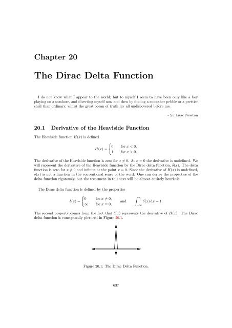
Chapter 20
The Dirac Delta Function
I do not know what I appear to the world; but to myself I seem to have been only like a boy
playing on a seashore, and diverting myself now and then by finding a smoother pebble or a prettier
shell than ordinary, whilst the great ocean of truth lay all undiscovered before me.
20.1 Derivative of the Heaviside Function
The Heaviside function H(x) is defined
H(x) =
�
0 for x < 0�
1 for x > 0.
- Sir Issac Newton
The derivative of the Heaviside function is zero for x �= 0. At x = 0 the derivative is undefined. We
will represent the derivative of the Heaviside function by the Dirac delta function, δ(x). The delta
function is zero for x �= 0 and infinite at the point x = 0. Since the derivative of H(x) is undefined,
δ(x) is not a function in the conventional sense of the word. One can derive the properties of the
delta function rigorously, but the treatment in this text will be almost entirely heuristic.
The Dirac delta function is defined by the properties
�
0 for x �= 0�
δ(x) =
and
∞ for x = 0�
� ∞
δ(x) dx = 1.
The second property comes from the fact that δ(x) represents the derivative of H(x). The Dirac
delta function is conceptually pictured in Figure 20.1.
−∞
Figure 20.1: The Dirac Delta Function.
637

Let f(x) be a continuous function that vanishes at infinity. Consider the integral
� ∞
f(x)δ(x) dx.
−∞
We use integration by parts to evaluate the integral.
� ∞
−∞
f(x)δ(x) dx = � f(x)H(x) � ∞
−∞ −
� ∞
= − f � (x) dx
0
= [−f(x)] ∞ 0
= f(0)
� ∞
f � (x)H(x) dx
We assumed that f(x) vanishes at infinity in order to use integration by parts to evaluate the
integral. However, since the delta function is zero for x �= 0, the integrand is nonzero only at x = 0.
Thus the behavior of the function at infinity should not affect the value of the integral. Thus it is
reasonable that f(0) = � ∞
f(x)δ(x) dx holds for all continuous functions. By changing variables
−∞
and noting that δ(x) is symmetric we can derive a more general formula.
� ∞
f(0) = f(ξ)δ(ξ) dξ
−∞
� ∞
f(x) = f(ξ + x)δ(ξ) dξ
−∞
� ∞
f(x) = f(ξ)δ(ξ − x) dξ
−∞
� ∞
f(x) = f(ξ)δ(x − ξ) dξ
This formula is very important in solving inhomogeneous differential equations.
−∞
20.2 The Delta Function as a Limit
Consider a function b(x� �) defined by
b(x� �) =
The graph of b(x� 1/10) is shown in Figure 20.2.
−∞
�
0 for |x| > �/2
1
�
10
5
for |x| < �/2.
-1 1
Figure 20.2: Graph of b(x� 1/10).
The Dirac delta function δ(x) can be thought of as b(x� �) in the limit as � → 0. Note that the
delta function so defined satisfies the properties,
�
� ∞
0 for x �= 0
δ(x) =
and δ(x) dx = 1
∞ for x = 0
638
−∞

Delayed Limiting Process. When the Dirac delta function appears inside an integral, we can
think of the delta function as a delayed limiting process.
� ∞
� ∞
f(x)δ(x) dx ≡ lim
�→0
f(x)b(x� �) dx.
−∞
Let f(x) be a continuous function and let F � (x) = f(x). We compute the integral of f(x)δ(x).
� ∞
−∞
20.3 Higher Dimensions
−∞
� �/2
1
f(x)δ(x) dx = lim f(x) dx
�→0 � −�/2
1
= lim [F (x)]�/2
�→0 � −�/2
F (�/2) − F (−�/2)
= lim
�→0 �
= F � (0)
= f(0)
We can define a Dirac delta function in n-dimensional Cartesian space, δn(x), x ∈ R n . It is
defined by the following two properties.
δn(x) = 0
�
for x �= 0
δn(x) dx = 1
� n
It is easy to verify, that the n-dimensional Dirac delta function can be written as a product of
1-dimensional Dirac delta functions.
n�
δn(x) = δ(xk)
20.4 Non-Rectangular Coordinate Systems
k=1
We can derive Dirac delta functions in non-rectangular coordinate systems by making a change
of variables in the relation, �
� n
δn(x) dx = 1
Where the transformation is non-singular, one merely divides the Dirac delta function by the Jacobian
of the transformation to the coordinate system.
Example 20.4.1 Consider the Dirac delta function in cylindrical coordinates, (r� θ� z). The Jacobian
is J = r. � ∞ � 2π � ∞
δ3 (x − x0) r dr dθ dz = 1
−∞
For r0 �= 0, the Dirac Delta function is
since it satisfies the two defining properties.
0
0
δ3 (x − x0) = 1
r δ (r − r0) δ (θ − θ0) δ (z − z0)
1
r δ (r − r0) δ (θ − θ0) δ (z − z0) = 0 for (r� θ� z) �= (r0� θ0� z0)
639

� ∞ � 2π � ∞
1
−∞ 0 0 r δ (r − r0) δ (θ − θ0) δ (z − z0) r dr dθ dz
� ∞
� 2π
= δ (r − r0) dr
For r0 = 0, we have
δ3 (x − x0) = 1
δ (r) δ (z − z0)
2πr
since this again satisfies the two defining properties.
0
0
� ∞
δ (θ − θ0) dθ δ (z − z0) dz = 1
−∞
1
2πr δ (r) δ (z − z0) = 0 for (r� z) �= (0� z0)
� ∞ � 2π � ∞
1
2πr δ (r) δ (z − z0) r dr dθ dz = 1
� ∞ � 2π � ∞
δ (r) dr dθ δ (z − z0) dz = 1
2π
−∞
0
0
640
0
0
−∞