Gernot Hoffmann CIE Color Space
Gernot Hoffmann CIE Color Space
Gernot Hoffmann CIE Color Space

Create successful ePaper yourself
Turn your PDF publications into a flip-book with our unique Google optimized e-Paper software.
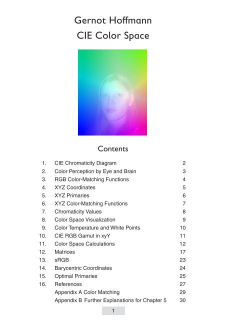
<strong>Gernot</strong> <strong>Hoffmann</strong><br />
<strong>CIE</strong> <strong>Color</strong> <strong>Space</strong><br />
Contents<br />
1. <strong>CIE</strong> Chromaticity Diagram 2<br />
2. <strong>Color</strong> Perception by Eye and Brain 3<br />
3. RGB <strong>Color</strong>-Matching Functions 4<br />
4. XYZ Coordinates 5<br />
5. XYZ Primaries 6<br />
6. XYZ <strong>Color</strong>-Matching Functions 7<br />
7. Chromaticity Values 8<br />
8. <strong>Color</strong> <strong>Space</strong> Visualization 9<br />
9. <strong>Color</strong> Temperature and White Points 10<br />
10. <strong>CIE</strong> RGB Gamut in xyY 11<br />
11. <strong>Color</strong> <strong>Space</strong> Calculations 12<br />
12. Matrices 17<br />
13. sRGB 23<br />
14. Barycentric Coordinates 24<br />
15. Optimal Primaries 25<br />
16. References 27<br />
Appendix A <strong>Color</strong> Matching 29<br />
Appendix B Further Explanations for Chapter 5 30<br />
1
1. <strong>CIE</strong> Chromaticity Diagram (1931)<br />
The threedimensional color space <strong>CIE</strong> XYZ is the basis for all color management systems. This<br />
color space contains all perceivable colors - the human gamut. Many of them cannot be shown<br />
on monitors or printed.<br />
The twodimensional <strong>CIE</strong> chromaticity diagram xyY (below) shows a special projection of the<br />
threedimensional <strong>CIE</strong> color space XYZ.<br />
Some interpretations are possible in xyY, others require the threedimensional space XYZ or the<br />
related threedimensional space <strong>CIE</strong>Lab.<br />
1.0<br />
y<br />
0.9<br />
0.8<br />
0.7<br />
0.6<br />
0.5<br />
0.4<br />
0.3<br />
0.2<br />
0.1<br />
520 525<br />
515 530<br />
535<br />
510<br />
540<br />
545<br />
550<br />
505<br />
555<br />
560<br />
565<br />
500<br />
NTSC <strong>CIE</strong> sRGB<br />
570<br />
575<br />
580<br />
585<br />
495<br />
590<br />
595<br />
600<br />
605<br />
610<br />
490<br />
620<br />
635<br />
700<br />
485<br />
480<br />
475<br />
470<br />
460<br />
380<br />
0.0<br />
0.0 0.1 0.2 0.3 0.4 0.5 0.6 0.7 0.8 0.9 x 1.0<br />
2<br />
sRGB uses ITU-R BT.709 primaries<br />
Red Green Blue White<br />
x 0.64 0.30 0.15 0.3127<br />
y 0.33 0.60 0.06 0.3290<br />
AdobeRGB(98) uses Red and Blue<br />
like sRGB and Green like NTSC<br />
<strong>CIE</strong>-RGB are the primaries for color<br />
matching tests: 700/546.1/435.8nm<br />
Purple line<br />
Wavelengths in nm
2. <strong>Color</strong> Perception by Eye and Brain<br />
The retina contains two groups of sensors, the rods and the cones. In each eye are about 100<br />
millions of rods responsible for the luminance. About 6 millions of cones measure color. The<br />
sensors are already ’wired’ in the retina - only 1 million nerve fibres carry the information to the<br />
brain.The perception of colors by cones requires an absolute luminance of at least some cd/m 2<br />
(candela per squaremeter). A monitor delivers about 100 cd/m 2 for white and 1 cd/m 2 for black.<br />
Three types of cones (together with the rods) form a tristimulus measuring system. Spectral<br />
information is lost and only three color informations are left. We may call these colors blue,<br />
green and red but the red sensor is in fact an orange sensor.<br />
The optical system is not color corrected. It would be impossible to focus simultaneously for<br />
three different wavelengths. The overlapping sensitivities of the green and the red sensor may<br />
indicate that the focussing happens mainly in the overlapping range whereas blue is generally<br />
out of focus. This sounds strange, but the gap for image parts on the blind spot is corrected as<br />
well - another example for the surprising features of eye and brain.<br />
These diagrams show two of several models for the cone sensitivities. These and similar functions<br />
cannot be measured directly - they are mathematical interpretations of color matching<br />
experiments.<br />
The sensitivity between 700nm and 800nm is very low, therefore all the diagrams are drawn for<br />
the range 380nm to 700nm.<br />
10.0<br />
9.0<br />
8.0<br />
7.0<br />
6.0<br />
5.0<br />
4.0<br />
3.0<br />
2.0<br />
1.0<br />
_<br />
p3<br />
0.0<br />
380 420 460 500 540 580 620 λ 660 nm 700<br />
_<br />
p2<br />
_<br />
p1<br />
Cone sensitivities [3]<br />
3<br />
2.0<br />
1.8<br />
1.6<br />
1.4<br />
1.2<br />
1.0<br />
0.8<br />
0.6<br />
0.4<br />
0.2<br />
_<br />
p3<br />
0.0<br />
380 420 460 500 540 580 620 λ 660 nm 700<br />
_<br />
p2<br />
_<br />
p1<br />
Cone sensitivities [1]
3. RGB <strong>Color</strong>-Matching<br />
The color matching experiment was invented by Hermann<br />
Graßmann (1809 - 1877) about 1853.<br />
Three lamps with spectral distributions R,G,B and<br />
weight factors R,G,B =0..100 generate the color<br />
impression C = RR + GG + BB.<br />
The three lamps must have linearly independent<br />
spectra, without any other special specification.<br />
A fourth lamp generates the color impression D.<br />
Can we match the color impressions C and D by<br />
adjusting R,G,B ? In many cases we can:<br />
BlueGreen = 7R + 33G + 39B<br />
In other cases we have to move one of the three lamps<br />
to the left side and match indirectly:<br />
Vibrant BlueGreen +38R = 42G + 91B<br />
Vibrant BlueGreen = -38R + 42G + 91B<br />
This is the introduction of ’negative’ colors. The equal<br />
sign means ’matched by’. It is generally possible to<br />
match a color by three weight factors, but one or even<br />
two can be negative (only one for <strong>CIE</strong>-RGB) .<br />
Data for the example are shown in Appendix A.<br />
The <strong>CIE</strong> Standard Primaries (1931) are narrow band<br />
light sources (monochromats, line spectra or delta<br />
functions) R (700 nm),G (546.1nm) and B (435.8 nm).<br />
They replace the red, green and blue lamps in the<br />
drawing above. In fact these sources were actually<br />
not used - all results were calculated for these primaries<br />
after tests with other sources.<br />
The normalized weight factors are called <strong>CIE</strong> <strong>Color</strong>-<br />
Matching Functions r( λ ) ,g( λ ) ,b( λ ) .<br />
The diagram shows for example the three values for<br />
matching a spectral pure color (monochromat) with<br />
wavelength λ=540nm. This requires a negative value<br />
for red.<br />
RGB colors for a spectrum P(λ) are calculated by<br />
these integrals in the range from 380nm to 700nm or<br />
800nm:<br />
∫<br />
∫<br />
∫<br />
R = k P( λ) r( λ) dλ<br />
G = k P( λ) g( λ) dλ<br />
B = k P( λ) b( λ) dλ<br />
4<br />
View<br />
<strong>Color</strong> D <strong>Color</strong> C<br />
<strong>Color</strong> matching experiment<br />
R,G,B +4.5907<br />
0.4<br />
0.3<br />
0.2<br />
0.1<br />
0.0<br />
+0.0601<br />
+1.0000<br />
300 435.8 546.1 700.0 800<br />
<strong>CIE</strong> Standard Primaries<br />
_<br />
b<br />
-0.1<br />
380 420 460 500 540 580 620 λ 660 nm 700<br />
RGB <strong>Color</strong>-matching functions<br />
_<br />
g<br />
_<br />
r
4. XYZ Coordinates<br />
In order to avoid negative RGB<br />
numbers the <strong>CIE</strong> consortium<br />
had introduced a new coordinate<br />
system XYZ.<br />
The RGB system is essentially<br />
defined by three non-orthogonal<br />
base vectors in XYZ.<br />
The bottom image explains the<br />
sitution for 2D coordinates R,G<br />
and X,Y a little simplified.<br />
The shaded area shows the human<br />
gamut. A plane divides the<br />
space in two half spaces.<br />
The new coordinates X,Y are<br />
chosen so that the gamut is<br />
entirely accessible for positive<br />
values.<br />
This can be generalized for the<br />
3D space.<br />
In the upper image the axes<br />
XYZ are drawn orthogonally, in<br />
the lower image the axes RGB. X<br />
Plane<br />
Y<br />
Z<br />
⎡0.<br />
20000⎤<br />
B ⎢0.<br />
01063⎥<br />
⎣<br />
⎢0.<br />
99000⎦<br />
⎥<br />
RGB base vectors and color cube in XYZ<br />
G<br />
2D visualization for RG and XY<br />
5<br />
⎡0.<br />
49000⎤<br />
R ⎢0.<br />
17697⎥<br />
⎣<br />
⎢0.<br />
00000⎦<br />
⎥<br />
⎡0.<br />
31000⎤<br />
G⎢0.<br />
81240⎥<br />
⎣<br />
⎢0.<br />
01000⎦<br />
⎥<br />
The coordinates of the base vectors in XYZ (coordinates of the primaries as shown above)<br />
for any RGB system are found as columns of the matrix C xr in chapter 11.<br />
R<br />
X
5. XYZ Primaries (see App. B for further Explanations)<br />
The coordinate systems XYZ and RGB are related<br />
to each other by linear equations.<br />
X = Cxr R<br />
X =+ 0. 49000R+ 0. 31000G+ 0. 20000B<br />
Y =+ 0. 17697R+ 0. 81240G+ 0.01063B<br />
() 1<br />
Z =+ 0. 00000R+ 0. 01000G+ 0. 99000B<br />
R = Crx X<br />
R =+ 2. 36461X−0. 89654 Y−0. 46807 Z<br />
G =− 0. 51517 X+ 1. 42641Y+ 0. 08876 Z ( 2)<br />
B =+ 0. 00520<br />
X− 0. 01441Y+ 1. 00920 Z<br />
Another view is possible by introducing synthetical<br />
or ’imaginary’ primaries X,Y,Z.<br />
The Standard Primaries R, G, B are monochromatic<br />
stimuli. Mathematically they are single delta functions<br />
with well defined areas.<br />
In the diagram the height represents the contribution<br />
to the luminance.<br />
The ratios are 1.0:4.5907:0.0601.<br />
The spectra X,Y,Z are calculated by the application<br />
of the matrix operation (2) and the scale factors.<br />
An example:<br />
X=1, Y=0, Z=0 :<br />
X =+ 2. 36461⋅ 1. 0000R<br />
−0. 51517⋅4. 5907G<br />
+ 0. 00520⋅0. 0601B<br />
X =+ 2. 36461R<br />
− 2. 36499G + 0. 00031B<br />
The primaries X,Y,Z are sums of delta functions.<br />
X and Z do not contribute to the luminance. This is<br />
a special trick in the <strong>CIE</strong> system. The integrals are<br />
zero, here represented by the sum of the heights.<br />
The luminance is defined by Y only.<br />
In color matching experiments negative values or<br />
weight factors R, G, B are allowed.<br />
Some matchable colors cannot be generated by the<br />
Standard Primaries. Other light sources are necessary,<br />
especially spectral pure sources (monochromats).<br />
6<br />
R,G,B +4.5907<br />
X<br />
Y<br />
Z<br />
+0.0601<br />
+0.00031<br />
-0.00087<br />
0.06065<br />
-2.36499<br />
+6.54822<br />
0.40747<br />
+1.0000<br />
300 435.8 546.1 700.0 800<br />
<strong>CIE</strong> primaries R,G,B<br />
+2.36461<br />
-0.89654<br />
-0.46807<br />
Synthetical primaries X,Y, Z
6. XYZ <strong>Color</strong>-Matching Functions<br />
The new color-matching functions x( λ ) , y( λ ) ,z( λ ) have non-negative values, as expected.<br />
They are calculated from r( λ ) ,g( λ ) ,b( λ ) by using the matrix Cxr in chapter 5.<br />
The functions x( λ ) , y( λ ) ,z( λ ) can be understood as<br />
weight factors. For a spectral pure color C with a<br />
fixed wavelength λ read in the diagram the three<br />
values. Then the color can be mixed by the three<br />
Standard Primaries:<br />
C = x( λ ) X + y( λ ) Y + z( λ ) Z<br />
Generally we write<br />
C = X X + Y Y + Z Z<br />
and a given spectral color distribution P(λ) delivers<br />
the three coordinates XYZ by these integrals in the<br />
range from 380nm to 700nm or 800nm:<br />
∫<br />
∫<br />
∫<br />
X = k P( λ) x( λ) dλ<br />
Y = k P( λ) y( λ) dλ<br />
Z = k P( λ) z( λ) dλ<br />
7<br />
2.0<br />
1.8<br />
1.6<br />
1.4<br />
1.2<br />
1.0<br />
0.8<br />
0.6<br />
0.4<br />
0.2<br />
_<br />
z<br />
0.0<br />
380 420 460 500 540 580 620 λ 660 nm 700<br />
XYZ <strong>Color</strong>-matching functions<br />
Mostly, the arbitrary factor k is chosen for a normalized value Y=1 or Y=100. Matrix operations<br />
are always normalized for R,G,B,Y=0 to 1.<br />
This diagram shows already the human gamut in XYZ. It is an irregularly shaped cone.The<br />
intersection with the blue-ish colored plane in the corner will deliver the chromaticity diagram.<br />
X Y<br />
Human gamut in XYZ<br />
_<br />
y<br />
_<br />
x
7. Chromaticity Values<br />
The chromaticity values x,y,z depend only on the<br />
hue or dominant wavelength and the saturation.<br />
They are independend of the luminance:<br />
x<br />
y<br />
z<br />
X<br />
=<br />
X+ Y+ Z<br />
Y<br />
=<br />
X+ Y+ Z<br />
Z<br />
=<br />
X+ Y+ Z<br />
Obviously we have x + y + z = 1. All the values are<br />
on the triangle plane, projected by a line through<br />
the arbitrary color XYZ and the origin, if we draw<br />
XYZ and xyz in one diagram.<br />
This is a planar projection. The center of projection<br />
is in the origin.<br />
8<br />
1<br />
z<br />
View<br />
Arbitrary<br />
color XYZ<br />
Projection and chromaticity plane<br />
The vertical projection onto the xy-plane is the chromaticity diagram xyY (view direction).<br />
To reconstruct a color triple XYZ from the chromaticity values xy we need an additional<br />
information, the luminance Y.<br />
z x y<br />
X x<br />
y Y<br />
= 1−<br />
−<br />
=<br />
Z<br />
=<br />
z<br />
y Y<br />
All visible (matchable) colors which differ only by Z<br />
luminance map to the same point in the chromaticity<br />
diagram. This is sometimes called ’horseshoe<br />
diagram’ (page 2).<br />
The right image shows a 3D view of the colormatching<br />
functions, connected by rays with the<br />
origin. The contour is here called ‘locus of unit monochromats’<br />
[18]. For spectral colors this is the same<br />
as XYZ.<br />
Then the contour is mapped onto the plane as<br />
above.<br />
The spectral loci for blue and for red end nearly in<br />
the origin: colors with short and long wavelengths<br />
appear rather dark, they are almost invisible for a<br />
reasonably limited power.<br />
The chromaticity diagram conceals this important<br />
fact. The purple line can be considered as a fake.<br />
Real purples are inside the horseshoe contour. X<br />
1<br />
1<br />
y<br />
Y<br />
x<br />
Rendering primaries<br />
445<br />
535<br />
606<br />
Halfaxis length 1.0
8. <strong>Color</strong> <strong>Space</strong> Visualization<br />
These images are computer graphics. Accurate transformations and a few applications of<br />
image processing.The contour of the horseshoe is mapped to XYZ for luminances Y = 0..1 .<br />
The purple plane is shown transparent. All colors were selected for readabilty. The colors are<br />
not correct, this is anyway impossible. More important is here the geometry. The gamut volume<br />
is confined by the color surface (pure spectral colors), the purple plane and the plane Y = 1.<br />
The regions with small values Y appear extremely distorted - near to a singularity.<br />
For blue very high values Z are necessary to match a color with specified luminance Y = 1.<br />
X<br />
2<br />
1 1<br />
Z<br />
X Y<br />
9<br />
2<br />
Y
9. <strong>Color</strong> Temperature and White Points<br />
The graphic shows the color temperature for the Planck radiator from 2000K to 10000K, the<br />
directions of correlated color temperatures and the white points for daylight D50 and D65.<br />
Uncalibrated monitors have about 9300K which is here simply called D93.<br />
Data by [3]. EPS graphic available here [15].<br />
1.0<br />
y<br />
0.9<br />
0.8<br />
0.7<br />
0.6<br />
0.5<br />
0.4<br />
0.3<br />
0.2<br />
0.1<br />
T/K x y Dir y/x<br />
2000 0.52669 0.41331 1.33101<br />
2105 0.51541 0.41465 1.39021<br />
2222 0.50338 0.41525 1.45962<br />
2353 0.49059 0.41498 1.54240<br />
2500 0.47701 0.41368 1.64291<br />
2677 0.463 0.41121 1.76811 % error in table [3], estimated values<br />
2857 0.446 0.40742 1.92863<br />
3077 0.43156 0.40216 2.14300<br />
3333 0.41502 0.39535 2.44455<br />
3636 0.39792 0.38690 2.90309<br />
4000 0.38045 0.37676 3.68730<br />
4444 0.36276 0.36496 5.34398<br />
5000 0.34510 0.35162 11.17883<br />
5714 0.32775 0.33690 -39.34888<br />
6667 0.31101 0.32116 -6.18336<br />
8000 0.29518 0.30477 -3.08425<br />
10000 0.28063 0.28828 -1.93507<br />
520 525<br />
515 530<br />
535<br />
510<br />
540<br />
545<br />
550<br />
505<br />
555<br />
560<br />
565<br />
500<br />
570<br />
575<br />
580<br />
585<br />
495<br />
490<br />
D50<br />
D65<br />
D93<br />
590<br />
595<br />
600<br />
605<br />
610<br />
620<br />
635<br />
700<br />
485<br />
480<br />
475<br />
470<br />
460<br />
380<br />
10000<br />
8000<br />
6667<br />
5714<br />
5000<br />
4444<br />
4000<br />
3636<br />
3333<br />
3077<br />
2857<br />
2677<br />
2500<br />
2353<br />
2222<br />
2105<br />
2000<br />
0.0<br />
0.0 0.1 0.2 0.3 0.4 0.5 0.6 0.7 0.8 0.9 x 1.0<br />
10
10. <strong>CIE</strong> RGB Gamut in xyY<br />
The gamut of any RGB system is mostly visualized by a triangle in xyY. For different luminances<br />
Y=const. we get the intersection of a vertical plane and the RGB cube (chapter 4). The<br />
intersection delivers a triangle, a quadriliteral, a pentagon or a hexagon. These polygons are<br />
projected onto the xy-plane<br />
The chromaticity diagram below shows the actual gamut for different luminances Y. Low<br />
luminances seem to produce a large gamut. But that is a fake - a result of the perspective<br />
projection from XYZ to xyY.<br />
The gamut appears similarly in all RGB systems. A color outside the triangle (which is defined<br />
by the primaries) is always out-of-gamut. A color inside the triangle is not necessarily ingamut.<br />
1.0<br />
y<br />
0.9<br />
0.8<br />
0.7<br />
0.6<br />
0.5<br />
0.4<br />
0.3<br />
0.2<br />
0.1<br />
520 525<br />
515 530<br />
535<br />
510<br />
540<br />
545<br />
550<br />
505<br />
555<br />
560<br />
565<br />
500<br />
570<br />
575<br />
580<br />
585<br />
495<br />
Y = 0.05 .. 0.95<br />
0.85<br />
0.75<br />
0.95<br />
590<br />
595<br />
600<br />
605<br />
610<br />
490<br />
0.65<br />
0.55<br />
620<br />
635<br />
700<br />
485<br />
0.45<br />
0.35<br />
0.25<br />
480<br />
0.15<br />
475<br />
470<br />
0.05<br />
460<br />
380<br />
0.0<br />
0.0 0.1 0.2 0.3 0.4 0.5 0.6 0.7 0.8 0.9 x 1.0<br />
11
11.1 <strong>Color</strong> <strong>Space</strong> Calculations / General<br />
In this chapter we derive the relations between <strong>CIE</strong> xyY, <strong>CIE</strong> XYZ and any arbitrary RGB<br />
space. It is essential to understand the principle of RGB basis vectors in the XYZ coordinate<br />
system. This was shown on previous pages.<br />
Given are the coordinates for the primaries in <strong>CIE</strong> xyY and for the white point:<br />
x r ,y r ,x g ,y g ,x b ,y b ,x w ,y w . <strong>CIE</strong> xyY is the horseshoe diagram. Furtheron we need the<br />
luminance V.<br />
We want to derive the relation between any color set r,g,b and the coordinates X,Y,Z .<br />
() 1 r = (, rgb , )<br />
( 2)<br />
X = ( XYZ , , )<br />
( 3)<br />
x = ( xyz , , )<br />
( 4)<br />
( 8) X = Vx/ y<br />
Y = V<br />
Z = Vz/ y<br />
T<br />
T<br />
T<br />
L = X+ Y+ Z<br />
( 5)<br />
x = X/ L<br />
y = Y/ L<br />
z = Z/ L<br />
( 6) z = 1−x−y<br />
( 7)<br />
X = L x<br />
( 9) R = Lx = L( x , y , z )<br />
r r r r T<br />
<strong>Color</strong> values in RGB<br />
<strong>Color</strong> values in XYZ<br />
<strong>Color</strong> values in xyY<br />
Scaling value<br />
V is the luminance of the stimulus, according to the luminous efficiency function V(λ) in [3].<br />
We should not call this immediately Y because Y is mostly normalized for 1 or 100.<br />
Basis vectors for the primaries and white point in XYZ:<br />
G = Lx = L( x , y , z )<br />
g g g g T<br />
B = Lx = L( x , y , z )<br />
b b b b T<br />
( 10) W = Lw = L( x , y , z )<br />
( 11) u = ( uvw , , )<br />
T<br />
w w w T<br />
Set of scale factors for the white point correction:<br />
12
11.2 <strong>Color</strong> <strong>Space</strong> Calculations / General<br />
For the white point correction, the basis vectors R,G,B are scaled by u,v,w. This does not<br />
change their coordinates in xyY .The mapping from XYZ to xyY is a central planar projection.<br />
T<br />
( 12) X = L( x, y, z) = ruR+ gvG+ bwB<br />
For the white point we have r = g = b = 1.<br />
( 13) W = Lx ( , y , z ) = Lux ( , y, z) + Lvx ( , y, z) + Lwx ( , y, z<br />
( 14)<br />
⎡x<br />
⎢y<br />
⎣<br />
⎢z<br />
w<br />
w<br />
w<br />
⎤<br />
⎥<br />
⎦<br />
⎥ =<br />
( 15) w = 1−u−v<br />
w w w T<br />
⎡x<br />
x x<br />
⎢y<br />
y y<br />
⎢<br />
⎣z<br />
z z<br />
r g b<br />
r g b<br />
r g b<br />
⎤ ⎡ u ⎤<br />
⎥ ⎢ v ⎥<br />
⎥<br />
w<br />
⎦ ⎣<br />
⎢<br />
⎦<br />
⎥<br />
r r r T<br />
This can be re-arranged, L cancels on both sides.:<br />
⎡ u ⎤<br />
= P ⎢ v ⎥<br />
⎣<br />
⎢w⎦<br />
⎥<br />
⎡x<br />
w ⎤<br />
( 16)<br />
⎢y<br />
w ⎥<br />
⎣<br />
⎢<br />
⎦<br />
⎥<br />
xr yr xg yg xb<br />
u<br />
yb<br />
v<br />
1 u v<br />
=<br />
⎡<br />
⎢<br />
⎢<br />
⎣<br />
⎤ ⎡ ⎤<br />
⎥ ⎢ ⎥<br />
⎥<br />
⎦ ⎣<br />
⎢ − − ⎦<br />
⎥<br />
( 17) x = ( x − x ) u + ( x − x ) v + x<br />
w r b g b b<br />
y = ( y − y ) u+ ( y − y ) v+ y<br />
w r b g b b<br />
These linear equations are solved by Cramer’s rule.<br />
( 18) D = ( xr −xb) ( yg −yb) −( yr −yb) ( xg −xb)<br />
U = ( x −x )( y −y ) −( y − y )( x − x )<br />
w b g b w b<br />
g b<br />
V = ( xr −xb) ( yw −yb) −( yr −yb) ( xw −xb)<br />
( 19)<br />
u = U/ D<br />
v = V/ D<br />
w = 1−u−v 13<br />
g g g T<br />
b b b) T<br />
It is not necessary to invert the whole matrix numerically. We can simplify the calculation by<br />
adding the first two rows to the third row and find so immediately Eq.(15), which is anyway<br />
clear:<br />
In the next step we assume that u,v,w are already calculated and we use the general color<br />
transformation Eq.(12) and furtheron Eq.(8). We get the matrices C xr and C rx .<br />
⎡X⎤<br />
( 20)<br />
⎢Y⎥<br />
⎣<br />
⎢Z⎦<br />
⎥<br />
ux / y<br />
V uy / y<br />
uzr / y<br />
vx<br />
vy<br />
/ y<br />
/ y<br />
wx<br />
wy<br />
/ y<br />
/ y<br />
=<br />
⎡<br />
⎢<br />
⎢<br />
⎣ vz / y wz / y<br />
( 21 X = VC<br />
r<br />
xr<br />
−<br />
xr<br />
r w g w b w<br />
r w g w b w<br />
w g w b w<br />
( 22) r = ( 1/<br />
V)<br />
C 1<br />
X = (/ 1 ) C X<br />
V rx<br />
⎤ ⎡r<br />
⎤<br />
⎥ ⎢g⎥<br />
⎥<br />
b<br />
⎦ ⎣<br />
⎢<br />
⎦<br />
⎥
11.3 <strong>Color</strong> <strong>Space</strong> Calculations / General<br />
For better readability we show the last two equations again, but now with V=1, as in most<br />
publications.<br />
( 23)<br />
X = C r<br />
xr<br />
−1<br />
xr rx<br />
( 24)<br />
r = C X = C X<br />
Now we can easily derive the relation between two different RGB spaces, e.g. working spaces<br />
and image source spaces.<br />
( 25)<br />
X = C r<br />
( 26)<br />
X = C r<br />
xr1<br />
1<br />
2<br />
2 2<br />
2<br />
1<br />
=<br />
xr<br />
−<br />
xr xr1<br />
1<br />
( 27)<br />
r C C r<br />
( 28)<br />
r = C r<br />
2 21 1<br />
An example shows the conversion of Rec.709/D65 to D50 and D93. The resulting matrix<br />
C 21 is diagonal, because the source and destination primaries are the same. The explanation<br />
as above is valid for the representation of the same physical color in two different RGB systems.<br />
For the simulation of D50 or D93 effects in the same D65 RGB system one has to apply the<br />
inverse matrix.<br />
Rec.709<br />
xr= 0.6400 yr= 0.3300 zr= 0.0300<br />
xg= 0.3000 yg= 0.6000 zg= 0.1000<br />
xb= 0.1500 yb= 0.0600 zb= 0.7900<br />
D65<br />
xw= 0.3127 yw= 0.3290 zw= 0.3583<br />
D50<br />
xw= 0.3457 yw= 0.3585 zw= 0.2958<br />
Matrix Cxr: X=Cxr*R65<br />
0.4124 0.3576 0.1805<br />
0.2126 0.7152 0.0722<br />
0.0193 0.1192 0.9505<br />
Matrix Crx: R65=Crx*X<br />
3.2410 -1.5374 -0.4986<br />
-0.9692 1.8760 0.0416<br />
0.0556 -0.2040 1.0570<br />
Matrix Dxr: X=Dxr*R50<br />
0.4852 0.3489 0.1303<br />
0.2502 0.6977 0.0521<br />
0.0227 0.1163 0.6861<br />
Matrix Drx: R50=Drx*X<br />
2.7548 -1.3068 -0.4238<br />
-0.9935 1.9229 0.0426<br />
0.0771 -0.2826 1.4644<br />
Matrix Err: R50=Err*R65=Drx*Cxr*R65<br />
0.8500 0.0000 0.0000<br />
0.0000 1.0250 0.0000<br />
0.0000 0.0000 1.3855<br />
Matrix Frr: R65=Frr*R50=Crx*Dxr*R50<br />
1.1765 0.0000 0.0000<br />
0.0000 0.9756 0.0000<br />
0.0000 0.0000 0.7218<br />
14<br />
Rec.709<br />
xr= 0.6400 yr= 0.3300 zr= 0.0300<br />
xg= 0.3000 yg= 0.6000 zg= 0.1000<br />
xb= 0.1500 yb= 0.0600 zb= 0.7900<br />
D65<br />
xw= 0.3127 yw= 0.3290 zw= 0.3583<br />
D93<br />
xw= 0.2857 yw= 0.2941 zw= 0.4202<br />
Matrix Cxr: X=Cxr*R65<br />
0.4124 0.3576 0.1805<br />
0.2126 0.7152 0.0722<br />
0.0193 0.1192 0.9505<br />
Matrix Crx: R65=Crx*X<br />
3.2410 -1.5374 -0.4986<br />
-0.9692 1.8760 0.0416<br />
0.0556 -0.2040 1.0570<br />
Matrix Dxr: X=Dxr*R93<br />
0.3706 0.3554 0.2455<br />
0.1911 0.7107 0.0982<br />
0.0174 0.1185 1.2929<br />
Matrix Drx: R93=Drx*X<br />
3.6066 -1.7108 -0.5549<br />
-0.9753 1.8877 0.0418<br />
0.0409 -0.1500 0.7771<br />
Matrix Err: R93=Err*R65=Drx*Cxr*R65<br />
1.1128 0.0000 0.0000<br />
0.0000 1.0063 0.0000<br />
0.0000 0.0000 0.7352<br />
Matrix Frr: R65=Frr*R93=Crx*Dxr*R93<br />
0.8986 0.0000 0.0000<br />
0.0000 0.9938 0.0000<br />
0.0000 0.0000 1.3602
11.4 <strong>Color</strong> <strong>Space</strong> Calculations / Simplified<br />
Now we clean up the mathematics. Eq.(14) delivers:<br />
( 29)<br />
−1<br />
u = P w<br />
Eq.(12) and Eq.(20) can be written using the diagonal matrix D with elements u/y w etc.:<br />
( 30)<br />
X = PDr<br />
( 31)<br />
X C r<br />
= xr<br />
Together with Eq.(29) we find this simple formula for the matrix C xr :<br />
⎡u/<br />
yw<br />
0 0<br />
( 32)<br />
Cxr = P⎢0<br />
v/ yw<br />
0<br />
⎣<br />
⎢ 0 0 w/ y<br />
w<br />
⎤<br />
⎥<br />
⎦<br />
⎥<br />
The examples in chapter 12 were written by Pascal. Here is a new example in MatLab.<br />
Calculation of the matrices for sRGB:<br />
% G.<strong>Hoffmann</strong><br />
% January 14 / 2005<br />
% Matrix Cxr and Crx for sRGB<br />
xr=0.6400; yr=0.3300; zr=1-xr-yr;<br />
xg=0.3000; yg=0.6000; zg=1-xg-yg;<br />
xb=0.1500; yb=0.0600; zb=1-xb-yb;<br />
xw=0.3127; yw=0.3290; zw=1-xw-yw;<br />
W=[xw; yw; zw];<br />
P=[xr xg xb;<br />
yr yg yb;<br />
zr zg zb];<br />
u=inv(P)*W<br />
% D=[u(1) 0 0;<br />
% 0 u(2) 0;<br />
% 0 0 u(3)]/yw<br />
D=diag(u/yw)<br />
Cxr=P*D<br />
Crx=inv(Cxr)<br />
% Result:<br />
% Cxr 0.4124 0.3576 0.1805<br />
% 0.2126 0.7152 0.0722<br />
% 0.0193 0.1192 0.9505<br />
% Crx 3.2410 -1.5374 -0.4986<br />
% -0.9692 1.8760 0.0416<br />
% 0.0556 -0.2040 1.0570<br />
15
11.5 <strong>Color</strong> <strong>Space</strong> Calculations / Application<br />
The task: red, green and blue lasers generate monochromatic light at wavelengths 671nm,<br />
532nm and 473nm. The powers are to be adjusted so that the three lasers together deliver<br />
white light D65. Calculate the matrices, the radiant power ratios and the photometric ratios.<br />
In order to test the algorithms we are doing the same for <strong>CIE</strong> primaries and Equal Energy<br />
White, just as if the lasers had these primaries. The results are known in advance, based on<br />
standard text books. Thanks to Gerhard Fuernkranz for important clarifications.<br />
<strong>CIE</strong> primaries and white point E<br />
% G.<strong>Hoffmann</strong><br />
% January 19 / 2005<br />
% Calculations for <strong>CIE</strong> primaries<br />
% x-bar,y-bar,z-bar interpolated<br />
% 700.0 546.1 435.8 nm<br />
xbr=0.011359; xbg=0.375540; xbb=0.333181;<br />
ybr=0.004102; ybg=0.984430; ybb=0.017769;<br />
zbr=0.000000; zbg=0.012207; zbb=1.649716;<br />
% Equal Energy WP<br />
Xw=1; Yw=1; Zw=1;<br />
%Chromaticity coordinates<br />
D=xbr+ybr+zbr; xr=xbr/D; yr=ybr/D; zr=zbr/D;<br />
D=xbg+ybg+zbg; xg=xbg/D; yg=ybg/D; zg=zbg/D;<br />
D=xbb+ybb+zbb; xb=xbb/D; yb=ybb/D; zb=zbb/D;<br />
D=Xw +Yw+ Zw; xw=Xw/D; yw=Yw/D; zw=Zw/D;<br />
w=[xw; yw; zw];<br />
P=[xr xg xb;<br />
yr yg yb;<br />
zr zg zb];<br />
u=inv(P)*w<br />
D=diag(u/yw)<br />
Cxr=P*D<br />
% 0.4902 0.3099 0.1999<br />
% 0.1770 0.8123 0.0107<br />
% 0.0000 0.0101 0.9899<br />
Crx=inv(Cxr)<br />
% 2.3635 -0.8958 -0.4677<br />
% -0.5151 1.4265 0.0887<br />
% 0.0052 -0.0145 1.0093<br />
% Radiant power ratios<br />
Xbar=[xbr xbg xbb;<br />
ybr ybg ybb;<br />
zbr zbg zbb];<br />
W=[Xw; Yw; Zw];<br />
R=inv(Xbar)*W<br />
R=R/R(3)<br />
% 71.9166 1.3751 1.0000<br />
% 72.0962 1.3791 1.0000 Wyszecki & Stiles<br />
% Luminous efficiency ratios<br />
L=[R(1)*ybr; R(2)*ybg; R(3)*ybb]<br />
L=L/L(1)<br />
% 1.0000 4.5889 0.0602<br />
% 1.0000 4.5907 0.0601 Wyszecki & Stiles<br />
16<br />
Laser primaries and white point D65<br />
% G.<strong>Hoffmann</strong><br />
% January 19 / 2005<br />
% Calculations for Laser primaries<br />
% x-bar,y-bar,z-bar interpolated<br />
% 671 532 473 nm<br />
xbr=0.0819; xbg=0.1891; xbb=0.1627;<br />
ybr=0.0300; ybg=0.8850; ybb=0.1034;<br />
zbr=0.0000; zbg=0.0369; zbb=1.1388;<br />
% D65<br />
Xw=0.9504; Yw=1.0000; Zw=1.0890;<br />
%Chromaticity coordinates<br />
D=xbr+ybr+zbr; xr=xbr/D; yr=ybr/D; zr=zbr/D;<br />
D=xbg+ybg+zbg; xg=xbg/D; yg=ybg/D; zg=zbg/D;<br />
D=xbb+ybb+zbb; xb=xbb/D; yb=ybb/D; zb=zbb/D;<br />
D=Xw +Yw+ Zw; xw=Xw/D; yw=Yw/D; zw=Zw/D;<br />
w=[xw; yw; zw];<br />
P=[xr xg xb;<br />
yr yg yb;<br />
zr zg zb];<br />
u=inv(P)*w<br />
D=diag(u/yw)<br />
Cxr=P*D<br />
% 0.6571 0.1416 0.1516<br />
% 0.2407 0.6629 0.0964<br />
% 0 0.0276 1.0614<br />
Crx=inv(Cxr)<br />
% 1.6476 -0.3435 -0.2042<br />
% -0.6005 1.6394 -0.0631<br />
% 0.0156 -0.0427 0.9438<br />
% Radiant power ratios<br />
Xbar=[xbr xbg xbb;<br />
ybr ybg ybb;<br />
zbr zbg zbb];<br />
W=[Xw; Yw; Zw];<br />
R=inv(Xbar)*W<br />
R=R/R(1)<br />
% 1.0000 0.0934 0.1162<br />
R=R/R(2)<br />
% 10.7111 1.0000 1.2442<br />
R=R/R(3)<br />
% 8.6088 0.8037 1.0000<br />
% Luminous efficiency ratios<br />
L=[R(1)*ybr; R(2)*ybg; R(3)*ybb];<br />
L=L/L(1)<br />
% 1.0000 2.7542 0.4004<br />
L=L/L(2)<br />
% 0.3631 1.0000 0.1454<br />
L=L/L(3)<br />
% 2.4977 6.8791 1.0000
12.1 Matrices / <strong>CIE</strong> + E<br />
<strong>CIE</strong> Primaries and white point E [3]. Page 5 shows the same results.<br />
Data are in the Pascal source code.<br />
Program CiCalcCi;<br />
{ Calculations RGB—<strong>CIE</strong> }<br />
{ G.<strong>Hoffmann</strong> February 01, 2002 }<br />
Uses Crt,Dos,Zgraph00;<br />
Var r,g,b,x,y,z,u,v,w,d : Extended;<br />
i,j,k,flag : Integer;<br />
xr,yr,zr,xg,yg,zg,xb,yb,zb,xw,yw,zw : Extended;<br />
prn,cie : Text;<br />
Var Cxr,Crx: ANN;<br />
Begin<br />
ClrScr;<br />
{ <strong>CIE</strong> Primaries }<br />
xr:=0.73467;<br />
yr:=0.26533;<br />
zr:=1-xr-yr;<br />
xg:=0.27376;<br />
yg:=0.71741;<br />
zg:=1-xg-yg;<br />
xb:=0.16658;<br />
yb:=0.00886;<br />
zb:=1-xb-yb;<br />
{ <strong>CIE</strong> White Point }<br />
xw:=1/3;<br />
yw:=1/3;<br />
zw:=1-xw-yw;<br />
{ White Point Correction }<br />
D:=(xr-xb)*(yg-yb)-(yr-yb)*(xg-xb);<br />
U:=(xw-xb)*(yg-yb)-(yw-yb)*(xg-xb);<br />
V:=(xr-xb)*(yw-yb)-(yr-yb)*(xw-xb);<br />
u:=U/D;<br />
v:=V/D;<br />
w:=1-u-v;<br />
{ Matrix Cxr }<br />
Cxr[1,1]:=u*xr/yw; Cxr[1,2]:=v*xg/yw; Cxr[1,3]:=w*xb/yw;<br />
Cxr[2,1]:=u*yr/yw; Cxr[2,2]:=v*yg/yw; Cxr[2,3]:=w*yb/yw;<br />
Cxr[3,1]:=u*zr/yw; Cxr[3,2]:=v*zg/yw; Cxr[3,3]:=w*zb/yw;<br />
{ Matrix Crx }<br />
HoInvers (3,Cxr,Crx,D,flag);<br />
Assign (prn,’C:\CiMalcCi.txt’); ReWrite(prn);<br />
Writeln (prn,’ Matrix Cxr’);<br />
Writeln (prn,Cxr[1,1]:12:4, Cxr[1,2]:12:4, Cxr[1,3]:12:4);<br />
Writeln (prn,Cxr[2,1]:12:4, Cxr[2,2]:12:4, Cxr[2,3]:12:4);<br />
Writeln (prn,Cxr[3,1]:12:4, Cxr[3,2]:12:4, Cxr[3,3]:12:4);<br />
Writeln (prn,’ Matrix Crx’);<br />
Writeln (prn,Crx[1,1]:12:4, Crx[1,2]:12:4, Crx[1,3]:12:4);<br />
Writeln (prn,Crx[2,1]:12:4, Crx[2,2]:12:4, Crx[2,3]:12:4);<br />
Writeln (prn,Crx[3,1]:12:4, Crx[3,2]:12:4, Crx[3,3]:12:4);<br />
Close(prn);<br />
Readln;<br />
End.<br />
Matrix Cxr<br />
X 0.4900 0.3100 0.2000<br />
Y 0.1770 0.8124 0.0106<br />
Z -0.0000 0.0100 0.9900<br />
Matrix Crx<br />
R 2.3647 -0.8966 -0.4681<br />
G -0.5152 1.4264 0.0887<br />
B 0.0052 -0.0144 1.0092<br />
X = C xr R<br />
R = C rx X<br />
17
12.2 Matrices / 709 + D65 / sRGB<br />
ITU-R BT.709 Primaries and white point D65 [9]. Valid for sRGB.<br />
Data are in the Pascal source code.<br />
Program CiCalc65;<br />
{ Calculations RGB—<strong>CIE</strong> }<br />
{ G.<strong>Hoffmann</strong> February 01, 2002 }<br />
Uses Crt,Dos,Zgraph00;<br />
Var r,g,b,x,y,z,u,v,w,d : Extended;<br />
i,j,k,flag : Integer;<br />
xr,yr,zr,xg,yg,zg,xb,yb,zb,xw,yw,zw : Extended;<br />
prn,cie : Text;<br />
Var Cxr,Crx: ANN;<br />
Begin<br />
ClrScr;<br />
{ Rec 709 Primaries }<br />
xr:=0.6400;<br />
yr:=0.3300;<br />
zr:=1-xr-yr;<br />
xg:=0.3000;<br />
yg:=0.6000;<br />
zg:=1-xg-yg;<br />
xb:=0.1500;<br />
yb:=0.0600;<br />
zb:=1-xb-yb;<br />
{ D65 White Point }<br />
xw:=0.3127;<br />
yw:=0.3290;<br />
zw:=1-xw-yw;<br />
{ White Point Correction }<br />
D:=(xr-xb)*(yg-yb)-(yr-yb)*(xg-xb);<br />
U:=(xw-xb)*(yg-yb)-(yw-yb)*(xg-xb);<br />
V:=(xr-xb)*(yw-yb)-(yr-yb)*(xw-xb);<br />
u:=U/D;<br />
v:=V/D;<br />
w:=1-u-v;<br />
{ Matrix Cxr }<br />
Cxr[1,1]:=u*xr/yw; Cxr[1,2]:=v*xg/yw; Cxr[1,3]:=w*xb/yw;<br />
Cxr[2,1]:=u*yr/yw; Cxr[2,2]:=v*yg/yw; Cxr[2,3]:=w*yb/yw;<br />
Cxr[3,1]:=u*zr/yw; Cxr[3,2]:=v*zg/yw; Cxr[3,3]:=w*zb/yw;<br />
{ Matrix Crx }<br />
HoInvers (3,Cxr,Crx,D,flag);<br />
Assign (prn,’C:\CiMalc65.txt’); ReWrite(prn);<br />
Writeln (prn,’ Matrix Cxr’);<br />
Writeln (prn,Cxr[1,1]:12:4, Cxr[1,2]:12:4, Cxr[1,3]:12:4);<br />
Writeln (prn,Cxr[2,1]:12:4, Cxr[2,2]:12:4, Cxr[2,3]:12:4);<br />
Writeln (prn,Cxr[3,1]:12:4, Cxr[3,2]:12:4, Cxr[3,3]:12:4);<br />
Writeln (prn,’ Matrix Crx’);<br />
Writeln (prn,Crx[1,1]:12:4, Crx[1,2]:12:4, Crx[1,3]:12:4);<br />
Writeln (prn,Crx[2,1]:12:4, Crx[2,2]:12:4, Crx[2,3]:12:4);<br />
Writeln (prn,Crx[3,1]:12:4, Crx[3,2]:12:4, Crx[3,3]:12:4);<br />
Close(prn);<br />
Readln;<br />
End.<br />
Matrix Cxr<br />
X 0.4124 0.3576 0.1805<br />
Y 0.2126 0.7152 0.0722<br />
Z 0.0193 0.1192 0.9505<br />
Matrix Crx<br />
R 3.2410 -1.5374 -0.4986<br />
G -0.9692 1.8760 0.0416<br />
B 0.0556 -0.2040 1.0570<br />
X = C xr R<br />
R = C rx X<br />
18
12.3 Matrices / AdobeRGB + D65<br />
AdobeRGB(98), D65.<br />
Data are in the Pascal source code.<br />
Program CiCalc98;<br />
{ Calculations RGB—AdobeRGB98 }<br />
{ G.<strong>Hoffmann</strong> März 28, 2004 }<br />
Uses Crt,Dos,Zgraph00;<br />
Var r,g,b,x,y,z,u,v,w,d : Double;<br />
i,j,k,flag : Integer;<br />
xr,yr,zr,xg,yg,zg,xb,yb,zb,xw,yw,zw : Double;<br />
prn,cie : Text;<br />
Var Cxr,Crx: ANN;<br />
Begin<br />
ClrScr;<br />
{ AdobeRGB(98) }<br />
xr:=0.6400;<br />
yr:=0.3300;<br />
zr:=1-xr-yr;<br />
xg:=0.2100;<br />
yg:=0.7100;<br />
zg:=1-xg-yg;<br />
xb:=0.1500;<br />
yb:=0.0600;<br />
zb:=1-xb-yb;<br />
{ D65 White Point }<br />
xw:=0.3127;<br />
yw:=0.3290;<br />
zw:=1-xw-yw;<br />
{ White Point Correction }<br />
D:=(xr-xb)*(yg-yb)-(yr-yb)*(xg-xb);<br />
U:=(xw-xb)*(yg-yb)-(yw-yb)*(xg-xb);<br />
V:=(xr-xb)*(yw-yb)-(yr-yb)*(xw-xb);<br />
u:=U/D;<br />
v:=V/D;<br />
w:=1-u-v;<br />
{ Matrix Cxr }<br />
Cxr[1,1]:=u*xr/yw; Cxr[1,2]:=v*xg/yw; Cxr[1,3]:=w*xb/yw;<br />
Cxr[2,1]:=u*yr/yw; Cxr[2,2]:=v*yg/yw; Cxr[2,3]:=w*yb/yw;<br />
Cxr[3,1]:=u*zr/yw; Cxr[3,2]:=v*zg/yw; Cxr[3,3]:=w*zb/yw;<br />
{ Matrix Crx }<br />
HoInvers (3,Cxr,Crx,D,flag);<br />
Assign (prn,’C:\CiMalc98.txt’); ReWrite(prn);<br />
Writeln (prn,’ Matrix Cxr’);<br />
Writeln (prn,Cxr[1,1]:12:4, Cxr[1,2]:12:4, Cxr[1,3]:12:4);<br />
Writeln (prn,Cxr[2,1]:12:4, Cxr[2,2]:12:4, Cxr[2,3]:12:4);<br />
Writeln (prn,Cxr[3,1]:12:4, Cxr[3,2]:12:4, Cxr[3,3]:12:4);<br />
Writeln (prn,’’);<br />
Writeln (prn,’ Matrix Crx’);<br />
Writeln (prn,Crx[1,1]:12:4, Crx[1,2]:12:4, Crx[1,3]:12:4);<br />
Writeln (prn,Crx[2,1]:12:4, Crx[2,2]:12:4, Crx[2,3]:12:4);<br />
Writeln (prn,Crx[3,1]:12:4, Crx[3,2]:12:4, Crx[3,3]:12:4);<br />
Writeln (prn,’dummy’);<br />
Readln;<br />
End.<br />
Matrix Cxr<br />
X 0.5767 0.1856 0.1882<br />
Y 0.2973 0.6274 0.0753<br />
Z 0.0270 0.0707 0.9913<br />
Matrix Crx<br />
R 2.0416 -0.5650 -0.3447<br />
G -0.9692 1.8760 0.0416<br />
B 0.0134 -0.1184 1.0152<br />
X = C xr R<br />
R = C rx X<br />
19
12.4 Matrices / NTSC + C<br />
NTSC Primaries and white point C [4], also used as YIQ Model.<br />
Data are in the Pascal source code.<br />
Program CiCalcNT;<br />
{ Calculations RGB—NTSC }<br />
{ G.<strong>Hoffmann</strong> April 01, 2002 }<br />
Uses Crt,Dos,Zgraph00;<br />
Var r,g,b,x,y,z,u,v,w,d : Extended;<br />
i,j,k,flag : Integer;<br />
xr,yr,zr,xg,yg,zg,xb,yb,zb,xw,yw,zw : Extended;<br />
prn,cie : Text;<br />
Var Cxr,Crx: ANN;<br />
Begin<br />
ClrScr;<br />
{ NTSC Primaries }<br />
xr:=0.6700;<br />
yr:=0.3300;<br />
zr:=1-xr-yr;<br />
xg:=0.2100;<br />
yg:=0.7100;<br />
zg:=1-xg-yg;<br />
xb:=0.1400;<br />
yb:=0.0800;<br />
zb:=1-xb-yb;<br />
{ NTSC White Point }<br />
xw:=0.3100;<br />
yw:=0.3160;<br />
zw:=1-xw-yw;<br />
{ White Point Correction }<br />
D:=(xr-xb)*(yg-yb)-(yr-yb)*(xg-xb);<br />
U:=(xw-xb)*(yg-yb)-(yw-yb)*(xg-xb);<br />
V:=(xr-xb)*(yw-yb)-(yr-yb)*(xw-xb);<br />
u:=U/D;<br />
v:=V/D;<br />
w:=1-u-v;<br />
{ Matrix Cxr }<br />
Cxr[1,1]:=u*xr/yw; Cxr[1,2]:=v*xg/yw; Cxr[1,3]:=w*xb/yw;<br />
Cxr[2,1]:=u*yr/yw; Cxr[2,2]:=v*yg/yw; Cxr[2,3]:=w*yb/yw;<br />
Cxr[3,1]:=u*zr/yw; Cxr[3,2]:=v*zg/yw; Cxr[3,3]:=w*zb/yw;<br />
{ Matrix Crx }<br />
HoInvers (3,Cxr,Crx,D,flag);<br />
Assign (prn,’C:\CiMalcNT.txt’); ReWrite(prn);<br />
Writeln (prn,’ Matrix Cxr’);<br />
Writeln (prn,Cxr[1,1]:12:4, Cxr[1,2]:12:4, Cxr[1,3]:12:4);<br />
Writeln (prn,Cxr[2,1]:12:4, Cxr[2,2]:12:4, Cxr[2,3]:12:4);<br />
Writeln (prn,Cxr[3,1]:12:4, Cxr[3,2]:12:4, Cxr[3,3]:12:4);<br />
Writeln (prn,’’);<br />
Writeln (prn,’ Matrix Crx’);<br />
Writeln (prn,Crx[1,1]:12:4, Crx[1,2]:12:4, Crx[1,3]:12:4);<br />
Writeln (prn,Crx[2,1]:12:4, Crx[2,2]:12:4, Crx[2,3]:12:4);<br />
Writeln (prn,Crx[3,1]:12:4, Crx[3,2]:12:4, Crx[3,3]:12:4);<br />
Close(prn);<br />
Readln;<br />
End.<br />
Matrix Cxr<br />
X 0.6070 0.1734 0.2006<br />
Y 0.2990 0.5864 0.1146<br />
Z -0.0000 0.0661 1.1175<br />
Matrix Crx<br />
R 1.9097 -0.5324 -0.2882<br />
G -0.9850 1.9998 -0.0283<br />
B 0.0582 -0.1182 0.8966<br />
X = C xr R<br />
R = C rx X<br />
20
12.5 Matrices / NTSC + C + YIQ<br />
NTSC Primaries and white point C [4], YIQ Conversion.<br />
Data are in the Pascal source code.<br />
Program CiCalcYI;<br />
{ Calculations RGB—NTSC YIQ }<br />
{ G.<strong>Hoffmann</strong> April 01, 2002 }<br />
Uses Crt,Dos,Zgraph00;<br />
Var r,g,b,x,y,z,u,v,w,d : Extended;<br />
i,j,k,flag : Integer;<br />
xr,yr,zr,xg,yg,zg,xb,yb,zb,xw,yw,zw : Extended;<br />
prn,cie : Text;<br />
Var Cyr,Cry: ANN;<br />
Begin<br />
ClrScr;<br />
{ NTSC Primaries }<br />
xr:=0.6700;<br />
yr:=0.3300;<br />
zr:=1-xr-yr;<br />
xg:=0.2100;<br />
yg:=0.7100;<br />
zg:=1-xg-yg;<br />
xb:=0.1400;<br />
yb:=0.0800;<br />
zb:=1-xb-yb;<br />
{ NTSC White Point }<br />
xw:=0.3100;<br />
yw:=0.3160;<br />
zw:=1-xw-yw;<br />
{ Matrix Cyr, Sequence Y I Q }<br />
Cyr[1,1]:= 0.299; Cyr[1,2]:= 0.587; Cyr[1,3]:= 0.114;<br />
Cyr[2,1]:= 0.596; Cyr[2,2]:=-0.275; Cyr[2,3]:=-0.321;<br />
Cyr[3,1]:= 0.212; Cyr[3,2]:=-0.528; Cyr[3,3]:= 0.311;<br />
{ Matrix Cry }<br />
HoInvers (3,Cyr,Cry,D,flag);<br />
Assign (prn,’C:\CiMalcYI.txt’); ReWrite(prn);<br />
Writeln (prn,’ Matrix Cyr’);<br />
Writeln (prn,Cyr[1,1]:12:4, Cyr[1,2]:12:4, Cyr[1,3]:12:4);<br />
Writeln (prn,Cyr[2,1]:12:4, Cyr[2,2]:12:4, Cyr[2,3]:12:4);<br />
Writeln (prn,Cyr[3,1]:12:4, Cyr[3,2]:12:4, Cyr[3,3]:12:4);<br />
Writeln (prn,’’);<br />
Writeln (prn,’ Matrix Cry’);<br />
Writeln (prn,Cry[1,1]:12:4, Cry[1,2]:12:4, Cry[1,3]:12:4);<br />
Writeln (prn,Cry[2,1]:12:4, Cry[2,2]:12:4, Cry[2,3]:12:4);<br />
Writeln (prn,Cry[3,1]:12:4, Cry[3,2]:12:4, Cry[3,3]:12:4);<br />
Close(prn);<br />
Readln;<br />
End.<br />
Matrix Cyr<br />
Y 0.2990 0.5870 0.1140<br />
I 0.5960 -0.2750 -0.3210<br />
Q 0.2120 -0.5280 0.3110<br />
Matrix Cry<br />
R 1.0031 0.9548 0.6179<br />
G 0.9968 -0.2707 -0.6448<br />
B 1.0085 -1.1105 1.6996<br />
Y = C yr R<br />
R = C ry Y<br />
21
12.6 Matrices / NTSC + C + YCbCr<br />
NTSC Primaries and white point C [4], YCbCr Conversion.<br />
Data are in the Pascal source code.<br />
Program CiCalcYC;<br />
{ Calculations RGB—NTSC YCbCr }<br />
{ G.<strong>Hoffmann</strong> April 03, 2002 }<br />
Uses Crt,Dos,Zgraph00;<br />
Var r,g,b,x,y,z,u,v,w,d : Extended;<br />
i,j,k,flag : Integer;<br />
xr,yr,zr,xg,yg,zg,xb,yb,zb,xw,yw,zw : Extended;<br />
prn,cie : Text;<br />
Var Cyr,Cry: ANN;<br />
Begin<br />
ClrScr;<br />
{ NTSC Primaries }<br />
xr:=0.6700;<br />
yr:=0.3300;<br />
zr:=1-xr-yr;<br />
xg:=0.2100;<br />
yg:=0.7100;<br />
zg:=1-xg-yg;<br />
xb:=0.1400;<br />
yb:=0.0800;<br />
zb:=1-xb-yb;<br />
{ NTSC White Point }<br />
xw:=0.3100;<br />
yw:=0.3160;<br />
zw:=1-xw-yw;<br />
{ Matrix Cxr, Sequence Y Cb Cr }<br />
Cyr[1,1]:= 0.2990; Cyr[1,2]:= 0.5870; Cyr[1,3]:= 0.1140;<br />
Cyr[2,1]:=-0.1687; Cyr[2,2]:=-0.3313; Cyr[2,3]:=+0.5000;<br />
Cyr[3,1]:= 0.5000; Cyr[3,2]:=-0.4187; Cyr[3,3]:=-0.0813;<br />
{ Matrix Cry }<br />
HoInvers (3,Cyr,Cry,D,flag);<br />
Assign (prn,’C:\CiMalcYC.txt’); ReWrite(prn);<br />
Writeln (prn,’ Matrix Cyr’);<br />
Writeln (prn,Cyr[1,1]:12:4, Cyr[1,2]:12:4, Cyr[1,3]:12:4);<br />
Writeln (prn,Cyr[2,1]:12:4, Cyr[2,2]:12:4, Cyr[2,3]:12:4);<br />
Writeln (prn,Cyr[3,1]:12:4, Cyr[3,2]:12:4, Cyr[3,3]:12:4);<br />
Writeln (prn,’’);<br />
Writeln (prn,’ Matrix Cry’);<br />
Writeln (prn,Cry[1,1]:12:4, Cry[1,2]:12:4, Cry[1,3]:12:4);<br />
Writeln (prn,Cry[2,1]:12:4, Cry[2,2]:12:4, Cry[2,3]:12:4);<br />
Writeln (prn,Cry[3,1]:12:4, Cry[3,2]:12:4, Cry[3,3]:12:4);<br />
Close(prn);<br />
Readln;<br />
End.<br />
Matrix Cyr<br />
Y 0.2990 0.5870 0.1140 Note<br />
Cb -0.1687 -0.3313 0.5000 This is a linear conversion, as used for JPEG<br />
Cr 0.5000 -0.4187 -0.0813 In TV systems the conversion is different<br />
Matrix Cry<br />
R 1.0000 0.0000 1.4020 Note<br />
G 1.0000 -0.3441 -0.7141 Rounded for structural zeros<br />
B 1.0000 1.7722 0.0000<br />
22
13. sRGB<br />
sRGB is a standard color space, defined by companies, mainly Hewlett-Packard and Microsoft<br />
[9], [12].<br />
The transformation of RGB image data to <strong>CIE</strong> XYZ requires primarily a Gamma correction,<br />
which compensates an expected inverse Gamma correction, compared to linear light data,<br />
here for normalized values C = R,G,B = 0...1:<br />
If C ≤ 0.03928 Then C = C/12.92<br />
Else C = ((0.055+C)/1.055) 2.4<br />
The formula in the document [12] is misleading because a bracket was forgotten.<br />
1<br />
0<br />
0 1<br />
The conversion for D65 RGB to D65 XYZ uses the matrix on page 14, ITU-R BT.709 Primaries.<br />
D65 XYZ means XYZ without changing the illuminant.<br />
[ ]<br />
X 0.4124 0.3576 0.1805 R<br />
Y = 0.2126 0.7152 0.0722 G<br />
Z<br />
D65<br />
0.0193 0.1192 0.9505 B<br />
D65<br />
The conversion for D65 RGB to D50 XYZ applies additionally (by multiplication) the Bradford<br />
correction, which takes the adaptation of the eyes into account. This correction is an improved<br />
alternative to the Von Kries corrrection [1].<br />
Monitors are assumed D65, but for printed paper the standard illuminant is D50. Therefore<br />
this transformation is recommended if the data are used for printing:<br />
[]<br />
[ ]<br />
[ ]<br />
X 0.4361 0.3851 0.1431 R<br />
Y = 0.2225 0.7169 0.0606 G<br />
Z<br />
D50<br />
0.0139 0.0971 0.7141 B<br />
D65<br />
23<br />
[]<br />
[]<br />
Black C = C 2.2<br />
Red sRGB, as above<br />
Green ten times the difference
14.1 Barycentric Coordinates / Concept<br />
The corners R,G,B of a triangular gamut, e.g. for a monitor, are described in <strong>CIE</strong> xyY by three<br />
vectors r,g,b which have two components x,y each.<br />
A color C is described either by c with two values cx ,cy or by three values R,G,B. These are<br />
the barycentric coordinates of C .<br />
All points inside and on the triangle are reachable by 0≤ R,G,B ≤1. Points outside have at<br />
least one negative coordinate. The corners R,G,B have barycentric coordinates (1,0,0), (0,1,0)<br />
and (0,0,1).<br />
G<br />
Line R= 0<br />
bg<br />
B R<br />
rb<br />
br<br />
Line G= 0<br />
() 1 c = Rr+ Gg+ Bb<br />
( 2) 1 = R + G + B<br />
Substitute R in(1) by (2):<br />
( 3) R = 1−G−B<br />
( 4) G( g− r) + B(<br />
b− r) = c−r (4) consists of two linear equations for G,B, which can be solved by Cramer’s rule.<br />
R is calculated<br />
by (3).<br />
( g−r) and ( b−r) are the edge vectors from R to G and R to B.<br />
The edge vectors<br />
are used in (4) as a vector base.<br />
Any point inside the triangle is reached by G + B < 1,<br />
which leads to R + G + B = 1.<br />
G<br />
B R<br />
C<br />
r + g b<br />
rg<br />
Line B = 0<br />
gb C<br />
gr<br />
B’<br />
24<br />
rg = R RG<br />
rb = R RB<br />
gr = GGR<br />
gb = GGB<br />
bg = B BG<br />
br = B BR<br />
Underline means length of ..<br />
r+g = (R+G) B B’<br />
b = B B B’
14.2 Barycentric Coordinates / Wrong<br />
So far the barycentric coordinates remind much to the explanations in [3], chapter 3.2.2.<br />
It should be possible to find the relative values R,G,B for a given point c=(c x ,c y ) by measuring<br />
the proportions R=rg/RG, G=gr/GR with RG=GR, then B=1-R-G.<br />
Unfortunately this interpretation is wrong. The drawing shows the D65 white point and the<br />
measurable values R=0.219, G=0.385 and B=0.396 instead of the correct values R=1/3,<br />
G=1/3, B=1/3.<br />
The base vectors R,G,B in <strong>CIE</strong> XYZ (chapter 4 for <strong>CIE</strong> primaries) do not have the same<br />
lengths. In [3] the mathematics were explained for unit vectors.<br />
So far it is not clear, how the geometrically interpretation for barycentric coordinates could be<br />
applied to the actual task.<br />
The diagram below shows additionally seven sectors. ’RGB’ means, all values are positive<br />
(inside the triangle). ’rGB’ means R0, B>0 and so on. Negative values are not prohibited<br />
by the definition of coordinates. They just do not appear in technical RGB system. Of course<br />
they are essential for the color matching theory.<br />
1.0<br />
y<br />
0.9<br />
0.8<br />
0.7<br />
0.6<br />
0.5<br />
0.4<br />
0.3<br />
0.2<br />
0.1<br />
520 525<br />
515 530<br />
535<br />
510<br />
540<br />
545<br />
550<br />
505<br />
rGb 555<br />
G<br />
560<br />
RGb 565<br />
500<br />
rg<br />
570<br />
575<br />
580<br />
585<br />
495<br />
rGB RGB<br />
gr<br />
590<br />
595<br />
600<br />
605<br />
610 Rgb<br />
490<br />
D65<br />
R 620<br />
635<br />
700<br />
485<br />
480<br />
475<br />
470 B<br />
460<br />
380<br />
RgB<br />
rgB<br />
0.0<br />
0.0 0.1 0.2 0.3 0.4 0.5 0.6 0.7 0.8 0.9 x 1.0<br />
25
15. Optimal Primaries<br />
James A.Worthey had shown in recent publications [18] how to find optimal primaries. This<br />
approach is based on ’Amplitude not left out’ . Which primaries should be used if the power is<br />
limited for each light source ?<br />
The resulting wavelengths are shown by the corners of the triangle below: 445, 536, 604 nm. At<br />
least, the wavelengths should be near to these values.<br />
For a real system (besides tests in a laboratory) pure spectral colors cannot be used. The<br />
corners have to be shifted on a radius towards the white point (which is here indicated by the<br />
circle for D65).<br />
The optimal red at 604nm is hardly a good candidate for technical systems - it is more a kind of<br />
orange instead of vibrant red.<br />
Additional illustrations for J.Worthey’s concepts are in [19]. Everything PostScript vector graphics.<br />
1.0<br />
y<br />
0.9<br />
0.8<br />
0.7<br />
0.6<br />
0.5<br />
0.4<br />
0.3<br />
0.2<br />
0.1<br />
520 525<br />
515 530<br />
535<br />
510<br />
540<br />
545<br />
550<br />
505<br />
555<br />
560<br />
Worthey<br />
565<br />
500<br />
sRGB<br />
570<br />
575<br />
580<br />
585<br />
495<br />
590<br />
595<br />
600<br />
605<br />
610<br />
490<br />
620<br />
635<br />
700<br />
485<br />
480<br />
475<br />
470<br />
460<br />
380<br />
0.0<br />
0.0 0.1 0.2 0.3 0.4 0.5 0.6 0.7 0.8 0.9 x 1.0<br />
26<br />
Purple line<br />
Wavelengths in nm
16.1 References<br />
[1] R.W.G.Hunt<br />
Measuring Colour<br />
Fountain Press, England, 1998<br />
[2] E.J.Giorgianni + Th.E.Madden<br />
Digital <strong>Color</strong> Management<br />
Addison-Wesley, Reading Massachusetts ,..., 1998<br />
[3] G.Wyszecki + W.S.Stiles<br />
<strong>Color</strong> Science<br />
John Wiley & Sons, New York ,..., 1982<br />
[4] J.D.Foley + A.van Dam+ St.K.Feiner + J.F.Hughes<br />
Computer Graphics<br />
Addison-Wesley, Reading Massachusetts,...,1993<br />
[5] C.H.Chen + L.F.Pau + P.S.P.Wang<br />
Handbook of Pttern recognition and Computer Vision<br />
World Scientific, Singapore, ..., 1995<br />
[6] J.J.Marchesi<br />
Handbuch der Fotografie Vol. 1 - 3<br />
Verlag Fotografie, Schaffhausen, 1993<br />
[7] T.Autiokari<br />
Accurate Image Processing<br />
http://www.aim-dtp.net<br />
2001<br />
[8] Ch.Poynton<br />
Frequently asked questions about Gamma<br />
http://www.inforamp.net/~poynton/<br />
1997<br />
[9] M.Stokes + M.Anderson + S.Chandrasekar + R.Motta<br />
A Standard Default <strong>Color</strong> <strong>Space</strong> for the Internet - sRGB<br />
http://www.w3.org/graphics/color/srgb.html<br />
1996<br />
[10] G.<strong>Hoffmann</strong><br />
Corrections for Perceptually Optimized Grayscales<br />
http://www.fho-emden.de/~hoffmann/optigray06102001.pdf<br />
2001<br />
[11] G.<strong>Hoffmann</strong><br />
Hardware Monitor Calibration<br />
http://www.fho-emden.de/~hoffmann/caltutor270900.pdf<br />
2001<br />
[12] M.Nielsen + M.Stokes<br />
The Creation of the sRGB ICC Profile<br />
http://www.srgb.com/c55.pdf<br />
Year unknown, after 1998<br />
[13] G.<strong>Hoffmann</strong><br />
CieLab <strong>Color</strong> <strong>Space</strong><br />
http://www.fho-emden.de/~hoffmann/cielab03022003.pdf<br />
[14] Everything about <strong>Color</strong> and Computers<br />
http://www.efg2.com<br />
27
16.2 References<br />
[15] <strong>CIE</strong> Chromaticity Diagram, EPS Graphic<br />
http://www.fho-emden.de/~hoffmann/ciesuper.txt<br />
[16] <strong>Color</strong>-Matching Functions RGB, EPS Graphic<br />
http://www.fho-emden.de/~hoffmann/matchrgb.txt<br />
[17] <strong>Color</strong>-Matching Functions XYZ, EPS Graphic<br />
http://www.fho-emden.de/~hoffmann/matchxyz.txt<br />
[18] James A. Worthey<br />
<strong>Color</strong> Matching with Amplitude Not Left Out<br />
http://users.starpower.net/jworthey/FinalScotts2004Aug25.pdf<br />
[19] G.<strong>Hoffmann</strong><br />
Locus of Unit Monochromats<br />
http://www.fho-emden.de/~hoffmann/jimcolor12062004.pdf<br />
This document<br />
http://www.fho-emden.de/~hoffmann/ciexyz29082000.pdf<br />
<strong>Gernot</strong> <strong>Hoffmann</strong><br />
November 2 / 2010<br />
Website<br />
Load Browser / Click here<br />
28
Appendix A <strong>Color</strong> Matching<br />
The calculation shows colors as defined by equal distances in <strong>CIE</strong>Lab. The corresponding<br />
values are drawn in the chromaticity diagram.<br />
BlueGreen (4) can be matched by positive weights RGB for <strong>CIE</strong> primaries.<br />
Vibrant BlueGreen (2) requires negative R. BlueGreen (1) is out of human gamut.<br />
RGB values are here normalized for 0...100.<br />
1.0<br />
y<br />
0.9<br />
0.8<br />
0.7<br />
0.6<br />
0.5<br />
0.4<br />
0.3<br />
0.2<br />
<strong>Color</strong>Calc<br />
G.<strong>Hoffmann</strong><br />
Dec.06 / 2006<br />
X<br />
Y<br />
Z<br />
x<br />
y<br />
z<br />
L*<br />
a*<br />
b*<br />
R<br />
G<br />
B<br />
R’<br />
G’<br />
B’<br />
CCT<br />
RGB<br />
0.090936<br />
0.281233<br />
1.271889<br />
0.055312<br />
0.171060<br />
0.773627<br />
60.0000<br />
-100.0000 -100.0000 -63.2553 46.7170<br />
127.9629<br />
0.0000<br />
46.7170<br />
100.0000<br />
none<br />
out-gam<br />
520<br />
525<br />
515 530<br />
535<br />
510<br />
540<br />
545<br />
5<br />
505<br />
550<br />
555<br />
4<br />
560<br />
3<br />
500<br />
565<br />
570<br />
575 1<br />
2<br />
495<br />
580<br />
585<br />
590<br />
595<br />
490<br />
4<br />
6 7<br />
600<br />
605<br />
610<br />
8<br />
620<br />
9 635<br />
700<br />
1<br />
485<br />
2<br />
480<br />
3<br />
Med.White: Eq.Energy<br />
Ref.White: D50<br />
Input: Lab<br />
0.124317<br />
0.281233<br />
0.902067<br />
0.095071<br />
0.215073<br />
0.689856<br />
60.0000<br />
-75.0000 -75.0000 -38.0477 41.7155<br />
90.6690<br />
0.0000<br />
41.7155<br />
90.6690<br />
none<br />
out-gam<br />
0.165004<br />
0.281233<br />
0.611932<br />
0.155933<br />
0.265774<br />
0.578293<br />
60.0000<br />
-50.0000 -50.0000 -14.8426 37.0448<br />
61.4185<br />
0.0000<br />
37.0448<br />
61.4185<br />
none<br />
out-gam<br />
25000<br />
10000 D93<br />
8000<br />
6667 D65<br />
5714<br />
5000 D50<br />
4444<br />
4000<br />
3636<br />
3333<br />
3077<br />
2857<br />
2677<br />
2500<br />
2353<br />
2222<br />
2105<br />
2000<br />
Primaries: <strong>CIE</strong><br />
Trc: 1.0<br />
Bradford: No<br />
0.213721<br />
0.281233<br />
0.391815<br />
0.241011<br />
0.317144<br />
0.441845<br />
60.0000<br />
-25.0000 -25.0000 6.9838<br />
32.5818<br />
39.2362<br />
6.9838<br />
32.5818<br />
39.2362<br />
12527 K<br />
in-gam<br />
29<br />
0.271192<br />
0.281233<br />
0.232047<br />
0.345700<br />
0.358500<br />
0.295800<br />
60.0000<br />
0.0000<br />
0.0000<br />
28.0552<br />
28.2034<br />
23.1472<br />
28.0552<br />
28.2034<br />
23.1472<br />
5001 K<br />
in-gam<br />
b*<br />
100<br />
Intent: AbsCol<br />
Set: 13<br />
0.338140<br />
0.281233<br />
0.122959<br />
0.455510<br />
0.378851<br />
0.165639<br />
60.0000<br />
25.0000<br />
25.0000<br />
48.9952<br />
23.7865<br />
12.1761<br />
48.9952<br />
23.7865<br />
12.1761<br />
2504 K<br />
in-gam<br />
100 a*<br />
0.415287<br />
0.281233<br />
0.054882<br />
0.552683<br />
0.374278<br />
0.073039<br />
60.0000<br />
50.0000<br />
50.0000<br />
70.4276<br />
19.2082<br />
5.3480<br />
70.4276<br />
19.2082<br />
5.3480<br />
none<br />
in-gam<br />
Matrix Crx<br />
0.503358<br />
0.281233<br />
0.018146<br />
0.627052<br />
0.350343<br />
0.022605<br />
60.0000<br />
75.0000<br />
75.0000<br />
92.9761<br />
14.3453<br />
1.6875<br />
92.9761<br />
14.3453<br />
1.6875<br />
none<br />
in-gam<br />
0.603075<br />
0.281233<br />
0.001827<br />
0.680568<br />
0.317371<br />
0.002062<br />
60.0000<br />
100.0000<br />
100.0000<br />
117.3231<br />
9.0636<br />
0.0930<br />
100.0000<br />
9.0636<br />
0.0930<br />
none<br />
out-gam<br />
2.364998 -0.896709 -0.468149<br />
-0.515142 1.426371 0.088744<br />
0.005202 -0.014403 1.008898<br />
0.1<br />
0.0<br />
475<br />
470<br />
460<br />
380<br />
Matrix Cxr<br />
0.489921<br />
0.176937<br />
0.000000<br />
0.310016<br />
0.812422<br />
0.009999<br />
0.200063<br />
0.010641<br />
0.990301<br />
0.0 0.1 0.2 0.3 0.4 0.5 0.6 0.7 0.8 0.9 x 1.0<br />
6<br />
7<br />
8<br />
Trc<br />
9
Appendix B Further Explanations for Chapter 5<br />
Chapter 5 has always been enigmatic - since the beginning about ten years ago . Now I am<br />
very grateful to Monsieur Jean-Yves Chasle for giving further explanations, here posted<br />
unchanged.<br />
Photometric luminance of color (page 4)<br />
The <strong>CIE</strong> Photopic Luminous Efficiency function V is related to r_bar, g_bar and b_bar:<br />
V(λ) = 1.0000*r_bar(λ) + 4.5907*g_bar(λ) + 0.0601*b_bar(λ) (1)<br />
The theorical light efficacy k equals 683 lm/W, based on the luminous flux measured at around 555 nm where V(λ)<br />
equals 1. As on page 4, considering a light with a spectral power diffusion P in W/sr.m², the photometric luminance<br />
(in cd/m²) can be calculated as:<br />
L = k*integral{P(λ)*V(λ)*dλ} (2)<br />
where k is the efficacy of the source light.<br />
Substituting (1) in (2):<br />
L = k*integral{P(λ)*(1.0000*r_bar(λ) + 4.5907*g_bar(λ) + 0.0601*b_bar(λ))*dλ}<br />
= 1.0000*k*integral{P(λ)*r_bar(λ)*dλ} + 4.5907*k*integral{P(λ)*g_bar(λ)*dλ} +<br />
0.0601*k*integral{P(λ)*b_bar(λ)*dλ}<br />
Using notations from page 4 (in cd/m²):<br />
L = 1.0000*R + 4.5907*G + 0.0601*B (3)<br />
in cd/m².<br />
The photometric luminance (in cd/m²) can be separated in terms of tristimulus values Lr, Lg and Lb:<br />
Lr = 1.0000*R (4)<br />
Lg = 4.5907*G (5)<br />
Lb = 0.0601*B (6)<br />
Lr, Lg and Lb represent the photometric luminance (in cd/m²) at each wavelength (700, 546.1 and 435.8<br />
respectively). These luminances are reported on the graph named „R,G,B“ on page 4 and 6 for a matched white<br />
light of coordinates (1,1,1) in the <strong>CIE</strong> RGB space.<br />
In practice, the light efficacy k is less than 683 lm/W. In [1], Hunt publishes samples of this value depending on the<br />
light type (page 75-79, and table 4.2 page 97).<br />
Application (page 6)<br />
These results can be applied on page 6, where X = 1, Y = 0 and Z = 0 representing X in the <strong>CIE</strong> XYZ space is<br />
converted to the <strong>CIE</strong> RGB space in order to evaluate its photometric luminance at each wavelength (700, 546.1<br />
and 435.8 respectively):<br />
R = +2.36461*X - 0.89654*Y - 0.46807*Z = +2.36461<br />
G = -0.51517*X + 1.42641*Y + 0.08876*Z = -0.51517<br />
B = +0.00520*X - 0.01441*Y + 1.00920*Z = +0.00520<br />
in colorimetric luminance of red, green and blue.<br />
From (4), (5) and (6):<br />
Lr = 1.0000*R = 1.0000 * +2.36461 = +2.36461<br />
Lg = 4.5907*G = 4.5907 * -0.51517 = -2.36499<br />
Lb = 0.0601*B = 0.0601 * +0.00520 = +0.00031<br />
(in cd/m²)<br />
These luminances are reported on the graph named „X“ on page 6. Using (3), they sum to 0 as expected.<br />
Same calculations for Y and Z, leading to the graphs named „Y“ and „Z“ on page 6.<br />
30


![[PDF] SpieleProgrammierung](https://img.yumpu.com/6860251/1/190x135/pdf-spieleprogrammierung.jpg?quality=85)