forecast of ensemble power production by grid-connected

FORECAST OF ENSEMBLE POWER PRODUCTION BY GRID-CONNECTED PV SYSTEMS
Elke Lorenz*, Detlev Heinemann*, Hashini Wickramarathne*, Hans Georg Beyer + , Stefan Bofinger°
* University of Oldenburg, Institute of Physics, Energy and Semiconductor Research Laboratory,
Energy Meteorology Group, 26111 Oldenburg, Germany
Email: elke.lorenz@uni-oldenburg.de, telephone: ++49 441 798 3545, fax: ++49 441 798 3326
+ Hochschule Magdeburg-Stendal, FB Electrotechniques, Breitscheidstr.2 D-39114, Magdeburg, Germany
° Meteocontrol GmbH, Spicherer Straße 48, D-86157 Augsburg, Germany
ABSTRACT: The contribution of power production by PV systems to the electricity supply is constantly increasing. An
efficient use of the fluctuating solar power production will highly benefit from forecast information on the expected power
production. This forecast information is necessary for the management of the electricity grids and for solar energy trading.
This paper will present and evaluate an approach to forecast regional PV power production.
The forecast quality was investigated for single systems and for ensembles of distributed PV systems. Due to spatial
averaging effects the forecast for an ensemble of distributed systems shows higher quality than the forecast for single
systems. Forecast errors are reduced to an RMSE of 0.05 Wh/Wp for an ensemble of the size of Germany compared to a
RMSE of 0.13 Wh/Wp for single PV systems.
Besides the forecast accuracy, also the specification of the forecast uncertainty is an important issue for an effective
application. An approach to derive weather specific confidence intervals is presented that describe the maximum expected
uncertainty of the forecast.
Keywords: PV system, grid-connected, solar radiation, forecasting
1 INTRODUCTION
Due to the strong increase of renewable energies the
significance of the prediction of meteorological
quantities such as wind velocity and solar irradiance is
rising. Today, wind power prediction systems that
improve the integration of wind energy into the
electricity supply system are already available. Also the
prediction of solar yields becomes more and more
important for utilities with the increasing portion of solar
energy sources. The Spanish feed-in law already includes
incentives for correct prediction of solar yields for the
next day.
Forecast information on the expected power output is
necessary for the management of electricity grids and for
solar energy trading.
We present a forecasting scheme to derive predictions of
PV power output based on irradiance forecasts up to 3
days ahead provided by the European Center for Medium
range Weather Forecasts (ECMWF). Additionally, the
forecasted values are provided with confidence intervals.
The specification of the forecast accuracy is an important
issue for an effective application.
For the evaluation of the predicted PV system power
output a database of about 4500 operating PV systems in
Germany is available. The forecast quality is investigated
not only for single PV systems but also for ensembles of
PV systems. The ensemble production of all PV systems
contributing to a control area is of interest for the utility
companies.
This paper first presents the forecasting scheme and the
applied models. This is followed by a short introduction
to the quality measures used for the evaluation of the
forecasts. In the fist part of the evaluation we give
information on the forecast quality for irradiance and PV
power output at single sites. Following, we present and
evaluate an approach to derive confidence intervals for
the forecasts. Finally, we provide an evaluation of the
forecast for ensembles of PV systems.
2 FORECASTING SCHEME
2.1 Overview
The prediction of the PV power production is based on
irradiance forecasts up to 3 days ahead provided by the
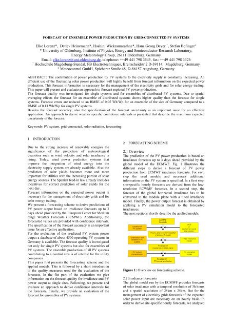
global model of the ECMWF. Fig. 1 illustrates the
different steps to derive a forecast of PV power
production from ECMWF irradiance forecasts. For each
step the used models and necessary additional
information on the PV system is specified. In a first step,
site-specific hourly forecasts are derived from the lowresolution
ECWMF forecasts. In a second step, the
forecast of the global horizontal irradiance has to be
converted to the module plane with a tilted irradiance
model. Finally, the power output forecast is obtained by
applying a PV simulation model to the forecasted
irradiances.
The next sections shortly describe the applied models.
Figure 1: Overview on forecasting scheme.
2.2 Irradiance Forecasts
The global model run by the ECMWF provides forecasts
of solar irradiance with a temporal resolution of 3h hours
and a spatial resolution of 25km x 25km. But for the
management of electricity grids forecasts of the expected
solar power input are necessary on an hourly basis. In
order to derive site-specific hourly forecasts, we analysed

different spatial and temporal interpolation techniques to
refine the ECMWF global model irradiance forecasts. An
optimum adjustment of the temporal resolution was
achieved by combination with a clear sky model to
consider the typical diurnal course of irradiance [1]. As a
second option, a Model Output Statistics (MOS) based
forecasting scheme for solar irradiance using ECMWF
model output described by [2] is evaluated.
2.3 Power Forecast
The incoming irradiance is received on a tilted plane by
most PV systems. Hence, the forecasted horizontal global
irradiance has to be converted according to the
orientation and declination of the modules for processing
in the PV simulation model. Here, the anisotropic-all-sky
model formulated by [3] is used.
In order to derive the power output forecast a robust
simulation model for MPP performance is applied to the
forecasted irradiance on the tilted plane, together with
models of the efficiency characteristics of the inverter
and the different system losses (see. [4]). The model
returns the AC power fed to the grid as function of the
incoming irradiance and the ambient temperature.
Information on the ambient temperature is included as
forecasted values, for the forecasting scheme using MOS.
For the forecasts based on spatial and temporal
interpolation to derive site-specific forecasts, measured
temperature values from nearby meteorological stations
are integrated.
3 QUALITY MEASURES
For the evaluation of forecast quality two error
measures were calculated. The mean values of the
errors:
1 N
BIAS = ∑ ( x forecast i − x
N i=
1
, measured,
i
and the root mean square error:
1 N
2
RMSE = ( x − x ) ,
∑ forecast,
i measured,
i
N i=
1
with x=I for the evaluation of the prediction of the
irradiance I, and x=P=Pac/Pnom for the power forecast.
The normalisation of the ac power output Pac to the
nominal power Pnom of the PV system allows for a better
comparison of different PV systems.
The error measures are calculated for hourly values. Only
day values (xmeasured,i > 0) are considered for the
calculation of BIAS and RMSE.
Also relative values of the error measures (rRMSE,
rBIAS) will be given in the following sections.
Normalization is done with respect to mean ground
measured irradiance or PV power production of the
considered period.
For comparison forecasts based on the assumption of
persistence are evaluated. The irradiance values of the
current day are taken as forecast values for the next days
at the same time. This very simple approach of
forecasting is often used as a reference.
4 ACCURACY OF IRRADIANCE FORECASTS
A comparison of the two proposed approaches for
forecasting was performed by [1] using ground measured
)
,
irradiance data of 18 stations of the German weather
service (DWD) of the years 2003 and 2004. Both
approaches show a similar forecast quality with a rRMSE
of 35%-40% for the first forecast day, and perform much
better than persistence with a rRMSE of about 60%. For
the second and third forecast day errors are only slightly
increasing to an rRMSE of 40% to 45% for the third
forecast day.
For clear sky days the forecast quality is much better.
Best results are achieved with the interpolation technique
combined with a clear sky model, the rRMSE ranges
from 15% for the first forecast day to 20% for the third
forecast day. The respective errors for the MOS system
are about 5%-10% higher.
5 ACCURACY OF POWER FORECAST FOR SINGLE
PV SYSTEMS
For the evaluation of the forecast of the power output a
database of about 4500 operating PV systems in
Germany is available. The forecast for these systems was
processed using the MOS irradiance forecasts. For a
detailed analysis of the forecasts based on the
interpolation technique an ensemble of 11 PV Systems
distributed over an area of 200km x 120km in Southern
Germany was evaluated for April and July 2006 by [5].
These two months with different meteorological
conditions were chosen in order to investigate the
influence of weather conditions on the forecast accuracy.
A validation of the forecast quality for predictions up to
24 hours for the year 2005 using the database of 4500
systems resulted in a RMSE von 0,13 Wh/Wp and a
BIAS of 0,006 Wh/Wp. Fig. 2 shows the accuracy of the
forecast over the year in comparison to persistence. The
figure illustrates the considerable improvement compared
to persistence.
Figure 2: RMSE of hourly PV power production in
Wh/Wp , red: forecast, blue: persistence. The mean value
of all systems is denoted as solid line.
To illustrate the forecast accuracy, time series of
predicted power output in comparison to measured power
output are given for 7 days in April 2006 in Fig. 3, and
for 7 days in July 2006 in Fig. 4 for a system of the
ensemble in Southern Germany. In Fig. 4 also confidence

intervals are displayed that will be further discussed in
the next section.
The figures shows that there is a good agreement
between forecast and measurement for clear sky days
with only minor underestimation of the actual power
output. For cloudy days significant deviations between
forecast and measurement may occur. For overcast
situations a considerable overestimation of the power
output can be observed (see Fig.3, 17 th April).
Furthermore, the strong variation of the power
production for days with variable clouds is not correctly
modelled by the forecast.
Figure 3: Predicted power output compared to
measured power output for seven days in Aril 2006 for a
PV system in Southern Germany.
A quantitative evaluation of the power forecast for the
small ensemble of 11 PV systems resulted in a rRSME of
49% (absolute RMSE=0.12Wh/Wp) for April where
cloudy situations were predominant. For July with
mostly clear sky days for this region a lower rRMSE of
30% (absolute RMSE=0.10 Wh/Wp) is found.
This analysis was complemented with the evaluation of
predictions of irradiance on the tilted plane at the PV
system sites, and an analysis of global horizontal
irradiance forecasts for meteorological stations located in
the same region. The errors of the PV power forecast are
very closely related to the errors of the tilted irradiance
forecast, and the RMSE values are similar. This holds
only if the PV system parameters used for the simulation
have a good quality, which was the case for the evaluated
systems.
The quality of the global horizontal irradiance forecast
with a rRMSE of 44% for April and a rRMSE of 28% for
July is slightly better than the quality of the tilted
irradiance and PV power forecast. Forecast errors are
amplified by conversion of the irradiance on the tilted
plane. But, given correct parameters to characterize the
PV systems, the accuracy of the global horizontal
irradiance forecast is still the determining factor for the
quality of the power forecast.
6 CONFIDENCE INTERVALS
The specification of the forecast accuracy is an important
issue for an effective application of the forecasts.
Therefore, confidence intervals are provided that indicate
the range in which the actual value is expected to appear
with a quantified probability (see illustration in Fig. 4).
To derive the limits of the confidence intervals, a model
for the distribution of the scatter of the actual value
around the forecast is needed. As the range of possible
values is limited by zero and the power output at clear
sky conditions, a natural choice for a respective
distribution model is the beta distribution, already
applied in the context of wind power forecasts [6]. This
model is applied to the small ensemble of 11 Southern
German PV systems.
Figure 4: Predicted power output with confidence
intervals compared to measured power output for seven
days in July 2006 for a PV system in Southern Germany.
Basis for the determination of the confidence intervals is
the knowledge of the situation-specific RMSE of the
forecast. Together with the forecasted value itself it may
define the beta distribution for the expected actual
values.
These specific RMSE values are determined with
dependence on sun elevation and cloud situation
(homogeneous or scatter) using BIAS-corrected forecast
values.
For this analysis only a limited number of measurements
was available. Therefore, only three different classes of
cloud situations are distinguished: clear sky, overcast,
and broken clouds. The characterization of the classes
was based on the mean clear sky index and the standard
deviation of the clear sky index of the forecast field of all
11 PV systems. The clear sky index k* is a measure of
cloudiness, defined as the ratio of global irradiance to
clear sky irradiance.
Given the beta distribution, the limits of the confidence
interval can be directly calculated. Here, we choose a
confidence level of 90%. Fig. 5 shows an example for the
derived confidence intervals for April and sun elevations
between 40 o and 50 o for the three different classes of
cloud situations. The figure illustrates that the confidence
intervals provide a reasonable estimate for the expected
maximum deviation of the measured from the predicted
values. However, a considerable number of values also is
found outside the confidence intervals. A quantitative
evaluation revealed, that only about 80%- 85% of the
measured values are found within the confidence
intervals for each class instead of the expected 90%.
Reasons for this insufficiency may be found in the fact,
that the choice of only two parameters (mean value and
spatial standard deviation the clear sky index k*) to
derive the RMSE data is insufficient, especially taking
into account that the systems analyzed show different

orientations and thus different responses to the cloud
situation. Further analysis has to deal either with system
specific RMSE values or the analysis of ensemble values
and judge about the applicability of the distribution
model on that bases.
Figure 5: Measured power output over predicted power
output with confidence intervals for 11 PV systems in
Southern Germany. The predicted values are BIAS-
corrected for each class separately.
Fig. 5 also illustrates that the different forecast quality
for different meteorological situations is modeled well by
the proposed approach. For clear sky situations the
confidence intervals are chosen very narrow, the forecast
is very reliable. On days with variable clouds large
deviations are to be expected for forecasts with an hourly
resolution for single PV sites.
7 QUALITY OF FORECAST FOR ENSEMBLES OF
PV SYSTEMS
For the management of electricity grids and solar energy
trading the ensemble production of all PV systems
contributing to a control area is relevant.
7.1 Reduction of forecast errors for ensembles of PV
systems
Due to spatial averaging effects the forecast for an
ensemble of distributed systems shows higher accuracy
than the forecast for single systems. Fig. 6 shows a time
series of the power production of the small ensemble of
11 PV systems for seven days in July and the respective
forecasts. Spatial averaging effects cause a smoother
course of the curve of power production than for single
systems (see Fig. 4) and the deviations between forecast
and measurement are smaller.
For the ensemble of 11 PV systems forecast errors are
reduced to a rRMSE of 39% (absolute
RMSE=0.09Wh/Wp) for April and to a rRMSE of 22%
(absolute RMSE=0.06) for July when considering the
power production of the complete ensemble. This
corresponds to an error reduction factor
r=RMSE ensemble/RMSE single of about 0.7.
For the large ensemble of about 4500 PV systems the
evaluation of the ensemble power production forecast
resulted in a RMSE of 0.052Wh/Wp, which corresponds
to an error reduction factor of 0.4 for the complete year
and the region of Germany.
Figure 6: Predicted power output compared to measured
power output for seven days in July 2006 for an
ensemble of PV systems in Southern Germany.
7.2 Correlation of forecast errors
The reduction of errors when considering an ensemble of
PV systems instead of a single system is determined by
the correlation of forecast errors of the systems that are
part of the ensemble.
Figure 7: Correlation coefficient of forecast errors of
two systems over the distance between the systems. The
blue dots represent measured values; the red dots give the
model curve.
The correlation coefficient of the forecast errors of two
systems depends of the distance between the systems, as
illustrated in Fig. 7. Here the correlation coefficient
between two systems is displayed over the distance
between the systems for the large German ensemble. The
dependence of the correlation of the forecast errors on
the distance of two systems can be modelled with an
exponential function. The red line in Fig. 7 shows the
model curve.
This model in combination with a statistical approach to
derive the expected errors of mean values allows for the
estimation of forecasts errors for arbitrary scenarios of
ensembles of PV systems.
7.3 Evaluation of irradiance forecasts for distributed
systems depending on the number of systems and the size
of the region
A detailed analysis on the reduction of forecast errors,
when considering ensembles of distributed systems, was
performed by [5] using measured irradiance data of about

100 meteorological stations in Germany. As the accuracy
of the PV power production forecast is mainly
determined by the accuracy of the irradiance forecasts,
the result of this investigation also gives information
about the quality of PV power forecasts for ensembles of
distributed systems.
[5] investigated the dependency of the forecast quality on
the number of systems and the size of the region, where
the systems are distributed. The distribution of the
meteorological stations and the position and size of
investigated regions is shown in Fig. 8. The evaluation
was performed for the month April and July 2006. For
April, where cloudy situations were predominant, a
RMSE of 160 W/m 2 is found for single stations, when
evaluating the complete ensemble. In July 2006 with
mainly sunny days a considerable smaller RMSE of 110
W/ m 2 is obtained.
Figure 8: Distribution of the meteorological stations and
position and size of the regions used for the evaluation.
As described in the previous sections, for mean
irradiance values for an ensemble of stations the
accuracy is increasing. Fig. 9 shows the rRMSE of the
forecast of the mean irradiance of the ensemble over the
number of considered stations for region 6 (Germany).
The subsets of stations were chosen manually to cover
the complete region with a mostly uniform distribution.
Already for a small number of sites a large reduction of
the forecast errors is achieved. With increasing number
of sites and decreasing distance between the stations the
correlation between the forecast errors is increasing (see
Fig. 7). Consequently, the additional reduction of
forecast errors when adding further sites to the ensemble
is decreasing.
In Fig. 10 the reduction factor RMSE ensemble/RMME single
is displayed over the size of the region. Form each region
20 uniformly distributed stations were chosen to
calculate the reduction factor. For small regions of about
200km x 200km a reduction factor of about 0.6- 0.7 is
found, for a region of the size of Germany a reduction
factor of about 0.4-0.5 is obtained. This in accordance
with the results for the power forecast.
Figure 9: rRMSE of the forecast of the mean irradiance
of an ensemble of stations in dependence on the number
of stations.
Figure 10: Error reduction factor
RMSE ensemble/RMAE single for regions with increasing size
(see Fig. 8).
8 RESULTS AND CONCLUSIONS
An approach to forecast regional PV power production
was presented based on refined ECMWF irradiance
forecasts in combination with a PV simulation model.
The evaluation for hourly irradiance forecasts for single
sites resulted in an overall rRMSE of about 35%-40%.
This leads to a RMSE of about 0,13 Wh/Wp for the
power forecast for single systems. The forecast quality
depends on the meteorological situation: Situations with
inhomogeneous clouds generally are difficult to forecast
and show a lower accuracy than forecasts for clear sky
days.
The specification of the forecast accuracy is an important
issue for an effective application. An approach to derive
weather specific confidence intervals was proposed and
evaluated. The derived confidence intervals provide a
reasonable estimate for the expected maximum deviation

of the measured from the predicted values for different
meteorological situations.
Due to spatial averaging effects the forecast for an
ensemble of distributed systems shows higher quality
than the forecast for single systems. The increase of the
forecast quality essentially depends on the size of the
region, where the PV systems are distributed. For a
region of the size of Germany the forecast errors are
reduced by a factor of about 0.4-0.5. This corresponds to
an absolute RMSE of 0.05 Wh/Wp.
The proposed approach to forecast power production of
PV systems including confidence intervals can contribute
to a successful integration of this fluctuating energy
source to the electricity grid.
8 REFERENCES
[1] Girodo M. (2006): Solarstrahlungsvorhersage auf der
Basis numerischer Wettermodelle, PhD thesis, Oldenburg
University 2006.
[2] Bofinger S., Heilscher G. (2006): Solar electricity
forecast- approaches and first results, 21 th PV
conference, 4 th -8 th September 2006, Dresden.
[3] Klucher, T.M. (1979): Evaluation of models to
predict insolation on tilted surfaces. Solar Energy 23,
111-114.
[4] Drews A., H.G. Beyer, U. Rindelhardt (2007) Quality
of performance assessment of PV plants based on
irradiance maps, submitted to Solar Energy, 4.2007
[5] Wickramarathne H. (2007): Evaluation of Forecast of
Power Production with Distributed PV-Systems, Master
Thesis, Postgraduate Programme Renewable Energy,
Oldenburg University.
[6] Luig A., Bofinger S., Beyer H.G. (2001): Analysis of
confidence intervals for the prediction of the regional
wind power output, 2001 European Wind Energy
Conference, Copenhagen, 2-6. 7.