Denmark Germany - CiteSeerX

THE WIND SPEED PROFILE AT OFFSHORE WIND FARM SITES
1/4
PREPRINT, DEWEK 2002, Wilhelmshaven
Bernhard Lange(1), Søren E. Larsen(2), Jørgen Højstrup (2), Rebecca Barthelmie (2)
(1) Dept. of Energy and Semiconductor Research, Faculty of Physics, University of Oldenburg, D-26111 Oldenburg,
Germany, phone: +49-441-7983927, fax: +49-441-7983326, e-mail: Bernhard.Lange@uni-oldenburg.de
(2) Wind Energy Department, Risø National Laboratory, P.O. Box 49, DK-4000 Roskilde, Denmark
ABSTRACT: Using Monin-Obukhov theory the vertical wind speed profile can be predicted from the wind speed at one
height, when the two parameters Monin-Obukhov length and sea surface roughness are known. The applicability of this
theory for wind power prediction at offshore sites is investigated using data from the measurement program Rødsand in the
Danish Baltic Sea. Different methods to estimate the two parameters are discussed and compared. Significant deviations to
the theory are found for near-neutral and stable conditions, where the measured wind shear is larger than predicted. A
simple correction method to account for this effect has been developed and tested.
As a test application, the wind speed measured at 10 m height is extrapolated to 50 m height and converted to wind turbine
power output. The models for the estimation of the sea surface roughness were found to lead only to small differences,
while for the different methods to derive the Monin-Obukhov length L have an important impact on teh power output
estimations. The simple wind profile correction method, which has been developed, leads to a clear improvement of the
wind speed and power output predictions. For the extrapolation with Monin-Obukhov theory with different L and z0
estimations the prediction error is 5-9%. When the correction is applied, the error reduces to 2-5%. This can be compared
with the result of the WAsP method, which is about 4%.
1 INTRODUCTION
It is expected that an important part of the future
expansion of wind energy utilisation at least in Europe
will come from offshore sites. A reliable prediction of the
wind resource is therefore crucial. This requires the
modelling of the vertical structure of the surface layer
flow, especially the vertical wind speed profile.
The wind speed profile in the atmospheric surface layer is
commonly described by Monin-Obukhov theory (see e.g.
Garratt, 1994). In homogenous and stationary flow
conditions, it predicts a log-linear relation:
⎡ ⎛ ⎞ ⎛ ⎞⎤
= ⎢ ⎜
⎟ − Ψ ⎜ ⎟⎥
⎣ ⎝ ⎠ ⎝ ⎠⎦
∗ u z z
u( z)
ln
(1)
m
κ z0
L
The wind speed u at height z is determined by friction
velocity u *, aerodynamic roughness length z0 and Monin-
Obukhov length L. κ denotes the von Karman constant
(taken as 0.4) and Ψm is a universal stability function.
Glücksburg
Kiel
Germany
50 km
Olpenitz
Boltenhagen
Lübeck
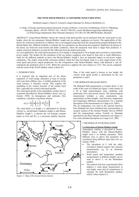
Figure 1: Map of the measurement stations
Tystofte
Denmark
Rødsand
Laage
Thus, if the wind speed is known at one height, the
vertical wind speed profile is determined by the two
parameters z 0 and L.
2 THE RØDSAND MEASURE-MENT
The Rødsand field measurement is located about 11 km
south of the coast of Lolland (see figure 1) and consists of
a 50 m high meteorological mast combined with
underwater wave and current sensors. The meteorological
measurement includes a sonic anemometer, cup
anemometers at three heights, wind direction, temperature
and temperature difference measurements. For a detailed
description of the measurement see Lange et al. (2001).
The air temperature over land in the upwind direction
from Rødsand has been estimated from measurements at
synoptic stations of the German Weather Service (DWD)
and the measurement station Tystofte in Denmark
(operated by the Risø National Laboratory) (see figure 1).
For a more detailed description see Lange et al., 2002.
Barth
3 METHODS OF EXTRAPOLATION
3.1 Derivation of Monin-Obukhov length
Atmospheric stability is described in Monin-
Obukhov theory with the Monin-Obukhov
length scale L as stability parameter. Three
different ways to derive this parameter are
considered using different input data (see e.g.
Garratt, 1994):
• The calculation of L with the eddycorrelation
method requires fast response
measurements, e.g. by an ultrasonic
anemometer.
• Wind speed and temperature gradient
measurements at different heights can be
used to derive L via the Richardson
number.
• The method with least experimental effort
employs a wind speed measurement at
one height, water and air temperatures to
calculate the bulk Richardson number,
which is then related to L.

3.2 Sea surface roughness
Compared to land surfaces the surface roughness of water
is very low. Additionally, it is not constant with wind
speed like for land surfaces, but depends on the wave
field, which in turn is determined by the wind speed, fetch
(distance to coast), etc. It is investigated how different
models to describe the sea surface roughness influence the
prediction of the wind profile. Four models for sea surface
roughness z 0 are considered:
• The simplest ’model’ is the assumption of a constant
roughness, which is e.g. used in the WAsP program
(z 0=0.2 mm) (Mortensen et al., 1993).
• Most commonly used is the Charnock model
(Charnock, 1955), which only depends on friction
velocity.
• Numerous attempts have been made to improve this
description by including more information about the
wave field, e.g. by including wave age (Johnson et
al. 1998) as additional parameters.
• These additional parameters require wave
measurements, which are often not available for
wind power applications. A fetch dependent model
has therefore been developed, where the wave age
has been replaced by utilising an empirical relation
between wave age and fetch (Lange et al., 2001a).
3.3 Comparison with Rødsand measurements
From Monin-Obukhov theory (see eq.(1)) the wind speed
at 50 m height is calculated from the measured 10 m
wind. A deviation ∆ is defined as the ratio between this
predicted and the measured wind speed. This deviation ∆
has been computed for the Rødsand data for all
combinations of the three models to derive the Monin-
Obukhov length L and the four models for the sea surface
roughness.
Systematic deviations are always found for stable
stratification. As example, the deviation ∆ for the gradient
method to derive L is shown in figure 2 with the
Charnock relation used to model z 0. A good agreement is
found in the unstable region (10/L

conduction between land and water the air over land will
often be warmer than the sea surface temperature. The
flow regime that develops in this situation has been
described by several authors. We follow the explanation
given by Csanady (1974):
When warm air is blown over the cold sea, immediately a
stable stratification develops as the air adjacent to the sea
surface will be cooled. Simultaneously an internal
boundary layer develops at the shoreline due to the
roughness and heat flux change. In the case of warm air
advection over cold sea this is a stable internal boundary
layer (SIBL), characterised by low turbulence and
therefore small fluxes and slow growth. The warm air is
cooled from below while the sea surface temperature will
remain almost constant in this process due to the large
heat capacity of water. Eventually, the air close to the sea
surface will have the same temperature as the water and
atmospheric stability will be close to neutral at low
heights. Above the internal boundary layer the air still has
the temperature of the air over land and near the top of the
SIBL an inversion lid has developed with strongly stable
stratification separating these two regions. Thus, while the
stability in the mixed layer is close to neutral, the elevated
stable layer influences the wind speed profile and leads to
a larger wind speed gradient than expected for an ordinary
near neutral condition.
Due to the small fluxes through the inversion lid this flow
regime is a quasi-equilibrium state and can survive for
large distances before eventually the heat flow through the
inversion evens out the difference in potential
temperatures. Eventually the neutral boundary layer is
recovered, which is known from open ocean observations
(Edson and Fairall, 1998).
4.2 Prediction of the inversion height
Csanady (1974) proposes the following expression for the
depth of the mixed layer h in equilibrium conditions:
1 ρ 2
h = A u (2)
∗
g ∆ρ
He estimates the empirical parameter A to 500. Here g is
the gravitational acceleration, ρ the air density, ∆ρ the air
density difference between surface and geostrophic level
u50 meas /u50 pred, Bulk, Charnock
1.40
1.35
1.30
1.25
1.20
1.15
1.10
1.05
1.00
0.95
0.90
10 100 1000 10000
h [m]
Figure 5: Deviation ∆ bin averaged for the estimated
height of inversion layer h (from eq. (2))
3/4
PREPRINT, DEWEK 2002, Wilhelmshaven
at constant pressure and u * the friction velocity. For the
Rødsand measurement the air density at geostrophic level
has been estimated from the measured data at the Rødsand
mast and at the surrounding land stations (see Lange et
al., 2002).
The bin averaged deviation ∆ for situations with long
fetch (>30 km) is shown versus the inversion height h in
Figure 5. The bulk method has been used to determine L
and the Charnock equation for the estimation of z 0. Large
deviations occur for low inversion heights of below 100
m, decreasing rapidly with increasing inversion height
and reaching a constant level at an inversion height of
about 1000 m. This is in accord with the picture that an
inversion height in the order of the boundary layer height
will not lead to changes in the profile.
4.3 Development of a simple correction method
A micrometeorological model to take into account these
effects is not available. Therefore a simple ad hoc
correction method is developed here to investigate the
importance of this effect for wind resource estimations. In
Figure 6 it is shown that the deviation decreases with
increasing height of the inversion layer. It is assumed that
the deviation increases linearly with height. The simplest
correction method is therefore to add a linear correction
term to the wind speed profile of Monin-Obukhov theory
(see eq. 1), which is proportional to the measurement
height z and inversely proportional to the estimated
inversion height h:
⎡ ⎛ ⎞ ⎛ ⎞ ⎤
= ⎢ ⎜
⎟ − Ψ ⎜ ⎟ + ⎥
⎣ ⎝ ⎠ ⎝ ⎠ ⎦
∗ u z z z (3)
u( z)
ln
m c
κ z0
L h
From the Rødsand measurements the correction factor c is
estimated to be about 4.
The effect of this correction on the deviation ∆ is shown
in Figure 6, where ∆ is bin averaged with respect to the
stability parameter 10/L for different methods to derive L.
This can be compared to figure 3, where the same is
shown without correction. It can be seen that the
deviations on the stable side are reduced considerably for
all three methods.
u50 meas /u50 pred
1.20
1.15
1.10
1.05
1.00
Sonic
Gradient
Bulk
0.95
-0.3 -0.2 -0.1 0.0 0.1
10/L
Figure 6: Bin-averaged ratio of measured and predicted
50 m wind speed versus stability parameter 10/L with L
determined by the sonic, gradient and bulk methods and
z 0 with Charnock model; the proposed correction method
for thermal influences is used

Prediction error [%]
-10
-8
-6
-4
-2
0
WAsP
M-O-theory
M-O-theory with correction
Constant
Charnock
Gradient
5 PREDICTIONS OF POWER PRODUCTION
In the context of wind energy utilisation it is important to
know, which impact these different approaches have for
the prediction of the power output of an offshore wind
turbine. This is investigated in an example application:
The power production of an example wind turbine with
hub height 50 m and 1 MW rated power output is
estimated from the wind speed measurement at 10 m
height using the different methods and models described
in the previous sections. The estimated production is than
compared with that obtained by using the measured wind
speed at 50 m height. For this test a 2 year long time
series from Rødsand has been used, where only part of the
measurements are available. Therefore the sonic method
to derive L and the wave age model for z0 could not be
compared.
In Figure 7 the power output prediction error, defined as
(Ppred –Pmeas)/Pmeas, is shown for all extrapolation methods.
The estimated production with wind speed extrapolation
is lower than that using the measured wind speed at hub
height in all cases with errors ranging from 2% to 9%. For
the gradient method to derive L, prediction errors of 7-9%
are found. For the bulk method these are about 6-7%. For
the different sea surface roughness methods it can be seen
that the constant roughness assumption and the Charnock
relation lead to almost equal results. The fetch model
shows a slightly (about 1%) larger error. Using the
correction method for the profile, the errors are reduced
by about 4%. The results are also compared with the error
of the WAsP method, which is about 4%.
6 CONCLUSION
Wind resource estimation at offshore sites is more
complex than often believed. Not only the variable sea
surface roughness, the determination of the atmospheric
stability and the growth of the internal boundary layer
complicate the situation, but also the land-sea
discontinuity can lead to a special flow situation far
offshore. In this flow regime the wind speed increases
more rapidly with height than predicted by Monin-
Constant
Bulk
Figure 7: Error in power output prediction (Pmeas-
Ppred)/Pmeas of an example turbine for the 2 year long
Rødsand data set; different methods to extrapolate the
wind speed measurement at 10 m height to 50 m are used
(see text); the result with the WAsP method is also shown
Fetch
Charnock
Fetch
4/4
PREPRINT, DEWEK 2002, Wilhelmshaven
Obukhov theory. It should be noted that these deviations,
although caused by the coastal discontinuity, where found
far offshore for fetches of 30 to 100 km.
Currently these conclusions can be drawn for the site
Rødsand only and need to be validated with other
measurements. But from this example it can be seen that
the flow modification in conditions of warm air advection
from land plays an important role in the flow regime at
offshore sites. At Rødsand this is the dominating
uncertainty in the description of the wind conditions. We
expect that a better understanding of this effect is a
prerequisite for future improvements in the description of
the wind regime over the coastal zone.
To improve the wind resource estimation for offshore
sites, a model for the flow regime in conditions of warm
air advection from land over sea is needed. The simple
correction method introduced in this paper is intended to
show the importance of the effect, but can not be used as a
general model of the flow regime. Further development
with data from additional sites is needed. Until such a
model is available, measurements at or close to hub height
are necessary for an accurate estimation of the wind
resource of an offshore location.
ACKNOWLEDGEMENT
The Rødsand measurement program was funded by:
JOULE program of the EU (JOU2-CT93-0325), Office of
naval research (N00014-93-1-0360), Danish Energistyrelsen
(UVE J.nr. 51171/96-0040) and ELKRAFT. The
technical support team at Risø and Sydfalster-El are
acknowledged for their contribution to the data collection.
REFERENCES
Charnock, H, 1955: Wind stress over a water surface.
Quart. J. Roy. Meteor. Soc, 81, 639-640.
Csanady GT, 1974: Equilibrium theory of the
planetary boundary layer with an inversion lid. Boundary-
Layer Meteorol., 6, 63-79.
Edson JB. Fairall CW, 1998: Similarity relationships
in the marine atmospheric surface layer for terms in the
TKE and scalar variance budgets. J. Atmos. Sci., 55,
2311-2328.
Garratt JR, 1994: The atmospheric boundary layer.
Cambridge, Cambridge University Press.
Johnson HK, Højstrup J, Vested HJ, Larsen SE, 1998:
On the Dependence of Sea Surface Roughness on Wind
Waves. J. Phys. Oceanogr.. 28, 1702-1716.
Lange B, Barthelmie RJ and Højstrup J, 2001:
Description of the Rødsand field measurement. Report
Risø-R-1268. Risø National Laboratory, DK-4000
Roskilde, Denmark.
Lange B., Højstrup J, Larsen SE, Barthelmie RJ,
2001a: A fetch dependent model of sea surface roughness
for offshore wind power utilisation. European Wind
Energy Conference, Copenhagen, Denmark.
Lange B, Larsen S, Højstrup J, Barthelmie R, 2002:
The influence of thermal effects on the wind speed profile
of the coastal marine boundary layer. submitted to
Boundary-Layer Meteorol.
Mortensen NG, Landberg L, Troen I, Petersen EL,
1993: Wind Analysis and Application Program (WASP),
User’s Guide. Risoe-I-666(EN) (v.2), Risø National
Laboratory, Denmark; 133 pp.