Problems - OpenTrack

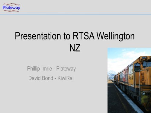
Presentation to RTSA Wellington 

NZ 

Phillip Imrie - Plateway 

David Bond - KiwiRail

Corporate Background 

Plateway Pty Ltd 

Sydney Office 

6/3 Sutherland Street 

Clyde NSW 2142 

Australia 

Phone: +61 2 9637 5830 

Fax: +61 2 9637 6350

Global and Local Partners 

• Plateway works in close collaboration with several leading 

local and global partners 

– SMA and Partners Zurich 

– OpenTrack GmbH 

– Savannah Simulations 

– IFB Dresden 

– LIFT Trieste

Corporate Background 

• Plateway has worked throughout Australia and New 

Zealand. 

• Plateway’s core business has grown from a railway 

infrastructure management capability focusing on process 

redesign. 

• Plateway has since expanded to a much wider total rail 

systems capability. 

• Clients include rail operators, network owners and 

increasingly, rail customers.

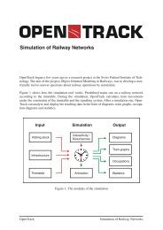
Why Simulate? 

Simulation Tools 

• Computer simulation allows a virtual reconstruction of 

complex systems both natural and man made. 

• Takes into account the combined effect of all known 

variables and uncertainties. 

• Very cheap means of obtaining experience. 

• Unexpected problems and conflicts within a system can be 

detected and solved.

Why Simulate? 

Simulation Tools 

• Test Sensitivity of System Performance to inputs such as 

rollingstock, passenger patronage, freight volume, 

infrastructure configuration (track, signals), system 

reliability, access policy. 

• Obtain stakeholder buy in. 

• Communicate awareness of system drivers. 

• Inputs to downstream processes.

Benefits of Simulation 

• More control of modelling parameters. 

• Reduces risk. 

• Reduce project lengths. 

• Visual representation which flowcharts and spreadsheets do 

not have. 

• Reduce design errors in the preliminary stages. 

• Can help decide project feasibility. 

• All benefits can reduce costs.

Types of Computer Simulation 

Simulation Features 

Dynamic simulations Models changes in a system in response to a 

defined input signal. 

Stochastic models Uses random number generators to model chance 

or random events. 

Discrete event simulation Manages events in time- the computer simulates a 

queue of events in the order in which they occur. 

Continuous dynamic simulation Solves differential equations and uses the solution 

to change the simulation. 

Source: Wikipedia

Dynamic Simulation 

A dynamic simulation could be achieved by altering train 

arrival times to see which combinations may cause a problem. 

Problems 

• There may be combinations that can either not occur or are 

extremely likely to occur in reality.

Locations 

Reading Train Graphs 

Time 

Slope of graph line shows train speed- the steeper the line the quicker the train

Dynamic Simulation

Dynamic Simulation

Stochastic models 

Could be achieved by describing train run times as a statistical 

distribution. 


• The statistical distribution does not calculate actual train 

performance. 

• Maybe incorrect relationships between cause and effect. 

• Major problems if outliers are not analysed and treated 

correctly.

Benefits of Stochastic Models 

Stochastic Models 

• Modeling should be based on a range of outcomes. 

• On time running is defined relative to that range i.e. about 

threading the train path through a series of nodes within an 

allowable band rather than an absolute value. 

• Measure the expected reliability of a timetable change.

Stochastic models

Discrete Event Simulation 

Discrete event simulations are generally based on the 

response of a service based system (say the operation of a 

bank) to a defined event such as a queue. 


• The cause of queuing is not identified.

Continuous Dynamic Simulation 

Uses equations which describe the physical processes 

involved to generate a simulation. 


• Complicated code required which solves multiple ordinary 

differential equations. Requires a large amount of 

computing power.

OpenTrack Network Simulator

OpenTrack Users 

Railway/metro companies, railway administrations Consultancies 

Universities and research institutes Railway supply industry / maglev industry

May 2012 

OpenTrack Users 

• 248 OpenTrack licenses have been sold to 164 

Companies and Institutes in 33 countries. 

September 2010 

• OpenTrack had issued 150 licences to 80 different 

holders within 22 countries.

OpenTrack Calculation Algorithm 

The calculation engine in OpenTrack uses the equations of 

motion to calculate each trains acceleration, speed and 

position at a given point in time. 

Force = mass x acceleration. 

To move a train the power unit has to apply a net tractive effort 

to overcome the resisting forces. 

So the acceleration becomes: 

Acceleration = Net tractive effort 

mass


The “resisting” forces 

considered in the 

OpenTrack calculation 

include: 

• power unit losses 

• rolling resistance 

• the track gradient 

over the train length 

• the track curvature 

over the train length

To perform the calculation 

OpenTrack needs a reference 

set of data. This includes: 

Traction unit characteristics 

including a speed vs. tractive 

effort curve. 

Environmental conditions, how 

slippery the rail is. 

OpenTrack Input Data

Assumed train braking performance. 

OpenTrack Input Data 

• Increasingly modern systems blend air and electric 

(dynamic) braking. 

• Blending is computer controlled and dependent on 

environmental conditions as well as individual driving style.


• Railway curves, grades and line speeds.


• Signaling layouts and interlocking functionality. 

Source: RailCorp Network Documentation


Once the net force available for traction has been calculated 

the computer apples differential calculus to the acceleration 

using the Euler method to calculate the speed of the train and 

then again to calculate the trains position. 

Source: OpenTrack Manual


The Euler method is an approximation but computers cannot 

solve differential equations. 

The accuracy of the approximation improves with decreasing 

the time interval used in the calculation.


• The acceleration and speed are also adjusted as a result of 

the signaling system inputs. 

• Other defined “events” which are triggered by distance may 

include station stops, changes in train loading and direction. 

• Once the computer has finished the calculations for each 

time interval the computer starts again for the next 

increment. 

• The method uncorrected will generally produce the “best 

performance” possible. For use in practical applications this 

is always down rated.

Traction Power Supply Simulation 

The basic electrical Ohms law relationship is a major factor in 

deciding the parameters for the chosen system. 

Voltage (U) = current (I) x Impedance (Z) 

The losses in the conductors can be given by P= I 2 Z 

So the higher the voltage, the lower the current and the lower the 

system losses.


In an AC system the impedance to the flow of current is a 

function of: 

• The resistance. 

• Magnetic coupling between the supply and return side 

conductors. 

• Capacitive coupling is a component of impedance but not a 

major influence in traction supply systems. It does however 

generate interference.


Resistance to the flow of current is a function of: 

• Conductor size. 

• Conductor material. 

• Conductor temperature. 

• Conductor length - in a traction supply the distance of the 

train to the supply point. 

• Component wear (of contact wire and rails)


Why simulate the traction power supply? 

• To determine the line voltage at the pantograph and the 

resulting impact on train performance. 

• To determine the influence of the network structure on 

electrical load distribution. 

• To size equipment such as cable, transformers, rectifiers 

• Some energy suppliers have constraints on the ability of the 

network to cope with regenerated energy under different 

network switching conditions.


The power supply system influences the resultant energy 

consumption and costs as well as train performance. 

Simulation of these dynamic processes enables: 

• Energy consumption analysis and prognosis. 

• Design and rating verification of the electrical installations. 

• Electromagnetic field studies.


Energy consumption simulation for electrical railway 

systems is a factor of: 

• Whether the train is powering or braking. 

• The throttle setting and required traction power. 

• The position of the trains within the network. 

• The configuration and capability of the power supply system. 

All of this information is needed at exactly the same time.


Older simulation products compromised on: 

• the complexity of the rail operation (only able to simulate a 

small number of trains). 

• the detail of traction unit performance under degraded line 

conditions and feedback into the simulation. 

• the detail of the electrical network.


ATM 

Advanced Train Module 

Locomotives adjust performance in 

response to available power supply 

Propulsion Technology 

Railway Operation Simulation 

Uses calculus to calculate the position, speed, acceleration and resulting 

power demand of every train in the network 

“Co-Simulation” 

Interaction 

PSC Power Supply Calculation 

Uses calculus to solve Ohm’s Law to 

calculate current, voltage, 

resistance. 

Power Supply System

Structure of OPN

Traction Power Supply Simulation

Data Input 


• Electrical network structure (feeding sections, feeding 

points, switch state) in congruence to the track topology. 

• Electrical characteristics of the feeding power grid. 

• Electrical characteristics of the substations. 

• Electrical characteristics of the conductors (cables, 

Catenary wires, tracks, rails). 

• Electrical characteristics rail-to-earth.

Data Input 


• Modelling of additional power consumers (e.g. switch 

heaters). 

• Loading capacity (conductors, converters, transformers). 

• Protection settings.





• Developed by IFB Dresden 

tool development 

to work with a commercial rail network simulator. 

• Initial deployment on high speed network in the Netherlands 

• Then used to simulate the operation of the Zurich tramways 

and trolley bus system.


tool development 

• License sold to the Fourth Railway Survey and Design 

Institute in China. 

• Used for design verification for High Speed and Metro 

projects.

Cleveland Line Proof of Concept 

• QR required comfort that the power supply simulation would 

produce data which could be used with confidence for future 

network design and analysis. 

• Proof of Concept involved a series of instrumented single 

train runs and logging the performance of a traction sub 

station over five days and comparing the measured results 

with the simulated results. 

• First time this has been done for a 25 kV AC urban rail 

network.


• Measured voltage at each end and at Lytton Junction 

substation. 

• The energy consumption was measured at the feeding 

location.


Source: http://www.queenslandrail.com.au/NetworkServices/DownloadsandRailSystemMaps/SEQ/Pages/ClevelandLine.aspx 

• Part of the Brisbane suburban railway network. 

• Runs east from Park Road station on the south of the river for 

32 km to Cleveland. 

• Line contains single and double sections. 

• Fifteen peak hour services every weekday.

Potential Variables 

• Driving style. 


• Interpretation of running rules and driver’s instruction 

manual. 

• Use of different rollingstock types each with different 

performance characteristics. 

• Daily timetable variations. 

• System feeding.

Cleveland Line Proof of Concept

Single Train Run Results

Issues 

Single Train Run Results 

• Sometimes the simulation output and measurement are 

calculating different things. 

• The trains position had to be adjusted based on the AWS 

magnets as the traction / braking systems included 

controlled wheel slip which reduced odometer accuracy. 

• The difficulty in simulating the blended braking is apparent. 

• Even with a substantial performance derating, the 

simulation powers and brakes far harder than the human 

driver.


• To enable the simulated and measured results to be 

compared the timetable had to be adjusted to account for 

actual train running. 

• The global performance factor was adjusted to provide an 

average of how the trains were being driven.

Actual Timetable – Tue 31 st Jan 

To show the way that the OpenTrack performance change from 97% to 90% 

Impacts on the simulation; for the Tuesday operation both diagrams are presented

Actual Timetable – Tue 31 st Jan 

Performance Setting 97%

Actual Timetable – Tue 31 

Performance Setting 90% 

st Jan

Network Simulation Results

Results 


• Extremely good correlation between single train simulations 

and measured values. 

• The morning peak simulations were within the acceptance 

criteria. 

• The results illustrated a very different electrical performance 

of assets at each end of the line.

For further details please see: 

http://www.openpowernet.de 

Further Details 

http://www.opentrack.ch/opentrack/opentrack_e/opentrack_e.html 

http://www.plateway.com.au/

Problems - OpenTrack

You also want an ePaper? Increase the reach of your titles

Delete template?

Save as template?