SparQ: A Toolbox for Qualitative Spatial Representation and ...

SparQ: A Toolbox for Qualitative Spatial
Representation and Reasoning
Frank Dylla, Lutz Frommberger, Jan Oliver Wallgrün, and Diedrich Wolter
SFB/TR 8 Spatial Cognition
Universität Bremen
Bibliothekstr. 1, 28359 Bremen, Germany
{dylla,lutz,wallgruen,dwolter}@sfbtr8.uni-bremen.de
Abstract. A multitude of calculi for qualitative spatial reasoning (QSR)
has been proposed during the last two decades. The number of practical
applications that make use of QSR techniques is, however, comparatively
small. One reason for this may be seen in the difficulty for people from
outside the field to incorporate the required reasoning techniques into
their software. Sometimes, proposed calculi are only partially specified
and implementations are rarely available. With the SparQ toolbox presented
in this text, we seek to improve this situation by making common
calculi and standard reasoning techniques accessible in a way that allows
for easy integration into applications. We hope to turn this into a community
effort and encourage researchers to incorporate their calculi into
SparQ. This text provides an overview on SparQ and its utilization.
1 Introduction
Qualitative spatial reasoning (QSR) is an established field of research pursued by
investigators from many disciplines including geography, philosophy, computer
science, and AI [1]. The general goal is to model commonsense knowledge and
reasoning about space as efficient representation and reasoning mechanisms that
are still expressive enough to solve a given task.
Following the approach taken in Allen’s seminal paper on qualitative temporal
reasoning [2], QSR is typically realized in form of calculi over sets of spatial
relations (like ‘left-of’ or ‘north-of’). These are called qualitative spatial calculi.
A multitude of spatial calculi has been proposed during the last two decades, focusing
on different aspects of space (mereotopology, orientation, distance, etc.)
and dealing with different kinds of objects (points, line segments, extended objects,
etc.). Two main research directions in QSR are mereotopological reasoning
about regions [3,4,5] and reasoning about positional information (distance and
orientation) of point objects [6,7,8,9,10] or line segments [11,12,13].
Despite this huge variety of qualitative spatial calculi, the amount of applications
employing qualitative spatial reasoning techniques is comparatively small.
We believe that important reasons for this are the following: Choosing the
right calculus for a particular application is a challenging task, especially for people
not familiar with QSR. Calculi are often only partially specified and usually

no implementation is made available—if the calculus is implemented at all and
not only investigated theoretically. As a result, it is not possible to “quickly” evaluate
how different calculi perform in practice. Even if an application developer
has decided on a particular calculus, he has to invest serious efforts to include
the calculus and required reasoning techniques into the application. For many
calculi this is a time-consuming and error-prone process (e.g. involving writing
down huge composition tables, which are often not even completely specified in
the literature).
Overall, we are convinced that the QSR community should strive for making
the fruits of its work available to the public in a homogeneous framework.
We have thus started the development of a qualitative spatial reasoning toolbox
called SparQ 1 that aims at supporting the most common tasks—qualification,
computing with relations, constraint-based reasoning, etc. (cp. section 3)—for an
extensible set of spatial calculi. A complementary approach aiming at the specification
and investigation of the interrelations between calculi has been described
in [14]. Here, the calculi are defined in the algebraic specification language CASL.
In contrast, our focus is on providing an implementation of QSR techniques that
is tailored towards the needs of application developers. In its current version,
SparQ mainly concentrates on calculi from the area of reasoning about the orientation
of point objects or line segments. However, specifying and adding new
calculi is in most cases very simple. We hope to turn this into a community effort,
encouraging researchers from other groups to incorporate their own calculi.
In this text, we describe SparQ and its utilization. The current version of
SparQ and further documentation will be made available at the SparQ homepage
2 . The next section briefly recapitulates the relevant terms concerning QSR
and spatial calculi as needed for the remainder of the text. In section 3, we describe
the services provided by SparQ. Section 4 explains how new calculi can be
be incorporated into SparQ and section 5 describes how SparQ can be integrated
into own applications.
2 Reasoning with qualitative spatial relations
A qualitative spatial calculus defines operations on a finite set R of spatial
relations. The spatial relations are defined over a particular set of spatial objects,
the domain D (e.g. points in the plane, oriented line segments, etc.). While
a binary calculus deals with binary relations R ⊆ D × D, a ternary calculus
operates with ternary relations R ⊆ D × D × D.
A spatial calculus establishes a set of typically jointly exhaustive and pairwise
disjoint (JEPD) base relations BR. The set R of all relations considered by the
calculus contains at least the base relations, the empty relation ∅, the universal
relation U, and the identity relation Id; the set R should be closed under the
1 Spatial Reasoning done Qualitatively
2 http://www.sfbtr8.uni-bremen.de/project/r3/sparq/

operations defined in the following. Typically, the powerset of the base relations
2 BR is chosen for R. 3
As the relations are subsets of tuples from the same Cartesian product, the
set operations union, intersection, and complement can be directly applied:
Union: R ∪ S = { x | x ∈ R ∨ x ∈ S }
Intersection: R ∩ S = { x | x ∈ R ∧ x ∈ S }
Complement: R = U \ R = { x | x ∈ U ∧ x �∈ R }
where R and S are both n-ary relations on D. The other operations depend on
the arity of the calculus.
2.1 Operations for binary calculi
For binary calculi, two other important operations are required:
Converse: R � = { (y, x) | (x, y) ∈ R }
(Strong) composition: R ◦ S = { (x, z) | ∃y ∈ D : ((x, y) ∈ R ∧ (y, z) ∈ S) }
For some calculi no finite set of relations exists that includes the base relations
and is closed under composition as defined above. In this case, a weak
composition is defined instead that takes the union of all base relations that have
a non-empty intersection with the result of the strong composition:
Weak composition: R ◦weak S = { d | T ∈ BR ∧ d ∈ T ∧ T ∩ (R ◦ S) �= ∅ }
2.2 Operations for ternary calculi
While there is only one possibility to permute the two objects of a binary relation
which leads to the converse operation, there exist 5 such permutations for the
three objects of a ternary relation. This results in the following operations 4 [15]:
Inverse: INV(R) = { (y, x, z) | (x, y, z) ∈ R }
Short cut: SC(R) = { (x, z, y) | (x, y, z) ∈ R }
Inverse short cut: SCI(R) = { (z, x, y) | (x, y, z) ∈ R }
Homing: HM(R) = { (y, z, x) | (x, y, z) ∈ R }
Inverse homing: HMI(R) = { (z, y, x) | (x, y, z) ∈ R }
Composition for ternary calculi is defined accordingly to the binary case:
(Strong) comp.: R ◦ S = { (w, x, z) | ∃y ∈ D : ((w, x, y) ∈ R ∧ (x, y, z) ∈ S) }
Other ways of composing two ternary relations can be expressed as a combination
of the unary permutation operations and the composition [16] and thus do
not have to be defined separately. The definition of weak composition is identical
to the binary case.
3 Unions of relations correspond to disjunction of relational constraints and thus we
will often simply speak of disjunctions of relations as well and write them as sets
{R1, ..., Rn}.
4 It is not needed to specify all these operations as some can be expressed by others.

2.3 Constraint reasoning with spatial calculi
Spatial calculi are often used to formulate constraints about the spatial configurations
of a set of objects from the domain of the calculus as a constraint
satisfaction problem (CSP): Such a spatial constraint satisfaction problem then
consists of a set of variables X1, ..., Xn (one for each spatial object) and a set of
constraints C1, ..., Cm (relations from the calculus). Each variable Xi can take
values from the domain of the utilized calculus. CSPs are often visualized as
constraint networks which are graphs with nodes corresponding to the variables
and arcs corresponding to constraints. A CSP is consistent, if an assignment
for all variables to values of the domain can be found, that satisfies all the constraints.
Spatial CSPs usually have infinite domains and thus backtracking over
the domains can not be used to determine global consistency.
Besides global consistency, weaker forms of consistency called local consistencies
are of interest in QSR. On the one hand, they can be employed as a forward
checking technique reducing the CSP to a smaller equivalent one (one that has
the same set of solutions). Furthermore, in some cases they can be proven to
be not only necessary but also sufficient for global consistency for the set R of
relations of a given calculus. If this is only the case for a certain subset S of R
and this subset exhaustively splits R (which means that every relation from R
can be expressed as a disjunction of relations from S), this at least allows to formulate
a backtracking algorithm to determine global consistency by recursively
splitting the constraints and using the local consistency as a decision procedure
for the resulting CSPs with constraints from S [17].
One important form of local consistency is path-consistency which (in binary
CSPs) means that for every triple of variables each consistent evaluation of the
first two variables can be extended to the third variable in such a way that all
constraints are satisfied. Path-consistency can be enforced syntactically based on
the composition operation (for instance with the algorithm by van Beek [18]) in
O(n 3 ) time where n is the number of variables. However, this syntactic procedure
does not necessarily yield the correct result with respect to path-consistency as
defined above. Whether this is the case or not needs be investigated for each
individual calculus.
2.4 Supported calculi
The calculi currently included in SparQ are the FlipFlop Calculus (FFC) [8]
with the LR refinement described in [19], the Single Cross Calculus (SCC) and
Double Cross Calculus (DCC) [6], the coarse-grained variant of the Dipole Relation
Algebra (DRAc) [11,12], the Oriented Point Relation Algebra OPRAm
[9], as well as RCC-5 and RCC-8 5 [3]. An overview is given in Table 1 where
the calculi are classified according to their arity (binary, ternary), their domain
(points, oriented points, line segments, regions), and the aspect of space modeled
(orientation, distance, mereotopology). As can be seen, mainly calculi for
5 Currently only the relational specification is available for RCC, but no qualifier.

arity domain aspect of space
Calculus binary ternary point or. point line seg. region orient. dist. mereot.
FFC/LR
SCC
DCC
DRAc
OPRAm
RCC-5/8
√
√
√
√
√
√
√
√
√
√
√
√
√
√
√
√
√
√
Table 1. The calculi currently included in SparQ
s l e
A B
A
r
B
C
C
(a) (b)
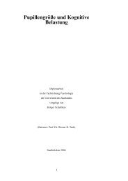
Fig. 1. Illustration of DRAc: (a) The FlipFlop relations used to define Dipole relations.
(b) A dipole configuration: dAB rlll dCD in DRAc.
reasoning about orientation have been incorporated so far, but calculi dealing
with other kinds of base objects or dealing with other aspects of space can be
integrated just as easily. We briefly describe DRAc as it will be used in the
examples in the remainder of this text.
DRAc A dipole is an oriented line segment as e.g. determined by a start and an
end point. We will write dAB for a dipole defined by start point A and end point
B. The idea of using dipoles was first introduced by Schlieder [11] and extended in
[12]. The coarse-grained dipole calculus variant (DRAc) describes the orientation
relation between two dipoles dAB and dCD with the preliminary of A, B, C, and
D being in general position, i.e., no three disjoint points are collinear. Each base
relation is a 4-tuple (r1, r2, r3, r4) of FlipFlop relations relating one point from
one of the dipoles with the other dipole. r1 describes the relation of C with
respect to the dipole dAB, r2 of D with respect to dAB, r3 of A with respect to
dCD, and r4 of B with respect to dCD. The distinguished FlipFlop relations are
left, right, start, and end (see Figure 1 (a)). Dipole relations are usually written
without commas and parentheses, e.g. rrll. Thus, the example in Figure 1 (b)
shows the relation dAB rlll dCD.
3 SparQ
SparQ consists of a set of modules that provide different services required for
QSR that will be explained below. These modules are glued together by a central
script that can either be used directly from the console or included into own
applications via TCP/IP streams in a server/client fashion (see section 5).
D

The general syntax for using the SparQ main script is as follows:
$ ./sparq
Example:
$ ./sparq compute-relation dra-24 complement "(lrll llrr)"
where ‘compute-relation’ is the name of the module to be utilized, in this case the
module for conducting operations on relations, ‘dra-24’ is the SparQ identifier
for the dipole calculus DRAc, and the rest are module specific parameters, here
the name of the operation that should be conducted (complement) and a string
parameter representing the disjunction of the two dipole base relations lrll and
llrr 6 . The example call thus computes the complement of the disjunction of these
two relations. SparQ provides the following modules:
qualify transforms a quantitative geometric description of a spatial configuration
into a qualitative description based on one of the supported calculi
compute-relation applies the operations defined in the calculi specifications
(intersection, union, complement, converse, composition, etc.) to a set of
spatial relations
constraint-reasoning performs computations on constraint networks
Further modules are planned as future extensions. This comprises a quantification
module for turning qualitative scene descriptions back into quantitative
geometric descriptions and a module for neighborhood-based spatial reasoning.
In the following section we will take a closer look at the three existent modules.
3.1 Qualification and scene descriptions
The purpose of the qualify module is to turn a quantitative geometric scene
description into a qualitative scene description composed of base relations from
a particular calculus. The calculus is specified via the calculus identifier that
is passed with the call to SparQ. Qualification is required for applications in
which we want to perform qualitative computations over objects whose geometric
parameters are known.
The qualify module reads a quantitative scene description and generates a
qualitative description. A quantitative scene description is a space-separated list
of base object descriptions enclosed in parentheses. Each base object description
is a tuple consisting of an object identifier and object parameters that depend
on the type of the object. For instance, let us say we are working with dipoles
which are oriented line segments. The object description of a dipole is of the
form ‘(name xs ys xe ye)’, where name is the identifier of this particular dipole
object and the rest are the coordinates of start and end point of the dipole. Let
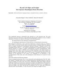
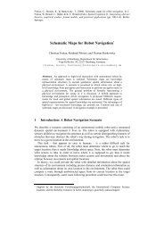
us consider the example in Figure 2 which shows three dipoles A, B, and C. The
quantitative scene description for this situation would be:
6 Disjunctions of base relations are always represented as a space-separated list of the
base relations enclosed in parentheses in SparQ.

5
A
y
0
C
Fig. 2. An example configuration of three dipoles.
( (A -2 0 8 0) (B 7 -2 2 5) (C 1 -1 4.5 4.5) )
The qualify module has one module specific parameter:
mode This parameter controls which relations are included into the qualitative
scene description: If the parameter is ‘all’, the relation between every object
and every other object will be included. If it is ‘first2all’ only the relations
between the first and all other objects are computed.
The resulting qualitative scene description is a space-separated list of relation
tuples enclosed in parentheses. A relation tuple consists of an object identifier
followed by a relation name and another object identifier, meaning that the first
object stands in this particular relation with the second object. The command
to produce the qualitative scene description followed by the result is 7 :
$ ./sparq qualify dra-24 all
$ ( (A -2 0 8 0) (B 7 -2 2 5) (C 1 -1 4.5 4.5) )
> ( (A rllr B) (A rllr C) (B lrrl C) )
3.2 Computing with relations
The compute-relation module allows to compute with the operations defined in
the calculus specification. The module specific parameters are the operation that
should be conducted and one or more input relations depending on the arity of
the operation. Let us say we want to compute the converse of the llrl dipole
relation. The corresponding call to SparQ and the result are:
$ ./sparq compute-relation dra-24 converse llrl
> (rlll)
The result is always a list of relations as operations often yield a disjunction
of base relations. The composition of two relations requires one more relation as
parameter because it is a binary operation, e.g.:
$ ./sparq compute-relation dra-24 composition llrr rllr
> (lrrr llrr rlrr slsr lllr rllr rlll ells llll lrll)
7 In all the examples, input lines start with ‘$’. Output of SparQ is marked with ‘>’.
5
B
x

Here the result is a disjunction of 10 base relations. It is also possible to have
disjunctions of base relations as input parameters. For instance, the following
call computes the intersection of two disjunctions:
$ ./sparq compute-relation dra-24 intersection "(rrrr rrll rllr)"
"(llll rrll)"
> (rrll)
3.3 Constraint reasoning
The constraint-reasoning module reads a description of a constraint network—
which is a qualitative scene description that may include disjunctions and may
be inconsistent and/or underspecified—and performs a particular kind of consistency
check 8 . Which type of consistency check is executed depends on the first
module specific parameter:
action The two actions currently provided are ‘path-consistency’ and ‘scenarioconsistency’
and determine which kind of consistency check is performed.
The action ‘path-consistency’ causes the module to enforce path-consistency on
the constraint network using van Beek’s algorithm [18] or detect the inconsistency
of the network in the process. We could for instance check if the scene
description generated by the qualify module in section 3.1 is path-consistent
which of course it is. To make it slightly more interesting we add the base relation
ells to the constraint between A and C resulting in a constraint network
that is not path-consistent:
$ ./sparq constraint-reasoning dra-24 path-consistency
$ ( (A rllr B) (A (ells rllr) C) (B lrrl C) )
> Modified network.
> ( (B (lrrl) C) (A (rllr) C) (A (rllr) B) )
The result is a path-consistent constraint network in which ells has been removed.
The output ‘Modified network’ indicates that the original network was not pathconsistent
and had to be changed. Otherwise, the result would have started with
‘Unmodified network’. In the next example we remove the relation rllr from the
disjunction between A and C. This results in a constraint network that cannot
be made path-consistent which implies that it is not globally consistent.
$ ./sparq constraint-reasoning dra-24 path-consistency
$ ( (A rllr B) (A ells C) (B lrrl C) )
> Not consistent.
> ( (B (lrrl) C) (A () C) (A (rllr) B) )
8 The constraint-reasoning module also provides some basic actions to manipulate
constraint networks that are not further explained in this text. One example is the
‘merge’ operation that is used in the example in section 5.

SparQ correctly determines that the network is inconsistent and returns the
constraint network in the state in which the inconsistency showed up (indicated
by the empty relation () between A and C).
If ‘scenario-consistency’ is provided as argument, the constraint-reasoning
module checks if a path-consistent scenario exists for the given network. It uses
a backtracking algorithm to generate all possible scenarios and checks them
for path-consistency as described above. A second module specific parameter
determines what is returned as the result of the search:
return This parameter determines what is returned in case of a constraint network
for which path-consistent scenarios can be found. It can take the values
‘first’ which returns the first path-consistent scenario, ‘all’ which returns all
path-consistent scenarios, and ‘interactive’ which returns one solution and
allows to ask for the next solution until all solutions have been iterated.
Path-consistency is also used as a forward-checking method during the search
to make it more efficient. For certain calculi, the existence of a path-consistent
scenario implies global consistency. However, this again has to be investigated
for each calculus. As a future extension it is planned to allow to specify splitting
subsets of a calculus for which path-consistency implies global consistency
and provide a variant of the backtracking algorithm that decides global consistency
by searching for path-consistent instantiations that only contain relations
from the splitting subset. In the following example, we use ‘first’ as additional
parameter so that only the first solution found is returned:
$ ./sparq constraint-reasoning dra-24 scenario-consistency first
$ ( (A rele C) (A ells B) (C errs B) (D srsl C) (A rser D) (D rrrl B) )
> ( (B (rlrr) D) (C (slsr) D) (C (errs) B) (A (rser) D) (A (ells) B)
(A (rele) C) )
In case of an inconsistent constraint network, SparQ returns ‘Not consistent.’
4 Specifying calculi in SparQ
For most calculi it should be rather easy to include them into SparQ. The main
thing is to provide the calculus specification. Listing 1.1 shows an extract of
the definition of a simple exemplary calculus for reasoning about distances between
three point objects distinguishing the three relations ‘closer’, ‘farther’, and
‘same’. The specification is done in Lisp-like syntax.
The arity of the calculus, the base relations, the identity relation and the
different operations have to be specified, using lists enclosed in parentheses (e.g.
when an operation returns a disjunction of base relations). In this example, the
inverse operation applied to ‘same’ yields ‘same’ and composing ‘closer’ and
‘same’ results in the universal relation written as the disjunction of all base
relations. Some operations like homing and short cut operations are left out in
the example (cmp. section 2.2).

( def-calculus " Relative distance calculus ( reldistcalculus )"
: arity : ternary
: base-relations ( same closer farther )
: identity-relation same
5 : inverse-operation (( same same )
( closer closer )
( farther farther ))
: composition-operation (( same same ( same closer farther ))
( same closer ( same closer farther ))
10 ( same farther ( same closer farther ))
( closer same ( same closer farther ))
( closer closer ( same closer farther ))
( closer farther ( same closer farther ))
[...]
Listing 1.1. Specification of a simple ternary calculus (excerpt).
In addition to the calculus specification, it is necessary to provide the implementation
of a qualifier function which for an n-ary calculus takes n geometric
objects of the corresponding base type as input and returns the relation holding
between these objects. The qualifier function encapsulates the methods for computing
the qualitative relations from quantitative geometric descriptions. If it is
not provided, the qualify module will not work for this calculus.
For some calculi, it is not possible to provide operations in form of simple
tables as in the example. For instance, OPRAm has an additional parameter
that specifies the granularity and influences the number of base relations. Thus,
the operations can only be provided in procedural form, meaning the result of
the operations are computed from the input relations when they are required.
For these cases, SparQ allows to provide the operations as implemented functions
and uses a caching mechanism to store often required results.
5 Integrating SparQ into own applications
SparQ can also run in server mode which makes it easy to integrate it into own
applications. We have chosen a client/server approach as it allows for straightforward
integration independent of the programming language used for implementing
the application.
When run in server mode, SparQ takes TCP/IP connections and interacts
with the client via simple plain-text line-based communication. This means the
client sends commands which consist of everything following the ‘./sparq’ in the
examples in this text, and can then read the results from the TCP/IP stream.
An example is given in Listing 1.2: A Python script opens a connection to
the SparQ-server and performs some simple computations (qualification, adding
another relation, checking for path-consistency). It produces the following output:
> ( (A rrll B) (A rrll C) )
> ( (A rrll B) (A rrll C) (B eses C) )
> Not consistent.
> ( (B (eses) C) (A () C) (A (rrll) B) )

# connect to sparq server on localhost , port 4443
sock = socket . socket ( socket . AF_INET , socket . SOCK_STREAM )
sock . connect (( ’ localhost ’, 4443))
sockfile = sock . makefile (’r’)
5 # qualify a geometrical scenario with DRA -24
sock . send (’qualify dra -24 first2all ’)
sock . send (’((A 4 6 9 0.5) (B -5 5 0 2) (C -4 5 6 0)) ’)
scene = readline () # read the answer
print scene
10 # add an additional relation (B eses C)
sock . send (" constraint - reasoning dra -24 merge ")
sock . send ( scene + ’(B eses C)’)
scene2 = readline () # read the answer
print scene2
15 # check the new scenario for consistency
sock . send (’constraint - reasoning dra -24 path - consistency ’)
sock . send ( scene2 )
print readline () # print the answer
print readline () # print the resulting constraint network
Listing 1.2. Integrating SparQ into own applications: an example in Python
6 Conclusions & outlook
The SparQ toolbox presented in this text is a first step towards making QSR
techniques and spatial calculi accessible to a broader range of application developers.
We hope that this initiative will catch interest in the QSR community
and encourage other researchers to incorporate their calculi into SparQ.
Besides including more calculi, extensions currently planned for SparQ are
a module for neighborhood-based reasoning techniques [20,13] (e.g. for relaxing
inconsistent constraint networks based on conceptual neighborhoods and for
qualitative planning) and a module that allows quantification (turning a consistent
qualitative scene description back into a geometric representation). This
requires the mediation between the algebraic and geometric aspects of a spatial
calculus together with the utilization of prototypes. Moreover, we want to include
geometric reasoning techniques based on Gröbner bases as a service for
calculus developers as these can for instance be helpful to derive composition
tables [12]. The optimization of the algorithms included in SparQ is another issue
that we want to grant more attention to in the future. Finally, we intend to
incorporate interfaces that allow to exchange calculus specifications with other
QSR frameworks (e.g. [14]).
References
1. Cohn, A.G., Hazarika, S.M.: Qualitative spatial representation and reasoning: An
overview. Fundamenta Informaticae 46(1-2) (2001) 1–29
2. Allen, J.F.: Maintaining knowledge about temporal intervals. Communications of
the ACM (1983) 832–843
3. Randell, D.A., Cui, Z., Cohn, A.: A spatial logic based on regions and connection.
In Nebel, B., Rich, C., Swartout, W., eds.: Principles of Knowledge Representation
and Reasoning: Proceedings of the Third International Conference (KR’92).
Morgan Kaufmann, San Mateo, California (1992) 165–176

4. Egenhofer, M.J.: A formal definition of binary topological relationships. In: 3rd
International Conference on Foundations of Data Organization and Algorithms,
New York, NY, USA, Springer (1989) 457–472
5. Renz, J., Nebel, B.: On the complexity of qualitative spatial reasoning: A maximal
tractable fragment of the region connection calculus. Artificial Intelligence 108(1-
2) (1999) 69–123
6. Freksa, C.: Using orientation information for qualitative spatial reasoning. In Frank,
A.U., Campari, I., Formentini, U., eds.: Theories and methods of spatio-temporal
reasoning in geographic space. Springer, Berlin (1992) 162–178
7. Ligozat, G.: Reasoning about cardinal directions. Journal of Visual Languages
and Computing 9 (1998) 23–44
8. Ligozat, G.: Qualitative triangulation for spatial reasoning. In Frank, A.U., Campari,
I., eds.: Spatial Information Theory: A Theoretical Basis for GIS, (COSIT’93),
Marciana Marina, Elba Island, Italy. Volume 716 of Lecture Notes in Computer
Science. Springer (1993) 54–68
9. Moratz, R., Dylla, F., Frommberger, L.: A relative orientation algebra with adjustable
granularity. In: Proceedings of the Workshop on Agents in Real-Time and
Dynamic Environments (IJCAI 05). (2005)
10. Renz, J., Mitra, D.: Qualitative direction calculi with arbitrary granularity. In
Zhang, C., Guesgen, H.W., Yeap, W.K., eds.: PRICAI 2004: Trends in Artificial
Intelligence, 8th Pacific RimInternational Conference on Artificial Intelligence,
Auckland, New Zealand, Proceedings. Volume 3157 of Lecture Notes in Computer
Science. Springer (2004) 65–74
11. Schlieder, C.: Reasoning about ordering. In: Spatial Information Theory: A Theoretical
Basis for GIS (COSIT’95). Volume 988 of Lecture Notes in Computer
Science. Springer, Berlin, Heidelberg (1995) 341–349
12. Moratz, R., Renz, J., Wolter, D.: Qualitative spatial reasoning about line segments.
In Horn, W., ed.: Proceedings of the 14th European Conference on Artificial Intelligence
(ECAI), Berlin, Germany, IOS Press (2000)
13. Dylla, F., Moratz, R.: Exploiting qualitative spatial neighborhoods in the situation
calculus. [21] 304–322
14. Wölfl, S., Mossakowski, T.: CASL specifications of qualitative calculi. In: Spatial
Information Theory: Cognitive and Computational Foundations, Proceedings of
COSIT’05. (2005)
15. Zimmermann, K., Freksa, C.: Qualitative spatial reasoning using orientation, distance,
and path knowledge. Applied Intelligence 6 (1996) 49–58
16. Scivos, A., Nebel, B.: Double-crossing: Decidability and computational complexity
of a qualitative calculus for navigation. In: Proceedings of COSIT’01, Berlin,
Springer (2001)
17. Ladkin, P., Reinefeld, A.: Effective solution of qualitative constraint problems.
Artificial Intelligence 57 (1992) 105–124
18. van Beek, P.: Reasoning about qualitative temporal information. Artificial Intelligence
58(1-3) (1992) 297–321
19. Scivos, A., Nebel, B.: The finest of its class: The practical natural point-based
ternary calculus LR for qualitative spatial reasoning. [21] 283–303
20. Freksa, C.: Temporal reasoning based on semi-intervals. Artificial Intelligence
1(54) (1992) 199–227
21. Freksa, C., Knauff, M., Krieg-Brückner, B., Nebel, B., Barkowsky, T., eds.: Spatial
Cognition IV. Reasoning, Action, Interaction: International Conference Spatial
Cognition 2004. Volume 3343 of Lecture Notes in Artificial Intelligence. Springer,
Berlin, Heidelberg (2005)