Dietzfelbinger M. Primality testing in polynomial time ... - tiera.ru

More documents

Recommendations

Info

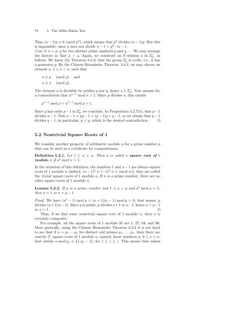
78 5. The Miller-Rabin Test Thus (n − 1)p ≡ 0(modp 2 ), which means that p 2 divides (n − 1)p. Butthis is impossible, since p does not divide n − 1=p k · m − 1. Case 2: n = p · q for two distinct prime numbers p and q. — We may arrange the factors so that p > q. Again, we construct an F-witness a in Z∗ n,as follows. We know (by Theorem 4.4.3) that the group Z∗ p is cyclic, i.e., it has a generator g. By the Chinese Remainder Theorem 3.4.1, we may choose an element a, 1≤ a
5.2 Nontrivial Square Roots of 1 79 n has extremely many prime factors, it is useless to try to find nontrivial square roots of 1 modulo n by testing randomly chosen a. Instead, we go back to the Fermat test. Let us look at an−1 mod n a little more closely. Of course, we are only interested in odd numbers n. Thenn−1 is even, and can be written as n − 1=u · 2k for some odd number u and some k ≥ 1. Thus, an−1 ≡ ((au )modn) 2k mod n, which means that we may calculate an−1 mod n with k + 1 intermediate steps: if we let b0 = a u mod n; bi =(b 2 i−1) modn, for i =1,...,k, then bk = a n−1 mod n. For example, for n = 325 = 5 2 · 13 we get n − 1= 324 = 81 · 2 2 . In Table 5.3 we calculate the powers a 81 , a 162 ,anda 324 ,all modulo 325, for several a. a b0 = a 81 b1 = a 162 b2 = a 324 2 252 129 66 7 307 324 1 32 57 324 1 49 324 1 1 65 0 0 0 126 1 1 1 201 226 51 1 224 274 1 1 Table 5.3. Powers a n−1 mod n calculated with intermediate steps, n = 325 We see that 2 is an F-witness for 325 from Z∗ 325, and 65 is an F-witness not in Z∗ 325 . In contrast, 7, 32, 49, 126, 201, and 224 are all F-liars for 325. Calculating 201 324 mod 325 with two intermediate steps leads us to detect that 51 is a nontrivial square root of 1, which proves that 325 is not prime. Similarly, the calculation with base 224 reveals that 274 is a nontrivial square root of 1. On the other hand, the corresponding calculation with bases 7, 32, or 49 does not give any information, since 7 162 ≡ 32 162 ≡−1 (mod 325) and 49 81 ≡−1 (mod 325). Similarly, calculating the powers of 126 does not reveal a nontrivial square root of 1, since 126 81 mod 325 = 1. What can the sequence b0,...,bk look like in general? We first note that if bi =1orbi = n − 1, then the remaining elements bi+1,...,bk must all equal 1, since 1 2 =1and(n − 1) 2 mod n = 1. Thus in general the sequence starts with zero or more elements /∈ {1,n− 1}, and ends with a sequence of zero or more 1’s. The two parts may or may not be separated by an entry n − 1. All possible patterns are depicted in Table 5.4, where “∗” represents an arbitrary element /∈ {1,n− 1}. We distinguish four cases:
Page 1 and 2:
Lecture Notes in Computer Science 3
Page 3 and 4:
Martin Dietzfelbinger Primality Tes
Page 5 and 6:
To Angelika, Lisa, Matthias, and Jo
Page 7 and 8:
VIII Preface toundingly it gets by
Page 9 and 10:
X Contents 5. The Miller-Rabin Test
Page 11 and 12:
2 1. Introduction: Efficient Primal
Page 13 and 14:
Page 15 and 16:
Page 17 and 18:
Page 19 and 20:
10 1. Introduction: Efficient Prima
Page 21 and 22:
12 1. Introduction: Efficient Prima
Page 23 and 24:
14 2. Algorithms for Numbers and Th
Page 25 and 26:
Page 27 and 28:
Page 29 and 30:
Page 31 and 32:
3. Fundamentals from Number Theory
Page 33 and 34: 3.1 Divisibility and Greatest Commo
Page 35 and 36: 3.2 The Euclidean Algorithm 27 Prop
Page 37 and 38: 3.2 The Euclidean Algorithm 29 (b)
Page 39 and 40: 3.2 The Euclidean Algorithm 31 We n
Page 41 and 42: 3.3 Modular Arithmetic 33 Lemma 3.3
Page 43 and 44: 3.4 The Chinese Remainder Theorem 3
Page 45 and 46: 3.4 The Chinese Remainder Theorem 3
Page 47 and 48: 3.5 Prime Numbers 39 3.5.1 Basic Ob
Page 49 and 50: 3.5 Prime Numbers 41 steps in the v
Page 51 and 52: 3.5 Prime Numbers 43 r ≥ 0. Clear
Page 53 and 54: ϕ(n) = � 3.6 Chebychev’s Theor
Page 55 and 56: 3.6 Chebychev’s Theorem on the De
Page 63 and 64: 56 4. Basics from Algebra: Groups,
Page 79 and 80: 5. The Miller-Rabin Test In this ch
Page 81 and 82: 5.1 The Fermat Test 75 multiples of
Page 83: 5.1 The Fermat Test 77 the set {n |
Page 87 and 88: 5.2 Nontrivial Square Roots of 1 81
Page 89 and 90: Lemma 5.3.1. (a) L A n ⊆ BA n . (
Page 91 and 92: 6. The Solovay-Strassen Test The pr
Page 93 and 94: 6.2 The Jacobi Symbol 87 Definition
Page 95 and 96: a 6.3 The Law of Quadratic Reciproc
Page 97 and 98: 6.3 The Law of Quadratic Reciprocit
Page 99 and 100: 6.4 Primality Testing by Quadratic
Page 101 and 102: 7. More Algebra: Polynomials and Fi
Page 103 and 104: 7.1 Polynomials over Rings 97 Defin
Page 105 and 106: 7.1 Polynomials over Rings 99 Remar
Page 107 and 108: 7.1 Polynomials over Rings 101 (b)
Page 109 and 110: 7.2 Division with Remainder and Div
Page 111 and 112: 7.3 Quotients of Rings of Polynomia
Page 113 and 114: 7.3 Quotients of Rings of Polynomia
Page 115 and 116: 7.4 Irreducible Polynomials and Fac
Page 117 and 118: 7.5 Roots of Polynomials 111 X, has
Page 119 and 120: 7.6 Roots of the Polynomial X r −
Page 121 and 122: 8. Deterministic Primality Testing
Page 123 and 124: 8.2 The Algorithm of Agrawal, Kayal
Page 125 and 126: 8.3 The Running Time 119 Time for t
Page 127 and 128: 8.3 The Running Time 121 Lemma 8.3.
Page 129 and 130: 8.5 Proof of the Main Theorem 123 B
Page 131 and 132: 8.5 Proof of the Main Theorem 125 L
Page 133 and 134: 8.5 Proof of the Main Theorem 127 P
Page 135 and 136:
8.5 Proof of the Main Theorem 129 (
Page 137 and 138:
8.5 Proof of the Main Theorem 131 i
Page 139 and 140:
134 A. Appendix Proof. For k < 0ork
Page 141 and 142:
136 A. Appendix as an abbreviation
Page 143 and 144:
138 A. Appendix a 1 2 3 4 5 6 7 8 9
Page 145 and 146:
140 A. Appendix Lemma A.3.3. If p
Page 147 and 148:
142 A. Appendix Induction step: Ass
Page 149 and 150:
144 References 20. Gauss, C.F., Dis
Page 151 and 152:
146 Index efficient algorithm, 2 eq
show all

Dietzfelbinger M. Primality testing in polynomial time ... - tiera.ru

You also want an ePaper? Increase the reach of your titles

Delete template?

Save as template?