My notes on Probability and Geometry on Groups
My notes on Probability and Geometry on Groups
My notes on Probability and Geometry on Groups

You also want an ePaper? Increase the reach of your titles
YUMPU automatically turns print PDFs into web optimized ePapers that Google loves.
<strong>Probability</strong> <strong>and</strong> <strong>Geometry</strong> <strong>on</strong> <strong>Groups</strong><br />
Lecture <str<strong>on</strong>g>notes</str<strong>on</strong>g> for a graduate course<br />
Gábor Pete<br />
Technical University of Budapest<br />
http://www.math.bme.hu/~gabor<br />
January 2, 2013<br />
Work in progress. Comments are welcome.<br />
Abstract<br />
These <str<strong>on</strong>g>notes</str<strong>on</strong>g> have grown (<strong>and</strong> are still growing) out of two graduate courses I gave at the Uni-<br />
versity of Tor<strong>on</strong>to. The main goal is to give a self-c<strong>on</strong>tained introducti<strong>on</strong> to several interrelated<br />
topics of current research interests: the c<strong>on</strong>necti<strong>on</strong>s between<br />
1) coarse geometric properties of Cayley graphs of infinite groups;<br />
2) the algebraic properties of these groups; <strong>and</strong><br />
3) the behaviour of probabilistic processes (most importantly, r<strong>and</strong>om walks, harm<strong>on</strong>ic func-<br />
ti<strong>on</strong>s, <strong>and</strong> percolati<strong>on</strong>) <strong>on</strong> these Cayley graphs.<br />
I try to be as little abstract as possible, emphasizing examples rather than presenting theorems<br />
in their most general forms. I also try to provide guidance to recent research literature. In par-<br />
ticular, there are presently over 150 exercises <strong>and</strong> many open problems that might be accessible<br />
to PhD students. It is also hoped that researchers working either in probability or in geometric<br />
group theory will find these <str<strong>on</strong>g>notes</str<strong>on</strong>g> useful to enter the other field.<br />
C<strong>on</strong>tents<br />
Preface 4<br />
1 Basic examples of r<strong>and</strong>om walks 6<br />
1.1 Z d <strong>and</strong> Td, recurrence <strong>and</strong> transience, Green’s functi<strong>on</strong> <strong>and</strong> spectral radius . . . . . 6<br />
1.2 A probability propositi<strong>on</strong>: Azuma-Hoeffding . . . . . . . . . . . . . . . . . . . . . . . 10<br />
2 Free groups <strong>and</strong> presentati<strong>on</strong>s 12<br />
2.1 Introducti<strong>on</strong> . . . . . . . . . . . . . . . . . . . . . . . . . . . . . . . . . . . . . . . . . 12<br />
2.2 Digressi<strong>on</strong> to topology: the fundamental group <strong>and</strong> covering spaces . . . . . . . . . . 13<br />
1
2.3 The main results <strong>on</strong> free groups . . . . . . . . . . . . . . . . . . . . . . . . . . . . . . 16<br />
2.4 Presentati<strong>on</strong>s <strong>and</strong> Cayley graphs . . . . . . . . . . . . . . . . . . . . . . . . . . . . . 18<br />
3 The asymptotic geometry of groups 20<br />
3.1 Quasi-isometries. Ends. The fundamental observati<strong>on</strong> of geometric group theory . . 20<br />
3.2 Gromov-hyperbolic spaces <strong>and</strong> groups . . . . . . . . . . . . . . . . . . . . . . . . . . 25<br />
3.3 Asymptotic c<strong>on</strong>es . . . . . . . . . . . . . . . . . . . . . . . . . . . . . . . . . . . . . . 25<br />
4 Nilpotent <strong>and</strong> solvable groups 25<br />
4.1 The basics . . . . . . . . . . . . . . . . . . . . . . . . . . . . . . . . . . . . . . . . . . 25<br />
4.2 Semidirect products . . . . . . . . . . . . . . . . . . . . . . . . . . . . . . . . . . . . 27<br />
4.3 The volume growth of nilpotent <strong>and</strong> solvable groups . . . . . . . . . . . . . . . . . . 31<br />
4.4 Exp<strong>and</strong>ing maps. Polynomial <strong>and</strong> intermediate volume growth . . . . . . . . . . . . 34<br />
5 Isoperimetric inequalities 37<br />
5.1 Basic definiti<strong>on</strong>s <strong>and</strong> examples . . . . . . . . . . . . . . . . . . . . . . . . . . . . . . 37<br />
5.2 Amenability, invariant means, wobbling paradoxical decompositi<strong>on</strong>s . . . . . . . . . 39<br />
5.3 From growth to isoperimetry in groups . . . . . . . . . . . . . . . . . . . . . . . . . . 42<br />
5.4 Isoperimetry in Z d . . . . . . . . . . . . . . . . . . . . . . . . . . . . . . . . . . . . . 43<br />
6 R<strong>and</strong>om walks, discrete potential theory, martingales 44<br />
6.1 Markov chains, electric networks <strong>and</strong> the discrete Laplacian . . . . . . . . . . . . . . 45<br />
6.2 Dirichlet energy <strong>and</strong> transience . . . . . . . . . . . . . . . . . . . . . . . . . . . . . . 49<br />
6.3 Martingales . . . . . . . . . . . . . . . . . . . . . . . . . . . . . . . . . . . . . . . . . 51<br />
7 Cheeger c<strong>on</strong>stant <strong>and</strong> spectral gap 56<br />
7.1 Spectral radius <strong>and</strong> the Markov operator norm . . . . . . . . . . . . . . . . . . . . . 56<br />
7.2 The infinite case: the Kesten-Cheeger-Dodziuk-Mohar theorem . . . . . . . . . . . . 58<br />
7.3 The finite case: exp<strong>and</strong>ers <strong>and</strong> mixing . . . . . . . . . . . . . . . . . . . . . . . . . . 61<br />
7.4 From infinite to finite: Kazhdan groups <strong>and</strong> exp<strong>and</strong>ers . . . . . . . . . . . . . . . . . 70<br />
8 Isoperimetric inequalities <strong>and</strong> return probabilities in general 72<br />
8.1 Poincaré <strong>and</strong> Nash inequalities . . . . . . . . . . . . . . . . . . . . . . . . . . . . . . 72<br />
8.2 Evolving sets: the results . . . . . . . . . . . . . . . . . . . . . . . . . . . . . . . . . 74<br />
8.3 Evolving sets: the proof . . . . . . . . . . . . . . . . . . . . . . . . . . . . . . . . . . 76<br />
9 Speed, entropy, Liouville property, Poiss<strong>on</strong> boundary 80<br />
9.1 Speed of r<strong>and</strong>om walks . . . . . . . . . . . . . . . . . . . . . . . . . . . . . . . . . . . 80<br />
9.2 The Liouville property for harm<strong>on</strong>ic functi<strong>on</strong>s . . . . . . . . . . . . . . . . . . . . . . 84<br />
9.3 Entropy, <strong>and</strong> the main equivalence theorem . . . . . . . . . . . . . . . . . . . . . . . 86<br />
9.4 Liouville <strong>and</strong> Poiss<strong>on</strong> . . . . . . . . . . . . . . . . . . . . . . . . . . . . . . . . . . . . 89<br />
9.5 The Poiss<strong>on</strong> boundary <strong>and</strong> entropy. The importance of group-invariance . . . . . . . 93<br />
2
9.6 Unbounded measures . . . . . . . . . . . . . . . . . . . . . . . . . . . . . . . . . . . . 96<br />
10 Growth of groups, of harm<strong>on</strong>ic functi<strong>on</strong>s <strong>and</strong> of r<strong>and</strong>om walks 98<br />
10.1 A proof of Gromov’s theorem . . . . . . . . . . . . . . . . . . . . . . . . . . . . . . . 98<br />
10.2 R<strong>and</strong>om walks <strong>on</strong> groups are at least diffusive . . . . . . . . . . . . . . . . . . . . . . 103<br />
11 Harm<strong>on</strong>ic Dirichlet functi<strong>on</strong>s <strong>and</strong> Uniform Spanning Forests 104<br />
11.1 Harm<strong>on</strong>ic Dirichlet functi<strong>on</strong>s . . . . . . . . . . . . . . . . . . . . . . . . . . . . . . . 104<br />
11.2 Loop-erased r<strong>and</strong>om walk, uniform spanning trees <strong>and</strong> forests . . . . . . . . . . . . . 105<br />
12 Percolati<strong>on</strong> theory 108<br />
12.1 Percolati<strong>on</strong> <strong>on</strong> infinite groups: pc, pu, unimodularity, <strong>and</strong> general invariant percolati<strong>on</strong>s108<br />
12.2 Percolati<strong>on</strong> <strong>on</strong> finite graphs. Threshold phenomema . . . . . . . . . . . . . . . . . . 125<br />
12.3 Critical percolati<strong>on</strong>: the plane, scaling limits, critical exp<strong>on</strong>ents, mean field theory . 129<br />
12.4 <strong>Geometry</strong> <strong>and</strong> r<strong>and</strong>om walks <strong>on</strong> percolati<strong>on</strong> clusters . . . . . . . . . . . . . . . . . . 138<br />
13 Further spatial models 143<br />
13.1 Ising, Potts, <strong>and</strong> the FK r<strong>and</strong>om cluster models . . . . . . . . . . . . . . . . . . . . . 143<br />
13.2 Bootstrap percolati<strong>on</strong> <strong>and</strong> zero temperature Glauber dynamics . . . . . . . . . . . . 153<br />
13.3 Minimal Spanning Forests . . . . . . . . . . . . . . . . . . . . . . . . . . . . . . . . . 154<br />
13.4 Measurable group theory <strong>and</strong> orbit equivalence . . . . . . . . . . . . . . . . . . . . . 157<br />
14 Local approximati<strong>on</strong>s to Cayley graphs 161<br />
14.1 Unimodularity <strong>and</strong> soficity . . . . . . . . . . . . . . . . . . . . . . . . . . . . . . . . . 161<br />
14.2 Spectral measures <strong>and</strong> other probabilistic questi<strong>on</strong>s . . . . . . . . . . . . . . . . . . . 167<br />
15 Some more exotic groups 178<br />
15.1 Self-similar groups of finite automata . . . . . . . . . . . . . . . . . . . . . . . . . . . 178<br />
15.2 C<strong>on</strong>structing m<strong>on</strong>sters using hyperbolicity . . . . . . . . . . . . . . . . . . . . . . . . 184<br />
15.3 Thomps<strong>on</strong>’s group F . . . . . . . . . . . . . . . . . . . . . . . . . . . . . . . . . . . . 184<br />
16 Quasi-isometric rigidity <strong>and</strong> embeddings 184<br />
References 186<br />
3
Preface<br />
These <str<strong>on</strong>g>notes</str<strong>on</strong>g> have grown (<strong>and</strong> are still growing) out of two graduate courses I gave at the University<br />
of Tor<strong>on</strong>to: <strong>Probability</strong> <strong>and</strong> <strong>Geometry</strong> <strong>on</strong> <strong>Groups</strong> in the Fall of 2009, <strong>and</strong> Percolati<strong>on</strong> in the plane,<br />
<strong>on</strong> Z d , <strong>and</strong> bey<strong>on</strong>d in the Spring of 2011. I am still adding material <strong>and</strong> polishing the existing parts,<br />
so at the end I expect it to be enough for two semesters, or even more. Large porti<strong>on</strong>s of the first<br />
drafts were written up by the nine students who took the first course for credit: Eric Hart, Siyu Liu,<br />
Kostya Matveev, Jim McGarva, Ben Rifkind, Andrew Stewart, Kyle Thomps<strong>on</strong>, Lluís Vena, <strong>and</strong><br />
Jeremy Voltz — I am very grateful to them. That first course was completely introductory: some<br />
students had not really seen probability before this, <strong>and</strong> <strong>on</strong>ly few had seen geometric group theory.<br />
Here is the course descripti<strong>on</strong>:<br />
<strong>Probability</strong> is <strong>on</strong>e of the fastest developing areas of mathematics today, finding new c<strong>on</strong>necti<strong>on</strong>s to<br />
other branches c<strong>on</strong>stantly. One example is the rich interplay between large-scale geometric properties<br />
of a space <strong>and</strong> the behaviour of stochastic processes (like r<strong>and</strong>om walks <strong>and</strong> percolati<strong>on</strong>) <strong>on</strong> the space.<br />
The obvious best source of discrete metric spaces are the Cayley graphs of finitely generated groups,<br />
especially that their large-scale geometric (<strong>and</strong> hence, probabilistic) properties reflect the algebraic<br />
properties. A famous example is the c<strong>on</strong>structi<strong>on</strong> of exp<strong>and</strong>er graphs using group representati<strong>on</strong>s,<br />
another <strong>on</strong>e is Gromov’s theorem <strong>on</strong> the equivalence between a group being almost nilpotent <strong>and</strong> the<br />
polynomial volume growth of its Cayley graphs. The course will c<strong>on</strong>tain a large variety of interrelated<br />
topics in this area, with an emphasis <strong>on</strong> open problems.<br />
What I had originally planned to cover turned out to be ridiculously much, so a lot had to<br />
be dropped, which is also visible in the present state of these <str<strong>on</strong>g>notes</str<strong>on</strong>g>. The main topics that are<br />
still missing are Gromov-hyperbolic groups <strong>and</strong> their applicati<strong>on</strong>s to the c<strong>on</strong>structi<strong>on</strong> of interesting<br />
groups, metric embeddings of groups in Hilbert spaces, more <strong>on</strong> the c<strong>on</strong>structi<strong>on</strong> <strong>and</strong> applicati<strong>on</strong>s of<br />
exp<strong>and</strong>er graphs, more <strong>on</strong> critical spatial processes in the plane <strong>and</strong> their scaling limits, <strong>and</strong> a more<br />
thorough study of Uniform Spanning Forests <strong>and</strong> ℓ 2 -Betti numbers — I am planning to improve the<br />
<str<strong>on</strong>g>notes</str<strong>on</strong>g> regarding these issues so<strong>on</strong>. Besides research papers I like, my primary sources were [DrK09],<br />
[dlHar00] for geometric group theory <strong>and</strong> [LyPer10], [Per04], [Woe00] for probability. I did not use<br />
more of [HooLW06], [Lub94], [Wil09] <strong>on</strong>ly because of the time c<strong>on</strong>straints. There are proofs or even<br />
secti<strong>on</strong>s that follow rather closely <strong>on</strong>e of these books, but there are always differences in the details,<br />
<strong>and</strong> the devil might be in those. Also, since I was a graduate student of Yuval Peres not too l<strong>on</strong>g<br />
ago, several parts of these <str<strong>on</strong>g>notes</str<strong>on</strong>g> are str<strong>on</strong>gly influenced by his lectures. In particular, Chapter 9<br />
c<strong>on</strong>tains paragraphs that are almost just copied from some unpublished <str<strong>on</strong>g>notes</str<strong>on</strong>g> of his that I was <strong>on</strong>ce<br />
editing. There is <strong>on</strong>e more recent book, [Gri10], whose first few chapters have c<strong>on</strong>siderable overlap<br />
with the more introductory parts of these <str<strong>on</strong>g>notes</str<strong>on</strong>g>, although I did not look at that book before having<br />
finished most of these <str<strong>on</strong>g>notes</str<strong>on</strong>g>. Anyway, the group theoretical point of view is missing from that book<br />
entirely.<br />
With all these books available, what is the point in writing these <str<strong>on</strong>g>notes</str<strong>on</strong>g>? An obvious reas<strong>on</strong> is<br />
that it is rather uncomfortable for the students to go to several different books <strong>and</strong> start reading<br />
them somewhere from their middle. Moreover, these books are usually for a bit more specialized<br />
4
audience, so either nilpotent groups or martingales are not explained carefully. So, I wanted to add<br />
my favourite explanati<strong>on</strong>s <strong>and</strong> examples to everything, <strong>and</strong> include proofs I have not seen elsewhere<br />
in the literature. And there was a very important goal I had: presenting the material in c<strong>on</strong>stant<br />
c<strong>on</strong>versati<strong>on</strong> between the probabilistic <strong>and</strong> geometric group theoretical ideas. I hope this will help<br />
not <strong>on</strong>ly students, but also researchers from either field get interested <strong>and</strong> enter the other territory.<br />
There are presently over 150 exercises, in several categories of difficulty: the <strong>on</strong>es without any<br />
stars should be doable by every<strong>on</strong>e who follows the <str<strong>on</strong>g>notes</str<strong>on</strong>g>, though they are often not quite trivial; *<br />
means it is a challenge for the reader; ** means that I think I would be able to do it, but it would be a<br />
challenge for me; *** means it is an open problem. Part of the grading scheme was to submit exercise<br />
soluti<strong>on</strong>s worth 8 points, where each exercise was worth 2 # of stars . There are also c<strong>on</strong>jectures <strong>and</strong><br />
questi<strong>on</strong>s in the <str<strong>on</strong>g>notes</str<strong>on</strong>g> — the difference compared to the *** exercises is that, according to my<br />
knowledge or feeling, the *** exercises have not been worked <strong>on</strong> yet thoroughly enough, so I want<br />
to encourage the reader to try <strong>and</strong> attack them. Of course, this does not necessarily mean that all<br />
c<strong>on</strong>jectures are hard, neither that any of the *** exercises are doable.... But, e.g., for a PhD topic,<br />
I would pers<strong>on</strong>ally suggest starting with the *** exercises.<br />
Besides my students <strong>and</strong> the books menti<strong>on</strong>ed above, I am grateful to Alex Bloemendal, Damien<br />
Gaboriau, Gady Kozma, Russ Ly<strong>on</strong>s, Péter Mester, Yuval Peres, Mark Sapir, Andreas Thom, Ádám<br />
Timár, Todor Tsankov <strong>and</strong> Bálint Virág for c<strong>on</strong>versati<strong>on</strong>s <strong>and</strong> comments.<br />
5
1 Basic examples of r<strong>and</strong>om walks<br />
1.1 Z d <strong>and</strong> Td, recurrence <strong>and</strong> transience, Green’s functi<strong>on</strong> <strong>and</strong> spectral<br />
radius<br />
In simple r<strong>and</strong>om walk <strong>on</strong> a c<strong>on</strong>nected, bounded degree infinite graph G = (V, E), we take a<br />
starting vertex, <strong>and</strong> then each step in the walk is taken to <strong>on</strong>e of the vertices directly adjacent to<br />
the <strong>on</strong>e currently occupied, uniformly at r<strong>and</strong>om, independently from all previous steps. Denote the<br />
positi<strong>on</strong>s in this walk by the sequence X0, X1, . . ., each Xi ∈ V (G).<br />
Definiti<strong>on</strong> 1.1. A r<strong>and</strong>om walk <strong>on</strong> a graph is called recurrent if the starting vertex is visited<br />
infinitely often with probability <strong>on</strong>e. That is:<br />
�<br />
Po Xn = o infinitely often � = P � Xn = o infinitely often � � X0 = o � = 1 .<br />
Otherwise, the walk is called transient.<br />
The result that started the area of r<strong>and</strong>om walks <strong>on</strong> groups is the following:<br />
Theorem 1.1 (Pólya 1920). Simple r<strong>and</strong>om walk <strong>on</strong> Z d is recurrent for d = 1, 2 <strong>and</strong> transient for<br />
d ≥ 3. In fact, the so-called “<strong>on</strong>-diag<strong>on</strong>al heat-kernel decay” is pn(o, o) = Po[ Xn = o] ≍ Cdn −d/2 .<br />
For the proof, we will need the following two lemmas. The proof of the first <strong>on</strong>e is trivial from<br />
Stirling’s formula, the proof of the sec<strong>on</strong>d <strong>on</strong>e will be discussed later.<br />
Lemma 1.2. Given a 1-dimensi<strong>on</strong>al simple r<strong>and</strong>om walk Y0, Y1, . . ., then<br />
P[ Yn = 0 ] = 1<br />
2n � �<br />
n<br />
≍<br />
n/2<br />
1<br />
√ .<br />
n<br />
Lemma 1.3. The following estimate holds for a d-dimensi<strong>on</strong>al lattice:<br />
�<br />
P # of steps am<strong>on</strong>g first n that are in the i th coordinate /∈<br />
�<br />
n 3n<br />
,<br />
2d 2d<br />
� �<br />
< C exp(−cdn).<br />
Proof of Theorem 1.1. Let o = 0 ∈ Zd denote the origin, Xn = (X1 n , . . .,Xd n ) the walk, <strong>and</strong> n =<br />
(n1, . . . , nd) a multi-index, with |n| := n1 + · · · + nd. Furthermore, let Si = Si (X1, . . . , Xn) denote<br />
the number of steps taken in the ith coordinate, i = 1, . . .,d. Then<br />
Po[ Xn = o] = Po[ X i � � i<br />
n = 0 ∀i ] = Po Y = 0 ∀i ni � � i<br />
S = ni ∀i � P[ S i = ni ∀i ] ,<br />
|n|=n<br />
which we got by using the Law of Total <strong>Probability</strong> <strong>and</strong> Bayes’ Theorem, <strong>and</strong> where the sequences<br />
Y i ni are the comp<strong>on</strong>ents of the sequence X0, X1, . . . with the null moves deleted. That is, if in the<br />
r<strong>and</strong>om walk we move from <strong>on</strong>e node to <strong>on</strong>e of the two adjacent nodes in the i th coordinate, then<br />
Y i ni changes by <strong>on</strong>e corresp<strong>on</strong>dingly, <strong>and</strong> ni increases by <strong>on</strong>e.<br />
6<br />
{s.1}<br />
{ss.ZdTd}<br />
{t.Polya}<br />
{l.Stirling}<br />
{l.LD}
Using the independence of the steps taken <strong>and</strong> Lemma 1.2, the last formula becomes<br />
Po[ Xn = o] ≍ �<br />
(n1 · · ·nd) −1/2 P[ S i = ni ∀i ]<br />
≍<br />
|n|=n<br />
�<br />
∃ni /∈[ n 3n<br />
2d , 2d ]<br />
ǫ(n) · P[ S i = ni ∀i ] + �<br />
∀ni∈[ n 3n<br />
2d , 2d ]<br />
where ǫ(n) ∈ [0, 1]. Now, by Lemma 1.3,<br />
�<br />
P[ S i = ni ∀i ] ≤ C · d · exp(−cdn),<br />
∃ni /∈[ n 3n<br />
2d , 2d ]<br />
Cd · n −d/2 · P[ S i = ni ∀i ],<br />
hence the first term in (1.1) is exp<strong>on</strong>entially small, while the sec<strong>on</strong>d term is polynomially large, so<br />
we get<br />
as claimed.<br />
Now notice that<br />
(1.1) {e.twosums}<br />
Po[ Xn = o] ≍ Cdn −d/2 , (1.2) {e.Zdret}<br />
� �<br />
Eo # of visits to o =<br />
∞�<br />
pn(o, o).<br />
� � � �<br />
Thus, from (1.2) we get for d ≥ 3 that Eo # of visits to o < ∞, hence Po # visits to o is ∞ = 0,<br />
so the r<strong>and</strong>om walk is transient.<br />
� �<br />
Also, for d = 1, 2 we get that Eo # of visits to o = ∞. However, this is not yet quite enough<br />
to claim that the r<strong>and</strong>om walk is recurrent. Here is a way to finish the proof — it may be somewhat<br />
n=0<br />
too fancy, but the techniques introduced will also be used later.<br />
Definiti<strong>on</strong> 1.2. For simple r<strong>and</strong>om walk <strong>on</strong> a graph G = (V, E), let Green’s functi<strong>on</strong> be defined<br />
as<br />
In particular,<br />
Let us also define<br />
G(x, y|z) =<br />
∞�<br />
pn(x, y)z n , x, y ∈ V (G) <strong>and</strong> z ∈ C .<br />
n=0<br />
� �<br />
G(x, y|1) = Ex # of visits to y .<br />
U(x, y|z) =<br />
∞�<br />
Px[τ y = n]z n ,<br />
n=1<br />
where τ y is the first positive time hitting y, so that Px[τ x = 0] = 0.<br />
Now, we have pn(x, x) = �n k=1 Px[τ x = k] pn−k(x, x), from which we get<br />
pn(x, x)z n n�<br />
= Px[τ x = k] z k pn−k(x, x)z n−k ,<br />
k=1<br />
∞�<br />
pn(x, x)z n = U(x, x|z)G(x, x|z),<br />
n=1<br />
G(x, x|z) − 1 = U(x, x|z)G(x, x|z),<br />
G(x, x|z) =<br />
{d.GU}<br />
1<br />
. (1.3) {e.GU}<br />
1 − U(x, x|z)<br />
7
As we proved above, for d = 1, 2 we have Ex[ # of visits to x] = ∞, hence G(x, x|1) = ∞.<br />
Thus (1.3) says that U(x, x|1) = 1, which means that Px[τ x < ∞] = 1, which clearly implies<br />
recurrence: if we come back <strong>on</strong>ce almost surely, then we will come back again <strong>and</strong> again. (To be<br />
rigorous, we need the so-called Str<strong>on</strong>g Markov property for simple r<strong>and</strong>om walk, which is intuitively<br />
obvious.)<br />
Instead of using Green’s functi<strong>on</strong>, here is a simpler proof of recurrence (though the real math<br />
c<strong>on</strong>tent is probably the same). Assume Px[τ x < ∞] = q < 1. Then<br />
a geometric r<strong>and</strong>om variable. Therefore,<br />
P[ # of returns = k ] = q k (1 − q) for k = 0, 1, 2, . . .,<br />
E[ # of returns] = q/(1 − q) < ∞ .<br />
Thus, the infinite expectati<strong>on</strong> we had for d = 1, 2 implies recurrence.<br />
Once we have encoded our sequence pn(x, y) into a power series, it is probably worth looking<br />
at the radius of c<strong>on</strong>vergence of this G(x, y|z), denoted by rad(x, y). By the Cauchy-Hadamard<br />
criteri<strong>on</strong>,<br />
A useful classical theorem is the following:<br />
1<br />
rad(x, y) =<br />
n limsupn→∞ � ≥ 1 .<br />
pn(x, x)<br />
Theorem 1.4 (Pringsheim’s theorem). If f(z) = �<br />
n anz n with an ≥ 0, then the radius rad(f) of<br />
c<strong>on</strong>vergence is the smallest positive singularity of f(z).<br />
⊲ Exercise 1.1. Prove that for simple r<strong>and</strong>om walk <strong>on</strong> a c<strong>on</strong>nected graph, for real z > 0,<br />
G(x, y|z) < ∞ ⇔ G(r, w|z) < ∞ .<br />
Therefore, by Theorem 1.4, we have that rad(x, y) is independent of x, y.<br />
By this exercise, we can define<br />
ρ :=<br />
{t.Pringsheim}<br />
1 �<br />
n<br />
= limsup pn(x, x) ≤ 1 , (1.4) {e.rho}<br />
rad(x, y) n→∞<br />
which is independent of x, y, <strong>and</strong> is called the spectral radius of the simple r<strong>and</strong>om walk <strong>on</strong> the<br />
graph. We will see later in the course the reas<strong>on</strong> for this name.<br />
Now, an obvious fundamental questi<strong>on</strong> is when ρ is smaller than 1. I.e., <strong>on</strong> what graphs are the<br />
return probabilities exp<strong>on</strong>entially small? We have seen that they are polynomial <strong>on</strong> Z d . The walk<br />
has a very different behaviour <strong>on</strong> regular trees. The simplest difference is the rate of escape:<br />
In Z, or any Z d , E[ dist(Xn, X0)] ≍ √ n, a homework from the Central Limit Theorem.<br />
8
For the k-regular tree Tk, k ≥ 3, let dist(Xn, X0) = Dn. Then<br />
On the other h<strong>and</strong>, E � Dn+1 − Dn<br />
P � Dn+1 = Dn + 1|Dn �= 0 � k − 1<br />
=<br />
k<br />
<strong>and</strong> P � Dn+1 = Dn − 1|Dn �= 0 � = 1<br />
k ,<br />
hence E � Dn+1 − Dn|Dn �= 0 � =<br />
�<br />
� Dn = 0 � = 1. Altogether,<br />
E � Dn<br />
� k − 2<br />
≥ n .<br />
k<br />
k − 1<br />
k<br />
− 1<br />
k .<br />
So, the r<strong>and</strong>om walk escapes much faster <strong>on</strong> Tk than <strong>on</strong> any Z d . This big difference will also be<br />
visible in the return probabilities.<br />
Theorem 1.5. The spectral radius of the k-regular tree Tk is ρ(Tk) = 2√ k−1<br />
k .<br />
We first give a proof using generating functi<strong>on</strong>s, then a completely probabilistic proof.<br />
Proof. With the generating functi<strong>on</strong> of Definiti<strong>on</strong> 1.2, c<strong>on</strong>sider U(z) = U(x, y|z), where x is a<br />
neighbour of y (which we will often write as x ∼ y). By taking a step <strong>on</strong> Tk, we see that either<br />
we hit y, with probability 1<br />
k−1<br />
k , or we move to another neighbour of x, with probability k , in which<br />
case, in order to hit y, we have to first return to x <strong>and</strong> then hit y. So, by the symmetries of Tk,<br />
which gives<br />
Note that if 0 ≤ z ≤ 1, then<br />
U(z) = 1 k − 1<br />
z +<br />
k k zU(z)2 ,<br />
U(z) = k ± � k 2 − 4(k − 1)z 2<br />
2(k − 1)z<br />
U(z) = Px[ ever reaching y if we die at each step with probability 1 − z ] .<br />
So, in particular, U(0) is 0, <strong>and</strong> we get U(z) = k−√k2−4(k−1)z2 2(k−1)z . Then,<br />
<strong>and</strong> thus<br />
U(x, x|z) = zU(x, y|z) = k − � k 2 − 4(k − 1)z 2<br />
2(k − 1)<br />
1<br />
G(x, x|z) =<br />
1 − U(x, y|z)<br />
2(k − 1)<br />
=<br />
k − 2 + � k2 .<br />
− 4(k − 1)z2 The smallest positive singularity is z = k<br />
2 √ k−1 , so Pringheim’s Theorem 1.4 gives ρ(Tk) = 2√ k−1<br />
k .<br />
⊲ Exercise 1.2. Compute ρ(Tk,ℓ), where Tk,ℓ is a tree such that if vn ∈ Tk,ℓ is a vertex at distance n<br />
from the root,<br />
deg vn =<br />
� k n even<br />
9<br />
ℓ n odd<br />
.<br />
,<br />
{t.treerho}<br />
(1.5) {e.GreenTree}
The next three exercises provide a probabilistic proof of Theorem 1.5, in a more precise form.<br />
(But note that the correcti<strong>on</strong> factor n −3/2 of Exercise 1.5 can also be obtained by analyzing the<br />
singularities of the generating functi<strong>on</strong>s.) This probabilistic strategy might be known to a lot of<br />
people, but I do not know any reference.<br />
⊲ Exercise 1.3. Show that for biased SRW <strong>on</strong> Z, i.e., P[ Xn+1 = j + 1 | Xn = j ] = p,<br />
�<br />
P0 Xi > 0 for 0 < i < n � � Xn = 0 � ≍ 1<br />
n ,<br />
with c<strong>on</strong>stants independent of p ∈ (0, 1). (Hint: first show, using the reflecti<strong>on</strong> principle [Dur96, Sec-<br />
ti<strong>on</strong> 3.3], that for symmetric simple r<strong>and</strong>om walk, P0[ Xi > 0 for all 0 < i ≤ 2n ] = P0[ X2n = 0 ].)<br />
⊲ Exercise 1.4. * For biased SRW <strong>on</strong> Z, show that there is a subexp<strong>on</strong>entially growing functi<strong>on</strong><br />
g(m) = exp(o(m)) such that<br />
�<br />
P0 #{i : Xi = 0 for 0 < i < n} = m � � Xn = 0 � ≤ g(m) 1<br />
n .<br />
(Hint: count all possible m-element zero sets, together with a good bound <strong>on</strong> the occurrence of each.)<br />
⊲ Exercise 1.5. Note that for SRW <strong>on</strong> the k-regular tree Tk, the distance process Dn = dist(X0, Xn)<br />
is a biased SRW <strong>on</strong> Z reflected at 0.<br />
a) Using this <strong>and</strong> Exercise 1.3, prove that the return probabilities <strong>on</strong> Tk satisfy<br />
c1 n −3/2 ρ n ≤ pn(x, x) ≤ c2 n −1/2 ρ n ,<br />
for some c<strong>on</strong>stants ci depending <strong>on</strong>ly <strong>on</strong> k, where ρ = ρ(Tk) is given by Theorem 1.5.<br />
(b) Using Exercise 1.4, improve this to<br />
with c<strong>on</strong>stants depending <strong>on</strong>ly <strong>on</strong> k.<br />
pn(x, x) ≍ n −3/2 ρ n ,<br />
1.2 A probability propositi<strong>on</strong>: Azuma-Hoeffding<br />
We discuss now a result needed for the r<strong>and</strong>om walk estimates in the previous secti<strong>on</strong>.<br />
Propositi<strong>on</strong> 1.6 (Azuma-Hoeffding). Let X1, X2, . . . be r<strong>and</strong>om variables satisfying the following<br />
criteria:<br />
• E � �<br />
Xi = 0 ∀i.<br />
• More generally, E � Xi1 · · · Xik<br />
• �Xi� ∞ < ∞ ∀i.<br />
Then, for any L > 0,<br />
� = 0 for any k ∈ Z+ <strong>and</strong> i1 < i2 < · · · < ik.<br />
P � X1 + · · · + Xn > L � ≤ e −L2 /(2 P n<br />
i=1 �Xi�2<br />
∞ ) .<br />
10<br />
{ex.nozeros}<br />
{ex.zeros}<br />
{ex.tree3/2}<br />
{ss.LD}<br />
{p.Azuma}
Proof. Define Sn := X1 + · · · + Xn. Choose any t > 0. We have<br />
P � Sn > L � ≤ P � e tSn � tL<br />
> e<br />
≤ e −tL E � � tSn<br />
e (by Markov’s inequality).<br />
By the c<strong>on</strong>vexity of e x , for |x| ≤ a, we have<br />
If we set ai := �Xi� ∞ , we get<br />
Since<br />
we see that<br />
e tx ≤ cosh(at) + xsinh(at).<br />
E � e tXi � ≤ E � cosh(ait) � + E � Xi sinh(ait) � = cosh(ait).<br />
cosh(ait) =<br />
∞�<br />
k=1<br />
(ait) 2k<br />
(2k)! ≤<br />
∞�<br />
k=1<br />
(ait) 2k<br />
2 k k!<br />
P � Sn > L � ≤ e −tL e P n<br />
i=1 �Xi�2<br />
∞ t2 /2 .<br />
= ea2<br />
i t2 /2<br />
,<br />
We optimize the bound by setting t = L/ �n 2<br />
i=1 �Xi�∞ , proving the propositi<strong>on</strong>.<br />
For an i.i.d. sequence, with E � �<br />
Xi = µ <strong>and</strong> �Xi�∞ = γ, for any α > µ we get<br />
P � Sn > αn � � � � �<br />
2<br />
α − µ<br />
≤ exp − n ,<br />
2γ<br />
which immediately implies Lemma 1.3, where we have γ = 1 <strong>and</strong> µ = 1/d.<br />
For an i.i.d. Bernoulli sequence, Xi ∼ Ber(p), this exp<strong>on</strong>ential bound is am<strong>on</strong>g the most basic<br />
tools in discrete probability, usually called Chernoff’s inequality, see, e.g., [AloS00, Appendix]. In<br />
fact, for general i.i.d., not even necessarily bounded, sequences, for any α > µ = E � �<br />
Xi , the limit<br />
logP<br />
lim<br />
n→∞<br />
� Sn > αn �<br />
= −γ(α)<br />
n<br />
always exists. The functi<strong>on</strong> γ(α) is called the large deviati<strong>on</strong> rate functi<strong>on</strong> (associated with the<br />
distributi<strong>on</strong> of Xi). Moreover, in order to ensure γ(α) > 0, instead of boundedness, it is enough<br />
that the moment generating functi<strong>on</strong> E � e tX � is finite for some t > 0. The rate functi<strong>on</strong> can be<br />
computed in terms of the moment generating functi<strong>on</strong>, <strong>and</strong>, e.g., for Xi ∼ Ber(p) it is<br />
γp(α) = α log α 1 − α<br />
+ (1 − α)log . (1.6) {e.LDBinomial}<br />
p 1 − p<br />
See, e.g., [Dur96, Secti<strong>on</strong> 1.9] <strong>and</strong> [Bil86, Secti<strong>on</strong> 1.9] for these results.<br />
The main point of Propositi<strong>on</strong> 1.6 is its generality: the uncorrelatedness c<strong>on</strong>diti<strong>on</strong>s for the Xi’s,<br />
besides i.i.d. sequences, are also fulfilled by martingale differences Xi = Mi+1 − Mi, where {Mi} ∞ i=0<br />
is a martingale sequence. See Secti<strong>on</strong> 6.3 for the definiti<strong>on</strong> <strong>and</strong> examples.<br />
11
2 Free groups <strong>and</strong> presentati<strong>on</strong>s<br />
2.1 Introducti<strong>on</strong><br />
Definiti<strong>on</strong> 2.1 (Fk, the free group <strong>on</strong> k generators). Let a1, a2, . . . , ak, a −1<br />
1<br />
, a−1 2<br />
, . . .,a−1 k be symbols.<br />
The elements of the free group generated by {a1, . . . , ak} are the finite reduced words: remove any<br />
aia −1<br />
i or a −1<br />
i ai, <strong>and</strong> group multiplicati<strong>on</strong> is c<strong>on</strong>catenati<strong>on</strong> (then reducti<strong>on</strong> if needed).<br />
Lemma 2.1. Every word has a unique reduced word. (Proof by inducti<strong>on</strong>.)<br />
Propositi<strong>on</strong> 2.2. If S is a set <strong>and</strong> FS is the free group generated by S, <strong>and</strong> Γ is any group, then<br />
for any map f : S −→ Γ there is a group homomorphism ˆ f : FS −→ Γ extending f.<br />
Proof. Define ˆ f(s i1<br />
1<br />
· · ·sik<br />
k ) = f(s1) i1 · · · f(sk) ik , then check that this is a homomorphism.<br />
Corollary 2.3. Every group is a quotient of a free group.<br />
Proof. Lazy soluti<strong>on</strong>: take S = Γ, then there is an <strong>on</strong>to map FS −→ Γ. A less lazy soluti<strong>on</strong> is to<br />
take a generating set, Γ = 〈S〉. Then, by the propositi<strong>on</strong>, there is a surjective map ˆ f : FS −→ Γ<br />
with ker( ˆ f) ⊳ FS, hence FS/ ker( ˆ f) ≃ Γ.<br />
Definiti<strong>on</strong> 2.2. Given a generating set S <strong>and</strong> a set of relati<strong>on</strong>s R of elements of S, a presentati<strong>on</strong><br />
of Γ is given by 〈S〉 mod the relati<strong>on</strong>s in R. This is written Γ = 〈S|R〉. More formally, Γ ≃ 〈S〉/〈〈R〉〉<br />
where R ⊂ FS <strong>and</strong> 〈〈R〉〉 is the smallest normal subgroup c<strong>on</strong>taining R. A group is called finitely<br />
presented if both R <strong>and</strong> S can be chosen to be finite sets.<br />
Example: C<strong>on</strong>sider the group Γ = 〈a1, . . . , ad | [ai, aj] ∀i, j〉, where [ai, aj] = aiaja −1<br />
i a−1<br />
j . We wish<br />
to show that this is isomorphic to the group Z d . It is clear that Γ is commutitive — if we have aiaj<br />
in a word, we can insert the commutator [aiaj] to reverse the order — so every word in Γ can be<br />
written in the form<br />
v = a n1<br />
1 an2 2 · · ·ank k .<br />
Define φ : G −→ Z d by φ(v) = (n1, n2, . . . , nk). It is now obvious that φ is an isomorphism.<br />
Definiti<strong>on</strong> 2.3. Let Γ be a finitely generated group, 〈S〉 = Γ. Then the right Cayley graph<br />
G(Γ, S) is the graph with vertex set V (G) = Γ <strong>and</strong> edge set E(G) = {(g, gs) : g ∈ Γ, s ∈ S}. The<br />
left Cayley graph is defined using left multiplicati<strong>on</strong>s by the generators. These graphs are often<br />
c<strong>on</strong>sidered to have directed edges, labeled with the generators, <strong>and</strong> then they are sometimes called<br />
Cayley diagrams. However, if S is symmetric (∀s ∈ S, s −1 ∈ S), then G is naturally undirected<br />
<strong>and</strong> |S|-regular (even if S has order 2 elements).<br />
Example: The Z d lattice is the Cayley graph of Z d with the 2d generators {ei, −ei} d i=1 .<br />
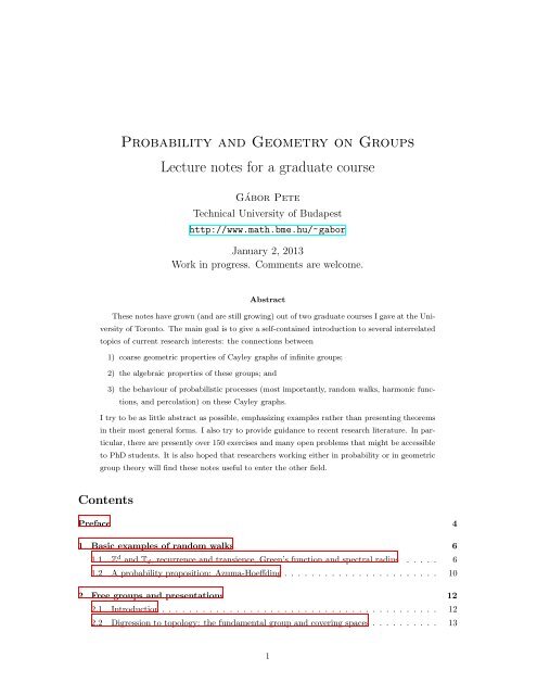
Example: The Cayley graph of F2 with generators {a, b, a −1 , b −1 } is a 4-regular tree, see Figure 2.1.<br />
Let Γ be a group with right Cayley graph G = G(Γ, S). Then Γ acts <strong>on</strong> G from the left as follows:<br />
for h ∈ Γ, an element g ∈ V (G) maps to hg, <strong>and</strong> an element (g, gs) ∈ E(G) maps to (hg, hgs). This<br />
shows that every Cayley graph is transitive.<br />
12<br />
{s.groups}<br />
{ss.groupintro}<br />
{d.Cayley}
Figure 2.1: The Cayley graph of F2. {f.F2}<br />
Finitely presentedness has important c<strong>on</strong>sequences for the geometry of the Cayley graphs, see<br />
Subsecti<strong>on</strong>s 2.4 <strong>and</strong> 3.1, <strong>and</strong> the discussi<strong>on</strong> around Propositi<strong>on</strong> 12.5. Classical examples of finitely<br />
generated n<strong>on</strong>-finitely presented groups are the lamplighter groups Z2 ≀ Z d , which will be defined<br />
in Secti<strong>on</strong> 5.1, <strong>and</strong> studied in Chapter 9 from a r<strong>and</strong>om walk point of view. The n<strong>on</strong>-finitely<br />
presentedness of Z2 ≀ Z is proved in Exercise 12.3.<br />
We have seen two effects of Tk being much more “spacious” than Z d <strong>on</strong> the behaviour of simple<br />
r<strong>and</strong>om walk: the escape speed is much larger, <strong>and</strong> the return probabilities are much smaller. It<br />
looks intuitively clear that Z <strong>and</strong> Tk should be the extremes, <strong>and</strong> that there should be a large variety<br />
of possible behaviours in between. It is indeed relatively easy to show that Tk is <strong>on</strong>e extreme am<strong>on</strong>g<br />
2k-regular Cayley-graphs, but, from the other end, it is <strong>on</strong>ly a recent theorem that the expected rate<br />
of escape is at least E � dist(X0, Xn) � ≥ c √ n <strong>on</strong> any group: see Secti<strong>on</strong> 10.2. One reas<strong>on</strong> for this not<br />
being obvious is that not every infinite group c<strong>on</strong>tains Z as a subgroup: there are finitely generated<br />
infinite groups with a finite exp<strong>on</strong>ent n: the nth power of any element is the identity. <strong>Groups</strong> with<br />
such strange properties are called Tarksi m<strong>on</strong>sters. But even <strong>on</strong> groups with a Z subgroup, there<br />
does not seem to be an easy proof.<br />
We will also see that c<strong>on</strong>structing groups with intermediate behaviours is not always easy. One<br />
reas<strong>on</strong> for this is that the <strong>on</strong>ly general way that we have seen so far to c<strong>on</strong>struct groups is via<br />
presentati<strong>on</strong>s, but there are famous undecidability results here: there is no general algorithm to<br />
decide whether a word can be reduced in a given presentati<strong>on</strong> to the empty word, <strong>and</strong> there is no<br />
general algorithm to decide if a group given by a presentati<strong>on</strong> is isomorphic to another group, even<br />
to the trivial group. So, we will need other means of c<strong>on</strong>structing groups.<br />
2.2 Digressi<strong>on</strong> to topology: the fundamental group <strong>and</strong> covering spaces<br />
Several results <strong>on</strong> free groups <strong>and</strong> presentati<strong>on</strong>s become much simpler in a topological language.<br />
The present secti<strong>on</strong> discusses the necessary background.<br />
We will need the c<strong>on</strong>cept of a CW-complex. The simplest way to define an n-dimensi<strong>on</strong>al<br />
CW-complex is to do it recursively:<br />
13<br />
{ss.topology}
• A 0-complex is a countable (finite or infinite) uni<strong>on</strong> of points, with the discrete topology.<br />
• To get an n-complex, we can glue n-cells to an n−1-complex, i.e., we add homeomorphic images<br />
of the n-balls such that each boundary is mapped c<strong>on</strong>tinuously <strong>on</strong>to a uni<strong>on</strong> of n − 1-cells.<br />
We will always assume that our topological spaces are c<strong>on</strong>nected CW-complexes.<br />
C<strong>on</strong>sider a space X <strong>and</strong> a fixed point x ∈ X. C<strong>on</strong>sider two loops α : [0, 1] −→ X <strong>and</strong> β : [0, 1] −→<br />
X starting at x. I.e., α(0) = α(1) = x = β(0) = β(1). We say that α <strong>and</strong> β are homotopic, denoted<br />
by α ∼ β, if there is a c<strong>on</strong>tinuous functi<strong>on</strong> f : [0, 1] × [0, 1] −→ X satisfying<br />
f(t, 0) = α(t), f(t, 1) = β(t), f(0, s) = f(1, s) = x ∀s ∈ [0, 1].<br />
We are ready to define the fundamental group of X. Let π1(X, x) be the set of equivalence<br />
classes of paths starting <strong>and</strong> ending at x. The group operati<strong>on</strong> <strong>on</strong> π1 is induced by c<strong>on</strong>catenati<strong>on</strong><br />
of paths:<br />
⎧<br />
⎨α(2t)<br />
t ∈ [0,<br />
αβ(t) =<br />
⎩<br />
1<br />
2 ]<br />
β(2t − 1) t ∈ [ 1<br />
.<br />
, 1]<br />
While it seems from the definiti<strong>on</strong> that the fundamental group would depend <strong>on</strong> the point x,<br />
this is not true. To find an isomorphism between π1(X, x) <strong>and</strong> π1(X, y), map any loop γ starting at<br />
x to a path from y to x c<strong>on</strong>catenated with γ <strong>and</strong> the same path from x back to y.<br />
The spaces X <strong>and</strong> Y are homotopy equivalent, denoted by X ∼ Y , if there exist c<strong>on</strong>tinuous<br />
functi<strong>on</strong>s f : X −→ Y <strong>and</strong> g : Y −→ X such that<br />
f ◦ g ∼ idY , g ◦ f ∼ idX.<br />
A basic result (with a simple proof that we omit) is the following:<br />
Theorem 2.4. If X ∼ Y then π1(X) ∼ = π1(Y ).<br />
Theorem 2.5. C<strong>on</strong>sider the CW-complex with a single point <strong>and</strong> k loops from this point. Denote<br />
this CW-complex by Rosek, a rose with k petals. Then π1(Rosek) = Fk.<br />
The proof of this theorem uses the Seifert-van Kampen Theorem 3.1. We do not discuss this<br />
here, but we believe the statement is intuitively obvious.<br />
Corollary 2.6. The fundamental group of any (c<strong>on</strong>nected) graph is free.<br />
Proof. For any finite c<strong>on</strong>nected graph with n vertices <strong>and</strong> l edges, c<strong>on</strong>sider a spanning tree T. Then<br />
T has n − 1 edges. C<strong>on</strong>tract T to a point x. There are k = l − n + 1 edges left over, <strong>and</strong> after<br />
the c<strong>on</strong>tracti<strong>on</strong> each begins <strong>and</strong> ends at x. C<strong>on</strong>tracti<strong>on</strong> of a spanning tree to a point is a homotopy<br />
equivalence, so the graph is homotopy equivalent to Rosek. Hence, the fundamental group is free by<br />
Theorems 2.4 <strong>and</strong> 2.5.<br />
⊲ Exercise 2.1. If Γ is a topological group then π1(Γ) is commutative. (Recall that a group Γ is a<br />
topological group if it is also a topological space such that the functi<strong>on</strong>s Γ × Γ −→ Γ : (x, y) ↦→ xy<br />
<strong>and</strong> Γ −→ Γ : x ↦→ x −1 are c<strong>on</strong>tinuous.)<br />
14<br />
2<br />
{t.fundhomotop}<br />
{t.fundRose}<br />
{c.fundgraph}
We now introduce another basic noti<strong>on</strong> of geometry:<br />
p<br />
′ Definiti<strong>on</strong> 2.4. We say that X ։ X is a covering map if for every x ∈ X, there is an open<br />
neighbourhood U ∋ x such that each c<strong>on</strong>nected comp<strong>on</strong>ent of p −1 (U) is homeomorphic to U by p.<br />
Propositi<strong>on</strong> 2.7. Let γ ⊂ X be any path starting at x. Then for every x ∗ ∈ p −1 (x) there is a<br />
unique γ ∗ starting at x ∗ with p(γ ∗ ) = γ.<br />
Sketch of proof. Because of the local homeomorphisms, there is always a unique way to c<strong>on</strong>tinue the<br />
lifted path.<br />
Theorem 2.8 (M<strong>on</strong>odromy Theorem). If γ <strong>and</strong> δ are homotopic with fixed endpoints x <strong>and</strong> y, then<br />
the lifts γ ∗ <strong>and</strong> δ ∗ starting from the same x ∗ have the same endpoints <strong>and</strong> γ ∗ ∼ δ ∗ .<br />
Sketch of proof. The homotopies can be lifted through the local homeomorphisms.<br />
The following results can be easily proved using Propositi<strong>on</strong> 2.7 <strong>and</strong> Theorem 2.8:<br />
Lemma 2.9. Any covering space of a graph is a graph.<br />
Lemma 2.10. Let x ∈ X <strong>and</strong> U ∋ x a neighbourhood as in Definiti<strong>on</strong> 2.4. Then the number k of<br />
c<strong>on</strong>nected comp<strong>on</strong>ents of p −1 (U) is independent of x <strong>and</strong> U, <strong>and</strong> the covering is called k-fold. (In<br />
fact, the lifts of any path γ between x, y ∈ X give a pairing between the preimages of x <strong>and</strong> y.)<br />
Let X be a topological space. We say that � X is a universal cover of X if:<br />
• � X is a cover.<br />
• � X is c<strong>on</strong>nected.<br />
• � X is simply c<strong>on</strong>nected, i.e., π1( � X) = 1.<br />
The existence of a universal cover is guaranteed by the following theorem:<br />
Theorem 2.11. Every c<strong>on</strong>nected CW complex X has a universal cover � X.<br />
Sketch of proof. Let the set of points of � X be the fixed endpoint homotopy classes of paths starting<br />
from a fixed x ∈ X. The topology <strong>on</strong> � X is defined by thinking of a class of paths [γ] to be close to<br />
[δ] if there are representatives γ, δ such that δ is just γ c<strong>on</strong>catenated with a short piece of path.<br />
⊲ Exercise 2.2. Write down the above definiti<strong>on</strong> of the topology <strong>on</strong> � X properly <strong>and</strong> the proof that,<br />
with this topology, π1( � X) = 1.<br />
The fundamental group π1(X) acts <strong>on</strong> � X with c<strong>on</strong>tinuous maps, as follows.<br />
Let γ ∈ π1(X, x) be a loop, p the surjective map defined by the covering � X, <strong>and</strong> x ∗ ∈ p −1 (x) a<br />
point above x. Using Propositi<strong>on</strong> 2.7 <strong>and</strong> Theorem 2.8, there exists a unique homeomorphic curve<br />
γ ∗ (not depending <strong>on</strong> the representative for γ) with starting point x ∗ <strong>and</strong> some ending point x ∗ ,<br />
which also bel<strong>on</strong>gs to p −1 (x). The acti<strong>on</strong> fγ <strong>on</strong> x ∗ is now defined by fγ(x ∗ ) = x ∗ . As we menti<strong>on</strong>ed<br />
15<br />
{d.covering}<br />
{p.uniquelift}<br />
{t.m<strong>on</strong>odromy}<br />
{l.graphcover}<br />
{l.k-fold}<br />
{t.univcover}
above, this acti<strong>on</strong> does not depend <strong>on</strong> the representative for γ, <strong>and</strong> it is clear that fδ ◦ fγ = fγδ for<br />
γ, δ ∈ π1(X, x), so we indeed have an acti<strong>on</strong> of π1(X, x) <strong>on</strong> the fibre p −1 (x).<br />
We need to define the acti<strong>on</strong> also <strong>on</strong> any y ∗ ∈ p −1 (y), y ∈ X. We take a path δ ∗ in � X from y ∗<br />
to x ∗ , then δ = p(δ ∗ ) is a path from y to x, <strong>and</strong> δγδ −1 is a path from y to itself. Since π1( � X) = 1,<br />
all possible choices of δ ∗ are homotopic to each other, hence all resulting δ <strong>and</strong> all δγδ −1 curves are<br />
homotopic. By Propositi<strong>on</strong> 2.7 <strong>and</strong> Theorem 2.8, there is a unique lift of δγδ −1 starting from y ∗ ,<br />
<strong>and</strong> its endpoint y ∗ ∈ p −1 (y) does not depend <strong>on</strong> the choice of δ ∗ . Hence we indeed get an acti<strong>on</strong> of<br />
π1(X, x) <strong>on</strong> the entire � X.<br />
This acti<strong>on</strong> permutes points inside each fibre, <strong>and</strong> it is easy to see that the acti<strong>on</strong> is free (i.e.,<br />
<strong>on</strong>ly the identity has fixed points). If we make the quotient space of � X by this group acti<strong>on</strong> (i.e.,<br />
each point of � X is mapped to its orbit under the group acti<strong>on</strong>), we will obtain X, <strong>and</strong> the quotient<br />
map is exactly the covering map p:<br />
�X/π1(X, x) = X . (2.1) {e.pi1factor}<br />
Example: The fundamental group of the torus T 2 is Z 2 . We have R 2 /Z 2 = T 2 , where R 2 is the<br />
usual covering made out of copies of the square [0, 1) × [0, 1).<br />
For each subgroup H ≤ π1(X), we can c<strong>on</strong>sider XH = � X/H, which is still a covering space of<br />
X: there is a natural surjective map from XH to X, by taking the π1(X)-orbit c<strong>on</strong>taining any given<br />
H-orbit. On the other h<strong>and</strong>, � X is the universal cover of XH, too, <strong>and</strong> we have π1(XH) ∼ = H.<br />
2.3 The main results <strong>on</strong> free groups<br />
A probably unsurprising result is the following:<br />
Theorem 2.12. Fk ∼ = Fl <strong>on</strong>ly if k = l .<br />
⊲ Exercise 2.3. Prove Theorem 2.12. (Hint 1: how many index 2 subgroups are there? Or, hint 2:<br />
What is Fk/[Fk, Fk]?)<br />
The next two results can be proved also with combinatorial arguments, but the topological<br />
language of the previous subsecti<strong>on</strong> makes things much more transparent.<br />
Theorem 2.13 (Nielsen-Schreier). Every subgroup of a free group is free.<br />
Theorem 2.14 (Schreier’s index formula). If Fk is free <strong>and</strong> Fl ≤ Fk such that [Fk : Fl] = r < ∞,<br />
then<br />
l − 1 = (k − 1)r.<br />
Proof of Theorem 2.13. Let the free group be Fk. By Theorem 2.5, we have Fk ∼ = π1(Rosek). Let G<br />
be the universal cover of Rosek. By Lemma 2.9, it is a graph; in fact, it is the 2k-regular tree T2k.<br />
Now take H ≤ Fk. As discussed at the end of the previous secti<strong>on</strong>, GH = G/H is a covering of<br />
Rosek <strong>and</strong> is covered by T2k. Again by Lemma 2.9, it is a graph, <strong>and</strong> π1(GH) = H. By Corollary 2.6,<br />
the fundamental group of a graph is free, hence H is free, proving Theorem 2.13.<br />
16<br />
{ss.freemain}<br />
{t.freeisom}<br />
{t.NieSch}<br />
{t.Schind}
Proof of Theorem 2.14. The Euler characteristic of a graph is the difference between the number of<br />
vertices <strong>and</strong> the number of edges:<br />
χ(G) = |V (G)| − |E(G)| .<br />
Homotopies of graphs increase or decrease the vertex <strong>and</strong> the edge sets by the same amount, hence χ<br />
is a homotopy invariant of graphs. Furthermore, if G ′ is an r-fold covering of G, then rχ(G) = χ(G ′ ).<br />
Since the graph Rosek has <strong>on</strong>e vertex <strong>and</strong> k edges, χ(Rosek) = 1 − k. As the index of H = Fl in<br />
Fk is r, we see that T2k/H is an r-fold covering of Rosek. Thus, χ(T2k/H) = rχ(Rosek) = r(1 − k).<br />
On the other h<strong>and</strong>, T2k/H is a graph with π1(T2k/H) = H = Fl. Since any graph is homotopic<br />
to a rose, <strong>and</strong>, by Theorems 2.5 <strong>and</strong> 2.12, different roses have n<strong>on</strong>-isomorphic fundamental groups,<br />
π1(Rosel) = Fl, we get that T2k/H must be homotopic to Rosel, <strong>and</strong> thus χ(T2k/H) = 1 − l.<br />
Therefore, we obtain r(1 − k) = 1 − l.<br />
Notice that, if 2 ≤ r < ∞ then r(1 − k) �= 1 − k.<br />
⊲ Exercise 2.4. Prove the Fk has Fk as a subgroup with infinite index.<br />
⊲ Exercise 2.5.* A finitely generated group acts <strong>on</strong> a tree freely if <strong>and</strong> <strong>on</strong>ly if the group if free. (The<br />
acti<strong>on</strong> is by graph automorphisms of the tree T, <strong>and</strong> a free acti<strong>on</strong> means that StabG(x) = {1} for<br />
any x ∈ V (T) ∪ E(T).)<br />
Hint: separate the cases where there is an element of order 2 in Γ, <strong>and</strong> where there are no such<br />
elements (in which case there is a fixed vertex, as it turns out).<br />
We will now show that a finitely generated free group is linear. For instance, F2 ≤ SL2(Z)<br />
(integer 2 × 2 matrices with determinant 1). Indeed:<br />
Lemma 2.15 (Ping-P<strong>on</strong>g Lemma). Let Γ be a group acting <strong>on</strong> some set X. Let Γ1, Γ2 be subgroups<br />
of Γ, with |Γ1| ≥ 3, <strong>and</strong> let Γ ∗ = 〈Γ1, Γ2〉. Assume that there exist n<strong>on</strong>-empty sets X1, X2 ⊆ X with<br />
X2 � X1 <strong>and</strong><br />
Then Γ1 ∗ Γ2 = Γ ∗ .<br />
γ(X2) ⊆ X1 ∀γ ∈ Γ1 \ {1} ,<br />
γ(X1) ⊆ X2 ∀γ ∈ Γ2 \ {1} .<br />
The product ∗ de<str<strong>on</strong>g>notes</str<strong>on</strong>g> the free product. If Γ1 = 〈S1|R1〉 <strong>and</strong> Γ2 = 〈S2|R2〉, then Γ1 ∗ Γ2 =<br />
〈S1, S2|R1, R2〉. In particular, Fk = Z ∗ Z ∗ · · · ∗ Z, k times.<br />
⊲ Exercise 2.6. Prove the Ping-P<strong>on</strong>g Lemma.<br />
with<br />
Now let<br />
Γ1 =<br />
�� � � �� � �<br />
1 2n<br />
1 0<br />
, n ∈ Z , Γ2 = , n ∈ Z ,<br />
0 1<br />
2n 1<br />
�� �<br />
x<br />
X1 = ∈ R<br />
y<br />
2 � �� �<br />
x<br />
, |x| > |y| , X2 = ∈ R<br />
y<br />
2 �<br />
, |x| < |y| .<br />
17<br />
{l.pingp<strong>on</strong>g}
Observe that the hypotheses of the Ping-P<strong>on</strong>g Lemma are fulfilled. Therefore, the matrices<br />
� �<br />
1 0<br />
<strong>and</strong> generate a free group.<br />
2 1<br />
⊲ Exercise 2.7. Show that the following properties of a group Γ are equivalent.<br />
(i) For every γ �= 1 ∈ Γ there is a homomorphism π <strong>on</strong>to a finite group F such that π(γ) �= 1.<br />
(ii) The intersecti<strong>on</strong> of all its subgroups of finite index is trivial.<br />
(iii) The intersecti<strong>on</strong> of all its normal subgroups of finite index is trivial.<br />
Such groups are called residually finite.<br />
� �<br />
1 2<br />
For instance, Z n , SLn(Z) <strong>and</strong> GLn(Z) are residually finite, because of the natural (mod p)<br />
homomorphisms <strong>on</strong>to (Z/pZ) n , SLn(Z/pZ) <strong>and</strong> GLn(Z/pZ).<br />
⊲ Exercise 2.8. Show that any subgroup of a residually finite group is also residually finite. C<strong>on</strong>clude<br />
that the free groups Fk are residually finite.<br />
⊲ Exercise 2.9.<br />
(i) Show that if Γ is residually finite <strong>and</strong> φ : Γ −→ Γ is a surjective homomorphism, then it is<br />
a bijecti<strong>on</strong>. (Hint: assume that kerφ is n<strong>on</strong>-trivial, show that the number of index k subgroups of<br />
Γ ≃ Γ/ kerφ is finite, then arrive at a c<strong>on</strong>tradicti<strong>on</strong>. Alternatively, show that any homomorphism π<br />
<strong>on</strong>to a finite group F must annihilate kerφ.)<br />
(ii) C<strong>on</strong>clude that if k distinct elements generate the free group Fk, then they generate it freely.<br />
2.4 Presentati<strong>on</strong>s <strong>and</strong> Cayley graphs<br />
Fix some subset of (oriented) loops in a directed Cayley graph G(Γ, S) of a group Γ = 〈S|R〉, which<br />
will be called the basic loops. A geometric c<strong>on</strong>jugate of a loop can be:<br />
• “rotate” the loop, i.e., choose another starting point in the same loop;<br />
• translate the loop in G by a group element.<br />
A combinati<strong>on</strong> of basic loops is a loop made of a sequence of loops (ℓi), where the i-th is a geometric<br />
c<strong>on</strong>jugate of a basic loop, <strong>and</strong> starts in a vertex c<strong>on</strong>tained in some ℓj, j ∈ [1, i − 1].<br />
To any loop ℓ = (g, gs1, gs1s2, . . .,gs1s2 · · · sk = g), with each si ∈ S, we can associate the word<br />
w(ℓ) = s1s2 · · · sk. So, translated copies of the same loop have the same word associated to them.<br />
Propositi<strong>on</strong> 2.16. Any loop in G(Γ, S) is homotopy equivalent to a combinati<strong>on</strong> of basic loops if<br />
<strong>and</strong> <strong>on</strong>ly if the words given by the basic loops generate 〈〈R〉〉 as a normal subgroup.<br />
Recall that 〈〈R〉〉 de<str<strong>on</strong>g>notes</str<strong>on</strong>g> the normal subgroup of the relati<strong>on</strong>s, <strong>and</strong> Γ = FS/〈〈R〉〉.<br />
Proof. Let the set of all loops in G be L, the set of basic loops B, <strong>and</strong> the set of loops produced<br />
from B by combining them <strong>and</strong> applying homotopies C. The statement of the propositi<strong>on</strong> is that<br />
C = L if <strong>and</strong> <strong>on</strong>ly if 〈〈w(B)〉〉 = 〈〈R〉〉.<br />
18<br />
0 1<br />
{ex.resfin}<br />
{ss.presentati<strong>on</strong>s}<br />
{p.loops}
We first show that 〈〈w(B)〉〉 = w(C). Let us start with the directi<strong>on</strong> ⊇.<br />
What happens to the associated word when we rotate a loop? From the word s1s2 · · · sk ∈ w(B),<br />
rotating by <strong>on</strong>e edge, say, we get s2 · · ·sks1. This new word is in fact a c<strong>on</strong>jugate of the old word:<br />
s −1<br />
1 (s1s2 · · · sk)s1, hence it is an element of 〈〈w(B)〉〉.<br />
Next, when we combine two loops, (g, gs1, . . . , gs1 · · · sn = g) <strong>and</strong> (h, ht1, . . .,ht1 · · · tm = h) into<br />
(g, . . .,gS1, gS1t1, . . .,gS1T, gS1Tsk+1, gS1TS2 = g),<br />
where S1 = s1 · · · sk, S2 = sk+1 · · ·sn <strong>and</strong> T = t1 · · · tm, then the new associated word S1TS2 equals<br />
SS −1<br />
2 TS2. Thus, combining loops does not take us out from 〈〈w(B)〉〉. See Figure 2.2 (a).<br />
Finally, if two loops are homotopic to each other in G, then we can get <strong>on</strong>e from the other by<br />
combining in a sequence of c<strong>on</strong>tractible loops, which are just “c<strong>on</strong>tour paths” of subtrees in G, i.e.,<br />
themselves are combinati<strong>on</strong>s of trivial sis −1<br />
i loops for some generators si ∈ S. See Figure 2.2 (b).<br />
The effect of these geometric combinati<strong>on</strong>s <strong>on</strong> the corresp<strong>on</strong>ding word is just plugging in trivially<br />
reducible words, wich again does not take us out from 〈〈w(B)〉〉.<br />
Figure 2.2: (a) Combining two loops. (b) Homotopic loops inside Z 2 . {f.loops}<br />
So, we have proved 〈〈w(B)〉〉 ⊇ w(C). But ⊆ is now also clear: we have encountered the geometric<br />
counterpart of all the operati<strong>on</strong>s <strong>on</strong> the words in w(B) that together produce 〈〈w(B)〉〉.<br />
On the other h<strong>and</strong>, we obviously have w(L) = 〈〈R〉〉, since a word <strong>on</strong> S is a loop in G iff the<br />
word represents 1 in Γ iff the word is in the kernel 〈〈R〉〉 of the factorizati<strong>on</strong> from the free group FS.<br />
So, the last step we need is that L = C if <strong>and</strong> <strong>on</strong>ly if w(L) = w(C). Since both L <strong>and</strong> C are<br />
closed under translati<strong>on</strong>s, this is clear.<br />
We now state an elegant topological definiti<strong>on</strong> of the Cayley graph G(Γ, S):<br />
Definiti<strong>on</strong> 2.5. Take the 1-dimensi<strong>on</strong>al CW-complex Rose |S|, <strong>and</strong> for any word in R, glue a 2-cell<br />
<strong>on</strong> it with boundary given by the word. Let X(S, R) denote the resulting 2-dimensi<strong>on</strong>al CW complex.<br />
Now take the universal cover � X(S, R). This is called the Cayley complex corresp<strong>on</strong>ding to S <strong>and</strong><br />
R. The 1-skelet<strong>on</strong> of � X(S, R) is the 2|S|-regular Cayley graph G(Γ, S) of Γ = 〈S|R〉.<br />
For instance, when S = {a, b} <strong>and</strong> R = {aba −1 b −1 }, we glue a single 2-cell, resulting in a torus,<br />
whose universal cover will be homeomorphic to R 2 , with a Z 2 lattice as its 1-skelet<strong>on</strong>.<br />
The proof that this definiti<strong>on</strong> of the Cayley graph coincides with the usual <strong>on</strong>e has roughly<br />
the same math c<strong>on</strong>tent as our previous propositi<strong>on</strong>. But here is a sketch of the story told in the<br />
19<br />
{d.CayleyCW}
language of covering surfaces: It is intuitively clear, <strong>and</strong> can be proved using the Seifert – van<br />
Kampen theorem, that π1(X(S, R)) = 〈S|R〉. Then, as we observed in (2.1), � X(S, R)/Γ = X(S, R).<br />
We can now c<strong>on</strong>sider the right Schreier graph G(Γ, � X, S) of the acti<strong>on</strong> of Γ <strong>on</strong> � X = � X(S, R) with<br />
generating set S: the vertices are the vertices of the CW complex � X (this is just <strong>on</strong>e Γ-orbit), <strong>and</strong><br />
the edges are (x ∗ , x ∗ s), where x ∗ runs through the vertices <strong>and</strong> s runs through S. Clearly, this is<br />
exactly the 1-skelet<strong>on</strong> of � X. On the other h<strong>and</strong>, since the acti<strong>on</strong> is free, this Schreier graph is just<br />
the Cayley graph G(Γ, S), <strong>and</strong> we are d<strong>on</strong>e.<br />
So, if we factorize Fk by normal subgroups, we get all possible groups Γ, <strong>and</strong> the Schreier graph<br />
of the acti<strong>on</strong> by Γ <strong>on</strong> the Cayley complex will be a 2k-regular Cayley graph. Besides the Schreier<br />
graph of a group acti<strong>on</strong>, there is another usual meaning of a Schreier graph, which is just a special<br />
case: if H ≤ Γ, <strong>and</strong> S is a generating set of Γ, then the set H\Γ of right cosets {Hg} supports a<br />
natural graph structure, Hg ∼ Hgs for s ∈ S. This graph is denoted by G(Γ, H, S).<br />
⊲ Exercise 2.10.* Show that any 2k-regular graph is the Schreier graph of Fk with respect to some<br />
subgroup H. On the other h<strong>and</strong>, the 3-regular Petersen graph is not a Schreier graph.<br />
The above results show that being finitely presented is a property with a str<strong>on</strong>g topological<br />
flavour. Indeed, it is clearly equivalent to the existence of some r < ∞ such that the Ripsr(G(Γ, S))<br />
complex is simply c<strong>on</strong>nected, with the following definiti<strong>on</strong>:<br />
Definiti<strong>on</strong> 2.6. If X is a CW-complex <strong>and</strong> r > 0, then the Rips complex Rips r (X) is given by<br />
adding all simplices (of arbitrary dimensi<strong>on</strong>) of diameter at most r.<br />
3 The asymptotic geometry of groups<br />
3.1 Quasi-isometries. Ends. The fundamental observati<strong>on</strong> of geometric<br />
group theory<br />
We now define what we mean by two metric spaces having the same geometry <strong>on</strong> the large scale. It<br />
is a weakening of bi-Lipschitz equivalence:<br />
Definiti<strong>on</strong> 3.1. Suppose (X1, d1) <strong>and</strong> (X2, d2) are metric spaces. A map f : X1 −→ X2 is called a<br />
quasi-isometry if ∃ C > 0 such that the following two c<strong>on</strong>diti<strong>on</strong>s are met:<br />
1. For all p, q ∈ X1, we have d1(p,q)<br />
C − C ≤ d2(f(p), f(q)) ≤ C d1(p, q) + C.<br />
2. For each x2 ∈ X2, there is some x1 ∈ X1 with d2(x2, f(x1)) < C.<br />
Informally speaking, the first c<strong>on</strong>diti<strong>on</strong> means that f does not distort the metric too much (it is<br />
coarsely bi-Lipschitz), while the sec<strong>on</strong>d states that f(X1) is relatively dense in the target space X2.<br />
We also say that X2 is quasi-isometric to X1 if there exists a quasi-isometry f : X1 −→ X2.<br />
⊲ Exercise 3.1. Verify that being quasi-isometric is an equivalence relati<strong>on</strong>.<br />
For example, Z 2 with the graph metric (the ℓ 1 or taxi-cab metric) is quasi-isometric to R 2 with<br />
the Euclidean metric. Also, Z × Z2 with the graph metric is quasi-isometric to Z: (n, i) ↦→ n for<br />
20<br />
{d.Rips}<br />
{s.asymptotic}<br />
{ss.qisom}<br />
{d.Quasi-isometry}<br />
{ex.Qisom-equivale
n ∈ Z, i ∈ {0, 1} is a n<strong>on</strong>-injective quasi-isometry that is “almost an isometry <strong>on</strong> the large scale”,<br />
while (n, i) ↦→ 2n + i is an injective quasi-isometry with Lipschitz c<strong>on</strong>stant 2. Finally, <strong>and</strong> maybe<br />
most importantly to us, if Γ is a finitely-generated group, its Cayley graph depends <strong>on</strong> choosing the<br />
symmetric finite generating set, but the good thing is that any two such graphs are quasi-isometric.<br />
⊲ Exercise 3.2. Show that the regular trees Tk <strong>and</strong> Tℓ for k, ℓ ≥ 3 are quasi-isometric to each other,<br />
by giving explicit quasi-isometries.<br />
For a transitive c<strong>on</strong>nected graph G with finite degrees of vertices, we can define the volume<br />
growth functi<strong>on</strong> vG(n) = |Bn(o)|, where o is some vertex of G <strong>and</strong> Bn(o) is the closed ball of<br />
radius n (in the graph metric <strong>on</strong> G) with center o. We will sometimes call two functi<strong>on</strong>s v1, v2 from<br />
N to N equivalent if ∃ C > 0 such that<br />
�<br />
r<br />
�<br />
v1 /C < v2(r) < Cv1(Cr)<br />
C<br />
for all r > 0. (3.1) {e.growthequiv}<br />
It is almost obvious that quasi-isometric transitive graphs have equivalent volume growth functi<strong>on</strong>s.<br />
(For this, note that for any quasi-isometry of locally finite graphs, the number of preimages of any<br />
point in the target space is bounded from above by some c<strong>on</strong>stant.)<br />
Another quasi-isometric invariant of groups is the property of being finitely presented, as it<br />
follows easily from our earlier remark <strong>on</strong> Rips complexes just before Definiti<strong>on</strong> 2.6.<br />
⊲ Exercise 3.3. Define in a reas<strong>on</strong>able sense the space of ends of a graph as a topological space,<br />
knowing that Z has two ends, Z d has <strong>on</strong>e end for d ≥ 2, while the k-regular tree Tk has a c<strong>on</strong>tinuum<br />
of ends. Prove that any quasi-isometry of graphs induces naturally a homeomorphism of their spaces<br />
of ends. Thus, the number of ends is a quasi-isometry invariant of the graph.<br />
By invariance under quasi-isometries, we can define the space of ends of a finitely generated<br />
group to be the space of ends of any of its Cayley graphs.<br />
⊲ Exercise 3.4 (Hopf 1944).<br />
(a) Show that a group has two ends iff it has Z as a finite index subgroup.<br />
(b) Show that if a f.g. group has at least 3 ends, then it has c<strong>on</strong>tinuum many.<br />
⊲ Exercise 3.5.<br />
(a) Show that if G1, G2 are two infinite graphs, then the direct product graph G1 × G2 has <strong>on</strong>e end.<br />
(b) Show that if |Γ1| ≥ 2 <strong>and</strong> |Γ2| ≥ 3 are two finitely generated groups, then the free product Γ1 ∗Γ2<br />
has a c<strong>on</strong>tinuum number of ends.<br />
An extensi<strong>on</strong> of the noti<strong>on</strong> of free product is the amalgamated free product: if Γi = 〈Si |<br />
Ri〉, i = 1, 2, are finitely generated groups, each with a subgroup isomorphic to some H, with an<br />
embedding ϕi : H −→ Γi, then<br />
Γ1 ∗H Γ2 = Γ1 ∗H,ϕ1,ϕ2 Γ2 := � S1 ∪ S2 | R1 ∪ R2 ∪ {ϕ1(h)ϕ2(h) −1 : h ∈ H} � .<br />
If both Γi are finitely presented, then Γ1 ∗H Γ2 is of course also finitely presentable. There is an<br />
important topological way of how such products arise:<br />
21<br />
{ex.<str<strong>on</strong>g>My</str<strong>on</strong>g>steriousEnds<br />
{ex.2<strong>and</strong>3ends}<br />
{ex.EndsExamples}
Theorem 3.1 (Seifert-van Kampen). If X = X1 ∪ X2 is a decompositi<strong>on</strong> of a CW-complex into<br />
c<strong>on</strong>nected subcomplexes with Y = X1 ∩ X2 c<strong>on</strong>nected, <strong>and</strong> y ∈ Y , then<br />
π1(X, y) = π1(X1, y) ∗ π1(Y,y) π1(X2, y),<br />
with the natural embeddings of π1(Y, y) into π1(Xi, x).<br />
⊲ Exercise 3.6.<br />
(a) What is the Cayley graph of Z ∗2Z Z (with the obvious embedding 2Z < Z), with <strong>on</strong>e generator<br />
for each Z factor? Identify the group as a semidirect product Z 2 ⋊ Z4, see Secti<strong>on</strong> 4.2.<br />
(b) Do there exist CW-complexes realizing this amalgamated free product as an applicati<strong>on</strong> of Seifert-<br />
van Kampen?<br />
The reas<strong>on</strong> for talking about amalgamated free products here is the following theorem. See the<br />
references in [DrK09, Secti<strong>on</strong> 2.2] for proofs. (There is <strong>on</strong>e using harm<strong>on</strong>ic functi<strong>on</strong>s [Kap07]; I<br />
might say something about that in a later versi<strong>on</strong> of these <str<strong>on</strong>g>notes</str<strong>on</strong>g>.)<br />
Theorem 3.2 (Stallings [Sta68], [Bergm68]). Recall from Exercise 3.4 that a group has 0, 1, 2 or<br />
a c<strong>on</strong>tinuum of ends. The last case occurs iff the group is a free product amalgamated over a finite<br />
subgroup.<br />
The following result is also called “the fundamental observati<strong>on</strong> of geometric group theory”. For<br />
instance, it c<strong>on</strong>nects two usual “definiti<strong>on</strong>s” of geometric group theory: 1. it is the study of group<br />
theoretical properties that are invariant under quasi-isometries; 2. it is the study of groups using<br />
their acti<strong>on</strong>s <strong>on</strong> geometric spaces. We start with some definiti<strong>on</strong>s:<br />
Definiti<strong>on</strong> 3.2. A metric space X is called geodesic if for all p, q ∈ X there exists a, b ∈ R <strong>and</strong><br />
an isometry g : [a, b] −→ X with g(a) = p, g(b) = q.<br />
A metric space is called proper if all closed balls of finite radius are compact.<br />
Definiti<strong>on</strong> 3.3. An acti<strong>on</strong> of a group Γ <strong>on</strong> a metric space X by isometries is called properly<br />
disc<strong>on</strong>tinuous if for every compact K ⊂ X, |{g ∈ Γ : g(K) ∩ K �= ∅}| is finite.<br />
Any group acti<strong>on</strong> defines an equivalence relati<strong>on</strong> <strong>on</strong> X: the decompositi<strong>on</strong> into orbits. The set<br />
of equivalence classes, equipped with the factor topology coming from X, is denoted by X/Γ. The<br />
acti<strong>on</strong> is called co-compact if X/Γ is compact.<br />
Lemma 3.3 (Milnor-Schwarz). Let X be a proper geodesic metric space, <strong>and</strong> suppose that a group<br />
Γ acts <strong>on</strong> it by isometries properly disc<strong>on</strong>tinuously <strong>and</strong> co-compactly. Then Γ is finitely generated,<br />
<strong>and</strong> for any fixed x ∈ X, the map Jx : Γ −→ X defined by Jx(g) = g(x) is a quasi-isometry (<strong>on</strong> each<br />
Cayley graph).<br />
Proof. Pick an arbitrary point x ∈ X, <strong>and</strong> c<strong>on</strong>sider the projecti<strong>on</strong> π : X −→ X/Γ. By compactness<br />
of X/Γ, there is an R < ∞ such that the Γ-translates of the closed ball B = BR(x) cover X, or in<br />
other words, π(B) = X/Γ. (Why exactly? Since each element of Γ is invertible, its acti<strong>on</strong> <strong>on</strong> X is a<br />
22<br />
{t.SvK}<br />
{ex.amalgamsemi}<br />
{t.Stallings}<br />
{d.spaces}<br />
{d.acti<strong>on</strong>s}<br />
{l.Milnor-Schwarz}
ijective isometry, hence a homeomorphism. So, for any open U ⊂ X <strong>and</strong> g ∈ Γ, we have that g(U)<br />
<strong>and</strong> π−1 (π(U)) = �<br />
g∈Γ g(U) are open in X, <strong>and</strong> therefore π(U) is open in X/Γ. In particular, the<br />
images π(B◦ r (x)) of open balls are open. Since B◦ r ր X as r → ∞, we also have π(B◦ r (x)) ր X/Γ,<br />
<strong>and</strong>, by compactness, there exists an R < ∞ such that X/Γ = π(B◦ R (x)).)<br />
Since the acti<strong>on</strong> of Γ is properly disc<strong>on</strong>tinuous, there are <strong>on</strong>ly finitely many elements si ∈ Γ \ {1}<br />
such that B ∩ si(B) �= ∅. Let S be the subset of Γ c<strong>on</strong>sisting of these elements si. Since each si is<br />
an isometry, s −1<br />
i bel<strong>on</strong>gs to S iff si does. Let<br />
r := inf � d(B, g(B)) : g ∈ Γ \ (S ∪ {1}) � .<br />
Observe that r > 0. Indeed, if we denote by B ′ closed ball with center x0 <strong>and</strong> radius R + 1, then<br />
for all but finitely many g ∈ Γ we will have B ′ ∩ g(B) = ∅, hence d(B, g(B)) ≥ 1, therefore the<br />
infimum above is a minimum of finitely many positive numbers, so is positive. The claim now is<br />
that S generates Γ, <strong>and</strong> for each g ∈ Γ,<br />
d(x, g(x))<br />
2R<br />
≤ �g�S ≤<br />
d(x, g(x))<br />
r<br />
+ 1 , (3.2) {e.Jqisom}<br />
where �g�S = dS(1, g) is the word norm <strong>on</strong> Γ with respect to the generating set S. Since, in the<br />
right Cayley graph w.r.t. S, we have dS(h, hg) = dS(1, g) for any g, h ∈ Γ, this will mean that<br />
Jx(g) := g(x) is coarsely bi-Lipschitz. Furthermore, since π(B) = X/Γ, for each y ∈ X there is some<br />
g ∈ Γ with d(y, g(x)) ≤ R, hence Jx will indeed be a quasi-isometry from Γ to X.<br />
Let g ∈ Γ, <strong>and</strong> c<strong>on</strong>nect x to g(x) by a geodesic γ. Let m be the unique n<strong>on</strong>negative integer with<br />
(m − 1)r + R ≤ d(x, g(x)) < mr + R .<br />
Choose points x0 = x, x1, . . .,xm+1 = g(x) ∈ γ such that x1 ∈ B <strong>and</strong> d(xj, xj+1) < r for 1 ≤ j ≤ m.<br />
Each xj bel<strong>on</strong>gs to some gj(B) for some gj ∈ Γ (<strong>and</strong> take gm+1 = g <strong>and</strong> g0 = 1). Observe that<br />
d(B, g −1<br />
j (gj+1(B))) = d(gj(B), gj+1(B)) ≤ d(xj, xj+1) < r ,<br />
hence the balls B <strong>and</strong> g −1<br />
j (gj+1(B)) intersect, <strong>and</strong> gj+1 = gjs i(j) for some s i(j) ∈ S ∪{1}. Therefore,<br />
<strong>and</strong> S is a generating set for Γ. Moreover,<br />
�g�S ≤ m ≤<br />
g = s i(1)s i(2) · · · s i(m) ,<br />
d(x, g(x)) − R<br />
r<br />
On the other h<strong>and</strong>, the triangle inequality implies that<br />
+ 1 <<br />
d(x, g(x)) ≤ 2R �g�S,<br />
d(x), g(x))<br />
r<br />
because, for any y ∈ X <strong>and</strong> s ∈ S, we have BR(y) ∩ BR(s(y)) �= ∅ <strong>and</strong> hence d(y, s(y)) ≤ 2R. This<br />
finishes the proof of (3.2).<br />
23<br />
+ 1 .
This lemma implies that if Γ1 <strong>and</strong> Γ2 both act nicely (cocompactly, etc.) <strong>on</strong> a nice metric space,<br />
then they are quasi-isometric. A small generalizati<strong>on</strong> <strong>and</strong> a c<strong>on</strong>verse are provided by the following<br />
characterizati<strong>on</strong> noted in [Gro93]:<br />
Propositi<strong>on</strong> 3.4. Two f.g. groups Γ1 <strong>and</strong> Γ2 are quasi-isometric iff there is a locally compact<br />
topological space X where they both act properly disc<strong>on</strong>tinuously <strong>and</strong> cocompactly, moreover, the two<br />
acti<strong>on</strong>s commute with each other.<br />
⊲ Exercise 3.7. Prove the above propositi<strong>on</strong>. (Hint: given the quasi-isometric groups, the space X<br />
can be c<strong>on</strong>structed using the set of all quasi-isometries between Γ1 <strong>and</strong> Γ2.)<br />
An important c<strong>on</strong>sequence of Lemma 3.3 is the following:<br />
Corollary 3.5. A finite index subgroup H of a finitely generated group Γ is itself finitely generated<br />
<strong>and</strong> quasi-isometric to Γ. The same c<strong>on</strong>clusi<strong>on</strong>s hold if H is a factor of Γ with a finite kernel.<br />
Proof. For the case H ≤ Γ, we c<strong>on</strong>sider an “extended” Cayley graph of Γ with respect to some<br />
generating set. This is a metric space which c<strong>on</strong>tains not <strong>on</strong>ly vertices of the Cayley graph but also<br />
points <strong>on</strong> edges, so that each edge is a geodesic of length 1. H naturally acts <strong>on</strong> it by isometries<br />
<strong>and</strong> clearly this acti<strong>on</strong> satisfies all properties in the statement of the Milnor-Schwarz lemma ⇒ we<br />
can just apply it.<br />
For the case when H is a factor of Γ, the image of any generating set of Γ generates H, so it<br />
is finitely generated, <strong>and</strong> the acti<strong>on</strong> of Γ <strong>on</strong> the Cayley graph of H satisfies the c<strong>on</strong>diti<strong>on</strong>s of the<br />
Milnor-Schwarz lemma.<br />
Based <strong>on</strong> this corollary, we will usually be interested in group properties that hold up to moving<br />
to a finite index subgroup or factorgroup or group extensi<strong>on</strong>. In particular, we say that two groups,<br />
Γ1 <strong>and</strong> Γ2, are virtually or almost isomorphic, if there are finite index subgroups Hi ≤ Γi <strong>and</strong><br />
finite normal subgroups Fi⊳Hi such that H1/F1 ≃ H2/F2. Corresp<strong>on</strong>dingly, if a group Γ is virtually<br />
isomorphic to a group that has some property P, we will say that Γ almost or virtually has P.<br />
Propositi<strong>on</strong> 3.4 above is the geometric analogue of the following characterizati<strong>on</strong> of virtual iso-<br />
morphisms:<br />
⊲ Exercise 3.8. Show that two f.g. groups, Γ1 <strong>and</strong> Γ2, are virtually isomorphic iff they admit com-<br />
muting acti<strong>on</strong>s <strong>on</strong> a set X such that the factors X/Γi <strong>and</strong> all the stabilizers StΓi(x), x ∈ X, are<br />
finite.<br />
Gromov proposed in [Gro93] the l<strong>on</strong>g-term project of quasi-isometric classificati<strong>on</strong> of all f.g. groups.<br />
This is a huge research area, with c<strong>on</strong>necti<strong>on</strong>s to a lot of parts of mathematics, including probability<br />
theory, as we will see.<br />
Here is <strong>on</strong>e more instance of realizing a group theoretical noti<strong>on</strong> via geometric properties of group<br />
acti<strong>on</strong>s. Recall the noti<strong>on</strong> of residually finite groups from Exercise 2.7.<br />
24<br />
{p.qisomcomm}<br />
{ex.qisomcomm}<br />
{cor.FiniteIndex}<br />
{ex.isomcomm}
⊲ Exercise 3.9.*<br />
(a) Show that a group Γ is residually finite iff it has a faithful chaotic acti<strong>on</strong> <strong>on</strong> a Hausdorff<br />
topological space X by homeomorphisms:<br />
(i) the uni<strong>on</strong> of all finite orbits is dense in X;<br />
(ii) the acti<strong>on</strong> is topologically transitive: for any n<strong>on</strong>empty open U, V ⊆ X there is γ ∈ Γ such<br />
that γ(U) ∩ V �= ∅.<br />
(A rather obvious hint: start by looking at finite groups.)<br />
(b) C<strong>on</strong>struct such a chaotic acti<strong>on</strong> of SL(n, Z) <strong>on</strong> the torus T n .<br />
3.2 Gromov-hyperbolic spaces <strong>and</strong> groups<br />
3.3 Asymptotic c<strong>on</strong>es<br />
4 Nilpotent <strong>and</strong> solvable groups<br />
4.1 The basics<br />
We have studied the free groups, which are the “largest groups” from most points of view. We have<br />
also seen that it is relatively hard to produce new groups from them: their subgroups are all free,<br />
as well, while taking quotients, i.e., defining groups using presentati<strong>on</strong>s, has the disadvantage that<br />
we might not know what the group is that we have just defined. On the other h<strong>and</strong>, the “smallest”<br />
infinite group is certainly Z, <strong>and</strong> it is more than natural to start building new groups from it. Recall<br />
that a finitely generated group is Abelian if <strong>and</strong> <strong>on</strong>ly if it is a direct product of cyclic groups, <strong>and</strong> the<br />
number of (free) cyclic factors is called the (free) rank of the group. We underst<strong>and</strong> these examples<br />
very well, so we should now go bey<strong>on</strong>d commutativity.<br />
Recall that the commutator is defined by [g, h] = ghg −1 h −1 .<br />
Definiti<strong>on</strong> 4.1. A group Γ is called nilpotent if the lower central series Γ0 = Γ, Γn+1 = [Γn, Γ]<br />
terminates at Γs = {1} in finite steps. If s is the smallest such index, Γ is called s-step nilpotent.<br />
A group Γ is called solvable if the derived series Γ0 = Γ, Γn+1 = [Γn, Γn] terminates at Γs = {1}<br />
in finite steps. If s is the smallest such index, Γ is called s-step solvable.<br />
Clearly, nilpotent implies solvable. Before discussing any further properties of such groups, let<br />
us give the simplest n<strong>on</strong>-Abelian nilpotent example.<br />
The 3-dimensi<strong>on</strong>al discrete Heisenberg group is the matrix group<br />
⎧⎛<br />
⎞ ⎫<br />
⎪⎨ 1 x z ⎪⎬<br />
⎜ ⎟<br />
Γ = ⎜<br />
⎝0<br />
1 y⎟<br />
⎠ : x, y, z ∈ Z .<br />
⎪⎩<br />
⎪⎭<br />
0 0 1<br />
25<br />
{ss.hyperbolic}<br />
{ss.c<strong>on</strong>es}<br />
{s.nilpsolv}<br />
{ss.nilpsolvbasics<br />
{d.nilpsolv}
If we denote by X, Y, Z the matrices given by the three permutati<strong>on</strong>s of the entries 1, 0, 0 for x, y, z,<br />
then Γ is given by the presentati<strong>on</strong><br />
� X, Y, Z � � [X, Z] = 1, [Y, Z] = 1, [X, Y ] = Z � .<br />
x<br />
z<br />
Figure 4.1: The Cayley graph of the Heisenberg group with generators X, Y, Z. {f.Heisenberg}<br />
Clearly, it is also generated by just X <strong>and</strong> Y . Note that [X m , Y n ] = Z mn . Furthermore,<br />
[Γ, Γ] = 〈Z〉, <strong>and</strong> the center is Z(Γ) = 〈Z〉, hence Γ is 2-step nilpotent.<br />
⊲ Exercise 4.1. Show that the Heisenberg group has 4-dimensi<strong>on</strong>al volume growth.<br />
Whenever Γ ∗ ⊳ Γ, we have that [Γ ∗ , Γ] is a subgroup of Γ ∗ that is normal in Γ: if g, h ∈ Γ <strong>and</strong><br />
γ ∈ Γ ∗ , then [γ, g] = γ(gγ −1 g −1 ) ∈ Γ ∗ <strong>and</strong> h −1 [γ, g]h = (h −1 γh)(h −1 gh)(h −1 γ −1 h)(h −1 g −1 h) ∈<br />
[Γ ∗ , Γ]. Therefore, both in the nilpotent <strong>and</strong> the solvable cases, by inducti<strong>on</strong>, Γn+1 ≤ Γn <strong>and</strong> Γn ⊳Γ.<br />
The factor Γ Ab := Γ/[Γ, Γ] is called the Abelianizati<strong>on</strong> of Γ, the largest Abelian factor of Γ: any<br />
Abelian factor must factor through Γ Ab .<br />
It is not true that for any finitely generated group Γ, the subgroup [Γ, Γ] is generated by the<br />
commutators of the generators of Γ. For instance, we will define in Secti<strong>on</strong> 5.1 the lamplighter group<br />
Γ = Z2 ≀ Z, a finitely generated solvable group, for which [Γ, Γ] = ⊕ZZ2 is not finitely generated.<br />
However, if Γ is nilpotent, then, by simple word manipulati<strong>on</strong>s <strong>on</strong>e can show that each Γn is finitely<br />
generated by iterated commutators of the generators of Γ, as follows. In any commutator of two<br />
words <strong>on</strong> the generators of Γ, there is an equal number of x <strong>and</strong> x −1 letters for each generator<br />
x. By introducing commutators, we can move such pairs of letters towards each other until they<br />
become neighbours <strong>and</strong> annihilate each other. So, at the end, we are left with a product of iterated<br />
commutators. For instance,<br />
[a, bc] = abca −1 c −1 b −1 = ab[c, a −1 ]a −1 cc −1 b −1 = [a, b]ba[c, a −1 ]a −1 b −1<br />
= [a, b]b � a, [c, a −1 ] � [c, a −1 ]aa −1 b −1 = [a, b]<br />
�<br />
= [a, b]<br />
b, � a, [c, a −1 ] �� � a, [c, a −1 ] � [c, a −1 ] � [a −1 , c], b � .<br />
�<br />
y<br />
b, � a, [c, a −1 ] �� � a, [c, a −1 ] � bb −1 [c, a −1 ] � [c, a −1 ] −1 , b �<br />
26<br />
{ex.HeisenGrowth}
In the resulting word, the iterati<strong>on</strong> depths of the commutators depend <strong>on</strong> the two words we started<br />
with, but since Γ is s-step nilpotent, we can just delete from the word any iterati<strong>on</strong> of depth larger<br />
than s. This way we get a finite set of generators for [Γ, Γ], <strong>and</strong> then for each Γn, as well.<br />
Furthermore, any nilpotent group is polycyclic: there is a subgroup sequence Hi such that<br />
H0 = Γ, Hi+1 ⊳ Hi, Hi/Hi+1 is a cyclic group, <strong>and</strong> there is some n such that Hn = {1}. In fact,<br />
a solvable group is polycyclic iff all subgroups are finitely generated (<strong>and</strong> this includes all finitely<br />
generated nilpotent groups). We do not give the proof here, <strong>on</strong>ly <strong>on</strong>e small idea that will be needed<br />
later. If Γ is finitely generated solvable, then the factor Γ/[Γ, Γ] is also finitely generated <strong>and</strong> Abelian,<br />
hence is a finite direct product of cyclic groups. If it is infinite, then <strong>on</strong>e of the factors must be Z,<br />
<strong>and</strong> hence composing the surjecti<strong>on</strong> Γ −→ Γ/[Γ, Γ] with the projecti<strong>on</strong> to this Z factor, we get a<br />
surjecti<strong>on</strong> of Γ <strong>on</strong>to Z. So, we have the first step in the desired polycyclic sequence, H0/H1 ≃ Z.<br />
⊲ Exercise 4.2.<br />
(a) Assume that for some H ⊳Γ, both H <strong>and</strong> Γ/H are finitely presented. Show that Γ is also finitely<br />
presented.<br />
(b) Show that any finitely generated almost-nilpotent group is finitely presented.<br />
4.2 Semidirect products<br />
We do not yet have any general procedure to build n<strong>on</strong>-commutative nilpotent <strong>and</strong> solvable groups.<br />
Such a procedure is given by the semidirect product.<br />
For any group N, let Aut(N) be the group of its group-automorphisms, acting <strong>on</strong> the right, i.e.,<br />
f acts by a f = f(a) <strong>and</strong> fg acts by a fg = (a f ) g = g(f(a)). Further, let ϕ : H −→ Aut(N) be some<br />
group homomorphism. Then define the semidirect product N ⋊ϕ H by<br />
(a, g)(b, h) = (a ϕ(h) b, gh), a, b ∈ N <strong>and</strong> g, h ∈ H .<br />
It is easy to check that this is indeed a group; in particular, (a, f) −1 = (f −1 (a −1 ), f −1 ). Furthermore,<br />
N ⊳ Γ := N ⋊ϕ H, with the inclusi<strong>on</strong> a ↦→ (a, id), <strong>and</strong> H ≤ Γ with the inclusi<strong>on</strong> f ↦→ (1, f). Then<br />
fa = (1, f)(a, id) = (a, f), so <strong>on</strong>e might prefer writing Γ = H ϕ ⋉ N = {(h, a) : h ∈ H, a ∈ N}.<br />
Anyway, we have HN = Γ <strong>and</strong> H ∩ N = {1G}. C<strong>on</strong>versely, whenever we have a group Γ with<br />
subgroups N ⊳Γ <strong>and</strong> H ≤ Γ satisfying HN = Γ <strong>and</strong> H ∩N = {1}, then H acts <strong>on</strong> N by c<strong>on</strong>jugati<strong>on</strong>s,<br />
a ϕ(h) := h −1 ah, <strong>and</strong> it is easy to check that Γ = H ϕ⋉ N.<br />
Of course, for the trivial homomorphism ϕ : H −→ {id} ⊂ Aut(N) we get the direct product of<br />
N <strong>and</strong> H. The archetypical n<strong>on</strong>-trivial examples are the affine group R d ⋊GLd(R) = {v ↦→ vA+b :<br />
A ∈ GLd(R), b ∈ R d } <strong>and</strong> the group of Euclidean isometries R n ⋊ O(n), with the product being just<br />
compositi<strong>on</strong>, v ↦→ vA1 + b1 ↦→ vA1A2 + b1A2 + b2. Similar examples are possible with Z d instead<br />
of R d , but note that Aut(Z d ) = GLd(Z) is just ±SLd(Z). One more small example of a semidirect<br />
product is in Exercise 3.6.<br />
A fancy way of saying that N ⊳ Γ <strong>and</strong> Γ/N ≃ F is to write down the short exact sequence<br />
1 −→ N α<br />
−→ Γ β<br />
−→ F −→ 1 ,<br />
27<br />
{ex.finpres}<br />
{ss.semidirect}
which just means that the image of each map indicated by an arrow is exactly the kernel of the<br />
next map. (When I was a grad student in Cambridge, UK, a famous number theory professor,<br />
Sir Swinnert<strong>on</strong>-Dyer, wrote down short exact sequences just to prove he was not hopelessly old-<br />
fashi<strong>on</strong>ed <strong>and</strong> old, he said.) If, in additi<strong>on</strong>, there is an injective homomorphism γ : F −→ Γ with<br />
β ◦ γ = idF, then we say that the short exact sequence splits. In this case, γ(F) ∩ α(N) = {1}<br />
<strong>and</strong> γ(F)α(N) = Γ, hence Γ ≃ N ⋊ϕ F is a semidirect product with ϕ : F −→ Aut(N) given by<br />
c<strong>on</strong>jugati<strong>on</strong>: a ϕ(f) := α −1� γ(f) −1 α(a)γ(f) � . This splitting does not always happen; for instance,<br />
the exact sequence<br />
1 −→ Z2 −→ Z4 −→ Z2 −→ 1<br />
defined by {0, 2}⊳{0, 1, 2, 3} does not split, since Aut(Z2) = {id} means that all semidirect products<br />
are actually direct products, but Z2 × Z2 �≃ Z4. (Or, the <strong>on</strong>ly Z2 subgroup of Z4 does not have<br />
trivial intersecti<strong>on</strong> with the given normal subgroup {0, 2}, hence there is no good γ.) Similarly,<br />
1 −→ [Γ, Γ] −→ Γ −→ Γ Ab −→ 1<br />
does not always split. Nevertheless, a lot of solvable <strong>and</strong> nilpotent groups can be produced using<br />
semidirect products, as we will see in a sec<strong>on</strong>d. It will also be important to us that any sequence<br />
1 −→ N −→ Γ π<br />
−→ Z −→ 1 (4.1) {e.NGZ}<br />
does split. This is because if x ∈ π −1 (1), then π(x k ) = k �= 0 for all k ∈ Z \ {0}, while ker(π) = N,<br />
hence for H := 〈x〉 ≃ Z we have H ∩ N = {1} <strong>and</strong> HN = Γ.<br />
⊲ Exercise 4.3. (a) Show that<br />
(a, g)(b, h)(a, g) −1 (b, h) −1 = � a ϕ(hg−1 h −1 ) b ϕ(g −1 h −1 ) (a −1 ) ϕ(g −1 h −1 ) (b −1 ) ϕ(h −1 ) , ghg −1 h −1 � ,<br />
<strong>and</strong> using this, show that if N <strong>and</strong> H are solvable, then N ⋊ϕ H is also.<br />
(b) Given N ⋊ 〈g〉, g ∈ Aut(N), show that<br />
is a finite index subgroup of N ⋊ 〈g〉.<br />
N ⋊ 〈g k 〉 k ∈ Z \ {0}<br />
⊲ Exercise 4.4. Show that if Γ/K ≃ N with K a finite normal subgroup <strong>and</strong> N nilpotent, then Γ has<br />
a finite index nilpotent subgroup. Also, obviously, any subgroup or factor group of a nilpotent group<br />
is also nilpotent. Therefore, an almost nilpotent group in the sense given at the end of Secti<strong>on</strong> 3.1<br />
has a finite index nilpotent subgroup. (Hint: use the Z factor from the end of Secti<strong>on</strong> 4.1 <strong>and</strong> the<br />
splitting in (4.1).)<br />
Now, given Γ = Z d ⋊M Z, M ∈ GLd(Z), we will prove the following:<br />
Propositi<strong>on</strong> 4.1. If M has <strong>on</strong>ly absolute value 1 eigenvalues, then Γ is almost nilpotent. If not,<br />
then Γ has exp<strong>on</strong>ential volume growth.<br />
28<br />
{ex.semidirect}<br />
{ex.almostnilp}<br />
{p.NilpOrExp}
In fact, this is true in larger generality. The proof of the following theorem will be given in the<br />
next secti<strong>on</strong> (with a few details omitted):<br />
Theorem 4.2 (Milnor-Wolf [Mil68a, Wol68, Mil68b]). A finitely generated almost-solvable group is<br />
of polynomial growth if <strong>and</strong> <strong>on</strong>ly if it is almost-nilpotent, <strong>and</strong> is of exp<strong>on</strong>ential growth otherwise.<br />
Moreover, the Bass-Guivarch formula (which we will not prove) states that if di := free-<br />
rank(Γi/Γi+1) for the lower central series, then the volume growth of a nilpotent Γ is<br />
d(Γ) = �<br />
idi .<br />
i<br />
For example, for the Heisenberg group we have d0 = 2 <strong>and</strong> d1 = 1, hence d(Γ) = 4, agreeing with<br />
Exercise 4.1.<br />
To prove Propositi<strong>on</strong> 4.1, we shall first show the following lemma:<br />
Lemma 4.3. If M ∈ GLd(Z) has <strong>on</strong>ly eigenvalues with absolute value 1, then all of them are roots<br />
of unity.<br />
Proof. Let λ1, . . . λd be the set of eigenvalues of M. Then we have<br />
Tr(M k ) =<br />
d�<br />
i=1<br />
Now c<strong>on</strong>sider the sequence vk = (λ k 1, . . . , λ k d ) ∈ (S1 ) d as k = 0, 1, 2, . . .. Since (S1) d is a compact<br />
λ k i<br />
∈ Z.<br />
group, there exists a c<strong>on</strong>vergent subsequence {vkℓ } of {vk}, <strong>and</strong> hence vkℓ+1 v−1<br />
kℓ<br />
mℓ = kℓ+1 − kℓ, then (λ mℓ<br />
1 , . . .,λmℓ d ) → 1 <strong>and</strong> �d i=1 λmℓ i → d as ℓ → ∞. But �d i=1 λmℓ i<br />
implies that there exists mℓ such that �d i=1 λmℓ i<br />
= d. But |λmℓ i | = 1∀i. Thus, λ mℓ<br />
i<br />
→ 1 as ℓ → ∞. Let<br />
= 1∀i.<br />
∈ Z. This<br />
Definiti<strong>on</strong> 4.2. A matrix M is unipotent if all eigenvalues are equal to 1 <strong>and</strong> quasi-unipotent<br />
if all eigenvalues are roots of unity.<br />
Note that a matrix M is quasi-unipotent if <strong>and</strong> <strong>on</strong>ly if there exists m < ∞ such that M m is<br />
unipotent.<br />
Thus, by Exercise 4.3 part (b), for the first part of Propositi<strong>on</strong> 4.1 it is enough to show that if<br />
M is unipotent, then Γ = Z d ⋊M Z is nilpotent.<br />
⊲ Exercise 4.5. If M ∈ GLd(Z) is unipotent, then<br />
M = I + S −1 NS = S −1 (I + N)S<br />
for some strictly upper-triangular integer matrix N.<br />
Note that Nd = 0 in the exercise. Then, for any m ∈ Z+,<br />
M m = S −1 (N m � �<br />
m<br />
+ N<br />
1<br />
m−1 + . . . + I)S<br />
M m − I = S −1 (N m � �<br />
m<br />
+ N<br />
1<br />
m−1 + . . . + N)S,<br />
29<br />
{t.MilnorWolf}<br />
{l.rootsofunity}<br />
{ex.unipotent}
which implies that (M m − I) d = 0. Since the inverse of a unipotent matrix is again unipotent, the<br />
last result holds, in fact, for any m ∈ Z.<br />
What is now Γ1 = [Γ, Γ]? By Exercise 4.3 part (a),<br />
(v, M i )(w, M j )(v, M i ) −1 (w, M j ) −1 = (vM −i + wM −i−j − vM −i−j − wM −j , I)<br />
= � vM −i−j (M j − I) + wM −i−j (I − M i ), I � .<br />
So, the matrix part has got annihilated, while, since M i − I lowers dimensi<strong>on</strong> for any i ∈ Z, the<br />
“vector part” has a smaller <strong>and</strong> smaller support:<br />
Γ1 ⊂ (d − 1)dimsubspace<br />
Γ2 ⊂ (d − 2)dimsubspace<br />
.<br />
Γd = {1} ,<br />
hence Γ is at most d-step nilpotent, proving the first half of Propositi<strong>on</strong> 4.1.<br />
⊲ Exercise 4.6. Show that Z2 ⋊0 1 1<br />
B<br />
@<br />
0 1<br />
1<br />
C<br />
A<br />
Z is isomorphic to the Heisenberg group.<br />
For the sec<strong>on</strong>d half of Propositi<strong>on</strong> 4.1, the key step is the following.<br />
Lemma 4.4. If M ∈ GLd(Z) has an eigenvalue |λ| > 2, then ∃v ∈ Z d such that for any k ∈ N <strong>and</strong><br />
ǫi ∈ {0, 1}, the 2 k+1 vectors<br />
are all different.<br />
ǫ0v + ǫ1vM + . . . + ǫkvM k<br />
Proof. Note that M T also has the eigenvalue λ. Let b ∈ C d a corresp<strong>on</strong>ding eigenvector, bM T = λb,<br />
or Mb T = λb T . Define the linear form β(v) = vb T . Then we have:<br />
β(vM k ) = vM k b T = vλ k b T = λ k β(v)<br />
Since β : C d −→ C is linear <strong>and</strong> n<strong>on</strong>-zero, its kernel is (d −1)-dimensi<strong>on</strong>al, hence there exists v ∈ Z d<br />
such that β(v) �= 0. Now suppose that<br />
k�<br />
δiλ i � �k<br />
β(v) = β δivM i�<br />
� �k<br />
= β ǫivM i�<br />
=<br />
i=0<br />
i=0<br />
i=0<br />
k�<br />
ǫiλ i β(v)<br />
with ǫm − δm �= 0 for some m ≤ k, but ǫi = δi for all m < i ≤ k. Let ηi = ǫi − δi. Then<br />
m�<br />
ηiλ i β(v) = 0 .<br />
i=0<br />
Now c<strong>on</strong>sider � � � m−1<br />
i=0 ηiλ i� � . On <strong>on</strong>e h<strong>and</strong>, we have<br />
�<br />
�<br />
�<br />
m−1 �<br />
i=0<br />
ηiλ i<br />
�<br />
�<br />
� = |ηmλ m | = |λ| m .<br />
30<br />
i=0<br />
{ex.HeisenSemi}<br />
{l.alldifferent}
On the other h<strong>and</strong>,<br />
�<br />
�<br />
�<br />
m−1 �<br />
i=0<br />
ηiλ i<br />
�<br />
�<br />
� ≤ |λ|m − 1<br />
|λ| − 1 ≤ |λ|m − 1 ,<br />
since |λ| > 2. This is a c<strong>on</strong>tradicti<strong>on</strong>, hence we have found the desired v.<br />
Now, to finish the proof of Propositi<strong>on</strong> 4.1, assume that M has an eigenvalue with absolute value<br />
not 1. Since | det(M)| = 1, there is an eigenvalue |λ| > 1. Then, there is an m < ∞ such that M m<br />
has the eigenvalue |λ m | > 2. C<strong>on</strong>sider the products<br />
(ǫkv, M m )(ǫk−1v, M m ) · · · (ǫ0v, M m ) = (ǫkvM mk + ǫk−1vM m(k−1) + · · · + ǫ0v, M m(k+1) ),<br />
with ǫi ∈ {0, 1} <strong>and</strong> the vector v ∈ Z d given by Lemma 4.4. By that lemma, for a fixed k these<br />
elements are all different. But, in the Cayley graph given by any generating set c<strong>on</strong>taining (v, I) <strong>and</strong><br />
(0, M m ), these elements are inside the ball of radius 2(k + 1), hence Γ has exp<strong>on</strong>ential growth.<br />
The propositi<strong>on</strong> has the following generalizati<strong>on</strong>:<br />
⊲ Exercise 4.7. * Let N be a finitely generated almost nilpotent group. Then N ⋊ϕ Z is almost<br />
nilpotent or of exp<strong>on</strong>ential growth (<strong>and</strong> this can be easily detected from ϕ).<br />
4.3 The volume growth of nilpotent <strong>and</strong> solvable groups<br />
As promised in the previous secti<strong>on</strong>, we want to go bey<strong>on</strong>d semidirect products, <strong>and</strong> prove the<br />
Milnor-Wolf Theorem 4.2. The first step of this is for free: we have seen that an exact sequence<br />
(4.1) always splits, hence Exercise 4.7 can be reformulated as follows:<br />
Propositi<strong>on</strong> 4.5. Assume that<br />
1 −→ N −→ Γ −→ Z −→ 1<br />
is a short exact sequence with N being a finitely generated almost nilpotent group. Then, if Γ is not<br />
almost nilpotent, then it has exp<strong>on</strong>ential growth.<br />
We will need two more ingredients, Propositi<strong>on</strong>s 4.6 <strong>and</strong> 4.7. We will prove the first <strong>on</strong>e, but<br />
not the sec<strong>on</strong>d, although that is not hard, either: the key idea is just to analyze carefully the<br />
procedure we used in Secti<strong>on</strong> 4.1 to prove that the subgroups Γn in the lower central series are<br />
finitely generated. See [DrK09, Theorem 5.12] for the details.<br />
Propositi<strong>on</strong> 4.6. Assume we have a short exact sequence<br />
1 −→ N −→ Γ π<br />
−→ Z −→ 1 .<br />
(i) If Γ has sub-exp<strong>on</strong>ential growth, then N is finitely generated <strong>and</strong> also has sub-exp<strong>on</strong>ential growth.<br />
(ii) Moreover, if Γ has growth O(R d ), then N has growth O(R d−1 ).<br />
31<br />
{e.nore}<br />
{ss.volnilpsolv}<br />
{p.gnore}<br />
{p.subtfg}
Definiti<strong>on</strong> 4.3. Let H ≤ Γ, <strong>and</strong> SH <strong>and</strong> SΓ finite generating sets of H <strong>and</strong> Γ respectively, with<br />
SΓ ⊃ SH. Note that for the distance in the corresp<strong>on</strong>ding Cayley graphs, dH(e, h) =: �h�H ≥ �h�Γ<br />
∀h ∈ H. We say that H has polynomial distorti<strong>on</strong> if there is a polynomial p(x) so that p(�h�G) ≥<br />
�h�H ∀h ∈ H.<br />
Propositi<strong>on</strong> 4.7. If Γ is a finitely generated nilpotent group, then [Γ, Γ] has polynomial distorti<strong>on</strong>.<br />
In fact, any subgroup has polynomial distorti<strong>on</strong>, but we will not need that result.<br />
⊲ Exercise 4.8. * Without looking into [DrK09], but using the hint given in the paragraph before<br />
Propositi<strong>on</strong> 4.6, prove the last propositi<strong>on</strong>.<br />
Anti-example: C<strong>on</strong>sider the solvable Baumslag-Solitar group,<br />
BS(1, m) := 〈a, b | a −1 ba = b m 〉.<br />
A c<strong>on</strong>crete realizati<strong>on</strong> of this presentati<strong>on</strong> is to take the additive group H of the rati<strong>on</strong>als of the form<br />
x/m y , x, y ∈ Z, <strong>and</strong> then BS ≃ H ⋊ Z, where t ∈ Z acts <strong>on</strong> H by multiplicati<strong>on</strong> by m t . Indeed, we<br />
can take the generators a : u ↦→ um <strong>and</strong> b : u ↦→ u + 1. One can check that [BS, BS] = 〈b〉, hence the<br />
group is two-step solvable. Furthermore, a−nban = bmn. So �bmn� 〈b〉 = mn but �bmn�BS = 2n + 1.<br />
So 〈b〉 as a subgroup of BS(1, m) does not have polynomial distorti<strong>on</strong>.<br />
Theorem 4.8. Finitely generated almost nilpotent groups have polynomial growth.<br />
Proof. The proof will use inducti<strong>on</strong> <strong>on</strong> the nilpotent rank. First of all, by Corollary 3.5, we can<br />
assume that Γ is nilpotent. So, we have the short exact sequence<br />
1 −→ [Γ, Γ] −→ Γ π<br />
−→ Γ Ab −→ 1 ,<br />
where Γ1 = [Γ, Γ] is nilpotent of strictly smaller rank. Moreover, as we showed in Secti<strong>on</strong> 4.1, it<br />
is finitely generated. Take a finite generating set S of it. Let the Abelian rank of Γ Ab be r ′ <strong>and</strong><br />
its free-rank be r ≤ r ′ . Take a generating set e1, . . .er ′ for ΓAb , with r free generators, <strong>and</strong> let the<br />
π-preimages be T = {t1, . . . , tr ′}. Then Γ is generated by S ∪ T.<br />
C<strong>on</strong>sider any word w of length at most R in S ∪ T. Move all letters of T to the fr<strong>on</strong>t of w: since<br />
Γ1 ⊳ Γ, for any g ∈ Γ1 <strong>and</strong> t ∈ T there is some g ′ ∈ Γ1 with gt = tg ′ . We get a word w ′ representing<br />
the same group element, but of the form wTwS, where wT is a word <strong>on</strong> T of length equal to the<br />
number of T-letters in the original w, while wS is a word <strong>on</strong> S, but its length might be much l<strong>on</strong>ger<br />
than the original number of S-letters in w. Now, since π(wT ) in Γ Ab can be written in the form<br />
e k1<br />
1 · · · ek r ′<br />
r ′ , there is some element h ∈ [Γ, Γ] such that wTwS = t k1<br />
1 · · ·tk r ′<br />
r ′ h in Γ.<br />
Since �w�S∪T ≤ R, we also have �t k1<br />
1 · · · tk r ′<br />
r ′ �S∪T ≤ k1 + · · · + kr ′ ≤ R, <strong>and</strong> hence, by the<br />
triangle inequality, �h�S∪T ≤ 2R. But, by Propositi<strong>on</strong> 4.7, Γ1 has polynomial distorti<strong>on</strong>, so, if D<br />
is the degree of this polynomial for the generating sets S <strong>and</strong> S ∪ T, then �h�S ≤ O(R D ). By<br />
the inducti<strong>on</strong> hypothesis, Γ1 has polynomial growth of some degree d, hence |{h ∈ Γ1 : �h�S∪T ≤<br />
2R}| = O(R Dd ). Since the number of different possible words t k1<br />
1 · · · tk r ′<br />
r ′<br />
have |B S∪T<br />
R | = O(RdD+r ), so Γ has polynomial growth.<br />
32<br />
is O(Rr ), we altogether<br />
{d.polydist}<br />
{p.polydist}<br />
{t.nilpoly}
Theorem 4.9.<br />
(i) Any finitely generated almost solvable group of polynomial growth is almost nilpotent.<br />
(ii) The statement remains true if <strong>on</strong>ly subexp<strong>on</strong>ential growth is assumed.<br />
Proof. The beginning <strong>and</strong> the overall strategy of the proof of the two cases are the same. By<br />
Corollary 3.5, we may assume that Γ is infinite <strong>and</strong> solvable. Then, there is a first index j ≥ 0 in<br />
its derived series such that Γj/[Γj, Γj] is infinite. Since [Γ : Γj] < ∞, we can further assume that<br />
j = 0. So, by the argument at the end of Secti<strong>on</strong> 4.1, there is a short exact sequence<br />
{t.solvnilorexp}<br />
1 −→ N −→ Γ −→ Z −→ 1 . (4.2) {e.1KGZ1}<br />
It is also clear from that argument that [N, N] = [Γ, Γ], so N is solvable. Moreover, in both cases,<br />
(i) <strong>and</strong> (ii), it is finitely generated, by Propositi<strong>on</strong> 4.6. Furthermore, we know from the argument<br />
at (4.1) that this exact sequence splits.<br />
We now prove (i) by inducti<strong>on</strong> <strong>on</strong> the degree of the polynomial growth of Γ. For degree 0, i.e.,<br />
when Γ is finite the statement is trivial. Now, if Γ has volume growth O(R d ), then Propositi<strong>on</strong> 4.6<br />
says that N has growth O(R d−1 ), so, by inducti<strong>on</strong>, it is almost nilpotent, <strong>and</strong> then Propositi<strong>on</strong> 4.5<br />
says that Γ is also almost nilpotent, <strong>and</strong> we are d<strong>on</strong>e.<br />
In case (ii), we know <strong>on</strong>ly that Γ has subexp<strong>on</strong>ential growth. By Propositi<strong>on</strong> 4.6, also N does.<br />
So, we can iterate (4.2), with N in place of Γ. If this procedure stops after finitely many steps, then<br />
in the last N is a finite group, which is trivially almost nilpotent, hence we can apply Propositi<strong>on</strong> 4.5<br />
iteratively to the short exact sequences we got, <strong>and</strong> find that Γ at the top was also almost nilpotent.<br />
However, it is not obvious that the splitting procedure (4.2) terminates. For instance, for the<br />
finitely generated solvable lamplighter group Γ = Z ≀Z that we menti<strong>on</strong>ed earlier, in the first step we<br />
can have N = [Γ, Γ] = ⊕ZZ, then we can c<strong>on</strong>tinue splitting off a Z factor ad infinitum. Of course, Γ<br />
has exp<strong>on</strong>ential growth <strong>and</strong> N = [Γ, Γ] is not finitely generated, which suggests that subexp<strong>on</strong>ential<br />
growth should crucially be used. This is d<strong>on</strong>e in the next exercise, finishing the proof.<br />
⊲ Exercise 4.9. * Assume that Γ is finitely generated <strong>and</strong> has infinitely many subgroups Γ1, Γ2, . . .<br />
with the properties that for each i ≥ 1, Γi ≃ Z, <strong>and</strong> Γi ∩ 〈Γi+1, Γi+2, . . . 〉 = {1}. Show that Γ has<br />
exp<strong>on</strong>ential growth.<br />
Proof of Propositi<strong>on</strong> 4.6. Let Γ = 〈f1, f2, . . . , fk〉. Take γ ∈ Γ so that π(γ) = 1 ∈ Z. Now, for each<br />
fi pick si ∈ Z so that π(fiγ si ) = 0. Let gi = fiγ si ∈ N. Then Γ = 〈g1, . . .,gk, γ〉. If we let<br />
then 〈S〉 = N, since for any f ∈ ker(π),<br />
f = fi1 · · · fil = gi1γ −si 1 · · · gil γ−si l<br />
S = � γm,i := γ m giγ −m � � m ∈ Z, i = 1, . . .,k � ,<br />
= (gi1) · (γ −si 1gi2γ si 1) · (γ −si 1 −si 2gi3γ si 1 +si 2)···(γ − P l−1<br />
k=1 si kgil γ−si l),<br />
33<br />
{ex.inftysplit}
where the last factor is actually also a c<strong>on</strong>jugated gil , since �l sik k=1 = 0, due to f ∈ ker(π). So<br />
indeed f ∈ 〈S〉.<br />
Now c<strong>on</strong>sider a fixed i <strong>and</strong> the collecti<strong>on</strong> of 2 m words (for m > 0)<br />
� ǫ1 γgi γgǫ2 i · · · γg ǫm<br />
�<br />
�<br />
m ǫj ∈ {0, 1} � ,<br />
each of length at most m <strong>on</strong> the generators gi <strong>and</strong> γgi. So, the subexp<strong>on</strong>ential growth of Γ implies<br />
that there must exist some m <strong>and</strong> ǫm �= δm such that<br />
Now notice that, somewhat miraculously,<br />
Thus our relati<strong>on</strong> becomes<br />
γg ǫ1<br />
i · · ·γg ǫm<br />
i = γgδ1 i · · · γg δm<br />
i .<br />
γg ǫ1<br />
i · · · γg ǫm<br />
i = γǫ1 1,i · · · γǫm m,iγm .<br />
γ ǫ1<br />
1,i · · · γǫm m,i = γδ1 1,i · · · γδm m,i .<br />
By ǫm − δm �= 0, this yields γm,i ∈ 〈γ0,i, . . .,γm−1,i〉. Since γm+1,i = γ · γm,i · γ −1 , we also get<br />
γm+1,i ∈ 〈γ1,i, . . .,γm,i〉 ⊂ 〈γ0,i, . . . , γm−1,i〉.<br />
We can do the same argument for m < 0, <strong>and</strong> so get that 〈γn,i | n ∈ Z〉 is finitely generated, <strong>and</strong><br />
doing this for every i gives that N is finitely generated.<br />
Let Y be this particular finite generating set of N. Then Γ = 〈Y ∪ {γ}〉. Let BY R be the ball of<br />
radius R in N with this generating set. Suppose |BY R | = {h1, . . .,hK}, <strong>and</strong> c<strong>on</strong>sider the elements<br />
{hiγ k | −R ≤ k ≤ R} .<br />
If hiγk = hjγl , then γl−k = h −1<br />
j hi, but γ /∈ N, so l = k <strong>and</strong> i = j. That is, these elements are<br />
Y ∪{γ}<br />
distinct <strong>and</strong> bel<strong>on</strong>g to BR+1 . There are K(2R + 1) of them. So<br />
|B Y R | = K ≤<br />
This shows both parts (i) <strong>and</strong> (ii) of the propositi<strong>on</strong>.<br />
|BY ∪{γ}<br />
R+1 |<br />
2R + 1 .<br />
4.4 Exp<strong>and</strong>ing maps. Polynomial <strong>and</strong> intermediate volume growth<br />
Let us start with some definiti<strong>on</strong>s.<br />
Definiti<strong>on</strong> 4.4. Let X <strong>and</strong> Y be metric spaces. Then ϕ : X −→ Y is an exp<strong>and</strong>ing map if<br />
∃ λ > 1 such that λdX(x, y) ≤ dY (ϕ(x), ϕ(y)) ∀ x, y ∈ X.<br />
Recall the definiti<strong>on</strong> of virtually isomorphic groups from the end of Secti<strong>on</strong> 3.1. In particular,<br />
a group homomorphism ϕ : Γ1 −→ Γ2 is an exp<strong>and</strong>ing virtual isomorphism if it is exp<strong>and</strong>ing<br />
(hence injective), <strong>and</strong> [Γ2 : ϕ(Γ1)] < ∞.<br />
34<br />
{ss.franks}<br />
{d.exp<strong>and</strong>ing}
Lemma 4.10 (Franks’ lemma 1970). If a finitely generated group has an exp<strong>and</strong>ing virtual auto-<br />
morphism, then it has polynomial growth.<br />
⊲ Exercise 4.10. Given two different generating sets S1 <strong>and</strong> S2 for Γ, prove that if ϕ is exp<strong>and</strong>ing<br />
in G(Γ, S1) then ϕ k is exp<strong>and</strong>ing in G(Γ, S2) for some k.<br />
The st<strong>and</strong>ard examples of exp<strong>and</strong>ing virtual automorphisms are the following:<br />
1. In Z d , the map x ↦→ k · x is an exp<strong>and</strong>ing virtual isomorphism, since [Z d : kZ d ] = k d .<br />
2. For the Heisenberg group H3(Z), the map<br />
⎛ ⎞<br />
1 x<br />
⎜<br />
⎝0<br />
1<br />
z<br />
⎟<br />
y⎟<br />
⎠<br />
0 0 1<br />
ϕm,n<br />
↦−→<br />
⎛ ⎞<br />
1<br />
⎜<br />
⎝0<br />
mx mnz<br />
⎟<br />
1 ny ⎟<br />
⎠<br />
0 0 1<br />
is an exp<strong>and</strong>ing virtual automorphism, with index [H3(Z) : ϕm,n(H3(Z))] = m 2 n 2 .<br />
⊲ Exercise 4.11.** If Zd ⋊M Z is nilpotent, does it have an exp<strong>and</strong>ing virtual automorphism?<br />
There exist nilpotent groups with no isomorphic subgroup of finite index greater than <strong>on</strong>e [Bel03].<br />
<strong>Groups</strong> with this property are called co-Hopfian. (And groups having no isomorphic factors with<br />
n<strong>on</strong>-trivial kernel are called Hopfian.)<br />
Instead of proving Franks’ Lemma 4.10, let us explore a geometric analogue:<br />
Lemma 4.11. Let M be a Riemannian manifold. Assume v(r) := sup x∈M vol(Br(x)) < ∞. If<br />
ϕ : M → M is an exp<strong>and</strong>ing homeomorphism with Jacobian Det(Dϕ) < K, then M has polynomial<br />
volume growth.<br />
Proof. From Definiti<strong>on</strong> 4.4 of exp<strong>and</strong>ing, we have ϕ(Br(x)) ⊇ Bλr(ϕ(x)), which gives<br />
vol(ϕ(Br(x))) ≥ vol(Bλr(ϕ(x))).<br />
By the bound <strong>on</strong> the Jacobian of ϕ, we have that Kv(r) ≥ vol(ϕ(Br(x)) ≥ vol(Bλr(ϕ(x))), <strong>and</strong><br />
taking the supremum over x <strong>on</strong> both sides gives Kv(r) ≥ v(λr). This implies polynomial growth by<br />
the following: For a given r, set j = log λ r. Then<br />
v(r) = v(λ j ) ≤ v(λ ⌈j⌉ ) ≤ Kv(λ ⌈j⌉−1 ) ≤ · · · ≤ K ⌈j⌉ v(1).<br />
Since K ⌈j⌉ ≤ K j max(1, K) <strong>and</strong> K j = K log λ r = r log λ K , we finally have v(r) ≤ Cr d , where d =<br />
log λ K <strong>and</strong> C = v(1)max(1, K).<br />
⊲ Exercise 4.12. Prove the group versi<strong>on</strong> of Franks’ Lemma. (Hint: Emulate the ideas of the proof<br />
of the topological versi<strong>on</strong>, but in a discrete setting, where the bounded Jacobian is analogous to the<br />
finite index of the subgroup.)<br />
35<br />
{l.franks}<br />
{l.franks2}
⊲ Exercise 4.13.*** Assume Γ is a finitely generated group <strong>and</strong> has a virtual isomorphism ϕ such<br />
that<br />
�<br />
ϕ n (Γ) = {1}.<br />
n≥1<br />
(This is the case, e.g., when ϕ is exp<strong>and</strong>ing.) Does this imply that Γ has polynomial growth?<br />
A c<strong>on</strong>diti<strong>on</strong> weaker than in the last exercise is the following: a group Γ is called scale-invariant<br />
if it has a chain of subgroups Γ = Γ0 ≥ Γ1 ≥ Γ2 ≥ · · · such that [Γ : Γn] < ∞ <strong>and</strong> � Γn = {1}.<br />
This noti<strong>on</strong> was introduced by Itai Benjamini, <strong>and</strong> he had c<strong>on</strong>jectured that it implies polynomial<br />
growth of Γ. However, this was disproved in [NekP09], by the following examples. The proofs use<br />
the self-similar acti<strong>on</strong>s of these groups <strong>on</strong> rooted trees, see Secti<strong>on</strong> 15.1.<br />
Theorem 4.12. The following groups of exp<strong>on</strong>ential growth are scale-invariant:<br />
• the lamplighter group Z2 ≀ Z, described below in Secti<strong>on</strong> 5.1;<br />
• the affine group Z d ⋊ GL(d, Z);<br />
• the solvable Baumslag-Solitar group BS(1, m), defined in Secti<strong>on</strong> 4.3.<br />
On the other h<strong>and</strong>, torsi<strong>on</strong>-free Gromov-hyperbolic groups are not scale-invariant, a result that<br />
can be a little bit motivated by the well-known fact that hyperbolic spaces do not have homotheties.<br />
Benjamini’s questi<strong>on</strong> was motivated by the “renormalizati<strong>on</strong> method” of percolati<strong>on</strong> theory.<br />
In [NekP09], we formulated a more geometric versi<strong>on</strong> of this questi<strong>on</strong>, <strong>on</strong> “scale-invariant tilings”<br />
in transitive graphs, which is still relevant to percolati<strong>on</strong> renormalizati<strong>on</strong> <strong>and</strong> is still open; see<br />
Questi<strong>on</strong> 12.26.<br />
Going back to volume growth, here are some big theorems:<br />
Theorem 4.13 (Tits’ alternative [Tit72]). A linear group (subgroup of a matrix group) Γ either has<br />
F2 ≤ Γ or it is solvable. In particular, Γ has either exp<strong>on</strong>ential growth or polynomial growth.<br />
Theorem 4.14 (Grigorchuk [Gri83]). There exist finitely generated groups with intermediate growth.<br />
C<strong>on</strong>jecture 4.15. There are no groups with superpolynomial growth but with growth of order<br />
exp(o( √ n)).<br />
For an introducti<strong>on</strong> to groups of intermediate growth, see [GriP08], <strong>and</strong> for more details, see<br />
[dlHar00, BarGN03]. The proof of Grigorchuk’s group being of intermediate growth relies <strong>on</strong> the<br />
following observati<strong>on</strong>:<br />
Lemma 4.16 (Higher order Franks’ lemma). If Γ is a group with growth functi<strong>on</strong> vΓ(n) <strong>and</strong> there<br />
exists an exp<strong>and</strong>ing virtual isomorphism<br />
Γ × Γ × · · · × Γ −→ Γ,<br />
� �� �<br />
m≥2<br />
then exp(n α1 ) � vΓ(n) � exp(n α2 ) for some 0 < α1 ≤ α2 < 1.<br />
36<br />
{t.scaleinv}<br />
{l.highfranks}
⊲ Exercise 4.14. Prove the higher order Franks’ lemma. (Hint: Γm ֒→ Γ implies the existence of<br />
α1, since v(n) m ≤ C v(kn) for all n implies that v(n) has superpolynomial growth. The exp<strong>and</strong>ing<br />
virtual isomorphism gives the existence of α2.)<br />
5 Isoperimetric inequalities<br />
5.1 Basic definiti<strong>on</strong>s <strong>and</strong> examples<br />
We start with a coarse geometric definiti<strong>on</strong> that is even more important than volume growth.<br />
Definiti<strong>on</strong> 5.1. Let ψ be an increasing, positive functi<strong>on</strong> <strong>and</strong> let G be a graph of bounded degree.<br />
Then we say that G satisfies the ψ-isoperimetric inequality IPψ if ∃ κ > 0 such that |∂ES| ≥<br />
κ ψ(|S|) for any finite subset of vertices S ⊆ V (G), where the boundary ∂ES is defined to be the set<br />
of edges which are adjacent to a vertex in S <strong>and</strong> a vertex outside of S. The supremum of all κ’s<br />
with this property is usually called the ψ-isoperimetric c<strong>on</strong>stant, denoted by ιψ,E.<br />
Besides the edge boundary ∂E defined above, we can also c<strong>on</strong>sider the outer vertex boundary<br />
∂out V S, the set of vertices outside of S with at least <strong>on</strong>e neighbour in S, <strong>and</strong> the inner vertex boundary<br />
∂ in<br />
V<br />
S, the set of vertices inside S with at least <strong>on</strong>e neighbour outside S. Since G has bounded degrees,<br />
any of these could have been used in the definiti<strong>on</strong>.<br />
Also note that satisfacti<strong>on</strong> of an isoperimetric inequality is a quasi-isometry invariant.<br />
Z d satisfies IP n 1−1/d, often denoted IPd. (This is so well-known that <strong>on</strong>e might forget that it<br />
needs a proof. See Subsecti<strong>on</strong>s 5.3 <strong>and</strong> 5.4.) If a group satisfies IP∞, i.e., a linear isoperimetric<br />
inequality, then it is called n<strong>on</strong>amenable, as described in the next definiti<strong>on</strong>. The isoperimetric<br />
c<strong>on</strong>stant ι∞,E in this case is usually called the Cheeger c<strong>on</strong>stant.<br />
Definiti<strong>on</strong> 5.2. A bounded degree graph G is amenable if there exists a sequence {Sn} of c<strong>on</strong>nected<br />
subsets of vertices, Sn ⊆ V (G), such that<br />
|∂Sn|<br />
|Sn|<br />
Such an {Sn} is called a Følner sequence. We say that a group is Følner amenable if any of its<br />
finitely generated Cayley graphs is.<br />
If, in additi<strong>on</strong> to c<strong>on</strong>nectedness, the Sns also satisfy Sn ր V (G), i.e., Sn ⊆ Sn+1 ∀ n <strong>and</strong><br />
�<br />
n Sn = V (G), then the sequence {Sn} is called a Følner exhausti<strong>on</strong>. Not every amenable graph<br />
has a Følner exhausti<strong>on</strong>, as the example after the next exercise shows.<br />
⊲ Exercise 5.1.<br />
→ 0.<br />
(a) Find the edge Cheeger c<strong>on</strong>stant ι∞,E of the infinite binary tree.<br />
(b) Show that a bounded degree tree is amenable iff there is no bound <strong>on</strong> the length of “hanging<br />
chains”, i.e., chains of vertices with degree 2.<br />
37<br />
{s.isop}<br />
{ss.isopbasic}<br />
{d.isoperimetric}<br />
{d.amenable}
C<strong>on</strong>sider now the following tree. Take a bi-infinite path with an origin, <strong>and</strong>, for each even k ∈ Z,<br />
root a binary tree at every vertex whose distance from the origin is between 2 k <strong>and</strong> 2 k+1 . This tree<br />
has unbounded hanging chains <strong>and</strong> is thus amenable; however, it is clear that you cannot both have<br />
Sn c<strong>on</strong>nected <strong>and</strong> Sn ⊆ Sn+1 in a Følner sequence, because otherwise the Sns would c<strong>on</strong>tain larger<br />
<strong>and</strong> larger porti<strong>on</strong>s of binary trees, causing them to have a large boundary.<br />
Lemma 5.1. In Definiti<strong>on</strong> 5.2, you can achieve Sn ր V (G) in the case of amenable Cayley graphs.<br />
Proof. Given a Følner sequence Sn, set Sr n := �<br />
g∈Br gSn, where Br is the ball in G of radius r<br />
centered at the origin. Without loss of generality we can assume e ∈ Sn, since Γ acts <strong>on</strong> G by<br />
graph automorphisms, <strong>and</strong> thus choosing any gn ∈ Sn we can c<strong>on</strong>sider g−1 n Sn. Now, since e ∈ Br,<br />
Sn ⊆ Sr n , hence |Sn| ≤ |Sr n |. Also,<br />
Thus we have<br />
� � �<br />
� r<br />
∂S �<br />
n ≤ |∂(gSn)| ≤ |B(r)| |∂Sn|.<br />
g∈Br<br />
|∂S r n|<br />
|S r n|<br />
≤ |Br| |∂Sn|<br />
|Sn| .<br />
Now, for each r ∈ N, choose nr such that |∂Snr|/|Snr| ≤ 1<br />
r |Br| , <strong>and</strong> set S∗ r := Sr nr . Then {S∗ r } is<br />
a Følner sequence, <strong>and</strong> e ∈ Sn implies that Br ⊆ S∗ r . If we take now a rapidly growing sequence<br />
{r(i)}i such that S∗ r(i) ⊆ Br(i+1), then {S∗ r(i) }i ր G is a Følner exhausti<strong>on</strong>.<br />
The archetypical examples for the difference between amenable <strong>and</strong> n<strong>on</strong>-amenable graphs are<br />
the Euclidean versus hyperbolic lattices, e.g., tilings in the Euclidean versus hyperbolic plane. The<br />
noti<strong>on</strong>s “n<strong>on</strong>-amenable”, “hyperbolic”, “negative curvature” are very much related to each other,<br />
but there are also important differences. Here is a down-to-earth exercise to practice these noti<strong>on</strong>s;<br />
it might not be obvious at first sight, but part (a) is a special case of part (b).<br />
⊲ Exercise 5.2.<br />
Figure 5.1: Trying to create at least 7 neighbours for each country. {f.hexsept}<br />
(a) C<strong>on</strong>sider the st<strong>and</strong>ard hexag<strong>on</strong>al lattice. Show that if you are given a bound B < ∞, <strong>and</strong> can<br />
group the hexag<strong>on</strong>s into countries, each being a c<strong>on</strong>nected set of at most B hexag<strong>on</strong>s, then it is not<br />
38
possible to have at least 7 neighbours for each country.<br />
(b) In a locally finite planar graph G, define the combinatorial curvature at a vertex x by<br />
curvG(x) := 2π − � (Li − 2)π<br />
,<br />
where the sum runs over the faces adjacent to x, <strong>and</strong> Li is the number of sides of the i th face. Show<br />
that if there exists some δ > 0 such that curvature is less than −δπ at each vertex, then it is not<br />
possible that both G <strong>and</strong> its planar dual G ∗ are edge-amenable.<br />
⊲ Exercise 5.3. Show that a group with a c<strong>on</strong>tinuum number of ends must be n<strong>on</strong>-amenable.<br />
We now look at an important example of a Følner amenable group with exp<strong>on</strong>ential growth.<br />
The lamplighter group is defined to be the wreath product Z2 ≀ Z, which is defined to be<br />
�<br />
Z<br />
i<br />
Z2 ⋊σ Z,<br />
where the left group c<strong>on</strong>sists of all bi-infinite binary sequences with <strong>on</strong>ly finitely many n<strong>on</strong>zero<br />
terms, <strong>and</strong> σ is the left shift automorphism <strong>on</strong> this group. Thus a general element of the lamplighter<br />
group looks like (f, m), where f : Z −→ Z2 has |supp(f)| < ∞, interpreted as a c<strong>on</strong>figurati<strong>on</strong> of<br />
Z2-lamps <strong>on</strong> a Z-street, <strong>and</strong> m ∈ Z is the lamplighter or marker. Such pairs multiply according to<br />
the semidirect product rules, see Secti<strong>on</strong> 4.2.<br />
Let ek ∈ ⊕ZZ2 denote the functi<strong>on</strong> that has a 1 in the k th place <strong>and</strong> zeroes everwhere else. The<br />
group is generated by the following three elements:<br />
s := (e0, 0); R := (0, 1); <strong>and</strong> L := (0, −1).<br />
Multiplicati<strong>on</strong> by these generators gives s·(f, m) = (e0, 0)·(f, m) = (em+f, m), while R·(f, m) =<br />
(f, m+1) <strong>and</strong> L·(f, m) = (f, m−1), <strong>and</strong> so they can be interpreted as “switch”, “Right” <strong>and</strong> “Left”.<br />
(Unfortunately, because of the way we defined semidirect multiplicati<strong>on</strong>, we need to multiply from<br />
the left with these nice generators to get the nice interpretati<strong>on</strong>.)<br />
The volume of a ball in this generating set has the bound |Bn(id)| ≥ 2 n/2 , therefore it has<br />
exp<strong>on</strong>ential growth. This bound is clear because at each step you can either “switch” (apply s), or<br />
not. On the other h<strong>and</strong>, it is not hard to see that this letf Cayley graph is amenable: set<br />
Sn = {(f, m) : −n ≤ m ≤ n <strong>and</strong> supp(f) ⊆ [−n, n]}<br />
<strong>and</strong> observe that |Sn| = 2 2n+1 (2n + 1) <strong>and</strong> |∂ in<br />
V Sn| = 2 2n+1 · 2, since the points <strong>on</strong> the boundary<br />
corresp<strong>on</strong>d to m = −n or m = n.<br />
5.2 Amenability, invariant means, wobbling paradoxical decompositi<strong>on</strong>s<br />
The algebraic counterpart of amenability is the following.<br />
39<br />
Li<br />
{ex.endsn<strong>on</strong>amen}<br />
{ss.amen}
Definiti<strong>on</strong> 5.3 (v<strong>on</strong> Neumann 1929). A finitely generated group Γ is v<strong>on</strong> Neumann amenable if it<br />
has an invariant mean <strong>on</strong> L ∞ (Γ), i.e., there exists a linear map m : L ∞ (Γ) −→ R with the following<br />
two properties for every bounded f : Γ −→ R:<br />
1. m(f) ∈ [inf(f), sup(f)]<br />
2. For all γ ∈ Γ, m(fγ) = m(f), where fγ(x) := f(γx).<br />
Propositi<strong>on</strong> 5.2. A finitely generated group Γ is v<strong>on</strong> Neumann amenable if <strong>and</strong> <strong>on</strong>ly if there exists<br />
a finitely additive invariant (with respect to translati<strong>on</strong> by group elements) probability measure <strong>on</strong><br />
all subsets of Γ.<br />
To prove the propositi<strong>on</strong>, identify µ(A) <strong>and</strong> m(1A) <strong>and</strong> approximate general bounded functi<strong>on</strong>s<br />
by step functi<strong>on</strong>s.<br />
Example: Z is amenable, but the obvious c<strong>and</strong>idate<br />
µ(A) = limsup<br />
n→∞<br />
|[−n, n] ∩ A|<br />
2n + 1<br />
is not good enough, as it fails finite additivity. But there is some sort of limit argument to find an<br />
appropriate measure, which requires the Axiom of Choice.<br />
⊲ Exercise 5.4.<br />
(a) Prove that subgroups of amenable groups are amenable.<br />
(b) Given a short exact sequence 1 −→ A1 −→ Γ −→ A2 −→ 1, show that if A1 <strong>and</strong> A2 are<br />
amenable, then Γ is as well.<br />
From the amenability of Z, this exercise gives that Z d is amenable. Moreover, it can be proved<br />
that an infinite direct sum of amenable groups is also amenable, hence the lamplighter group Γ is<br />
also amenable: it is two-step solvable, with [Γ, Γ] = ⊕ZZ2. More generally, a group is amenable if<br />
<strong>and</strong> <strong>on</strong>ly if all finitely generated subgroups of it are amenable, <strong>and</strong> hence the exercise implies that<br />
any solvable group is amenable.<br />
Theorem 5.3 (Følner [Føl55]). If Γ is a finitely generated group, it is v<strong>on</strong> Neumann amenable if<br />
<strong>and</strong> <strong>on</strong>ly if any of its Cayley graphs is Følner amenable.<br />
Theorem 5.4 (Kesten [Kes59]). A finitely generated group Γ is amenable if <strong>and</strong> <strong>on</strong>ly if the spectral<br />
radius ρ of any of its Cayley graphs, as defined in (1.4), equals 1.<br />
We will sketch a proof of Følner’s theorem below, <strong>and</strong> prove Kesten’s theorem in a future lecture,<br />
Secti<strong>on</strong> 7.2.<br />
Propositi<strong>on</strong> 5.5. F2 is n<strong>on</strong>amenable in the v<strong>on</strong> Neumann sense.<br />
40<br />
{d.vNamenable}<br />
{p.measurevN}<br />
{t.folner}<br />
{t.kestenorig}<br />
{pr.F2vN}
Proof. Denote F2 as 〈a, b〉, <strong>and</strong> let A + denote the set of words in F2 beginning with a. Let A −<br />
denote the set of words beginning with a −1 , <strong>and</strong> let A = A + ∪A − . Define B + , B − , <strong>and</strong> B similarly.<br />
Notice that F2 = A ∪ B ∪ {e}, <strong>and</strong> that F2 also equals A + ⊔ aA − , as well as B + ⊔ bB − .<br />
Now, suppose that we have µ as in Propositi<strong>on</strong> 5.2. Certainly µ({e}) = 0, <strong>and</strong> so we have<br />
µ(F2) = µ(A) + µ(B) + µ({e})<br />
= µ(A + ) + µ(A − ) + µ(B + ) + µ(B − )<br />
= µ(A + ) + µ(aA − ) + µ(B + ) + µ(bB − )<br />
= µ(A + ⊔ aA − ) + µ(B + ⊔ bB − )<br />
= 2µ(F2).<br />
This is a c<strong>on</strong>tradicti<strong>on</strong>, <strong>and</strong> thus no such measure exists.<br />
⊲ Exercise 5.5.* SO(3) ≥ F2 (Use the Ping P<strong>on</strong>g Lemma, Lemma 2.15).<br />
This exercise <strong>and</strong> Propositi<strong>on</strong> 5.5 form the basis of the Banach-Tarski paradox: the 3-<br />
dimensi<strong>on</strong>al solid ball can be decomposed into finitely many pieces that can be rearranged (using<br />
rigid moti<strong>on</strong>s of R 3 ) to give two copies of the original ball (same size!). See [Lub94] or [Wag93] for<br />
more <strong>on</strong> this.<br />
The following theorem was proved by Olshanski in 1980, Adian in 1982, Gromov in 1987, <strong>and</strong><br />
again by Olshanski <strong>and</strong> Sapir in 2002, this time for finitely presented groups.<br />
Theorem 5.6 (Olshanski 1980). There exist n<strong>on</strong>amenable groups without F2 as a subgroup.<br />
An example of this is the Burnside group B(m, n) = 〈g1, ..., gm | g n = 1∀g〉 for m ≥ 2 <strong>and</strong> n ≥ 665<br />
<strong>and</strong> odd.<br />
Now we sketch the proof of the Følner theorem, but first we define some noti<strong>on</strong>s <strong>and</strong> state an<br />
exercise we will use. I learned about this approach, using wobbling paradoxicity, from Gábor Elek;<br />
see [ElTS05] <strong>and</strong> the references there, although I am not sure that this proof has appeared anywhere<br />
before.<br />
Definiti<strong>on</strong> 5.4. Let X be a metric space. ϕ : X −→ X is wobbling if sup x d(x, ϕ(x)) < ∞. Further,<br />
if G = (V, E) is a graph, then the maps α <strong>and</strong> β are a paradoxical decompositi<strong>on</strong> of G if they are<br />
wobbling injecti<strong>on</strong>s such that α(V ) ⊔ β(V ) = V .<br />
⊲ Exercise 5.6. * A bounded degree graph is n<strong>on</strong>amenable if <strong>and</strong> <strong>on</strong>ly if there exists a wobbling<br />
paradoxical decompositi<strong>on</strong>. (Hint: State, prove <strong>and</strong> use the locally finite infinite bipartite graph<br />
versi<strong>on</strong> of the Hall marriage theorem [Die00, Theorem 2.1.2], called the Hall-Rado theorem.)<br />
Sketch of proof of Theorem 5.3. For the reverse directi<strong>on</strong>, if there exists a Følner sequence {Sn},<br />
define µn(A) := |A∩Sn|<br />
|Sn| , <strong>and</strong> show that some sort of limit exists. Now, because {Sn} is a Følner<br />
sequence, |Sng −1 △ Sn| < ǫ|Sn| for g a generator. So µn(Ag) = |Ag∩Sn|<br />
|Sn|<br />
same limit as µn(A), giving invariance of µ.<br />
41<br />
= |(A∩Sng−1 )g|<br />
|Sn|<br />
will have the<br />
{t.olshanski}<br />
{d.wobbling}<br />
{ex.wobbling}
For the forward directi<strong>on</strong>, we prove the c<strong>on</strong>trapositive, so assume that G is n<strong>on</strong>amenable. Then<br />
by Exercise 5.6, it has a paradoxical decompositi<strong>on</strong> α <strong>and</strong> β. Suppose that both of these maps move<br />
a vertex a distance of at most r. Then we can decompose<br />
V = A1 ⊔ A2 ⊔ · · · ⊔ Ak = B1 ⊔ B2 ⊔ · · · ⊔ Bℓ,<br />
where α|Ai is translati<strong>on</strong> by some gi ∈ Br, β|Bi is a translati<strong>on</strong> by some hi ∈ Br, <strong>and</strong> k, ℓ ≤ |Br|. If<br />
we let Ci,j := Ai ∩Bj, <strong>and</strong> if we assume for c<strong>on</strong>tradicti<strong>on</strong> that there exists some invariant probability<br />
measure µ <strong>on</strong> Γ as in Definiti<strong>on</strong> 5.2, then since µ(α(Ci,j)) = µ(Ci,j) = µ(β(Ci,j)), we have<br />
µ(V ) = µ(α(V ) ⊔ β(V )) = �<br />
µ(α(Ci,j)) + µ(β(Ci,j)) = 2µ(V ).<br />
Hence Γ is v<strong>on</strong> Neumann n<strong>on</strong>amenable.<br />
5.3 From growth to isoperimetry in groups<br />
i,j<br />
The following theorem was proved by Gromov for groups, <strong>and</strong> generalized by Coulh<strong>on</strong> <strong>and</strong> Saloff-<br />
Coste in 1993 for any transitive graph.<br />
Theorem 5.7 ([CouSC93]). Let Γ be a finitely generated group, with a right Cayley graph G(Γ, S).<br />
Define the inverse growth rate by<br />
ρ(n) := min{r : |Br(o)| ≥ n} .<br />
Let K be any finite subset of Γ. Recall the definiti<strong>on</strong> ∂in V K = {v ∈ K : ∃γ ∈ S vγ /∈ K}. Then we<br />
have � �∂ in<br />
V K � �<br />
|K| ≥<br />
1<br />
2ρ(2|K|) .<br />
Proof. Take any s ∈ S. It is clear that x ∈ K \ Ks −1 , i.e., x ↦→ xs moves x out of K, <strong>on</strong>ly if<br />
x ∈ ∂ in<br />
V K. Thus |K \ Ks−1 | ≤ � �∂ in<br />
V K� �. More generally, if �g� S = r, i.e., g ∈ Γ is a product of r<br />
generators, then, by iterating the above argument, we see that |K \ Kg −1 | ≤ r � � ∂ in<br />
V K � � .<br />
On the other h<strong>and</strong>, let ρ = ρ(2|K|), <strong>and</strong> observe that for any x ∈ K,<br />
�<br />
� � xg : g ∈ Bρ(o) � \ K � � ≥ |K| ≥ � � � xg : g ∈ Bρ(o) � ∩ K � � ,<br />
since the size of {xg : g ∈ Bρ(o)} is greater than 2|K|. Therefore, if we pick g ∈ Bρ(o) uniformly at<br />
r<strong>and</strong>om, then<br />
P � g moves x out of K � ≥ 1/2 ≥ P � g leaves x in K � ,<br />
which implies E � number of x’s moved out of K � ≥ |K|/2. Hence, there is a g that moves at least<br />
|K|/2 elements out of K. Combining our upper <strong>and</strong> lower bounds <strong>on</strong> the number of elements of K<br />
moved out of K by g, we have<br />
<strong>and</strong> we are d<strong>on</strong>e.<br />
ρ � � in<br />
∂V K � �<br />
� ≥ �g�S � in<br />
∂V K � � ≥ |K|/2 ,<br />
42<br />
{ss.growthisop}<br />
{t.CSC}
Examples: For Γ = Z d , ρ(n) = n 1/d , hence we get that it satisfies IPd. (We will see another proof<br />
strategy in the next secti<strong>on</strong>.) Hence Z d shows that the above inequality is sharp, at least in the<br />
regime of polynomial growth. The lamplighter group shows that the inequality is also sharp for<br />
groups of exp<strong>on</strong>ential growth.<br />
⊲ Exercise 5.7 (Timár).*** For any f.g. group Γ, does ∃?C1 s.t. ∀A ⊂ Γ finite ∃g ∈ Γ with<br />
<strong>and</strong> does ∃?C2 s.t. ∀A, B ⊂ Γ finite, ∃g ∈ Γ with<br />
0 < d(A, gA) ≤ C1 ,<br />
0 < d(A, gB) ≤ C2?<br />
⊲ Exercise 5.8. Give an example of a group Γ where C2 > 1 is needed.<br />
One reas<strong>on</strong> for these exercises to appear here is the important role translati<strong>on</strong>s played also<br />
in Theorem 5.7. A simple applicati<strong>on</strong> of an affirmative answer to Exercise 5.7 would be that the<br />
boundary-to-volume ratio would get worse for larger sets, since we could glue translated copies of any<br />
small set to get larger sets with worse boundary-to-volume ratio. In other words, the isoperimetric<br />
profile φ(r) := {|∂S|/|S| : |S| ≤ r} would be roughly decreasing. An actual result using the same<br />
idea is [LyPer10, Theorem 6.2]: for any finite set, the boundary-to-volume ratio is strictly larger<br />
than the Cheeger c<strong>on</strong>stant.<br />
Related isoperimetric inequalities were proved in [BabSz92] <strong>and</strong> [ ˙ Zuk00].<br />
5.4 Isoperimetry in Z d<br />
On Z d , the following sharp result is known:<br />
Theorem 5.8. For any S in Zd 1 1− , |∂ES| ≥ 2d|S| d, where ∂ES is the set of edges with <strong>on</strong>e vertex<br />
in S <strong>and</strong> <strong>on</strong>e in S c .<br />
One proof of Theorem 5.8, using some very natural compressi<strong>on</strong> methods, was d<strong>on</strong>e by Bollobás<br />
<strong>and</strong> Leader [BolL91]. A beautiful alternative method can be seen in [LyPer10, Secti<strong>on</strong> 6.7]: it<br />
goes through the following theorem, which is proved using c<strong>on</strong>diti<strong>on</strong>al entropy inequalities. See<br />
[BaliBo] for a c<strong>on</strong>cise treatment <strong>and</strong> a mixture of both the entropy <strong>and</strong> compressi<strong>on</strong> methods, with<br />
applicati<strong>on</strong>s to combinatorial number theory.<br />
Theorem 5.9 (Discrete Loomis-Whitney Inequality).<br />
∀S ⊆ Z d , |S| d−1 ≤<br />
d�<br />
|Pi(S)|,<br />
i=1<br />
where Pi(S) is the projecti<strong>on</strong> of S <strong>on</strong>to the i th coordinate.<br />
43<br />
{ex.Timar}<br />
{ss.Zdisop}<br />
{t.integerIP}<br />
{t.LoomisWhitney}
The Loomis-Whitney inequality gives:<br />
which is Theorem 5.8.<br />
|S| d−1<br />
d ≤<br />
� d �<br />
i=1<br />
� 1<br />
d<br />
|Pi(S)|<br />
≤ 1<br />
d<br />
d�<br />
i=1<br />
|Pi(S)| ≤ |∂ES|<br />
2d ,<br />
Let me give my pers<strong>on</strong>al endorsement for the c<strong>on</strong>diti<strong>on</strong>al entropy proof of Theorem 5.9 in<br />
[LyPer10, Secti<strong>on</strong> 6.7]. In [Pet08], I needed to prove an isoperimetric inequality in the wedge Wh ⊂<br />
Z 3 , the subgraph of the lattice induced by the vertices V (Wh) = {(x, y, z) : x ≥ 0 <strong>and</strong> |z| ≤ h(x)},<br />
where h(x) is some increasing functi<strong>on</strong>. Namely, using the flow criteri<strong>on</strong> of transience, Theorem 6.4<br />
below, it was shown in [LyT83] that Wh is transient iff<br />
∞�<br />
j=1<br />
1<br />
< ∞ . (5.1) {e.tly<strong>on</strong>s}<br />
jh(j)<br />
For example, h(j) = log r j gives transience iff r > 1. I wanted to show that this implies Thomassen’s<br />
c<strong>on</strong>diti<strong>on</strong> for transience [Tho92], which is basically an isoperimetric inequality IPψ with<br />
∞�<br />
ψ(k) −2 < ∞ . (5.2) {e.thomassen}<br />
k=1<br />
(The reas<strong>on</strong> for this goal will be clear in Secti<strong>on</strong> 12.4.) In such a subgraph Wh, the Bollobás-Leader<br />
compressi<strong>on</strong> methods seem completely useless, but I managed to prove the result using c<strong>on</strong>diti<strong>on</strong>al<br />
entropy inequalities for projecti<strong>on</strong>s. What I proved was that Wh satisfies IPψ with<br />
�<br />
��<br />
ψ(v) := vh v/h( √ �<br />
v) .<br />
As can be guessed from its peculiar form, this is not likely to be sharp, but is good enough to<br />
deduce (5.2) from (5.1). E.g., for h(v) = vα , we get ψ(v) = v 1 α α2<br />
2 + 4 − 8 , which is close to the easily<br />
c<strong>on</strong>jectured isoperimetric functi<strong>on</strong> v 1+α<br />
2+α <strong>on</strong>ly for α close to 0, but that is exactly the interesting<br />
regime here, hence this strange ψ(v) suffices.<br />
⊲ Exercise 5.9. Show that the wedge Wh with h(v) = vα , α > 0, does not satisfy IPψ whenever<br />
ψ(v)/v 1+α<br />
2+α → ∞.<br />
6 R<strong>and</strong>om walks, discrete potential theory, martingales<br />
<strong>Probability</strong> theory began with the study of sums of i.i.d. r<strong>and</strong>om variables: LLN, CLT, large devia-<br />
ti<strong>on</strong>s. One can look at this as the theory of 1-dimensi<strong>on</strong>al r<strong>and</strong>om walks. One obvious generalizati<strong>on</strong><br />
is to c<strong>on</strong>sider r<strong>and</strong>om walks <strong>on</strong> graphs with more interesting geometries, or <strong>on</strong> arbitrary graphs in<br />
general. The first two secti<strong>on</strong>s here will introduce a basic <strong>and</strong> very useful technic for this: elec-<br />
tric networks <strong>and</strong> discrete potential theory. Another obvious directi<strong>on</strong> of generalizati<strong>on</strong> is to study<br />
stochastic processes that still take values in R, resemble r<strong>and</strong>om walks in some sense, but whose<br />
increments are not i.i.d. any more: these will be the so-called martingales, the subject of the third<br />
secti<strong>on</strong>. Discrete harm<strong>on</strong>ic functi<strong>on</strong>s will c<strong>on</strong>nect martingales to the first two secti<strong>on</strong>s.<br />
44<br />
{s.potential}
6.1 Markov chains, electric networks <strong>and</strong> the discrete Laplacian<br />
Simple r<strong>and</strong>om walks <strong>on</strong> groups (for which we saw examples in Secti<strong>on</strong> 1.1), are special cases of<br />
reversible Markov chains, which we now define.<br />
A Markov chain is a sequence of r<strong>and</strong>om variables X1, X2, X3, . . . ∈ V such that<br />
P � � � �<br />
Xn+1 = y | X1 = x1, X2 = x2, . . .,Xn = xn = P Xn+1 = y | Xn = xn = p(xn, y).<br />
That is, the behaviour of the future states is governed <strong>on</strong>ly by the current state. The values p(x, y)<br />
are called the transiti<strong>on</strong> probabilities, where it is usually assumed that �<br />
y∈V p(x, y) = 1 for all<br />
x ∈ V . We will also use the notati<strong>on</strong> pn(x, y) = P � Xn = y | X0 = x � , just as in Secti<strong>on</strong> 1.1.<br />
Given any measure π (finite or infinite) <strong>on</strong> the state-space V , the Markov chain tells us how it<br />
evolves in time: after <strong>on</strong>e step, we get the measure πP(y) = �<br />
x∈V π(x)p(x, y). A measure π is<br />
called stati<strong>on</strong>ary if the chain leaves it invariant: πP = π. An important basic theorem is that<br />
any finite Markov chain has a stati<strong>on</strong>ary distributi<strong>on</strong>, which is unique if the chain is irreducible<br />
(which means that for any x, y ∈ V there is some n with pn(x, y) > 0). These facts follow from the<br />
Perr<strong>on</strong>-Frobenius theorem for the matrix of transiti<strong>on</strong> probabilities, which we will not state here.<br />
There is also a probabilistic proof, c<strong>on</strong>structing a stati<strong>on</strong>ary measure using the expected number of<br />
returns to any given vertex. See, for instance, [Dur96, Secti<strong>on</strong> 5.4]. For an infinite state space, there<br />
could be no stati<strong>on</strong>ary measure, or several. We will not discuss these matters in this generality, but<br />
see the example below.<br />
We say that a Markov chain is reversible if there exists a reversible measure, i.e., n<strong>on</strong>-negative<br />
functi<strong>on</strong> π(x), not identically zero, that satisfies<br />
π(x)p(x, y) = π(y)p(y, x) ∀x, y.<br />
Note that this reversible measure is unique up to a global factor, since π(x)/π(y) is given by the<br />
Markov chain. Note also that reversible measures are also stati<strong>on</strong>ary. But not every stati<strong>on</strong>ary<br />
measure is reversible: it is good to keep in mind the following simple examples.<br />
Example. C<strong>on</strong>sider the n-cycle Z (mod n) with transiti<strong>on</strong> probabilities p(i, i+1) = 1 −p(i+1, i) =<br />
p > 1/2 for all i. It is easy to see that this is a n<strong>on</strong>-reversible chain; intuitively, a movie of the<br />
evolving chain looks different from the reversed movie: it moves more in the + directi<strong>on</strong>. But the<br />
uniform distributi<strong>on</strong> is a stati<strong>on</strong>ary measure.<br />
On the other h<strong>and</strong>, the chain with the same formula for the transiti<strong>on</strong> probabilities <strong>on</strong> Z is<br />
already reversible. Although the uniform measure π(i) = 1 ∀ i ∈ Z is still stati<strong>on</strong>ary but n<strong>on</strong>-<br />
reversible, the measure π ′ (i) = � p/(1 − p) � i is reversible. The above intuiti<strong>on</strong> with reversing the<br />
movie goes wr<strong>on</strong>g now because π ′ is not a finite measure, hence looking at a typical realizati<strong>on</strong> of the<br />
movie is simply meaningless. A simple real-life example of an infinite chain having some unexpected<br />
stati<strong>on</strong>ary measures is the following joking complaint of my former advisor Yuval Peres: “Each day<br />
is of average busyness: busier than yesterday but less busy than tomorrow.”<br />
Now, all Markov chains <strong>on</strong> a countable state space are in fact r<strong>and</strong>om walks <strong>on</strong> weighted graphs:<br />
45<br />
{ss.networks}
Definiti<strong>on</strong> 6.1. C<strong>on</strong>sider a directed graph with weights <strong>on</strong> the directed edges: for any two vertices<br />
x <strong>and</strong> y, let c(x, y) be any n<strong>on</strong>-negative number such that c(x, y) > 0 <strong>on</strong>ly if x <strong>and</strong> y are neighbours.<br />
Let Cx = �<br />
y c(x, y), <strong>and</strong> define the weighted r<strong>and</strong>om walk to be the Markov chain with<br />
transiti<strong>on</strong> probabilities<br />
c(x, y)<br />
p(x, y) = .<br />
An important special case is when c(x, y) = c(y, x) for every x <strong>and</strong> y, i.e., we have weights <strong>on</strong> the<br />
undirected edges. Such weighted graphs are usually called electric networks, <strong>and</strong> the edge weights<br />
c(e) are called c<strong>on</strong>ductances. The inverses r(e) = 1/c(e) ∈ (0, ∞] are called resistances.<br />
The weighted r<strong>and</strong>om walk associated to an electric network is always reversible: Cx is a reversible<br />
measure. On the other h<strong>and</strong>, any reversible Markov chain <strong>on</strong> a countable state space comes from<br />
an electric network, since we can define c(x, y) := π(x)p(x, y) = π(y)p(y, x) = c(y, x).<br />
An electric network is like a discrete geometric space: we clearly have some noti<strong>on</strong> of closeness<br />
coming from the neighbouring relati<strong>on</strong>, where a large resistance should mean a larger distance. In-<br />
deed, we will define discrete versi<strong>on</strong>s of some of the noti<strong>on</strong>s of differential <strong>and</strong> Riemannian geometry,<br />
which will turn out to be very relevant for studying the r<strong>and</strong>om walk associated to the network.<br />
C<strong>on</strong>sider an electric network <strong>on</strong> the graph G = (V, E). If e is an edge with vertices e + <strong>and</strong> e − ,<br />
decompose it into two directed edges e <strong>and</strong> �e such that e runs from e − to e + , while �e runs from e +<br />
to e − . Denote by ←→ E the set of directed edges formed.<br />
Take f, g : V −→ R. Define<br />
Cx<br />
∇f(e) = [f(e + ) − f(e − )] c(e)<br />
to be the gradient of f. In a cohomological language, this is a coboundary operator, since,<br />
from functi<strong>on</strong>s <strong>on</strong> zero-dimensi<strong>on</strong>al objects (the vertices), it produces functi<strong>on</strong>s <strong>on</strong> <strong>on</strong>e-dimensi<strong>on</strong>al<br />
objects (the edges). Also define the inner product<br />
(f, g) = (f, g)C = �<br />
f(x)g(x)Cx.<br />
Take θ, η : ←→ E −→ R such that θ(�e) = −θ(e). Define the boundary operator<br />
Also define another inner product,<br />
x∈V<br />
∇ ∗ θ(x) = �<br />
(θ, η) = (θ, η)r = 1<br />
2<br />
e:e + =x<br />
θ(e) 1<br />
Cx<br />
�<br />
θ(e)η(e)r(e).<br />
e∈ ←→ E<br />
Some works, e.g. [LyPer10], omit the “vertex c<strong>on</strong>ductances” Cx from the inner product <strong>on</strong> V<br />
<strong>and</strong> the boundary operator ∇ ∗ , while our definiti<strong>on</strong> agrees with [Woe00]. This is an inessential<br />
difference, but it is good to watch out for it.<br />
46<br />
.<br />
{d.network}
Propositi<strong>on</strong> 6.1. (∇f, θ) = (f, ∇ ∗ θ), i.e., ∇ <strong>and</strong> ∇ ∗ are the adjoints of each other (hence the<br />
notati<strong>on</strong>).<br />
Proof. The right h<strong>and</strong> side is<br />
The left h<strong>and</strong> side is<br />
1<br />
2<br />
�<br />
e∈ ←→ E<br />
�<br />
( �<br />
θ(e) 1<br />
)f(x)Cx = � �<br />
θ(e)f(x).<br />
x∈V<br />
e + =x<br />
Cx<br />
�� � � + − 1 1<br />
f(e ) − f(e ) c(e) θ(e) =<br />
c(e) 2<br />
x∈V e + =x<br />
� � � + −<br />
f(e ) − f(e ) θ(e).<br />
In this sum, for each x <strong>and</strong> e such that e + = x, the term f(x)θ(e) is counted twice: <strong>on</strong>ce when<br />
y = e + <strong>and</strong> <strong>on</strong>ce when y = �e + = e − . Since θ(�e) = −θ(e), the two sums are equal.<br />
e∈ ←→ E<br />
Definiti<strong>on</strong> 6.2. The Markov operator P is the operator defined by<br />
(Pf)(x) = �<br />
p(x, y)f(y),<br />
y<br />
acting <strong>on</strong> functi<strong>on</strong>s f : V −→ R: taking the <strong>on</strong>e-step average by the Markov chain. The Laplacian<br />
operator is ∆ := I − P. A functi<strong>on</strong> f : V −→ R is harm<strong>on</strong>ic if ∆f(x) = 0 for all x ∈ V ; that is, if<br />
the mean value property holds: the average of the functi<strong>on</strong> values after <strong>on</strong>e step of the Markov<br />
chain equals the value at the starting point x.<br />
Note that a direct c<strong>on</strong>sequence of harm<strong>on</strong>icity is the maximum principle: if f : V −→ R is<br />
harm<strong>on</strong>ic for all x ∈ V \ U, then there are no strict local maxima in V \ U, <strong>and</strong> if there is a global<br />
maximum over V , then it must be achieved also at some point of U.<br />
Now, how is the Laplacian related to the boundary <strong>and</strong> coboundary operators? For any f :<br />
V −→ R, we have<br />
∇ ∗ ∇f(x) = �<br />
∇f(e) 1<br />
e + =x<br />
Cx<br />
= � � � + − c(e)<br />
f(e ) − f(e )<br />
e + =x<br />
e + =x<br />
Cx<br />
e + =x<br />
Cx<br />
= � f(e + )c(e)<br />
− � f(e− )c(e)<br />
= f(x) �<br />
e + =x<br />
Cx<br />
c(e)<br />
− � c(x, y)<br />
f(y)<br />
Cx<br />
= f(x) − �<br />
f(y)p(x, y)<br />
y<br />
= f(x) − (Pf)(x) = ∆f(x).<br />
Definiti<strong>on</strong> 6.3. Let A <strong>and</strong> Z be disjoint subsets of V (G).<br />
47<br />
y<br />
Cx<br />
{p.adjoint}<br />
{d.markovop}<br />
{d.flow}
• A voltage between A <strong>and</strong> Z is a functi<strong>on</strong> f : V −→ R that is harm<strong>on</strong>ic at every x ∈ V \(A∪Z),<br />
while ∆f|A ≥ 0 <strong>and</strong> ∆f|Z ≤ 0.<br />
• A flow from A to Z is a functi<strong>on</strong> θ : ←→ E −→ R with θ(�e) = −θ(e) such that ∇ ∗ θ(x) = 0 for<br />
every x ∈ V \ (A ∪ Z), while ∇ ∗ θ|A ≥ 0 <strong>and</strong> ∇ ∗ θ|Z ≤ 0.<br />
• The strength of a flow is �θ� := �<br />
a∈A ∇∗ θ(a)Ca = − �<br />
z∈Z ∇∗ θ(z)Cz, the total net amount<br />
flowing from A to Z.<br />
• A main example of a flow is the current flow θ := ∇f associated to a voltage functi<strong>on</strong> f<br />
between A <strong>and</strong> Z. (It is a flow precisely because of the harm<strong>on</strong>icity of f.)<br />
Example 1. Let G be a recurrent network, <strong>and</strong> let f(x) = Px[ τA < τZ ], where the τ’s are the<br />
hitting times <strong>on</strong> A, Z ⊂ V (G). It is obvious that f|A = 1 <strong>and</strong> f|Z = 0, while f(x) ∈ [0, 1] for all<br />
x ∈ V , hence ∆f|A ≥ 0 <strong>and</strong> ∆f|Z ≤ 0. For x ∈ V \ (A ∪ Z), we have f(x) = �<br />
y f(y)p(x, y). From<br />
this, it follows that f is harm<strong>on</strong>ic <strong>on</strong> this set. Therefore, f is a voltage functi<strong>on</strong> from A to Z.<br />
Example 2. A slightly more general example is the following: let U be any subset of V , <strong>and</strong> let<br />
f : U −→ R be any real-valued functi<strong>on</strong>. Then, for x ∈ V \ U, define<br />
f(x) = E � f(Xτ) | X0 = x � ,<br />
where Xτ is the first vertex visited in U (we assume that τ < ∞ almost surely). Then f is harm<strong>on</strong>ic<br />
<strong>on</strong> V \ U: the exact same argument as above works. If we now define U0 = {u ∈ U | ∆f(u) < 0}<br />
<strong>and</strong> U1 = {u ∈ U | ∆f(u) > 0}, then we have a flow <strong>on</strong> the graph from U1 to U0.<br />
Example 3. Let Z ⊂ V such that V \ Z is finite, <strong>and</strong> let x /∈ Z. Then<br />
G Z � �<br />
(x, y) := Ex number of times the walk goes through y before reaching Z ,<br />
is called Green’s functi<strong>on</strong> killed at Z. It is the st<strong>and</strong>ard Green’s functi<strong>on</strong> corresp<strong>on</strong>ding to the<br />
Markov chain killed at Z, i.e., with transiti<strong>on</strong> probabilities p Z (x, y) = p(x, y)1x�∈Z. (This is a sub-<br />
Markovian chain, i.e., the sum of transiti<strong>on</strong> probabilities from certain vertices is less than 1: <strong>on</strong>ce in<br />
Z, the particle is killed instead of moving.) Quite similarly to the previous examples, G Z is harm<strong>on</strong>ic<br />
in its first coordinate outside of Z ∪ {y}:<br />
G Z (x, y) = �<br />
p Z n(x, y) (since x /∈ Z)<br />
n≥1<br />
= � �<br />
p Z (x, x ′ )p Z n−1 (x′ , y)<br />
n≥1<br />
x ′<br />
= �<br />
p Z (x, x ′ ) �<br />
p Z n−1 (x′ , y)<br />
x ′<br />
n≥1<br />
= �<br />
p Z (x, x ′ ) �<br />
x ′<br />
= �<br />
x ′<br />
n≥0<br />
p Z n(x ′ , y)<br />
p Z (x, x ′ )G Z (x ′ , y)<br />
= P (x) G Z (x, y).<br />
48
To get harm<strong>on</strong>icity in the sec<strong>on</strong>d coordinate, we need to change G Z a little bit. Notice that<br />
Cx G Z (x, y) = Cy G Z (y, x) by reversibility. Therefore, f(x) := G Z (o, x)/Cx = G Z (x, o)/Co is<br />
now harm<strong>on</strong>ic in x /∈ Z ∪ {o}. It is clear that f|Z = 0 <strong>and</strong> f(o) > 0, so, by the maximum principle,<br />
∆f(o) > 0 <strong>and</strong> ∆f|Z ≤ 0. So, f is a voltage functi<strong>on</strong> from o to Z.<br />
Lemma 6.2. Given a finite network G(V, c), a subset U ⊂ V , <strong>and</strong> any real-valued functi<strong>on</strong> f <strong>on</strong><br />
U, there exists a unique extensi<strong>on</strong> of f to V that is harm<strong>on</strong>ic <strong>on</strong> V \ U.<br />
Proof. Existence: The extensi<strong>on</strong> f(x) := E � f(Xτ) | X0 = o � for x ∈ V \ U, given in Example 2<br />
above, works.<br />
Uniqueness: Suppose that f1 <strong>and</strong> f2 are two extensi<strong>on</strong>s of f. Let g = f1 −f2, again harm<strong>on</strong>ic <strong>on</strong><br />
V \ U. Since V is finite, the global maximum <strong>and</strong> minimum of g is attained, <strong>and</strong> by the maximum<br />
principle, it must also be attained <strong>on</strong> U, where g ≡ 0. Hence g ≡ 0 <strong>on</strong> V .<br />
Given this lemma, we can define a certain electrical distance between disjoint n<strong>on</strong>empty subsets<br />
A <strong>and</strong> Z of V (G). Namely, c<strong>on</strong>sider the unique voltage functi<strong>on</strong> v from A to Z with v|A ≡ α <strong>and</strong><br />
v|Z ≡ β, where α > β. The associated current flow i = ∇v has strength �i� > 0. It is easy to see<br />
that<br />
R(A ↔ Z) :=<br />
α − β<br />
�i�<br />
is independent of the values α > β. It is called the effective resistance between A <strong>and</strong> Z. Its<br />
inverse C(A ↔ Z) := 1/R(A ↔ Z) is the effective c<strong>on</strong>ductance.<br />
⊲ Exercise 6.1. Show that effective resistances add up when combining networks in series, while<br />
effective c<strong>on</strong>ductances add up when combining networks in parallel.<br />
⊲ Exercise 6.2.<br />
(a) Show that C(a ↔ Z) = Ca Pa[ τZ < τ + a ], where τ + a is the first positive hitting time <strong>on</strong> a.<br />
(b) Show that for the voltage functi<strong>on</strong> f(x) of Example 3 above, the associated current flow has<br />
unit strength, hence R(o ↔ Z) = G Z (o, o)/Co. Compare this formula with part (a).<br />
6.2 Dirichlet energy <strong>and</strong> transience<br />
Definiti<strong>on</strong> 6.4. For any f : V (G) −→ R, define the Dirichlet energy by<br />
E(f) := (∇f, ∇f) = 1<br />
2<br />
�<br />
e∈ ←→ E (G)<br />
|f(e + ) − f(e − )| 2 c(e).<br />
Lemma 6.3. The unique harm<strong>on</strong>ic extensi<strong>on</strong> in Lemma 6.2 minimizes Dirichlet energy.<br />
⊲ Exercise 6.3. Prove this lemma (say, by translating your favourite PDE proof).<br />
49<br />
{l.harmext}<br />
(6.1) {e.Reff}<br />
{ex.Ceff}<br />
{ss.Dirichlet}<br />
{d.dirichlet}<br />
{l.harmmin}
In particular, if A <strong>and</strong> Z are disjoint subsets of V (G), then am<strong>on</strong>g all the flows θ with given<br />
values ∇ ∗ θ|A∪Z, the current flow has the smallest energy. (This is Thoms<strong>on</strong>’s principle.) Let us<br />
compute this minimum energy for the unique harm<strong>on</strong>ic extensi<strong>on</strong> (the voltage v) of v|A = α <strong>and</strong><br />
v|Z = β, where α > β. Here E(v) = (v, ∇ ∗ ∇v) = α �<br />
a∈A Ca∇ ∗ ∇v(a) + β �<br />
z∈Z Cz∇ ∗ ∇v(z) =<br />
α�∇v� − β�∇v�. So, if the voltage difference α − β is adjusted so that we have a unit flow from A<br />
to Z, i.e., �∇v� = 1, then, by (6.1),<br />
E(v) = β − α = R(A ↔ Z). (6.2) {e.DReff}<br />
{t.transientflow}<br />
Theorem 6.4 (Terry Ly<strong>on</strong>s [LyT83]). A graph G is transient if <strong>and</strong> <strong>on</strong>ly if there exists a n<strong>on</strong>-zero<br />
flow of finite energy from some vertex o ∈ V (G) to infinity (i.e., a flow with A = {o} <strong>and</strong> Z = ∅).<br />
Proof. If G is transient, then Green’s functi<strong>on</strong> G(o, x) is finite for all o, x, hence we can c<strong>on</strong>sider<br />
f(x) := G(o, x)/Cx, as in Example 3 after Definiti<strong>on</strong> 6.3. Then ∇f is a n<strong>on</strong>-zero flow to infinity<br />
from o ∈ G, <strong>and</strong>, by Exercise 6.2 (b), it has unit strength. Its energy, by the above calculati<strong>on</strong>, is<br />
E(f) = (f, ∇ ∗ ∇f) = f(o)�∇f� = f(o) = G(o, o)/Co < ∞, which is indeed finite.<br />
For the other directi<strong>on</strong>, assuming recurrence, take an exhausti<strong>on</strong> of G by subgraphs Fn. Re-<br />
currence of G implies, by Exercise 6.2 (a), that C(o ↔ G \ Fn) → 0 as n → ∞. So, the effective<br />
resistance blows up. By Thoms<strong>on</strong>’s principle (Lemma 6.3) <strong>and</strong> (6.2), this means that there are no<br />
unit strength flows from o to G \ Fn whose energies remain bounded as n → ∞. On the other<br />
h<strong>and</strong>, if there was a finite energy flow <strong>on</strong> G from o to infinity, then there would also be <strong>on</strong>e with<br />
unit strength, <strong>and</strong> from that we could produce a unit strength flow of smaller energy from o to each<br />
G \ Fn, c<strong>on</strong>tradicting the previous sentence.<br />
⊲ Exercise 6.4. Fill in the gaps (if there is any) in the proof of the theorem above.<br />
⊲ Exercise 6.5.* Without c<strong>on</strong>sulting Ly<strong>on</strong>s (Terry or Russ), find an explicit flow of finite energy <strong>on</strong><br />
Z 3 .<br />
Theorem 6.5 (Kanai, 1986). If φ : G1 −→ G2 is a quasi-isometric embedding between bounded<br />
degree graphs, then ∃ C < ∞ such that<br />
Furthermore, if G1 is transient, then so is G2.<br />
E1(f ◦ φ) ≤ C E2(f).<br />
Thus, if G1 ≃q G2, then the Gi’s are transient at the same time <strong>and</strong> E1 ≍ E2 (in the obvious<br />
sense that can be read off from the above inequality).<br />
Proof. We will prove <strong>on</strong>ly the transience statement, the other being very similar. Suppose f1 is a<br />
flow of finite energy <strong>on</strong> G1, say, from a to infinity. For any e in G1, we choose <strong>on</strong>e of the shortest<br />
paths in G2 going from the vertex φ(e−) to φ(e+), in an arbitrary way, <strong>and</strong> we call this the image<br />
of e under φ. Define f2 as follows:<br />
f2(e2) = �<br />
e1:e2∈φ(e1)<br />
50<br />
±f1(e1),<br />
{t.Kanai}
where the sign of f1(e1) depends <strong>on</strong> the orientati<strong>on</strong> of the path φ(e1) with respect to the orientati<strong>on</strong><br />
of e2. Now f2 is a flow from φ(a) to ∞, since the c<strong>on</strong>tributi<strong>on</strong> of each path φ(e) to each ∇ ∗ f2(x) is<br />
zero unless x ∈ φ(e±).<br />
<strong>and</strong><br />
Define<br />
α := sup d2(φ(e<br />
e∈G1<br />
+ ), φ(e − ))<br />
β := sup #{e1 ∈ G1 : e2 ∈ φ(e1)} .<br />
e2∈G2<br />
α is finite, since φ is a quasi-isometry. β is finite since G1 <strong>and</strong> G2 are bounded degree <strong>and</strong> φ<br />
is a quasi-isometry: if β were infinite, then α would also have to be infinite, since the size of a<br />
neighbourhood of radius C is bounded by a functi<strong>on</strong> of C <strong>and</strong> the maximum degree of the graph.<br />
The energy of f2 is finite, since:<br />
<strong>and</strong> we are d<strong>on</strong>e.<br />
6.3 Martingales<br />
�<br />
e2∈G2<br />
|f2(e2)| 2 ≤ β �<br />
e1:e2∈φ(e1)<br />
|f2(e2)| 2 ≤ αβ �<br />
e1∈G1<br />
f1(e2) 2 ,<br />
f1(e1) 2 < ∞ ,<br />
We now define <strong>on</strong>e of the most fundamental noti<strong>on</strong>s of probability theory: martingales. We will<br />
use them in the evolving sets method of Chapter 8, in the study of bounded harm<strong>on</strong>ic functi<strong>on</strong>s in<br />
Chapter 9, <strong>and</strong> in several other results related to r<strong>and</strong>om walks.<br />
Definiti<strong>on</strong> 6.5. A sequence M1, M2, . . . of R-valued r<strong>and</strong>om variables is called a martingale if<br />
E[ Mn+1 | M1, . . . , Mn ] = Mn. More generally, given an increasing sequence of σ-algebras, F1 ⊆<br />
F2 ⊆ . . . (called a filtrati<strong>on</strong>), <strong>and</strong> Mn is measurable w.r.t. Fn, we want that E[ Mn+1 | Fn ] = Mn.<br />
Example 1: We start with a trivial example: if Mn = � n<br />
k=1 Xk with E[ Xk ] = 0 for all k, with the<br />
Xk’s being independent, then E[ Mn+1 | M1, . . .,Mn ] = E[ Xn+1 ] + Mn = Mn.<br />
Example 2: A classical source of martingales is gambling. In a completely fair casino, if a gambler<br />
chooses based <strong>on</strong> his history of winnings what game to play next <strong>and</strong> in what value, then the<br />
increments in his fortune will not be i.i.d., but his fortune will be a martingale: he cannot make <strong>and</strong><br />
cannot lose m<strong>on</strong>ey in expectati<strong>on</strong>, whatever he does. In particular, for any martingale,<br />
E � � � �<br />
Mk � M0 = E E � �<br />
�<br />
Mk � Mk−1, Mk−2, . . .,M0<br />
� �<br />
�<br />
� M0 , by Fubini<br />
= E � � �<br />
Mk−1 � M0 , by being a martingale<br />
<strong>and</strong><br />
= · · · = M0 , by iterating,<br />
{ss.MG}<br />
(6.3) {e.MGE1}<br />
E[ Mk ] = E[ Mk−1 ] = · · · = E[ M0 ] . (6.4) {e.MGE2}<br />
51
A famous gambling example is the “double the stake until you win” strategy: 0. start with<br />
fortune M0 = 0; 1. borrow <strong>on</strong>e dollar, double or lose it with probability 1/2 each, arriving at a<br />
fortune M1 = 2−1 = 1 or M1 = 0−1 = −1; 2. if the first round is lost, then borrow two more dollars,<br />
double or lose it with probability 1/2 each; 3. if the sec<strong>on</strong>d round is also lost, then borrow four more<br />
dollars, <strong>and</strong> so <strong>on</strong>, until first winning a round, <strong>and</strong> then pay back all the debts. This will eventually<br />
happen almost surely, in the r<strong>and</strong>om τth round, <strong>and</strong> then the net payoff is −1−2−· · ·−2 τ −1 +2 τ = 1,<br />
so this is an almost certain way to make m<strong>on</strong>ey in a fair game — assuming <strong>on</strong>e has a friend with<br />
infinite fortune to borrow from! Now, it is easy to see that the fortune Mk (set to be c<strong>on</strong>stant<br />
from time τ <strong>on</strong>) is a martingale: <strong>on</strong> the event {Mk−1 = 1}, we have Mk = 1 = Mk−1 a.s., while<br />
E � �<br />
Mk � Mk−1 = −1 − 2 − · · · − 2k−1 � = Mk−1 + 1/2 · 2k − 1/2 · 2k = Mk−1. But then, how does<br />
EMk = EM0 = 0 square with EMτ = 1? Well, τ is a r<strong>and</strong>om time, so why would (6.4) apply? We<br />
will further discuss this issue a few paragraphs below, under Opti<strong>on</strong>al Stopping Theorems.<br />
Example 3: G = (V, E) is a network, U ⊆ V is given, <strong>and</strong> f : V −→ R is harm<strong>on</strong>ic <strong>on</strong> V \U. Define<br />
Mn = f(Xn), where Xn is a r<strong>and</strong>om walk, <strong>and</strong> let τ ∈ N be the time of hitting U. It may be that<br />
τ = ∞ with positive probability. On the event τ < ∞, we set Xτ+i = Xτ for all i ∈ N. Now, by the<br />
Markov property of Xn <strong>and</strong> the harm<strong>on</strong>icity of f, we have E[ Mn+1 | X1, . . .,Xn, n < τ ] = f(Xn),<br />
<strong>and</strong> the same holds trivially also <strong>on</strong> the event {n ≥ τ} instead of {n < τ}, thus Mn is a martingale<br />
w.r.t. Fn = σ(X0, . . . , Xn). It is also a martingale in the more restricted sense: given the sequence<br />
(Mn) ∞ n=0 <strong>on</strong>ly,<br />
E[ Mn+1 | Mn, . . . , M0 ] = �<br />
x 0 ,...,xn:<br />
f(x i )=M i ∀i<br />
= �<br />
x 0 ,...,xn:<br />
f(x i )=M i ∀i<br />
= �<br />
x:f(x)=Mn<br />
E[ f(Xn+1) | Xi = xi i = 0, . . .,n]P[ Xi = xi i = 0, . . .,n]<br />
E[ f(Xn+1) | Xn = xn ]P[ Xi = xi i = 0, . . .,n]<br />
f(x)P[ Xn = x] = Mn .<br />
This averaging argument can be used in general to show that it is easier to be a martingale w.r.t. to<br />
a filtrati<strong>on</strong> of smaller σ-algebras.<br />
⊲ Exercise 6.6. Give an example of a r<strong>and</strong>om sequence (Mn) ∞ n=0 such that E[ Mn+1 | Mn ] = Mn for<br />
all n ≥ 0, but which is not a martingale.<br />
Example 4: Given a filtrati<strong>on</strong> Fn ↑ F∞, possibly F∞ = FN for some finite N, <strong>and</strong> Y is an<br />
integrable variable in F∞, then Mn := E[ Y | Fn ] is a martingale:<br />
E[ Mn+1 | Fn ] = E � E[ Y | Fn+1 ] � �<br />
� Fn<br />
= E[ Y | Fn ] = Mn .<br />
In words: our best guesses about a r<strong>and</strong>om variable Y , as we learn more <strong>and</strong> more informati<strong>on</strong><br />
about it, form a martingale. As we will see, this is a far-reaching idea.<br />
52
Example 3 is a special case of Example 4, at least in the case when τ < ∞ almost surely. As we<br />
saw in Secti<strong>on</strong> 6.1, given f : U −→ R, <strong>on</strong>e harm<strong>on</strong>ic extensi<strong>on</strong> to V \U is given by f(x) = Ex[ f(Xτ)].<br />
So, taking Fn = σ(X0, . . .,Xn) <strong>and</strong> F∞ = σ(X0, X1, . . . ), we have that Y = f(Xτ) is F∞-<br />
measurable, <strong>and</strong> Mn = E[ Y | Fn ] equals f(Xn). A generalizati<strong>on</strong> of this corresp<strong>on</strong>dence between<br />
harm<strong>on</strong>ic functi<strong>on</strong>s <strong>and</strong> limiting values of r<strong>and</strong>om walk martingales, for the case when τ = ∞ is a<br />
possibility, will be Theorem 9.18.<br />
Another instance of Example 4, very different from r<strong>and</strong>om walks, but typical in probabilistic<br />
combinatorics, is the edge- <strong>and</strong> vertex-exposure martingales for the Erdős-Rényi r<strong>and</strong>om graph<br />
model G(n, p). An instance G of this r<strong>and</strong>om graph is generated by having each edge of the complete<br />
graph Kn <strong>on</strong> n vertices be present with probability p <strong>and</strong> missing with probability 1 − p, indepen-<br />
dently from each other. In other words, the probability space is all subgraphs of Kn, with measure<br />
P[ G = H ] = p |E(H)| (1 − p) (n2)−|E(H)|<br />
for any H. Now, given a variable Y <strong>on</strong> this probability space,<br />
e.g., the chromatic number χ(G), we can associate to it two martingales, as follows. Fix an ordering<br />
e1, . . .,em of the edges of Kn, where m = � � n<br />
2 . Let G[e1, . . . , ei] ∈ {0, 1} {e1,...,ei} be the states of the<br />
edges e1, . . . , ei in G, <strong>and</strong> let ME i (G) := E�Y � � G[e1, . . .,ei] � for i = 0, 1, . . .,m. This is the edge<br />
exposure martingale associated to Y , a r<strong>and</strong>om sequence determined by G, with ME 0 = E[ Y ] <strong>and</strong><br />
ME m = Y . Similarly, <strong>on</strong>e can fix an ordering v1, . . . , vn of the vertices, let G[v1, . . .,vi] be the states<br />
of the � � i<br />
2 edges spanned by v1, . . . , vi, <strong>and</strong> let MV i (G) := E�Y � � G[v1, . . . , vi] � for i = 0, 1, . . .,n.<br />
This is the vertex exposure martingale. One reas<strong>on</strong> for the interest in these martingales is<br />
that the Azuma-Hoeffding inequality, Propositi<strong>on</strong> 1.6, can be applied to prove the c<strong>on</strong>centrati<strong>on</strong> of<br />
certain variables Y around their mean (even if the value of the mean is unknown). For instance,<br />
when Y = χ(G), then we have the Lipschitz property |M V i+1 − MV i<br />
M V n = χ(G), Propositi<strong>on</strong> 1.6 gives<br />
P � |χ(G) − Eχ(G)| > λ √ n � ≤ 2 exp(−λ 2 /2).<br />
| ≤ 1 almost surely, hence, for<br />
The reas<strong>on</strong> for the Lipschitz property is that we clearly have |χ(H) − χ(H ′ )| ≤ 1 if H <strong>and</strong> H ′ are<br />
two graphs <strong>on</strong> the same vertex set whose symmetric difference is a set of edges incident to a single<br />
vertex. Now, when we reveal the states of the edges between vi+1 <strong>and</strong> {v1, . . . , vi}, we can write<br />
MV i = E�M V �<br />
�<br />
i+1 G[v1, . . .,vi] � , <strong>and</strong> think of the right h<strong>and</strong> side as a double averaging: first over the<br />
edges not spanned by {v1, . . .,vi, vi+1}, then over the edges between vi+1 <strong>and</strong> {v1, . . . , vi}. Fixing<br />
the states of the edges not spanned by {v1, . . . , vi, vi+1} <strong>and</strong> varying the states of the edges between<br />
vi+1 <strong>and</strong> {v1, . . . , vi}, we get a set of possible outcomes whose Y -values differ by at most 1. Hence<br />
the MV i+1-values, given MV i , all differ by at most 1. But their average is MV i , hence they can all be<br />
at distance at most 1 from MV i , as claimed.<br />
We give two more examples of this kind:<br />
⊲ Exercise 6.7. Let G = (V, E) be an arbitrary finite graph, 1 ≤ k ≤ |V | an integer, <strong>and</strong> K a uniform<br />
r<strong>and</strong>om k-element subset of V (G). Then the chromatic number χ(G[K]) of the subgraph of G spanned<br />
by K is c<strong>on</strong>centrated: for the number c(G, k) := E[ χ(G[K])], we have<br />
P � � � χ(G[K]) − c(G, k) � � > ǫk � ≤ exp(−ǫ 2 k/2).<br />
53
The c<strong>on</strong>centrati<strong>on</strong> of measure phenomen<strong>on</strong> shown by the next exercise is str<strong>on</strong>gly related to<br />
isoperimetric inequalities in high-dimensi<strong>on</strong>al spaces. For a subset A of the hypercube {0, 1} n , let<br />
B(A, t) := � x ∈ {0, 1} n : dist(x, A) ≤ t � .<br />
⊲ Exercise 6.8. Let ǫ, λ > 0 be c<strong>on</strong>stants satisfying exp(−λ2 /2) = ǫ. Then, for A ⊂ {0, 1} n ,<br />
|A| ≥ ǫ 2 n =⇒ � � B(A, 2λ √ n) � � ≥ (1 − ǫ)2 n .<br />
That is, even small sets become huge if we enlarge them by a little.<br />
There are two basic <strong>and</strong> very useful groups of results regarding martingales. One is known<br />
as Martingale C<strong>on</strong>vergence Theorems: e.g., any bounded martingale Mn c<strong>on</strong>verges to some<br />
limiting variable M∞, almost surely <strong>and</strong> in L 1 . An example of this was Example 3, in the case when<br />
f is bounded <strong>and</strong> τ < ∞ almost surely. More generally, in Example 4, we have a natural c<strong>and</strong>idate<br />
for the limit: Mn → Y . This c<strong>on</strong>vergence follows from Fn ↑ F∞, but in a n<strong>on</strong>-trivial way, known<br />
as Lévy’s 0-1 law (see Theorem 9.14 in Secti<strong>on</strong> 9.4). We will state but not prove a general versi<strong>on</strong> of<br />
the Martingale C<strong>on</strong>vergence Theorem as Theorem 9.7 in Secti<strong>on</strong> 9.2; a thorough source is [Dur96,<br />
Chapter 4].<br />
One versi<strong>on</strong> of the Martingale C<strong>on</strong>vergence Theorem implies that Example 4 is not at all that<br />
special: the class of martingales arising there coincides with the uniformly integrable <strong>on</strong>es:<br />
lim<br />
K→∞ supE<br />
� �<br />
Mn1 {|Mn|>K} = 0 , (6.5) {e.UI}<br />
n≥0<br />
where the corresp<strong>on</strong>ding Y is the a.s. <strong>and</strong> L 1 -limit of Mn, as n → ∞; see [Dur96, Theorem 4.5.6].<br />
The sec<strong>on</strong>d important group of results about martingales is the Opti<strong>on</strong>al Stopping Theorems:<br />
given a stopping time τ for a martingale (i.e., the event {τ > k} is Fk-measurable for all k ∈ N),<br />
when do we have E[ Mτ ] = E[ M0 ]? In Example 3, assuming that τ < ∞ a.s., we had Ex[ Mτ ] =<br />
Ex[ Y ] = f(x) = M0 almost by definiti<strong>on</strong>. More generally, if Mn is a uniformly integrable martingale,<br />
as in (6.5), <strong>and</strong> τ < ∞ a.s., then E[ Mτ ] = E[ M0 ] does hold, see [Dur96, Secti<strong>on</strong> 4.7]. On the other<br />
h<strong>and</strong>, in Example 2, we had E[ Mτ ] = 1 �= 0 = M0. An even simpler counterexample is SRW <strong>on</strong><br />
Z, started from 1, viewed as a martingale {Mn} ∞ n=0 , with τ being the first hitting time <strong>on</strong> 0. By<br />
recurrence, τ < ∞ a.s., but E[ Mτ ] = 0 �= 1 = M0.<br />
Let us sketch the proof of the Opti<strong>on</strong>al Stopping Theorem for bounded martingales. ˜ Mn := Mn∧τ<br />
is a martingale again, hence E[ ˜ Mn ] = E[ ˜ M0 ] = E[ M0 ] for any n ∈ N. On the other h<strong>and</strong>, τ < ∞<br />
(a.s.) implies that limn→∞ ˜ Mn = Mτ almost surely. Hence the Dominated C<strong>on</strong>vergence Theorem<br />
says that E[ Mτ ] = limn→∞ E[ ˜ Mn ] = limn→∞ E[ M0 ] = E[ M0 ], as desired.<br />
We have already seen applicati<strong>on</strong>s of martingales to c<strong>on</strong>centrati<strong>on</strong> results <strong>and</strong> to harm<strong>on</strong>ic func-<br />
ti<strong>on</strong>s defined <strong>on</strong> general graphs, <strong>and</strong> we will see more later, but let us dem<strong>on</strong>strate now that mar-<br />
tingale techniques are useful even in the simplest example, r<strong>and</strong>om walk <strong>on</strong> Z.<br />
Start a symmetric simple r<strong>and</strong>om walk X0, X1, . . . at k ∈ {0, 1, . . ., n}, <strong>and</strong> stop it when first hit<br />
0 or n, at time τ0 ∧ τn. What is h(k) := Pk[ τ0 > τn ]? Since (Xi) is a bounded martingale, we have<br />
54<br />
{ex.hypcubeincreas
Ek[ Xτ ] = k by the Opti<strong>on</strong>al Stopping Theorem. On the other h<strong>and</strong>, Ek[ Xτ ] = h(k)·n+(1−h(k))·0,<br />
thus h(k) = k/n. This is of course also the harm<strong>on</strong>ic extensi<strong>on</strong> of h(0) = 0 <strong>and</strong> h(n) = 1, but (at<br />
least in principle) <strong>on</strong>e would get this discrete harm<strong>on</strong>ic extensi<strong>on</strong> by solving a system of linear<br />
equati<strong>on</strong>s, which can be c<strong>on</strong>sidered less elegant than using the Opti<strong>on</strong>al Stopping Theorem. Also,<br />
<strong>on</strong>e can use similar ideas in the asymmetric case:<br />
⊲ Exercise 6.9. C<strong>on</strong>sider asymmetric simple r<strong>and</strong>om walk (Xi) <strong>on</strong> Z, with probability p > 1/2 for a<br />
right step <strong>and</strong> 1 − p for a left step. Find a martingale of the form r Xi for some r > 0, <strong>and</strong> calculate<br />
Pk[ τ0 > τn ]. Then find a martingale of the form Xi −µ i for some µ > 0, <strong>and</strong> calculate Ek[ τ0 ∧ τn ].<br />
(Hint: to prove that the sec<strong>on</strong>d martingale is uniformly integrable, first show that τ0 ∧ τn has an<br />
exp<strong>on</strong>ential tail.)<br />
Now, c<strong>on</strong>diti<strong>on</strong> the symmetric simple r<strong>and</strong>om walk (Xi) to reach n before 0. This c<strong>on</strong>diti<strong>on</strong>ing<br />
c<strong>on</strong>cerns the entire trajectory, hence it might happen, a priori, that we get a complicated n<strong>on</strong>-<br />
Markovian process. A simple but beautiful result is that, in fact, we get a nice Markov process.<br />
This c<strong>on</strong>structi<strong>on</strong> is a versi<strong>on</strong> of Doob’s h-transform [Doo59], with h being the harm<strong>on</strong>ic functi<strong>on</strong><br />
h(k) := Pk[ A] below:<br />
Lemma 6.6. Let (Xi) ∞ i=0 be any time-homogeneous Markov chain <strong>on</strong> the state space N, <strong>and</strong> A :=<br />
{τA < τZ} for some A, Z ⊂ N (more generally, it could be any event in the invariant σ-field of the<br />
chain, see Definiti<strong>on</strong> 9.4 in Secti<strong>on</strong> 9.4). Then (Xi) c<strong>on</strong>diti<strong>on</strong>ed <strong>on</strong> A is again a Markov chain, with<br />
transiti<strong>on</strong> probabilities<br />
P[ Xi+1 = ℓ | Xi = k, A] = Pℓ[ A]<br />
Pk[ A] P[ Xi+1 = ℓ | Xi = k ] ,<br />
where Pk[ A] = P[ A | X0 = k ] is supposed to be positive.<br />
Proof. Note that P[ A | Xi+1 = ℓ, Xi = k ] = P[ A | Xi+1 = ℓ ] = Pℓ[ A]. Then,<br />
as claimed.<br />
P[ Xi+1 = ℓ | Xi = k, A] = P[ Xi+1 = ℓ, Xi = k, A]<br />
P[ Xi = k, A]<br />
= P[ A | Xi+1 = ℓ, Xi = k ]P[ Xi+1 = ℓ, Xi = k ]<br />
P[ A | Xi = k ]P[ Xi = k ]<br />
= Pℓ[ A]<br />
Pk[ A] P[ Xi+1 = ℓ | Xi = k ] ,<br />
Back to our example, if (Xi) is simple r<strong>and</strong>om walk with X0 = k, stopped at 0 <strong>and</strong> n, <strong>and</strong><br />
A = {τn < τ0}, then Pk[ A] = k/n. Therefore, the new transiti<strong>on</strong> probabilities are<br />
p(k, k − 1) =<br />
k − 1<br />
2k<br />
, p(k, k + 1) = k + 1<br />
2k<br />
{l.c<strong>on</strong>dMC}<br />
, (6.6) {e.Bessel3}<br />
for k = 1, . . . , n − 1. Note the c<strong>on</strong>sistency property that these values do not depend <strong>on</strong> n. In<br />
particular, the c<strong>on</strong>diti<strong>on</strong>al measures have a weak limit as n → ∞: the Markov chain with transiti<strong>on</strong><br />
probabilities given in (6.6) for all k = 1, 2, . . .. This chain can naturally be called SRW <strong>on</strong> Z<br />
55
c<strong>on</strong>diti<strong>on</strong>ed not to ever hit zero. It is the discrete analogue of the Bessel(3) process dXt =<br />
1<br />
Xt dt + dBt, for those who have or will see stochastic differential equati<strong>on</strong>s. The reas<strong>on</strong> for the<br />
index 3 is that the Bessel(n) process, given by dXt = n−1<br />
2Xt dt + dBt, is the Euclidean distance of an<br />
n-dimensi<strong>on</strong>al Brownian moti<strong>on</strong> from the origin. (But I do not think that any<strong>on</strong>e knows a direct<br />
link between Brownian moti<strong>on</strong> in R 3 <strong>and</strong> the c<strong>on</strong>diti<strong>on</strong>ed <strong>on</strong>e in R.)<br />
⊲ Exercise 6.10. Show that the c<strong>on</strong>diti<strong>on</strong>ed r<strong>and</strong>om walk (6.6) is transient. (Hint: c<strong>on</strong>struct an<br />
electric network <strong>on</strong> N that gives rise to this r<strong>and</strong>om walk, then use Subsecti<strong>on</strong>s 6.1 <strong>and</strong>/or 6.2.)<br />
7 Cheeger c<strong>on</strong>stant <strong>and</strong> spectral gap<br />
The previous secti<strong>on</strong> introduced a certain geometric view <strong>on</strong> reversible Markov chains: many natural<br />
dynamically defined objects (hitting probabilities, Green’s functi<strong>on</strong>s) turned out to have good encod-<br />
ings as harm<strong>on</strong>ic functi<strong>on</strong>s over the associated electric network, <strong>and</strong> a basic probabilistic property<br />
(recurrence versus transience) turned out to have a useful reformulati<strong>on</strong> via the Dirichlet energy of<br />
flows (the usefulness having been dem<strong>on</strong>strated by Kanai’s quasi-isometry invariance Theorem 6.5).<br />
We will now make these c<strong>on</strong>necti<strong>on</strong>s even richer: isoperimetric inequalities satisfied by the un-<br />
derlying graph (the electric network) will be expressed as linear algebraic or functi<strong>on</strong>al analytic<br />
properties of the Markov operator acting <strong>on</strong> functi<strong>on</strong>s over the state space, which can then be<br />
translated into probabilistic behaviour of the Markov chain itself.<br />
7.1 Spectral radius <strong>and</strong> the Markov operator norm<br />
C<strong>on</strong>sider some Markov chain P <strong>on</strong> the graph (V, E). We will assume in this secti<strong>on</strong> that P is<br />
reversible. Given any reversible measure π, we can c<strong>on</strong>sider the associated electric network c(x, y) =<br />
π(x)p(x, y) = c(y, x), Cx = �<br />
y c(x, y), <strong>and</strong> the usual inner products (·, ·)C <strong>on</strong> ℓ0(V ) <strong>and</strong> (·, ·)r <strong>on</strong><br />
ℓ0( ←→ E ). Note that Cx = π(x) now.<br />
The Markov operator P : ℓ0(V ) −→ ℓ0(V ) clearly satisfies<br />
�Pf�<br />
�P � = sup ≤ 1 .<br />
f∈ℓ0(V ) �f�<br />
Moreover, the extensi<strong>on</strong> P : ℓ 2 (V ) −→ ℓ 2 (V ) is self-adjoint with respect to π, i.e.,<br />
(Pf, g)π = (f, Pg)π .<br />
Observe furthermore that the Dirichlet energy can be written as<br />
{s.Cheeger}<br />
{ss.specrad}<br />
E(f) = EP,π(f) = (∇f, ∇f) = (f, ∇ ∗ ∇f) = (f, (I − P)f) = �f� 2 − (f, Pf). (7.1) {e.DIP}<br />
Recall the definiti<strong>on</strong> of the spectral radius from (1.4),<br />
ρ(P) = limsup pn(o, o)<br />
n→∞<br />
1/n .<br />
Now here is the reas<strong>on</strong> for calling ρ(P) the spectral radius:<br />
56
Propositi<strong>on</strong> 7.1. �P � = ρ(P).<br />
Proof. Using self-adjointness,<br />
(P 2n δ0, δ0) 1/2n = (P n δ0, P n δ0) 1/2n<br />
= �P n δ0� 1/n<br />
≤ (�P � n �δ0�) 1/n<br />
≤ �P � .<br />
Thus we have found that (C0p2n(0, 0)) 1/2n ≤ �P �, hence ρ(P) ≤ �P �.<br />
For the other directi<strong>on</strong>, for any functi<strong>on</strong> f ∈ ℓ0(V ) with norm 1,<br />
�P n+1 f� 2 = (P n+1 f, P n+1 f)<br />
= (P n f, P n+2 f)<br />
≤ �P n f� · �P n+2 f� .<br />
This sec<strong>on</strong>d equality holds since P is self-adjoint, <strong>and</strong> the final inequality is by the Cauchy-<br />
Bunyakovsky-Schwarz inequality. So, we get<br />
For any n<strong>on</strong>-negative sequence (an) ∞ n=1 we know that:<br />
So, if both limits<br />
liminf<br />
n→∞<br />
an+1<br />
an<br />
{p.specrad}<br />
�P n+1f� �P nf� ≤ �P n+2f� �P n+1 . (7.2) {e.ratioineq}<br />
f�<br />
≤ liminf<br />
n→∞ a1/n n<br />
lim<br />
n→∞<br />
≤ limsup a<br />
n→∞<br />
1/n an+1<br />
n ≤ limsup .<br />
n→∞ an<br />
�P n+1f� �P n , lim<br />
f� n→∞ �P n f� 1/n<br />
exist, then they must be equal. But (7.2) implies that liminfn→∞ �P n+1 f�<br />
�P nf� = limsup �P<br />
n→∞<br />
n+1 f�<br />
�P nf� ,<br />
so, to show that the limits exist, it is sufficient to show that any of these are finite.<br />
We will now show that limsup n→∞ �P n f� 1/n ≤ ρ(P). We have<br />
�P n f� 2 = (f, P 2n f)<br />
= �<br />
f(x)P 2n f(x)Cx<br />
x<br />
= �<br />
f(x)f(y)p2n(x, y)Cx<br />
x,y<br />
≤ �<br />
f(x)f(y)1 {f(x)f(y)>0} p2n(x, y)Cx . (7.3) {e.xyfxfy}<br />
x,y<br />
This is a finite sum since f has finite support. limsup n→∞ p2n(x, y) 1/2n = ρ, since the radius of<br />
c<strong>on</strong>vergence of G(x, y|z) does not depend <strong>on</strong> x <strong>and</strong> y. So for every ǫ > 0 there is some N > 0 such<br />
57
that for all n > N, <strong>and</strong> for every pair x, y, p2n(x, y) 1/2n < ρ + ǫ. Thus, by (7.3),<br />
�P n f� 2 < �<br />
x,y<br />
f(x)f(y)1 {f(x)f(y)>0} (ρ + ǫ) 2n Cx<br />
< C(ρ + ǫ) 2n<br />
for some finite c<strong>on</strong>stant C > 0, since f is finitely supported. Taking 2nth roots, we get that<br />
limn→∞ �P n+1 f�<br />
�P n f� = limn→∞ �P n f� 1/n ≤ ρ. Starting the chain of inequalities (7.2) from n = 0<br />
implies that<br />
<strong>and</strong> we are d<strong>on</strong>e.<br />
�Pf�<br />
�f�<br />
Lemma 7.2. For a self-adjoint operator P <strong>on</strong> a Hilbert space H = ℓ2 (V ), �P � := supf∈H (Pf,f)<br />
supf∈ℓ0(V ) �f�2 .<br />
≤ ρ,<br />
�Pf�<br />
�f� =<br />
Proof. We give two proofs. The first uses “theory”, the sec<strong>on</strong>d uses a “trick”. (Grothendieck had the<br />
program of doing all of math without tricks: the right abstract definiti<strong>on</strong>s should lead to soluti<strong>on</strong>s<br />
automatically. I think the problem with this is that, without underst<strong>and</strong>ing the tricks first, people<br />
would not find or even recognize the right definiti<strong>on</strong>s.)<br />
In the finite-dimensi<strong>on</strong>al case (i.e., when V is finite, hence ℓ2 (V ) = ℓ0(V )), since P is self-adjoint,<br />
�Pf�<br />
its eigenvalues are real, <strong>and</strong> then both supf∈H �f� <strong>and</strong> sup (Pf,f)<br />
f∈ℓ0(V ) �f�2 are expressi<strong>on</strong>s for the<br />
largest eigenvalue of P. For the infinite dimensi<strong>on</strong>al case, <strong>on</strong>e has to use the spectral theorem, <strong>and</strong><br />
note that it is enough to c<strong>on</strong>sider the supremum over the dense subset ℓ0(V ). For the details, see,<br />
e.g., [Rud73, Theorem 12.25].<br />
For the tricky proof, which I learnt from [LyPer10, Exercise 6.6], first notice that<br />
�Pf�<br />
sup ≥ sup<br />
f∈ℓ0(V ) �f� f∈ℓ0(V )<br />
|(Pf, f)| (Pf, f)<br />
≥ sup<br />
�f�2 f∈ℓ0(V ) �f�2 ,<br />
where the first inequality follows from (Pf, Pf)(f, f) ≥ |(Pf, f)| 2 , which is just Cauchy-Schwarz.<br />
For the other directi<strong>on</strong>, if the rightmost supremum is C, then, using that P is self-adjoint,<br />
(P(f + g), f + g) − (P(f − g), f − g)<br />
(Pf, g) =<br />
4<br />
(f + g, f + g) + (f − g, f − g) (f, f) + (g, g)<br />
≤ C = C .<br />
4<br />
2<br />
Taking g := Pf�f�/�Pf� yields �Pf� ≤ C�f�. Again by the denseness of ℓ0(V ) in H, this finishes<br />
the proof.<br />
7.2 The infinite case: the Kesten-Cheeger-Dodziuk-Mohar theorem<br />
In this secti<strong>on</strong>, we are going to prove Kesten’s characterizati<strong>on</strong> of the amenability of a group through<br />
the spectral radius of the simple r<strong>and</strong>om walk, Theorem 5.4. However, we want to do this in larger<br />
58<br />
{l.hilbertnorm}<br />
{ss.kesten}
generality. The isoperimetric inequalities of Chapter 5 were defined not <strong>on</strong>ly for groups but also<br />
for locally finite graphs, moreover, we can naturally define them for electric networks, as follows.<br />
Satisfying the (edge) isoperimetric inequality IP∞ will mean that there exists a κ > 0 such that<br />
C(∂ES) ≥ κπ(S) for any finite c<strong>on</strong>nected subset S, where π(S) = �<br />
x∈S Cx is the natural stati<strong>on</strong>ary<br />
measure for the associated r<strong>and</strong>om walk, <strong>and</strong> C(∂ES) = � x∈S c(x, y). The largest possible κ, i.e.,<br />
y/∈S<br />
ι∞,E,c := infS C(∂ES)/π(S), is the Cheeger c<strong>on</strong>stant of the network. Note that if we are given a<br />
reversible Markov chain (V, P), then the Cheeger c<strong>on</strong>tant of the associated electric network does not<br />
depend <strong>on</strong> which reversible measure π we take, so we can talk about ι∞,E(P) = κ(P), the Cheeger<br />
c<strong>on</strong>stant of the chain.<br />
The following theorem was proved for groups by Kesten in his PhD thesis [Kes59]. A differ-<br />
ential geometric versi<strong>on</strong> was proved in [Che70]. Then [Dod84] <strong>and</strong> [Moh88] proved generalizati<strong>on</strong>s<br />
for graphs <strong>and</strong> reversible Markov chains, respectively. We will be proving Mohar’s generalizati<strong>on</strong>,<br />
following [Woe00, Secti<strong>on</strong>s 4.A <strong>and</strong> 10.A].<br />
Theorem 7.3 (Kesten, Cheeger, Dodziuk, Mohar). Let (V, P) be an infinite reversible Markov chain<br />
<strong>on</strong> the state space V , with Markov operator P. The following are equivalent:<br />
(1) (V, P) satisfies IP∞ with κ > 0;<br />
(2) For all f ∈ ℓ0(V ) the Dirichlet inequality ¯κ�f� 2 2 ≤ EP,π(f) is satisfied for some ¯κ > 0,<br />
where EP,π(f) = (∇f, ∇f) = 1<br />
2<br />
�<br />
x,y |f(x) − f(y)|2 c(x, y) <strong>and</strong> (f, f) = �<br />
x f2 (x)Cx;<br />
(3) ρ(P) ≤ 1 − ¯κ, where the spectral radius satisfies ρ(P) = �P �, shown in the previous secti<strong>on</strong>.<br />
In fact, κ <strong>and</strong> ¯κ are related by κ(P) 2 /2 ≤ 1 − ρ(P) ≤ κ(P).<br />
Proof of (2) ⇔ (3). Recall from (7.1) that EP,π(f) = �f�2 2 − (f, Pf). Now rearrange the Dirichlet<br />
inequality ¯κ�f� 2 2 ≤ �f�2 2 − (f, Pf) into (f, Pf) ≤ (1 − ¯κ)�f� 2 2 for all f ∈ ℓ0(V ). By Lemma 7.2, this<br />
is true precisely when �P � ≤ 1 − ¯κ.<br />
Proof of (2) ⇒ (1). Take any finite c<strong>on</strong>nected set S. Then π(S) = �<br />
x∈S Cx = �1S�2 2 , <strong>and</strong><br />
EP,π(1S) = 1<br />
2<br />
�<br />
|1S(x) − 1S(y)| 2 c(x, y) = C(∂S).<br />
x,y<br />
Now apply the Dirichlet inequality to 1S to get C(∂S) = EP,π(1S) ≥ ¯κ�1S� 2 2 = ¯κπ(S), <strong>and</strong> so (V, P)<br />
satisfies IP∞ with κ = ¯κ.<br />
To show that the first statement implies the sec<strong>on</strong>d, we want to show that the existence of<br />
“almost invariant” functi<strong>on</strong>s, or functi<strong>on</strong>s f such that (Pf, f) is close to �f� 2 , gives the existence<br />
of “almost invariant” sets, i.e., sets S with P1S close to 1S, which are exactly the Følner sets.<br />
Definiti<strong>on</strong> 7.1. The Sobolev norm of f is SP,π(f) := 1 �<br />
2 x,y |f(x) − f(y)|c(x, y) = �∇f�1.<br />
59<br />
{t.kesten}<br />
{d.sobolev}
Propositi<strong>on</strong> 7.4. For any d ∈ [1, ∞], a reversible chain (V, P) satisfies IPd(κ) if <strong>and</strong> <strong>on</strong>ly if the<br />
Sobolev inequality κ�f� d<br />
d−1<br />
≤ SP,π(f) holds for all f ∈ ℓ0(V ), where IPd(κ) means C(∂ES) ≥<br />
κπ(S) d−1<br />
d for any finite c<strong>on</strong>nected subset S, <strong>and</strong> �f�p = ( �<br />
p.<br />
x |f(x)|p Cx) 1<br />
Proof. To prove that the Sobolev inequality implies good isoperimetry, note that �1S� d<br />
d−1<br />
<strong>and</strong> SP,π(1S) = C(∂ES).<br />
= π(S) d−1<br />
d<br />
To prove the other directi<strong>on</strong>, first note that SP,π(f) ≥ SP,π(|f|) by the triangle inequality, so we<br />
may assume f ≥ 0. For t > 0, we are going to look at the super-level sets St = {f > t}, which will<br />
be finite since f ∈ ℓ0. Now,<br />
SP,π(f) = �<br />
For d = ∞ ( d<br />
d−1 = 1), we get<br />
x<br />
= �<br />
x<br />
� ∞ �<br />
=<br />
0<br />
� ∞<br />
=<br />
0<br />
�<br />
y:f(y)>f(x)<br />
�<br />
y:f(y)>f(x)<br />
x<br />
�<br />
y:f(y)>f(x)<br />
�<br />
x,y s.t.<br />
f(x)≤t t})dt.<br />
0<br />
� ∞<br />
SP,π(f) = C(∂E{f > t})dt<br />
0<br />
� ∞<br />
≥ κ π({f > t})dt<br />
0<br />
= κ E[f] = κ �f�1.<br />
For d = 1, since ∂({f > t}) �= 0 ⇔ 0 < t ≤ �f�∞, we get that SP,π(f) ≥ � �f�∞<br />
κ dt = κ �f�∞.<br />
0<br />
The case 1 < d < ∞ is just slightly more complicated than the d = ∞ case, <strong>and</strong> is left as an<br />
exercise.<br />
⊲ Exercise 7.1. Let d ∈ (1, ∞), <strong>and</strong> let p = d<br />
d−1 .<br />
(a) Show that � ∞<br />
0 ptp−1 F(t) p dt ≤ ( � ∞<br />
0 F(t)dt)p for F ≥ 0 decreasing.<br />
(b) Using part (a), finish the proof of the propositi<strong>on</strong>, i.e., the 1 < d < ∞ case.<br />
We now use the propositi<strong>on</strong> to complete the proof of the Kesten theorem.<br />
60<br />
{p.sobolevIP}
Proof of (1) ⇒ (2) of Theorem 7.3.<br />
�f� 2 2 = �f 2 �1<br />
≤ 1<br />
κ SP,π(f 2 ) by the propositi<strong>on</strong><br />
= 1 1 �<br />
|f<br />
κ 2<br />
2 (x) − f 2 (y)| c(x, y)<br />
x,y<br />
≤ 1 1 � �<br />
�f(x) − f(y)<br />
κ 2<br />
x,y<br />
� � � |f(x)| + |f(y)| � c(x, y)<br />
≤ 1<br />
�<br />
1 �<br />
|f(x) − f(y)|<br />
κ 2<br />
2 �1/2� 1 �<br />
�1/2 � �2c(x, c(x, y)<br />
|f(x)| + |f(y)| y) ,<br />
2<br />
x,y<br />
where the last inequality follows by Cauchy-Schwarz.<br />
The first sum above is precisely EP,π(f) 1/2 . The sec<strong>on</strong>d sum can be upper bounded by √ 2�f�2,<br />
using the inequality 1<br />
2 (|x| + |y|)2 ≤ x 2 + y 2 . So, after squaring the entire inequality, we have<br />
�f� 4 2<br />
≤ 2<br />
κ 2 EP,π(f)�f� 2 2<br />
, which gives<br />
�f� 2 2<br />
x,y<br />
2<br />
≤ EP,π(f).<br />
κ2 Therefore, the first statement in the Kesten theorem implies the sec<strong>on</strong>d, with ¯κ = κ2<br />
2 .<br />
7.3 The finite case: exp<strong>and</strong>ers <strong>and</strong> mixing<br />
The decay of the return probabilities has a very important analogue for finite Markov chains: c<strong>on</strong>-<br />
vergence to the stati<strong>on</strong>ary distributi<strong>on</strong>. In most chains, the r<strong>and</strong>om walk will gradually forget its<br />
starting distributi<strong>on</strong>, i.e., it gets mixed, <strong>and</strong> the speed of this mixing is a central topic in probability<br />
theory <strong>and</strong> theoretical computer science, with applicati<strong>on</strong>s to almost all branches of sciences <strong>and</strong><br />
technology. (As I heard <strong>on</strong>ce from László Lovász, when I was still in high school: “With the right<br />
glasses, everything is a Markov chain.”) A great introductory textbook to Markov chain mixing is<br />
[LevPW09], from which we will borrow several things in this secti<strong>on</strong>.<br />
Let (V, P) be a finite Markov chain, with the Markov operator Pf(x) = �<br />
y p(x, y)f(y) =<br />
E � �<br />
X1 � X0 = x � acting <strong>on</strong> ℓ2 (V ). The c<strong>on</strong>stant 1 functi<strong>on</strong> is obviously an eigenfuncti<strong>on</strong> with eigen-<br />
value 1, i.e., P1 = 1. On the other h<strong>and</strong>, recall that a probability measure π <strong>on</strong> V is called stati<strong>on</strong>ary<br />
if πP = π, i.e., if πP(y) = �<br />
x p(x, y)π(x) = π(y), i.e., if it is a “left eigenfuncti<strong>on</strong>” with eigenvalue<br />
1. The existence of such a π is much less obvious than the case of the above c<strong>on</strong>stant eigenfuncti<strong>on</strong>,<br />
but we are dealing in this secti<strong>on</strong> <strong>on</strong>ly with reversible chains, for which the reversible distributi<strong>on</strong><br />
is also stati<strong>on</strong>ary.<br />
⊲ Exercise 7.2. Let (V, P) be a reversible, finite Markov chain, with the stati<strong>on</strong>ary distributi<strong>on</strong> π(x).<br />
Note that P is self-adjoint with respect to (f, g) = �<br />
x∈V f(x)g(x)π(x). Show:<br />
(a) All eigenvalues λi satisfy −1 ≤ λi ≤ 1;<br />
(b) If we write −1 ≤ λn ≤ · · · ≤ λ1 = 1, then λ2 < 1 if <strong>and</strong> <strong>on</strong>ly if (V, P) is c<strong>on</strong>nected (the chain<br />
is irreducible);<br />
61<br />
{ss.mixing}<br />
{ex.genspec}
(c) λn > −1 if <strong>and</strong> <strong>on</strong>ly if (V, P) is not bipartite. (Recall here the easy lemma that a graph is<br />
bipartite if <strong>and</strong> <strong>on</strong>ly if all cycles are even.)<br />
Recall from the Kesten Theorem 7.3 that κ2<br />
2 ≤ 1 − ρ ≤ κ for infinite reversible Markov chains.<br />
For finite chains, we have the following analogue, where 1 − λ2 is usually called the spectral gap.<br />
Theorem 7.5 (Al<strong>on</strong>, Milman, Dodziuk [Alo86, AloM85, Dod84]). For a finite reversible Markov<br />
chain (V, P) with stati<strong>on</strong>ary distributi<strong>on</strong> π <strong>and</strong> c<strong>on</strong>ductances c(x, y) = π(x)p(x, y), set<br />
h(V, P) = inf<br />
S⊆V<br />
C(∂ES)<br />
π(S) ∧ π(S c ) ,<br />
the Cheeger c<strong>on</strong>stant of the finite chain. Then h2<br />
2 ≤ 1 − λ2 ≤ 2h.<br />
Sketch of proof. The proof is almost identical to the infinite case, with two differences. One, the<br />
definiti<strong>on</strong> of the Cheeger c<strong>on</strong>stant is slightly different now, with the complement of the set also<br />
appearing in the denominator. Two, we have to deal with the fact that 1 is an eigenvalue, so we<br />
are interested in the spectral gap, not in the spectral radius. For this, recall that λ2 = sup{ �Pf�<br />
�f� :<br />
�<br />
x f(x)π(x) = 0} (Raleigh, Ritz, Courant, Fisher), since this is the subspace orthog<strong>on</strong>al to the<br />
c<strong>on</strong>stant functi<strong>on</strong>s, the eigenspace corresp<strong>on</strong>ding to the eigenvalue 1. By an obvious modificati<strong>on</strong> of<br />
{t.Al<strong>on</strong>Milman}<br />
Lemma 7.2 <strong>and</strong> by (7.1), this says that<br />
�<br />
�<br />
E(f) �<br />
1 − λ2 = inf : f(x)π(x) = 0 . (7.4) {e.gapDir}<br />
�f�2 Now, what are the effects of these modificati<strong>on</strong>s <strong>on</strong> the proofs?<br />
When we have some isoperimetric c<strong>on</strong>stant h(V, P) <strong>and</strong> want to bound the spectral gap from<br />
below, start with a functi<strong>on</strong> f attaining the infimum in (7.4), <strong>and</strong> c<strong>on</strong>sider its super-level sets<br />
{x : f(x) > t}. From the argument of Propositi<strong>on</strong> 7.4, for f+ := f ∨ 0, we get<br />
� ∞<br />
SP,π(f+) ≥ h π({f > t}) ∧ π({f ≤ t})dt .<br />
0<br />
By symmetry, we may assume that π({f > 0}) ≤ 1/2, hence π({f > t}) ≤ π({f ≤ t}) for all t ≥ 0,<br />
<strong>and</strong> we get S(f+) ≥ h �f+�1. Similarly, we get S(f 2 + ) ≥ h �f2 + �1 = h �f+�2 2 . Now, just as in the<br />
proof of (1) ⇒ (2) of Theorem 7.3, we have S(f 2 +) ≤ √ 2E(f+) 1/2�f+�2. These two inequalities<br />
combined,<br />
h 2<br />
2 ≤ E(f2 + )<br />
�f+� 2 ≤ E(f2 )<br />
�f� 2 = 1 − λ2 ,<br />
where the sec<strong>on</strong>d inequality is left as a simple exercise.<br />
For the other directi<strong>on</strong>, if we have a subset A with small boundary, then take f = 1A − β1A c<br />
instead of f = 1A, with a β chosen to make the average 0, <strong>and</strong> compute the Dirichlet norm.<br />
⊲ Exercise 7.3. Fill in the missing details of the above proof.<br />
62<br />
x
The main reas<strong>on</strong> for the interest in the spectral gap of a chain is the following result, saying<br />
that if the gap is large, then the chain has a small mixing time: starting from any vertex or<br />
any initial distributi<strong>on</strong>, after not very many steps, the distributi<strong>on</strong> will be close to the stati<strong>on</strong>ary<br />
measure. The speed of c<strong>on</strong>vergence to stati<strong>on</strong>arity is basically the finite analogue of the heat kernel<br />
decay in the infinite case, <strong>and</strong> the theorem is the finite analogue of the result that a spectral radius<br />
smaller than 1 implies exp<strong>on</strong>ential heat kernel decay (i.e., the quite obvious inequality ρ(P) ≤ �P �<br />
in Propositi<strong>on</strong> 7.1). The c<strong>on</strong>verse directi<strong>on</strong> (does fast mixing require a uniformly positive spectral<br />
gap?) has some subtleties (pointed out to me by Ádám Timár), which will be discussed after the<br />
proof of the theorem, together with proper definiti<strong>on</strong>s of the different noti<strong>on</strong>s of mixing time.<br />
Theorem 7.6. Let (V, P) be a reversible, finite Markov chain. Set g := 1 − maxi≥2 |λi|, <strong>and</strong><br />
π∗ := minx∈V π(x). Then for all x <strong>and</strong> y, | pt(x,y)−π(y)<br />
π(y)<br />
being at y after t steps starting from x.<br />
| ≤ (1−g)t<br />
, where pt(x, y) is the probability of<br />
π∗<br />
The result is empty for a chain that is not irreducible: there g = 0, <strong>and</strong> the upper bound 1/π∗ is<br />
trivial. Note also that we use g, called the absolute spectral gap, instead of 1 − λ2. The reas<strong>on</strong><br />
is that λn being close to −1 is an obvious obstacle for mixing: say, if λn = −1, then the graph is<br />
bipartite (Exercise 7.2 (c)), <strong>and</strong> the distributi<strong>on</strong> at time t depends str<strong>on</strong>gly <strong>on</strong> the parity of t.<br />
Before proving the theorem, let us see four examples.<br />
Example 1. For simple r<strong>and</strong>om walk <strong>on</strong> a complete n-vertex graph with loops, whose transiti<strong>on</strong><br />
matrix ⎛<br />
1<br />
n<br />
⎜ 1<br />
⎜n<br />
⎜<br />
⎝ .<br />
1<br />
n<br />
⎞<br />
1<br />
n<br />
1<br />
n<br />
.<br />
· · ·<br />
· · ·<br />
. ..<br />
1<br />
n⎟<br />
1 ⎟<br />
n ⎟<br />
. ⎟<br />
⎠<br />
1<br />
n · · · 1<br />
n<br />
has eigenvalues 1, 0, . . .,0, the bound in Theorem 7.6 is 0, that is, pt(x, y) is 1/n for every t ≥ 1.<br />
Example 2. For simple r<strong>and</strong>om walk <strong>on</strong> the n-cycle Cn, the exercise below tells us that the<br />
eigenvalues are cos(2πj/n), j = 0, 1, . . ., n − 1. If n is even, Cn is bipartite, <strong>and</strong> indeed −1 is an<br />
eigenvalue. If n is odd, then the absolute spectral gap is 1 − cos(2π/n) = Θ(n −2 ). So, the upper<br />
bound in the theorem gets small at Cn 2 log n. The true mixing time is actually Cn 2 , as we will see<br />
in Exercises 7.11 (b), 7.13 (d), <strong>and</strong> in Secti<strong>on</strong> 8.2.<br />
⊲ Exercise 7.4. Verifying the above example, compute the spectrum of simple r<strong>and</strong>om walk <strong>on</strong> the<br />
n-cycle Cn.<br />
Example 3. A r<strong>and</strong>om walk can be made “lazy” by flipping a fair coin before each step, <strong>and</strong> <strong>on</strong>ly<br />
moving if the coin turns up heads (otherwise, the walk stays in the same place for that step.) If<br />
{0, 1} k is the k-dimensi<strong>on</strong>al hypercube, c<strong>on</strong>sider the simple r<strong>and</strong>om walk <strong>on</strong> this hypercube <strong>and</strong> let<br />
P be its Markov operator. Then ¯ P = I+P<br />
2 is the Markov operator for the lazy r<strong>and</strong>om walk <strong>on</strong> the<br />
hypercube, <strong>and</strong> it has eigenvalues 1+λi<br />
2 .<br />
63<br />
{t.gapmix}<br />
{ex.specCn}
It turns out that g = 1<br />
k in this case, <strong>and</strong> π∗ = 1<br />
2 k . So, the upper bound in the theorem gets<br />
small for t = Ck 2 , but the true mixing time is actually C k log k; see Exercises 7.11 (b), 7.13 (b),<br />
<strong>and</strong> Exercise 8.6.<br />
⊲ Exercise 7.5. Compute the spectrum of ¯ P <strong>on</strong> {0, 1} k in the above example. (Hint: think of this as<br />
a product chain of r<strong>and</strong>om walks.)<br />
Our last example c<strong>on</strong>cerns graphs that are easy to define, but whose existence is far from clear.<br />
See the next secti<strong>on</strong> for more <strong>on</strong> this.<br />
Definiti<strong>on</strong> 7.2. An (n, d, c)-exp<strong>and</strong>er is a d-regular graph <strong>on</strong> n vertices, with h(V ) ≥ c. A d-<br />
regular exp<strong>and</strong>er sequence is a sequence of (nk, d, c)-exp<strong>and</strong>ers with nk → ∞ <strong>and</strong> c > 0. By<br />
Theorem 7.5, the existence of this c > 0 is equivalent to having a uniformly positive spectral gap.<br />
Example 4. For simple r<strong>and</strong>om walk <strong>on</strong> an (n, d, c) exp<strong>and</strong>er, π is uniform, <strong>and</strong> π∗ = 1<br />
n . For<br />
t = C(d, c)log n, the bound in the theorem is small. This is sharp, up to a c<strong>on</strong>stant factor. In fact,<br />
note that any d-regular graph with n vertices has diameter at least logd−1 n, which implies that<br />
maxx,y | pt(x,y)−π(y)<br />
π(y) | = 1 for t ≤ logd−1 n. Therefore, an exp<strong>and</strong>er mixes basically as fast as possible<br />
for a c<strong>on</strong>stant degree graph. (The c<strong>on</strong>verse is false, see Exercise 7.15.)<br />
Proof of Theorem 7.6. Define ϕx(z) := 1 {x=z}<br />
π(x) . Then (P t P[ Xt=y|X0=x ]<br />
ϕy)(x) = π(y)<br />
pt(x, y) − π(y)<br />
π(y)<br />
= (P t ϕy − 1, ϕx) = (P t (ϕy − 1), ϕx)<br />
≤ �ϕx� · �P t (ϕy − 1)� =<br />
= pt(x,y)<br />
π(y) . So<br />
1<br />
� π(x) �P t (ϕy − 1)� ,<br />
where the inequality is from Cauchy-Schwarz. Now, since (ϕy − 1,1) = 0, we can write ϕy − 1 =<br />
� n<br />
i=2 aifi, where f1, . . . , fn is an orth<strong>on</strong>ormal basis of eigenvectors. So<br />
�P t (ϕy − 1)� 2 = �<br />
n�<br />
aiλ t ifi� 2 =<br />
i=2<br />
n�<br />
|λ t i| 2 �aifi� 2<br />
i=2<br />
≤ λ 2t<br />
∗<br />
n�<br />
i=2<br />
�aifi� 2 = λ 2t<br />
∗ �ϕy − 1� 2 ≤ λ 2t<br />
∗ �ϕy� 2 ,<br />
where λ∗ := maxi≥2 |λi|, <strong>and</strong> the last inequality is by the Pythagorean theorem. So | pt(x,y)−π(y)<br />
π(y) | ≤<br />
√ 1 , <strong>and</strong> we are d<strong>on</strong>e.<br />
π(x)π(y)<br />
λ t ∗<br />
This theorem measures closeness to stati<strong>on</strong>arity in a very str<strong>on</strong>g sense, in the L ∞ -norm between<br />
the functi<strong>on</strong>s pt(x, ·)/π(·) <strong>and</strong> 1(·), called the uniform distance. The proof itself used, as an<br />
intermediate step, the L2-distance �P t � �<br />
�<br />
ϕy − 1�2 = �<br />
pt(·, y) �<br />
� − 1(·) �<br />
π(y)<br />
� 2<br />
�<br />
�<br />
= �<br />
pt(y, ·)<br />
� π(·)<br />
64<br />
�<br />
�<br />
− 1(·) �<br />
� 2<br />
= χ 2� pt(y, ·), π(·) � ,<br />
{ex.hyperspec}<br />
{ndcExp<strong>and</strong>er}
where the middle equality uses that pt(x, y)/π(y) = pt(y, x)/π(x) for reversible chains, <strong>and</strong> χ 2 is the<br />
chi-square distance, the following asymmetric distance between two measures:<br />
χ 2 (µ, ν) := �<br />
� �<br />
�<br />
�<br />
µ(x) �2<br />
� − 1�<br />
ν(x) � ν(x), (7.5) {e.chi2dist}<br />
x∈V<br />
which we will again use in Secti<strong>on</strong> 8.3. The most popular noti<strong>on</strong> of distance uses the L 1 -norm, or<br />
more precisely the total variati<strong>on</strong> distance, defined as follows: for any two probability measures<br />
µ <strong>and</strong> ν <strong>on</strong> V ,<br />
dTV(µ, ν) : = max � |µ(A) − ν(A)| : A ⊆ V �<br />
= 1 �<br />
|µ(x) − ν(x)| =<br />
2<br />
x∈V<br />
1 �<br />
2<br />
x∈V<br />
� �<br />
�<br />
�<br />
µ(x) �<br />
� − 1�<br />
ν(x) �ν(x). ⊲ Exercise 7.6. Prove the equality between the two lines of (7.6). This also shows dTV to be a metric.<br />
⊲ Exercise 7.7. Show that dTV(µ, ν) = min � P[ X �= Y ] : (X, Y ) is a coupling of µ <strong>and</strong> ν � .<br />
Of course, <strong>on</strong>e can use any L p norm, or quantities related to the entropy, <strong>and</strong> so <strong>on</strong>, see [SaC97,<br />
BobT06]. In any case, given a noti<strong>on</strong> of distance, the mixing time of a chain is usually defined<br />
to be the smallest time t when the distance between pt(x, ·) <strong>and</strong> π(·) becomes less than some small<br />
c<strong>on</strong>stant, say 1/4. This time will be denoted by tmix(1/4). Why is this is a good definiti<strong>on</strong>? Let us<br />
discuss the case of the total variati<strong>on</strong> distance. Let<br />
�<br />
d(t) := sup dTV pt(x, ·), π(·)<br />
x∈V<br />
�<br />
The following two exercises explain why we introduced ¯ d(t).<br />
⊲ Exercise 7.8. Show that d(t) ≤ ¯ d(t) ≤ 2d(t).<br />
�<br />
<strong>and</strong> d(t) ¯ := sup dTV pt(x, ·), pt(y, ·)<br />
x,y∈V<br />
� .<br />
⊲ Exercise 7.9. Using Exercise 7.7, show that ¯ d(t + s) ≤ ¯ d(t) ¯ d(s).<br />
Therefore, for tmix(1/4) = t TV<br />
mix (1/4),<br />
d(ℓ tmix(1/4)) ≤ ¯ d(ℓ tmix(1/4)) ≤ ¯ d(tmix(1/4)) ℓ ≤ (2d(tmix(1/4)) ℓ ≤ 2 −ℓ .<br />
For instance, tmix(2 −100 ) ≤ 100 tmix(1/4), so tmix(1/4) captures well the magnitude of the time<br />
needed for the chain to get close to stati<strong>on</strong>arity.<br />
�<br />
Define the separati<strong>on</strong> distance at time t by s(t) := supx∈V 1 − pt(x,y)<br />
�<br />
π(y) . Note that this is a<br />
<strong>on</strong>e-sided versi<strong>on</strong> of the uniform distance: s(t) < ǫ means that all states have collected at least a<br />
(1 − ǫ)-factor of their share at stati<strong>on</strong>arity, but there still could be states where the walk is very<br />
likely to be.<br />
(7.6) {e.TV}<br />
{ex.TVcoupling}<br />
⊲ Exercise 7.10.* Show that, in any finite reversible chain, d(t) ≤ s(t) ≤ 4d(t/2). {ex.separati<strong>on</strong>}<br />
The relaxati<strong>on</strong> time of the chain is defined to be trelax := 1/g, where g is the absolute spectral<br />
gap. This is certainly related to mixing: Theorem 7.6 implies that<br />
t ∞ mix (1/e) ≤ � 1 + ln 1 �<br />
trelax . (7.7) {e.inftyrelax}<br />
65<br />
π∗
It also has an interpretati<strong>on</strong> as a genuine temporal quantity, shown by the following exercise that is<br />
just little more than a reformulati<strong>on</strong> of the sec<strong>on</strong>d part of the proof of Theorem 7.6:<br />
⊲ Exercise 7.11.<br />
(a) For f : V −→ R, let Varπ[f] := Eπ[f 2 ] −(Eπf) 2 = �<br />
x f(x)2 � �<br />
π(x) − x f(x)π(x)� 2<br />
. Show that<br />
g > 0 implies that limt→∞ P tf(x) = Eπf for all x ∈ V . Moreover,<br />
Varπ[P t f] ≤ (1 − g) 2t Varπ[f] ,<br />
with equality at the eigenfuncti<strong>on</strong> corresp<strong>on</strong>ding to the λi giving g = 1 − |λi|. Hence trelax is the time<br />
needed to reduce the st<strong>and</strong>ard deviati<strong>on</strong> of any functi<strong>on</strong> to 1/e of its original st<strong>and</strong>ard deviati<strong>on</strong>.<br />
(b) Show that if the chain (V, P) is transitive, then<br />
�<br />
4 dTV pt(x, ·), π(·) � �<br />
2 �<br />
≤ �<br />
pt(x, ·)<br />
� π(·)<br />
�<br />
�<br />
− 1(·) �<br />
�<br />
For instance, assuming the answer to Exercise 7.5, <strong>on</strong>e can easily get the bound d � 1/2 k lnk+c k � ≤<br />
e −2c /2 for c > 1 <strong>on</strong> the TV distance for the lazy walk <strong>on</strong> the hypercube {0, 1} k . (This is sharp even<br />
regarding the c<strong>on</strong>stant 1/2 in fr<strong>on</strong>t of k lnk — see Exercise 7.13 below.) Also, assuming the answer<br />
to Exercise 7.4, <strong>on</strong>e can get that t TV<br />
mix (Cn) = O(n 2 ) for the n-cycle.<br />
Furthermore, the finite chain analogue of the proof of the �P � ≤ ρ(P) inequality in Proposi-<br />
ti<strong>on</strong> 7.1 gives the following:<br />
2<br />
2<br />
=<br />
n�<br />
i=2<br />
λ 2t<br />
i .<br />
Propositi<strong>on</strong> 7.7. For the distance in total variati<strong>on</strong>, limt→∞ d(t) 1/t = 1 − g.<br />
Proof. The directi<strong>on</strong> ≤ follows almost immediately from Theorem 7.6. For the other directi<strong>on</strong>, let f<br />
be an eigenfuncti<strong>on</strong> corresp<strong>on</strong>ding to the λi giving g = 1 − |λi|. This is orthog<strong>on</strong>al to the c<strong>on</strong>stant<br />
functi<strong>on</strong>s (the eigenfuncti<strong>on</strong>s for λ1 = 1), hence �<br />
x f(x)π(x) = 0. Therefore,<br />
|λ t if(x)| = |P t �<br />
�<br />
f(x)| = � � �<br />
pt(x, y) − π(y) � �<br />
� �<br />
f(y) � ≤ �f�∞ 2 dTV pt(x, ·), π(·) � ≤ 2 �f�∞ d(t).<br />
y<br />
Taking x ∈ V with f(x) = �f�∞, we get (1 − g) t ≤ 2d(t), then taking t th roots gives the result.<br />
The above inequality (1 − g) t ≤ 2d(t) easily gives that g ≥ c/tTV mix (1/4), or in other words,<br />
for some absolute c<strong>on</strong>stants 0 < c, C < ∞.<br />
{ex.L2mixing}<br />
{pr.c<strong>on</strong>vspeed}<br />
trelax ≤ C t TV<br />
mix(1/4), (7.8) {e.relaxTV}<br />
Besides (7.8), it is clear that tTV mix (ǫ) ≤ t∞mix (ǫ) for any ǫ. It is therefore more than natural to<br />
ask: going from the relaxati<strong>on</strong> time to the uniform mixing time, how bad is the ln 1/π∗ factor in<br />
(7.7), <strong>and</strong> when <strong>and</strong> how could we eliminate that? In some cases, this factor is not very important:<br />
e.g., in the example of simple r<strong>and</strong>om walk <strong>on</strong> the cycle Cn, it gives a bound O(n 2 log n), instead of<br />
the true mixing time ≍ n 2 . However, for rapidly mixing chains, where trelax = O(log |V |), this is a<br />
serious factor. For the case of SRW <strong>on</strong> an exp<strong>and</strong>er, it is certainly essential, <strong>and</strong> (7.7) is basically<br />
66
sharp. In some other cases, this factor will turn out to be a big loss: e.g., for SRW <strong>on</strong> the hypercube<br />
{0, 1} n , or <strong>on</strong> a lamplighter group, say, <strong>on</strong> Z2 ≀Z d n, or for chains <strong>on</strong> spin systems, such as the Glauber<br />
dynamics of the Ising model in a box Z d n<br />
<strong>on</strong> critical or supercritical temperature. In these cases, |Vn|<br />
is exp<strong>on</strong>ential in the parameter n that is the dimensi<strong>on</strong> of the hypercube or the linear size of the<br />
base box Z d n , while we still would like to have polynomial mixing in n, <strong>and</strong> the factor ln 1/π∗ might<br />
ruin the exp<strong>on</strong>ent of the polynomial. Looking at the proof of Theorem 7.6, this factor comes from<br />
two sources. The first <strong>on</strong>e is an applicati<strong>on</strong> of Cauchy-Schwarz that looks indeed awfully wasteful:<br />
it seems very unlikely that P t ϕy − 1 is almost collinear with ϕx, it seems even more unlikely that<br />
this happens for a lot of y’s <strong>and</strong> a fixed x, <strong>and</strong> it is certainly impossible for a fixed y <strong>and</strong> several x’s,<br />
since different ϕx’s are orthog<strong>on</strong>al. This suggests that if we do not want mixing in L ∞ , <strong>on</strong>ly in some<br />
average, then we should be able to avoid this wasteful Cauchy-Schwarz. The sec<strong>on</strong>d source is the<br />
possibility that all the n<strong>on</strong>-unit eigenvalues are close to λ2. To exclude this, <strong>on</strong>e needs to underst<strong>and</strong><br />
the spectrum very well. The above Exercise 7.11 (b) gave two examples where both sources of waste<br />
can be eliminated.<br />
Before giving some lower bounds <strong>on</strong> mixing times, let us quote the following very natural result<br />
from [LevPW09, Secti<strong>on</strong> 7.3]:<br />
⊲ Exercise 7.12. Show that if f is a functi<strong>on</strong> <strong>on</strong> the state space such that � �Eµf −Eνf � � ≥ r σ, where<br />
σ 2 = (Varµf + Varνf)/2 <strong>and</strong> r > 0, then<br />
dTV(µ, ν) ≥ 1 − 4<br />
.<br />
4 + r2 ⊲ Exercise 7.13 (Lower bounds from eigenfuncti<strong>on</strong>s <strong>and</strong> similar observables).<br />
(a) For the lazy r<strong>and</strong>om walk <strong>on</strong> {0, 1} k , c<strong>on</strong>sider the total Hamming weight W(x) := �k i=1 xi.<br />
Estimate its Dirichlet energy E(W) <strong>and</strong> variance Varπ[W] = �W − EπW �2 , <strong>and</strong> deduce by the<br />
variati<strong>on</strong>al formula (7.4) that the spectral gap of the walk is at most of order 1/k (which we already<br />
knew from the exact computati<strong>on</strong> in Exercise 7.5), i.e., the relaxati<strong>on</strong> time is at least of order k.<br />
Then find the L 2 -decompositi<strong>on</strong> of W into the eigenfuncti<strong>on</strong>s of the Markov operator, <strong>and</strong> deduce<br />
the decay of Varπ[P t W] as a functi<strong>on</strong> of t.<br />
(b)* For the lazy r<strong>and</strong>om walk {Xt}t∈N <strong>on</strong> {0, 1} k <strong>and</strong> W as in part (a), compute<br />
E � W(Xt) � � X0 = 0 � = k<br />
�<br />
1 −<br />
2<br />
� 1 − 1<br />
�<br />
�t k<br />
<strong>and</strong><br />
Var � W(Xt) � � X0 = 0 � ≤ k<br />
4 .<br />
Using Exercise 7.12, deduce that d � 1/2 k lnk−c k � ≥ 1 −8e −2c+1 . See [LevPW09, Propositi<strong>on</strong> 7.13]<br />
for help, if needed. Comparing with Exercise 7.11 (b), we see a sharp transiti<strong>on</strong> in the TV distance<br />
at time 1/2 k lnk: this is a st<strong>and</strong>ard example of the cutoff phenomen<strong>on</strong> [LevPW09, Chapter 18].<br />
(c) Take SRW <strong>on</strong> the n-cycle Cn. Find a functi<strong>on</strong> that shows by (7.4) that the spectral gap of the<br />
chain is a most of order 1/n 2 . (Again, we already knew this from computing the spectrum exactly in<br />
Exercise 7.4, but we want to point out here that finding <strong>on</strong>e good observable is typically much easier<br />
67<br />
{ex.TVfuncti<strong>on</strong>s}<br />
{ex.mixlower}
than determining the entire spectrum.)<br />
(d) For SRW <strong>on</strong> the n-cycle Cn, c<strong>on</strong>sider the functi<strong>on</strong> F(i) := 1{n/4 ≤ i < 3n/4} for i ∈ Cn.<br />
Observe that although this F gives <strong>on</strong>ly an Ω(n) lower bound <strong>on</strong> the relaxati<strong>on</strong> time if the variati<strong>on</strong>al<br />
formula (7.4) is used, the variance Varπ[P t F] does not start decaying before t reaches order n 2 ,<br />
hence Exercise 7.11 (b) does imply a quadratic lower bound <strong>on</strong> the relaxati<strong>on</strong> time. Explain how<br />
this is possible in terms of the L 2 -decompositi<strong>on</strong> of F into eigenfuncti<strong>on</strong>s of the Markov operator.<br />
Similarly, using the strategy of part (b), show that t TV<br />
mix (Cn) = Ω(n 2 ), which is the right order, by<br />
Exercise 7.11 (b). (We already had this lower bound from part (c) <strong>and</strong> (7.8), but we wanted to point<br />
out that the same observable might fail or succeed, depending <strong>on</strong> the method.)<br />
In the previous exercise, part (b) showed that the TV mixing time <strong>on</strong> the hypercube is signifi-<br />
cantly larger than the relaxati<strong>on</strong> time, <strong>and</strong> showed the cutoff phenomen<strong>on</strong>. In part (d), <strong>on</strong> the cycle,<br />
we did not draw such c<strong>on</strong>clusi<strong>on</strong>s. This was not an accident:<br />
⊲ Exercise 7.14. Show that if tTV mix (Vn) ≍ trelax(Vn) for a sequence of finite reversible Markov chains<br />
<strong>on</strong> n vertices, then the sequence cannot exhibit cutoff for the total variati<strong>on</strong> mixing time.<br />
There are natural chains where the three mixing times, trelax � tTV mix � t∞mix , are in fact of different<br />
orders: e.g., simple r<strong>and</strong>om walk <strong>on</strong> the lamplighter groups Z2 ≀Zd n , with a natural set of generators.<br />
For d = 2,<br />
trelax ≍ n 2 log n , t TV<br />
mix (ǫ) ≍ n2 log 2 n , t ∞ mix (ǫ) ≍ n4 . (7.9) {e.LLmix}<br />
The reas<strong>on</strong> is, very briefly, that the relaxati<strong>on</strong> time is given by the maximal hitting time for SRW<br />
<strong>on</strong> the base graph torus Z2 n , the TV mixing time is given by the expected cover time of the base<br />
graph, while the uniform mixing time is given by the time when the set St of unvisited sites <strong>on</strong> the<br />
base graph satisfies E[ 2 |St| ] < 1+ǫ. See [PerR04]. It is especially interesting to notice the difference<br />
between the separati<strong>on</strong> <strong>and</strong> uniform mixing times: by time C n 2 log 2 n with large C, the small pieces<br />
left out by the SRW <strong>on</strong> the torus are not enough to make the pt(x, ·)-measure of any specific state<br />
too small, but they still allow for certain states to carry very high measures.<br />
In this example, (7.9), the relaxati<strong>on</strong> <strong>and</strong> the mixing times are <strong>on</strong> the same polynomial order<br />
of magnitude; their ratio is just log n, which is log log |Vn|. This seems to be a rather general<br />
phenomen<strong>on</strong>; e.g., I do not know examples of Markov chains over spin systems where this does<br />
not hold. However, I cannot formulate a general result or even c<strong>on</strong>jecture <strong>on</strong> this, because of<br />
counterexamples like exp<strong>and</strong>ers, or the <strong>on</strong>es in Exercise 7.15 (b).<br />
Let us now discuss whether a uniformly positive spectral gap is required for fast mixing. This<br />
will depend <strong>on</strong> the exact definiti<strong>on</strong> of “fast mixing”. First of all, Propositi<strong>on</strong> 7.7 implies that in a<br />
sequence of finite chains, we have c<strong>on</strong>vergence to stati<strong>on</strong>arity with a uniformly exp<strong>on</strong>ential speed if<br />
<strong>and</strong> <strong>on</strong>ly if the absolute spectral gaps are uniformly positive. On the other h<strong>and</strong>, if we define “fast<br />
mixing” by the mixing time being small, i.e., tTV mix (1/4) = O(log |V |), then (7.8) does not imply a<br />
uniformly positive absolute spectral gap. Indeed, that does not hold in general:<br />
68<br />
{ex.qexp<strong>and</strong>er}
⊲ Exercise 7.15. You may accept here that transitive exp<strong>and</strong>ers exist.<br />
(a) Give a sequence of d-regular transitive graphs Gn = (Vn, En) with |Vn| → ∞ that mix rapidly,<br />
t TV<br />
mix (1/4) = O(log |Vn|), but do not form an exp<strong>and</strong>er sequence.<br />
(b) In a similar manner, give a sequence Gn = (Vn, En) satisfying trelax ≍ t TV<br />
mix (1/4)α ≍ log α |Vn|,<br />
with some 0 < α < 1.<br />
A nice property of simple r<strong>and</strong>om walk <strong>on</strong> an exp<strong>and</strong>er is that the c<strong>on</strong>secutive steps behave<br />
similarly in several ways to an i.i.d. sequence, but the walk can be generated using much less<br />
r<strong>and</strong>omness. This is useful in pseudor<strong>and</strong>om generators, der<strong>and</strong>omizati<strong>on</strong> of algorithms, etc. To<br />
c<strong>on</strong>clude this subsecti<strong>on</strong>, here is an exact statement of this sort.<br />
Propositi<strong>on</strong> 7.8. Let (V, P) be a reversible Markov chain with stati<strong>on</strong>ary measure π <strong>and</strong> spectral<br />
gap 1 − λ2 > 0, <strong>and</strong> let A ⊂ V have stati<strong>on</strong>ary measure at most β < 1. Let (Xi) ∞ i=0 be the trajectory<br />
of the chain in stati<strong>on</strong>arity (i.e., X0 ∼ π). Then<br />
P � Xi ∈ A for all i = 0, 1, . . ., t � ≤ C(1 − γ) t ,<br />
where γ = γ(λ2, β) > 0 <strong>and</strong> C is an absolute c<strong>on</strong>stant.<br />
This was first proved by Ajtai, Komlós <strong>and</strong> Szemerédi [AjKSz87]; see [HooLW06, Secti<strong>on</strong> 3] for<br />
a proof <strong>and</strong> applicati<strong>on</strong>s. I am giving here what I think is the simplest possible proof. Str<strong>on</strong>ger <strong>and</strong><br />
extended versi<strong>on</strong>s of this argument can be found in [AloS00, Secti<strong>on</strong> 9.2] <strong>and</strong> [HamMP12]. We will<br />
use the following simple observati<strong>on</strong>:<br />
⊲ Exercise 7.16. If (V, P) is a reversible Markov chain with stati<strong>on</strong>ary measure π <strong>and</strong> spectral gap<br />
1 − λ2 > 0, <strong>and</strong> f ∈ L 2 (V ) has the property that π(suppf) ≤ 1 − ǫ, then<br />
for some δi = δi(λ2, ǫ) > 0.<br />
(Pf, f) ≤ (1 − δ1)(f, f) <strong>and</strong> (Pf, Pf) ≤ (1 − δ2)(f, f)<br />
Proof of Propositi<strong>on</strong> 7.8. We want to rewrite the exit probability in questi<strong>on</strong> in a functi<strong>on</strong>al analytic<br />
language, since we want to use the noti<strong>on</strong> of spectral gap. So, c<strong>on</strong>sider the projecti<strong>on</strong> Q : f ↦→ f1A<br />
for f ∈ L 2 (V ), <strong>and</strong> note that<br />
P � Xi ∈ A for i = 0, 1, . . ., 2t + 1 � = � Q(PQ) 2t+1 1,1 �<br />
= � P(QP) t Q1, (QP) t Q1 � , by self-adjointness of P <strong>and</strong> Q<br />
≤ (1 − δ1) � (QP) t Q1, (QP) t Q1 � , by Exercise 7.16<br />
≤ (1 − δ1) � P(QP) t−1 Q1, P(QP) t−1 Q1 � , by Q being a projecti<strong>on</strong><br />
≤ (1 − δ1)(1 − δ2) � (QP) t−1 Q1, (QP) t−1 Q1 � , by Exercise 7.16<br />
≤ (1 − δ1)(1 − δ2) t � Q1, Q1 � ), by iterating previous step<br />
≤ (1 − δ1)(1 − δ2) t β ,<br />
<strong>and</strong> we are d<strong>on</strong>e, at least for odd times. For even times, we can just use m<strong>on</strong>ot<strong>on</strong>icity in t.<br />
69<br />
{pr.AKSz}<br />
{ex.suppc<strong>on</strong>tr}
7.4 From infinite to finite: Kazhdan groups <strong>and</strong> exp<strong>and</strong>ers<br />
From the previous secti<strong>on</strong>, <strong>on</strong>e might think that transitive exp<strong>and</strong>ers are the finite analogues of<br />
n<strong>on</strong>-amenable groups. This is true in some sense, but this does not mean that we can easily produce<br />
transitive exp<strong>and</strong>ers from n<strong>on</strong>-amenable groups. A simple but crucial obstacle is the following:<br />
⊲ Exercise 7.17.<br />
(a) If G ′ −→ G is a covering map of infinite graphs, then the spectral radii satisfy ρ(G ′ ) ≤ ρ(G),<br />
i.e., the larger graph is more n<strong>on</strong>-amenable. In particular, if G is an infinite k-regular graph,<br />
then ρ(G) ≥ ρ(Tk) = 2√ k−1<br />
k .<br />
(b) If G ′ −→ G is a covering map of finite graphs, then λ2(G ′ ) ≥ λ2(G), i.e., the larger graph is<br />
a worse exp<strong>and</strong>er.<br />
Let Γ be a finitely generated group, with finite generating set S.<br />
Definiti<strong>on</strong> 7.3. We say that Γ has Kazhdan’s property (T) if there exists a κ > 0 such that for<br />
any unitary representati<strong>on</strong> ρ : Γ −→ U(H) <strong>on</strong> a complex Hilbert space H without fixed (n<strong>on</strong>-zero)<br />
vectors, <strong>and</strong> ∀v, there exist a generator s ∈ S with<br />
The maximal κ will be denoted by κ(Γ, S) ≥ 0.<br />
{d.kazhdan}<br />
�ρ(s)v − v� ≥ κ�v� . (7.10) {e.Kaka}<br />
Recall that a vector fixed by ρ would be an element v such that ρ(g)v = v for all g ∈ Γ. So,<br />
the definiti<strong>on</strong> says that having no invariant vectors in a representati<strong>on</strong> always means there are no<br />
almost invariant vectors either.<br />
Note that if we have an acti<strong>on</strong> of Γ <strong>on</strong> a real Hilbert space by orthog<strong>on</strong>al transformati<strong>on</strong>s, then<br />
we can also c<strong>on</strong>sider it as a unitary acti<strong>on</strong> <strong>on</strong> a complex Hilbert space, hence the Kazhdan property<br />
will apply to real acti<strong>on</strong>s, too.<br />
⊲ Exercise 7.18. A group having property (T) is “well-defined”: if κ(Γ, S1) > 0 then κ(Γ, S2) > 0<br />
for any pair of finite generating set for Γ, S1, S2.<br />
Example: If Γ is finite, then κ(Γ, Γ) ≥ √ 2. Let us assume, <strong>on</strong> the c<strong>on</strong>trary, that v is a vector<br />
in H with norm 1 with �ρ(g)v − v� ≤ √ 2, for all g ∈ Γ. Then ρ(g)v is in the open half-space<br />
H + v<br />
:= {w ∈ H : (v, w) > 0} for all g. If we average over all g,<br />
v0 := 1<br />
|G|<br />
�<br />
ρ(g)v ,<br />
we will obtain an invariant factor which is in the interior of H + v , so it is n<strong>on</strong>-zero.<br />
⊲ Exercise 7.19. If a group is Kazhdan (i.e., has Kazhdan’s property (T)) <strong>and</strong> it is also amenable,<br />
then it is a finite group. (Hint: From Følner sets (which are almost invariant), we can produce<br />
invariant vectors in L 2 (Γ).)<br />
g<br />
70
F2, the free group with two generators, is not Kazhdan since there exists a surjecti<strong>on</strong> F2 −→ Z<br />
(the obvious projecti<strong>on</strong>) to an amenable group, <strong>and</strong> then F2 acts <strong>on</strong> L 2 (Z).<br />
It is not obvious to produce infinite Kazhdan groups. The main example is that SLd(Z), for<br />
d ≥ 3, are Kazhdan. See [BekdHV08].<br />
The first reas<strong>on</strong> for property (T) entering probability theory was the c<strong>on</strong>structi<strong>on</strong> of exp<strong>and</strong>ers.<br />
On <strong>on</strong>e h<strong>and</strong>, we have the following not very difficult theorem, see [Lub94, Propositi<strong>on</strong> 1.2.1] or<br />
[HooLW06, Lemma 1.9]:<br />
Theorem 7.9 ([Pin73],[Pip77]). Asymptotically almost every d-regular graph is an exp<strong>and</strong>er.<br />
However, as with some other combinatorial problems, although there are many exp<strong>and</strong>ers, it is<br />
hard to find an infinite family explicitly.<br />
⊲ Exercise 7.20 (Margulis 1973). If Γ is Kazhdan <strong>and</strong> infinite, with finite factor groups Γn, let<br />
Gn = G(Γn, S) be the Cayley graph of Γn with a fixed generating set S of G. Then the Gn are<br />
exp<strong>and</strong>ers.<br />
This was the first explicit c<strong>on</strong>structi<strong>on</strong> of an exp<strong>and</strong>er family, from an infinite Kazhdan group<br />
with infinitely many different finite factors. Since then, much easier c<strong>on</strong>structi<strong>on</strong>s have been found.<br />
An early example that uses <strong>on</strong>ly some simple harm<strong>on</strong>ic analysis is [GaGa81]. More recently, a<br />
completely elementary c<strong>on</strong>structi<strong>on</strong> was found by Reingold, Vadhan <strong>and</strong> Wigders<strong>on</strong> (2002), using<br />
the so-called zig-zag product; see [HooLW06, Secti<strong>on</strong> 9].<br />
Any infinite k-regular transitive graph G has spectral radius ρ(G) ≥ ρ(Tk) = 2√k−1 k , <strong>and</strong> any<br />
finite k-regular graph <strong>on</strong> n vertices has sec<strong>on</strong>d largest eigenvalue λ2 (G) ≥ 2√k−1 k − o(1) as n → ∞,<br />
see [HooLW06, Secti<strong>on</strong> 5.2].<br />
A sequence of k-regular graphs Gn are called Ramanujan graphs if<br />
liminf<br />
n→∞ λ2 (Gn) = 2√k − 1<br />
.<br />
k<br />
So, the Ramanujan graphs are the <strong>on</strong>es with largest spectral gap.<br />
Again, for any ǫ > 0, asymptotically almost every k-regular graph has λ2(G) ≤ 2√ k−1<br />
k<br />
+ ǫ —<br />
this is due to Joel Friedman, <strong>and</strong> is much harder to prove than just being exp<strong>and</strong>ers. There are<br />
also explicit c<strong>on</strong>structi<strong>on</strong>s, first d<strong>on</strong>e by Lubotzky, Philips <strong>and</strong> Sarnak in 1988. They showed that<br />
G(SL3(Fp), S), with appropriate generating sets S are Ramanujan graphs. See [HooLW06] <strong>and</strong><br />
[Lub94].<br />
C<strong>on</strong>jecture 7.10 (Questi<strong>on</strong> <strong>on</strong> k-regular graphs). What is the asymptotic distributi<strong>on</strong> of λ2 if we<br />
choose k-regular graphs uniformly at r<strong>and</strong>om? The limiting distributi<strong>on</strong> should be<br />
λ2 − 2√ k−1<br />
k<br />
g(n)<br />
+ f(n)<br />
→ TWβ=1,<br />
for some unknown normalizing functi<strong>on</strong>s f, g, where TWβ st<strong>and</strong>s for the Tracy-Widom distributi<strong>on</strong><br />
for the fluctuati<strong>on</strong>s of the largest eigenvalue of the β-ensemble of r<strong>and</strong>om matrices; in particular,<br />
for β = 1, it is the GOE ensemble, the real symmetric Gaussian r<strong>and</strong>om matrices.<br />
71
The motivati<strong>on</strong> behind this c<strong>on</strong>jecture is that the adjacency matrix of a r<strong>and</strong>om k-regular graph<br />
is a sparse versi<strong>on</strong> of a r<strong>and</strong>om real symmetric Gaussian matrix. As we will see in Exercise ??<br />
<strong>and</strong> Secti<strong>on</strong> 14.2, the typical eigenvalues of large r<strong>and</strong>om k-regular graphs in the k → ∞ limit also<br />
look like the typical eigenvalues of large r<strong>and</strong>om matrices. See, for instance, [Dei07] <strong>on</strong> the r<strong>and</strong>om<br />
matrix ensembles <strong>and</strong> their universal appearance throughout science.<br />
8 Isoperimetric inequalities <strong>and</strong> return probabilities in gen-<br />
eral<br />
The main topic of this secti<strong>on</strong> is a big generalizati<strong>on</strong> of the deducti<strong>on</strong> of exp<strong>on</strong>ential heat kernel<br />
decay from n<strong>on</strong>-amenability (or fast mixing from positive Cheeger c<strong>on</strong>stant): general isoperimetric<br />
inequalities also give sharp upper bounds <strong>on</strong> the return probabilities. This was first discovered by<br />
Varopoulos [Var85a], developed further with his students [VarSCC92]. This approach is very much<br />
functi<strong>on</strong>al analytic, a c<strong>on</strong>tinuati<strong>on</strong> of the methods encountered in Subsecti<strong>on</strong>s 7.1 <strong>and</strong> 7.2, proving<br />
<strong>and</strong> using the so-called Nash inequalities. We will sketch this approach in the next secti<strong>on</strong>, then will<br />
study in more depth the method of evolving sets, a beautiful probabilistic approach developed by<br />
Ben Morris <strong>and</strong> Yuval Peres [MorP05].<br />
An important special case can be formulated as follows:<br />
d − Theorem 8.1. IPd ⇒ pn(x, y) ≤ Cn 2. For transitive graphs, this is an equivalence.<br />
As can be seen from the sec<strong>on</strong>d statement of the theorem, there are also bounds going in the other<br />
directi<strong>on</strong>. For instance, an n −d/2 heat kernel decay implies a so-called d-dimensi<strong>on</strong>al Faber-Krahn<br />
inequality, see [Cou00] for a nice overview, <strong>and</strong> [CouGP01] for a geometric approach for groups.<br />
For general graphs, this is str<strong>on</strong>g enough to deduce an at least d-dimensi<strong>on</strong>al volume growth, but<br />
not IPd. However, lower bounds <strong>on</strong> the volume growth, without any regularity assumpti<strong>on</strong>, do not<br />
imply upper bounds <strong>on</strong> return probabilities. We will not study these questi<strong>on</strong>s, but before diving<br />
into Nash inequalities <strong>and</strong> evolving sets, let us give two quick exercises:<br />
⊲ Exercise 8.1.<br />
(a) Using the Carne-Varopolous bound, Theorem 9.2 below, show that a |Bn(x)| = o(n 2 / log n)<br />
volume growth in a bounded degree graph implies recurrence.<br />
(b) C<strong>on</strong>struct a recurrent tree with exp<strong>on</strong>ential volume growth.<br />
8.1 Poincaré <strong>and</strong> Nash inequalities<br />
Recall the Sobolev inequality from Propositi<strong>on</strong> 7.4: for f ∈ ℓ0(V ),<br />
{s.return}<br />
{t.varopoulos}<br />
{ss.PoincareNash}<br />
V satisfies IPd(κ) =⇒ �f� d/(d−1) ≤ C(κ) �∇f�1 . (8.1) {e.Sobolev}<br />
To compare this inequality for different d values, take fn to be roughly c<strong>on</strong>stant with a support<br />
of π-measure n. Then �fn� d/(d−1) ≍ n (d−1)/d . So, <strong>on</strong>e way of thinking of this inequality is that<br />
72
the functi<strong>on</strong> f becomes smaller by taking the derivative in any directi<strong>on</strong>, but if the space has<br />
better isoperimetry, then from each point we have more directi<strong>on</strong>s, hence the integral �∇f�1 loses<br />
less mass compared to �f�1. In particular, for the n<strong>on</strong>-amenable case (d = ∞), we already have<br />
�f�1 ≤ C(κ) �∇f�1.<br />
So, in (8.1), to make up for the loss caused by taking the derivative, we are taking different norms<br />
<strong>on</strong> the two sides, depending <strong>on</strong> the isoperimetry of the space. Another natural way of compensati<strong>on</strong><br />
would be to multiply the right h<strong>and</strong> side by a factor depending <strong>on</strong> the size of the support. This is<br />
d<strong>on</strong>e in the Poincaré inequalities, well-known from PDEs [Eva98, Secti<strong>on</strong> 5.8]:<br />
with<br />
If U ⊆ R d with Lipschitz boundary, then<br />
� �<br />
�f(x) − fRU<br />
� L p (RU) ≤ CU R �∇f� L p (RU) , (8.2) {e.Poincare}<br />
fRU =<br />
�<br />
RU f(x)dx<br />
.<br />
vol(RU)<br />
Since the quality of the isoperimetry now does not appear in (8.2), <strong>on</strong>e might hope that this can<br />
be generalized to almost arbitrary spaces. Indeed, the following holds:<br />
⊲ Exercise 8.2 (Saloff-Coste’s Poincaré inequality [Kle10]). Show that if f : Γ −→ R <strong>on</strong> any group<br />
Γ, <strong>and</strong> BR is a ball of radius R in a Cayley graph, then<br />
Hints: we have<br />
� �<br />
�f − fBR<br />
�<br />
� �<br />
�f(y) − � fBR ≤<br />
{ex.SC}<br />
� ℓ 2 (BR) ≤ 2 vol(B2R)<br />
vol(BR) R �∇f� ℓ 2 (B3R). (8.3) {e.SC}<br />
z∈BR<br />
�<br />
|f(z) − f(y)|<br />
≤<br />
vol(BR)<br />
<strong>and</strong> if g = s1 . . . sm with m ≤ 2R <strong>and</strong> generators si ∈ S, then<br />
g∈B2R<br />
|f(yg) − f(y)|<br />
, (8.4) {e.Hint a}<br />
vol(BR)<br />
�<br />
�f(yg) − f(y) � � ≤ � �f(ys1 . . .sm) − f(ys1 . . .sm−1) � � + · · · + � �f(ys1) − f(y) � � . (8.5) {e.Hint b}<br />
Note that for n<strong>on</strong>-amenable groups, we have the Dirichlet inequality �f�2 ≤ C �∇f�2, see<br />
Theorem 7.3, i.e., the factor R <strong>on</strong> the right h<strong>and</strong> side of (8.2) can be spared. So, just like in the<br />
case of Sobolev inequalities, no compensati<strong>on</strong> is needed.<br />
The following exercise says that harm<strong>on</strong>ic functi<strong>on</strong>s show that the Poincaré inequality (8.3) is<br />
essentially sharp. The statement can be regarded as a discrete analogue of the classical theorem<br />
that functi<strong>on</strong>s satisfying the Mean Value Property are smooth. (Such a functi<strong>on</strong> cannot go up <strong>and</strong><br />
down too much: whenever there is an edge c<strong>on</strong>tributing something to �∇f�, the harm<strong>on</strong>icity carries<br />
this c<strong>on</strong>tributi<strong>on</strong> to a large distance.)<br />
⊲ Exercise 8.3 (Reverse Poincaré inequality). Show that there is a c<strong>on</strong>stant c = c(Γ, S) > 0 such<br />
that for any harm<strong>on</strong>ic functi<strong>on</strong> f <strong>on</strong> the Cayley graph G(Γ, S),<br />
{ex.revPoincare}<br />
c R �∇f� ℓ 2 (BR) ≤ �f� ℓ 2 (B2R) . (8.6) {e.reverse}<br />
73
There are several ways how Poincaré or similar inequalities can be used for proving heat kernel<br />
estimates. The first work in this directi<strong>on</strong> was by Varopoulos [Var85a]. He proved sharp heat kernel<br />
upper bounds by first proving that an isoperimetric inequality IPF(κ), with f = t<br />
F(t) increasing,<br />
implies the following Nash inequality:<br />
�f� 2 2 ≤ g � �f� 2 1/�f� 2� 2 EP,π(f), f ∈ ℓ0(V ), (8.7) {e.Nash}<br />
where g = Cκf(4t) 2 . The proof is quite similar to the proofs of Propositi<strong>on</strong> 7.4 <strong>and</strong> Theorem 7.3.<br />
To make the result more readable, c<strong>on</strong>sider the case of IPd(κ), i.e., F(t) = t (d−1)/d . Then we have<br />
g(t) = Cκt 2/d , <strong>and</strong> (8.7) reads as<br />
� 2<br />
�f�2 ≤ Cκ �f�1 /�f� 2�1/d 2 �∇f�2 ,<br />
some kind of mixture of the Sobolev <strong>and</strong> Poincaré inequalities (8.1) <strong>and</strong> (8.3). For instance, when<br />
f = 1BR, we get the usual �f�2 ≤ Cκ R �∇f�2. But we will apply (8.7) to some other functi<strong>on</strong>s.<br />
The next step is to note that<br />
EP,π(f) ≤ 2(�f� 2 2 − �Pf� 2 2),<br />
where P = (I + P)/2 is the Markov operator for the walk made lazy. Therefore, applying the Nash<br />
inequality to f = P n δx for each n, we arrive at a difference inequality <strong>on</strong> the sequence<br />
namely<br />
u(n) := �P n δx� 2 2 = (P 2n δx, δx) = p 2n(x, x)Cx ,<br />
u(n) ≤ 2g � 1/u(n) �� u(n) − u(n + 1) � .<br />
This gives an upper bound <strong>on</strong> the decay rate of u(n) as a soluti<strong>on</strong> of a simple differential equati<strong>on</strong>.<br />
Then we can use that p 2n (x, x) ≤ 2p 2n (x, x). See [Woe00, Secti<strong>on</strong> 14.A] for more detail.<br />
A different approach, with str<strong>on</strong>ger results, is given in [Del99]. For Markov chains <strong>on</strong> graphs<br />
with nice regular d-dimensi<strong>on</strong>al volume growth c<strong>on</strong>diti<strong>on</strong>s <strong>and</strong> Poincaré inequalities, he proves that<br />
c1 n −d/2 exp(−C1 d(x, y) 2 /n) ≤ pn(x, y) ≤ c2 n −d/2 exp(−C2 d(x, y) 2 /n).<br />
Let us note here that a very general Gaussian estimate <strong>on</strong> the off-diag<strong>on</strong>al heat kernel decay is<br />
given by the Carne-Varopoulos Theorem 9.2 below.<br />
8.2 Evolving sets: the results<br />
Recall that a Markov chain is reversible if there is a measure m with π(x)p(x, y) = π(y)p(y, x); such<br />
a π is always stati<strong>on</strong>ary. This happens iff the transiti<strong>on</strong> probabilities can be given by symmetric<br />
c<strong>on</strong>ductances: c(x, y) = c(y, x) with p(x, y) = c(x,y)<br />
Cx , <strong>and</strong> then π(x) = Cx is a good choice.<br />
Even for the n<strong>on</strong>-reversible case, when the stati<strong>on</strong>ary measure π(x) is not Cx, we define Q(x, y) :=<br />
π(x)p(x, y), <strong>and</strong> the isoperimetric profile is<br />
� c Q(S, S )<br />
φ(r) := inf<br />
π(S)<br />
74<br />
�<br />
: π(S) ≤ r .<br />
{ss.evolving}
For instance, IPd(κ) implies φ(r) ≥ κr −1/d .<br />
On a finite chain, we take π(V ) = 1, <strong>and</strong> let φ(r) = φ(1/2) for r > 1/2.<br />
Theorem 8.2 (Morris-Peres [MorP05]). Suppose 0 < γ < 1/2, p(x, x) > γ ∀x ∈ V . If<br />
then<br />
n ≥ 1 + (1 − γ) 2 /γ 2<br />
� 4/ǫ<br />
4min(π(x),π(y))<br />
pn(x, y)/π(y) < ǫ or |pn(x, y)/π(y) − 1| < ǫ ,<br />
depending <strong>on</strong> whether the chain is infinite or finite.<br />
For us, the most important special cases are the following:<br />
{t.Morris-Peres}<br />
4 du<br />
, (8.8) {e.Morris-Peres}<br />
uφ(u) 2<br />
1) By the Coulh<strong>on</strong>-Saloff-Coste isoperimetric inequality, Theorem 5.7, any group of polynomial<br />
growth d satisfies IPd. Then the integral in (8.8) becomes<br />
Cγ<br />
� 4/ǫ<br />
4<br />
4 du<br />
u 1−2/d ≍ (1/ǫ)2/d .<br />
That is, the return probability will be less than ǫ after n ≍ ǫ −2/d steps, so pn(x, x) < Cn −d/2 .<br />
2) IP∞ turns the integral into Cγ log(1/ǫ), hence pn(x, x) < exp(−cn), as we know from the<br />
Kesten-Cheeger-Dodziuk-Mohar Theorem 7.3.<br />
3) For groups of exp<strong>on</strong>ential growth, the CSC isoperimetric inequality implies φ(r) ≥ c/ logr.<br />
Then the integral becomes<br />
� 1/ǫ<br />
1<br />
log 2 u<br />
u<br />
du ≍ log 3 (1/ǫ),<br />
thus pn(x, y) ≤ exp(−cn 1/3 ). This is again the best possible, by the following exercise.<br />
⊲ Exercise 8.4.* Show that <strong>on</strong> the lamplighter group Z2 ≀ Z we have pn(x, x) ≥ exp(−cn1/3 ).<br />
As we discussed in the introducti<strong>on</strong> to this secti<strong>on</strong>, these bounds were first proved by Varopoulos,<br />
using Nash inequalities. The beauty of the Morris-Peres approach is that is completely probabilistic,<br />
defining <strong>and</strong> using the so-called evolving set process. Moreover, it works also for the n<strong>on</strong>-reversible<br />
case, unlike the functi<strong>on</strong>al analytic tools.<br />
The integral (8.8) using the isoperimetric profile was first found by Lovász <strong>and</strong> Kannan [LovKa99],<br />
for finite Markov chains, but they deduced mixing <strong>on</strong>ly in total variati<strong>on</strong> distance, not uniformly as<br />
Morris <strong>and</strong> Peres. To demystify the formula a bit, note that for a finite Markov chain <strong>on</strong> V with<br />
uniform stati<strong>on</strong>ary distributi<strong>on</strong>, using the bound φ(r) ≥ φ(1/2) = h for all r, where h is the Cheeger<br />
c<strong>on</strong>stant (since r = 1/2 is an infimum over a larger set), the Lovász-Kannan integral bound implies<br />
the upper bound<br />
≍<br />
� 1<br />
1<br />
|Vn|<br />
1 log |Vn|<br />
dr =<br />
rh2 h2 75
<strong>on</strong> the mixing time, as was shown earlier in Theorem 7.6. The idea for the improvement via<br />
the integral is that, especially in geometric or transitive settings, small subsets often have better<br />
isoperimetry than the large <strong>on</strong>es. (Recall here the end of Secti<strong>on</strong> 5.3, <strong>and</strong> also see the next exercise.)<br />
Example: Take an n-box in Z d . A sub-box of side-length t has stati<strong>on</strong>ary measure r = t d /n d<br />
<strong>and</strong> boundary ≍ t d−1 /n d , hence the isoperimetric profile is φ(r) ≍ 1/t = r −1/d /n. (Of course, <strong>on</strong>e<br />
would need to show that sub-boxes are at least roughly optimal for the isoperimetric problem. This<br />
can be d<strong>on</strong>e similarly to the infinite case Z d , see Secti<strong>on</strong> 5.4, though it is not at all obvious from<br />
that.) This is clearly decreasing as r grows. Therefore, the Cheeger c<strong>on</strong>stant is h ≍ 1/n, achieved<br />
at r ≍ 1. Using Theorem 7.5, we get that the spectral gap is at least of order 1/n 2 , which is still<br />
sharp, but then Theorem 7.6 gives <strong>on</strong>ly a uniform mixing time ≤ Cdn 2 log n. However, using the<br />
Lovász-Kannan integral, the mixing time comes to Cdn 2 .<br />
Another st<strong>and</strong>ard example for r<strong>and</strong>om walk mixing is the hypercube {0, 1} d with the usual edges.<br />
⊲ Exercise 8.5. For 0 ≤ m ≤ d, show that the minimal edge-boundary for a subset of 2m vertices in<br />
the hypercube {0, 1} d is achieved by the m-dimensi<strong>on</strong>al sub-cubes. (Hint: use inducti<strong>on</strong>.)<br />
The isoperimetric profile of {0, 1} d can also be computed, but it is rather irregular <strong>and</strong> hard to<br />
work with in the Lovász-Kannan integral, <strong>and</strong> it does not yield the optimal bound. But, as we will<br />
see, with the evolving sets approach, <strong>on</strong>e needs the isoperimetry <strong>on</strong>ly for sets that do arise in the<br />
evolving sets process:<br />
⊲ Exercise 8.6.* Prove O(n log n) mixing time for {0, 1} n using evolving sets <strong>and</strong> the st<strong>and</strong>ard <strong>on</strong>e-<br />
dimensi<strong>on</strong>al Central Limit Theorem.<br />
8.3 Evolving sets: the proof<br />
We first need to give the necessary definiti<strong>on</strong>s for the evolving sets approach, <strong>and</strong> state (with<br />
or without formal proofs) a few basic lemmas. Then, before embarking <strong>on</strong> the proof of the full<br />
Theorem 8.2, we will show how the method works in the simplest case, by giving a quick proof of<br />
Kesten’s Theorem 7.3, the exp<strong>on</strong>ential decay of return probabilities in the n<strong>on</strong>-amenable case, even<br />
for n<strong>on</strong>-reversible chains.<br />
Let S ⊆ V . Define: � S = {y : Q(S, y) ≥ Uπ(y)}, where U ∼ Unif[0, 1]. Remember: Q(S, y) =<br />
�<br />
x∈S π(x)p(x, y) with π(y)P = π(y) (a stati<strong>on</strong>ary measure). This is <strong>on</strong>e step of the evolving set<br />
process. Thus<br />
P � y ∈ � S � � � �<br />
�<br />
Q(S, y)<br />
S = P Q(S, y) ≥ Uπ(y) = ,<br />
π(y)<br />
which leads to<br />
E[ π( � S) | S ] = �<br />
π(y)P � y ∈ � S � � �<br />
� S = Q(S, y) = π(S).<br />
y<br />
Therefore, for the evolving set process Sn+1 = � Sn, the sequence {π(Sn)} is a martingale.<br />
Now take S0 = {x}; then E[ π(Sn)] = π(x). Moreover,<br />
76<br />
y<br />
{ex.hypermix}<br />
{ss.evolproof}
Lemma 8.3. P[ y ∈ Sn | S0 = x] π(y)<br />
π(x) = pn(x, y).<br />
Proof. We use inducti<strong>on</strong> <strong>on</strong> n:<br />
Note:<br />
But from before,<br />
Thus,<br />
�<br />
z<br />
pn−1(x, z)p(y, z) = P[ z ∈ Sn−1 | S0 = x] π(z)<br />
p(z, y)<br />
π(x)<br />
P[ z ∈ Sn−1 | S0 = x]Q(z, y) = E[ χ {z∈Sn−1} | S0 = x]Q(z, y)<br />
P[ y ∈ Sn | S0 = x] π(y)<br />
π(x) = E[ χ {z∈Sn−1} | S0 = x] π(y) Q(Sn−1, y)<br />
π(x) π(y)<br />
pn(x, y) = P[ y ∈ Sn | S0 = x] π(y)<br />
π(x) .<br />
These two properties, that π(Sn) is a martingale <strong>and</strong> P {x} [y ∈ Sn] π(y) = pn(x, y)π(x), are<br />
shared by the Markov chain trajectory {Xn}, provided the chain is reversible. However, since<br />
P[ y ∈ � S | S ] = Q(S,y)<br />
π(y) , the size of � S will have a c<strong>on</strong>diti<strong>on</strong>al variance depending <strong>on</strong> the size of the<br />
boundary of S: the larger the boundary, the larger the c<strong>on</strong>diti<strong>on</strong>al variance that the evolving set<br />
has. This makes it extremely useful if we want to study how the isoperimetric profile affects the<br />
r<strong>and</strong>om walk.<br />
Recall that, if f is a c<strong>on</strong>cave functi<strong>on</strong>, by Jensen’s inequality E � f(X) � ≤ f(E � X � ). Moreover,<br />
if there is a variance, then the inequality is strict. For example, if f is √ :<br />
⊲ Exercise 8.7. If Var[X] ≥ c (EX) 2 then E � √ X � ≤ (1 − c ′ ) √ EX, where c ′ > 0 depends <strong>on</strong>ly <strong>on</strong><br />
c > 0.<br />
Recall that Q(x, y) = π(x) · p(x, y) thus Q(A, B) = �<br />
a∈A,b∈B π(a)p(a, b).<br />
Proof of Theorem 8.2. We will focus <strong>on</strong> the case of an infinite state space. Let us first state a lemma<br />
that formalizes the above observati<strong>on</strong>s: large boundary � for S means large c<strong>on</strong>diti<strong>on</strong>al variance for<br />
�S, <strong>and</strong> that in turn means a definite decrease in E π( � S) compared to E � π(S). We omit the proof,<br />
because it is slightly technical, <strong>and</strong> we have already explained the main ideas anyway.<br />
Lemma 8.4. Assume 0 < γ ≤ 1/2 <strong>and</strong> p(x, x) ≤ γ, for all x ∈ V . If Ψ(S) = 1 −ES<br />
for each S ⊂ V , we have that<br />
where<br />
Ψ(S) ≥<br />
γ 2<br />
2(1 − γ) 2 φ(S)2 ,<br />
φ(S) = Q(S, Sc )<br />
.<br />
π(S)<br />
77<br />
�� π( e S)<br />
π(S)<br />
�<br />
then,<br />
{l.teclem1}
Notice that, if we define Ψ(r) = inf {Ψ(S) : π(S) ≤ r}, then the lemma gives<br />
Ψ(r) ≥<br />
γ 2<br />
2(1 − γ) 2 φ(r)2 ,<br />
<strong>and</strong> the proof of Theorem 8.2 reduces to show that pn(x, y)/π(y) < ǫ for any S, if n > �<br />
1<br />
rΨ(r) dr.<br />
As promised, an example of the usefulness of this method is that we can immediately get expo-<br />
nential decay for n<strong>on</strong>-amenable chains:<br />
If φ(r) ≥ h > 0 ∀r, then Lemma 8.4 implies that Ψ(r) ≥ h ′ > 0, i.e.,<br />
E ��<br />
π( � S) | π(S) � ≤ (1 − h ′ ) � π(S).<br />
��π(Sn) �<br />
So, by iterating from S0 = {x} to Sn we obtain E {x}<br />
≤ exp(−Cn). If we assume<br />
�<br />
|Sn| ≤<br />
π(x) ≡ 1, for example in the group case, this implies that pn(x, y) = P {x} [y ∈ Sn] ≤ E {x}<br />
exp(−Cn),<br />
�<br />
as desired, where the middle inequality comes from the ridiculous bound P {x} [y ∈ Sn] ≤<br />
�π(Sn)<br />
�<br />
P {x} ≥ 1 <strong>and</strong> Markov’s inequality.<br />
However, for the general case we will have to work harder. The replacement for the last ridiculous<br />
bound will be (8.12) below. A more serious issue is the n<strong>on</strong>-uniformity of the isoperimerimetric<br />
bound. Recall that usually (e.g., <strong>on</strong> the lattice Z d ) the boundary-to-volume ratio is smaller for<br />
larger sets, hence, if at some point, π(Sn) happens to big (which is not very likely for a martingale<br />
at any given time n, since Eπ(Sn) = Eπ(x), but still may happen at some r<strong>and</strong>om times), then<br />
our bound from Lemma 8.4 becomes weak, <strong>and</strong> we lose c<strong>on</strong>trol. It would be much better to have a<br />
str<strong>on</strong>ger downward push for larger sets; when π(Sn) is small, then we are happy anyway.<br />
For this reas<strong>on</strong>, we introduce some kind of dual process. Denote the evolving set transiti<strong>on</strong> kernel<br />
by K(S, A) = PS[S = A], the probability that, being in S, the next step is A. Now, c<strong>on</strong>sider a<br />
n<strong>on</strong>-negative functi<strong>on</strong> <strong>on</strong> the state space X = 2 V of the evolving set process, which equals 1 <strong>on</strong> some<br />
Ω ⊂ X <strong>and</strong> equals 0 for another subset Λ ⊂ X, <strong>and</strong> harm<strong>on</strong>ic <strong>on</strong> X \ (Ω ∪ Λ). Then, we can take<br />
Doob’s h-transform:<br />
�K(S, A) := h(A)<br />
K(S, A)<br />
h(S)<br />
which is indeed a transiti<strong>on</strong> kernel: by the harm<strong>on</strong>icity of h, for A /∈ Ω ∪ Λ,<br />
�<br />
�K(S, A) = � h(A) h(S)<br />
K(S, A) = = 1.<br />
h(S) h(S)<br />
A<br />
A<br />
The usual reas<strong>on</strong> for introducing the h-transform is that the process given by the kernel � K is<br />
exactly the original process c<strong>on</strong>diti<strong>on</strong>ed to hit Ω before Λ (in particular, it cannot be started in Λ,<br />
<strong>and</strong> <strong>on</strong>ce it reaches Ω it is killed).<br />
⊲ Exercise 8.8. Show that SRW <strong>on</strong> Z, c<strong>on</strong>diti<strong>on</strong>ed to hit some n ≥ 1 before 0, becomes a biased<br />
r<strong>and</strong>om walk with transiti<strong>on</strong> probabilities p(r, r ± 1) = (r ± 1)/2r for r = 1, . . .,n − 1, but otherwise<br />
independently of n.<br />
For the evolving set process, we will apply the Doob transform with h(S) := π(S). Recall that<br />
π(Sn) is a martingale <strong>on</strong> X \ {∅} exactly because π(S) is harm<strong>on</strong>ic for S �= ∅. (We have harm<strong>on</strong>icity<br />
78
at S = V because that is an absorbing state of the original evolving sets chain.) So, for the infinite<br />
state space evolving set process, � K is the process c<strong>on</strong>diti<strong>on</strong>ed <strong>on</strong> never becoming empty. We do not<br />
prove this carefully, since we will not use this fact.<br />
We now define Zn := 1<br />
√π(Sn) . Then<br />
because, as it is easy to check from the definiti<strong>on</strong>s, � ESf(Sn) = ES<br />
In the hat mean:<br />
�<br />
Zn+1 �E<br />
Zn<br />
1<br />
π(x) E �<br />
{x} π(Sn) = � E {x}Zn , (8.9) {e.ESEZ}<br />
� � ��<br />
� π(Sn+1)<br />
� Sn = E �<br />
π(Sn)<br />
with the last inequality provided by the definiti<strong>on</strong> of Ψ(r) after Lemma 8.4.<br />
�<br />
π(Sn)<br />
π(S) f(Sn)<br />
�<br />
for any functi<strong>on</strong> f.<br />
�<br />
�<br />
�<br />
� Sn < 1 − Ψ(π(Sn)), (8.10) {e.e-psi}<br />
When Zn is large then Sn is small <strong>and</strong> Ψ is good enough to get from (8.10) a significant decrease<br />
for Zn in the new process. This sounds like black magic, but is nevertheless correct. It is a versi<strong>on</strong><br />
of the technique of taking a “str<strong>on</strong>g stati<strong>on</strong>ary dual” in [DiaF90].<br />
Let us state another technical lemma (without proof) that formalizes how a c<strong>on</strong>trol like (8.10)<br />
that we have now for Zn in the � K-process actually leads to a fast decay in � E.<br />
Lemma 8.5. Assume f0 : (0, ∞) −→ [0, 1] is increasing <strong>and</strong> Zn > 0 is a sequence of r<strong>and</strong>om<br />
variables with Z0 fixed. Suppose that � E[Zn+1|Sn] ≤ Zn(1 − f0(Zn)) ∀n, with f(Z) = f0(Z/2)/2. If<br />
n ≥ � Z0<br />
δ<br />
dz<br />
zf(z) , for some δ, then � EZn ≤ δ.<br />
We have to find now a good way to deduce the smallness of return probabilities from the smallness<br />
of (8.9).<br />
Definiti<strong>on</strong> 8.1 (N<strong>on</strong>-symmetric distance between two measures). We define χ as:<br />
χ 2 (µ, π) = �<br />
y<br />
π(y) µ(y)2<br />
.<br />
π(y) 2<br />
For finite chains, we had the versi<strong>on</strong> (7.5), but we will not discuss finite chains here in the proof.<br />
When µ(y) = pn(x, ·) <strong>and</strong> π(y) = 1 then χ(pn(x, ·), 1) = �<br />
y pn(x, y) 2 . If pn(x, y) = ǫ for y ∈ An,<br />
|An| = 1<br />
ǫ then χ = ǫ which is a reas<strong>on</strong>able measure of similarity. More generally,<br />
pn1+n2(x, y)<br />
π(z)<br />
= 1<br />
π(z)<br />
= �<br />
y<br />
�<br />
pn1(x, y)pn2(x, y)<br />
y<br />
pn1(x, y)<br />
π(y)<br />
←−<br />
p n2(x, y)<br />
π(y)<br />
π(y)<br />
≤ χ(pn1(x, ·), m)χ( ←− p n2(z, ·), m)<br />
using Cauchy-Schwartz, where ←− p n2(x, y) = π(y)<br />
π(x) p(x, y) st<strong>and</strong>s for the stati<strong>on</strong>ary reversal.<br />
79<br />
{l.lem-tech2}<br />
{d.chi2dist}<br />
(8.11) {e.p-chi}
Also, we can compare pn with m using evolving sets:<br />
χ 2 (pn(x, ·), m) = �<br />
y<br />
= 1<br />
π(x) 2<br />
π(y) P {x}[ y ∈ Sn ] 2 π(y) 2<br />
π(x) 2 π(y) 2<br />
�<br />
π(y)P {x}[ y ∈ Sn, y ∈ Tn ]<br />
y<br />
= 1<br />
π(x) 2 E {x}[ π(Sn ∩ Tn)],<br />
where {Sn} <strong>and</strong> {Tn} are two independent evolving set processes. Then, applying Cauchy-Schwartz,<br />
Thus<br />
1<br />
π(x) 2 E �<br />
{x} π(Sn ∩ Tn) � ≤ 1<br />
π(x) 2E ��<br />
{x} π(Sn)π(Tn) � .<br />
χ(pn(x, ·), m) ≤ 1<br />
π(x) E � �<br />
{x} π(Sn) � , (8.12) {e.p-esp}<br />
which is better than what we had before.<br />
��<br />
π(Sn) � = � E {x} [Zn]. Thus, using Lemma 8.5 with f0(Zn) = Ψ(π(Sn)), we<br />
Recall 1<br />
π(x) E {x}<br />
obtain that � E {x}[Zn] is bounded by δ.<br />
By setting δ = √ ǫ <strong>and</strong> using the inequalities (8.11) <strong>and</strong> (8.12), we obtain pn+n<br />
π(z) ≤ √ ǫ √ ǫ. We<br />
can retrieve the number of steps n by the necessary number of steps in Lemma 8.5, modified by the<br />
appropriate change of variables.<br />
Using the relati<strong>on</strong> between Ψ <strong>and</strong> φ from Lemma 8.4, we finish the proof of Theorem 8.2 with<br />
the appropriate number of steps n.<br />
9 Speed, entropy, Liouville property, Poiss<strong>on</strong> boundary<br />
9.1 Speed of r<strong>and</strong>om walks<br />
We have seen many results about the return probabilities pn(x, x), i.e., about the <strong>on</strong>-diag<strong>on</strong>al heat<br />
kernel decay. We now say a few words about off-diag<strong>on</strong>al behaviour.<br />
Lemma 9.1. Given a reversible Markov chain with a stati<strong>on</strong>ary measure π(x), then:<br />
a)<br />
b)<br />
sup<br />
x,y<br />
Proof. We will start by proving part a).<br />
pn(x, y) ≤<br />
p2n(x, y)<br />
π(y)<br />
�<br />
π(y)<br />
π(x) ρn .<br />
≤ sup<br />
x<br />
π(x)pn(x, y) = (δx, P n δy)<br />
p2n(x, x)<br />
π(x)<br />
≤ �δx��P n δy�<br />
= � π(x)�P n � � π(y).<br />
80<br />
.<br />
{s.speedetc}<br />
{ss.Speed}<br />
{l.offdiag}
Dividing by π(x),<br />
pn(x, y) ≤ ρ n<br />
�<br />
π(y)<br />
π(x) .<br />
For part b), we use the fact that P is self-adjoint:<br />
π(x)p2n(x, y) = (δx, P 2n δy)<br />
= (P n δx, P n δy)<br />
≤ (P n δx, P n δx) 1/2 (P n δy, P n δy) 1/2<br />
= � (δx, P 2n δx)(δy, P 2n δy) � 1/2<br />
= (π(x)p2n(x, x)π(y)p2n(y, y)) 1/2 .<br />
The inequality here, as usually, is from Cauchy-Schwarz. Now divide both sides by π(y)π(x) <strong>and</strong><br />
take the supremum over all x <strong>and</strong> y:<br />
sup<br />
x,y<br />
p2n(x, y)<br />
π(y)<br />
≤ sup<br />
x,y<br />
= sup<br />
x<br />
p2n(x, x) 1/2 p2n(y, y) 1/2<br />
π(x) 1/2 π(y) 1/2<br />
p2n(x, x)<br />
π(x)<br />
Theorem 9.2 (Carne-Varopoulos [Car85, Var85b]). Given a reversible Markov chain,<br />
�<br />
π(y)<br />
pn(x, y) ≤ 2<br />
π(x) ρn � �<br />
dist(x, y)2<br />
exp − ,<br />
2n<br />
where the distance is measured in the graph metric given by the graph of the Markov chain, i.e.,<br />
there is an edge between x <strong>and</strong> y if <strong>and</strong> <strong>on</strong>ly if p(x, y) > 0.<br />
This form is due to Carne, with a miraculous proof using Chebyshev polynomials; the Reader<br />
is str<strong>on</strong>gly encouraged to read it in [LyPer10]. Varopoulos’ result was a bit weaker, with a more<br />
complicated proof. There is now also a probabilistic proof, see [Pey08].<br />
Propositi<strong>on</strong> 9.3. C<strong>on</strong>sider a graph G with degrees bounded by D, <strong>and</strong> a reversible Markov chain <strong>on</strong><br />
its vertex set, with not necessarily nearest-neighbour transiti<strong>on</strong>s. Assume that the reversible measure<br />
π(x) is bounded by B, that π(o) > 0, <strong>and</strong> that ρ < 1. Then, in the graph metric,<br />
liminf<br />
n→∞<br />
dist(o, Xn)<br />
n<br />
.<br />
> 0 a.s.<br />
Proof. Choose α > 0 small enough that D α < 1/ρ. Then,<br />
Po[dist(o, Xn) ≤ αn] = �<br />
81<br />
x∈Bαn(o)<br />
pn(o, x)<br />
≤ |Bαn(o)|Cρ n<br />
≤ D αn Cρ n<br />
≤ exp(−cαn).<br />
{t.carne}<br />
{p.speed}
Such a finite c<strong>on</strong>stant C exists because of part a) of Lemma 9.1 <strong>and</strong> the fact that π(x) is bounded.<br />
The sec<strong>on</strong>d inequality holds because of the choice of α.<br />
Now we know that<br />
�<br />
Po[dist(o, Xn) ≤ αn] < ∞.<br />
Thus by Borel-Cantelli, dist(o, Xn) ≤ αn <strong>on</strong>ly finitely many times. So:<br />
n<br />
liminf<br />
n→∞<br />
dist(o, Xn)<br />
n<br />
Lemma 9.4. For a r<strong>and</strong>om walk <strong>on</strong> a group (with not necessarily nearest neighbour jumps in the<br />
Cayley graph that gives the metric),<br />
dist(o, Xn)<br />
lim E<br />
n→∞ n<br />
> α.<br />
exists.<br />
Proof. First we define the sequence (an) ∞ n=1 by an = E dist(o, Xn). We can see that this sequence<br />
is subadditive:<br />
E dist(o, Xn+m) ≤ E dist(o, Xn) + E dist(Xn, Xn+m)<br />
≤ E dist(o, Xn) + E dist(o, Xm).<br />
So we may apply Fekete’s lemma, which gives us that limn→∞ an/n exists.<br />
We have seen that n<strong>on</strong>-amenability implies positive speed. The c<strong>on</strong>verse is false, as the d ≥ 3<br />
case of the following theorem shows.<br />
Theorem 9.5. For the lamplighter groups Z2 ≀ Z d , the following bounds hold for dn = dist(o, Xn):<br />
1. d = 1 has E[dn] ≍ √ n<br />
2. d = 2 has E[dn] ≍ n<br />
log n<br />
3. d ≥ 3 has E[dn] ≍ n.<br />
In each case, we will prove here the statement <strong>on</strong>ly for some specific generating set.<br />
Questi<strong>on</strong> 9.6. Is it true that positive speed never depends <strong>on</strong> the finite symmetric generating set?<br />
The case for Z2 ≀ Z d is known [Ers04a].<br />
Proof. In each case, we will c<strong>on</strong>sider the walk given by staying put with probability 1/4, switching<br />
the lamp at the present locati<strong>on</strong> with probability 1/4, <strong>and</strong> moving to <strong>on</strong>e of the 2d neighbours with<br />
probability 1/(4d) each.<br />
Then, if Xn = (Mn, φn), where Mn is the positi<strong>on</strong> of the marker (the lamplighter) <strong>and</strong> φn is the<br />
c<strong>on</strong>figurati<strong>on</strong> of the lamps, then it is easy to give some crude bounds <strong>on</strong> dn: it is at least | suppφn|,<br />
the number of lamps <strong>on</strong>, plus the distance from the origin of the farthest lamp <strong>on</strong>, <strong>and</strong> it is at<br />
82<br />
{l.speedexists}<br />
{t.LLspeed}<br />
{q.speedinv}
Figure 9.1: The generators for the walk <strong>on</strong> Z2 ≀ Z d . {f.LLd}<br />
most the number of steps in any procedure that visits all the lamps that are <strong>on</strong>, switches them off,<br />
then goes back to the origin. Moreover, the expected size of suppφn can be estimated based <strong>on</strong> the<br />
expected size of the range Rn of the movement of the lamplighter, using the following exercise:<br />
⊲ Exercise 9.1. Show that P � after last visit to x up to time n, the lamp is <strong>on</strong> � �<br />
� x ∈ Rn ≥ 1/4.<br />
{ex.lastvisit}<br />
Therefore, we have<br />
E |Rn|<br />
4 ≤ E | suppφn| ≤ E |Rn| , (9.1) {e.litrange}<br />
so estimating E |Rn| will certainly be important.<br />
Now, in the d = 1 case, we have<br />
| min suppφn| ∨ | maxsuppφn| ≤ dn ≤ |Mn| + 3| minsuppφn| + 3| maxsuppφn| , (9.2) {e.LLd1}<br />
using that the number of lamps <strong>on</strong> is at most | min suppφn| + | maxsuppφn|. By the Central<br />
Limit Theorem, P[ |Mn| > ǫ √ n ] > ǫ for some absolute c<strong>on</strong>stant ǫ > 0. Thus, by Exercise 9.1,<br />
we have P � suppφn �⊆ [−ǫ √ n, ǫ √ n] � > ǫ/4. Now, by the left side of (9.2), we have E[ dn ] ≥<br />
E[ | minsuppφn| ∨ | max suppφn| ] ≥ P � suppφn �⊆ [−ǫ √ n, ǫ √ n] � ǫ √ n ≥ ǫ 2√ n/4, which is a suitable<br />
lower bound.<br />
For an upper bound, let M ∗ n = maxk≤n |Mk|. Clearly, | min suppφn| ∨ | maxsuppφn| ≤ M ∗ n .<br />
From the CLT, it looks likely that not <strong>on</strong>ly Mn, but even M ∗ n cannot be much larger than √ n, but<br />
if we do not want to lose log n-like factors, we have to be slightly clever. In fact, we claim that<br />
P[ M ∗ n ≥ t ] ≤ 4P[ Mn ≥ t ] . (9.3) {e.maxreflecti<strong>on</strong>}<br />
This follows from a versi<strong>on</strong> of the reflecti<strong>on</strong> principle. If Tt is the first time for Mn to hit t ∈ Z+,<br />
then, by the str<strong>on</strong>g Markov property <strong>and</strong> the symmetry of the walk restarted from t,<br />
P[ Tt ≤ n, Mn ≥ t ] ≥ 1<br />
2 P[ Tt ≤ n ];<br />
we d<strong>on</strong>’t have exact equality because of the possibility of Mn = t. Since {Mn ≥ t} ⊂ {Tt ≤ n}, this<br />
inequality can be rewritten as<br />
2P[ Mn ≥ t ] ≥ P[ Tt ≤ n ] = P � max<br />
k≤n Mk ≥ t � .<br />
Since P[ M ∗ n ≥ t ] ≤ 2P[ maxk≤n Mk ≥ t ], we have proved (9.3).<br />
83
Summing up (9.3) over t, we get E[ |M ∗ n | ] ≤ 2E[ |Mn| ] ≤ C √ n for some large C < ∞, from the<br />
CLT. Using (9.2), we see that E[ dn ] ≤ C ′ √ n, <strong>and</strong> we are d<strong>on</strong>e.<br />
Now c<strong>on</strong>sider the case d = 2. For the lamplighter, we have pk(0, 0) ≍ 1/k. (This comes from<br />
the general fact that pk(0, 0) ≍ k−d/2 <strong>on</strong> Zd ). Thus, �n k=1 pk(0, 0) ≍ log n. But �n k=1 pk(0, 0) is<br />
exactly the expected number of visits to 0 by time n. This suggests that <strong>on</strong>ce a point is visited,<br />
it is typically visited roughly log n times in expectati<strong>on</strong>, <strong>and</strong> thus the walk visited roughly n/ logn<br />
different points. In fact, it is not hard to prove that<br />
⊲ Exercise 9.2. Prove the above statement.<br />
E |Rn| ≍ n<br />
. (9.4) {e.2dRn}<br />
log n<br />
The precise asymptotics in the above statement is also known, a classical theorem by Erdős <strong>and</strong><br />
Dvoretzky.<br />
Since, to get from Xn to the origin, we have to switch off all the lamps, by (9.1) we have<br />
E |Rn|/4 ≤ E dn. On the other h<strong>and</strong>, Rn is a c<strong>on</strong>nected subset of Z 2 c<strong>on</strong>taining the origin , so we<br />
can take a spanning tree in it, <strong>and</strong> wherever Mn ∈ Rn is, can go around the tree to switch off all the<br />
lamps <strong>and</strong> return to the origin. This can be d<strong>on</strong>e in less than 3|Rn| steps in Z 2 , while the switches<br />
take at most |Rn| steps, hence dn ≤ 4|Rn|. Altogether, E dn ≍ E |Rn|, so the d = 2 case follows<br />
from (9.4).<br />
For the case d ≥ 3, c<strong>on</strong>sider the following exercise:<br />
⊲ Exercise 9.3. For simple r<strong>and</strong>om walk <strong>on</strong> a transitive graph, we have:<br />
E |Rn|<br />
lim<br />
n→∞ n = q := Po[never return to o] .<br />
From this exercise <strong>and</strong> (9.1), we can deduce that:<br />
thus proving the case d ≥ 3.<br />
n ≥ E[dn] ≥ E | suppφn| ≥<br />
E |Rn|<br />
4<br />
≥ qn<br />
4 ,<br />
The distincti<strong>on</strong> between positive <strong>and</strong> zero speed will be a central topic of the present secti<strong>on</strong>.<br />
And, of course, there are also finer questi<strong>on</strong>s about the rate of escape than just being linear or<br />
sublinear, which will be addressed in later secti<strong>on</strong>s.<br />
9.2 The Liouville property for harm<strong>on</strong>ic functi<strong>on</strong>s<br />
As we saw in the lecture <strong>on</strong> evolving sets, harm<strong>on</strong>ic functi<strong>on</strong>s with respect to a Markov chain are<br />
intimately related to martingales.<br />
Definiti<strong>on</strong> 9.1. A submartingale is a sequence (Mn) ∞ n=1 such that the following two c<strong>on</strong>diti<strong>on</strong>s hold:<br />
∀n E |Mn| < ∞ ,<br />
84<br />
{ss.Liouville}<br />
{d.suMG}
∀n E[ Mn+1 | M1, . . .,Mn ] ≥ Mn .<br />
A supermartingale is a similar sequence, except that the sec<strong>on</strong>d c<strong>on</strong>diti<strong>on</strong> is replaced by<br />
∀n E[ Mn+1 | M1, . . .,Mn ] ≤ Mn .<br />
Theorem 9.7 (Martingale C<strong>on</strong>vergence Theorem). Given a submartingale (Mn) ∞ n=1, <strong>and</strong> some<br />
c<strong>on</strong>stant B with Mn ≤ B almost surely, then there exists a r<strong>and</strong>om variable M∞ with<br />
Mn → M∞ a.s.<br />
For a proof, with a c<strong>on</strong>diti<strong>on</strong> relaxing boundedness, see [Dur96, Theorem 4.2.10].<br />
Corollary 9.8. A recurrent Markov chain has no n<strong>on</strong>c<strong>on</strong>stant bounded harm<strong>on</strong>ic functi<strong>on</strong>s.<br />
Proof. If f is a bounded harm<strong>on</strong>ic functi<strong>on</strong>, then Mn = f(Xn) is a bounded martingale. If f, in<br />
additi<strong>on</strong>, is n<strong>on</strong>c<strong>on</strong>stant, then there are x <strong>and</strong> y states such that f(x) �= f(y). The walk is recurrent,<br />
so returns to these states infinitely often. So ∀N ∃m, n > N such that Mm = f(x) <strong>and</strong> Mn = f(y).<br />
So Mn cannot c<strong>on</strong>verge to any value, which c<strong>on</strong>tradicts Theorem 9.7. So no such f can exist.<br />
Theorem 9.9. For any Markov chain, if ∀x, y ∈ V there is a coupling (Xn, Yn) of r<strong>and</strong>om walks<br />
starting from (x, y) such that P[ Xn �= Yn ] → 0, then it has the Liouville property, i.e. every bounded<br />
harm<strong>on</strong>ic functi<strong>on</strong> is c<strong>on</strong>stant.<br />
Proof. Suppose f is a bounded harm<strong>on</strong>ic functi<strong>on</strong>, say |f| < B. Then f(Xn) <strong>and</strong> f(Yn) are both<br />
martingales, with E[ f(Xn)] = f(x) <strong>and</strong> E[ f(Yn)] = f(y). Thus,<br />
∀n |f(x) − f(y)| = |Ef(Xn) − Ef(Yn)|<br />
≤ E |f(Xn) − f(Yn)|<br />
≤ P[ Xn �= Yn ] 2B .<br />
Therefore, |f(x) − f(y)| ≤ limn→∞ P[ Xn �= Yn ] 2B = 0, so f must be c<strong>on</strong>stant.<br />
Theorem 9.10 (Blackwell 1955). Z d has the Liouville property.<br />
Proof. Clearly, f is harm<strong>on</strong>ic with respect to P if <strong>and</strong> <strong>on</strong>ly if it is harm<strong>on</strong>ic with respect to I+P<br />
2 ,<br />
the lazy versi<strong>on</strong> of P. So, c<strong>on</strong>sider the lazy r<strong>and</strong>om walk in Z d given by flipping a d-sided coin to<br />
determine which coordinate to move in <strong>and</strong> then using the lazy simple r<strong>and</strong>om walk <strong>on</strong> Z in that<br />
coordinate. This is the product chain of lazy walks coordinatewise. Now c<strong>on</strong>sider the following<br />
coupling: Xn <strong>and</strong> Yn always move in the same coordinate as <strong>on</strong>e another. If their distance in<br />
that coordinate is zero, then they move (or remain still) together in that coordinate. If not, then<br />
when X moves, Y stays still <strong>and</strong> when X stays still, Y moves. Each of X <strong>and</strong> Y when c<strong>on</strong>sidered<br />
independently is still using the lazy r<strong>and</strong>om walk described.<br />
Now, c<strong>on</strong>sidering <strong>on</strong>e coordinate at a time, if Xn <strong>and</strong> Yn have not yet come together in that<br />
coordinate, then whenever that coordinate is chosen, the distance goes up by <strong>on</strong>e with probability<br />
85<br />
{t.MGc<strong>on</strong>verge}<br />
{c.nobddharm}<br />
{t.LiouProp}<br />
{t.Blackwell}
1/2 <strong>and</strong> down by <strong>on</strong>e with probability 1/2. This is equivalent to a simple r<strong>and</strong>om walk <strong>on</strong> Z, which<br />
is recurrent, so with probability 1, Xn <strong>and</strong> Yn will eventually have distance zero in that coordinate,<br />
<strong>and</strong> then will remain together for the rest of the coupling. This happens in each coordinate, so with<br />
probability 1, ∃N such that Xn = Yn ∀n ≥ N. So by Theorem 9.9, this chain has the Liouville<br />
property.<br />
⊲ Exercise 9.4.* Show that any harm<strong>on</strong>ic functi<strong>on</strong> f <strong>on</strong> Zd with sublinear growth, i.e., satisfying {ex.sublin}<br />
lim �x�2→∞ f(x)/�x�2 = 0, must be c<strong>on</strong>stant.<br />
⊲ Exercise 9.5. Any r<strong>and</strong>om walk <strong>on</strong> Zd with symmetric bounded jumps has the Liouville property.<br />
In fact, the classical Choquet-Deny theorem (1960) says that any measure <strong>on</strong> any Abelian group<br />
has the Liouville property. See Theorem 9.23 below for a proof.<br />
d ≥ 3.<br />
We now give an example that does not have the Liouville property: the d-regular tree Td with<br />
Figure 9.2: Porti<strong>on</strong> of a d-regular tree (d = 3) {f.dreg}<br />
C<strong>on</strong>sider Figure 9.2, <strong>and</strong> let f(y) = Py[{xn} ends up in A]. By transience <strong>and</strong> by any vertex<br />
being a cutpoint of the tree, limn→∞ 1xn∈A exists a.s, so this definiti<strong>on</strong> makes sense. It is obviously<br />
a bounded harm<strong>on</strong>ic functi<strong>on</strong>. Let p = Px[never hit 0] ∈ (0, 1), then f(x) = (1 −p)f(o). This shows<br />
that f is n<strong>on</strong>c<strong>on</strong>stant.<br />
⊲ Exercise 9.6. Show that the lamplighter group Z2 ≀ Zd with d ≤ 2 has the Liouville property.<br />
⊲ Exercise 9.7. Show that the lamplighter group with d ≥ 3 does not have the Liouville property.<br />
A hint for these two exercises is that positive speed <strong>and</strong> the existence of n<strong>on</strong>-trivial bounded<br />
harm<strong>on</strong>ic functi<strong>on</strong>s will turn out to be intimately related issues, so you may look at the proof of<br />
Theorem 9.5.<br />
9.3 Entropy, <strong>and</strong> the main equivalence theorem<br />
As we have seen in the previous two secti<strong>on</strong>s, <strong>on</strong> the lamplighter groups Z2 ≀ Z d there is a str<strong>on</strong>g<br />
relati<strong>on</strong>ship between positive speed <strong>and</strong> the existence of n<strong>on</strong>-trivial bounded harm<strong>on</strong>ic functi<strong>on</strong>s.<br />
The main result of the current secti<strong>on</strong> is that this equivalence holds <strong>on</strong> all groups, see Theorem 9.12<br />
86<br />
{ss.SpEnt}
elow. However, a transparent probabilistic reas<strong>on</strong> currently exists <strong>on</strong>ly <strong>on</strong> the lamplighter groups.<br />
For the general case, the proof goes through more ergodic/informati<strong>on</strong> theoretic noti<strong>on</strong>s like entropy<br />
<strong>and</strong> tail-σ-fields. We start by discussing entropy.<br />
Let µ be a finitely supported probability measure <strong>on</strong> a group Γ such that suppµ generates Γ.<br />
Then we get a nearest neighbour r<strong>and</strong>om walk <strong>on</strong> the directed right Cayley graph of Γ given by the<br />
generating set suppµ:<br />
P[ xn+1 = h | xn = g ] = µ(g −1 h),<br />
where h, g ∈ Γ. Then the law of Xn is the n-fold c<strong>on</strong>voluti<strong>on</strong> µ n = µ ∗n , where (µ ∗ ν)(g) :=<br />
�<br />
h∈Γ µ(h)ν(h−1 g). This walk is reversible iff µ is symmetric, i.e., µ(g −1 ) = µ(g) for all g ∈ Γ. All<br />
our previous r<strong>and</strong>om walks <strong>on</strong> groups were examples of such walks.<br />
Definiti<strong>on</strong> 9.2. The Shann<strong>on</strong> entropy H(µ) of a probability measure µ is defined by:<br />
H(µ) := − �<br />
µ(x)log µ(x).<br />
x<br />
Similarly, for a r<strong>and</strong>om variable X with values in a countable set, H(X) is the entropy of the measure<br />
µ(x) = P[ X = x].<br />
Note that H(µ) ≤ log | suppµ| by Jensen’s inequality, with equality for the uniform measure.<br />
A rough interpretati<strong>on</strong> of H(µ) is the number of bits needed to encode the amount of r<strong>and</strong>omness<br />
in µ, or in other words, the amount of informati<strong>on</strong> c<strong>on</strong>tained in a r<strong>and</strong>om sample from µ. (The<br />
interpretati<strong>on</strong> with bits works the best, of course, if we are using log 2 .) A quote from Claude<br />
Shann<strong>on</strong> (from Wikipedia):<br />
“<str<strong>on</strong>g>My</str<strong>on</strong>g> greatest c<strong>on</strong>cern was what to call it. I thought of calling it ‘informati<strong>on</strong>’, but the word was<br />
overly used, so I decided to call it ‘uncertainty’. When I discussed it with John v<strong>on</strong> Neumann, he<br />
had a better idea. V<strong>on</strong> Neumann told me, ‘You should call it entropy, for two reas<strong>on</strong>s. In the first<br />
place your uncertainty functi<strong>on</strong> has been used in statistical mechanics under that name, so it already<br />
has a name. In the sec<strong>on</strong>d place, <strong>and</strong> more important, nobody knows what entropy really is, so in a<br />
debate you will always have the advantage.”<br />
Definiti<strong>on</strong> 9.3. The asymptotic entropy h(µ) of the r<strong>and</strong>om walk generated by µ is defined by:<br />
H(µ<br />
h(µ) := lim<br />
n→∞<br />
n ) H(Xn)<br />
= lim .<br />
n n→∞ n<br />
⊲ Exercise 9.8. Show that h(µ) exist for any µ <strong>on</strong> a group Γ.<br />
As a corollary to the fact H(µ) ≤ log | suppµ|, if Γ has sub-exp<strong>on</strong>ential volume growth (in the<br />
directed Cayley graph given by the not necessarily symmetric supp µ), then h(µ) = 0.<br />
Here is a fundamental theorem that helps comprehend what asymptotic entropy means:<br />
Theorem 9.11 (Shann<strong>on</strong>-McMillan-Breiman, versi<strong>on</strong> by Kaimanovich-Vershik). For almost every<br />
r<strong>and</strong>om walk trajectory {Xn},<br />
− logµ<br />
lim<br />
n→∞<br />
n (Xn)<br />
= h(µ).<br />
n<br />
87<br />
{t.SMB}
To see why this theorem should be expected to hold, note that the expectati<strong>on</strong> of − logµ n (Xn) is<br />
exactly H(µ n ), hence the sequence c<strong>on</strong>verges in expectati<strong>on</strong> to h(µ) by definiti<strong>on</strong>. So, this theorem<br />
is an analogue of the Law of Large Numbers. For a proof, see [KaiV83].<br />
⊲ Exercise 9.9. h(µ) = 0 iff ∀ǫ > 0 there exists a sequence {An} with µ n (An) > 1 − ǫ <strong>and</strong> log |An| =<br />
o(n). In words, zero entropy means that the r<strong>and</strong>om walk is mostly c<strong>on</strong>fined to a sub-exp<strong>on</strong>entially<br />
growing set.<br />
We now state a central theorem of the theory of r<strong>and</strong>om walks <strong>on</strong> groups. We will define the<br />
invariant σ-field (also called the Poiss<strong>on</strong> boundary) <strong>on</strong>ly in the next secti<strong>on</strong>, so let us give here an<br />
intuitive meaning: it is the set of different places where infinite r<strong>and</strong>om walk trajectories can escape<br />
(with the natural measure induced by the r<strong>and</strong>om walk, called the harm<strong>on</strong>ic measure at infinity).<br />
A great introducti<strong>on</strong> to the Poiss<strong>on</strong> boundary is the seminal paper [KaiV83].<br />
Theorem 9.12. For any symmetric finitely supported r<strong>and</strong>om walk <strong>on</strong> a group, the following are<br />
equivalent:<br />
(S) positive speed σ(µ) > 0,<br />
(E) positive asymptotic entropy h(µ) > 0,<br />
(H) existence of n<strong>on</strong>-c<strong>on</strong>stant bounded harm<strong>on</strong>ic functi<strong>on</strong>s (the n<strong>on</strong>-Liouville property),<br />
(I) n<strong>on</strong>-triviality of the invariant σ-field (Poiss<strong>on</strong> boundary).<br />
Here are some <strong>on</strong>e-sentence summaries of the proofs:<br />
The meaning of (S) ⇐⇒ (E) is that positive speed for a reversible walk is equivalent to the walk<br />
being very much spread out. This will be proved in this secti<strong>on</strong>. Note that the reversibility of the<br />
walk (in other words, the symmetry of µ) is important: c<strong>on</strong>sider, e.g., biased r<strong>and</strong>om walk <strong>on</strong> Z,<br />
which has positive speed but zero entropy.<br />
The equivalence (I) ⇐⇒ (H) holds for any Markov chain, <strong>and</strong> will be proved in Secti<strong>on</strong> 9.4: a<br />
bounded harm<strong>on</strong>ic functi<strong>on</strong> evaluated al<strong>on</strong>g a r<strong>and</strong>om walk trajectory started at some vertex x is a<br />
bounded martingale, which has an almost sure limit whose expectati<strong>on</strong> is the value at x. Therefore,<br />
from a bounded harm<strong>on</strong>ic functi<strong>on</strong> we can c<strong>on</strong>struct a functi<strong>on</strong> “at infinity”, <strong>and</strong> vice versa.<br />
Finally, (E) ⇐⇒ (I) will be proved in Secti<strong>on</strong> 9.5, by expressing the asymptotic entropy as<br />
the amount of informati<strong>on</strong> gained about the first step by knowing the limit of the r<strong>and</strong>om walk<br />
trajectory, see (9.10). Hence positive entropy means that n<strong>on</strong>-trivial informati<strong>on</strong> is c<strong>on</strong>tained in the<br />
boundary. This equivalence holds also for n<strong>on</strong>-symmetric measures µ, but it is important for the<br />
walk to be group-invariant, as will be shown by an example of a n<strong>on</strong>-amenable bounded degree graph<br />
that has positive speed <strong>and</strong> entropy, but has the Liouville property <strong>and</strong> trivial Poiss<strong>on</strong> boundary.<br />
Bey<strong>on</strong>d the case of lamplighter groups discussed in the previous secti<strong>on</strong>s, the following is open:<br />
⊲ Exercise 9.10.*** Find a direct probabilistic proof of (S) ⇐⇒ (H) for symmetric bounded walks <strong>on</strong><br />
any group. Is there a quantitive relati<strong>on</strong>ship between the speed <strong>and</strong> the amount of bounded harm<strong>on</strong>ic<br />
88<br />
{t.SEHI}
functi<strong>on</strong>s, e.g., their v<strong>on</strong> Neumann dimensi<strong>on</strong>, defined later? (It is clear from the discussi<strong>on</strong> of the<br />
different equivalences above that both the symmetry <strong>and</strong> the group invariance of the walk is needed.)<br />
For symmetric finitely supported measures with support generating a n<strong>on</strong>-amenable group, from<br />
Propositi<strong>on</strong> 9.3 we know that the walk has positive speed <strong>and</strong> hence n<strong>on</strong>-trivial Poiss<strong>on</strong> boundary.<br />
The importance of the lamplighter group examples was pointed out first by [KaiV83]: Z2 ≀ Z d shows<br />
that exp<strong>on</strong>ential volume growth is not enough (d ≤ 2) <strong>and</strong> n<strong>on</strong>-amenability is not needed (d ≥ 3)<br />
for positive speed. Nevertheless, it is worth comparing n<strong>on</strong>-amenability <strong>and</strong> n<strong>on</strong>-trivial Poiss<strong>on</strong><br />
boundary: the first means that µ n (1) decays exp<strong>on</strong>entially (Theorem 7.3), while the sec<strong>on</strong>d means<br />
that µ n (Xn) decays exp<strong>on</strong>entially (by Theorem 9.11). We will see a characterizati<strong>on</strong> of amenability<br />
using the Poiss<strong>on</strong> boundary in Theorem 9.22 below.<br />
Now, we prove (S) ⇐⇒ (E) by giving the following quantitative versi<strong>on</strong>:<br />
Theorem 9.13 (Varopoulos [Var85b] <strong>and</strong> Vershik [Ver00]). For any symmetric finitely supported<br />
measure µ <strong>on</strong> a group,<br />
σ(µ) 2 /2 ≤ h(µ) ≤ ν(µ)σ(µ),<br />
where σ(µ) is the speed of the walk <strong>and</strong> ν(µ) := (limn log |B µ n|)/n is the exp<strong>on</strong>ential rate of volume<br />
growth of the graph, both in the generating set given by supp µ. (The latter limit exists because<br />
|Bn+m| ≤ |Bn| · |Bm|.)<br />
⊲ Exercise 9.11. Prove the theorem: for the lower bound, use Carne-Varopoulos (Theorem 9.2) <strong>and</strong><br />
Shann<strong>on</strong>-McMillan-Breiman (Theorem 9.11); for the upper bound, called “the fundamental inequal-<br />
ity” by Vershik, use that entropy <strong>on</strong> a finite set is maximized by the uniform measure.<br />
⊲ Exercise 9.12 (Vershik).*** Does there exist for any finitely generated group a finitely supported<br />
µ with h(µ) = ν(µ)σ(µ)? The trouble with a strict inequality is that then the r<strong>and</strong>om walk measure<br />
is far from uniform <strong>on</strong> the sphere where it is typically located, i.e., sampling from the group using<br />
the r<strong>and</strong>om walk is not a good idea.<br />
As we menti<strong>on</strong>ed in Questi<strong>on</strong> 9.6, it is not known if the positivity of speed <strong>on</strong> a group is indepen-<br />
dent of the Cayley graph, or more generally, invariant under quasi-isometries. On general graphs, the<br />
speed does not necessarily exist, but the Liouville property can clearly be defined. However, for the<br />
class of bounded degree graphs it is already known that the Liouville property is not quasi-isometry<br />
invariant [LyT87, Ben91].<br />
9.4 Liouville <strong>and</strong> Poiss<strong>on</strong><br />
Having proved (S) ⇐⇒ (E), we now turn to harm<strong>on</strong>ic functi<strong>on</strong>s <strong>and</strong> the invariant sigma-field. Let<br />
us start with a basic result of probability theory:<br />
Theorem 9.14 (Lévy’s Zero-One Law). Given a filtrati<strong>on</strong> Fn ↑ F∞, <strong>and</strong> X almost surely bounded,<br />
we have that:<br />
E[ X | Fn ] → E[ X | F∞ ] a.s.<br />
89<br />
{t.VVSE}<br />
{ex.funda}<br />
{ss.LioPoi}<br />
{t.Levy01}
This is called a zero-<strong>on</strong>e law since, for the case X = 1A with A ∈ F∞, it says<br />
P[ A | Fn ] → 1A a.s.,<br />
hence the c<strong>on</strong>diti<strong>on</strong>al probabilities P[ A | Fn ] c<strong>on</strong>verge to 0 or 1.<br />
Proof. This is simply a special case of the Martingale C<strong>on</strong>vergence Theorem 9.7. To see this, recall<br />
from Secti<strong>on</strong> 6.3 that Mn := E[X|Fn] is a bounded martingale, <strong>and</strong> then apply the theorem.<br />
Although this result might seem obvious, it is quite powerful: for example, it implies the next<br />
theorem.<br />
Theorem 9.15 (Kolmogorov’s 0-1 law). If X1, X2, . . . are independent r<strong>and</strong>om variables <strong>and</strong> A is<br />
a tail event (i.e., its occcurence or failure is determined by the values of these r<strong>and</strong>om variables, but<br />
it is probabilistically independent of each finite subset of them), then P[ A] = 0 or 1.<br />
Proof. For each n, A is independent of Fn, so E � 1A<br />
� �<br />
� Fn = P[ A]. As n → ∞, the left-h<strong>and</strong> side<br />
c<strong>on</strong>verges to 1A almost surely, by Lévy’s theorem. So P[ A] = 1A almost surely, <strong>and</strong> it follows that<br />
P[ A] ∈ {0, 1}.<br />
Let P be a transiti<strong>on</strong> matrix for a Markov chain <strong>on</strong> a countable state space S. Let Ω be the<br />
measure space<br />
Ω =<br />
�<br />
{yj} ∞ �<br />
j=0 : P(yj, yj+1) > 0, ∀j ,<br />
with the usual Borel σ-field (the minimal σ-field that c<strong>on</strong>tains all the cylinders {{yj} ∞ j=0 : y0 =<br />
x0, . . . , yk = xk}, for all k <strong>and</strong> x0, . . .,xk ∈ S), <strong>and</strong> the natural measure generated by P. Also, for<br />
any x ∈ S, define the measure space<br />
Ω(x) =<br />
�<br />
{yj} ∞ �<br />
j=0 : y0 = x, P(yj, yj+1) > 0, ∀j ,<br />
with the Borel σ-field. Now the measure generated by P is a probability measure: the Markov chain<br />
trajectories started from x.<br />
<strong>and</strong><br />
We define two equivalence classes. For y, z ∈ Ω let<br />
y T ∼ z ⇐⇒ ∃n ∀m ≥ n ym = zm ,<br />
y I ∼ z ⇐⇒ ∃k, n ∀m ≥ n ym = zm+k .<br />
We identically define the equivalence for Ω(x) for any x ∈ S. We now define the tail σ-field T <strong>and</strong><br />
the invariant σ-field I <strong>on</strong> Ω (<strong>and</strong> identically for Ω(x) for any x ∈ S):<br />
Definiti<strong>on</strong> 9.4. A ∈ T if <strong>and</strong> <strong>on</strong>ly if<br />
(i) A is Borel-measurable.<br />
(ii) y ∈ A, y T ∼ z =⇒ z ∈ A, i.e., A is a uni<strong>on</strong> of tail equivalence classes.<br />
90<br />
{t.Kol01}<br />
{d.tailinv}
A ∈ I if <strong>and</strong> <strong>on</strong>ly if<br />
(i) A is Borel-measurable.<br />
(ii) y ∈ A, y I ∼z =⇒ z ∈ A, i.e., A is a uni<strong>on</strong> of invariant equivalence classes.<br />
Definiti<strong>on</strong> 9.5. A functi<strong>on</strong> F : Ω −→ R is called a tail functi<strong>on</strong> if it is T -measureable (i.e., F is<br />
Borel measureable <strong>and</strong> y T ∼ z implies F(y) = F(z)). Similarly, F is called an invariant functi<strong>on</strong> if it<br />
is I -measureable.<br />
Of course, being an invariant functi<strong>on</strong> is a str<strong>on</strong>ger c<strong>on</strong>diti<strong>on</strong> than being a tail functi<strong>on</strong>. A<br />
key example of strict inequality is simple r<strong>and</strong>om walk <strong>on</strong> a bipartite graph G(V, E) with parts<br />
V = V1 ∪ V2: the event A = {y2n ∈ V1 for all n} is in the tail field but is not invariant.<br />
It is also important to notice that although the jumps in the Markov chain are independent,<br />
Kolmogorov’s 0-1 law does not say that tail or invariant functi<strong>on</strong>s are always trivial, since the yn’s<br />
themselves are not independent. For instance, if the chain has three states, {0, 1, 2}, where 1 <strong>and</strong> 2<br />
are absorbing, <strong>and</strong> p(0, i) = 1/3 for all i, then B = {yn = 1 eventually} is an invariant event, with<br />
P0[B] = 1/2.<br />
Call two tail or invariant functi<strong>on</strong>s f, g : Ω −→ R equivalent if Px[f = g] = 1 for any x ∈ S.<br />
Accordingly, we say that T or I is trivial if for any x ∈ S <strong>and</strong> any event A in the σ-field,<br />
Px[A] ∈ {0, 1}. Note that if we c<strong>on</strong>sider <strong>on</strong>ly the measures Px, then the distincti<strong>on</strong> between T <strong>and</strong><br />
I in the above example of simple r<strong>and</strong>om walk <strong>on</strong> a bipartite graph disappears: for x ∈ V1, we<br />
have Px[ A] = 1, hence a Px-measure zero set can be added to A to put it into I , while for x ∈ V2,<br />
we have Px[ A] = 0, hence a Px-measure zero set can be subtracted from A to put it into I . The<br />
following theorem shows that for SRW <strong>on</strong> groups, a similar collapse always happens; <strong>on</strong> the other<br />
h<strong>and</strong>, the exercise afterwards shows that this is not a triviality.<br />
Theorem 9.16. For simple r<strong>and</strong>om walk <strong>on</strong> a finitely generated group, with starting point x ∈ Γ,<br />
the tail <strong>and</strong> invariant σ-fields up to T <strong>and</strong> I coincide up to Px-measure zero sets.<br />
⊲ Exercise 9.13. Give an example of a graph G = (V, E) <strong>and</strong> a vertex x ∈ V such that for simple<br />
r<strong>and</strong>om walk started at x, the σ-fields T <strong>and</strong> I are not the same up to Px-measure zero sets.<br />
The proof of Theorem 9.16 relies <strong>on</strong> the following result, whose proof we omit, although the<br />
Reader is invited to think about it a little bit:<br />
Theorem 9.17 (Derriennic’s 0-2 law [Der76]). For SRW <strong>on</strong> a finitely generated group, for any<br />
k ∈ N,<br />
�µ n − µ n+k �1 = 2 dTV(µ n , µ n+k ⎧<br />
⎨2<br />
for all n , or<br />
) =<br />
⎩<br />
o(1) as n → ∞ .<br />
⊲ Exercise 9.14. Prove Theorem 9.16 from Theorem 9.17 .<br />
We now have the following c<strong>on</strong>necti<strong>on</strong> between the invariant σ-field <strong>and</strong> bounded harm<strong>on</strong>ic<br />
functi<strong>on</strong>s for arbitrary Markov chains <strong>on</strong> a state space S. In some sense, it is a generalizati<strong>on</strong> of<br />
91<br />
{t.TI}<br />
{t.D02}
Theorem 9.9, which roughly said that if there is <strong>on</strong>e possible limiting behavior of a Markov chain,<br />
then there are <strong>on</strong>ly trivial bounded harm<strong>on</strong>ic functi<strong>on</strong>s.<br />
Theorem 9.18. There is an invertible corresp<strong>on</strong>dence between bounded harm<strong>on</strong>ic functi<strong>on</strong>s <strong>on</strong> S<br />
<strong>and</strong> equivalence classes of bounded invariant functi<strong>on</strong>s <strong>on</strong> Ω .<br />
Proof. Let f : Ω −→ R be an invariant functi<strong>on</strong> representing an equivalence class, then the corre-<br />
sp<strong>on</strong>ding harm<strong>on</strong>ic functi<strong>on</strong> u : S −→ R is<br />
u(x) = Exf(X0, X1, . . .),<br />
where Ex is the expectati<strong>on</strong> operator with respect to Px. From the other directi<strong>on</strong>, let u : S −→ R be<br />
harm<strong>on</strong>ic, then the corresp<strong>on</strong>ding equivalence class is the <strong>on</strong>e represented by the invariant functi<strong>on</strong><br />
f : Ω −→ R defined by<br />
f(y0, y1, . . .) = limsup u(yn).<br />
n→∞<br />
We now prove this corresp<strong>on</strong>dence is invertible. For <strong>on</strong>e directi<strong>on</strong>, let u : S −→ R; we need to show<br />
u(x) = Ex limsup u(Xn).<br />
This follows easily from the fact that u(Xn) is a bounded martingale, <strong>and</strong> so by the Martingale C<strong>on</strong>-<br />
vergence Theorem 9.7 <strong>and</strong> the Dominated C<strong>on</strong>vergence Theorem, we have that Ex limsup u(Xn) =<br />
Ex(u(X0)) = u(x).<br />
For the other directi<strong>on</strong>, let f : Ω −→ R be invariant <strong>and</strong> represent an equivalence class, then we<br />
need to prove that for any x ∈ S the following equality holds Px-a.s.:<br />
f(y0, y1, . . .) = limsup Eynf(X0, X1, . . .).<br />
n→∞<br />
In words, for almost every r<strong>and</strong>om walk trajectory {yn} started from y0 = x, the end-result is well-<br />
approximated by the average end-result of a new r<strong>and</strong>om walk started at a large yn. Indeed, for any<br />
x ∈ S we have by Lévy’s 0-1 law Theorem 9.14 that Px-a.s.<br />
f(y0, y1, . . .) = lim<br />
n→∞ Ex<br />
�<br />
�<br />
�<br />
�<br />
f(y0, . . .,yn, Xn+1, . . .) �X0 = y0, . . . , Xn = yn ,<br />
but since f is an invariant functi<strong>on</strong>,<br />
�<br />
�<br />
�<br />
�<br />
f(y0, . . .,yn, Xn+1, . . .) � X0 = y0, . . . , Xn = yn = Eynf(X0, X1, . . .),<br />
Ex<br />
<strong>and</strong> we are d<strong>on</strong>e.<br />
By looking at indicators of invariant events, we get the following immediate important c<strong>on</strong>se-<br />
quence, a much more general versi<strong>on</strong> of the (I) ⇐⇒ (H) equivalence in Theorem 9.12.<br />
Corollary 9.19. The invariant σ-field of Ω is trivial if <strong>and</strong> <strong>on</strong>ly if all bounded harm<strong>on</strong>ic functi<strong>on</strong>s<br />
<strong>on</strong> S are c<strong>on</strong>stant.<br />
92<br />
{t.harm<strong>on</strong>icinv}<br />
{c.harmbound}
The invariant σ-field of a Markov chain (or equivalently, the space of bounded harm<strong>on</strong>ic functi<strong>on</strong>s)<br />
is called the Poiss<strong>on</strong> boundary. We can already see why it is a boundary: it is the space of possible<br />
different behaviours of the Markov chain trajectories at infinity. The name Poiss<strong>on</strong> comes from the<br />
following analogue.<br />
If U ⊂ C is the open unit disk, <strong>and</strong> f : ∂U −→ R is a bounded Lebesgue-measurable functi<strong>on</strong>,<br />
then we can define its harm<strong>on</strong>ic extensi<strong>on</strong> f : U −→ R by the Poiss<strong>on</strong> formula<br />
f(z) =<br />
� 1<br />
0<br />
1 − |z| 2<br />
|e2πiθ − z| 2f(θ)dθ ,<br />
which is nothing else but integrati<strong>on</strong> against the harm<strong>on</strong>ic measure from x, i.e., Exf(τ), where τ<br />
is the first hitting time of ∂U by Brownian moti<strong>on</strong> in U. That is, ∂U plays the role of the Poiss<strong>on</strong><br />
boundary for Brownian moti<strong>on</strong> <strong>on</strong> U.<br />
This analogy between r<strong>and</strong>om walks <strong>on</strong> groups <strong>and</strong> complex analysis can be made even closer by<br />
equipping U by the hyperbolic metric, <strong>and</strong> then writing U = PSL(2, R)/SO(2), since PSL(2, R) is<br />
the group of the orientati<strong>on</strong>-preserving hyperbolic isometries (the Möbius transformati<strong>on</strong>s) acting <strong>on</strong><br />
U transitively, <strong>and</strong> SO(2) is the stabilizer of 0 ∈ U. Now, harm<strong>on</strong>ic measure <strong>on</strong> ∂U w.r.t. hyperbolic<br />
Brownian moti<strong>on</strong> is the same as w.r.t. the Euclidean <strong>on</strong>e, except that the hyperbolic BM never<br />
hits the ideal boundary ∂U, <strong>on</strong>ly c<strong>on</strong>verges to it. So, the Poiss<strong>on</strong> boundary of the infinite group<br />
PSL(2, R) can be realized geometrically as ∂U. This is true in much greater generality: e.g.,<br />
the Poiss<strong>on</strong> boundary of Gromov-hyperbolic groups can be naturally identified with their usual<br />
topological boundary [Kai00].<br />
9.5 The Poiss<strong>on</strong> boundary <strong>and</strong> entropy. The importance of group-invariance {ss.PoiEnt}<br />
We now prove the (E) ⇐⇒ (I) part of Theorem 9.12, in a more general form: for arbitrary finite<br />
entropy measures instead of just symmetric finitely supported <strong>on</strong>es.<br />
Theorem 9.20 ([KaiV83]). For any countable group Γ <strong>and</strong> a measure µ <strong>on</strong> it with finite entropy<br />
H(µ) < ∞, the Poiss<strong>on</strong> boundary of µ is trivial iff the asymptotic entropy vanishes, h(µ) = 0.<br />
Proof. We will need the noti<strong>on</strong> of c<strong>on</strong>diti<strong>on</strong>al entropy: if X <strong>and</strong> Y are r<strong>and</strong>om variables taking<br />
values in some countable sets, then<br />
In particular,<br />
{t.PoiEnt}<br />
H(X | Y ) := − �<br />
P[ X = x, Y = y ] logP[ X = x | Y = y ] = H(X, Y ) − H(Y ). (9.5) {e.Hc<strong>on</strong>d}<br />
x,y<br />
with equality if <strong>and</strong> <strong>on</strong>ly if X <strong>and</strong> Y are independent.<br />
H(X, Y ) ≤ H(X) + H(Y ), (9.6) {e.Hjoint}<br />
With this definiti<strong>on</strong>, using the notati<strong>on</strong> xi = y −1<br />
i−1 yi for i ≥ 1 <strong>on</strong> the trajectory space Ω(y0), from<br />
Py0<br />
�<br />
Xi = yi for i = 1, . . .,k � �<br />
�<br />
µ(x1) · · · µ(xk)µ<br />
Xn = yn = n−k (y −1<br />
k yn)<br />
µ n (yn)<br />
93<br />
(9.7) {e.9}
we easily get<br />
H(X1, . . . , Xk | Xn) = kh1 + hn−k − hn , (9.8) {e.7}<br />
where hi := H(µ i ) = H(Xi). Now notice that Markovianity implies that H(X1, . . .,Xk | Xn, Xn+1) =<br />
H(X1, . . .,Xk | Xn), <strong>and</strong> (9.6) implies that H(X1, . . .,Xk | Xn, Xn+1) ≤ H(X1, . . . , Xk | Xn+1).<br />
Combined with the k = 1 case of (9.8), we get that<br />
hn − hn−1 ≥ hn+1 − hn .<br />
From this <strong>and</strong> the definiti<strong>on</strong> of h(µ), we get that hn+1 − hn decreases m<strong>on</strong>ot<strong>on</strong>ically to h(µ).<br />
Now, take the limit n → ∞ in (9.8) to get<br />
lim<br />
n→∞ H(X1, . . .,Xk | Xn) = kh1 − kh(µ)<br />
= H(X1, . . . , Xk) − kh(µ),<br />
where H(X1, . . .,Xk) = kH(µ) = kh1 is similar to (9.7). Note that, in particular, we get the<br />
following formula for the asymptotic entropy:<br />
(9.9) {e.12}<br />
h(µ) = H(X1) − lim<br />
n→∞ H(X1 | Xn). (9.10) {e.13}<br />
By (9.6), we can reinterpret (9.9) as follows: h(µ) = 0 iff (X1, . . .,Xk) is asymptotically indepen-<br />
dent of Xn for all k ≥ 1, under any Py0. Note that, for any event A ∈ T , we have by Lévy’s 0-1 law<br />
(Theorem 9.14) that limn→∞ Py0[ A | Xn ] = Py0[ A]. Since, c<strong>on</strong>diti<strong>on</strong>ed <strong>on</strong> Xn, the tail event A<br />
is independent of (X1, . . .,Xk), the asymptotic independence of (X1, . . . , Xk) from Xn implies that<br />
A is independent of (X1, . . . , Xk). So, by Kolmogorov’s 0-1 law (Theorem 9.15), the tail σ-field T<br />
is trivial. Vice versa, if T is trivial, then (X1, . . .,Xk) must be asymptotically independent of Xn,<br />
hence h(µ) = 0. Recall now from Theorem 9.16 that for SRW <strong>on</strong> groups, T = I up to Px-measure<br />
zero sets, <strong>and</strong> we are d<strong>on</strong>e.<br />
In the above proof, <strong>and</strong> hence in the equivalence between positive speed <strong>and</strong> the n<strong>on</strong>-Liouville<br />
property, it is important for the walk to be group-invariant, as shown by the following example,<br />
a n<strong>on</strong>-amenable bounded degree graph that has positive speed <strong>and</strong> entropy, but has the Liouville<br />
property <strong>and</strong> trivial Poiss<strong>on</strong> boundary. The main place where the above proof breaks down is in (9.7),<br />
where we wrote P[ Xn = yn | Xk = yk ] = µ n−k (y −1<br />
k yn), <strong>and</strong> hence got hn−k instead of H(Xn | Xk)<br />
in (9.8).<br />
Example: a n<strong>on</strong>-amenable Liouville graph [BenK10]. Take an infinite binary tree, <strong>and</strong> <strong>on</strong><br />
the vertex set of each level Ln, place a 3-regular exp<strong>and</strong>er. Clearly, simple r<strong>and</strong>om walk <strong>on</strong> this<br />
graph G = (V, E) has positive speed (namely, 2/6 − 1/6 = 1/6) <strong>and</strong> positive entropy (after n steps,<br />
the walk is close to level n/6 with huge probability, <strong>and</strong> given that this level is k, the distributi<strong>on</strong> is<br />
uniform <strong>on</strong> this set of size 2 k ). However, this graph is Liouville. The main idea is that the exp<strong>and</strong>ers<br />
mix the r<strong>and</strong>om walk fast enough within the levels, so that there can never be a specific directi<strong>on</strong><br />
of escape. Here is the outline of the actual argument.<br />
94
Let h : V −→ R be a bounded harm<strong>on</strong>ic functi<strong>on</strong>. Let u, v ∈ V , <strong>and</strong> let νu n denote the harm<strong>on</strong>ic<br />
measure <strong>on</strong> level Ln of simple r<strong>and</strong>om walk (i.e., the distributi<strong>on</strong> of the first vertex hit), for n larger<br />
than the level of u. Then, by the Opti<strong>on</strong>al Stopping Theorem (see Secti<strong>on</strong> 6.3), for all large n,<br />
h(u) − h(v) = �<br />
w∈Ln<br />
h(w)(ν u n(w) − ν v n(w)) ≤ max<br />
x∈G h(x)2dTV(ν u n, ν v n).<br />
So, we need to show that the total variati<strong>on</strong> distance between the harm<strong>on</strong>ic measures c<strong>on</strong>verges to<br />
zero. The idea for this is that when first getting from Ln to Ln+1, the walk with positive probability<br />
makes at least <strong>on</strong>e step inside the exp<strong>and</strong>er <strong>on</strong> Ln, delivering some strict c<strong>on</strong>tractive effect in the<br />
L 2 -norm. (All L p norms are understood w.r.t. the uniform probability measure <strong>on</strong> Ln.) It is also<br />
not hard to show that moving in the other directi<strong>on</strong>s are at least n<strong>on</strong>-exp<strong>and</strong>ing. Formally, define<br />
the operator Tn : L 2 (Ln) −→ L 2 (Ln+1) by<br />
Tnφ(y) := 2 �<br />
x∈Ln<br />
φ(x)ν x n+1 (y),<br />
where the factor 2 = |Ln+1|/|Ln| ensures that Tn1 = 1, <strong>and</strong>, in fact, <strong>on</strong>e can show that �Tn�1→1 ≤ 1<br />
<strong>and</strong> �Tn�∞→∞ ≤ 1, so, by the Riesz-Thorin interpolati<strong>on</strong> theorem, also �Tn�2→2 ≤ 1. Then, by<br />
looking at the possible first steps of the walk before hitting Ln+1, we can write Tn as a weighted<br />
sum of compositi<strong>on</strong> of other operators, all with L 2 -norm at most 1, while the <strong>on</strong>e encoding the step<br />
within Ln is a strict L 2 -c<strong>on</strong>tracti<strong>on</strong> <strong>on</strong> functi<strong>on</strong>s orthog<strong>on</strong>al to c<strong>on</strong>stants. Altogether, we get that<br />
for any functi<strong>on</strong> φ ∈ L 2 (Ln) with �<br />
x∈Ln φ(x) = 0, we have �Tnφ�2 ≤ (1 − c)�φ�2 with some c > 0.<br />
This implies that f u n := 2 n ν u n −1 = TnTn−1 · · ·Tk+1(2 k δu −1), where u ∈ Lk, satisfies �f u n �2 → 0 as<br />
n → ∞. This also easily implies that<br />
<strong>and</strong> we are d<strong>on</strong>e.<br />
2 dTV(ν u n, ν v n) ≤ �f u n�1 + �f v n�1 → 0 ,<br />
A key motivati<strong>on</strong> for [BenK10] was the following c<strong>on</strong>jecture:<br />
⊲ Exercise 9.15 (Itai Benjamini).*** Show that there exists no infinite exp<strong>and</strong>er: this would be a<br />
bounded degree infinite graph such that every ball Bn(x) around every vertex x is itself an exp<strong>and</strong>er,<br />
with a uniform Cheeger c<strong>on</strong>stant c > 0.<br />
Show at least that this property is invariant under quasi-isometries, or at least independent of<br />
the choice of a finite generating set of a group.<br />
Note that the graph in the above example has exp<strong>and</strong>er balls around the root of the binary tree.<br />
One may hope that the above proof could be generalized to show that simple r<strong>and</strong>om walk <strong>on</strong> an<br />
infinite exp<strong>and</strong>er would always have trivial Poiss<strong>on</strong> boundary, <strong>and</strong> thus this could not be a Cayley<br />
graph, at least. However, such a generalizati<strong>on</strong> seems problematic. It is important in this proof that<br />
the harm<strong>on</strong>ic measure from the root <strong>on</strong> the levels Ln is uniform; in fact, if we start a r<strong>and</strong>om walk<br />
uniformly at x ∈ Ln, then the averaged harm<strong>on</strong>ic measure <strong>on</strong> Ln+1 is uniform again. Formally, this<br />
is used in proving �Tn�∞→∞ ≤ 1 w.r.t. the uniform measures <strong>on</strong> the levels. Without this uniformity,<br />
95<br />
{ex.infexp}
say, if we place exp<strong>and</strong>ers <strong>on</strong> the levels <strong>on</strong> an irregular infinite tree, <strong>on</strong>e could work with n<strong>on</strong>-uniform<br />
measures <strong>on</strong> the levels in the definiti<strong>on</strong> of the operators Tn or in the operator norms, <strong>and</strong> still could<br />
have �Tn�2 ≤ 1 for all n. However, the exp<strong>and</strong>ers <strong>on</strong> the levels are exp<strong>and</strong>ers w.r.t. uniform measure,<br />
<strong>and</strong> if the harm<strong>on</strong>ic measure <strong>on</strong> a level is c<strong>on</strong>centrated <strong>on</strong> a very small subset, then the walk might<br />
not feel the c<strong>on</strong>tractive effect in the horiz<strong>on</strong>tal directi<strong>on</strong>. See, e.g., the following exercise.<br />
⊲ Exercise 9.16 ([BenK10]).* C<strong>on</strong>sider an imbalanced binary tree: from each vertex, put a double<br />
edge to the right child <strong>and</strong> a single edge to the left child. Then place a regular exp<strong>and</strong>er <strong>on</strong> each level<br />
in a way that the resulting graph has a n<strong>on</strong>-trivial Poiss<strong>on</strong> boundary.<br />
This issue calls for the following questi<strong>on</strong>:<br />
⊲ Exercise 9.17.*** Does every finitely generated group have a generating set in which the harm<strong>on</strong>ic<br />
measures νo n <strong>on</strong> the spheres Ln := ∂in V Bn(o) are roughly uniform in the sense that there exist 0 <<br />
c, C < ∞ such that for each n there is Un ⊂ Ln with νo n (Un) > c <strong>and</strong> c < νo n (x)/νo n (y) < C for all<br />
x, y ∈ Un? This is very similar to Vershik’s questi<strong>on</strong>, Exercise 9.12.<br />
An affirmative answer to this questi<strong>on</strong>, together with an affirmative answer to the questi<strong>on</strong><br />
of invariance of the infinite exp<strong>and</strong>er property under a change of generators would give a proof<br />
of Benjamini’s c<strong>on</strong>jecture, Exercise 9.15, for Cayley graphs. On the other h<strong>and</strong>, <strong>on</strong>e could try<br />
to find counterexamples to Exercises 9.17 <strong>and</strong> 9.12 am<strong>on</strong>g n<strong>on</strong>-amenable torsi<strong>on</strong> groups, say (see<br />
Secti<strong>on</strong> 15.2).<br />
9.6 Unbounded measures<br />
There are a lot of nice results showing that there are good reas<strong>on</strong>s for leaving sometimes our usual<br />
world of finitely supported measures.<br />
The following two theorems from [KaiV83], whose proof we omit, make a direct c<strong>on</strong>necti<strong>on</strong><br />
between n<strong>on</strong>-trivial Poiss<strong>on</strong> boundary <strong>and</strong> n<strong>on</strong>-amenability. Recall that a measure µ <strong>on</strong> a group Γ<br />
is called aperiodic if the largest comm<strong>on</strong> divisor of the set {n : µ n (1) > 0} is 1.<br />
Theorem 9.21. For any aperiodic measure µ whose (not necessarily finite) support generates the<br />
group Γ, the Poiss<strong>on</strong> boundary of µ is trivial if <strong>and</strong> <strong>on</strong>ly if the c<strong>on</strong>voluti<strong>on</strong>s µ n c<strong>on</strong>verge weakly to<br />
a left-invariant mean <strong>on</strong> L∞ � �<br />
n n −1 (Γ), see Definiti<strong>on</strong> 5.3, or equivalently, dTV µ (·), µ (g ·) → 0.<br />
This immediately implies that <strong>on</strong> a n<strong>on</strong>-amenable group any n<strong>on</strong>-degenerate µ has n<strong>on</strong>-trivial<br />
Poiss<strong>on</strong> boundary. (For symmetric finitely supported measures we knew this from Propositi<strong>on</strong> 9.3.)<br />
C<strong>on</strong>versely, Theorem 9.21 can also be used to produce a symmetric measure with trivial Poiss<strong>on</strong><br />
boundary in any amenable group. The idea is to take an average of the uniform measures <strong>on</strong> larger<br />
<strong>and</strong> larger Følner sets. This establishes the following result, c<strong>on</strong>jectured by Furstenberg.<br />
Theorem 9.22. A group Γ is amenable iff there is a measure µ supported <strong>on</strong> the entire Γ whose<br />
Poiss<strong>on</strong> boundary is trivial.<br />
96<br />
{ex.unifharm}<br />
{ss.unbound}<br />
{t.Poiss<strong>on</strong>Mean}<br />
{t.FurstC<strong>on</strong>j}
In this theorem, the support of the measure µ that shows amenability might indeed need to be<br />
large: it is shown in [Ers04a, Theorem 3.1] that, <strong>on</strong> the lamplighter groups Z2 ≀ Z d with d ≥ 3, any<br />
measure with finite entropy has n<strong>on</strong>-trivial Poiss<strong>on</strong> boundary.<br />
For n<strong>on</strong>-amenable groups, the theorem says that positive speed cannot be ruined by strange large<br />
generating sets. Can the spectral radius being less than 1 be ruined? It turns out that there exist<br />
n<strong>on</strong>-amenable groups where the spectral radius of finite symmetric walks can be arbitrary close to<br />
1 [Osi02, ArzBLRSV05], hence I expect that an infinite support can produce a spectral radius 1.<br />
⊲ Exercise 9.18.** Can there exist a symmetric measure µ whose infinite support generates a finitely<br />
generated n<strong>on</strong>-amenable group Γ such that the spectral radius is ρ(µ) = 1?<br />
We have already menti<strong>on</strong>ed the Choquet-Deny theorem (1960), saying that any aperiodic measure<br />
<strong>on</strong> any Abelian group has the Liouville property. How small does a group have to be for this to<br />
remain true? Raugi found a very simple proof of the Choquet-Deny theorem, <strong>and</strong> extended it to<br />
nilpotent groups:<br />
Theorem 9.23 ([Rau04]). For any aperiodic probability measure µ <strong>on</strong> a countable nilpotent group<br />
Γ, the associated Poiss<strong>on</strong> boundary is trivial.<br />
Proof for the Abelian case. Let h : Γ −→ R be a bounded harm<strong>on</strong>ic functi<strong>on</strong>, T1, T2, . . . independent<br />
steps w.r.t. µ, <strong>and</strong> Xn = X0 + T1 + · · · + Tn the r<strong>and</strong>om walk. For all n ≥ 1, define<br />
� �<br />
un(x) : = Ex h(Xn) − h(Xn−1) �2 �<br />
= � �<br />
h(x + t1 + · · · + tn) − h(x + t1 + · · · + tn−1) �2 µ(t1) · · · µ(tn).<br />
t1,...,tn∈Γ<br />
Now, for n ≥ 2,<br />
� ��<br />
un(x) = E Ex h(Xn) − h(Xn−1) �2 � �<br />
� T2, . . . , Tn<br />
�<br />
�� �<br />
≥ E Ex h(Xn) − h(Xn−1) � �<br />
� T2, . . . , Tn<br />
�2 �<br />
by Jensen or Cauchy-Schwarz<br />
��h(x = E + T2 + · · · + Tn) − h(x + T2 + · · · + Tn−1) �2 �<br />
by harm<strong>on</strong>icity <strong>and</strong> commutativity<br />
��<br />
h(Xn−1) − h(Xn−2) �2 �<br />
= un−1(x).<br />
= Ex<br />
�<br />
On the other h<strong>and</strong>, un(x) = Ex h(Xn) 2 � �<br />
− Ex h(Xn−1) 2 � by the orthog<strong>on</strong>ality of martingale<br />
increments (Pythagoras for martingales), hence �N n=1 un(x)<br />
�<br />
= Ex h(XN) 2 � − h(X0) 2 . This is a<br />
sum of n<strong>on</strong>-decreasing n<strong>on</strong>-negative terms that remains bounded as N → ∞, hence all the terms<br />
must be zero, which obviously implies that h is c<strong>on</strong>stant.<br />
We know from the entropy criteri<strong>on</strong> for the Poiss<strong>on</strong> boundary that a finitely supported measure<br />
<strong>on</strong> any group with subexp<strong>on</strong>ential growth has trivial boundary. On the other h<strong>and</strong>, Anna Erschler<br />
proved in [Ers04b] that there exist a group with subexp<strong>on</strong>ential growth (an example of Grigorchuk,<br />
see Secti<strong>on</strong> 15.1) <strong>and</strong> some infinitely supported measure <strong>on</strong> it with finite entropy that has a n<strong>on</strong>-<br />
trivial Poiss<strong>on</strong> boundary.<br />
97<br />
{t.Raugi}
The following questi<strong>on</strong> from [KaiV83] is still open: Is it true that <strong>on</strong> any group of exp<strong>on</strong>ential<br />
growth there is a µ with n<strong>on</strong>-trivial Poiss<strong>on</strong> boundary? For solvable groups, this was shown (with<br />
symmetric µ with finite entropy) in [Ers04a, Theorem 4.1]. On the other h<strong>and</strong>, Bartholdi <strong>and</strong><br />
Erschler have recently shown that there exists a group of exp<strong>on</strong>ential growth <strong>on</strong> which any finitely<br />
supported µ has a trivial boundary [BarE11].<br />
10 Growth of groups, of harm<strong>on</strong>ic functi<strong>on</strong>s <strong>and</strong> of r<strong>and</strong>om<br />
walks<br />
10.1 A proof of Gromov’s theorem<br />
We now switch to the theorem characterizing groups of polynomial growth due to Gromov [Gro81]<br />
<strong>and</strong> give a brief sketch of the new proof due to Kleiner [Kle10], also using ingredients <strong>and</strong> insights<br />
from [LeeP09] <strong>and</strong> [Tao10]. In fact, [Tao10] c<strong>on</strong>tains a self-c<strong>on</strong>tained <strong>and</strong> mostly elementary proof<br />
of Gromov’s theorem. We will borrow some parts of the presentati<strong>on</strong> there.<br />
Theorem 10.1 (Gromov’s theorem [Gro81]). A finitely generated group has polynomial growth if<br />
<strong>and</strong> <strong>on</strong>ly if it is virtually nilpotent.<br />
We have already proved the “if” directi<strong>on</strong>, in Theorem 4.8. For the harder “<strong>on</strong>ly if” directi<strong>on</strong>,<br />
we will need several facts which we provide here without proper proofs but at least with a sketch of<br />
their main ideas. The first ingredient is the following:<br />
Theorem 10.2 ([ColM97], [Kle10]). For fixed positive integers d <strong>and</strong> ℓ there exists some c<strong>on</strong>stant<br />
f(d, ℓ), such that for any Cayley graph G of any finitely generated group Γ of polynomial growth with<br />
degree ≤ d, the space of harm<strong>on</strong>ic functi<strong>on</strong>s <strong>on</strong> G with growth degree ≤ ℓ has dimensi<strong>on</strong> ≤ f(d, ℓ)<br />
(so in particular is finite-dimensi<strong>on</strong>al).<br />
For a tiny bit of intuiti<strong>on</strong> to start with, recall Exercise 9.4, saying that sublinear harm<strong>on</strong>ic<br />
functi<strong>on</strong>s <strong>on</strong> Z d are c<strong>on</strong>stant. But there, in the coupling proof, we used the product structure of<br />
Z d heavily, while here we do not have any algebraic informati<strong>on</strong> — this is exactly the point. The<br />
Colding-Minicozzi proof used Gromov’s theorem, so it was not good enough for Kleiner’s purposes,<br />
but it did motivate his proof.<br />
Sketch of proof of Theorem 10.2. We give Kleiner’s proof for the case when the Cayley graph satisfies<br />
the so-called doubling c<strong>on</strong>diti<strong>on</strong>: there is an absolute c<strong>on</strong>stant D < ∞ such that |B(2R)| ≤ D |B(R)|<br />
for any radius R. This does not follow easily from being a group of polynomial growth, so this is an<br />
annoying but important technicality all al<strong>on</strong>g Kleiner’s proof. Now, the key lemma is the following:<br />
Lemma 10.3. Cover the ball BR by balls B i of radius ǫR, <strong>and</strong> suppose that a harm<strong>on</strong>ic functi<strong>on</strong><br />
f : G −→ R has mean zero <strong>on</strong> each B i . Then �f� ℓ 2 (BR) ≤ C ǫ �f� ℓ 2 (B4R).<br />
98<br />
{ss.Gromov}<br />
{t.Gromov}<br />
{t.harmfindim}<br />
{l.elliptic}
Proof. Shrink each B i by a factor of two, <strong>and</strong> take a maximal subset of them in which all of them<br />
are disjoint. Then the corresp<strong>on</strong>ding original balls B i still cover BR. Let the set of these B i s be B.<br />
Enlarge now each B i ∈ B by a factor of three. We claim that each point in B2R is covered by at<br />
most some D ′ of these 3B i ’s. This is because of the doubling property: if there were more than D ′<br />
of them covering a point x, then B3.5ǫR(x) would c<strong>on</strong>tain D ′ disjoint balls B i /2, so we would have<br />
D ′ |B ǫR/2| ≤ |B3.5ǫR|, which cannot be for large enough D ′ .<br />
Now apply Saloff-Coste’s Poincaré inequality Exercise 8.2 to each B i , sum over the B i ’s, use the<br />
existence of D ′ , then apply the reverse Poincaré inequality Exercise 8.3 to B2R to get<br />
�<br />
x∈BR<br />
|f(x)| 2 ≤ �<br />
which proves the lemma.<br />
�<br />
Bi∈B x∈Bi |f(x)| 2 ≤ O(1)ǫ 2 �<br />
2<br />
R<br />
≤ O(1)ǫ 2 �<br />
2<br />
R<br />
�<br />
Bi∈B x∈3Bi x∈B2R<br />
|∇f(x)| 2<br />
|∇f(x)| 2 �<br />
2<br />
≤ O(1)ǫ<br />
x∈B4R<br />
|f(x)| 2 ,<br />
This lemma implies that by imposing relatively few c<strong>on</strong>straints <strong>on</strong> a harm<strong>on</strong>ic functi<strong>on</strong> we can<br />
make it grow quite rapidly. To finish the proof of Theorem 10.2, the idea is that if we take a vector<br />
space spanned by many independent harm<strong>on</strong>ic functi<strong>on</strong>s, then this lemma implies that some of the<br />
functi<strong>on</strong>s in this space would grow quickly. So, the space of harm<strong>on</strong>ic functi<strong>on</strong>s with moderate<br />
growth cannot be large. To realize this idea, the trick is to c<strong>on</strong>sider the Gram determinant<br />
det � �N (ui, uj) ℓ2 (BR) i,j=1 ,<br />
where {ui : i = 1, . . . , N} is a basis for the harm<strong>on</strong>ic functi<strong>on</strong> of growth degree ≤ ℓ such that<br />
{ui : 1 ≤ i ≤ M} span the subspace where the mean <strong>on</strong> each B i ∈ B is zero. This determinant is the<br />
squared volume of the parallelepiped spanned by the ui’s. Now, <strong>on</strong> <strong>on</strong>e h<strong>and</strong>, obviously �ui� ℓ 2 (BR) ≤<br />
�ui� ℓ 2 (B4R) for all i, while, for 1 ≤ i ≤ M = N − |B|, we also have �ui� ℓ 2 (BR) ≤ C ǫ �ui� ℓ 2 (B4R)<br />
by Lemma 10.3. By the c<strong>on</strong>structi<strong>on</strong> of B <strong>and</strong> the doubling property, |B| = O(ǫ). Altogether, the<br />
squared volume of the parallelepiped is<br />
det � �N (ui, uj) ℓ2 (BR) i,j=1 ≤ O(ǫ2 ) N−O(ǫ) det � �N (ui, uj) ℓ2 (B4R) i,j=1<br />
≤ O(ǫ 2 ) N−O(ǫ) O(1)4 d+2ℓ det � (ui, uj) ℓ 2 (B4R)<br />
≤ 1<br />
2 det� �N (ui, uj) ℓ2 (BR) if ǫ is small <strong>and</strong> N is large.<br />
i,j=1<br />
�N by the growth c<strong>on</strong>diti<strong>on</strong>s<br />
i,j=1<br />
This means that the determinant is zero for all R whenever N is larger than some f(d, ℓ). This<br />
proves Theorem 10.2.<br />
The sec<strong>on</strong>d ingredient for the proof of Gromov’s theorem is complementary to the previous <strong>on</strong>e:<br />
it will imply that for groups of polynomial growth there do exist n<strong>on</strong>-trivial harm<strong>on</strong>ic functi<strong>on</strong>s of<br />
moderate growth. Combining the two ingredients, we will be able to c<strong>on</strong>struct a n<strong>on</strong>-trivial repre-<br />
sentati<strong>on</strong> of our group over a finite-dimensi<strong>on</strong>al vector space, <strong>and</strong> then use the better underst<strong>and</strong>ing<br />
of linear groups.<br />
99
Theorem 10.4 ([Mok95], [KorS97], [Kle10], [LeeP09], [ShaT09]). Let Γ be a finitely generated<br />
group without Kazhdan’s property (T); in particular, anything amenable is fine. Then there exists<br />
an isometric (linear) acti<strong>on</strong> of Γ <strong>on</strong> some real Hilbert space H without fixed points <strong>and</strong> a n<strong>on</strong>-c<strong>on</strong>stant<br />
Γ-equivariant harm<strong>on</strong>ic functi<strong>on</strong> Ψ : Γ −→ H. Equivariance means that Ψ(gh) = g(Ψ(h)) for all<br />
g, h ∈ Γ, <strong>and</strong> harm<strong>on</strong>icity is understood w.r.t. some symmetric finite generating set.<br />
The first three of the five proofs listed above use ultrafilters to obtain a limit of almost harm<strong>on</strong>ic<br />
functi<strong>on</strong>s into different Hilbert spaces. The last two proofs are c<strong>on</strong>structive <strong>and</strong> quite similar to each<br />
other (d<strong>on</strong>e independently), inspired by r<strong>and</strong>om walks <strong>on</strong> amenable groups. We will briefly discuss<br />
now the proof of Lee <strong>and</strong> Peres [LeeP09].<br />
Let us focus <strong>on</strong> the amenable case. (The trick for the general n<strong>on</strong>-Kazhdan case is to c<strong>on</strong>sider<br />
the right Hilbert space acti<strong>on</strong> instead of the regular representati<strong>on</strong> <strong>on</strong> ℓ 2 (Γ) that is so closely related<br />
to r<strong>and</strong>om walks.) It works for all amenable transitive graphs, not <strong>on</strong>ly for groups. The key lemma<br />
is the following:<br />
Lemma 10.5. For simple r<strong>and</strong>om walk <strong>on</strong> any transitive amenable graph G(V, E), we have<br />
inf<br />
ϕ∈ℓ2 �(I − P)ϕ�<br />
(V )<br />
2<br />
� � = 0 .<br />
ϕ, (I − P)ϕ<br />
As we have seen in Theorem 7.3 <strong>and</strong> Lemma 7.2, both �(I −P)ϕ� 2 /�ϕ� 2 <strong>and</strong> � ϕ, (I −P)ϕ � /�ϕ� 2<br />
are small if we take ϕ to be the indicator functi<strong>on</strong> 1A of a large Følner set A ⊂ V . But the lemma<br />
c<strong>on</strong>cerns the ratio of these two quantities, which would be of c<strong>on</strong>stant order for typical Følner<br />
indicator functi<strong>on</strong>s 1A. Instead, the right functi<strong>on</strong>s to take will be the smoothened out versi<strong>on</strong>s<br />
�k−1 �<br />
� {0 ≤ i ≤ k − 1 : Xi ∈ A} � � , which are some truncated Green’s functi<strong>on</strong>s.<br />
i=0 Pi 1A(x) = Ex<br />
⊲ Exercise 10.1.<br />
(a) Show that if (V, P) is transient or null-recurrent, then P if → 0 pointwise for any f ∈ ℓ2 (V ).<br />
(b) Let ϕk = ϕk(f) := �k−1 i=0 P if. Show that 1<br />
k (ϕk, f) → 0.<br />
(c) Show that �(I − P)ϕk�2 ≤ 4�f�2 <strong>and</strong> (ϕk, (I − P)ϕk) = (2ϕk − ϕ2k, f).<br />
⊲ Exercise 10.2. * Show that if �(I − P)f�/�f� < θ is small (e.g., for the indicator functi<strong>on</strong> of a<br />
large Følner set), then there is a k ∈ N such that � 2ϕk(f) − ϕ2k(f), f � ≥ L(θ) is large. (Hint: first<br />
show that there is an ℓ such that (ϕℓ(f), f) is large, then use part (b) of the previous exercise.)<br />
The combinati<strong>on</strong> of Exercise 10.1 (c) <strong>and</strong> Exercise 10.2 proves Lemma 10.5. Let us note that the<br />
proof would have looked much simpler if we had worked with ϕ = ϕ∞(f) = � ∞<br />
i=0 P i f, with f = 1A<br />
for a large Følner set A. Namely, we would have (I − P)ϕ = 1A, hence �(I − P)ϕ� 2 = |A|, while<br />
(ϕ, (I − P)ϕ) = �<br />
x∈A ϕ(x) ≥ r(|A| − dr |∂in V A|) for any given r, where G is d-regular, since we stay<br />
in A for at least r steps of the walk if we start at least distance r away from the boundary. The<br />
above identity <strong>and</strong> the inequality together give the required small ratio in Lemma 10.5. However,<br />
we would need to prove here that this ϕ exists (which is just transience) <strong>and</strong> is in ℓ 2 (V ), which is in<br />
100<br />
{t.Mok}<br />
{l.yafoo}<br />
{ex.smoothing}<br />
{ex.boosting}
fact true whenever the volume growth of G is at least degree 5, but it is not clear how to show that<br />
without relying <strong>on</strong> Gromov’s polynomial growth theorem, which we obviously want to avoid here.<br />
We now want to prove Theorem 10.4 for the amenable case. Choose a sequence ψj ∈ ℓ 2 (Γ) giving<br />
the infimum 0 in Lemma 10.5, <strong>and</strong> define Ψj : G −→ ℓ 2 (Γ) by<br />
ψj(g<br />
Ψj(x) : g ↦→<br />
−1x) �<br />
2 � �<br />
ψj, (I − P)ψj<br />
.<br />
These are clearly equivariant functi<strong>on</strong>s <strong>on</strong> Γ. It is easy to see that<br />
for every x ∈ Γ, <strong>and</strong><br />
�<br />
p(x, y)�Ψj(x) − Ψj(y)� 2 = 1 (10.1) {e.sum<strong>on</strong>e}<br />
y∈Γ<br />
�<br />
�<br />
�Ψj(x) − � �<br />
�<br />
p(x, y)Ψj(y)<br />
y∈Γ<br />
� 2<br />
= �(I − P)ψj� 2<br />
2 � � → 0 , (10.2) {e.almostharm}<br />
ψj, (I − P)ψj<br />
as j → ∞. Using (10.1), the Ψj’s are uniformly Lipschitz, <strong>and</strong> by (10.2), they are almost harm<strong>on</strong>ic.<br />
Then <strong>on</strong>e can use a compactness argument to extract a limit, a harm<strong>on</strong>ic equivariant functi<strong>on</strong> that<br />
is n<strong>on</strong>-c<strong>on</strong>stant because of (10.1). This finishes the c<strong>on</strong>structi<strong>on</strong>.<br />
As the final ingredient for Gromov’s theorem, here is what we mean by linear groups being better<br />
understood:<br />
Theorem 10.6 (Tits’ alternative [Tit72]). Any finitely generated linear group (i.e., a subgroup of<br />
some GL(n, F)) is either almost solvable or c<strong>on</strong>tains a subgroup isomorphic to F2.<br />
Actually, the special case of a finitely generated subgroup of a compact linear Lie group H ⊂<br />
GL(n, C) will suffice for us, which is already a statement that can be proved in a quite elementary<br />
way, as I learnt from [Tao10]. First of all, H is isomorphic to a subgroup of U(n), since any inner<br />
product <strong>on</strong> C n can be averaged by the Haar measure of H to get an H-invariant inner product <strong>on</strong><br />
C n , thereby H becoming a subgroup of the unitary group associated to this inner product. Then,<br />
the key observati<strong>on</strong> is that if g, h ∈ U(n) are close to the identity (in the operator norm), then their<br />
commutator is even closer:<br />
�[g, h] − 1�op = �gh − hg�op<br />
= �(g − 1)(h − 1) − (h − 1)(g − 1)�op<br />
≤ 2 �g − 1�op �h − 1�op ,<br />
where the first line used that g, h are unitary <strong>and</strong> the last line is by the triangle inequality. Using<br />
this, <strong>on</strong>e can already easily believe Jordan’s theorem: any finite subgroup Γ of U(n) c<strong>on</strong>tains an<br />
Abelian subgroup Γ ∗ of index at most Cn. Why? The elements Γǫ of Γ lying in a small enough<br />
ǫ-neighbourhood of the identity will generate a good c<strong>and</strong>idate for Γ ∗ : the finite index comes from<br />
the compactness of U(n) <strong>and</strong> the positivity of ǫ, while a good amount of commutativity comes from<br />
taking the element g of Γǫ closest to the identity, <strong>and</strong> then using (10.3) to show that [g, h] = 1<br />
101<br />
{t.Tits}<br />
(10.3) {e.commclose}
for any h ∈ Γǫ. Then <strong>on</strong>e can use some sort of inducti<strong>on</strong>. Similarly to this <strong>and</strong> to the proof<br />
of Propositi<strong>on</strong> 4.6, <strong>on</strong>e can prove that any finitely generated subgroup of U(n) of subexp<strong>on</strong>ential<br />
growth is almost Abelian.<br />
Proof of Gromov’s Theorem 10.1. We now use these facts to give a proof of the “<strong>on</strong>ly if” directi<strong>on</strong>,<br />
by inducti<strong>on</strong> <strong>on</strong> the growth degree of Γ. The base case is clear: groups of growth degree 0 are precisely<br />
the finite <strong>on</strong>es, <strong>and</strong> they are almost nilpotent, since the trivial group is nilpotent. Suppose we already<br />
proved the result for groups of degree ≤ d − 1, <strong>and</strong> let Γ be finitely generated of polynomial growth<br />
with degree ≤ d. Γ is amenable, hence from Theorem 10.4 we have a n<strong>on</strong>-trivial equivariant harm<strong>on</strong>ic<br />
embedding ψ into a real Hilbert space H. It is Lipschitz, because ψ(gs)−ψ(g) = g(ψ(s)−ψ(e)). Let<br />
V be the vector space of harm<strong>on</strong>ic real-valued Lipschitz functi<strong>on</strong>s <strong>on</strong> Γ — it is finite dimensi<strong>on</strong>al by<br />
Theorem 10.2. Since ψ : G −→ H is n<strong>on</strong>-c<strong>on</strong>stant, there is a bounded linear functi<strong>on</strong>al π : H −→ R<br />
such that ψ0 := π ◦ ψ ∈ V is a n<strong>on</strong>-c<strong>on</strong>stant harm<strong>on</strong>ic functi<strong>on</strong> <strong>on</strong> Γ. This ψ0 cannot attain its<br />
maximum by the maximum principle, so it takes infinitely many values.<br />
Now, Γ acts <strong>on</strong> V via g : u ↦→ ug, where ug(x) = u(g −1 x). Moreover, it preserves the Lipschitz<br />
norm, <strong>and</strong> also acts <strong>on</strong> the vector space W = V/C, where u(x) ∼ u(x) + c for any c ∈ C. On W,<br />
the Lipschitz norm is a genuine norm, <strong>and</strong> <strong>on</strong> a finite dimensi<strong>on</strong>al vector space any two norms are<br />
equivalent (up to c<strong>on</strong>stant factor bounds), hence the acti<strong>on</strong> of Γ preserves a Euclidean structure up<br />
to c<strong>on</strong>stant factors. Thus, we get a representati<strong>on</strong> ρ : Γ −→ GL(W) with a precompact image. This<br />
image is infinite, because by applying elements of Γ we can get infinitely many different functi<strong>on</strong>s<br />
from ψ0. So, the group B = Im ρ is finitely generated, infinite, <strong>and</strong> of polynomial growth, inside a<br />
compact Lie group, so by the compact Lie case of the Tits alternative Theorem 10.6, it is almost<br />
solvable (<strong>and</strong>, in fact, almost Abelian, but let us use <strong>on</strong>ly solvability). Let A0 = A be the finite<br />
index solvable subgroup of B, <strong>and</strong> Ak = [Ak−1, Ak−1]. Since A is infinite <strong>and</strong> solvable, there is<br />
a smallest index ℓ such that Aℓ has infinite index in Aℓ−1. Then Aℓ−1 has finite index in B, so<br />
Γ1 := ρ −1 (Aℓ−1) has finite index in Γ, so is also finitely generated of polynomial growth with degree<br />
≤ d, by Corollary 3.5. It is enough to show that Γ1 is almost nilpotent. The group Aℓ−1/Aℓ is<br />
Abelian, infinite <strong>and</strong> finitely generated, hence it can be projected <strong>on</strong>to Z. So, we get a projecti<strong>on</strong><br />
ψ : Aℓ−1 −→ Z, <strong>and</strong> then an exact sequence<br />
1 −→ N −→ Γ1<br />
ψ◦ρ<br />
−→ Z −→ 1 .<br />
We now apply the results of Secti<strong>on</strong> 4.3: by Propositi<strong>on</strong> 4.6, N is finitely generated <strong>and</strong> of polynomial<br />
growth with degree ≤ d − 1, so, it is almost nilpotent by the inductive assumpti<strong>on</strong>. Then, by<br />
Propositi<strong>on</strong> 4.5, Γ1 is almost nilpotent.<br />
This proof was made as quantitative as possible [ShaT09]; <strong>on</strong>e of the many kinds of things<br />
that Terry Tao likes to do. In particular, they showed that there is some small c > 0 such that a<br />
c(loglog R)c<br />
|B(R)| ≤ R volume growth implies almost nilpotency <strong>and</strong> hence polynomial growth. This<br />
is the best result to date towards verifying the c<strong>on</strong>jectured gap between polynomial <strong>and</strong> exp(c √ n)<br />
volume growth.<br />
102
We will see in Chapter 16 that there are transitive graphs that are very different from Cayley<br />
graphs: not quasi-isometric to any of them. But this does not happen in the polynomial growth<br />
regime: there is an extensi<strong>on</strong> of Gromov’s theorem by [Tro85] <strong>and</strong> [Los87], see also [Woe00, Theorem<br />
5.11], that any quasi-transitive graph of polynomial growth is quasi-isometric to some Cayley graph<br />
(of an almost nilpotent group, of course). In particular, it has a well-defined integer growth degree.<br />
10.2 R<strong>and</strong>om walks <strong>on</strong> groups are at least diffusive<br />
We have seen that n<strong>on</strong>-amenability implies positive speed of escape. However, we may ask for other<br />
rates of escape.<br />
⊲ Exercise 10.3. Using the results seen for return probabilities in Chapter 8, show that:<br />
(a) Any group with polynomial growth satisfies E � d(X0, Xn) � ≥ c √ n. (Notice that this is sharp for<br />
Z d , d ≥ 1, using the Central Limit Theorem.)<br />
(b) If the group has exp<strong>on</strong>ential growth, then E � d(X0, Xn) � ≥ c n 1/3 .<br />
Although it may seem that a r<strong>and</strong>om walk <strong>on</strong> a group with exp<strong>on</strong>ential growth should be further<br />
away from the origin than <strong>on</strong> a group with polynomial growth, the walk with exp<strong>on</strong>ential growth also<br />
has more places to go which are not actually further away, or in other words, it is more spread-out<br />
than r<strong>and</strong>om walk <strong>on</strong> a group with polynomial growth. Moreover, there can be many dead ends in<br />
the Cayley graph: vertices from which all steps take us closer to the origin. Therefore, it is not at<br />
all obvious that the rate of escape is at least c √ n <strong>on</strong> any group, <strong>and</strong> this was in fact unknown for<br />
quite a while.<br />
⊲ Exercise 10.4 (Anna Erschler). Using the equivariant harm<strong>on</strong>ic functi<strong>on</strong> Ψ into a Hilbert space H<br />
claimed to exist for any amenable group in Theorem 10.4, show that<br />
E � d(X0, Xn) 2 � ≥ c · n ,<br />
which is slightly weaker than the rate c √ n for the expectati<strong>on</strong> in the previous exercise. Hint: If Mn<br />
is martingale in H, then E � �Mn − M0� 2 � = � n−1<br />
k=0 E� �Mk+1 − Mk� 2 � , a Pythagorean Theorem for<br />
martingales (the orthog<strong>on</strong>ality of martingale incremements) in Hilbert spaces.<br />
If we want to improve the linear bound <strong>on</strong> the sec<strong>on</strong>d moment to a square root bound <strong>on</strong> the<br />
first moment, we need to show that d(X0, Xn) is somewhat c<strong>on</strong>centrated. One way to do that is to<br />
show that higher moments do not grow rapidly.<br />
⊲ Exercise 10.5.* Show that E � �Ψ(Xn) − Ψ(X0)�4 � ≤ Cn2 , using the orthog<strong>on</strong>ality of martingale<br />
incremements. Then deduce that E � d(X0, Xn) � ≥ c √ n. (This improvement is due to Bálint Virág.)<br />
Even str<strong>on</strong>ger c<strong>on</strong>centrati<strong>on</strong> is true:<br />
Theorem 10.7 (James Lee <strong>and</strong> Yuval Peres [LeeP09]). For SRW <strong>on</strong> any transitive graph, we have<br />
P � d(X0, Xn) < ǫ √ n � ≤ Cǫ.<br />
103<br />
{ss.diffusive}<br />
{t.lee-peres09}
Let us point out that <strong>on</strong>e does not really need an actual harm<strong>on</strong>ic Lipschitz embedding of the<br />
transitive amenable graph G into Hilbert space to bound the rate of escape from below, but can<br />
use the approximate harm<strong>on</strong>ic functi<strong>on</strong>s ϕ∞(1A) or ϕk(1A) for large Følner sets A directly, <strong>and</strong> get<br />
quantitative bounds: E[ d(X0, Xn) 2 ] ≥ n/d, where G is d-regular. There is a similar bound for finite<br />
transitive graphs: E[ d(X0, Xn) 2 ] ≥ n/(2d) for all n < 1/(1 − λ2), where λ2 is the sec<strong>on</strong>d largest<br />
eigenvalue of G. See [LeeP09].<br />
⊲ Exercise 10.6. ** The tail of the first return time: is it true that Px[τ + x > n] ≥ c/√n for all<br />
groups? (This was a questi<strong>on</strong> from Alex Bloemendal in class, <strong>and</strong> I did not know how hard it was.<br />
Later this turned out to be a recent theorem of Ori Gurel-Gurevich <strong>and</strong> Asaf Nachmias.)<br />
11 Harm<strong>on</strong>ic Dirichlet functi<strong>on</strong>s <strong>and</strong> Uniform Spanning Forests {s.HD<strong>and</strong>USF}<br />
11.1 Harm<strong>on</strong>ic Dirichlet functi<strong>on</strong>s<br />
Recall that the Dirichlet energy for functi<strong>on</strong>s f : V (G) −→ R is defined as �<br />
x∼y |f(x) − f(y)|2 .<br />
We have seen that the questi<strong>on</strong> whether there are n<strong>on</strong>-c<strong>on</strong>stant bounded harm<strong>on</strong>ic functi<strong>on</strong>s is<br />
interesting. It is equally interesting whether a graph has n<strong>on</strong>-c<strong>on</strong>stant harm<strong>on</strong>ic Dirichlet functi<strong>on</strong>s<br />
(i.e., harm<strong>on</strong>ic functi<strong>on</strong>s with finite Dirichlet energy, denoted by HD(G) from now <strong>on</strong>). This is not<br />
to be c<strong>on</strong>fused with our earlier result that there is a finite energy flow from x to ∞ iff the network is<br />
transient: such a flow gives a harm<strong>on</strong>ic functi<strong>on</strong> <strong>on</strong>ly off x. Note, however, that the difference of two<br />
different finite energy flows from x with the same inflow at x is a n<strong>on</strong>-c<strong>on</strong>stant harm<strong>on</strong>ic Dirichlet<br />
functi<strong>on</strong>, hence the n<strong>on</strong>-existence of n<strong>on</strong>-c<strong>on</strong>stant HD functi<strong>on</strong>s is equivalent to a certain uniqueness<br />
of currents in the graph. We will explain this more in a later versi<strong>on</strong> of these <str<strong>on</strong>g>notes</str<strong>on</strong>g>, but, very briefly,<br />
the n<strong>on</strong>-trivial harm<strong>on</strong>ic Dirichlet functi<strong>on</strong>s lie between the “extremal” currents, the free <strong>and</strong> wired<br />
<strong>on</strong>es. This c<strong>on</strong>necti<strong>on</strong> was first noted by [Doy88]. See [LyPer10, Chapter 9] for a complete account.<br />
The property of having n<strong>on</strong>-c<strong>on</strong>stant HD functi<strong>on</strong>s (i.e., HD > R) is a quasi-isometry invariant,<br />
which is due to Soardi (1993), <strong>and</strong> can be proved somewhat similarly to Kanai’s Theorem 6.5. Thus<br />
we can talk about a group having HD > R or not.<br />
In amenable groups, all harm<strong>on</strong>ic Dirichlet functi<strong>on</strong>s are c<strong>on</strong>stants, HD = R. One proof is by<br />
[BLPS01], using uniform spanning forests, see the next secti<strong>on</strong>.<br />
⊲ Exercise 11.1. If F is a free group, then HD > R.<br />
⊲ Exercise 11.2.* Any n<strong>on</strong>-amenable group with at least two ends (actually, it would have a c<strong>on</strong>-<br />
tinuum of ends, by Stallings’ Theorem 3.2) has HD > R.<br />
Theorem 11.1 (He-Schramm [HeS95], Benjamini-Schramm [BenS96a, BenS96b]). For any infinite<br />
triangulated planar graph, there exists a circle packing representati<strong>on</strong>, i.e., the vertices are repre-<br />
sented by disks <strong>and</strong> edges are represented by two disks touching. This circle packing representati<strong>on</strong><br />
either fills the plane, in which case the graph is recurrent, or it fills a domain c<strong>on</strong>formally equivalent<br />
104<br />
{ss.HD}<br />
{t.circlepacking}
to a disk, in which case the graph is transient. If the case is the latter (c<strong>on</strong>formally invariant to a<br />
disk), then HD > R.<br />
For the circle packing representati<strong>on</strong>, see the original paper [HeS95] or [Woe00, Secti<strong>on</strong> 6.D]. For<br />
the HD results, see the papers or [LyPer10, Secti<strong>on</strong>s 9.3 <strong>and</strong> 9.4].<br />
It is worth menti<strong>on</strong>ing another theorem which shows where Kazhdan groups fits.<br />
Theorem 11.2 ([BekV97]). If Γ is a Kazhdan group, then HD = R for any Cayley graph.<br />
As HD is a vector space, we can try to compute its dimensi<strong>on</strong>. Of course, when HD > R,<br />
this dimensi<strong>on</strong> is infinite, due to the acti<strong>on</strong> of Γ <strong>on</strong> the Cayley graph. But there is a noti<strong>on</strong>, the<br />
v<strong>on</strong> Neumann dimensi<strong>on</strong> of Hilbert spaces with group acti<strong>on</strong>, denoted by dimG H, which gives<br />
dimensi<strong>on</strong>s relative to L 2 (Γ): that is, dimG(L 2 (Γ)) = 1, <strong>and</strong> in general the values can be in R≥0.<br />
Theorem 11.3 ([BekV97]). We have that dimG HD = β (2)<br />
1 (Γ) for any Cayley graph of Γ, where<br />
β (2)<br />
1 (Γ) is the first Betti number of the L2-cohomology of the group. In particular, dimG HD does not<br />
depend <strong>on</strong> the Cayley graph.<br />
We will see a probabilistic definiti<strong>on</strong> of β (2)<br />
1 (Γ) in the next secti<strong>on</strong>, giving a way of measuring<br />
the difference between free <strong>and</strong> wired currents.<br />
11.2 Loop-erased r<strong>and</strong>om walk, uniform spanning trees <strong>and</strong> forests<br />
For this secti<strong>on</strong>, [LyPer10, Chapters 4 <strong>and</strong> 10] <strong>and</strong> the fantastic [BLPS01] are our main references.<br />
On a finite graph we can use the loop-erased r<strong>and</strong>om walk to produce, uniformly at r<strong>and</strong>om,<br />
a spanning tree with Wils<strong>on</strong>’s algorithm:<br />
In a c<strong>on</strong>nected finite graph G, we choose an order of the vertices x0, x1, . . . , xn, then produce a<br />
path from x1 to x0 by starting a r<strong>and</strong>om walk at x1 <strong>and</strong> stopping it when we hit x0. If the r<strong>and</strong>om<br />
walk produces some loops, we erase them in the order of appearance. Then we start a walk from x2<br />
till we hit the path between x0 <strong>and</strong> x1, take the loop-erasure of it, <strong>and</strong> so <strong>on</strong>.<br />
Theorem 11.4 (Wils<strong>on</strong>’s algorithm). If G is a finite graph, then Wils<strong>on</strong>’s algorithm (defined above)<br />
samples a spanning tree with the uniform distributi<strong>on</strong> (from now <strong>on</strong>, UST, uniform spanning tree).<br />
One corollary to this beautiful algorithm (but it was proved first by Kirchhoff in 1847) is that<br />
edge marginals in the UST have r<strong>and</strong>om walk <strong>and</strong> electric network interpretati<strong>on</strong>s. Moreover, the<br />
joint probability for k edges being in the UST is given by a k × k determinant involving currents.<br />
This is the Transfer-Current Theorem of Burt<strong>on</strong> <strong>and</strong> Pemantle [BurtP93] that we will include<br />
in a later versi<strong>on</strong> of these <str<strong>on</strong>g>notes</str<strong>on</strong>g>.<br />
In an infinite graph G, we can take an exhausti<strong>on</strong> Gn of it. In each step of the exhausti<strong>on</strong>,<br />
we obtain a UST, denoted by USTn. Using the electric interpretati<strong>on</strong>s, it can be shown that if<br />
S ⊂ E(Gn), then we have P � � � �<br />
S ⊂ USTn ≥ P S ⊂ USTn+1 , hence the limit exists for all finite S.<br />
These limit probabilities form a c<strong>on</strong>sistent family, since any c<strong>on</strong>sistency c<strong>on</strong>diti<strong>on</strong> will be satisfied<br />
in some large enough Gn, hence, the Kolmogorov extensi<strong>on</strong> theorem gives us a measure, the free<br />
105<br />
{t.BeVaKazhdan}<br />
{t.BeVaHDbeta}<br />
{ss.USF}
uniform spanning forest, denoted by FUSF. It cannot have cycles, but it is not necessarily c<strong>on</strong>nected,<br />
since a USTn restricted to a finite subgraph has these properties, as well.<br />
If we have two exhausti<strong>on</strong>s, Gn <strong>and</strong> G ′ n , then for any n there is an m such that Gn ⊂ G ′ m<br />
, <strong>and</strong><br />
vice versa, hence the limit limn P � � � �<br />
S ⊂ USTn = P S ⊂ FUSF does not depend <strong>on</strong> the exhausti<strong>on</strong>.<br />
This also implies that the FUSF of a Cayley graph has a group-invariant law: if we translate a<br />
finite edge-set S by some g ∈ Γ, <strong>and</strong> want to show P � S ⊂ FUSF � = P � g(S) ⊂ FUSF � , we can just<br />
translate the entire exhausti<strong>on</strong> we used in the definiti<strong>on</strong>.<br />
Another possible approach for a limit object could be that, at each step in the exhausti<strong>on</strong> Gn ⊂ G,<br />
we “wire” all the boundary vertices of Gn into a single vertex, obtaining G∗ n . (We can keep or delete<br />
the resulting loops, this will not matter.) In this wired Gn we pick a UST <strong>and</strong> call it UST ∗ n. It can<br />
now be shown that if S ⊂ E(G∗ n ), then P�S ⊂ UST ∗ � � � ∗<br />
n ≤ P S ⊂ USTn+1 , hence we again have a<br />
limit, called WUSF: wired uniform spanning forest. This again does not depend <strong>on</strong> the exhausti<strong>on</strong>,<br />
<strong>and</strong> <strong>on</strong> a Cayley graph has a group-invariant law.<br />
Since G ∗ n can be c<strong>on</strong>sidered as having the same edge set as Gn, but less vertices, it is intuitively<br />
clear that USTn stochastically dominates UST ∗ n , i.e., they can be coupled so that USTn ⊇ UST ∗ n .<br />
(This dominati<strong>on</strong> can be proved using electric networks again.) This implies that, in the limit, FUSF<br />
stochastically dominates WUSF. However, there seems to be no unique can<strong>on</strong>ical coupling <strong>on</strong> the<br />
finite level, hence there does not seem to be a unique coupling in the limit, <strong>and</strong> the above proof of<br />
the group invariance breaks down.<br />
⊲ Exercise 11.3.*** Does there exist a group invariant m<strong>on</strong>ot<strong>on</strong>e coupling between FUSF <strong>and</strong> WUSF?<br />
A recent result of R. Ly<strong>on</strong>s <strong>and</strong> A. Thom is that this is the case for sofic groups (see Questi<strong>on</strong> 14.1<br />
below). On the other h<strong>and</strong>, the following theorem shows that the situati<strong>on</strong> in general is not simple.<br />
Theorem 11.5 ([Mes10]). There are two Aut(G)-invariant processes F, G ⊆ E(G) <strong>on</strong> G = T3 × Z<br />
such that there exists a m<strong>on</strong>ot<strong>on</strong>e coupling F ⊆ G (i.e., G stochastically dominates F), but there<br />
exists no invariant coupling F ⊆ G.<br />
The group invariance of WUSF also follows from Wils<strong>on</strong>’s algorithm rooted at infinity, which is<br />
also a reas<strong>on</strong> for c<strong>on</strong>sidering it to be a very natural object:<br />
Theorem 11.6. On transient graphs, the WUSF can be generated by Wils<strong>on</strong>’s algorithm rooted at<br />
infinity: Order the vertices of the network as {x1, x2, . . . }. Start a loop-erased r<strong>and</strong>om walk at x1.<br />
This walk will escape to infinity. Now start a loop-erased r<strong>and</strong>om walk at x2. Either this sec<strong>on</strong>d<br />
walk will go to infinity, or it will intersect the first walk at some point (possibly x2). If it intersects,<br />
end the walk there. Repeat ad infinitum.<br />
No algorithm is known for generating the FUSF in a similar way, but there are special cases<br />
where the WUSF is the same as the FUSF, for example, <strong>on</strong> all amenable transitive graphs, as follows<br />
[Häg95] (<strong>and</strong> see Theorem 11.8 below for the exact c<strong>on</strong>diti<strong>on</strong> for equality):<br />
Propositi<strong>on</strong> 11.7. On any amenable transitive graph, FUSF = WUSF almost surely.<br />
106<br />
{ex.WFUSF}<br />
{t.mester}<br />
{p.amenUSF}
Proof. Both FUSF <strong>and</strong> WUSF c<strong>on</strong>sists of infinite trees <strong>on</strong>ly. For any such forest F, if Fn is a Følner<br />
sequence, then the average degree al<strong>on</strong>g Fn is 2. Hence we also have E deg WUSF(x) = E deg FUSF(x) =<br />
2 for all x. On the other h<strong>and</strong>, we have the stochastic dominati<strong>on</strong>. Hence, by Exercise 13.2 (b), we<br />
must have equality.<br />
The edge marginals of WUSF are given by wired currents, while those of the FUSF are given<br />
by free currents. More generally, the Transfer-Current Theorem menti<strong>on</strong>ed above implies that both<br />
the FUSF <strong>and</strong> the WUSF are determinantal processes. Now, since the difference between free <strong>and</strong><br />
wired currents are given by the n<strong>on</strong>-trivial harm<strong>on</strong>ic Dirichlet functi<strong>on</strong>s, see Secti<strong>on</strong> 11.1, we get the<br />
following result, with credits going to [Doy88, Häg95, BLPS01, Lyo09]:<br />
Theorem 11.8. WUSF = FUSF <strong>on</strong> a Cayley graph if <strong>and</strong> <strong>on</strong>ly if HD = R. More quantitively:<br />
(1) E deg WUSF(x) = 2.<br />
(2) E deg FUSF (x) = 2 + 2β (2)<br />
1 (Γ).<br />
Due to Wils<strong>on</strong>’s algorithm rooted at infinity, WUSF is much better understood than FUSF, as<br />
shown below by a few nice results. On the other h<strong>and</strong>, the c<strong>on</strong>necti<strong>on</strong> of FUSF to β (2)<br />
1 (Γ) makes the<br />
free <strong>on</strong>e more interesting. For instance:<br />
⊲ Exercise 11.4 (Gaboriau). *** Let Γ be a group, <strong>and</strong> ǫ be given. Does there exist an invariant<br />
percolati<strong>on</strong> Pǫ with edge marginal less than or equal to ǫ such that FUSF ∪ Pǫ is c<strong>on</strong>nected?<br />
If the answer is yes, it would imply that cost(Γ) = 1 + β (2)<br />
1 (Γ), see Secti<strong>on</strong> 13.4 below. The<br />
corresp<strong>on</strong>ding questi<strong>on</strong> for WUSF has the following answer:<br />
Theorem 11.9 ([BLPS01]). WUSF ∪ P Ber(ǫ) is c<strong>on</strong>nected for all ǫ if <strong>and</strong> <strong>on</strong>ly if Γ is amenable.<br />
Wils<strong>on</strong>’s algorithm has the following important, but due to the loop erasures, not at all imme-<br />
diate, corollary:<br />
Theorem 11.10 ([LyPS03]). Let G be any network. The WUSF is a single tree a.s. iff two inde-<br />
pendent r<strong>and</strong>om walks started at any different states intersect with probability 1.<br />
More generally, we have the following beautiful result:<br />
Theorem 11.11 ([BenKPS04]). C<strong>on</strong>sider USF = WUSF = FUSF <strong>on</strong> Z d . If d ≤ 4, then the USF<br />
is a single tree. If 4 < d ≤ 8 then the USF c<strong>on</strong>tains infinitely many spanning trees, but all are<br />
neighbours, in the sense that given any two of these trees, there is a a vertex in the first, <strong>and</strong> a<br />
vertex in the sec<strong>on</strong>d which are neighbours. If 8 < d ≤ 12 then the USF c<strong>on</strong>tains infinitely many<br />
spanning trees. It may be the case that there exist two such trees which are not neighbours, but they<br />
will have a comm<strong>on</strong> neighbour. In general, if 4n < d < 4(n + 1) then the USF c<strong>on</strong>tains infinitely<br />
many spanning trees, <strong>and</strong> given any two such trees, there is a chain of trees, each the neighbour of<br />
the next, c<strong>on</strong>necting the first to the sec<strong>on</strong>d, with at most (n −1) trees in the chain, not including the<br />
original two trees.<br />
107<br />
{t.WFUSFHD}<br />
{t.rwcollisi<strong>on</strong>}<br />
{t.numTrees}
12 Percolati<strong>on</strong> theory<br />
Percolati<strong>on</strong> theory discusses the c<strong>on</strong>nected comp<strong>on</strong>ents (clusters) in r<strong>and</strong>om graphs. Frequently, we<br />
c<strong>on</strong>struct such a graph by taking a n<strong>on</strong>-r<strong>and</strong>om graph, <strong>and</strong> erasing some of the edges based <strong>on</strong> some<br />
probability model. One example of this is Bernoulli(p) b<strong>on</strong>d percolati<strong>on</strong>, where each edge of<br />
a graph is erased (gets closed) with probability 1 − p, <strong>and</strong> kept (remains open) with probability p.<br />
Another versi<strong>on</strong> is site percolati<strong>on</strong>, where we keep <strong>and</strong> delete vertices, <strong>and</strong> look at the comp<strong>on</strong>ents<br />
induced by the kept vertices. We will usually c<strong>on</strong>sider b<strong>on</strong>d percolati<strong>on</strong>, but the results are always<br />
very similar in the two cases. (In fact, b<strong>on</strong>d percolati<strong>on</strong> is just site percolati<strong>on</strong> <strong>on</strong> the “line graph”<br />
of the original graph, hence site percolati<strong>on</strong> is more general.) We will usually denote Bernoulli<br />
distributi<strong>on</strong> by Ber(p). Bernoulli percolati<strong>on</strong> <strong>on</strong> Z d is a classical subject, <strong>on</strong>e of the main examples<br />
of statistical mechanics, see [Gri99]. Percolati<strong>on</strong> in the plane is a key example in modern probability,<br />
the study of critical phenomena, see [Wer07]. Percolati<strong>on</strong> <strong>on</strong> groups bey<strong>on</strong>d Z d was initiated by<br />
Benjamini <strong>and</strong> Schramm in 1996 [BenS96c], for which the st<strong>and</strong>ard reference is [LyPer10]. In a<br />
slightly different directi<strong>on</strong>, Ber(p) b<strong>on</strong>d percolati<strong>on</strong> <strong>on</strong> the complete graph Kn <strong>on</strong> n vertices is the<br />
classical Erdős-Rényi (1960) model G(n, p) of probabilistic combinatorics, see [AloS00].<br />
12.1 Percolati<strong>on</strong> <strong>on</strong> infinite groups: pc, pu, unimodularity, <strong>and</strong> general<br />
invariant percolati<strong>on</strong>s<br />
The most important feature of Bernoulli percolati<strong>on</strong> <strong>on</strong> most infinite graphs is a simple phase<br />
transiti<strong>on</strong>: the existence of some critical pc ∈ (0, 1), above which there is an infinite c<strong>on</strong>nected<br />
comp<strong>on</strong>ent, <strong>and</strong> below which there is not. The strict definiti<strong>on</strong> is as follows:<br />
Definiti<strong>on</strong> 12.1. C<strong>on</strong>sider Ber(p) percolati<strong>on</strong> <strong>on</strong> any infinite c<strong>on</strong>nected graph G(V, E). Define<br />
pc := inf{p : Pp[ ∃ an infinite cluster ] = 1}. We can also write pc = inf{p : θx(p) > 0 ∀x ∈ V },<br />
where θx(p) := Pp[ |C(x)| = ∞ ] <strong>and</strong> C(x) is the cluster of the vertex x.<br />
It is not quite obvious that these two definiti<strong>on</strong>s are equivalent to each other, though pc(Z) = 1 is<br />
clear with either <strong>on</strong>e, for instance. We will later see that for n<strong>on</strong>-1-dimensi<strong>on</strong>al graphs <strong>on</strong>e expects<br />
pc ∈ (0, 1), <strong>and</strong> will prove, am<strong>on</strong>g other things, that pc(Td+1, b<strong>on</strong>d) = pc(Td+1, site) = 1/d <strong>and</strong><br />
pc(Z 2 , b<strong>on</strong>d) = 1/2. But first some explanati<strong>on</strong>s are in order.<br />
First of all, is {∃ an infinite cluster} really an event, i.e., a Borel measurable subset of {0, 1} E(G)<br />
with the product topology? Yes, since it is equal to �<br />
x∈V<br />
�<br />
n≥1 {x ←→ ∂Bn(x)}. Then, is it obvious<br />
that Pp[ ∃ an infinite cluster] is m<strong>on</strong>ot<strong>on</strong>e in p? Well, a simple proof is by the st<strong>and</strong>ard coupling<br />
of all Ber(p) percolati<strong>on</strong> measures for p ∈ [0, 1]: to each edge e (in the case of b<strong>on</strong>d percolati<strong>on</strong>)<br />
assign an independent U(e) ∼ Unif[0, 1] variable, <strong>and</strong> then ωp := {e ∈ E(G) : U(e) ≤ p} is a<br />
Ber(p) b<strong>on</strong>d percolati<strong>on</strong> c<strong>on</strong>figurati<strong>on</strong> for each p, while ωp ⊆ ωp ′ for p ≤ p′ . In this coupling,<br />
{∃ ∞ cluster in ωp} ⊆ {∃ ∞ cluster in ωp ′}, hence the probability is m<strong>on</strong>ot<strong>on</strong>e. Moreover, whether<br />
or not an infinite cluster exists does not depend <strong>on</strong> the states of any finite set of edges, so this is a tail<br />
event. As a result, Kolmogorov’s 0-1 law (see Theorem 9.15) implies that Pp[ ∃ an infinite cluster ] is<br />
108<br />
{s.perc}<br />
{ss.percinfty}<br />
{d.pc}
either 0 or 1, <strong>and</strong> so the first definiti<strong>on</strong> makes perfect sense. Now, if the probability that an infinite<br />
cluster exists is 0 for some p, then the probability that any given x is part of an infinite cluster must<br />
also be 0. For the other directi<strong>on</strong> in the equivalence of the two definiti<strong>on</strong>s, it is clear that if there is<br />
an infinite cluster with positive probability, then there must be some x with Pp[ |C(x)| = ∞ ] > 0 (by<br />
the simplest uni<strong>on</strong> bound), but why does this happen for all x at the same p values in a n<strong>on</strong>-transitive<br />
graph? We are going to show this in two ways, but here is an exercise before that, clarifying what<br />
the measurability of having an infinite cluster means:<br />
⊲ Exercise 12.1. Let G(V, E) be any bounded degree infinite graph, <strong>and</strong> Sn ր V an exhausti<strong>on</strong> by<br />
finite c<strong>on</strong>nected subsets. Is it true that, for p > pc(G), we have<br />
lim<br />
n→∞ Pp[largest cluster for percolati<strong>on</strong> inside Sn is the subset of an infinite cluster ] = 1 ?<br />
Bernoulli percolati<strong>on</strong> has a basic property called finite energy or deleti<strong>on</strong> <strong>and</strong> inserti<strong>on</strong><br />
tolerance. For the case of b<strong>on</strong>d percolati<strong>on</strong>, for any event A <strong>and</strong> e ∈ E(G), let<br />
A ∪ {e} := {ω ∪ {e} : ω ∈ A},<br />
A \ {e} := {ω \ {e} : ω ∈ A}.<br />
Then the property is that P[ A] > 0 implies that P[ A ∪ {e} ] > 0 <strong>and</strong> P[ A \ {e} ] > 0, as well, for<br />
any e ∈ E(G). In fact, for Ber(p) percolati<strong>on</strong>, we have Pp[ A ∪ {e} ] ≥ pPp[ A] <strong>and</strong> Pp[ A \ {e} ] ≥<br />
(1 − p)Pp[ A]. Why? First of all, we can focus <strong>on</strong>ly <strong>on</strong> finite cylinder events A = {ω : ω(ei) =<br />
1, i = 1 . . . , k, ω(fj) = 0, j = 1, . . .,ℓ}, since any measurable event can be approximated by a finite<br />
uni<strong>on</strong> of such events. And then, Pp[ A ∪ {e} ] = Pp[ A] if e ∈ {ei}, Pp[ A ∪ {e} ] = p/(1 − p)Pp[ A]<br />
if e ∈ {fj}, <strong>and</strong> Pp[ A ∪ {e} ] = pPp[ A] if e �∈ {ei} ∪ {fj}. Similarly, Pp[ A \ {e} ] ≥ (1 − p)Pp[ A].<br />
Why is this property called finite energy? One often wants to look at not just Bernoulli perco-<br />
lati<strong>on</strong>, but more general percolati<strong>on</strong> processes: a r<strong>and</strong>om subset of edges or vertices. For instance,<br />
the Uniform Spanning Tree <strong>and</strong> Forests from Secti<strong>on</strong> 11.2 are b<strong>on</strong>d percolati<strong>on</strong> processes, while the<br />
Ising model of magnetizati<strong>on</strong>, where the states of the vertices (spins) have a tendency to agree with<br />
their neighbours (with a str<strong>on</strong>ger tendency if the temperature is lower) is a site percolati<strong>on</strong> process;<br />
see Secti<strong>on</strong> 13.1. Such models are often defined by assigning some energy to each (finite) c<strong>on</strong>figura-<br />
ti<strong>on</strong>, then giving larger probabilities to smaller energy c<strong>on</strong>figurati<strong>on</strong>s in some way (typically using a<br />
negative exp<strong>on</strong>ential of the energy). Then the finite energy property is that any finite modificati<strong>on</strong><br />
of a c<strong>on</strong>figurati<strong>on</strong> changes the energy by some finite additive c<strong>on</strong>stant, <strong>and</strong> hence the probability<br />
by a positive factor. If changing <strong>on</strong>e edge or site changes the probability by a uniformly positive<br />
factor, independently of A, then the model has uniformly finite energy or uniform deleti<strong>on</strong>/inserti<strong>on</strong><br />
tolerance. Bernoulli percolati<strong>on</strong> <strong>and</strong> the Ising model are such examples, while the UST is neither<br />
deleti<strong>on</strong> nor inserti<strong>on</strong> tolerant.<br />
We can now easily establish that if Pp[|C(x)| = ∞] > 0 holds at some p for some x ∈ V (G),<br />
then the same hold for any y ∈ V (G) in place of x. Take a finite path γ between x <strong>and</strong> y, <strong>and</strong> then<br />
Pp[y ←→ ∞] ≥ Pp[γ is open, x ←→ ∞] ≥ p |γ| Pp[x ←→ ∞],<br />
109
y repeated applicati<strong>on</strong>s of the inserti<strong>on</strong> tolerance shown above.<br />
Our sec<strong>on</strong>d way of showing the independence of θx(p) > 0 <strong>on</strong> x relies <strong>on</strong> another basic result<br />
that is used c<strong>on</strong>stantly in percolati<strong>on</strong> theory.<br />
Given a partially ordered set Ω, we say that an event A is increasing if 1A(ω1) ≤ 1A(ω2) whenever<br />
ω1 ≤ ω2, where 1A is the indicator of the event A. For b<strong>on</strong>d percolati<strong>on</strong> <strong>on</strong> G, the natural partially<br />
ordered set Ω is, of course, the set of all subsets of E(G) ordered by inclusi<strong>on</strong>. In other words,<br />
Ω = {0, 1} E(G) with coordinate-wise ordering, where ω(e) = 1 represents the edge e being kept.<br />
Theorem 12.1 (Harris-FKG inequality). Increasing events in the Bernoulli product measure are<br />
positively correlated: P[ A ∩ B ] ≥ P[ A]P[ B ], or E[ fg ] ≥ E[ f ]E[ g ] if f <strong>and</strong> g are increasing<br />
functi<strong>on</strong>s with finite sec<strong>on</strong>d moments.<br />
Before proving this, let us go back to the equivalence in Definiti<strong>on</strong> 12.1 as an example: for any<br />
x, y ∈ V (G), the events {x ←→ y} <strong>and</strong> {y ←→ ∞} are both m<strong>on</strong>ot<strong>on</strong>e increasing, hence, by the<br />
Harris inequality,<br />
<strong>and</strong> we are d<strong>on</strong>e again.<br />
Pp[y ←→ ∞] ≥ Pp[x ←→ y, x ←→ ∞] ≥ Pp[x ←→ y]Pp[x ←→ ∞],<br />
The proof of Theorem 12.1 is easy in the <strong>on</strong>e-comp<strong>on</strong>ent case, even more generally, for two<br />
increasing functi<strong>on</strong>s, f <strong>and</strong> g, <strong>on</strong> R with some probability measure µ:<br />
� �<br />
[f(x) − f(y)] [g(x) − g(y)] dµ(x)dµ(y) ≥ 0 .<br />
R<br />
R<br />
So �<br />
� �<br />
f(x)g(x)dµ(x) ≥ f(x)dµ(x) g(x)dµ(x),<br />
R<br />
R<br />
R<br />
as required. This is <strong>on</strong>e of Chebyshev’s inequalities. The general case can be proved by inducti<strong>on</strong>.<br />
See [LyPer10, Secti<strong>on</strong> 7.2].<br />
The explanati<strong>on</strong> for the name Harris-FKG is that Harris proved it for product measures (just<br />
what we stated) in [Har60], a fundamental paper for percolati<strong>on</strong> theory. But there is a generalizati<strong>on</strong><br />
of Theorem 12.1 for dependent percolati<strong>on</strong> processes, where the energy of a c<strong>on</strong>figurati<strong>on</strong> is given<br />
by certain nice local functi<strong>on</strong>s favouring agreement: this is the FKG inequality, due to Fortuin,<br />
Kasteleyn <strong>and</strong> Ginibre (1971). For instance, the Ising model does satisfy this inequality. The proof of<br />
this must be very different from what is sketched above, since the measure does not have the product<br />
structure anymore. Indeed, we will do this in Theorem 13.1, via a beautiful Markov chain coupling<br />
argument. Until then, see [Wik10b] for a very short introducti<strong>on</strong> to the general FKG inequality,<br />
<strong>and</strong> [GeHM01] for a proper <strong>on</strong>e. At the opposite end from the FKG inequality, in the UST, as usual<br />
for determinantal measures, increasing events supported <strong>on</strong> disjoint sets are negatively correlated<br />
[LyPer10, Secti<strong>on</strong> 4.2].<br />
When looking at general percolati<strong>on</strong> processes <strong>on</strong> groups <strong>and</strong> transitive graphs G, <strong>on</strong>e usually<br />
wants that it is an invariant percolati<strong>on</strong> process: a r<strong>and</strong>om subset of edges or vertices whose<br />
110<br />
{t.HarrisFKG}
law is invariant under the automorphism group of G. (It should be obvious to the Reader how the<br />
automorphism group acts <strong>on</strong> c<strong>on</strong>figurati<strong>on</strong>s <strong>and</strong> events.) Again, the Uniform Spanning Forests from<br />
Secti<strong>on</strong> 11.2 <strong>and</strong> the Ising model from Secti<strong>on</strong> 13.1 are examples of this. But studying percolati<strong>on</strong><br />
in this generality also turns out to be useful for Bernoulli percolati<strong>on</strong> itself, as we will see later <strong>on</strong>.<br />
A possible basic property of invariant percolati<strong>on</strong> processes is the following:<br />
Lemma 12.2. Ber(p) b<strong>on</strong>d (or site) percolati<strong>on</strong> <strong>on</strong> any infinite transitive graph G is ergodic: any<br />
invariant event has probability 0 or 1. In fact, instead of transitivity, it is enough that there is an<br />
edge with an infinite orbit (<strong>and</strong> then it is easy to see that every edge has an infinite orbit).<br />
Proof. Any measurable event A can be approximated by a finite uni<strong>on</strong> of finite cylinder events,<br />
i.e., for any ǫ > 0 there is an event Aǫ depending <strong>on</strong>ly <strong>on</strong> finitely many coordinates such that<br />
Pp[ A∆Aǫ ] < ǫ. Then, there exists a “large enough” γ ∈ Aut(G) such that the supports of Aǫ <strong>and</strong><br />
γ(Aǫ) are disjoint, hence Pp[ Aǫ ∩ γ(Aǫ)] = Pp[ Aǫ ] 2 . On the other h<strong>and</strong>, Pp[ A ∩ γ(A)] = Pp[ A]<br />
by invariance. Altogether, by choosing ǫ small enough, Pp[ A] can be arbitrarily well approximated<br />
by Pp[ A] 2 , hence Pp[ A] ∈ {0, 1}.<br />
There are natural invariant percolati<strong>on</strong>s that are not ergodic: a trivial example is taking the<br />
empty set or the full vertex set with probability 1/2 each; a less trivial <strong>on</strong>e is the Ising model <strong>on</strong> Z 2<br />
at subcritical temperature with a free boundary c<strong>on</strong>diti<strong>on</strong>, where there are more than <strong>on</strong>e phases,<br />
see again Secti<strong>on</strong> 13.1. We will be c<strong>on</strong>cerned here mainly with ergodic measures, although see, e.g.,<br />
Theorem 12.15 below.<br />
Most results <strong>and</strong> c<strong>on</strong>jectures below will c<strong>on</strong>cern percolati<strong>on</strong> <strong>on</strong> transitive graphs, but let us point<br />
out that there are always natural modificati<strong>on</strong>s (with almost identical proofs) for quasi-transitive<br />
graphs, i.e., when V (G) has finitely many orbits under Aut(G).<br />
Here is a basic applicati<strong>on</strong> of ergodicity <strong>and</strong> inserti<strong>on</strong> tolerance:<br />
Lemma 12.3. In any ergodic inserti<strong>on</strong> tolerant invariant percolati<strong>on</strong> process <strong>on</strong> any infinite tran-<br />
sitive graph, the number of infinite clusters is an almost sure c<strong>on</strong>stant, namely 0, 1, or ∞.<br />
Proof. For any k ∈ {0, 1, 2, . . ., ∞}, the event {the number of infinite clusters is k} is translati<strong>on</strong><br />
invariant, hence it has probability 0 or 1 by ergodicity. I.e., the number of infinite clusters is an<br />
almost sure c<strong>on</strong>stant. Now, assume that this c<strong>on</strong>stant is 1 < k < ∞. By the measurability of the<br />
number of clusters, for any c < 1 there exists an integer r such that the probability that the ball<br />
Br(o) intersects at least two infinite clusters is at least c. But then, by inserti<strong>on</strong> tolerance, we can<br />
change everything in Br(o) to open, resulting in an event with positive probability, <strong>on</strong> which the<br />
number of infinite clusters is at most k − 1: a c<strong>on</strong>tradicti<strong>on</strong>.<br />
Now, back to the questi<strong>on</strong> of pc ∈ (0, 1), it is easy to prove that 1/3 ≤ pc(Z 2 ) ≤ 2/3. For the<br />
lower bound, note that if C (o) is infinite, then it c<strong>on</strong>tains an infinite self-avoiding path starting from<br />
111<br />
{l.ergodic}<br />
{l.01infty}
o, while the number of such paths of length n in Z 2 is at most 4 · 3 n−1 , hence<br />
Pp[∃ open self-avoiding path of length n] ≤<br />
Ep[number of open self-avoiding paths of length n] ≤ 4(3p) n ≤ exp(−cn)<br />
for p < 1/3, which implies by Borel-Cantelli that there is no infinite cluster almost surely. For the<br />
upper bound, we count closed circuits in the dual graph in a similar way (i.e., circuits formed by<br />
dual edges that corresp<strong>on</strong>d to primal edges that were closed in the percolati<strong>on</strong>):<br />
Pp[∃ closed self-avoiding dual circuit of length n surrounding o] ≤ n 4(3(1 − p)) n ≤ exp(−cn)<br />
for p > 2/3, where the factor n comes from the fact that any such dual circuit must intersect the<br />
segment [0, n] <strong>on</strong> the real axis of the plane. This is summable in n, hence, for N large enough,<br />
with positive probability there is no closed dual circuit l<strong>on</strong>ger than N surrounding the origin. This<br />
implies that ∂out V BN/8(o) must be c<strong>on</strong>nected to infinity. (Proof: If the uni<strong>on</strong> U of the open clusters<br />
intersecting BN/8(o) is finite, then take its exterior edge boundary ∂ +<br />
EU, i.e., the boundary edges<br />
with an endpoint in the infinite comp<strong>on</strong>ent of Z2 \ U. The edges dual to these edges c<strong>on</strong>tain a<br />
closed circuit around o, with length larger than N.) I.e., there is an infinite cluster with positive<br />
probability. (This counting of dual circuits <strong>and</strong> using the first moment method is called the Peierls<br />
argument.)<br />
For other graphs, the lower bound generalizes easily: if G has maximal degree d, then pc(G) ≥<br />
1/(d − 1). However, the upper bound relied <strong>on</strong> planar duality, hence it is certainly less robust. The<br />
straightforward generalizati<strong>on</strong> that does hold is the following:<br />
⊲ Exercise 12.2. Show that if in a graph G the number of minimal edge cutsets (a subset of edges<br />
whose removal disc<strong>on</strong>nects a given vertex from infinity, minimal w.r.t. c<strong>on</strong>tainment) of size n is at<br />
most exp(Cn) for some C < ∞, then pc(G) ≤ 1 − ǫ(C) < 1. Show that Z d , d ≥ 2, has such an<br />
exp<strong>on</strong>ential bound. In particular, pc(Z d ) < 1, although we know that already from Z 2 ⊆ Z d .<br />
C<strong>on</strong>jecture 12.4 ([BenS96c]). If G is a n<strong>on</strong>-<strong>on</strong>e-dimensi<strong>on</strong>al graph, i.e., it satisfies IP1+ǫ for some<br />
ǫ > 0, then pc < 1.<br />
This has been verified in many cases, in fact, for all known groups. We start with Cayley graphs<br />
of finitely presented groups.<br />
Let G(V, E) be a bounded degree graph, <strong>and</strong> let ∂G be the set of its ends, see Secti<strong>on</strong> 3.1. Let<br />
CutC<strong>on</strong>(G) be the cutset-c<strong>on</strong>nectivity of G: the smallest t ∈ Z+ such that any minimal edge<br />
cutset Π between any two elements of V (G) ∪ ∂G is t-c<strong>on</strong>nected in the sense that in any n<strong>on</strong>-trivial<br />
partiti<strong>on</strong> of it into two subsets, Π = Π1 ∪ Π2, there are ei ∈ Πi whose distance in G is at most<br />
t. For instance, CutC<strong>on</strong>(Z 2 ) = 1, CutC<strong>on</strong>(hexag<strong>on</strong>al lattice) = 2, <strong>and</strong> CutC<strong>on</strong>(Td) = 1 for all d,<br />
despite the fact that cutsets separating a vertex from infinity (i.e., from the set of all ends of Td)<br />
do not have bounded c<strong>on</strong>nectivity. We are going to prove that if Γ is a finitely presented group,<br />
then any finitely generated Cayley graph G(Γ, S) has CutC<strong>on</strong>(G) < ∞; the first proof [BabB99] used<br />
cohomology groups, but there is a few-line linear algebra proof by Ádám Timár [Tim07], which we<br />
112<br />
{ex.cutsets}<br />
{c.pc
now present. As we will see, this is closely related to having an exp<strong>on</strong>ential bound <strong>on</strong> the number<br />
of minimal cutsets. Timár also proved that CutC<strong>on</strong>(G) < ∞ <strong>and</strong> having an exp<strong>on</strong>ential bound are<br />
both quasi-isometry invariants.<br />
Propositi<strong>on</strong> 12.5. Note that each cycle in G can be viewed as a c<strong>on</strong>figurati<strong>on</strong> of edges, i.e., an<br />
element of {0, 1} E(G) , or even as an element of the vector space F E(G)<br />
2 . The cycle space of G over<br />
F2 is then the linear subspace spanned by all the cycles.<br />
Assume that the cycles of length at most t generate the entire cycle space of G. (This is obviously<br />
the case if Γ is finitely presented.) Then CutC<strong>on</strong>(G) ≤ t/2.<br />
Proof. Let x, y ∈ V (G) ∪ ∂G <strong>and</strong> Π = Π1 ∪ Π2 a minimal edge cutset separating them, with a<br />
n<strong>on</strong>trivial partiti<strong>on</strong>. Note that Π must be finite. If x (or y) is an end, define x ′ (y ′ ) to be a vertex<br />
such that there is a path between x <strong>and</strong> x ′ (y <strong>and</strong> y ′ ) in G \ Π. Otherwise, let x ′ := x (y ′ := y).<br />
Because of the minimality of Π, there is a path Pi between x ′ <strong>and</strong> y ′ that avoids Π3−i, for i = 1, 2.<br />
Now look at P1 + P2 ∈ F E(G)<br />
2 . This is clearly in the cycle space, so, we can write P1 + P2 = �<br />
c∈K c<br />
for some set K of cycles of length at most t. Let K1 ⊆ K be the subset of cycles that are disjoint<br />
from Π2, <strong>and</strong> write<br />
θ := P1 + �<br />
c = P2 + �<br />
c∈K1<br />
c∈K\K1<br />
We see from the first sum that this θ ⊂ E(G) is disjoint from Π2. But the <strong>on</strong>ly odd degree vertices<br />
in it are x ′ <strong>and</strong> y ′ , so it must c<strong>on</strong>tain a path from x ′ to y ′ . That must intersect Π, but is disjoint<br />
from Π2, hence it intersects Π1. But in the sec<strong>on</strong>d sum, P2 is disjoint from Π1, so there must be<br />
some cycle in K \ K1 that intersects Π1. It also intersects Π2, <strong>and</strong> its length is at most t, which<br />
proves the claim.<br />
Now, if Γ is a finitely presented group with <strong>on</strong>e end, then the propositi<strong>on</strong> says that minimal<br />
cutsets between a vertex o <strong>and</strong> infinity have bounded c<strong>on</strong>nectivity. This implies that <strong>on</strong>ce we<br />
fix an edge in a minimal cutset of size n, there are <strong>on</strong>ly exp<strong>on</strong>entially many possibilities for the<br />
cutset. So, if we show that there is a set Sn of edges with size at most exp<strong>on</strong>ential in n such<br />
that each such cutset must intersect it, then we get an exp<strong>on</strong>ential upper bound <strong>on</strong> the number<br />
of such cutsets, <strong>and</strong> hence, by Exercise 12.2, pc(G) < 1. We claim that the ball BAn(o) is a<br />
suitable choice for Sn for A > 0 large enough. If Γ has at least quadratic volume growth, then<br />
for any finite set K ⊂ V (G) the Coulh<strong>on</strong>-Saloff-Coste isoperimetric inequality, Theorem 5.7, says<br />
that |∂EK| ≥ c � |K|, since ρ(|K|) ≤ C � |K|. Therefore, if the comp<strong>on</strong>ent of o in G \ Π c<strong>on</strong>tains<br />
BAn(o), then |Π| ≥ c � |BAn(o)| ≥ c ′ An. So, by choosing A large enough, a cutset of size n around<br />
o must intersect BAn(o), as desired. And Γ must have volume growth at least quadratic: if it has<br />
polynomial growth, then by Gromov’s Theorem 10.1 it is almost nilpotent, hence it has an integer<br />
growth rate that cannot be 1, because then Γ would be a finite extensi<strong>on</strong> of Z <strong>and</strong> it would have<br />
two ends.<br />
Now, if an infinite group does not have 1 or 2 ends, then it has c<strong>on</strong>tinuum many, see Exercise 3.4.<br />
But in this case it is n<strong>on</strong>-amenable by Exercise 5.3. And, for any n<strong>on</strong>amenable graph G, we have<br />
113<br />
c .<br />
{pr.CutC<strong>on</strong>}
pc(G) ≤ 1/(h + 1) < 1, even without finitely presentedness or even transitivity, as proved by<br />
[BenS96c], or see [LyPer10, Theorem 6.24]:<br />
Propositi<strong>on</strong> 12.6. For b<strong>on</strong>d percolati<strong>on</strong> <strong>on</strong> any graph G with edge Cheeger c<strong>on</strong>stant h > 0, we have<br />
pc(G) ≤ 1/(h + 1) < 1. Moreover, for any p > 1/(h + 1), we have Pp[ n < |C (o)| < ∞ ] < exp(−cn)<br />
for some c = c(p) > 0.<br />
Proof. Fix an arbitrary ordering of the edges, E(G) = {e1, e2, . . . }. Explore the cluster of a fixed<br />
vertex o by taking the first ei with an endpoint in o, examining its state, extending the cluster of o<br />
by this edge if its open, then taking the first unexamined ei with <strong>on</strong>e endpoint in the current cluster<br />
of o <strong>and</strong> the other endpoint outside, <strong>and</strong> so <strong>on</strong>. If the full C(o) is finite, then this process stops after<br />
exploring an open spanning tree of the cluster plus its closed boundary <strong>and</strong> possibly other closed<br />
edges between vertices in the spanning tree. If C(o) = n, then we have found n − 1 open edges<br />
<strong>and</strong> at least |∂EC(o)| ≥ hn closed edges in this process of examining i.i.d. Ber(p) variables. But<br />
if p > 1/(h + 1), then this is exp<strong>on</strong>entially unlikely, by a st<strong>and</strong>ard large deviati<strong>on</strong> estimate, say,<br />
Propositi<strong>on</strong> 1.6. Furthermore, with positive probability there is no such n, just like a biased r<strong>and</strong>om<br />
walk <strong>on</strong> Z might never get back to the origin.<br />
It is not very hard to show (but needs some “stochastic dominati<strong>on</strong>” techniques we have not<br />
discussed yet) that pc(G(Γ, S)) < 1 is independent of the generating set. Moreover, it is invariant<br />
under quasi-isometries.<br />
It is also known [LyPer10, Theorem 7.24] that any group of exp<strong>on</strong>ential growth has pc < 1, see<br />
Exercise 12.4 below for an example. On the other h<strong>and</strong>, recall that groups of polynomial growth<br />
are all almost nilpotent <strong>and</strong> hence finitely presented, see Exercise 4.2 <strong>and</strong> Secti<strong>on</strong> 10.1. This means<br />
that am<strong>on</strong>g groups, C<strong>on</strong>jecture 12.4 remains open <strong>on</strong>ly for groups of intermediate growth. However,<br />
all known examples of such groups, see Secti<strong>on</strong> 15.1, have Cayley graphs c<strong>on</strong>taining a copy of Z 2 ,<br />
hence the c<strong>on</strong>jecture holds also for them [MuP01].<br />
The c<strong>on</strong>jecture is also known to hold for planar graphs [Koz07].<br />
⊲ Exercise 12.3.* Show that the Cayley graph of the lamplighter group Γ = Z2 ≀ Z with generating<br />
set S = {R, Rs, L, sL} is the Diestel-Leader graph DL(2, 2), see [LyPer10, Example 7.2], <strong>and</strong> satisfies<br />
CutC<strong>on</strong>(G(Γ, S)) = ∞.<br />
⊲ Exercise 12.4. Show that the lamplighter group with generating set S = {L, R, s} has pc(G(Γ, S)) <<br />
1, by finding a subgraph in it isomorphic to the so-called Fib<strong>on</strong>acci tree F: a directed universal cover<br />
of the directed graph with vertices {1, 2} <strong>and</strong> edges {(12), (21), (22)}. (There are two directed covers,<br />
with root either 1 or 2.) Find the exp<strong>on</strong>ential volume growth of F, liminfn(log |Bn|)/n, <strong>and</strong> just<br />
quote the result (due to Russ Ly<strong>on</strong>s) that this being positive implies pc(F) < 1.<br />
As may be guessed from the previous exercise, percolati<strong>on</strong> <strong>on</strong> general trees is quite well under-<br />
stood, largely due to the work of Russ Ly<strong>on</strong>s. Of course, the simplest case is percolati<strong>on</strong> <strong>on</strong> a regular<br />
tree, which turns out to be a special case of a classical object: the cluster of a fixed vertex in Ber(p)<br />
114<br />
{pr.n<strong>on</strong>amenexplore<br />
{ex.LLCG}<br />
{ex.LLpc}
percolati<strong>on</strong> <strong>on</strong> a k + 1-regular tree Tk+1 is basically a Galt<strong>on</strong>-Wats<strong>on</strong> process with offspring dis-<br />
tributi<strong>on</strong> ξ = Binom(k, p). A usual GW process is a r<strong>and</strong>om tree where we start with a root in the<br />
zeroth generati<strong>on</strong>, then each individual in the nth generati<strong>on</strong> gives birth to an independent number<br />
of offspring with distributi<strong>on</strong> ξ, together giving the (n + 1)th generati<strong>on</strong>. For Ber(p) percolati<strong>on</strong> <strong>on</strong><br />
Tk+1, the root has a special offspring distributi<strong>on</strong> Binom(k + 1, p). However, this difference does<br />
not affect questi<strong>on</strong>s like the existence of infinite clusters.<br />
So, to find pc(Tk+1), it is enough to underst<strong>and</strong> when a GW process survives with positive<br />
probability. A st<strong>and</strong>ard method for this is the following. C<strong>on</strong>sider the probability generating<br />
functi<strong>on</strong> of the offspring distributi<strong>on</strong>,<br />
f(s) := E[ s ξ ] = �<br />
P[ ξ = k ]s k . (12.1) {e.GWpgf}<br />
Notice that if Zn is the size of nth generati<strong>on</strong>, then E[ s Zn ] = f ◦n (s), therefore we have<br />
k≥0<br />
q := P[ extincti<strong>on</strong> ] = lim<br />
n→∞ P[ Zn = 0 ] = lim<br />
n→∞ f ◦n (0). (12.2) {e.GWq}<br />
Assuming that P[ ξ = 1 ] �= 1, the functi<strong>on</strong> f(s) is strictly increasing <strong>and</strong> strictly c<strong>on</strong>vex <strong>on</strong> [0, 1],<br />
so (12.2) easily implies that q is the smallest root of s = f(s) in [0, 1].<br />
⊲ Exercise 12.5. Using the above c<strong>on</strong>siderati<strong>on</strong>s, show that pc(Tk+1) = 1/k <strong>and</strong> θ(pc) = 0. In<br />
general, show that critical GW processes (i.e., E[ ξ ] ≤ 1, but P[ ξ = 1 ] �= 1) die out.<br />
A quite different strategy is the following:<br />
⊲ Exercise 12.6.*<br />
(a) C<strong>on</strong>sider a GW process with offspring distributi<strong>on</strong> ξ, Eξ = µ. Let Zn be the size of the nth<br />
level, with Z0 = 1, the root. Show that Zn/µ n is a martingale, <strong>and</strong> using this, that µ ≤ 1<br />
implies that the GW process dies out almost surely.<br />
(b) On the other h<strong>and</strong>, if µ > 1 <strong>and</strong> E[ ξ2 ] < ∞, then E � Z2 �<br />
n ≤ C(EZn) 2 , <strong>and</strong> by the sec<strong>on</strong>d<br />
moment method (if X ≥ 0 a.s., then P[ X > 0 ] ≥ (EX) 2 /E[ X2 ] — prove this), deduce that<br />
the GW process survives with positive probability.<br />
For general trees T, Ly<strong>on</strong>s defined an “average branching number” br(T), also measuring the<br />
Hausdorff dimensi<strong>on</strong> of the boundary of the tree with a natural metric, <strong>and</strong> showed that pc(T) =<br />
1/br(T). He has also found very close c<strong>on</strong>necti<strong>on</strong>s between percolati<strong>on</strong> <strong>and</strong> r<strong>and</strong>om walks <strong>on</strong> T; see,<br />
e.g., [Lyo92], <strong>and</strong>, of course, [LyPer10].<br />
A main c<strong>on</strong>jecture in percolati<strong>on</strong> theory is that the critical behaviour θ(pc) = 0 should hold in<br />
general:<br />
C<strong>on</strong>jecture 12.7 ([BenS96c]). On any transitive graph with pc < 1, θ(pc) = 0. (It can be shown that<br />
the <strong>on</strong>ly possible disc<strong>on</strong>tinuity of θ(p) is at p = pc, hence the c<strong>on</strong>jecture says that θ(p) is c<strong>on</strong>tinuous<br />
everywhere.)<br />
115<br />
{ex.GWpgf}<br />
{ex.GWMG}<br />
{c.thetapc}
That transitivity is needed can be seen from the case of general trees:<br />
⊲ Exercise 12.7. C<strong>on</strong>sider a spherically symmetric tree T where each vertex <strong>on</strong> the nth level Tn has<br />
dn ∈ {k, k + 1} children, such that limn→∞ |Tn| 1/n = k, but �∞ n=0 kn /|Tn| < ∞. Using the sec<strong>on</strong>d<br />
moment method, show that pc = 1/k <strong>and</strong> θ(pc) > 0.<br />
The main reas<strong>on</strong>s to c<strong>on</strong>jecture c<strong>on</strong>tinuity at pc are the following: (1) it is known to hold in<br />
the extreme cases (Z 2 <strong>and</strong> regular trees) <strong>and</strong> in some other important examples, as we will discuss<br />
below; (2) computer simulati<strong>on</strong>s show it <strong>on</strong> Euclidean lattices (Z 3 being <strong>on</strong>e of the most famous<br />
problems of statistical physics); (3) simple models of statistical physics tend to have a c<strong>on</strong>tinuous<br />
phase transiti<strong>on</strong>. (In physics language, the phase transiti<strong>on</strong> is of “sec<strong>on</strong>d order”, i.e., key observables<br />
like θ(p) are c<strong>on</strong>tinuous but n<strong>on</strong>-differentiable at pc.) However, it should be noted that the FK(p, q)<br />
r<strong>and</strong>om cluster models (discussed in Secti<strong>on</strong> 13.1; the q = 1 case is just percolati<strong>on</strong>) <strong>on</strong> the lattice<br />
Z 2 c<strong>on</strong>jecturally have a first order (i.e., disc<strong>on</strong>tinuous) phase transiti<strong>on</strong> for q > 4. For this <strong>and</strong> some<br />
other reas<strong>on</strong>s to be discussed in a later versi<strong>on</strong> of these <str<strong>on</strong>g>notes</str<strong>on</strong>g>, having a first versus sec<strong>on</strong>d order<br />
transiti<strong>on</strong> should be thought of as a quantitative questi<strong>on</strong>, rather than a philosophical <strong>on</strong>e.<br />
Besides regular trees, C<strong>on</strong>jecture 12.7 is quite classical also <strong>on</strong> nice planar lattices, where even<br />
the critical value is known in some cases, e.g., pc(Z 2 , b<strong>on</strong>d) = pc(TG, site) = 1/2, where TG is<br />
the triangular grid — these are Kesten’s theorems from 1980. Percolati<strong>on</strong>, <strong>and</strong> more generally,<br />
statistical mechanics at criticality in the plane is indeed a miraculous world, exhibiting c<strong>on</strong>formal<br />
invariance. This field has seen amazing progress in the past few years, due to the work of Schramm,<br />
Smirnov, <strong>and</strong> others; see Secti<strong>on</strong> 12.3 for a bit more details. As an appetizer: although the value<br />
of pc for percolati<strong>on</strong> is a lattice-dependent local quantity (see C<strong>on</strong>jecture 14.10), critical percolati<strong>on</strong><br />
itself should be universal: “viewed from far”, it should look the same <strong>and</strong> be c<strong>on</strong>formally invariant<br />
<strong>on</strong> any planar lattice, even though criticality happens at different densities. For instance, critical<br />
exp<strong>on</strong>ents such as θ(p) = (p −pc) 5/36+o(1) as p ց pc should always hold, though the existence <strong>and</strong><br />
values of such exp<strong>on</strong>ents are proved <strong>on</strong>ly for site percolati<strong>on</strong> <strong>on</strong> the triangular lattice.<br />
C<strong>on</strong>jecture 12.7 is also known for Z d with d ≥ 19, using a perturbative Fourier-type expansi<strong>on</strong><br />
method called the Hara-Slade lace expansi<strong>on</strong>. Again, this method is good enough to calculate, e.g.,<br />
θ(p) = (p−pc) 1+o(1) as p ց pc. This, together with other critical exp<strong>on</strong>ents, are c<strong>on</strong>jecturally shared<br />
by many-many transitive graphs, namely all mean-field graphs; this should include Euclidean<br />
lattices for d > 6, all n<strong>on</strong>-amenable groups, <strong>and</strong> probably most groups “in between”. This is known<br />
<strong>on</strong>ly in few cases, like “highly n<strong>on</strong>-amenable” graphs (including regular trees, of course); again see<br />
Secti<strong>on</strong> 12.3 for more informati<strong>on</strong>.<br />
The following important general theorem settles C<strong>on</strong>jecture 12.7 for all n<strong>on</strong>-amenable groups.<br />
On the other h<strong>and</strong>, the cases of Z d , with 3 ≤ d ≤ 18, <strong>and</strong> of all n<strong>on</strong>-Abelian amenable groups remain<br />
wide open.<br />
Theorem 12.8 (Benjamini-Ly<strong>on</strong>s-Peres-Schramm [BLPS99a, BLPS99b]). For any n<strong>on</strong>-amenable<br />
Cayley (or more generally, unimodular transitive) graph, percolati<strong>on</strong> at pc dies out.<br />
116<br />
{t.BLPSpc}
We will give a rough sketch of a proof of this theorem, but first we need to define when a transitive<br />
graph G is called unimodular. Let Γ be the automorphism group of G, <strong>and</strong> Γx be the stabilizer of<br />
the vertex x. Then the c<strong>on</strong>diti<strong>on</strong> is that |Γxy| = |Γyx| for all (x, y) ∈ E(G). So, not <strong>on</strong>ly the graph<br />
looks the same from all vertices, but it does not have + <strong>and</strong> − directi<strong>on</strong>s in which it looks different<br />
<strong>on</strong> a quantitative level. (But different directi<strong>on</strong>s are still possible in a finer sense: see Exercise 12.8).<br />
A simple example of a n<strong>on</strong>-unimodular transitive graph is the gr<strong>and</strong>parent graph: take a 3-regular<br />
tree, pick an end of it, <strong>and</strong> add an edge from each vertex to its gr<strong>and</strong>parent towards the fixed end.<br />
Another class of examples are the Diestel-Leader graphs DL(k, ℓ) with k �= ℓ. A more complicated<br />
example can be found in [Tim06b].<br />
The importance of unimodularity is the Mass Transport Principle, discovered by Ølle Häggström:<br />
G is unimodular iff for any r<strong>and</strong>om functi<strong>on</strong> f(x, y, ω), where x, y ∈ V (G) <strong>and</strong> ω ∈ Ω is the<br />
r<strong>and</strong>omness, that is diag<strong>on</strong>ally invariant, i.e., f(x, y, ω) has the same distributi<strong>on</strong> as f(γx, γy, ω) for<br />
any γ ∈ Aut(G), we have<br />
�<br />
Ef(x, y, ω) = �<br />
Ef(y, x, ω). (12.3) {e.MTP}<br />
y∈V<br />
We think of f(x, y, ω) as the the mass sent from x to y when the situati<strong>on</strong> is given by ω, e.g., the<br />
percolati<strong>on</strong> c<strong>on</strong>figurati<strong>on</strong>. Then the MTP means the c<strong>on</strong>servati<strong>on</strong> of mass <strong>on</strong> average.<br />
y∈V<br />
Given a n<strong>on</strong>-unimodular transitive graph, <strong>on</strong>e can easily c<strong>on</strong>struct a deterministic mass transport<br />
rule that does not satisfy (12.3): for instance, in the gr<strong>and</strong>parent graph, if every vertex sends mass<br />
1 to each gr<strong>and</strong>child, then the outgoing mass is 4, but the incoming mass is <strong>on</strong>ly 1. In the other<br />
directi<strong>on</strong>, given a unimodular graph, a simple resummati<strong>on</strong> argument gives (12.3). As the simplest<br />
case, Cayley graphs do satisfy the Mass Transport Principle (<strong>and</strong> hence are unimodular): using<br />
F(x, y) := Ef(x, y, ω), we have � �<br />
x∈G F(o, x) = x∈G F(x−1 , o) = �<br />
y∈G F(y, o), where, in the<br />
first equality we used that multiplying from the left by a group element is a graph-automorphism,<br />
<strong>and</strong> in the sec<strong>on</strong>d equality we used that x ↦→ x −1 is a self-bijecti<strong>on</strong> of Γ. See [LyPer10, Secti<strong>on</strong>s 8.1,<br />
8.2] for more details <strong>on</strong> MTP <strong>and</strong> unimodularity.<br />
⊲ Exercise 12.8.<br />
(a) Give an example of a unimodular transitive graph G such that there exist neighbours x, y ∈ V (G)<br />
such that there is no graph-automorphism interchanging them.<br />
(b)* Can you give an example with a Cayley graph?<br />
In some sense, MTP is a weak form of averaging. Exercise 12.11 below is a good example of this.<br />
And it is indeed weaker than usual averaging:<br />
⊲ Exercise 12.9 (Soardi-Woess 1990). Show that amenable transitive graphs are unimodular.<br />
A typical way of using the MTP is to show that whenever there exist some invariantly defined<br />
special points of infinite clusters in an invariant percolati<strong>on</strong> process, then there must be infinitely<br />
many in any infinite cluster. For instance:<br />
117<br />
{ex.+-}<br />
{ex.trifurcati<strong>on</strong>}
⊲ Exercise 12.10. Given a percolati<strong>on</strong> c<strong>on</strong>figurati<strong>on</strong> ω ⊆ E(G), a trifurcati<strong>on</strong> point is a vertex<br />
in an infinite cluster C whose removal from C would break it into at least three infinite c<strong>on</strong>nected<br />
comp<strong>on</strong>ents.<br />
(a) In any invariant percolati<strong>on</strong> process <strong>on</strong> any transitive graph G, show that the number of tri-<br />
furcati<strong>on</strong> points is either almost surely 0 or almost surely ∞.<br />
(b) In an invariant percolati<strong>on</strong> process <strong>on</strong> a unimodular transitive graph G, show that almost surely<br />
the number of trifurcati<strong>on</strong> points in each infinite cluster is 0 or ∞.<br />
(c) Give an invariant percolati<strong>on</strong> <strong>on</strong> a n<strong>on</strong>-unimodular transitive graph with infinitely many tri-<br />
furcati<strong>on</strong> points a.s., but <strong>on</strong>ly finitely many in each infinite cluster.<br />
A more quantitative use of the MTP is the following:<br />
⊲ Exercise 12.11. Let ω be any invariant b<strong>on</strong>d percolati<strong>on</strong> <strong>on</strong> a transitive unimodular graph G. Let<br />
αK be the average degree inside a finite subgraph K ⊂ G, <strong>and</strong> let α(G) be the supremum of αK over<br />
all finite K. Then clearly α(G) + ιE(G) = deg G(o), where ιE is the Cheeger c<strong>on</strong>stant. Show that if<br />
E[ deg ω (o)] > α(G), then ω has an infinite cluster with positive probability.<br />
In words, since α(G) is the supremum of the average degrees in finite subgraphs, it is not<br />
surprising that a mean degree larger than α(G) implies the existence of an infinite clusters. The<br />
MTP is needed to pass from spatial averages to means w.r.t. invariant measures.<br />
⊲ Exercise 12.12. The bound of Exercise 12.11 is tight: show that for the set of invariant b<strong>on</strong>d<br />
percolati<strong>on</strong>s <strong>on</strong> the 3-regular tree T3 without an infinite cluster, the supremum of edge-marginals is<br />
2/3. (Hint: the complement of a perfect matching has density 2/3 <strong>and</strong> c<strong>on</strong>sists of Z comp<strong>on</strong>ents.)<br />
Exercise 12.11 is, of course, vacuous if G is amenable. And n<strong>on</strong>-amenability is in fact essential<br />
for the c<strong>on</strong>clusi<strong>on</strong> that a large edge-marginal implies the existence of an infinite cluster, as can be<br />
seen from the following two exercises:<br />
⊲ Exercise 12.13. For any ǫ > 0, give an example of an invariant b<strong>on</strong>d percolati<strong>on</strong> process ω <strong>on</strong> Zd with <strong>on</strong>ly finite clusters a.s., but E[ deg ω (o)] > 2d − ǫ.<br />
⊲ Exercise 12.14. Generalize the previous exercise to all amenable Cayley graphs. (Hint: close the<br />
boundaries of a set of r<strong>and</strong>omly translated Følner sets, with a “density” high enough to ensure having<br />
<strong>on</strong>ly finite clusters, but low enough to ensure high edge marginals. The statement holds not <strong>on</strong>ly for<br />
Cayley graphs, but also for all amenable transitive graphs, but, for any two vertices in a Cayley<br />
graph, there is a unique natural automorphism moving <strong>on</strong>e to the other, which makes the proof a bit<br />
easier.)<br />
Note that Exercises 12.11 <strong>and</strong> 12.14 together give a percolati<strong>on</strong> characterizati<strong>on</strong> of amenability,<br />
similar to Kesten’s r<strong>and</strong>om walk characterizati<strong>on</strong>, Theorem 7.3:<br />
118<br />
{ex.margin<strong>on</strong>amen}<br />
{ex.tree2/3margin}<br />
{ex.marginamen}
Propositi<strong>on</strong> 12.9 ([BLPS99a]). A unimodular transitive graph is amenable iff for any ǫ > 0 there<br />
is an invariant b<strong>on</strong>d percolati<strong>on</strong> ω with finite clusters <strong>on</strong>ly <strong>and</strong> edge-marginal P[ e ∈ ω ] > 1 − ǫ.<br />
A related characterizati<strong>on</strong> can be found in Exercise 13.17. On the other h<strong>and</strong>, maybe surprisingly,<br />
a very similar c<strong>on</strong>diti<strong>on</strong> characterizes not n<strong>on</strong>-amenability but a str<strong>on</strong>ger property, Kazhdan’s (T),<br />
see Theorem 12.15 below.<br />
Sketch of proof of Theorem 12.8. We will base our sketch <strong>on</strong> [BLPS99b]. First of all, by the ergod-<br />
icity of Bernoulli percolati<strong>on</strong> (Lemma 12.2) <strong>and</strong> by Lemma 12.3, we need to rule out the case of a<br />
unique <strong>and</strong> the case of infinitely many infinite clusters.<br />
Let ω ⊆ E(G) be the percolati<strong>on</strong> c<strong>on</strong>figurati<strong>on</strong> at pc, <strong>and</strong> assume it has a unique infinite cluster<br />
C∞. For any ǫ > 0, we define a new invariant percolati<strong>on</strong> ξǫ <strong>on</strong> E(G), thicker than ω in some<br />
sense <strong>and</strong> sparser in another. For each x ∈ V (G), there is a r<strong>and</strong>om finite set {x∗ i } of vertices that<br />
are the closest points of C∞ to x. Choose <strong>on</strong>e of them uniformly at r<strong>and</strong>om, denoted by x∗ . Let<br />
γǫ be an independent Ber(ǫ) b<strong>on</strong>d percolati<strong>on</strong>. Then let the edge (x, y) ∈ E(G) be open in ξǫ if<br />
dist(x, C∞) < 1/ǫ, dist(y, C∞) < 1/ǫ, <strong>and</strong> x ∗ <strong>and</strong> y ∗ are c<strong>on</strong>nected in ω \ γǫ. It is easy to see that<br />
limǫ→0 P[ (x, y) ∈ ξǫ ] = 1. Hence, by Exercise 12.11, for some small enough ǫ > 0, there is an infinite<br />
cluster in ξǫ with positive probability. However, it is also easy to check that such an infinite cluster<br />
implies the existence of an infinite cluster in ω \γǫ. But this is just Ber(pc −ǫ) percolati<strong>on</strong>, so it has<br />
no infinite clusters a.s. — a c<strong>on</strong>tradicti<strong>on</strong>.<br />
Assume now that there are infinitely many infinite clusters in ω. Using inserti<strong>on</strong> tolerance, they<br />
can be glued to get infinitely many trifurcati<strong>on</strong> points as in Exercise 12.10. Moreover, the same<br />
applicati<strong>on</strong> of MTP shows that, almost surely, if a trifurcati<strong>on</strong> point is removed, then each of the<br />
resulting infinite clusters still has infinitely many trifurcati<strong>on</strong> points. Let V ⊂ V (G) denote the set<br />
of trifurcati<strong>on</strong> points; see Figure 12.1 (a). There is an obvious graph structure G <strong>on</strong> V as vertices,<br />
with an edge between two trifurcati<strong>on</strong> points if there is a path c<strong>on</strong>necting them in ω that does<br />
not go through any other trifurcati<strong>on</strong> point; see Figure 12.1 (b). This graph, although not at all a<br />
subgraph of G, represents the structure of the infinite clusters of ω well, which is a critical percolati<strong>on</strong><br />
structure; <strong>on</strong> the other h<strong>and</strong>, each comp<strong>on</strong>ent of G is kind of tree-like, with a lot of branching. These<br />
two properties appear to point in different directi<strong>on</strong>s, so we can hope to derive a c<strong>on</strong>tradicti<strong>on</strong>. For<br />
the actual proof, we will exhibit a n<strong>on</strong>amenable spanning forest F inside each comp<strong>on</strong>ent of G in<br />
an invariant way.<br />
For each v ∈ V, let {Ci(v) : i = 1, . . .,jv} be the set of infinite clusters of G \ {v} neighbouring<br />
v, where jv ≥ 3. For each 1 ≤ i ≤ jv, let {w ℓ i : 1 ≤ ℓ ≤ ki} be the set of G-neighbours of v in Ci(v).<br />
We now use some extra r<strong>and</strong>omness: assign an i.i.d. Unif[0, 1] label to each v ∈ V, <strong>and</strong> for each v<br />
<strong>and</strong> 1 ≤ i ≤ jv, draw an edge from v to that element of {w ℓ i : 1 ≤ ℓ ≤ ki} that has the smallest<br />
label. See Figure 12.1 (c). We then forget the orientati<strong>on</strong>s of the edges to get F. It is not very hard<br />
to show that F has no cycles; the Reader is invited to write a proof or look it up in [BLPS99b].<br />
Now again let γǫ be an independent Ber(ǫ) b<strong>on</strong>d percolati<strong>on</strong>. Then ω \γǫ has <strong>on</strong>ly finite clusters.<br />
Let Fǫ be the following subgraph of F: if (x, y) ∈ E(F), then (x, y) ∈ Fǫ if x <strong>and</strong> y are in the same<br />
119<br />
{pr.marginal}
Figure 12.1: C<strong>on</strong>structing the graph G <strong>and</strong> forest F of trifurcati<strong>on</strong> points in an infinite cluster. {f.trifurtree}<br />
cluster of ω \ γǫ. Clearly, Fǫ is an invariant b<strong>on</strong>d percolati<strong>on</strong> process <strong>on</strong> V (G), with edges usually<br />
not in E(G). It has <strong>on</strong>ly finite clusters, while limǫ→∞ P[ (x, y) ∈ F \ Fǫ ] = 0. But each tree of F<br />
is a n<strong>on</strong>-amenable tree with minimum degree at least 3, suggesting that this cannot happen. We<br />
cannot just use Exercise 12.11, since F itself is not a transitive unimodular graph, but a similar<br />
MTP argument <strong>on</strong> the entire V (G) can be set up to find the c<strong>on</strong>tradicti<strong>on</strong>. We omit the details.<br />
The above proof strategy clearly breaks down for n<strong>on</strong>-unimodular transitive graphs. Nevertheless,<br />
C<strong>on</strong>jecture 12.7 has been established for most such known graphs in the uni<strong>on</strong> of [Tim06b] <strong>and</strong><br />
[PerPS06].<br />
The number of infinite clusters in Bernoulli percolati<strong>on</strong> is also a basic <strong>and</strong> interesting topic. We<br />
proved in Lemma 12.3 that it is an almost sure c<strong>on</strong>stant, 0,1, or ∞. It is pretty obvious that for all<br />
p ∈ (pc(Tk), 1), there are a.s. infinitely many infinite clusters <strong>on</strong> the k-regular tree. On the other<br />
h<strong>and</strong>, there is the following very elegant theorem:<br />
Theorem 12.10 (Burt<strong>on</strong>-Keane [BurtK89]). For any inserti<strong>on</strong> tolerant ergodic invariant percola-<br />
ti<strong>on</strong> <strong>on</strong> any amenable transitive graph, the number of infinite clusters is almost surely 0 or 1.<br />
Proof. If there were infinitely many infinite clusters, then, using inserti<strong>on</strong> tolerance, they could be<br />
glued, as in the proof of Lemma 12.3 above, to get that a given vertex is a trifurcati<strong>on</strong> point with<br />
positive probability. Hence, in a large Følner set Fn, the expected number of trifurcati<strong>on</strong> points Xn<br />
grows linearly with |Fn|. On the other h<strong>and</strong>, deterministically, the inner vertex boundary of Fn has<br />
to be at least Xn + 2. (This requires a little thought. See Figure 12.1.) Combining these two facts,<br />
|∂Fn| should grow linearly with |Fn|, c<strong>on</strong>tradicting the definiti<strong>on</strong> of a Følner sequence.<br />
For the n<strong>on</strong>-amenable transitive case, where having infinitely many infinite clusters is a possibility,<br />
<strong>on</strong>e can define a sec<strong>on</strong>d critical point, pu(G) := inf{p : Pp[∃! ∞ cluster] > 0}. It is known that<br />
for all p ∈ (pu, 1] there is uniqueness a.s., <strong>and</strong> for all p ∈ (pc, pu) there is n<strong>on</strong>-uniqueness [HäPS99].<br />
Note that there is no m<strong>on</strong>ot<strong>on</strong>icity that would make this obvious: as we raise p, infinite clusters can<br />
merge, reducing their number <strong>on</strong> <strong>on</strong>e h<strong>and</strong>, but new <strong>on</strong>es can also appear by finite clusters merging<br />
<strong>on</strong> the other h<strong>and</strong>. So, how is this result proved? But, first things first, what does it really mean<br />
120<br />
.43<br />
.88<br />
.34<br />
.09<br />
.07<br />
.31<br />
.45<br />
.52<br />
.71<br />
.27<br />
{t.Burt<strong>on</strong>Keane}
that “clusters merge as we raise p”? Recall the st<strong>and</strong>ard m<strong>on</strong>ot<strong>on</strong>e coupling of Ber(p) percolati<strong>on</strong>s<br />
{ωp : p ∈ [0, 1]} using Unif[0, 1] labels. And then the real result is that a.s. in this st<strong>and</strong>ard coupling,<br />
if p is such that ωp has an infinite cluster a.s., <strong>and</strong> p ′ ≥ p, then each infinite cluster of ωp ′ c<strong>on</strong>tains<br />
an infinite cluster of ωp. The proof of this uses Invasi<strong>on</strong> Percolati<strong>on</strong>, see Secti<strong>on</strong> 13.3.<br />
At pu the situati<strong>on</strong> could be either way, but more importantly, it is not known when the intervals<br />
(pc, pu) <strong>and</strong> (pu, 1) are n<strong>on</strong>-empty:<br />
C<strong>on</strong>jecture 12.11 ([BenS96c]). For transitive graphs, pc < pu iff G is n<strong>on</strong>-amenable.<br />
C<strong>on</strong>jecture 12.12 ([BenS96c]). For transitive n<strong>on</strong>-amenable graphs with <strong>on</strong>e end, pu < 1.<br />
⊲ Exercise 12.15. Show that in a transitive graph with infinitely many ends, pu = 1.<br />
Before discussing what is known about the n<strong>on</strong>-triviality of these intervals, here is an important<br />
characterizati<strong>on</strong> of uniqueness:<br />
Theorem 12.13 ([LySch99]). If ω is an ergodic inserti<strong>on</strong>-tolerant invariant percolati<strong>on</strong> <strong>on</strong> a unimodular<br />
transitive graph G satisfying inf x,y∈V (G) P � x ω<br />
←→ y � > 0, then ω has a unique infinite<br />
cluster.<br />
C<strong>on</strong>versely, if an ergodic invariant ω satisfying the FKG inequality has a unique infinite cluster,<br />
then infx,y∈V (G) P � x ω<br />
←→ y � > 0.<br />
The sec<strong>on</strong>d part is obvious: if C∞ is the unique infinite cluster of ω, then {x ∈ C∞} is an<br />
increasing event with a positive probability p > 0 that is independent of x, hence P[ x ω<br />
←→ y ] ≥<br />
P[ x, y ∈ C∞ ] ≥ p 2 .<br />
⊲ Exercise 12.16. Give an example of a Ber(p) percolati<strong>on</strong> <strong>on</strong> a Cayley graph G that has n<strong>on</strong>-<br />
uniqueness, but there is a sequence xn ∈ V (G) with dist(x0, xn) → ∞ <strong>and</strong> infn Pp[ x0 ←→ xn ] > 0.<br />
⊲ Exercise 12.17.* Give an example of an ergodic uniformly inserti<strong>on</strong> tolerant invariant percolati<strong>on</strong><br />
<strong>on</strong> Z2 with a unique infinite cluster but infx,y∈Z2 P � x ω<br />
←→ y � = 0. (Hint: you can use the ideas of<br />
[HäM09].)<br />
The proof of the first part of Theorem 12.13 in [LySch99] uses a fundamental result from the<br />
same paper:<br />
Theorem 12.14 (Cluster indistinguishability [LySch99]). If ω is an ergodic inserti<strong>on</strong>-tolerant in-<br />
variant percolati<strong>on</strong> <strong>on</strong> a unimodular transitive graph G, <strong>and</strong> A is a Borel-measurable translati<strong>on</strong>-<br />
invariant set of subgraphs of G, then either all infinite clusters of ω are in A a.s., or n<strong>on</strong>e.<br />
A very rough intuitive explanati<strong>on</strong> of how Theorem 12.14 implies Theorem 12.13 is the following.<br />
If infx,y P � x ω<br />
←→ y � > 0, then each infinite cluster must have a positive “density” that may be<br />
measured by the frequency of visits by a simple r<strong>and</strong>om walk, independently of the starting point of<br />
the walk. This density must be the same for each cluster by indistinguishability, while the sum of<br />
the densities of the infinite clusters must be at most 1. Hence, there are <strong>on</strong>ly finitely many infinite<br />
clusters, <strong>and</strong> by inserti<strong>on</strong> tolerance <strong>and</strong> ergodicity, there must be a unique <strong>on</strong>e.<br />
121<br />
{c.pcpu}<br />
{c.pu}<br />
{t.unic<strong>on</strong>n}<br />
{t.indist}
Regarding pc < pu, it was shown by Pak <strong>and</strong> Smirnova-Nagniebeda [PaSN00] that every n<strong>on</strong>-<br />
amenable group has a generating set satisfying this. Of course, this property should be independent<br />
of the generating set taken (probably also a quasi-isometry invariant). Here is a brief explanati<strong>on</strong><br />
of what kind of Cayley graphs make pc < pu easier. As usually, we will c<strong>on</strong>sider b<strong>on</strong>d percolati<strong>on</strong>.<br />
In a transitive graph G, let an be the number of simple loops of length n starting (<strong>and</strong> ending)<br />
at a given vertex o, <strong>and</strong> let γ(G) := limsup n a 1/n<br />
n . The smaller this is, the more treelike the graph<br />
is, hence there is hope that pu will be larger. Indeed, as proved by Schramm, see [LyPer10, Theorem<br />
7.30],<br />
1<br />
γ(G) ≤ pu(G), (12.4) {e.gammapu}<br />
for any transitive graph G. The proof is a nice counting argument, which we outline briefly. Taking<br />
p < p+ < 1/γ, it is enough to prove by the easy directi<strong>on</strong> of Theorem 12.13 that, for o <strong>and</strong> x far away<br />
from each other, Pp[ o ←→ x] must be small. If o ←→ x at level p (in the st<strong>and</strong>ard coupling), then<br />
either there are many cut-edges between them already at level p+, or there are many p+-open simple<br />
loops. In the first scenario, keeping many (say, k) cut-edges open even at level p is exp<strong>on</strong>entially<br />
costly: the probability is (p/p+) k , c<strong>on</strong>diti<strong>on</strong>ally <strong>on</strong> the c<strong>on</strong>necti<strong>on</strong> at p+. But the sec<strong>on</strong>d scenario is<br />
unlikely because there are not enough simple loops in G: if uk(r) de<str<strong>on</strong>g>notes</str<strong>on</strong>g> the probability that there<br />
is some x �∈ Br(o) such that o <strong>and</strong> x are p+-c<strong>on</strong>nected with at most k cut-edges, then u0(r) → 0<br />
as r → ∞ because of p+ < 1/γ, <strong>and</strong> the same can be shown for each uk(r) by inducti<strong>on</strong> <strong>on</strong> k, by<br />
noticing that uk+1(r) ≤ u0(s) + |Bs(o)| uk(r − s). Then, by choosing k then r large enough, both<br />
c<strong>on</strong>tributi<strong>on</strong>s to Pp[ o ←→ x] will be small, proving (12.4).<br />
Now, if G is d-regular, then an/d n ≤ pn(o, o) for SRW <strong>on</strong> G, hence<br />
1<br />
dG ρ(G)<br />
1<br />
≤ , (12.5) {e.gammarho}<br />
γ(G)<br />
where ρ is the spectral radius of the SRW. On the other h<strong>and</strong>, by Propositi<strong>on</strong> 12.6,<br />
pc(G) ≤<br />
1<br />
hE(G) + 1 <<br />
1<br />
hE(G) =<br />
1<br />
dG ιE(G)<br />
, (12.6) {e.pcrho}<br />
where hE is the edge Cheeger c<strong>on</strong>stant defined using the ratios |∂ES|/|S|, while ιE is the edge Cheeger<br />
c<strong>on</strong>stant of the Markov chain (the SRW), i.e., it uses the ratios C(∂ES)/π(S), as in Secti<strong>on</strong> 7.2.<br />
After comparing the three displayed inequalities (12.4, 12.5, 12.6), the aim becomes to find a Cayley<br />
graph G for which ιE is close to 1 <strong>and</strong> ρ is close to 0. Fortunately, these two aims are really the<br />
same, by the quantitive bound ι 2 E /2 ≤ 1 − ρ ≤ ιE from Kesten’s Theorem 7.3. And making ρ → 0<br />
is easy: take any finite generating set S, for which we have some ρ(G(Γ, S)) = ρ0 < 1, then take<br />
G(Γ, S k ) for some large k, where S k = S · · · S is the multiset of all possible k-wise products (i.e., we<br />
keep the multiplicities with which group elements occur as k-wise products). The transiti<strong>on</strong> matrix<br />
for SRW <strong>on</strong> the resulting multigraph is just the k th power of the original transiti<strong>on</strong> matrix, hence<br />
ρ(G(Γ, S k )) = ρ k 0 → 0 as k → ∞, <strong>and</strong> we are d<strong>on</strong>e.<br />
It is not known if this ρ → 0 can be achieved with generating sets without multiplicities. For<br />
instance, would the ball BS k (1) work, given by any finite generating set S? The answer is “yes” for<br />
122
groups having a free subgroup F2, or having the so-called Rapid Decay property, which includes<br />
all Gromov-hyperbolic groups. See [PaSN00] for the (easy) proofs of these statements.<br />
The following exercise shows that if we do not insist <strong>on</strong> adding edges in a group-invariant way<br />
(i.e., by increasing the generating set), but still want to add them <strong>on</strong>ly “locally”, then we indeed can<br />
push hE close to the degree (or in other words, can push ιE close to 1) without using multiple edges.<br />
Even the outer vertex Cheeger c<strong>on</strong>stant hV := inf |∂out V S|/|S| can be close to the degree, which is of<br />
course str<strong>on</strong>ger, since |∂out V S| ≤ |∂ES| ≤ (d − 1)|S| in a d-regular graph.<br />
⊲ Exercise 12.18. Show that for any d-regular n<strong>on</strong>-amenable graph G <strong>and</strong> any ǫ > 0, there exists<br />
K < ∞ such that we can add edges c<strong>on</strong>necting vertices at distance at most K, such that the new graph<br />
G ∗ will be d ∗ -regular, no multiple edges, <strong>and</strong> ιV (G ∗ ) := hV (G ∗ )/d ∗ will be larger than 1 − ǫ for the<br />
outer vertex Cheeger c<strong>on</strong>stant. (Hint: use the wobbling paradoxical decompositi<strong>on</strong> from Exercise 5.6.<br />
The Mass Transport Principle shows that this proof cannot work in a group-invariant way.)<br />
⊲ Exercise 12.19.***<br />
(a) Is it true that ιE(G(Γ, BS k ))/|BS k | → 1 as k → ∞ for any n<strong>on</strong>amenable group Γ <strong>and</strong> the ball of<br />
radius k in any finite generating set S?<br />
(b) Is it true that ιV (G(Γ, BS k ))/|BS k | �→ 1 for any group Γ <strong>and</strong> any finite generating set S?<br />
Possibly the best attempt so far at proving pc < pu in general is an unpublished argument of<br />
Oded Schramm, which we discuss in Secti<strong>on</strong> 12.4 below, see Theorem 12.29.<br />
There is an interpretati<strong>on</strong> of pc < pu in terms of the Free <strong>and</strong> Wired Minimal Spanning Forests,<br />
see Theorem 13.5 below.<br />
C<strong>on</strong>jecture 12.12 <strong>on</strong> pu < 1 is known under some additi<strong>on</strong>al assumpti<strong>on</strong>s (besides being n<strong>on</strong>-<br />
amenable <strong>and</strong> having <strong>on</strong>e end): CutC<strong>on</strong>(G) < ∞ (for instance, being a finitely presented Cayley<br />
graph) or being a Kazhdan group are sufficient, see [BabB99, Tim07] or [LyPer10, Secti<strong>on</strong> 7.6], <strong>and</strong><br />
[LySch99], respectively. Here is how being Kazhdan plays a role:<br />
Theorem 12.15 ([GlW97]). A f.g. infinite group Γ is Kazhdan iff the measure µhalf <strong>on</strong> 2 Γ that<br />
gives probability half to the emptyset <strong>and</strong> probability half to all of Γ is not in the weak* closure of<br />
the Γ-invariant ergodic probability measures <strong>on</strong> 2 Γ .<br />
In other words, for a transitive d-regular graph G(V, E) <strong>and</strong> any o ∈ V , let<br />
δ erg (G) := sup<br />
� �<br />
�<br />
Eµ � {(o, x) ∈ E : σ(x) = σ(o)} �<br />
dG<br />
: ergodic invariant measures µ <strong>on</strong> σ ∈ {±1}V<br />
with Eµσ(o) = 0<br />
Then, a f.g. group Γ is Kazhdan iff any (or <strong>on</strong>e) of its Cayley graphs G has δ erg (G) < 1.<br />
There are some natural variants of δ erg (G): instead of all ergodic measures, we can take <strong>on</strong>ly<br />
the tail-trivial <strong>on</strong>es (i.e., all tail events have probability 0 or 1), or <strong>on</strong>ly those that are factors of an<br />
i.i.d. Unif[0, 1] process <strong>on</strong> V or E (i.e., we get σ as a measurable functi<strong>on</strong> f of the i.i.d. process ω,<br />
where f commutes with the acti<strong>on</strong> of Γ <strong>on</strong> the c<strong>on</strong>figurati<strong>on</strong>s σ <strong>and</strong> ω). The corresp<strong>on</strong>ding suprema<br />
are denoted by δ tt <strong>and</strong> δ fiid . Clearly, δ erg (G) ≥ δ tt (G) ≥ δ fiid (G) (wait, not that clearly...), but<br />
123<br />
�<br />
.<br />
{t.Kazhdanclosure}
are they really different? An unpublished result of Benjy Weiss <strong>and</strong> Russ Ly<strong>on</strong>s is that, for Cayley<br />
graphs, δ fiid (G) < 1 is equivalent to n<strong>on</strong>amenability. (One directi<strong>on</strong> is easy: see Exercise 12.20 (a)<br />
below.) On the other h<strong>and</strong>, it is <strong>on</strong>ly c<strong>on</strong>jectured that δ tt (G) < 1 is again equivalent to n<strong>on</strong>a-<br />
menability. In general, it is a hard task to find out what tail trivial processes are factors of some<br />
i.i.d. process. See [LyNaz11] for more <strong>on</strong> these issues.<br />
⊲ Exercise 12.20.<br />
(a) Show that δ fiid (G) = 1 for any amenable transitive graph G. (Hint: have i.i.d. coin flips in large<br />
Følner neighbourhoods vote <strong>on</strong> the σ-value of each vertex.)<br />
(b) Show that δ erg (T3) = 1. (Hint: free groups are not Kazhdan e.g. because they surject <strong>on</strong>to Z.)<br />
⊲ Exercise 12.21.***<br />
(a) Find the value of δ fiid (T3).<br />
(b) Show that δ tt (T3) < 1.<br />
We come back now to the questi<strong>on</strong> of pu < 1:<br />
Corollary 12.16 ([LySch99]). If G is a Cayley graph of an infinite Kazhdan group Γ, then pu(G) <<br />
1. Moreover, at pu there is n<strong>on</strong>-uniqueness.<br />
Sketch of proof of pu < 1. Assume pu(G) = 1, <strong>and</strong> let ωp be Ber(p) percolati<strong>on</strong> at some p < 1. Let ηp<br />
be the invariant site percolati<strong>on</strong> where the vertex set of each cluster of ωp is completely deleted with<br />
probability 1/2, independently from other clusters. By Theorem 12.13, we have infx,y Pp[ x ←→ y ] =<br />
0. It is not surprising that this implies that ηp is ergodic. On the other h<strong>and</strong>, as p → 1, it is clear that<br />
ηp c<strong>on</strong>verges to µhalf in the weak* topology, so Theorem 12.15 says that Γ could not be Kazhdan.<br />
Let us also sketch a n<strong>on</strong>-probabilistic proof that uses directly Definiti<strong>on</strong> 7.3 of being Kazhdan,<br />
instead of the characterizati<strong>on</strong> Theorem 12.15. It is due to [IKT09], partly following a suggesti<strong>on</strong><br />
made in [LySch99].<br />
Sketch of another proof of pu < 1. Let Ω = {0, 1} Γ , with the product Bernoulli measure µp with<br />
density p. Given the right Cayley graph G(Γ, S) for a finite generating set S, <strong>and</strong> a site percolati<strong>on</strong><br />
c<strong>on</strong>figurati<strong>on</strong> ω ∈ Ω, let Cω be the set of its clusters, Cω(g) be the cluster of g, <strong>and</strong> ℓ 2 (Cω) be the<br />
Hilbert space of square summable real-valued sequences defined <strong>on</strong> Cω. C<strong>on</strong>sider now the direct<br />
integral of these Hilbert spaces over all ω,<br />
�<br />
H := ℓ 2 �<br />
(Cω), (ϕ, ψ)µp :=<br />
Ω<br />
�<br />
Ω<br />
C∈Cω<br />
ϕ(ω, C)ψ(ω, C)dµp , for ϕ, ψ ∈ H .<br />
Γ has a natural unitary (in fact, orthog<strong>on</strong>al) representati<strong>on</strong> ρ <strong>on</strong> H, translating vectors by<br />
ρg(ϕ)(ω, C) := ϕ(ωg , g−1C) for C ∈ Cω, where ωg (h) := ω(gh); note here that g−1C ∈ Cωg, since<br />
g−1x ωg<br />
←→ g−1y iff x ω<br />
←→ y. Now, if ι ∈ H is the vector that is 1 at Cω(1) <strong>and</strong> 0 at the other clusters<br />
of ω, for each ω, then �ι�µp = 1, <strong>and</strong><br />
Pp[ g ←→ h ] = Pp[ C (g) = C (h)] = (ρg(ι), ρh(ι))µp = (ι, ρ gh −1(ι))µp .<br />
124<br />
{ex.agree}<br />
{c.Kazhdanpu}
This implies, by the way, that Pp[ g ←→ h ] is a positive definite functi<strong>on</strong>.<br />
Take an ǫ > 0 smaller than the Kazhdan c<strong>on</strong>stant κ(Γ, S) > 0. If p is close enough to 1, then<br />
�ι − ρs(ι)�µp = 2 − 2(ι, ρs(ι)) = 2Pp[ 1 ←→ � s ] < ǫ for all s ∈ S. Hence, by the Kazhdan property,<br />
there is an invariant vector ξ ∈ H.<br />
It is easy to see that a vector ξ is invariant under the representati<strong>on</strong> ρ iff ξ(ω, C) = ξ(ω g , g −1 C)<br />
for all g ∈ Γ. On the other h<strong>and</strong>, for each ω, we have ξ(ω, ·) ∈ ℓ 2 (Cω), hence its maximum is<br />
attained at finitely many clusters. Taking these clusters, we get an invariant choice of finitely many<br />
clusters. By a simple applicati<strong>on</strong> of the Mass Transport Principle, all of these clusters must be<br />
infinite. If there are infinitely many infinite clusters in µp, then, by the cluster indistinguishability<br />
Theorem 12.14, there is no invariant way to choose finitely many of them, hence we must have a<br />
unique infinite cluster instead.<br />
⊲ Exercise 12.22. Fill in the missing details in either of the above proof sketches for pu < 1 for<br />
Kazhdan groups.<br />
⊲ Exercise 12.23 (Todor Tsankov).*** Prove pc < pu for Kazhdan groups by finding an appropriate<br />
representati<strong>on</strong>.<br />
12.2 Percolati<strong>on</strong> <strong>on</strong> finite graphs. Threshold phenomema<br />
The best-known example is the Erdős-Rényi r<strong>and</strong>om graph model G(n, p), which is just Ber(p)<br />
percolati<strong>on</strong> <strong>on</strong> the complete graph Kn. We will give a very brief introducti<strong>on</strong>; see [Ja̷LR00] for<br />
more <strong>on</strong> r<strong>and</strong>om graphs, [AloS00] for probabilistic combinatorics in general, <strong>and</strong> [KalS06] for a nice<br />
survey of influences <strong>and</strong> threshold phenomena that we will define in a sec<strong>on</strong>d. [Gri10] c<strong>on</strong>tains a bit<br />
of everything, similarly to the present <str<strong>on</strong>g>notes</str<strong>on</strong>g>.<br />
A graph property A over some vertex set V is a subset of {0, 1} V ×V that is invariant under<br />
the diag<strong>on</strong>al acti<strong>on</strong> of the permutati<strong>on</strong> group Sym(V ), or in other words, that does not care about<br />
the labelling of the vertices. Examples are “c<strong>on</strong>taining a triangle”, “being c<strong>on</strong>nected”, “being 3-<br />
colourable”, <strong>and</strong> so <strong>on</strong>. Such properties are most often m<strong>on</strong>ot<strong>on</strong>e increasing or decreasing. It was<br />
noticed by Erdős <strong>and</strong> Rényi [ErdR60] that, in the G(n, p) model, m<strong>on</strong>ot<strong>on</strong>e graph properties have<br />
a relatively sharp threshold: there is a short interval of p values in which they become extremely<br />
likely or unlikely. Here are the exact definiti<strong>on</strong>s:<br />
Definiti<strong>on</strong> 12.2. C<strong>on</strong>sider the Ber(p) product measure <strong>on</strong> the base sets [n] = {1, . . .,n}, <strong>and</strong> let<br />
An ⊆ {0, 1} [n] be a sequence of increasing events (not the empty <strong>and</strong> not the full). For t ∈ [0, 1], let<br />
pt A (n) be the p for which Pp[ An ] = t, <strong>and</strong> call pA(n) := p 1/2<br />
A (n) the critical probability for A.<br />
(These exist since p ↦→ Pp[ An ] is strictly increasing <strong>and</strong> c<strong>on</strong>tinuous, equalling 0 <strong>and</strong> 1 at p = 0 <strong>and</strong><br />
p = 1, respectively.) The sequence A = An is said to have a threshold if<br />
⎧<br />
⎨1<br />
Pp(n)[ An ] →<br />
⎩<br />
0<br />
if<br />
if<br />
p(n) 1−pA(n)<br />
pA(n) ∨ 1−p(n) → ∞ ,<br />
p(n) 1−pA(n)<br />
pA(n) ∧ 1−p(n) → 0 .<br />
125<br />
{ss.percfin}<br />
{d.threshold}
Furthermore, the threshold is sharp if for any ǫ > 0, we have<br />
�<br />
� 1−ǫ<br />
pA (n) − pǫA (n)�� → 0 as n → ∞ ,<br />
pA(n) ∧ (1 − pA(n))<br />
<strong>and</strong> it is coarse if there are ǫ, c > 0 such that the above ratio is larger than c for all n.<br />
Similar definiti<strong>on</strong>s can be made for decreasing events.<br />
A sequence An of events will often be defined <strong>on</strong>ly for some subsequence nk → ∞: for instance,<br />
the base set [nk] may st<strong>and</strong> for the vertex or the edge set of some graph Gk(Vk, Ek).<br />
A short threshold interval means that Pp[ A] changes rapidly with p, hence the following result,<br />
called the Margulis-Russo formula, is fundamental in the study of threshold phenomena: for any<br />
event A,<br />
d<br />
dp Pp[ A] = �<br />
i∈[n]<br />
Ī A p<br />
(i), which is<br />
= �<br />
Pp[ i is pivotal for A] for A increasing,<br />
i∈[n]<br />
where ĪA p (i) := Pp[ ΨiA] −Pp[ Ψ¬iA] is the signed influence of the variable i <strong>on</strong> A, with ΨiA :=<br />
{ω : ω ∪ {i} ∈ A} <strong>and</strong> Ψ¬iA := {ω : ω \ {i} ∈ A}, while pivotal means that changing the variable in<br />
a given c<strong>on</strong>figurati<strong>on</strong> ω changes the outcome of the event, i.e., that ω ∈ ΨiA △ Ψ¬iA. The ordinary<br />
(unsigned) influence is just I A p (i) := Pp[ i is pivotal for A], equalling ĪA p (i) for A increasing.<br />
The proof of (12.7) is simple: write Pp[ A] = �<br />
ω 1A(ω)Pp[ ω ], compute the derivative for each<br />
term,<br />
ω<br />
(12.7) {e.Russo}<br />
d<br />
dp Pp[ A] = �<br />
�<br />
1A(ω)Pp[ ω ] |ω| 1<br />
�<br />
1<br />
− (n − |ω|) , (12.8) {e.ddpA}<br />
p 1 − p<br />
then, by m<strong>on</strong>itoring that a given c<strong>on</strong>figurati<strong>on</strong> ω ∈ A is appears for what η c<strong>on</strong>figurati<strong>on</strong>s as<br />
η ∪ {i} = ω (hence η ∈ ΨiA), notice that<br />
n�<br />
Pp[ ΨiA] = �<br />
� �<br />
1 − p<br />
1A(ω)Pp[ ω ] |ω| + |ω| ,<br />
p<br />
<strong>and</strong> similarly,<br />
i=1<br />
i=1<br />
ω<br />
ω<br />
n�<br />
Pp[ Ψ¬iA] = �<br />
�<br />
1A(ω)Pp[ ω ] (n − |ω|) + (n − |ω|) p<br />
�<br />
,<br />
1 − p<br />
<strong>and</strong> the difference of the last two equati<strong>on</strong>s is indeed equal to (12.8). One intuiti<strong>on</strong> behind the formula<br />
(which could be turned into a sec<strong>on</strong>d proof) is the following. Take an increasing A, for simplicity. In<br />
the st<strong>and</strong>ard coupling of the Ber(p) measures for p ∈ [0, 1], when we gradually raise the density from<br />
p to p + ǫ, then the increase in the probability of the event is exactly the probability that there is a<br />
newly opened variable that is pivotal at that moment. The expected number of these pivotal openings<br />
is � p+ǫ<br />
p Eq[ number of pivotals for A]dq. For very small ǫ (depending even <strong>on</strong> n, the number of bits),<br />
it is reas<strong>on</strong>able to guess that (1) this expectati<strong>on</strong> is about ǫEp[ number of pivotals for A], <strong>and</strong> (2)<br />
the probability of having a pivotal opening is close to this expected number. Dividing by ǫ <strong>and</strong><br />
taking limǫ→0 gives (12.7).<br />
126
So, <strong>on</strong>e could prove a sharp threshold for some increasing A = An by showing that the total<br />
influence I A p := �<br />
i IA p (i) is large for all p around the critical density pA(n). But note that<br />
I A p is the size of the edge boundary of A in {0, 1}[n] , measured using Pp, hence we are back at<br />
proving isoperimetric inequalities in the hypercube. For instance, for the uniform measure p = 1/2,<br />
the precise relati<strong>on</strong>ship between total influence <strong>and</strong> edge boundary is I A 1/2 = |∂EA|/2 n−1 , <strong>and</strong> the<br />
st<strong>and</strong>ard edge-isoperimetric inequality for the hypercube (which can be proved, e.g., using a versi<strong>on</strong><br />
of Theorem 5.9) can be written as<br />
I A 1/2 ≥ 2P 1/2[ A] log 2<br />
1<br />
. (12.9) {e.InfIsop}<br />
P1/2[ A]<br />
An easier inequality is the following Poincaré inequality (c<strong>on</strong>necting isoperimetry <strong>and</strong> variance, just<br />
like in Secti<strong>on</strong> 8.1):<br />
⊲ Exercise 12.24.<br />
(a) Prove the identity I A 1/2 = |∂EA|/2 n−1 .<br />
I A 1/2 ≥ 4P 1/2[ A](1 − P 1/2[ A]). (12.10) {e.InfPoin}<br />
{ex.InfIsop}<br />
(b) Show that, am<strong>on</strong>g all m<strong>on</strong>ot<strong>on</strong>e events A <strong>on</strong> [n], the total influence IA 1/2 is maximized by the<br />
majority Majn, <strong>and</strong> find the value. (Therefore, Majn has the sharpest possible threshold at p = 1/2.<br />
For general p, but still bounded away from 0 <strong>and</strong> 1, the optimum remains similar: see (12.13).)<br />
⊲ Exercise 12.25. Prove the Poincaré inequality (12.10).<br />
Hint: Define a map from the set of pairs (ω, ω ′ ) ∈ A × A c into ∂EA. Alternatively, use discrete<br />
Fourier analysis, defined very briefly as follows:<br />
For any functi<strong>on</strong> f : {−1, 1} n −→ R of n bits, define the Fourier-Walsh coefficients � f(S) :=<br />
�<br />
E1/2 f(ω)χS(ω) � , where � χS(ω) := �<br />
i∈S ω(i) : S ⊆ [n]� is an orth<strong>on</strong>ormal basis w.r.t. (f, g) :=<br />
.) Determine the<br />
E 1/2[ fg ]. (In a slightly different language, these are the characters of the group Z n 2<br />
variance Varf, <strong>and</strong>, for Boolean functi<strong>on</strong>s f = 1A, the total influence I A 1/2<br />
coefficients � f(S) 2 .<br />
in terms of the squared<br />
For balanced events, i.e., when P 1/2[ A] = 1/2, the str<strong>on</strong>ger (12.9) gives I 1/2(A) ≥ 1, which is<br />
sharp, as shown by the dictator: Di(ω) := ω(i) as a Boolean functi<strong>on</strong>, or Di := {ω : i ∈ ω} as an<br />
event, for some fixed i ∈ [n]. For this event, Pp[ Di ] = p, hence it has a threshold, but a very coarse<br />
<strong>on</strong>e. In general, we have the following basic result, due to Bollobás <strong>and</strong> Thomas<strong>on</strong> [BolT87], who<br />
used isoperimetric c<strong>on</strong>siderati<strong>on</strong>s to prove it.<br />
⊲ Exercise 12.26. Prove that for any sequence m<strong>on</strong>ot<strong>on</strong>e events A = An <strong>and</strong> any ǫ there is Cǫ < ∞<br />
such that � � p 1−ǫ<br />
A (n) − pǫ A (n)� � < Cǫ p ǫ A<br />
(n) ∧ (1 − p1−ǫ(n)).<br />
C<strong>on</strong>clude that every sequence of m<strong>on</strong>ot<strong>on</strong>e<br />
A<br />
events has a threshold. (Hint: take many independent copies of a low density percolati<strong>on</strong> to get<br />
success with good probability at a larger density.)<br />
Now, what properties have sharp thresholds? There is an ultimate answer by Friedgut <strong>and</strong><br />
Bourgain [FriB99]: an increasing property has a coarse threshold iff it is local, i.e., its probability<br />
can be significantly increased by c<strong>on</strong>diti<strong>on</strong>ing <strong>on</strong> a bounded set of bits to be present. Typical<br />
127<br />
{ex.InfPoin}<br />
{ex.threshold}
examples are the events of c<strong>on</strong>taining a triangle or some other fixed subgraph, either anywhere in<br />
the graph, or <strong>on</strong> a fixed subset of the bits as in a dictator event. Sharp thresholds corresp<strong>on</strong>d to<br />
global properties, such as c<strong>on</strong>nectivity, <strong>and</strong> k-colorability for k ≥ 3. The exact results are slightly<br />
different in the case of graph <strong>and</strong> hypergraph properties (Friedgut) <strong>and</strong> general events (Bourgain),<br />
<strong>and</strong> we omit them. Note that although it is easy to show locality of events that are “obviously”<br />
local, it might be much harder to prove that something is global <strong>and</strong> hence has a sharp threshold.<br />
Therefore, it is still useful to have more robust c<strong>on</strong>diti<strong>on</strong>s for the quantificati<strong>on</strong> of how sharp a<br />
threshold is. The following is a key theorem, which is a generalizati<strong>on</strong> of the p = 1/2 case proved in<br />
[KahKL88] that strengthens (12.10):<br />
Theorem 12.17 ([BouKKKL92]). For Ber(p) product measure <strong>on</strong> [n], <strong>and</strong> any n<strong>on</strong>trivial event<br />
A ⊂ {0, 1} [n] , we have<br />
where m A p := maxi I A p (i). Furthermore,<br />
{t.BKKKL}<br />
I A 1<br />
p ≥ cPp[ A](1 − Pp[ A]) log<br />
2 mA , (12.11) {e.totalInf}<br />
p<br />
m A p ≥ cPp[ A](1 − Pp[ A])<br />
In both inequalities, c > 0 is an absolute c<strong>on</strong>stant.<br />
log n<br />
n<br />
. (12.12) {e.maxInf}<br />
For instance, if we can prove for some sequence of m<strong>on</strong>ot<strong>on</strong>e events A = An that mA p → 0<br />
as n → ∞, uniformly in a large enough interval of p values around pA(n), then (12.11) <strong>and</strong> the<br />
Margulis-Russo formula (12.7) show that the threshold interval is small: � �p 1−ǫ<br />
A (n) − pǫ A (n)� � → 0 for<br />
any ǫ > 0. Note that this c<strong>on</strong>diti<strong>on</strong> is going in the directi<strong>on</strong> of excluding locality: a bounded set of<br />
small-influence bits usually do not have a noticeable influence even together. Furthermore, if there<br />
is a transitive group <strong>on</strong> [n] under which An is invariant (such as a graph property), then all the<br />
individual influences are the same, so I A p = n m A p , <strong>and</strong> (12.12) implies that the threshold interval is<br />
at most Cǫ/ log n. We will see some applicati<strong>on</strong>s of these ideas in Subsecti<strong>on</strong>s 12.3 <strong>and</strong> 13.2. The<br />
proofs of these influence results, including the Friedgut-Bourgain theorem, use Fourier analysis <strong>on</strong><br />
the hypercube Zn 2 , as defined briefly in Exercise 12.25.<br />
From the viewpoint of percolati<strong>on</strong>, the most relevant properties are related to c<strong>on</strong>nectivity <strong>and</strong><br />
sizes of clusters. On a finite graph, instead of infinite clusters, we talk about giant clusters, i.e.,<br />
clusters that occupy a positive fracti<strong>on</strong> of the vertices of Gn = (Vn, En). For the Erdős-Rényi<br />
model G(n, p), the threshold for the appearance of a giant cluster is pA(n) = 1/n: below that the<br />
largest cluster has size O(log n), while above there is a unique cluster of macroscopic volume, <strong>and</strong><br />
all other clusters are O(log n). The threshold window is of size n −4/3 , <strong>and</strong> within this window, the<br />
largest, sec<strong>on</strong>d largest, etc. clusters all have sizes around n 2/3 , comparable to each other. A beautiful<br />
descripti<strong>on</strong> of this critical regime is d<strong>on</strong>e in [Ald97], using Brownian excursi<strong>on</strong>s.<br />
But there is much bey<strong>on</strong>d percolati<strong>on</strong> <strong>on</strong> the complete graph Kn. The first questi<strong>on</strong> is the<br />
analogue of pc < 1 for n<strong>on</strong>-1-dimensi<strong>on</strong>al graphs:<br />
128<br />
{c.finitepc}
C<strong>on</strong>jecture 12.18 (Benjamini). Let Gn = (Vn, En) be a sequence of c<strong>on</strong>nected finite transitive<br />
graphs with |Vn| → ∞ <strong>and</strong> diameter diam(Gn) = o(|Vn|/ log |Vn|). Then there is a, ǫ > 0 such that<br />
for all large enough n.<br />
P1−ǫ[there is a c<strong>on</strong>nected comp<strong>on</strong>ent of size at least a|Vn|] > ǫ<br />
⊲ Exercise 12.27. Show by example that the o(|Vn|/ log |Vn|) assumpti<strong>on</strong> is sharp.<br />
The next questi<strong>on</strong> is the uniqueness of giant clusters.<br />
C<strong>on</strong>jecture 12.19 ([AloBS04]). If Gn is a sequence of c<strong>on</strong>nected finite transitive graphs with |Vn| →<br />
∞, then for any a > 0 <strong>and</strong> ǫ > 0,<br />
sup Pp[there is more than <strong>on</strong>e c<strong>on</strong>nected comp<strong>on</strong>ent of size at least a|Vn|] → 0<br />
p
is understood broadly <strong>and</strong> vaguely: e.g., Z d for high d is locally tree-like enough <strong>and</strong> the global<br />
structure is simple enough so that critical percolati<strong>on</strong> can be understood quite well, while Gromov-<br />
hyperbolic groups are very much tree-like globally, but that presently is not enough. This secti<strong>on</strong><br />
will c<strong>on</strong>centrate <strong>on</strong> critical planar percolati<strong>on</strong>, with some discussi<strong>on</strong> <strong>on</strong> more general ideas <strong>and</strong> the<br />
mean field theory.<br />
The planar self-duality of the lattice Z 2 was apparent in our proof of the upper bound in 1/3 ≤<br />
pc(Z 2 ) ≤ 2/3. A more striking (but still very simple) c<strong>on</strong>sequence of this self-duality is the following:<br />
Lemma 12.20. The events of having an open left-right crossing in an n × (n + 1) rectangle in<br />
Ber(1/2) b<strong>on</strong>d percolati<strong>on</strong> Z 2 , <strong>and</strong> also in an n × n rhombus in Ber(1/2) site percolati<strong>on</strong> TG both<br />
have a probability exactly 1/2, regardless of n.<br />
{l.half}<br />
Figure 12.2: The self-duality of percolati<strong>on</strong> <strong>on</strong> TG <strong>and</strong> Z 2 . {f.duality}<br />
For the proof, we will need some basic deterministic planar topological results. First of all,<br />
opening/closing the sites of TG is the same as colouring the faces of the hexag<strong>on</strong>al lattice white/black,<br />
so, for better visualizati<strong>on</strong>, we will use the latter, as in the left h<strong>and</strong> picture of Figure 12.2. Now,<br />
it is intuitively quite clear that, in any two-colouring, either there is a left-right white crossing, or a<br />
top-bottom black crossing in the rhombus, exactly <strong>on</strong>e of the two possibilities. (In other words, a<br />
hex game will always end with a winner.) The fact that there cannot be both types of crossings is a<br />
discrete versi<strong>on</strong> of Jordan’s curve theorem, <strong>and</strong> the fact that at least <strong>on</strong>e of the crossings must occur<br />
is a discrete versi<strong>on</strong> of Brouwer’s fixed point theorem in two dimensi<strong>on</strong>s: any c<strong>on</strong>tinuous map from<br />
the closed disk to itself must have a fixed point. However, to actually prove the discrete versi<strong>on</strong>s<br />
(even assuming the topology theorems), some combinatorial hacking is inevitable, as shown, e.g.,<br />
by colouring the faces of Z 2 : if being neighbours requires a comm<strong>on</strong> edge, then it can happen that<br />
neither crossing is present, while if it requires <strong>on</strong>ly a comm<strong>on</strong> corner, then both crossings might be<br />
present at the same time.<br />
I am not going to do the discrete hacking in full detail, but let me menti<strong>on</strong> two approaches.<br />
The most elegant <strong>on</strong>e I have seen is an inductive proof via Shann<strong>on</strong>’s <strong>and</strong> Schensted’s game of Y,<br />
see [PerW10, Secti<strong>on</strong> 1.2.3]. A more natural approach is to use the explorati<strong>on</strong> interface. Add<br />
an extra row of hexag<strong>on</strong>s (an outer boundary) to each of the four sides, the left <strong>and</strong> right rows<br />
coloured white, the top <strong>and</strong> bottom rows coloured black; the colours of the four corner hexag<strong>on</strong>s<br />
will not matter. Now start a path <strong>on</strong> the edges of the hexag<strong>on</strong>al lattice in the lower right corner,<br />
130
with black hexag<strong>on</strong>s <strong>on</strong> the right, white <strong>on</strong>es <strong>on</strong> the left. One can show that this path exploring the<br />
percolati<strong>on</strong> c<strong>on</strong>figurati<strong>on</strong> cannot get stuck, <strong>and</strong> will end either at the upper left or the lower right<br />
corner. Again, <strong>on</strong>e can show that in the first case the right boundary of the set of explored hexag<strong>on</strong>s<br />
will form a black path from the top to the bottom side of the rhombus, while, in the sec<strong>on</strong>d case,<br />
the left boundary will form a white path from left to right, <strong>and</strong> we are d<strong>on</strong>e.<br />
For b<strong>on</strong>d percolati<strong>on</strong> <strong>on</strong> Z 2 , a similar statement holds. Given a percolati<strong>on</strong> c<strong>on</strong>figurati<strong>on</strong> in the<br />
n × (n + 1) rectangle (the red b<strong>on</strong>ds <strong>on</strong> the right h<strong>and</strong> picture of Figure 12.2), c<strong>on</strong>sider the dual<br />
(n + 1) × n rectangle <strong>on</strong> the dual lattice, with the dual c<strong>on</strong>figurati<strong>on</strong> (the blue b<strong>on</strong>ds): a dual edge<br />
is open iff the corresp<strong>on</strong>ding primal edge was closed. Again, either there is a left-right crossing <strong>on</strong><br />
the primal graph, or a top-bottom crossing <strong>on</strong> the dual graph, exactly <strong>on</strong>e of the two possibilities.<br />
The explorati<strong>on</strong> interface now goes with primal b<strong>on</strong>ds <strong>on</strong> its left <strong>and</strong> dual b<strong>on</strong>ds <strong>on</strong> its right, with<br />
the left <strong>and</strong> right sides of the rectangle fixed to be present in the primal c<strong>on</strong>figurati<strong>on</strong>, <strong>and</strong> the top<br />
<strong>and</strong> bottom sides fixed to be in the dual c<strong>on</strong>figurati<strong>on</strong>.<br />
⊲ Exercise 12.29. Assuming the fact that at least <strong>on</strong>e type of crossing is present in any two-colouring<br />
of the n × n rhombus, prove Brouwer’s fixed point theorem in two dimensi<strong>on</strong>s.<br />
Proof of Lemma 12.20. By the above discussi<strong>on</strong>, if A is the event of a left-right primal crossing in<br />
Ber(p) percolati<strong>on</strong>, then the complement A c is the event of a top-bottom dual crossing (<strong>on</strong> TG,<br />
primal/dual simply mean open/closed). But, by colour-flipping <strong>and</strong> planar symmetry, we have<br />
Pp[ A c ] = P1−p[ A]. This says that Pp[ A] + P1−p[ A] = 1, hence, for p = 1 − p = 1/2, we have<br />
P 1/2[ A] = 1/2, as desired.<br />
For a physicist, the fact that at p = 1/2 there is a n<strong>on</strong>-trivial event with a n<strong>on</strong>-trivial probability<br />
that is independent of the size of the system suggests that this should be the critical density pc.<br />
This intuiti<strong>on</strong> becomes slightly more grounded <strong>on</strong>ce we know that the special domains c<strong>on</strong>sidered<br />
in Lemma 12.20, where percolati<strong>on</strong> took place, are actually not that special:<br />
Propositi<strong>on</strong> 12.21 (Russo-Seymour-Welsh estimates). C<strong>on</strong>sider Ber(1/2) site percolati<strong>on</strong> <strong>on</strong> TGη,<br />
the triangular grid with mesh size η, represented as a black-<strong>and</strong>-white colouring of the hexag<strong>on</strong>al<br />
lattice, so that c<strong>on</strong>necti<strong>on</strong>s are understood as white paths. We will use the notati<strong>on</strong> P = P η<br />
1/2 .<br />
(i) Let D ⊂ C be homeomorphic to [0, 1] 2 , with piecewise smooth boundary, <strong>and</strong> let a, b, c, d ∈ ∂D<br />
be the images of the corners of [0, 1] 2 . Then<br />
{pr.RSW}<br />
0 < c0 < P � ab ←→ cd in percolati<strong>on</strong> <strong>on</strong> TGη inside D � < c1 < 1 (12.14) {e.RSWquad}<br />
for some ci(D, a, b, c, d) <strong>and</strong> all 0 < η < η0(D, a, b, c, d) small enough.<br />
(ii) Let A ⊂ C be homeomorphic to an annulus, with piecewise smooth inner <strong>and</strong> outer boundary<br />
pieces ∂1A <strong>and</strong> ∂2A. Then<br />
0 < c0 < P � ∂1A ←→ ∂2A in percolati<strong>on</strong> <strong>on</strong> TGη inside A � < c1 < 1 (12.15) {e.RSWannu}<br />
for some ci(D, a, b, c, d) <strong>and</strong> all 0 < η < η0(A) small enough.<br />
131
Similar statements hold for Ber(1/2) b<strong>on</strong>d percolati<strong>on</strong> <strong>on</strong> Z 2 , with any reas<strong>on</strong>able definiti<strong>on</strong> of<br />
“open crossing of a domain”.<br />
Proof. The key special case is the existence of some s > r such that crossing an r × s rectangle in<br />
the harder (length s) directi<strong>on</strong> has a uniformly positive probability, depending <strong>on</strong>ly <strong>on</strong> r/s. Indeed,<br />
as <strong>on</strong>e can easily c<strong>on</strong>vince themselves, Lemma 12.20 fed into the following inequality, together with<br />
a lot of applicati<strong>on</strong>s of the Harris-FKG inequality, imply all the claims:<br />
P � LR(r, 2s) � ≥ P � LR(r, s) � 2 /4 , (12.16) {e.RSWkey}<br />
where LR(r, s) is the left-to-right crossing event in the rectangle r × s in the horiz<strong>on</strong>tal (length s)<br />
directi<strong>on</strong>, <strong>and</strong> r, s are arbitrary, except that are chosen relative to the mesh η in a way that the<br />
vertical midline of the r × 2s rectangle is an axis of symmetry of the “lattice rectangle” (i.e., the<br />
uni<strong>on</strong> of lattice hexag<strong>on</strong>s intersecting the rectangle), <strong>and</strong> both halves “basically” agree with the r×s<br />
lattice rectangle (the hexag<strong>on</strong>s cut into two by the midline are c<strong>on</strong>sidered to be part of both halves).<br />
See Figure 12.3.a. The following very simple proof is due to Stas Smirnov. (Anecdote: when Oded<br />
Schramm received the proof from Smirnov, in the form of a <strong>on</strong>e-page fax c<strong>on</strong>taining basically just<br />
(12.16) <strong>and</strong> Figure 12.3, he almost posted the fax to the arXiv under Smirnov’s name, to make sure<br />
that every<strong>on</strong>e gets to know this beautiful proof.)<br />
(a)<br />
γ<br />
A B<br />
γ ˜γ<br />
Figure 12.3: Smirnov’s proof of RSW. Open/white denoted by yellow, closed/black denoted by blue. {f.RSW}<br />
Let D be the r × 2s lattice rectangle, with left <strong>and</strong> right halves A <strong>and</strong> B. Fixing the outer<br />
boundary black al<strong>on</strong>g the top side of A <strong>and</strong> white al<strong>on</strong>g its left side, start an explorati<strong>on</strong> interface<br />
in the upper left corner until it hits <strong>on</strong>e of the two other sides of A. The event of hitting the midline<br />
between A <strong>and</strong> B is equivalent to LR(A): the right (white) boundary of the stopped interface will<br />
be the uppermost left-right crossing of A (provided that a crossing exists). C<strong>on</strong>diti<strong>on</strong> now <strong>on</strong> this<br />
event <strong>and</strong> also <strong>on</strong> the right (white) boundary γ of the interface. See again Figure 12.3.a. Note that<br />
the c<strong>on</strong>figurati<strong>on</strong> in the part of A below γ <strong>and</strong> in the entire B is independent of γ.<br />
132<br />
(b)<br />
(c)<br />
α<br />
β
Now let the reflecti<strong>on</strong> of γ across the midline between A <strong>and</strong> B be ˜γ; if γ ended at a hexag<strong>on</strong><br />
cut into two by the midline, then this hexag<strong>on</strong> will be in γ <strong>and</strong> not in ˜γ. See Figure 12.3.b. In the<br />
subdomain of D below γ ∪ ˜γ, we can repeat the argument of Lemma 12.20, with boundary arcs γ,<br />
˜γ, β, α in a clockwise order, where α is the bottom side of A together with the part of the left side<br />
below γ, <strong>and</strong> similarly for β in B. (The possible middle hexag<strong>on</strong> <strong>on</strong> the bottom side, just below<br />
the midline, will be in β <strong>and</strong> not in α.) Namely, there is either a white crossing between γ <strong>and</strong> β<br />
or a black crossing between ˜γ <strong>and</strong> α, exactly <strong>on</strong>e of the two possibilities. By (almost-)symmetry,<br />
we have P[ γ ←→ β ] ≥ 1/2. If the white crossing between γ <strong>and</strong> β occurs, then, together with<br />
the white γ, we get a white crossing from the left side of A to the bottom or right side of B.<br />
So, denoting this event by LR(|A, B�), we get, after averaging the c<strong>on</strong>diti<strong>on</strong>al probability lower<br />
bound 1/2 over all possible choices of γ, that P � LR(|A, B�) � ≥ P � LR(A) � · 1/2. Similarly, we have<br />
P � LR(�A, B|) � ≥ P � LR(B) � · 1/2. Since β <strong>and</strong> its reflecti<strong>on</strong> intersect <strong>on</strong>ly in at most <strong>on</strong>e hexag<strong>on</strong>,<br />
the intersecti<strong>on</strong> of the events LR(|A, B�) <strong>and</strong> LR(�A, B|) implies LR(D), see Figure 12.3.c. So, by<br />
the FKG-Harris inequality,<br />
P � LR(D) � ≥ P � LR(|A, B�) ∩ LR(�A, B|) � ≥ P � LR(A) � P � LR(B) � /4,<br />
which is just (12.16). The next exercise finishes the proof.<br />
⊲ Exercise 12.30. Using (12.16), complete the proofs of (i) <strong>and</strong> (ii) of the propositi<strong>on</strong>, <strong>and</strong> explain<br />
what to change so that the proof works for b<strong>on</strong>d percolati<strong>on</strong> <strong>on</strong> Z 2 , too.<br />
There are several other proofs of Propositi<strong>on</strong> 12.21, which is important, since they generalize<br />
in different ways. The above proof used the symmetry between primal <strong>and</strong> dual percolati<strong>on</strong>, <strong>and</strong><br />
hence pc = 1 − pc, in a crucial way. Nevertheless, the result is also known, e.g., for critical site<br />
percolati<strong>on</strong> <strong>on</strong> Z 2 ; in particular, θ(pc) = 0 is known there. One symmetry is still needed there:<br />
there is no difference between horiz<strong>on</strong>tal <strong>and</strong> vertical primal crossings, since the lattice has that<br />
n<strong>on</strong>-trivial symmetry. One of the most general such results is [GriM11]. It is also important that<br />
<strong>on</strong> such nice lattices, a bound of the type (12.16) holds for all p, even in a str<strong>on</strong>ger form; see [Gri99,<br />
Lemma 11.73]:<br />
� � � � ��<br />
Pp LR(r, ℓr) ≥ fℓ Pp LR(r) , with fℓ(x) ≥ c(ℓ)x <strong>and</strong> lim fℓ(x) = 1 . (12.17) {e.RSWpkey}<br />
x→1<br />
Some people (including Grimmett) call Propositi<strong>on</strong> 12.21 the “box-crossing lemma”, <strong>and</strong> (12.16) or<br />
(12.17) the “RSW-inequality”.<br />
As we menti<strong>on</strong>ed above, these RSW estimates are the sign of criticality. For instance, they<br />
imply the following polynomial decay, which means that p = 1/2 is neither very subcritical nor<br />
supercritical:<br />
⊲ Exercise 12.31. Show that for p = 1/2 site percolati<strong>on</strong> <strong>on</strong> TG or b<strong>on</strong>d percolati<strong>on</strong> <strong>on</strong> Z2 , there<br />
exist c<strong>on</strong>stants ci, αi such that<br />
c1 n −α1 ≤ P[ 0 ←→ ∂Bn(0)] ≤ c2 n −α2 .<br />
133<br />
{ex.1armpoly}
However, more work was needed to fully establish the natural c<strong>on</strong>jecture:<br />
Theorem 12.22 (Harris-Kesten theorem [Har60],[Kes80]). pc(Z 2 , b<strong>on</strong>d) = pc(TG, site) = 1/2.<br />
Moreover, θ(pc) = 0.<br />
Sketch of proof. The simpler directi<strong>on</strong> is pc ≥ 1/2: the RSW estimates in annuli, Propositi<strong>on</strong> 12.21 (ii),<br />
imply the polynomial decay of Exercise 12.31, hence θ(1/2) = 0. However, Harris did not have the<br />
RSW estimates available, hence followed a different route. If there is an infinite white cluster <strong>on</strong><br />
TG at p = 1/2 a.s., then, by symmetry, there is also an infinite black cluster. We know from Theo-<br />
rem 12.10 that there is a unique white <strong>and</strong> a unique black infinite cluster. Given the inserti<strong>on</strong> <strong>and</strong><br />
deleti<strong>on</strong> tolerance <strong>and</strong> the FKG property, it is pretty hard to imagine that a unique infinite white<br />
cluster can exist <strong>and</strong> still leave space for the infinite black cluster, so this really should not happen.<br />
The simplest realizati<strong>on</strong> of this idea is due to Yu Zhang (1988, unpublished), as follows.<br />
W<br />
N<br />
S<br />
?<br />
E<br />
{t.HarrisKesten}<br />
Figure 12.4: Zhang’s argument for the impossibility of θ(1/2) > 0. {f.Zhang}<br />
Let Ci(n) for i ∈ {N, E, S, W} be the event that the North, East, South, West side of the n × n<br />
box B(n) is c<strong>on</strong>nected to infinity within R 2 \ B(n), respectively. Also, let Di(n) be the same events<br />
in the dual percolati<strong>on</strong>. Assuming θ(1/2) > 0, the box B(n) will intersect the infinite cluster for n<br />
large enough, hence, using the FKG-inequality, we have<br />
P � Ci(n) c � �<br />
4 �<br />
≤ P<br />
<strong>and</strong> the same for Di(n). Therefore,<br />
� �<br />
P<br />
i∈{N,E,S,W}<br />
i∈{N,E,S,W}<br />
�<br />
c<br />
Ci(n) → 0 as n → ∞ ,<br />
�<br />
Ci(n) ∩ Di(n) > 0<br />
for n large enough. However, this event, together with the uniqueness of both the primal <strong>and</strong> the<br />
dual infinite cluster, is impossible due to planar topology. See Figure 12.4.<br />
134
For the directi<strong>on</strong> pc ≤ 1/2, the idea is that at p = 1/2 we already have that large boxes are<br />
crossed with positive probability (the RSW lemma), hence, with a bit of experience with the sharp<br />
threshold phenomena in critical systems, discussed in Secti<strong>on</strong> 12.2, it seems plausible that by raising<br />
the density to any 1/2 + ǫ, the probability of crossings in very large boxes will be very close to 1.<br />
Indeed, this can be proved in several ways. Kesten, in order to use the Margulis-Russo formula (12.7),<br />
first of all proved that E 1/2[ |Piv(n)| ] ≥ c log n, where Piv(n) is the set of pivotal bits for the left-<br />
right crossing of the n × n square. This is not surprising: it is easy to prove using two explorati<strong>on</strong><br />
paths that there is a pivotal point with positive probability, at distance at least n/4, say, from the<br />
boundary of the square, <strong>and</strong> then <strong>on</strong>e can use RSW in dyadic annuli around that first pivotal point<br />
to produce logarithmically many pivotals with high c<strong>on</strong>diti<strong>on</strong>al probability. See Figure 12.5.<br />
00000<br />
11111<br />
00000<br />
11111<br />
00000<br />
11111<br />
00000<br />
11111<br />
00000<br />
11111 00000<br />
11111 0000 1111 00000<br />
11111<br />
00000<br />
11111 00000<br />
11111 0000 1111 00000<br />
11111<br />
00000<br />
11111<br />
00000<br />
11111<br />
0000 1111 00000<br />
11111 0000 1111 0000 1111<br />
00000<br />
11111<br />
00000<br />
11111<br />
0000 1111 00000<br />
11111 0000 1111 0000 1111<br />
00000<br />
11111 0000 1111 00000<br />
11111 0000 1111 0000 1111<br />
00000<br />
11111 0000 1111 00000<br />
11111 0000 1111 0000 1111<br />
00000<br />
11111<br />
00000<br />
11111 0000 1111 00000<br />
11111 0000 1111 0000 1111<br />
00000<br />
11111<br />
00000<br />
11111 0000 1111 0000 1111<br />
00000<br />
11111 0000 1111 0000 1111<br />
00000<br />
11111 0000 1111 0000 1111<br />
00000<br />
11111<br />
00000<br />
11111<br />
00000<br />
11111<br />
0000 1111<br />
0000 1111<br />
0000 1111<br />
0000 1111<br />
0000 1111<br />
0000 1111<br />
0000 1111<br />
0000 1111<br />
0000 1111<br />
0000 1111<br />
0000 1111<br />
0000 1111 0000 1111<br />
0000 1111 0000 1111<br />
0000 1111 0000 1111<br />
0000 1111<br />
0000 1111<br />
0000 1111 0000 1111<br />
0000 1111 0000 1111<br />
0000 1111<br />
00000<br />
11111 00000<br />
11111 0000 1111<br />
0000 1111<br />
0000 1111<br />
00000<br />
11111 00000<br />
11111 0000 1111 0000 1111<br />
00000<br />
11111 00000<br />
11111 0000 1111 0000 1111<br />
00000<br />
11111 00000<br />
11111 00000<br />
11111 0000 1111 0000 1111<br />
00000<br />
11111 00000<br />
11111 00000<br />
11111 0000 1111 0000 1111<br />
00000<br />
11111 00000<br />
11111 00000<br />
11111 0000 1111<br />
00000<br />
11111 00000<br />
11111 00000<br />
11111 0000 1111<br />
00000<br />
11111 00000<br />
11111 00000<br />
11111 0000 1111<br />
00000<br />
11111<br />
00000<br />
11111<br />
00000<br />
11111<br />
Figure 12.5: Producing c log n pivotals in an n-box with positive probability. {f.logpiv}<br />
In fact, the same proof shows that assuming that p satisfies 1 − ǫ > Pp[ LR(n)] > ǫ, we still<br />
have Ep[ |Piv(n)| ] ≥ c(ǫ)log n. Therefore, by the Margulis-Russo formula, d<br />
dp Ep[ LR(n)] ≥ c(ǫ)log n<br />
for all p with 1 − ǫ > Pp[ LR(n)] > ǫ, but that means that the size of this ǫ-threshold interval for<br />
LR(n) must be at most C/ log n. Therefore, for all ǫ, δ > 0, if n > nǫ,δ, then P 1/2+ǫ[ LR(n)] > 1 − δ.<br />
Moreover, either from the RSW-inequality (12.17) for general p, or from doing the above Margulis-<br />
Russo argument in the n × 2n rectangle, for large enough n we have<br />
P 1/2+ǫ[ LR(n, 2n)] > 1 − δ . (12.18) {e.epsdelta}<br />
A slightly different route to arrive at the same c<strong>on</strong>clusi<strong>on</strong>, with less percolati<strong>on</strong>-specific arguments<br />
but with more sharp threshold technology, is to use the BKKKL Theorem 12.17 instead of the<br />
Margulis-Russo formula. Then we need to bound <strong>on</strong>ly the maximal influence m LR(n)<br />
p of any bit <strong>on</strong><br />
the event LR(n). Well, if a bit is pivotal, then it has the alternating 4-arm event to the sides of the<br />
n × n square. Wherever the bit is located, at least <strong>on</strong>e of these primal <strong>and</strong> <strong>on</strong>e of these dual arms<br />
is of length n/2, hence<br />
m LR(n)<br />
p<br />
� � � �<br />
≤ Pp 0 ←→ ∂B(n/2) ∧ P1−p 0 ←→ ∂B(n/2) ≤ c2 n −α2 for all p ,<br />
135
y Exercise 12.31. Then Theorem 12.17 shows that the ǫ-threshold interval for LR(n) is at most<br />
C/ logn, <strong>and</strong> then we get (12.18) again.<br />
Now, the highly probable large crossings given by (12.18) can be combined using the FKG<br />
property <strong>and</strong> a simple renormalizati<strong>on</strong> idea to give l<strong>on</strong>g c<strong>on</strong>necti<strong>on</strong>s. Namely, take a tiling of the<br />
infinite lattice by n × n boxes, giving a grid Gn isomorphic to Z 2 (with the n-boxes as vertices<br />
<strong>and</strong> with the obvious neighbouring relati<strong>on</strong>), <strong>and</strong> define the following dependent b<strong>on</strong>d percolati<strong>on</strong><br />
process <strong>on</strong> Gn: declare the edge between two boxes open if the n × 2n or 2n × n rectangle given by<br />
the uni<strong>on</strong> of these two boxes is crossed in the l<strong>on</strong>g directi<strong>on</strong> <strong>and</strong> each box is crossed in the orthog<strong>on</strong>al<br />
directi<strong>on</strong>. See Figure 12.6.<br />
n<br />
�<br />
Figure 12.6: Supercritical renormalizati<strong>on</strong>: b<strong>on</strong>d percolati<strong>on</strong> <strong>on</strong> the grid Gn of n-boxes. {f.renorm}<br />
The probability of each edge of Gn to be open is larger than 1 −δ if n is large enough, <strong>and</strong> if two<br />
edges do not share an endpoint, then their states are independent of each other. Therefore, a Peierls<br />
argument establishes the existence of an infinite cluster in this renormalized percolati<strong>on</strong> process,<br />
which implies the existence of an infinite cluster also in the original percolati<strong>on</strong>. This finishes the<br />
proof of θ(1/2 + ǫ) > 0.<br />
At criticality, there are large finite clusters, but there is no infinite <strong>on</strong>e. It is tempting to try<br />
to define a “just-infinite cluster” at pc. A natural idea is to hope that the c<strong>on</strong>diti<strong>on</strong>al measures<br />
Pp[ · | 0 ←→ ∂Bn(o)] have a weak limit as n → ∞. This limit indeed exists [Kes86], <strong>and</strong> is called<br />
Kesten’s Incipient Infinite Cluster. It was later shown by Kesten’s PhD student Antal Járai<br />
that many other natural definiti<strong>on</strong>s yield the same measure [Jár03]. See also [HamPS12].<br />
⊲ Exercise 12.32.<br />
(a) Show that the “c<strong>on</strong>diti<strong>on</strong>al FKG-inequality” does not hold: find three increasing events A, B, C<br />
in some Ber(p) product measure space such that Pp[ AB | C ] < Pp[ A | C ]Pp[ B | C ].<br />
(b) Show that c<strong>on</strong>diti<strong>on</strong>al FKG would imply that Pp[ · | 0 ←→ ∂Bn+1(o)] stochastically dominates<br />
Pp[ · | 0 ←→ ∂Bn(o)] restricted to any box Bm(0) with m < n. (However, this m<strong>on</strong>ot<strong>on</strong>icity is not<br />
known <strong>and</strong> might be false, <strong>and</strong> hence it was proved without relying <strong>on</strong> it that, for p = pc(Z 2 ), these<br />
measures have a weak limit as n → ∞, the IIC.)<br />
136
Here will come a very short intro to the miraculous world of statistical mechanics in the plane at<br />
criticality, see [Wer07, Wer03, Schr07]. Very briefly, the main point is that many such models have<br />
c<strong>on</strong>formally invariant scaling limits: the classical example is that simple r<strong>and</strong>om walk <strong>on</strong> any<br />
planar lattice c<strong>on</strong>verges after suitable rescaling to the c<strong>on</strong>formally invariant planar Brownian moti<strong>on</strong><br />
(Paul Lévy, 1948). Similar results hold or should hold for the uniform spanning tree, the loop-erased<br />
r<strong>and</strong>om walk, critical percolati<strong>on</strong>, critical Ising model, the self-avoding walk (the n → ∞ limit of<br />
the uniform measures <strong>on</strong> self-avoiding walks of length n), domino tilings (the uniform measure <strong>on</strong><br />
perfect matchings), the Gaussian Free Field (the “can<strong>on</strong>ical” r<strong>and</strong>om height functi<strong>on</strong>), <strong>and</strong> the FK<br />
r<strong>and</strong>om-cluster models. For instance, for percolati<strong>on</strong>, although the value of pc is a lattice-dependent<br />
local quantity (see C<strong>on</strong>jecture 14.10), critical percolati<strong>on</strong> itself should be universal: “viewed from<br />
far”, it should look the same <strong>and</strong> be c<strong>on</strong>formally invariant <strong>on</strong> any planar lattice, even though<br />
criticality happens at different densities. However, the existence <strong>and</strong> c<strong>on</strong>formal invariance of a critical<br />
percolati<strong>on</strong> scaling limit has been proved so far <strong>on</strong>ly for site percolati<strong>on</strong> <strong>on</strong> the triangular lattice, by<br />
Stas Smirnov (2001); there is some small combinatorial miracle there that makes the proof work. On<br />
the other h<strong>and</strong>, Oded Schramm noticed in 1999 that using the c<strong>on</strong>formal invariance <strong>and</strong> the Markov<br />
property inherent in such r<strong>and</strong>om models, many questi<strong>on</strong>s can be translated (via the Stochastic<br />
Löwner Evoluti<strong>on</strong>) to Itô calculus questi<strong>on</strong>s driven by a <strong>on</strong>e-dimensi<strong>on</strong>al Brownian moti<strong>on</strong>. The<br />
methods developed in the last decade are good enough to attack the popular percolati<strong>on</strong> questi<strong>on</strong>s<br />
regarding critical exp<strong>on</strong>ents: for instance, the near-critical percolati<strong>on</strong> probability satisfies θ(p) =<br />
(p − pc) 5/36+o(1) as p ց pc (proved for site percolati<strong>on</strong> <strong>on</strong> the triangular lattice).<br />
On the other h<strong>and</strong>, C<strong>on</strong>jecture 12.7 is open for Z d with 3 ≤ d ≤ 18, <strong>and</strong> all n<strong>on</strong>-Abelian<br />
amenable groups. For Z d with d ≥ 19, a perturbative Fourier-type expansi<strong>on</strong> method called the<br />
Hara-Slade lace expansi<strong>on</strong> works, see [Sla06]. Again, this method is good enough to calculate<br />
critical exp<strong>on</strong>ents, e.g., θ(p) = (p − pc) 1+o(1) as p ց pc, which are c<strong>on</strong>jecturally shared by many-<br />
many transitive graphs, namely all mean-field graphs; this should include Euclidean lattices for<br />
d > 6, all n<strong>on</strong>-amenable groups, <strong>and</strong> probably most groups “in between”. This is very much open,<br />
partly due to the problem that lace expansi<strong>on</strong> works best with Fourier analysis, which does not<br />
really exist outside Z d . The method relates Fourier expansi<strong>on</strong>s of percolati<strong>on</strong> (or self-avoiding walk,<br />
etc.) quantities to those of simple r<strong>and</strong>om walk quantities, <strong>and</strong> if we know everything about Green’s<br />
functi<strong>on</strong>, we can underst<strong>and</strong> how percolati<strong>on</strong>, etc., behaves. (One paper when it is d<strong>on</strong>e entirely<br />
in ”x-space”, without Fourier, is [HarvdHS03].) The method also identifies that the scaling limit<br />
should be the Integrated Super-Brownian Excursi<strong>on</strong> <strong>on</strong> R d , but does not actually prove the<br />
existence of any scaling limit. A readable simple introducti<strong>on</strong> to this scaling limit object is [Sla02].<br />
⊲ Exercise 12.33. Using Exercise 12.5 or 12.6, show that <strong>on</strong> a regular tree Tk, k ≥ 3, we have<br />
θ(p) ≍ p − pc as p ց pc.<br />
Mean-field criticality has been proved without lace expansi<strong>on</strong> in some n<strong>on</strong>-amenable cases other<br />
than regular trees: for highly n<strong>on</strong>-amenable graphs [PaSN00, Scho01], for groups with infinitely<br />
many ends <strong>and</strong> for planar transitive n<strong>on</strong>-amenable graphs with <strong>on</strong>e end [Scho02], <strong>and</strong> for a direct<br />
137<br />
{ex.treebeta}
product of two trees [Koz10]. For tree-like graphs even pc can be computed in many cases, using<br />
multi-type branching processes [ ˇ Spa09]. However, for these n<strong>on</strong>-amenable cases it is not clear what<br />
the scaling limit should be: it still probably should be Integrated Super-Brownian Excursi<strong>on</strong>, but<br />
<strong>on</strong> what object? Some sort of scaling limit of Cayley graphs, a bit similarly to how R d arises from<br />
Z d , is the c<strong>on</strong>structi<strong>on</strong> of asymptotic c<strong>on</strong>es; in particular, Mark Sapir c<strong>on</strong>jectures [Sap07] that<br />
if two groups have isometric asymptotic c<strong>on</strong>es, then they have the same critical exp<strong>on</strong>ents. An<br />
issue regarding the use of asymptotic c<strong>on</strong>es in probability theory was pointed out by Itai Benjamini<br />
[Ben08]: the asymptotic c<strong>on</strong>e of Z d is R d with the ℓ 1 -metric, while the scaling limits of interesting<br />
stochastic processes are usually rotati<strong>on</strong>ally invariant, hence the ℓ 2 -distance should be more relevant.<br />
A possible soluti<strong>on</strong> Benjamini suggested was to c<strong>on</strong>sider somehow r<strong>and</strong>om geodesics in the definiti<strong>on</strong><br />
of the asymptotic c<strong>on</strong>e; for instance, a uniform r<strong>and</strong>om ℓ 1 -geodesic in Z 2 between (0, 0) <strong>and</strong> (n, n)<br />
is very likely to be O( √ n)-close to the ℓ 2 geodesic, the straight diag<strong>on</strong>al line. However, it is far from<br />
clear that this idea would work in other groups.<br />
12.4 <strong>Geometry</strong> <strong>and</strong> r<strong>and</strong>om walks <strong>on</strong> percolati<strong>on</strong> clusters<br />
When we take an infinite cluster C∞ at p > pc(G) <strong>on</strong> a transitive graph, are the large-scale geometric<br />
<strong>and</strong> r<strong>and</strong>om walks properties of G inherited? Of course, no percolati<strong>on</strong> cluster (at p < 1) can be<br />
n<strong>on</strong>-amenable, or could satisfy any IPd, since arbitrarily bad pieces occur because of the r<strong>and</strong>omness.<br />
There are relaxed versi<strong>on</strong>s of isoperimetric inequalities that are c<strong>on</strong>jectured to survive (known in<br />
some cases) but I d<strong>on</strong>’t want to discuss them right now. Instead, let me just give some of my<br />
favourite c<strong>on</strong>jectures, <strong>and</strong> see [Pet08] for more details. As we will see in a minute, these questi<strong>on</strong>s<br />
<strong>and</strong> ideas are related also to such fundamental questi<strong>on</strong>s as C<strong>on</strong>jecture 12.11 <strong>on</strong> pc < pu above, <strong>and</strong><br />
C<strong>on</strong>jecture 14.10 <strong>on</strong> the locality of pc below.<br />
C<strong>on</strong>jecture 12.23 ([BenLS99]). (i) If G is a transient transitive graph, then all infinite percolati<strong>on</strong><br />
clusters are also transient. (ii) Similarly, positive speed <strong>and</strong> zero speed also survive.<br />
Part (i) is known for graphs with <strong>on</strong>ly exp<strong>on</strong>entially many minimal cutsets (such as Cayley<br />
graphs of finitely presented groups) for p close enough to 1 [Pet08]. Part (ii) <strong>and</strong> hence also (i) are<br />
known for n<strong>on</strong>-amenable Cayley graphs for all p > pc [BenLS99]. Part (ii) is known also for p close<br />
enough to 1 <strong>on</strong> the lamplighter groups Z2 ≀ Z d , d ≥ 3, <strong>and</strong> for all p > pc for d ≤ 2 [ChPP04].<br />
⊲ Exercise 12.34.* Without c<strong>on</strong>sulting [LyPer10], show that any supercritical GW tree (you may<br />
assume E[ ξ 2 ] < ∞ for the offspring distributi<strong>on</strong>, if needed), c<strong>on</strong>diti<strong>on</strong>ed <strong>on</strong> survival, is a.s. transient.<br />
C<strong>on</strong>jecture 12.24 (folklore). The giant cluster at p = (1+ǫ)/n <strong>on</strong> the hypercube {0, 1} n has poly(n)<br />
mixing time, possibly Cǫ n log n.<br />
By the result of [AngB07] menti<strong>on</strong>ed in the last paragraph of Secti<strong>on</strong> 12.2, the c<strong>on</strong>jecture is<br />
proved for p > n −1/2+ǫ , for any ǫ > 0.<br />
A simple discovery I made (in 2003, literally <strong>on</strong> the margin of a paper by my advisor) was<br />
that good isoperimetry inside C∞ would follow from certain large deviati<strong>on</strong> results saying that it<br />
138<br />
{ss.percgeom}<br />
{c.BLS}
is unlikely for the cluster Co of the origin to be large but finite. <str<strong>on</strong>g>My</str<strong>on</strong>g> favourite formulati<strong>on</strong> is the<br />
following, called exp<strong>on</strong>ential cluster repulsi<strong>on</strong>.<br />
C<strong>on</strong>jecture 12.25 ([Pet08]). If G is a transitive (unimodular?) graph, then for all p > pc(G),<br />
�<br />
Pp |Co| < ∞ but ∃ an infinite C∞ with e(Co, C∞) > n � < Cp exp(−cpn),<br />
where e(C1, C2) is the number of edges with <strong>on</strong>e endpoint in C1 another in C2.<br />
In [Pet08], I proved this result for Z d , all p > pc(Z d ), <strong>and</strong> for any infinite graph with <strong>on</strong>ly<br />
exp<strong>on</strong>entially many minimal cutsets for p close enough to 1. The result implies that a weaker (the<br />
so-called anchored) versi<strong>on</strong> of any isoperimetric inequality satisfied by the original graph is still<br />
satisfied by any infinite cluster. These anchored isoperimetric inequalities are enough to prove, e.g.,<br />
transience (using Thomassen’s criteri<strong>on</strong> (5.2)), therefore, C<strong>on</strong>jecture 12.25 would imply part (i) of<br />
C<strong>on</strong>jecture 12.23. However, they are <strong>on</strong>ly c<strong>on</strong>jecturally str<strong>on</strong>g enough for return probabilities. But,<br />
<strong>on</strong> Z d , not <strong>on</strong>ly the survival of the anchored d-dimensi<strong>on</strong>al isoperimetric inequality follows, but also<br />
the survival of almost the entire isoperimetric profile (as defined in Secti<strong>on</strong> 8.2), hence, using the<br />
evolving sets theorem, the return probabilities inside C∞ are pn(x, x) ≤ Cdn −d/2 . This was known<br />
before [Pet08], but this is the simplest proof by far, or at least the most c<strong>on</strong>ceptual.<br />
A nice result related to C<strong>on</strong>jecture 12.25 (but very far from the exp<strong>on</strong>ential decay) is a theorem<br />
by Timár: in a n<strong>on</strong>-amenable unimodular transitive graph, any two infinite clusters touch each other<br />
<strong>on</strong>ly finitely many times, a.s. [Tim06a]<br />
The reas<strong>on</strong> that C<strong>on</strong>jecture 12.25 is known <strong>on</strong> Z d for p arbitrarily close to pc is due to a fun-<br />
damental method of statistical physics (in particular, percolati<strong>on</strong> theory), presently available <strong>on</strong>ly<br />
<strong>on</strong> Z d , called renormalizati<strong>on</strong>. See [Pet08] for a short descripti<strong>on</strong> <strong>and</strong> [Gri99] for a thorough <strong>on</strong>e.<br />
This technique uses that Z d has a tiling with large boxes such that the tiling graph again looks<br />
like Zd itself. One algebraic reas<strong>on</strong> for this tiling is the subgroup sequence (2kZd ) ∞ k=0 , given by the<br />
exp<strong>and</strong>ing endomorphism x ↦→ 2x, already menti<strong>on</strong>ed in Secti<strong>on</strong> 4.4. It is unclear <strong>on</strong> what groups<br />
such tilings are possible:<br />
Questi<strong>on</strong> 12.26 ([NekP09]). A scale-invariant tiling of a transitive graph G is a decompositi<strong>on</strong><br />
of its vertex set into finite sets {Ti : i ∈ I} such that (1) the subgraphs induced by these tiles Ti are<br />
c<strong>on</strong>nected <strong>and</strong> all isomorphic to each other; (2) the following tiling graph � G is isomorphic to G: the<br />
vertex set is I, <strong>and</strong> (i, j) is an edge of � G iff there is an edge of G c<strong>on</strong>necting Ti with Tj; (3) for each<br />
n ≥ 1, there is such a tiling graph � G n+1 <strong>on</strong> � G n in such a way that the resulting nested sequence of<br />
tiles T n (x) ∈ � G n c<strong>on</strong>taining any fixed vertex x of G exhausts G.<br />
Furthermore, G has a str<strong>on</strong>gly scale-invariant tiling if each T n is isomorphic to T n+1 .<br />
If G has a scale-invariant tiling, is it necessarily of polynomial growth?<br />
From the exp<strong>and</strong>ing endomorphism of Z d it is trivial to c<strong>on</strong>struct a str<strong>on</strong>gly scale-invariant tiling,<br />
but this uses the commutativity of the group very much. A harder result proved in [NekP09] is that<br />
the Heisenberg group also has Cayley graphs with str<strong>on</strong>gly scale-ivariant tilings.<br />
139<br />
{c.repulsi<strong>on</strong>}<br />
{q.tiling}
Although this geometric property of the existence of scale-invariant tilings looks like a main<br />
motivati<strong>on</strong> <strong>and</strong> ingredient for percolati<strong>on</strong> renormalizati<strong>on</strong>, it is actually not that important for the<br />
presently existing forms of the method. See [NekP09] for more <strong>on</strong> this. On the other h<strong>and</strong>, there is<br />
a key probabilistic ingredient missing, whose proof appears to be a huge challenge:<br />
Questi<strong>on</strong> 12.27 ([NekP09]). Let G be an amenable transitive graph, <strong>and</strong> let C∞ be its unique<br />
infinite percolati<strong>on</strong> cluster at some p > pc(G), with density θ(p). For a finite vertex set W ⊂ G, let<br />
ci(W) denote the number of vertices in the i th largest c<strong>on</strong>nected comp<strong>on</strong>ent of W. Does there exist<br />
a c<strong>on</strong>nected Følner sequence Fn ր G such that for almost all percolati<strong>on</strong> c<strong>on</strong>figurati<strong>on</strong>s,<br />
moreover,<br />
c2(Fn ∩ C∞)<br />
lim = 0 ,<br />
n→∞ c1(Fn ∩ C∞)<br />
c1(Fn ∩ C∞) |Fn ∩ C∞|<br />
lim = lim = θ(p)?<br />
n→∞ |Fn| n→∞ |Fn|<br />
Why would this be true? The main idea is that the intersecti<strong>on</strong> of the unique percolati<strong>on</strong> cluster<br />
with a large Følner set should not fall apart into small pieces, because if two points are c<strong>on</strong>nected<br />
to each other in the percolati<strong>on</strong> c<strong>on</strong>figurati<strong>on</strong>, then the shortest c<strong>on</strong>necti<strong>on</strong> should not be very l<strong>on</strong>g.<br />
This is also the underlying idea why r<strong>and</strong>om walk <strong>on</strong> the infinite cluster should behave similarly to<br />
the original graph. Furthermore, it is closely related to C<strong>on</strong>jecture 12.19 <strong>on</strong> the uniqueness of the<br />
giant cluster in finite transitive graphs, <strong>and</strong> would clearly imply Oded Schramm’s c<strong>on</strong>jecture <strong>on</strong> the<br />
locality of pc in the amenable setting, C<strong>on</strong>jecture 14.10 below.<br />
An affirmative answer would follow from an affirmative answer to the following questi<strong>on</strong>, which<br />
can be asked for any transitive graph, not <strong>on</strong>ly amenable <strong>on</strong>es.<br />
Let ω denote the percolati<strong>on</strong> c<strong>on</strong>figurati<strong>on</strong>, <strong>and</strong> distω(x, y) the chemical distance, i.e., the<br />
distance measured inside the percolati<strong>on</strong> clusters (infinite if x <strong>and</strong> y are not c<strong>on</strong>nected).<br />
Questi<strong>on</strong> 12.28. Is it true that for any transitive (unimodular?) graph, for any p > pu(G) there<br />
is a K(p) < ∞ such that for any x, y ∈ V (G),<br />
{q.unique}<br />
{q.chemical}<br />
�<br />
distω(x, y)<br />
�<br />
�<br />
�<br />
Kx,y(p) := E � distω(x, y) < ∞ < K(p) < ∞, (12.19) {e.chemical}<br />
dist(x, y)<br />
moreover, there is a κ < 1 with K(p) < O(1)(p − pu) −κ+o(1) as p ց pu? The finiteness K(p) < ∞<br />
might hold for almost all values p > pc, <strong>and</strong> the exp<strong>on</strong>ent κ < 1 might hold with pu replaced by pc;<br />
however, there could exist special values (such as p = pu <strong>on</strong> certain graphs) with K(p) = ∞.<br />
The existence of K(p) < ∞ is known <strong>on</strong> Z d [AntP96], but the p ց pc behaviour is not known.<br />
I do not presently see a c<strong>on</strong>ceptual reas<strong>on</strong> for κ < 1 to hold — this c<strong>on</strong>diti<strong>on</strong> is there <strong>on</strong>ly because<br />
we will need it below. On the other h<strong>and</strong>, I do not know any example where some κ > 0 is actually<br />
needed. A n<strong>on</strong>-trivial example where <strong>on</strong>e might hope for explicit calculati<strong>on</strong>s is site percolati<strong>on</strong> <strong>on</strong><br />
the hexag<strong>on</strong>al lattice [Wer07]. If x <strong>and</strong> y are neighbours in G, then the event that they are c<strong>on</strong>nected<br />
in ω <strong>and</strong> the shortest path between them leaves the r-ball but does not leave the 2r-ball around them<br />
is comparable to the largest radius of an alternating 4-arm event around them being between r <strong>and</strong><br />
140
2r. (This rough equivalence uses the so-called separati<strong>on</strong> of arms phenomen<strong>on</strong>.) On the other h<strong>and</strong>,<br />
the outer boundary of a closed cluster of radius roughly r is an open path having length r 4/3+o(1)<br />
with large probability. (This follows from the dimensi<strong>on</strong> being 4/3 <strong>and</strong> from [GarPS10b].) These,<br />
together with the 4-arm exp<strong>on</strong>ent 5/4 <strong>and</strong> the obvious observati<strong>on</strong> that P[ distω(x, y) < ∞ ] > c > 0,<br />
imply that<br />
n −5/4+o(1) = c1 α4(n) ≤ P � distω(x, y) > n � � distω(x, y) < ∞ � ≤ c2 α4(n 3/4 ) = n −15/16+o(1) ,<br />
which does not decide the finiteness of the mean at pc, but, using the theory of near-critical perco-<br />
lati<strong>on</strong> <strong>and</strong> the Antal-Pisztora chemical distance results (which are easy in 2 dimensi<strong>on</strong>s), it implies<br />
that κ ≤ 1/9 in (12.19). This value comes from the following facts: <strong>on</strong> the level of exp<strong>on</strong>ents,<br />
ignoring smaller order effects, (1) at p = pc + ǫ, percolati<strong>on</strong> looks critical up to scales ǫ −4/3 <strong>and</strong><br />
supercritical at larger scales; (2) the probability that the radius of the 4-arm event is about ǫ −4/3 is<br />
ǫ 4/3·5/4 ; <strong>and</strong> (3) at this scale, the length of the path is at most ǫ −4/3·4/3 ; so, altogether, we get an<br />
expectati<strong>on</strong> at most ǫ 5/3−16/9 = ǫ −1/9 .<br />
Further examples to try are the groups where critical percolati<strong>on</strong> has the mean-field behaviour:<br />
here, whenever the mean-field behaviour is actually proved (such as Z d , d ≥ 19, or planar n<strong>on</strong>-<br />
amenable unimodular transitive graphs), the expected chemical distance between neighbours is<br />
known to be finite [KoN09a]. However, this is not known to imply that limpցpc K(p) < ∞, be-<br />
cause c<strong>on</strong>tinuity is far from clear here.<br />
As Gady Kozma pointed out to me, a natural c<strong>and</strong>idate to kill Questi<strong>on</strong> 12.28 for all p > pc<br />
could be percolati<strong>on</strong> near pu <strong>on</strong> graphs where there is already a unique infinite cluster at pu. The<br />
can<strong>on</strong>ical example of such a graph is a n<strong>on</strong>-amenable planar graph G with <strong>on</strong>e end — here pu(G)<br />
is equal to 1 − pc(G ∗ ), where G ∗ is the planar dual to G. Here, at pu(G), many things can be<br />
understood using the mean-field theory at pc(G∗ ), <strong>and</strong>, our back-of-the-envelope arguments, based<br />
�<br />
<strong>on</strong> [KoN09b], suggest that Ppu ∞ > distω(x, y) > r � ≍ 1/r for neighbours x, y. Hence K(pu) = ∞,<br />
though barely. So, probably any κ > 0 would do for p ց pu; but, again, proving this seems hard.<br />
⊲ Exercise 12.35.*** Is it true that the chemical distance in percolati<strong>on</strong> at pu between neighbours<br />
in a planar unimodular transitive n<strong>on</strong>-amenable graph with <strong>on</strong>e end satisfies Kx,y(pu) = ∞?<br />
An affirmative answer to Questi<strong>on</strong> 12.28 would also prove that pc < pu <strong>on</strong> n<strong>on</strong>-amenable transitive<br />
graphs, via the following unpublished gem of Oded Schramm (which can now be watched in [Per09]<br />
or read in [Koz10]):<br />
Theorem 12.29 (O. Schramm). Let G be a transitive unimodular n<strong>on</strong>-amenable graph, with spectral<br />
radius ρ < 1. C<strong>on</strong>sider percolati<strong>on</strong> at pc, where we know from Theorem 12.8 that there are <strong>on</strong>ly<br />
finite clusters. Take a SRW (Xn) ∞ n=0 <strong>on</strong> G, independent from the percolati<strong>on</strong>. Then, in the joint<br />
probability space of the percolati<strong>on</strong> <strong>and</strong> the SRW,<br />
P � � n<br />
X0 <strong>and</strong> Xn are in the same percolati<strong>on</strong> cluster at pc ≤ 2ρ .<br />
141<br />
{t.odedpcpu}
Proof. C<strong>on</strong>sider the following branching r<strong>and</strong>om walk <strong>on</strong> G. Start m + 1 particles from o, doing<br />
independent simple r<strong>and</strong>om walks for n steps. Then each particle of this first generati<strong>on</strong> branches into<br />
m particles, <strong>and</strong> all the (m+1)m particles (the sec<strong>on</strong>d generati<strong>on</strong>) c<strong>on</strong>tinue with independent SRWs<br />
for n more steps, then each particle branches into m particles again, <strong>and</strong> so <strong>on</strong>. The expected number<br />
of particles at o at the end of the t th generati<strong>on</strong>, i.e., after tn SRW steps, is ptn(o, o)(m + 1)m t−1 ≈<br />
ρ tn m t , where “≈” means equal exp<strong>on</strong>ential growth rates. If m < ρ −n , then this expectati<strong>on</strong> decays<br />
exp<strong>on</strong>entially fast in t. Since p2n(o, x) ≤ p2n(o, o) for any x ∈ V (G) by Lemma 9.1, we get that for<br />
any fixed radius r > 0, the expected number of total visits to Br(o) by all the particles is finite, i.e.,<br />
the branching r<strong>and</strong>om walk is transient.<br />
Now, using this branching walk <strong>and</strong> Ber(pc) percolati<strong>on</strong> <strong>on</strong> G, we define a b<strong>on</strong>d percolati<strong>on</strong><br />
process ξ <strong>on</strong> the rooted (m + 1)-regular tree Tm+1 that indexes the branching r<strong>and</strong>om walk: if v is<br />
a child of u in Tm+1, then the edge (u, v) will be open in ξ if the branching r<strong>and</strong>om walk particles<br />
corresp<strong>on</strong>ding to u <strong>and</strong> v are at two vertices of G that are c<strong>on</strong>nected in the Ber(pc) percolati<strong>on</strong>. So,<br />
the probability for any given edge of Tm+1 to be open in ξ is P[X0 ←→ Xn], but this is, of course,<br />
not a Bernoulli percolati<strong>on</strong>. At first sight, it does not even look invariant, since the tree is rooted<br />
<strong>and</strong> the flow of time for the r<strong>and</strong>om walk has a directi<strong>on</strong>. However, using that G is unimodular <strong>and</strong><br />
SRW is reversible, it can be shown that ξ is in fact Aut(Tm+1)-invariant:<br />
⊲ Exercise 12.36. Show that the above percolati<strong>on</strong> process ξ <strong>on</strong> Tm+1 is automorphism-invariant.<br />
We have now all ingredients ready for the proof. We know from Theorem 12.8 that we have <strong>on</strong>ly<br />
finite clusters in Ber(pc). Together with the transience of the branching r<strong>and</strong>om walk for m < ρ −n , we<br />
get that ξ has <strong>on</strong>ly finite clusters. So, by Exercise 12.11, the average degree in ξ is at most 2. That is,<br />
pc<br />
(m+1)P[X0 ←→ Xn] ≤ 2. So, taking m := ⌈ρ−n⌉ −1, we get that P[X0 ←→ Xn] ≤ 2/⌈ρ−n⌉ ≤ 2ρn ,<br />
as desired.<br />
The way this theorem is related to pc < pu is the following. (1) The theorem implies that we<br />
have a definite exp<strong>on</strong>ential decay of c<strong>on</strong>nectivity at pc in certain directi<strong>on</strong>s; (2) it seems reas<strong>on</strong>able<br />
that we still should have a decay at pc + ǫ for some small enough ǫ > 0 (we will explain this in a<br />
sec<strong>on</strong>d); (3) but then pc + ǫ < pu, since from the FKG-inequality it is clear that at p > pu any two<br />
points are c<strong>on</strong>nected with a uniformly positive probability: at least with θ(p) 2 .<br />
The chemical distance result would be used in making the sec<strong>on</strong>d step rigorous. Assuming<br />
pc = pu <strong>and</strong> taking p = pu + ǫ with small ǫ > 0, we would have X0 <strong>and</strong> Xn in the same cluster with<br />
probability θ(p) 2 > 0. On the other h<strong>and</strong>, their distance in G is at most n, hence, by (12.19) <strong>and</strong><br />
�<br />
Markov’s inequality, Pp distω(X0, Xn) > 2K(p)n � � distω(X0, Xn) < ∞ � < 1/2. So, when lowering<br />
the level of percolati<strong>on</strong> from p to pu, the probability that we have a c<strong>on</strong>necti<strong>on</strong> between X0 <strong>and</strong> Xn<br />
at pu = pc is at least θ(p) 2 /2 · (1 − ǫ) 2K(p)n ≍ exp(−ǫ 1−κ+o(1) n), which c<strong>on</strong>tradicts Theorem 12.29<br />
if κ < 1 <strong>and</strong> ǫ is chosen sufficiently small.<br />
Finally, as pointed out in [Tim06a], good bounds <strong>on</strong> the chemical distance (see Questi<strong>on</strong> 12.28)<br />
can imply good cluster repulsi<strong>on</strong> (see C<strong>on</strong>jecture 12.25) not <strong>on</strong>ly through the renormalizati<strong>on</strong> method<br />
(see Questi<strong>on</strong> 12.27), but also directly. The idea is that for neighbours x, y ∈ V (G), if Cx �= Cy,<br />
142<br />
pc<br />
pc
then a large touching set e(Cx, Cy) = {ei : i ∈ I} would mean that after inserting the edge {x, y}<br />
into the b<strong>on</strong>d percolati<strong>on</strong> c<strong>on</strong>figurati<strong>on</strong>, the endpoints of the edges ei would be c<strong>on</strong>nected but with<br />
large chemical distances:<br />
⊲ Exercise 12.37 ( Ádám Timár). Let G be a unimodular transitive graph. Assume that, for some<br />
Ber(p) b<strong>on</strong>d percolati<strong>on</strong>, there are infinitely many infinite clusters <strong>and</strong> for any neighbours x, y ∈ V (G)<br />
�<br />
we have Ep distω(x, y) � � �<br />
� Cx = Cy < ∞. Show that Ep e(Cx, Cy) � �<br />
� Cx �= Cy < ∞. (Hint: use the<br />
idea described above, implemented using a suitable Mass Transport.)<br />
13 Further spatial models<br />
13.1 Ising, Potts, <strong>and</strong> the FK r<strong>and</strong>om cluster models<br />
The Ising <strong>and</strong> the more general Potts models have a huge literature, partly because they are more<br />
important for physics than Bernoulli percolati<strong>on</strong> is. The FK r<strong>and</strong>om cluster models, in some sense,<br />
form a joint generalizati<strong>on</strong> of Potts, percolati<strong>on</strong>, <strong>and</strong> the Uniform Spanning Trees <strong>and</strong> Forests,<br />
<strong>and</strong> hence are truly fundamental. Since percolati<strong>on</strong> <strong>and</strong> the USF already exhibit many of their<br />
main features, we will discuss them rather briefly. See [GeHM01] for a great introducti<strong>on</strong> <strong>and</strong><br />
survey of these models (<strong>and</strong> further <strong>on</strong>es, e.g., the hard core model), [Lyo00] specifically for their<br />
phase transiti<strong>on</strong>s <strong>on</strong> n<strong>on</strong>-amenable graphs, <strong>and</strong> [BerKMP05, Sly10] for relati<strong>on</strong>ships between phase<br />
transiti<strong>on</strong>s in spatial, dynamical, <strong>and</strong> computati<strong>on</strong>al complexity behaviour. A future versi<strong>on</strong> of our<br />
<str<strong>on</strong>g>notes</str<strong>on</strong>g> will hopefully exp<strong>and</strong> <strong>on</strong> these phase transiti<strong>on</strong>s a bit more.<br />
The Ising model is the most natural site percolati<strong>on</strong> model with correlati<strong>on</strong>s between the sites.<br />
The Potts(q) model is the obvious generalizati<strong>on</strong> with q states for each vertex instead of the Ising<br />
case q = 2. For the definiti<strong>on</strong> of these models, we first need to focus <strong>on</strong> finite graphs G(V, E),<br />
with a possibly empty subset ∂V ⊂ V of so-called boundary vertices. For spin c<strong>on</strong>figurati<strong>on</strong>s<br />
σ : V −→ {0, 1, . . ., q − 1}, c<strong>on</strong>sider the Hamilt<strong>on</strong>ian (or energy functi<strong>on</strong>)<br />
H(σ) := �<br />
(x,y)∈E(G)<br />
{ss.Ising}<br />
1 {σ(x)�=σ(y)} , (13.1) {e.Hamq}<br />
then fix β ≥ 0 <strong>and</strong> define the following probability measure (called Gibbs measure) <strong>on</strong> c<strong>on</strong>figura-<br />
ti<strong>on</strong>s that agree with some given boundary c<strong>on</strong>figurati<strong>on</strong> η <strong>on</strong> ∂V :<br />
P η<br />
β<br />
[σ] := exp(−2βH(σ))<br />
Z η<br />
β<br />
, where Z η<br />
β :=<br />
�<br />
σ:σ|∂V =η<br />
exp(−2βH(σ)). (13.2) {e.Gibbsq}<br />
(The reas<strong>on</strong> for the factor 2 in the exp<strong>on</strong>ent will become clear in the next paragraph.) This Zβ<br />
is called the partiti<strong>on</strong> functi<strong>on</strong>. The more disagreements between spins there are, the larger the<br />
Hamilt<strong>on</strong>ian <strong>and</strong> the smaller the probability of the c<strong>on</strong>figurati<strong>on</strong> is. The interpretati<strong>on</strong> of β is the<br />
inverse temperature 1/T: at large β, disagreements are punished more, the system prefers order,<br />
while at small β the system does not care that much: thermal noise takes over. In particular, β = 0<br />
gives the uniform measure <strong>on</strong> all c<strong>on</strong>figurati<strong>on</strong>s.<br />
143
A natural extensi<strong>on</strong> is to add an external field with which spins like to agree. From now <strong>on</strong>, we will<br />
focus <strong>on</strong> the Ising case, q = 2, <strong>and</strong> therefore switch to the usual Ising setup σ : V (G) −→ {−1, +1},<br />
to be interpreted as + <strong>and</strong> − magnetic spins, instead of σ(x) ∈ {0, 1, . . ., q −1}. So, we will c<strong>on</strong>sider<br />
the Hamilt<strong>on</strong>ian<br />
H(σ, h) := −h �<br />
x∈V (G)<br />
σ(x) −<br />
�<br />
(x,y)∈E(G)<br />
σ(x)σ(y), (13.3) {e.Hamh}<br />
where h > 0 means spins like to be 1, while h < 0 means they like to be −1. Note that H(σ, 0) =<br />
2H(σ) − |E(G)| with the definiti<strong>on</strong> of (13.1), hence, if we now define the corresp<strong>on</strong>ding measure <strong>and</strong><br />
partiti<strong>on</strong> functi<strong>on</strong> without the factor 2, as<br />
P η<br />
β,h<br />
[σ] := exp(−βH(σ, h))<br />
Z η<br />
β,h<br />
<strong>and</strong> Z η<br />
β,h :=<br />
�<br />
σ:σ|∂V =η<br />
exp(−βH(σ, h)), (13.4) {e.Gibbsh}<br />
then exp(−βH(σ, 0)) = Kβ exp(−2βH(σ)) with a c<strong>on</strong>stant Kβ, <strong>and</strong> hence P η<br />
β,0 [σ] = Pη<br />
β [σ].<br />
A further generalizati<strong>on</strong> is where edges (x, y) <strong>and</strong> vertices x have their own “coupling strengths”<br />
Jx,y <strong>and</strong> Jx, instead of c<strong>on</strong>stant 1 <strong>and</strong> h, respectively. If Jx,y > 0 for all (x, y) ∈ E(G), i.e.,<br />
neighbouring spins like to agree, the model is called ferromagnetic, while if Jx,y < 0 for all (x, y),<br />
then it is called antiferromagnetic. But we will stick to (13.3).<br />
If this is the first time the Reader sees a model like this, they might think that the way of defining<br />
the measure P η<br />
β,h from the Hamilt<strong>on</strong>ian was a bit arbitrary, <strong>and</strong> Zβ,h is just a boring normalizati<strong>on</strong><br />
factor. However, these are not at all true. First of all, since we defined the measure P η<br />
β,h using a<br />
product over edges of G, it clearly satisfies the spatial Markov property, or in other words, it<br />
is a Markov r<strong>and</strong>om field: if U ⊂ V (G) <strong>and</strong> we set ∂V = V \ U <strong>and</strong> ∂U = ∂out V U ⊂ ∂V , then<br />
for any boundary c<strong>on</strong>diti<strong>on</strong> η <strong>on</strong> ∂V , the measure P η<br />
β,h is already determined by η|∂U. In fact, the<br />
Hammersley-Clifford theorem says that for any graph G(V, E), the Markov r<strong>and</strong>om fields satisfying<br />
the positive energy c<strong>on</strong>diti<strong>on</strong> are exactly the Gibbs r<strong>and</strong>om fields: measures that are given by<br />
an exp<strong>on</strong>ential of a Hamilt<strong>on</strong>ian that is a sum over cliques (complete subgraphs) of G. See [Gri10,<br />
Secti<strong>on</strong> 7.2]. The role of the positive energy c<strong>on</strong>diti<strong>on</strong> will be clear from the following example.<br />
A colouring of the vertices of a graph with q colours is called proper if no neighbours share their<br />
colours. The uniform distributi<strong>on</strong> <strong>on</strong> proper q-colourings of a graph can be c<strong>on</strong>sidered as the zero<br />
temperature antiferromagnetic Potts(q) model, <strong>and</strong> it is certainly a Markov field. But it does not<br />
have the finite energy property, <strong>and</strong> it is not a Gibbs measure, <strong>on</strong>ly in a certain β → ∞ limit.<br />
Another good reas<strong>on</strong> for defining the measure from the Hamilt<strong>on</strong>ian via exp(−βH) is that, for<br />
any given energy level E ∈ R, am<strong>on</strong>g all probability measures µ <strong>on</strong> {±1} V (G) that satisfy the<br />
boundary c<strong>on</strong>diti<strong>on</strong> η <strong>and</strong> have Eµ[ H(σ)] = E, our Gibbs measures P η<br />
β,h maximize the entropy.<br />
This is probably due to Boltzmann, proved using Lagrange multipliers. See, e.g., [CovT06, Secti<strong>on</strong><br />
12.1]. So, if we accept the Sec<strong>on</strong>d Law of Thermodynamics, then we are “forced” to c<strong>on</strong>sider these<br />
Gibbs measures.<br />
Similarly to generating functi<strong>on</strong>s in combinatorics, the partiti<strong>on</strong> functi<strong>on</strong> c<strong>on</strong>tains a lot of infor-<br />
mati<strong>on</strong> about the model. The first signs of this are the following:<br />
144<br />
{ex.partiti<strong>on</strong>}
⊲ Exercise 13.1.<br />
(a) Show that the expected total energy is<br />
Eβ,h[ H ] = − ∂<br />
∂β lnZβ,h , with variance Varβ,h[H] = − ∂<br />
∂β Eβ,h[ H ] .<br />
(b) The average free energy is defined by f(β, h) := −(β|V |) −1 lnZβ,h. Show that for the total<br />
� −1 average magnetizati<strong>on</strong> M(σ) := |V | x∈V σ(x), we have Eβ,h[ M ] = − ∂<br />
∂hf(β, h).<br />
So far, we have been talking about the Ising (<strong>and</strong> Potts) model <strong>on</strong> finite graphs, <strong>on</strong>ly. As opposed<br />
to Bernoulli percolati<strong>on</strong>, it is not obvious what the measure <strong>on</strong> an infinite graph should be. We<br />
certainly want any infinite volume measure to satisfy the spatial Markov property, <strong>and</strong>, for any finite<br />
U ⊂ V (G) <strong>and</strong> boundary c<strong>on</strong>diti<strong>on</strong> η <strong>on</strong> ∂out V U, the distributi<strong>on</strong> should follow (13.4). Note that<br />
this requirement already suggests how to c<strong>on</strong>struct such measures: if P∞ β,h is such a Markov field <strong>on</strong><br />
the infinite graph G(V, E), <strong>and</strong> Vn ր V is an exhausti<strong>on</strong> by finite c<strong>on</strong>nected subsets, with induced<br />
subgraphs Gn(Vn, En), <strong>and</strong> ηn are r<strong>and</strong>om boundary c<strong>on</strong>diti<strong>on</strong>s <strong>on</strong> ∂out V Vn sampled according to<br />
�<br />
(with the expectati<strong>on</strong> taken over ηn) will c<strong>on</strong>verge weakly to P∞ β,h .<br />
P ∞ β,h , then the laws E� P ηn<br />
β,h<br />
Vice versa, any weak limit point of a sequence of measures P ηn<br />
β,h will be a suitable Markov field. That<br />
limit points exist is clear from the Banach-Alaoglu theorem, since {−1, 1} V or {0, 1, . . ., q −1} V with<br />
the product topology is compact. Therefore, the questi<strong>on</strong> is: what is the set of (the c<strong>on</strong>vex<br />
combinati<strong>on</strong>s of) the limit points given by finite exhausti<strong>on</strong>s? Is there <strong>on</strong>ly <strong>on</strong>e limit<br />
point, or several? In particular, do different boundary c<strong>on</strong>diti<strong>on</strong>s have an effect even in the limit?<br />
Intuitively, a larger β increases correlati<strong>on</strong>s <strong>and</strong> hence helps the effect travel farther, while β = 0<br />
is just the product measure, hence there are no correlati<strong>on</strong>s <strong>and</strong> there is a single limit measure. Is<br />
there a phase transiti<strong>on</strong> in β, i.e., a n<strong>on</strong>-trivial critical βc ∈ (0, ∞)? This certainly seems easier<br />
when h = 0, since setting h > 0, say, affects every single spin directly, which probably overrides the<br />
effect of even a completely negative boundary c<strong>on</strong>diti<strong>on</strong>, at least for amenable graphs. In the case<br />
h = 0, do we expect a phase transiti<strong>on</strong> for all larger-than-<strong>on</strong>e-dimensi<strong>on</strong>al graphs, as in percolati<strong>on</strong>?<br />
Actually, is this questi<strong>on</strong> of a phase transiti<strong>on</strong> in the correlati<strong>on</strong> decay related in any way to the<br />
c<strong>on</strong>nectivity phase transiti<strong>on</strong> in percolati<strong>on</strong>?<br />
Before starting to answer these questi<strong>on</strong>s, let us prove the FKG inequality for the Ising model,<br />
as promised in Secti<strong>on</strong> 12.1:<br />
Theorem 13.1. Take the Ising model <strong>on</strong> any finite graph G(V, E), with any boundary c<strong>on</strong>diti<strong>on</strong> η<br />
<strong>on</strong> ∂V ⊂ V , <strong>and</strong> c<strong>on</strong>sider the natural partial order <strong>on</strong> the c<strong>on</strong>figurati<strong>on</strong> space {−1, +1} V . Then,<br />
any two increasing events A <strong>and</strong> B are positively correlated: P η<br />
β,h [A | B] ≥ Pη<br />
β,h [A].<br />
Proof. Recall that a probability measure µ <strong>on</strong> a poset (P, ≥) is said to stochastically dominate<br />
another probability measure ν if µ(A) ≥ ν(A) for any increasing measurable set A ⊆ P. Strassen’s<br />
theorem says that this dominati<strong>on</strong> µ ≥ ν is equivalent to the existence of a m<strong>on</strong>ot<strong>on</strong>e coupling<br />
φ of the measures µ <strong>and</strong> ν <strong>on</strong> P × P; i.e., a coupling such that x ≥ y for φ-almost every pair<br />
(x, y) ∈ P × P. The simplest possible example, which we will actually need in a minute, is the<br />
145<br />
{t.FKGIsing}
following: for P = {−1, +1}, we have µ ≥ ν iff µ(+1) ≥ ν(+1), <strong>and</strong> in this case,<br />
φ(+1, +1) := ν(+1), φ(+1, −1) := µ(+1) − ν(+1), φ(−1, −1) := µ(−1) (13.5) {e.pm1example}<br />
is the unique m<strong>on</strong>ot<strong>on</strong>e coupling φ. (In general, Strassen’s coupling need not be unique. This is <strong>on</strong>e<br />
reas<strong>on</strong> for the issues around Exercise 11.3.)<br />
Now, the FKG inequality says that P[ · | B ] stochastically dominates P[ · ]. We will prove this<br />
using the heat-bath dynamics or Gibbs sampler, which is the most natural Markov chain with<br />
the Ising model at a given temperature as stati<strong>on</strong>ary measure: each vertex has an independent<br />
exp<strong>on</strong>ential clock of rate 1, <strong>and</strong> when a clock rings, the spin at that vertex is updated according<br />
to the Ising measure c<strong>on</strong>diti<strong>on</strong>ed <strong>on</strong> the current spins of the neighbours. One can easily check that<br />
for β < ∞ the chain is reversible. This is an example of Glauber dynamics, which is the class<br />
of Markov chains that use independent local updates <strong>and</strong> keep Ising stati<strong>on</strong>ary; another example is<br />
the Metropolis algorithm, which we do not define here.<br />
We will run two Markov chains, {X +<br />
i }i≥0 <strong>and</strong> {X −<br />
i }i≥0, started from the all-plus <strong>and</strong> all-minus<br />
c<strong>on</strong>figurati<strong>on</strong>s <strong>on</strong> V \∂V , respectively, <strong>and</strong> fixed to equal η <strong>on</strong> ∂V forever. {X −<br />
i }i≥0 is just st<strong>and</strong>ard<br />
heat-bath dynamics, with stati<strong>on</strong>ary measure P η<br />
β,h , while {X+ i }i≥0 is a modified heat-bath dynamics,<br />
where steps in which a +1 would change into a −1 such that the resulting c<strong>on</strong>figurati<strong>on</strong> would cease<br />
to satisfy B are simply suppressed (or in other words, replaced by +1 update). A simple general<br />
claim about reversible Markov chains (immediate from the electric network representati<strong>on</strong>) is that<br />
the stati<strong>on</strong>ary measure of the latter chain is simply the stati<strong>on</strong>ary measure of the original chain<br />
c<strong>on</strong>diti<strong>on</strong>ed <strong>on</strong> the event that we are keeping: P η<br />
β,h [ · | B ]. Now, we are not running these two<br />
Markov chains independently, but coupled in the following way: the clocks <strong>on</strong> the vertices ring at<br />
the same time in the two chains, <strong>and</strong> we couple the updates such that X + i ≥ X− i is maintained for<br />
all i ≥ 0. Why is this possible? If X +<br />
i<br />
≥ X−<br />
i<br />
<strong>and</strong> the clock of a vertex v rings, then v has at least<br />
as many +1 neighbours in X + i as in X− i , hence the probability of the outcome +1 in a st<strong>and</strong>ard<br />
heat-bath dynamics update would be at least as big for X +<br />
i as for X− i , <strong>and</strong> it is even more so if we<br />
take into account that some of the −1 moves in {X + i }i≥0 are suppressed. Hence, by example (13.5),<br />
we can still have X +<br />
i+1 ≥ X− i+1 after the update.<br />
The Markov chains {X + i }i≥0 <strong>and</strong> {X − i }i≥0 are clearly ergodic, c<strong>on</strong>verging to their stati<strong>on</strong>ary<br />
distributi<strong>on</strong>s. Since X +<br />
i<br />
≥ X−<br />
i<br />
the stati<strong>on</strong>ary measures, <strong>and</strong> we are d<strong>on</strong>e.<br />
holds in the coupling for i, this stochastic dominati<strong>on</strong> also holds for<br />
An immediate corollary is that if η ≥ η ′ <strong>on</strong> ∂V , then P η<br />
β,h<br />
≥ Pη′<br />
β,h . In particular, if U ⊂<br />
U ′ ⊂ V (G) <strong>and</strong> η <strong>and</strong> η ′ are the all-plus c<strong>on</strong>figurati<strong>on</strong>s <strong>on</strong> ∂outU <strong>and</strong> ∂outU ′ , respectively, then<br />
η ≥ P η′<br />
β,h <strong>on</strong> ∂outU, <strong>and</strong> hence P η<br />
β,h ≥ Pη′<br />
β,h <strong>on</strong> U. C<strong>on</strong>sider now an exhausti<strong>on</strong> Vn ր V (G) with<br />
η + n ≡ +1∂outVn , giving rise to the m<strong>on</strong>ot<strong>on</strong>e decreasing (w.r.t. stochastic dominati<strong>on</strong>) sequence of<br />
measures P η+<br />
n<br />
β,h . Any weak limit point of this sequence dominates all other possible limits, given by<br />
any sequence V ′ n ր V (G) <strong>and</strong> any η′ n <strong>on</strong> ∂outV ′ n , since for any Vn there exists an m0(n) such that<br />
Vn ⊆ V ′ m for all m ≥ m0(n). Therefore (see Exercise 13.2), this limit point for (Vn, η + n ) must be<br />
unique, <strong>and</strong> cannot depend even <strong>on</strong> the exhausti<strong>on</strong>. It will be denoted by P +<br />
β,h . Similarly, there is<br />
146
a unique minimal measure, denoted by P −<br />
β,h .<br />
⊲ Exercise 13.2.<br />
(a) Show that if µ <strong>and</strong> ν are probability measures <strong>on</strong> a finite poset (P, ≥), <strong>and</strong> both µ ≥ ν <strong>and</strong><br />
µ ≤ ν, then µ = ν. C<strong>on</strong>clude that if two infinite volume limits of Ising measures <strong>on</strong> an infinite<br />
graph dominate each other, then they are equal.<br />
(b) Let P = {−1, +1} V with coordinatewise ordering. Show that if µ ≤ ν <strong>on</strong> P, <strong>and</strong> µ|x = ν|x for<br />
all x ∈ V (i.e., all the marginals coincide), then µ = ν. (Hint: use Strassen’s coupling.)<br />
(c) On any transitive infinite graph, the limit measures P +<br />
β,h<br />
They are equal iff E +<br />
β,hσ(x) = E−<br />
β,h<br />
σ(x) for <strong>on</strong>e or any x ∈ V (G).<br />
<strong>and</strong> P−<br />
β,h<br />
are translati<strong>on</strong> invariant.<br />
⊲ Exercise 13.3. On any transitive infinite graph, the limit measures P +<br />
β,h <strong>and</strong> P−<br />
β,h are ergodic.<br />
P +<br />
β,h<br />
In summary, at given β <strong>and</strong> h, all infinite volume measures are s<strong>and</strong>wiched between P −<br />
β,h <strong>and</strong><br />
. So, to answer the questi<strong>on</strong> of the uniqueness of infinite volume measures, we “just” need to<br />
decide if P −<br />
β,h<br />
�= P+<br />
β,h . Ernst Ising proved in 1924 in his PhD thesis that the Ising model <strong>on</strong> Z has<br />
no phase transiti<strong>on</strong>: there is a unique infinite volume limit for any given h ∈ R <strong>and</strong> β ∈ R≥0. Based<br />
<strong>on</strong> this, he guessed that there is no phase transiti<strong>on</strong> in any dimensi<strong>on</strong>. However, he turned out to<br />
be wr<strong>on</strong>g: using a variant of the c<strong>on</strong>tour method that we saw in the elementary percolati<strong>on</strong> result<br />
1/3 ≤ pc(Z 2 , b<strong>on</strong>d) ≤ 2/3, Rudolph Peierls showed in 1933 that for h = 0 there is a phase transiti<strong>on</strong><br />
in β <strong>on</strong> Z d , d ≥ 2. More precisely, he proved the existence of some values 0 < β−(d) < β+(d) < ∞<br />
such that if ηn is the all-plus spin c<strong>on</strong>figurati<strong>on</strong> <strong>on</strong> ∂ out<br />
Z d [−n, n] d , then<br />
liminf<br />
n→∞ Eηn<br />
� �<br />
β,0 σ(0) > 0 for β > β+ ,<br />
lim<br />
n→∞ Eηn<br />
β,0<br />
� σ(0) � = 0 for β < β− .<br />
In particular, for β > β+(d), there are at least two ergodic translati<strong>on</strong>-invariant infinite volume<br />
measures <strong>on</strong> Z d , while for β < β−(d) there is uniqueness (see Exercise 13.2 (c)). We will prove (13.6)<br />
directly from 1/3 ≤ pc(Z 2 , b<strong>on</strong>d) ≤ 2/3 <strong>on</strong>ce we have defined the FK r<strong>and</strong>om cluster measures. A<br />
similar result holds for the Potts(q) models, as well.<br />
In 1944, in <strong>on</strong>e the most fundamental works of statistical mechanics, Lars Onsager showed<br />
(employing partly n<strong>on</strong>-rigorous math, with the gaps filled in during the next few decades) that<br />
βc(Z2 ) = 1<br />
2 ln(1 + √ 2) ≈ 0.440687 for h = 0: for β ≤ βc, there is a unique infinite volume measure,<br />
while there is n<strong>on</strong>-uniqueness for β > βc. He also computed critical exp<strong>on</strong>ents like E ηn<br />
[σ(0)] =<br />
n −1/8+o(1) .<br />
Onsager proved his results by looking at the partiti<strong>on</strong> functi<strong>on</strong>: the critical points need to occur<br />
at the singularities of the limiting average free energy f∞(β, h) = − lim |Vn|→∞(β|Vn|) −1 log Zβ,h,<br />
<strong>and</strong> the critical behaviour must be encoded in the analytic properties of the singularities. Why<br />
is this so? From Exercise 13.1, we can see that a big change of the free energy corresp<strong>on</strong>ds to<br />
big changes of quantities like the total energy <strong>and</strong> the average magnetizati<strong>on</strong>. These quantities<br />
are “global”, involving the entire finite domain Vn, not just a fixed window inside the domain, far<br />
from the boundary, hence it is not immediately clear that “local” quantities that behave well under<br />
147<br />
βc<br />
{ex.stochdom}<br />
(13.6) {e.IsingPeierls}
β = 0.440687 β = 0.45<br />
Figure 13.1: The Ising model with Dobrushin boundary c<strong>on</strong>diti<strong>on</strong>s (black <strong>on</strong> the right side of the<br />
box <strong>and</strong> white <strong>on</strong> the left), at the critical <strong>and</strong> a slightly supercritical inverse temperature.<br />
taking weak limits, like E[ σ(0)] or even the average magnetizati<strong>on</strong> in the infinite limit measure,<br />
will also have interesting changes in their behaviour. Nevertheless, using that Z d is amenable, the<br />
c<strong>on</strong>tributi<strong>on</strong> of the boundary to these “global” quantities turns out to be negligible, <strong>and</strong> it can be<br />
proved that the singularities of f∞(β, h) describe the critical points.<br />
That there is no phase transiti<strong>on</strong> <strong>on</strong> Z d for h �= 0 was first proved in 1972 by Lebowitz <strong>and</strong> Martin-<br />
Löf <strong>and</strong> by Ruelle, using the Lee-Yang circle theorem: if A = (ai,j) n i,j=1 is a real symmetric<br />
matrix, then all the roots of the polynomial P(z) := � �<br />
S⊆[n]<br />
z|S|<br />
i∈S,j�∈S ai,j lie <strong>on</strong> the unit circle.<br />
Therefore, the Ising partiti<strong>on</strong> functi<strong>on</strong> Zβ,h <strong>on</strong> any finite graph, as a polynomial in h, can have roots<br />
<strong>on</strong>ly at purely imaginary values of h. This can be used to prove that, for any h �= 0, any limit<br />
f∞(β, h) is differentiable in β. This works for any infinite graph G(V, E). A different approach (by<br />
Prest<strong>on</strong> in 1974) is to use the so-called GHS c<strong>on</strong>cavity inequalities [GHS70] to prove the same<br />
differentiability. However, the c<strong>on</strong>necti<strong>on</strong> between differentiability <strong>and</strong> uniqueness works <strong>on</strong>ly <strong>on</strong><br />
amenable transitive graphs: J<strong>on</strong>ass<strong>on</strong> <strong>and</strong> Steif proved that a transitive graph is n<strong>on</strong>amenable iff<br />
there is an h �= 0 such that P +<br />
β,h �= P−<br />
β,h for some β < ∞. See [JoS99] <strong>and</strong> the references there for<br />
pointers to the above discussi<strong>on</strong>.<br />
We have hinted a couple of times at the Ising correlati<strong>on</strong> <strong>and</strong> uniqueness of measure questi<strong>on</strong>s<br />
being analogous to the phase transiti<strong>on</strong> in the existence of infinite clusters in Bernoulli percolati<strong>on</strong>.<br />
Indeed, correlati<strong>on</strong>s between Ising spins can be interpreted as c<strong>on</strong>nectivity in a different model, the<br />
FK(p, q) r<strong>and</strong>om cluster model with q = 2. Here is the definiti<strong>on</strong> of the model, due to Fortuin<br />
<strong>and</strong> Kasteleyn [ForK72]; see [Gri06] for a thorough treatment of the model, including the history.<br />
On a finite graph G(V, E), with a so-called boundary ∂V ⊂ V together with a partiti<strong>on</strong> π of it into<br />
148
disjoint subsets, for any ω ⊂ E, let<br />
P π FK(p,q) [ω] := p|ω| (1 − p) |E\ω| q kπ(ω)<br />
Z π FK(p,q)<br />
with Z π �<br />
FK(p,q) :=<br />
ω⊆E<br />
p |ω| (1 − p) |E\ω| q kπ(ω) , (13.7) {e.FK}<br />
where kπ(ω) is the number of clusters of ω/ ∼π, i.e., the clusters given by ω in the graph where the<br />
vertices in each part of π are collapsed into a single vertex.<br />
The q = 1 case is clearly just Bernoulli(p) b<strong>on</strong>d percolati<strong>on</strong>. Furthermore, if we let q → 0, then<br />
we punish a larger number of comp<strong>on</strong>ents more <strong>and</strong> more, so we get a single spanning cluster in<br />
the limit, <strong>and</strong> then if we let p → 0, then we will have as few edges as possible, but otherwise all<br />
c<strong>on</strong>figurati<strong>on</strong>s will have the same probability; that is, we recover the Uniform Spanning Tree, see<br />
Secti<strong>on</strong> 11.2. If G(V, E) is infinite, <strong>and</strong> Vn ր V is an exhausti<strong>on</strong> by finite subsets, then taking<br />
∂Vn := ∅ gives FUSF in the limit, while taking ∂Vn := ∂ in<br />
V Vn with πn := {∂Vn} gives WUSF.<br />
For q ∈ {2, 3, . . . }, we can retrieve the Potts(q) model via the Edwards-Sokal coupling, which<br />
was introduced somewhat implicitly in [SwW87] <strong>and</strong> explicitly in [EdS88]. Given G(V, E) <strong>and</strong> a<br />
boundary partiti<strong>on</strong> π, color each cluster of ω/ ∼π in the FK(p, q) model independently with <strong>on</strong>e<br />
of q colors, then forget ω, just look at the q-coloring of the vertices. We will prove in a sec<strong>on</strong>d<br />
that we indeed get the Potts(q) model, with β = β(p) = −1 2 ln(1 − p), except that the boundary<br />
c<strong>on</strong>diti<strong>on</strong> <strong>on</strong> ∂V , instead of a functi<strong>on</strong> η : ∂V −→ {0, 1, . . ., q − 1}, will be <strong>on</strong>ly a partiti<strong>on</strong> telling<br />
which spins in ∂V have to agree with each other. Note that, in the resulting Potts(q) model, the<br />
correlati<strong>on</strong> between the spins σ(x) <strong>and</strong> σ(y) is exactly the probability Pπ FK(p,q) [x←→y], since if they<br />
are c<strong>on</strong>nected, they get the same color in the coupling, <strong>and</strong> if they are not, then their colors will be<br />
independent. In particular, the Ising expectati<strong>on</strong> E +<br />
β(p),2 [σ(0)] is the probability of the c<strong>on</strong>necti<strong>on</strong><br />
{0 ←→ ∂[−n, n] d } in the wired FK measure FK(p, 2) <strong>on</strong> [−n, n] d . (In the Edwards-Sokal coupling,<br />
to get the Ising + measure, we need to c<strong>on</strong>diti<strong>on</strong> the measure to have the +1 spin <strong>on</strong> ∂[−n, n] d ,<br />
but, by symmetry, that does not change the probability of the c<strong>on</strong>necti<strong>on</strong>.) The interpretati<strong>on</strong> of<br />
correlati<strong>on</strong>s as c<strong>on</strong>necti<strong>on</strong>s also shows that it is more than natural that a larger p gives a higher β<br />
in the formula β(p) = −1 2 ln(1 − p).<br />
Let us denote the Edwards-Sokal coupling of the FK(p, q) c<strong>on</strong>figurati<strong>on</strong> ω <strong>and</strong> the q-coloring σ<br />
of its clusters by<br />
P π ES(p,q) [ω, σ] = p|ω| � |E\ω| (1 − p) (x,y)∈ω∪π 1 {σ(x)=σ(y)}<br />
Zπ , (13.8) {e.ES}<br />
FK(p,q)<br />
where the formula is clear from the facts that for any given ω, the number of compatible q-colorings<br />
is q kπ(ω) , <strong>and</strong> that we need to arrive at (13.7) after summing over these colorings σ.<br />
So, we need to prove that the marginal <strong>on</strong> σ is the Potts(q) model with β = β(p) <strong>and</strong> boundary<br />
partiti<strong>on</strong> π. Fix a q-coloring σ; we may assume that it is compatible with π (i.e., σ(x) = σ(y) for all<br />
(x, y) ∈ π), otherwise �<br />
ω Pπ ES(p,q) [ω, σ] = 0. If (x, y) ∈ E <strong>and</strong> σ(x) = σ(y), then the c<strong>on</strong>figurati<strong>on</strong>s<br />
ω with Pπ ES(p,q) [ω, σ] �= 0 come in pairs: (x, y) can be kept in ω or deleted, leaving other edges intact.<br />
On the other h<strong>and</strong>, if σ(x) �= σ(y), then (x, y) �∈ ω whenever Pπ ES(p,q) [ω, σ] �= 0, i.e., such an edge<br />
149
(x, y) always c<strong>on</strong>tributes a factor 1 − p to the probability of the c<strong>on</strong>figurati<strong>on</strong>. Summarizing,<br />
�<br />
ω<br />
P π ES(p,q) [ω, σ] =<br />
=<br />
1<br />
Z π FK(p,q)<br />
1<br />
Z π FK(p,q)<br />
�<br />
(x,y)∈E<br />
σ(x)=σ(y)<br />
⎛<br />
(p + 1 − p) �<br />
exp ⎝−2β �<br />
(x,y)∈E\π<br />
(x,y)∈E\π<br />
σ(x)�=σ(y)<br />
(1 − p) �<br />
(x,y)∈π<br />
⎞<br />
1 ⎠ {σ(x)�=σ(y)}<br />
�<br />
(x,y)∈π<br />
1 {σ(x)=σ(y)}<br />
1 {σ(x)=σ(y)} ,<br />
using the choice (1 − p) = exp(−2β). This is exactly the Potts(q)-measure (13.2), just with bound-<br />
ary partiti<strong>on</strong> π, <strong>and</strong> with normalizati<strong>on</strong> Z FK(p,q) instead of Zβ,q, but since we are talking about<br />
probability measures, these normalizati<strong>on</strong>s actually have to agree:<br />
This c<strong>on</strong>cludes the verificati<strong>on</strong> of the Edwards-Sokal coupling.<br />
Well,<br />
Z π FK(p,q) = Zπ β(p),q . (13.9) {e.PottsFKpart}<br />
The FK(p, q) model satisfies the FKG-inequality for q ≥ 1. First of all, why is q ≥ 1 important?<br />
� �<br />
�<br />
PFK(p,q) (x, y) ∈ ω<br />
�ω| E\{e}<br />
⎧<br />
� ⎨p<br />
=<br />
⎩<br />
if {x ω<br />
p<br />
p+(1−p)q<br />
←→ y} in E \ {e}<br />
otherwise;<br />
i.e., an existing c<strong>on</strong>necti<strong>on</strong> increases the probability of an edge iff q > 1. Having noted this, the<br />
proof of the FKG inequality becomes very similar to the Ising case, Theorem 13.1: c<strong>on</strong>sider the<br />
FK heat-bath dynamics with independent exp<strong>on</strong>ential clocks <strong>on</strong> the edges, <strong>and</strong> updates following<br />
(13.10). For q ≥ 1, this dynamics {ωi}i≥0 is attractive in the sense that if ωi ≥ ω ′ i in the natural<br />
partial order <strong>on</strong> {0, 1} E , then P � � � � � �<br />
e ∈ ωi+1 � ′<br />
ωi ≥ P e ∈ ω � ′<br />
i+1 ω i , <strong>and</strong> hence we can maintain the<br />
m<strong>on</strong>ot<strong>on</strong>e coupling of the proof of Theorem 13.1 for all i ≥ 0, proving the FKG inequality.<br />
For q < 1, there should be negative correlati<strong>on</strong>s, but this is proved <strong>on</strong>ly for the UST, which is a<br />
determinantal process. This is an open problem that have been bugging quite a few people for quite<br />
a l<strong>on</strong>g time; see [BorBL09] for recent results <strong>on</strong> negative correlati<strong>on</strong>s.<br />
⊲ Exercise 13.4. For the FK(p, q) model <strong>on</strong> any finite graph G(V, E) with boundary ∂V ⊂ V , show<br />
the following two types of stochastic dominati<strong>on</strong>:<br />
(a) If π ≤ π ′ <strong>on</strong> ∂V , then P π FK(p,q)<br />
≤ Pπ′<br />
FK(p,q) <strong>on</strong> V .<br />
(b) Given any π <strong>on</strong> ∂V , if p ≤ p ′ , then P π FK(p,q) ≤ Pπ FK(p ′ ,q)<br />
<strong>on</strong> V .<br />
(c) C<strong>on</strong>clude for the + limit Ising measure <strong>on</strong> any infinite graph G(V, E) that if E +<br />
β,h [σ(x)] > 0 for<br />
some x ∈ V , then the same holds for any β ′ > β. C<strong>on</strong>sequently, the uniqueness of the Ising limit<br />
measures is m<strong>on</strong>ot<strong>on</strong>e in β.<br />
⊲ Exercise 13.5. Show a third type of stochastic dominati<strong>on</strong> for the FK(p, q) model <strong>on</strong> a finite graph:<br />
if p ∈ (0, 1) <strong>and</strong> 1 ≤ q ≤ q ′ , then P π FK(p,q ′ ) ≤ Pπ FK(p,q) .<br />
Similarly to the Ising model, the FKG inequality implies that the fully wired boundary c<strong>on</strong>diti<strong>on</strong><br />
(where π has just <strong>on</strong>e part, ∂V ) dominates all other boundary c<strong>on</strong>diti<strong>on</strong>s, <strong>and</strong> the free boundary<br />
(where π c<strong>on</strong>sists of singlet<strong>on</strong>s) is dominated by all other c<strong>on</strong>diti<strong>on</strong>s. Therefore, in any infinite graph,<br />
150<br />
(13.10) {e.FKFKG}
the limits of free <strong>and</strong> wired FK measures al<strong>on</strong>g any finite exhausti<strong>on</strong> exist <strong>and</strong> are unique, denoted<br />
by FFK(p, q) <strong>and</strong> WFK(p, q). On a transitive graph, they are translati<strong>on</strong> invariant <strong>and</strong> ergodic.<br />
However, regarding limit measures, there is an important difference compared to the Ising model.<br />
In formulating the spatial Markov property over finite domains U ⊂ V (G) for an infinite volume<br />
measure, the boundary c<strong>on</strong>diti<strong>on</strong>ing is <strong>on</strong> all the c<strong>on</strong>necti<strong>on</strong>s in V \ U (just like in (13.10)), which<br />
is not as local as it was for the Potts(q) model. Therefore, it is not clear that any infinite volume<br />
limit measure actually satisfies the spatial Markov property, neither that any Markov measure is<br />
a c<strong>on</strong>vex combinati<strong>on</strong> of limit measures. In fact, although these statements are expected to hold,<br />
they have not been proved; see [Gri06, Chapter 4] for more informati<strong>on</strong>. Nevertheless, it is at least<br />
known that all Markov measures <strong>and</strong> all infinite volume measures are s<strong>and</strong>wiched between FFK(p, q)<br />
<strong>and</strong> WFK(p, q) in terms of stochastic dominati<strong>on</strong>.<br />
Since we are interested in c<strong>on</strong>necti<strong>on</strong>s in the FK model, it is natural to define the critical<br />
point pc(q) in any infinite volume limit measure as the infimum of p values with an infinite cluster.<br />
Fortunately, <strong>on</strong> any amenable transitive graph, there is actually <strong>on</strong>ly <strong>on</strong>e pc(q), independently of<br />
which limit measure is taken, because of the following argument, see [Gri06]. Using c<strong>on</strong>vexity, any<br />
of the limiting average free energy functi<strong>on</strong>s has <strong>on</strong>ly a countable number of singularities in p, which<br />
implies that, for any q, there is <strong>on</strong>ly a countable number of p values where FFK(p, q) �= WFK(p, q).<br />
It is clear that p F c(q) ≥ p W c (q), but if this was a strict inequality, then the free <strong>and</strong> wired measures<br />
would differ for the entire interval p ∈ (pW c (q), pFc (q)), c<strong>on</strong>tradicting countability.<br />
We can easily show that 0 < pc(q) < 1 <strong>on</strong> Zd , for any d ≥ 2 <strong>and</strong> q ≥ 1. The key is to notice<br />
that (13.10) implies that P π FK(p,q)<br />
stochastically dominates Bernoulli(˜p) for ˜p =<br />
p<br />
p+(1−p)q , <strong>and</strong> is<br />
stochastically dominated by Bernoulli(p) b<strong>on</strong>d percolati<strong>on</strong>, for any π, <strong>and</strong> then the claim follows from<br />
0 < pc(Z d ) < 1 in Bernoulli percolati<strong>on</strong>. The proof of (13.6) is also clear now: as we noticed above,<br />
the Ising expectati<strong>on</strong> E +<br />
β(p),2 [σ(0)] is exactly the probability of the c<strong>on</strong>necti<strong>on</strong> {0 ←→ ∂[−n, n]d } in<br />
the wired FK measure FK(p, 2) <strong>on</strong> [−n, n] d . But this probability is bounded from above <strong>and</strong> below<br />
by the probabilities of the same event in Bernoulli(p) <strong>and</strong> Bernoulli(˜p) percolati<strong>on</strong>, respectively, <strong>and</strong><br />
we are d<strong>on</strong>e.<br />
The r<strong>and</strong>om cluster model also provides us with an explanati<strong>on</strong> where Onsager’s value βc(Z 2 ) =<br />
1<br />
2 ln(1 + √ 2) ≈ 0.440687 comes from. Recall that the percolati<strong>on</strong> critical values pc(Z 2 , b<strong>on</strong>d) =<br />
pc(TG, site) = 1/2 came from planar self-duality, plus two main probabilistic ingredients: RSW<br />
bounds proved using the FKG-inequality, <strong>and</strong> the Margulis-Russo formula; see Theorem 12.22.<br />
So, to start with: is there some planar self-duality in FK(p, q)? C<strong>on</strong>sider the planar dual to a<br />
c<strong>on</strong>figurati<strong>on</strong> ω <strong>on</strong> a box with free boundary, say: we get a c<strong>on</strong>figurati<strong>on</strong> ω ∗ <strong>on</strong> a box with wired<br />
boundary. See Figure 13.2. What is the law of ω ∗ ?<br />
Clearly, |ω ∗ | = |E| − |ω|, <strong>and</strong> k(ω ∗ ) equals the number of faces in ω (which is 2 in the figure).<br />
So, by Euler’s formula, |V | − |ω| + k(ω∗ ) = 1 + k(ω). If we now let y = p/(1 − p), then<br />
PFK(p,q)[ω] ∝ y |ω| q k(ω) ∝ y −|ω∗ | k(ω<br />
q ∗ )+|ω ∗ � � ∗<br />
|ω |<br />
| q<br />
= q<br />
y<br />
k(ω∗ )<br />
.<br />
Well, this is a r<strong>and</strong>om cluster model for ω ∗ , with the same q <strong>and</strong> y ∗ = q/y! Or, in terms of p <strong>and</strong><br />
151
p ∗ , we get<br />
Figure 13.2: The planar dual of an FK c<strong>on</strong>figurati<strong>on</strong> <strong>on</strong> Z 2 . {f.FWFK}<br />
p p∗<br />
(1 − p)(1 − p∗ = q .<br />
)<br />
Therefore, p = psd(q) = √ q<br />
1+ √ q is the self-dual point <strong>on</strong> Z2 : the planar dual of the free measure<br />
becomes the wired measure at the same value psd. Just as in the case of percolati<strong>on</strong> with p = 1/2, <strong>on</strong>e<br />
naturally expects that this is also the critical point pc(q). This was proved for all q ≥ 1 <strong>on</strong>ly recently,<br />
by Vincent Beffara <strong>and</strong> Hugo Duminil-Copin [BefDC10]. Substituting q = 2 <strong>and</strong> β(p) = − 1<br />
2 ln(1−p)<br />
gives Onsager’s value.<br />
The main obstacle Beffara <strong>and</strong> Duminil-Copin needed to overcome was that the previously known<br />
RSW proofs for percolati<strong>on</strong> (e.g., the <strong>on</strong>e we presented in Propositi<strong>on</strong> 12.21) do not work in the<br />
presence of dependencies: an explorati<strong>on</strong> path has two sides, <strong>on</strong>e having positive, the other having<br />
negative influence <strong>on</strong> increasing events, so we cannot use FKG. Nevertheless, they found an <strong>on</strong>ly<br />
slightly more complicated argument, exploring crossings <strong>and</strong> gluing them, where the informati<strong>on</strong><br />
revealed can be easily compared with symmetric domains with free-wired-free-wired boundary c<strong>on</strong>-<br />
diti<strong>on</strong>s, <strong>and</strong> hence can use symmetry, just as in the percolati<strong>on</strong> case. However, here comes another<br />
issue: the dual of the free measure is wired, so, what measure should we work in to have exact<br />
self-duality <strong>and</strong> the symmetries needed? The soluti<strong>on</strong> is to use periodic boundary c<strong>on</strong>diti<strong>on</strong>s, i.e.,<br />
to work <strong>on</strong> a large torus, <strong>and</strong> draw the rectangle that we want to cross inside there. Finally, the<br />
replacement for the sharp threshold results for product measures via the Margulis-Russo formula or<br />
the BKKKL theorem (see (12.7) <strong>and</strong> Theorem 12.17) is provided by [GraG06].<br />
Finally, what about the uniqueness of infinite volume measures for FK(p, q)? On Z 2 , uniqueness<br />
is known for q = 2 <strong>and</strong> all p. N<strong>on</strong>-uniqueness at a single pc(q) is expected for q > 4, <strong>and</strong> proved for<br />
q > 25.72. See [DumCS11, Propositi<strong>on</strong> 3.10] <strong>and</strong> [Gri06].<br />
Some further results <strong>and</strong> questi<strong>on</strong>s <strong>on</strong> the FK model will be menti<strong>on</strong>ed in Subsecti<strong>on</strong> 14.2.<br />
152
13.2 Bootstrap percolati<strong>on</strong> <strong>and</strong> zero temperature Glauber dynamics<br />
Bootstrap percolati<strong>on</strong> <strong>on</strong> an arbitrary graph has a Ber(p) initial c<strong>on</strong>figurati<strong>on</strong>, <strong>and</strong> a deterministic<br />
spreading rule with a fixed parameter k: if a vacant site has at least k occupied neighbors at a<br />
certain time step, then it becomes occupied in the next step. Complete occupati<strong>on</strong> is the event<br />
that every vertex becomes occupied during the process. The main problem is to determine the<br />
critical probability p(G, k) for complete occupati<strong>on</strong>: the infimum of the initial probabilities p that<br />
make Pp[complete occupati<strong>on</strong>] > 0.<br />
⊲ Exercise 13.6 ([vEnt87]). Show that p(Z2 , 2) = 0 <strong>and</strong> p(Z2 , 3) = 1. (Hint for k = 2: show that a<br />
single large enough completely occupied box (a “seed”) has a positive chance to occupy everything.)<br />
⊲ Exercise 13.7 ([Scho92]).* Show that p(Zd , k) = 0 for k ≤ d <strong>and</strong> = 1 for k ≥ d + 1. (Hint: use<br />
the d = 2 idea, the threshold result Exercise 12.26, <strong>and</strong> inducti<strong>on</strong> <strong>on</strong> the dimensi<strong>on</strong>.)<br />
{ss.bootstrap}<br />
⊲ Exercise 13.8 ([BalPP06]).* {ex.BPTd}<br />
(a) Show that the 3-regular tree has p(T3, 2) = 1/2. More generally, show that for 2 ≤ k ≤ d,<br />
p(Td+1, k) is the supremum of all p for which the equati<strong>on</strong><br />
has a real root x ∈ (0, 1).<br />
P � Binom(d, (1 − x)(1 − p)) ≤ d − k � = x<br />
(b) Deduce from part (a) that for any c<strong>on</strong>stant γ ∈ [0, 1] <strong>and</strong> a sequence of integers kd with<br />
limd→∞ kd/d = γ,<br />
lim<br />
d→∞ p(Td, kd) = γ.<br />
The previous exercises show a clear difference between the behaviour of the critical probability<br />
<strong>on</strong> Z d <strong>and</strong> Td: <strong>on</strong> Z d , <strong>on</strong>ce k is small enough so that there are no local obstacles that obviously<br />
make p(Z d , k) = 1, we already have p(Z d , k) = 0. So, <strong>on</strong>e can ask the usual questi<strong>on</strong>:<br />
Questi<strong>on</strong> 13.2. Is a group amenable if <strong>and</strong> <strong>on</strong>ly if for any finite generating set, the resulting<br />
r-regular Cayley graph has p(Gr, k) ∈ {0, 1} for any k-neighbor rule?<br />
The answer is known to be affirmative for symmetric generating sets of Z d <strong>and</strong> for any finitely<br />
generated n<strong>on</strong>-amenable group that c<strong>on</strong>tains a free subgroup <strong>on</strong> two elements.<br />
⊲ Exercise 13.9.*** Find the truth for at least <strong>on</strong>e more group (that is not a finite extensi<strong>on</strong> of Zd ,<br />
of course).<br />
See [Scho92, BalPP06, BalP07, Hol07, BalBM10, BalBDCM10] <strong>and</strong> the references there for more<br />
<strong>on</strong> this model, both <strong>on</strong> infinite <strong>and</strong> finite graphs.<br />
Bootstrap percolati<strong>on</strong> results have often been applied to the study of the zero temperature<br />
Glauber dynamics of the Ising model. This Glauber dynamics was already defined in Secti<strong>on</strong> 13.1,<br />
but the zero temperature case can actually be described without menti<strong>on</strong>ing the Ising model at all.<br />
153
Given a locally finite infinite graph G(V, E) with an initial spin c<strong>on</strong>figurati<strong>on</strong> ω0 ∈ {+, −} V , the<br />
dynamics is that each site has an independent Poiss<strong>on</strong>ian clock, <strong>and</strong> if the clock of some site x ∈ V<br />
rings at some time t > 0, then ωt(x) becomes the majority of the spins of the neighbours of x, or, if<br />
there is an equal number of neighbours in each state, then the new state of x is chosen uniformly at<br />
r<strong>and</strong>om. Now let pfix(G) be the infimum of p values for which this dynamics started from a Ber(p)<br />
initial c<strong>on</strong>figurati<strong>on</strong> of “+” spins fixates at “+” (i.e., the spin of each site x will be “+” from a finite<br />
time T(x) <strong>on</strong>wards) almost surely.<br />
From the symmetry of the two competing colours, it is clear that pfix(G) ≥ 1/2. For what graphs<br />
is it equal to 1/2? It is n<strong>on</strong>-trivial to prove that pfix(Z) = 1, see [Arr83].<br />
Questi<strong>on</strong> 13.3. Is it true that pfix(Z d ) = 1/2 for all d ≥ 2? And pfix(Td) = 1/2 for d ≥ 4?<br />
Here it is what is known. Using very refined knowledge of bootstrap percolati<strong>on</strong>, [Mor10] proved<br />
that limd→∞ pfix(Z d ) = 1/2. On the other h<strong>and</strong>, pfix(T3) > 1/2 [How00]; the reas<strong>on</strong> is that a density<br />
1/2 − ǫ for the “−” phase is just barely subcritical for producing a bi-infinite path, while the “+”<br />
phase is just barely supercritical, so in a short time in the dynamics, bi-infinite “−” paths will form<br />
(somewhere in the huge n<strong>on</strong>-amenable tree), making “+” fixati<strong>on</strong> impossible.<br />
⊲ Exercise 13.10.* Show that limd→∞ pfix(Td) = 1/2. (This follows from [CapM06], but here is a<br />
hint for a simpler proof, coming from Rob Morris. Exercise 13.8 (b) says that for p > 1/2 + ǫ, if d<br />
is large enough, then the probability of everything becoming “−” in ⌈d/2⌉-neighbour “−”-bootstrap<br />
is zero. Prove that, moreover, the probability that an initially “+” site ever becomes “−” is tending<br />
to 0, as d → ∞. This implies that the probability that a given vertex fixates at “+” is tending to 1.<br />
But then, the majority of the neighbours of any given vertex fixate at “+”, fixing the state of that<br />
vertex, as well.)<br />
It is also interesting what happens at the critical density. By definiti<strong>on</strong>, n<strong>on</strong>-fixati<strong>on</strong> can happen<br />
in two ways: either some sites fixate at “+” while some other sites fixate at “−”, or every site changes<br />
its state infinitely often. For p = 1/2 <strong>on</strong> Z 2 , it is known that every site changes its state infinitely<br />
often [NaNS00], while, for p = 1/2 <strong>on</strong> the hexag<strong>on</strong>al lattice, some sites fixate at “+” while all other<br />
sites fixate at “−” [HowN03]. The reas<strong>on</strong> for the difference is the odd degree <strong>on</strong> the hexag<strong>on</strong>al<br />
lattice. Of course, these results do not imply that pfix = 1/2 <strong>on</strong> these graphs. What happens <strong>on</strong> Td<br />
for d ≥ 4 at p = 1/2 is not known, either.<br />
13.3 Minimal Spanning Forests<br />
Our main references here will be [LyPS06] <strong>and</strong> [LyPer10].<br />
While the Uniform Spanning Forests are related to r<strong>and</strong>om walks <strong>and</strong> harm<strong>on</strong>ic functi<strong>on</strong>s, the<br />
Minimal Spanning Forests are related to percolati<strong>on</strong>. The Minimal Spanning Tree (MST) <strong>on</strong> a finite<br />
graph is c<strong>on</strong>structed by taking i.i.d. Unif[0, 1] labels U(e) <strong>on</strong> the edges, then taking the spanning<br />
tree with the minimal sum of labels. Note that this is naturally coupled to Ber(p) b<strong>on</strong>d percolati<strong>on</strong><br />
for all p ∈ [0, 1] at <strong>on</strong>ce.<br />
154<br />
{ss.MSF}
⊲ Exercise 13.11. Give a finite graph <strong>on</strong> which MST �= UST with positive probability.<br />
For an infinite graph G, we again have two opti<strong>on</strong>s: we can try to take the weak limit of the<br />
MST al<strong>on</strong>g any finite exhausti<strong>on</strong>, with free or wired boundary c<strong>on</strong>diti<strong>on</strong>s. The limiting measures<br />
can be directly c<strong>on</strong>structed. For any e ∈ E(G), define<br />
ZF(e) := inf<br />
γ max{U(f) : f ∈ γ} ,<br />
where the infimum is taken over paths γ in G \ {e} that c<strong>on</strong>nect the endpoints of e, <strong>and</strong> define<br />
ZW(e) := inf<br />
γ sup{U(f) : f ∈ γ} ,<br />
where the infimum is taken over “generalized paths” γ in G \ {e} that c<strong>on</strong>nect the endpoints of e,<br />
i.e., γ can also be a disjoint uni<strong>on</strong> of two half-infinite paths, <strong>on</strong>e emanating from each endpoint of<br />
e. Then, the Free <strong>and</strong> Wired Minimal Spanning Forests are<br />
FMSF := {e : U(e) ≤ ZF(e)} <strong>and</strong> WMSF := {e : U(e) ≤ ZW(e)} .<br />
The c<strong>on</strong>necti<strong>on</strong> between WMSF <strong>and</strong> critical percolati<strong>on</strong> becomes clear through invasi<strong>on</strong> per-<br />
colati<strong>on</strong>. For a vertex v <strong>and</strong> the labels {U(e)}, let T0 = {v}, then, inductively, given Tn, let<br />
Tn+1 = Tn ∪ {en+1}, where en+1 is the edge in ∂ETn with the smallest label U. The Invasi<strong>on</strong> Tree<br />
of v is then IT(v) := �<br />
n≥0 Tn. We now have the following deterministic result:<br />
⊲ Exercise 13.12. Prove that if U : E(G) −→ R is an injective labelling of a locally finite graph, then<br />
WMSF = �<br />
v∈V (G) IT(v).<br />
Once the invasi<strong>on</strong> tree enters an infinite p-percolati<strong>on</strong> cluster C ⊆ ωp := {e : U(e) ≤ p}, it will<br />
not use edges outside it. Furthermore, it is not surprising (though n<strong>on</strong>-trivial to prove, see [HäPS99])<br />
that for any transitive graph G <strong>and</strong> any p > pc(G), the invasi<strong>on</strong> tree eventually enters an infinite<br />
p-cluster. Therefore, liminf{U(e) : e ∈ IT(v)} = pc for any v ∈ V (G). This already suggests that<br />
invasi<strong>on</strong> percolati<strong>on</strong> is a “self-organized criticality” versi<strong>on</strong> of critical percolati<strong>on</strong>.<br />
⊲ Exercise 13.13.** Show that for G transitive amenable, θ(pc) = 0 is equivalent to IT(v) having<br />
density zero, measured al<strong>on</strong>g any Følner exhausti<strong>on</strong> of G.<br />
N<strong>on</strong>-percolati<strong>on</strong> at pc also has an interpretati<strong>on</strong> as the smallness of the WMSF trees, which we<br />
state without a proof:<br />
Theorem 13.4 ([LyPS06]). On a transitive unimodular graph, θ(pc) = 0 implies that a.s. each tree<br />
of WMSF has <strong>on</strong>e end.<br />
By Benjamini-Ly<strong>on</strong>s-Peres-Schramm’s Theorem 12.8, in the n<strong>on</strong>-amenable case this gives that<br />
each tree of WMSF has <strong>on</strong>e end. For the amenable case, the following two exercises, combined with<br />
the fact (obvious from Exercise 13.12) that all the trees of WMSF are infinite, almost give this “<strong>on</strong>e<br />
end” result:<br />
155<br />
{ex.IT}<br />
{ex.ITsparse}<br />
{t.WMSF<strong>on</strong>eend}
⊲ Exercise 13.14. Show that for any invariant spanning forest F <strong>on</strong> a transitive amenable G, the<br />
expected degree is at most 2. Moreover, if all trees of F are infinite a.s., then the expected degree is<br />
exactly 2.<br />
⊲ Exercise 13.15. Show that for any invariant spanning forest F <strong>on</strong> a transitive amenable G, it is<br />
not possible that a.s. all trees of F have at least 3 ends. Moreover, if all the trees are infinite, then<br />
each has 1 or 2 ends. (Hint: use the previous exercise.)<br />
⊲ Exercise 13.16.*** Show that all the trees in the WMSF <strong>on</strong> any transitive graph have <strong>on</strong>e end<br />
almost surely.<br />
On the other h<strong>and</strong>, FMSF is more related to percolati<strong>on</strong> at pu. On a transitive unimodular graph,<br />
each tree in it can intersect at most <strong>on</strong>e infinite cluster of pu-percolati<strong>on</strong> in the st<strong>and</strong>ard coupling,<br />
moreover, if pu > pc, then each tree intersects exactly <strong>on</strong>e infinite pu-cluster. Furthermore, adding<br />
an independent Ber(ǫ) b<strong>on</strong>d percolati<strong>on</strong> to FMSF makes it c<strong>on</strong>nected. Finally, we have the following:<br />
Theorem 13.5 ([LyPS06]). On any c<strong>on</strong>nected graph G, we have a.s. at most <strong>on</strong>e infinite cluster<br />
for almost all p ∈ [0, 1] if <strong>and</strong> <strong>on</strong>ly if FMSF = WMSF a.s. In particular, for transitive unimodular<br />
graphs, pc = pu is equivalent to FMSF = WMSF a.s.<br />
Proof. Since G is countable, WMSF � FMSF is equivalent to having some e ∈ E(G) with the<br />
property that P[ ZW(e) < U(e) ≤ ZF(e)] > 0. This probability equals to the probability of the event<br />
A(e) that the two endpoints of e are in different infinite clusters of U(e)-percolati<strong>on</strong> <strong>on</strong> G \ {e}. If<br />
this is positive, then, by the independence of U(e) from other edges, there is a positive Lebesgue<br />
measure set of possibilities for this U(e), <strong>and</strong> for these percolati<strong>on</strong> parameters we clearly have at<br />
least two infinite clusters with positive probability. C<strong>on</strong>versely, if there is a positive measure set<br />
of p values for which there are more than <strong>on</strong>e infinite p-clusters with positive probability, then, by<br />
inserti<strong>on</strong> tolerance, there is an edge e whose endpoints are in different infinite p-clusters with positive<br />
probability, <strong>and</strong> hence, by the independence of U(e) from other edges, there is a positive probability<br />
for A(e).<br />
There are many open questi<strong>on</strong>s here; see [LyPS06] or [LyPer10]. For instance, must the number<br />
of trees in the FMSF <strong>and</strong> the WMSF in a transitive graph be either 1 or ∞ a.s.? In which Z d is the<br />
MSF a single tree? The answer is yes for d = 2, using planarity. On the other h<strong>and</strong>, for d ≥ 19,<br />
where the lace expansi<strong>on</strong> shows θ(pc) = 0 <strong>and</strong> many other results, <strong>on</strong>e definitely expects infinitely<br />
many trees. Regarding the critical dimensi<strong>on</strong>, where the change from <strong>on</strong>e to infinity happens, some<br />
c<strong>on</strong>tradictory c<strong>on</strong>jectures have been made: d = 6 [JaR09] <strong>and</strong> d = 8 [NewS96].<br />
Finally, <strong>on</strong> the triangular grid, the scaling limit of a versi<strong>on</strong> of the MST (adapted to site percola-<br />
ti<strong>on</strong>) is known to exist, is rotati<strong>on</strong>ally <strong>and</strong> scale invariant, but is c<strong>on</strong>jectured not to be c<strong>on</strong>formally<br />
invariant [GarPS10a] — a behaviour that goes against the physicists’ rule of thumb about c<strong>on</strong>formal<br />
invariance.<br />
156<br />
{ex.deg2}<br />
{ex.end2}<br />
{ex.end1}<br />
{t.MSFpcpu}
13.4 Measurable group theory <strong>and</strong> orbit equivalence<br />
C<strong>on</strong>sider a (right) acti<strong>on</strong> x ↦→ g(x) = x g of a discrete group Γ <strong>on</strong> some probability space (X, B, µ)<br />
by measure-preserving transformati<strong>on</strong>s. We will usually assume that the acti<strong>on</strong> is ergodic (i.e., if<br />
U ⊆ X satisfies g(U) = U for all g ∈ Γ, then µ(U) ∈ {0, 1}) <strong>and</strong> essentially free (i.e., µ{x ∈<br />
X : g(x) = x} = 0 for any g �= 1 ∈ Γ). These c<strong>on</strong>diti<strong>on</strong>s are satisfied for the natural translati<strong>on</strong><br />
acti<strong>on</strong> <strong>on</strong> b<strong>on</strong>d or site percolati<strong>on</strong> c<strong>on</strong>figurati<strong>on</strong>s under an ergodic probability measure, say Ber(p)<br />
percolati<strong>on</strong>: ω g (h) := ω(gh), as we did in the sec<strong>on</strong>d proof of Corollary 12.16. This acti<strong>on</strong> of a<br />
group Γ <strong>on</strong> {0, 1} Γ , or S Γ with a countable S, or [0, 1] Γ , with the product of Ber(p) or {ps}s∈S or<br />
Leb[0, 1] measures, is usually called a Bernoulli shift.<br />
The obvious noti<strong>on</strong> for probability measure preserving (abbreviated p.m.p.) acti<strong>on</strong>s of some<br />
groups Γi (i = 1, 2) <strong>on</strong> some (Xi, Bi, µi) being the same is that there is a group isomorphism<br />
ι : Γ1 −→ Γ2 <strong>and</strong> a measure-preserving map ϕ : X1 −→ X2 such that ϕ(x g ) = ϕ(x) ι(g) for almost<br />
all x ∈ X1. There is a famous theorem of Ornstein <strong>and</strong> Weiss [OW87] that two Bernoulli shifts of a<br />
given f.g. amenable group (in most cases) are equivalent in this sense iff the entropies (generalizing<br />
− �<br />
s∈S ps log(ps) from the case of Z-acti<strong>on</strong>s suitably) are equal. We will c<strong>on</strong>sider here a cruder<br />
equivalence relati<strong>on</strong>, which is the natural measure-theoretical analogue of the virtual isomorphism<br />
of groups, exactly as quasi-isometry was the geometric analogue — see Exercises 3.7 <strong>and</strong> 3.8.<br />
Definiti<strong>on</strong> 13.1. Two f.g. groups, Γ1 <strong>and</strong> Γ2 are measure equivalent if they admit commut-<br />
ing (not necessarily probability) measure preserving essentially free acti<strong>on</strong>s <strong>on</strong> some measure space<br />
(X, B, µ), each with a positive finite measure fundamental domain.<br />
Another natural noti<strong>on</strong> is the following:<br />
Definiti<strong>on</strong> 13.2. Two p.m.p. acti<strong>on</strong>s, Γi acting <strong>on</strong> (Xi, Bi, µi) for i = 1, 2, are called orbit equiv-<br />
alent if there is a measure-preserving map ϕ : X1 −→ X2 such that ϕ(x Γ1 ) = ϕ(x) Γ2 for almost all<br />
x ∈ X1. (Note that this is indeed an equivalence relati<strong>on</strong>.)<br />
A small relaxati<strong>on</strong> is that the acti<strong>on</strong>s are stably orbit equivalent: for each i = 1, 2 there<br />
exists a Borel subset Yi ⊆ Xi that meets each orbit of Γi <strong>and</strong> there is a measure-scaling isomorphism<br />
ϕ : Y1 −→ Y2 such that ϕ(x Γ1 ∩ Y1) = ϕ(x) Γ2 ∩ Y2 for a.e. x ∈ X1.<br />
Now, the point is that two f.g. groups are measure equivalent iff they admit stably orbit equivalent<br />
acti<strong>on</strong>s. The proof, similar to Exercise 3.7, can be found in [Gab02], which is a great introducti<strong>on</strong><br />
to orbit equivalence.<br />
Of course, if the two acti<strong>on</strong>s are equivalent in the usual sense, then they are also orbit equivalent.<br />
But this noti<strong>on</strong> is much more flexible, as shown, for instance, by the following acti<strong>on</strong>s of Z <strong>and</strong> Z 2 .<br />
C<strong>on</strong>sider the set X = {0, 1} N of infinite binary sequences, with the Ber(1/2) product measure.<br />
The adding machine acti<strong>on</strong> of Z <strong>on</strong> X is defined by the following recursive rule: for the generator<br />
a of Z, <strong>and</strong> any w ∈ X,<br />
(0w) a = 1w<br />
(1w) a = 0w a .<br />
157<br />
{ss.MeGrTh}<br />
{d.measequiv}<br />
{d.orbiteq}<br />
(13.11) {e.adding}
Note that this definiti<strong>on</strong> can also be made for finite sequences w, <strong>and</strong> the acti<strong>on</strong>s <strong>on</strong> the starting<br />
finite segments of an infinite word are compatible with each other, hence the definiti<strong>on</strong> indeed makes<br />
sense for infinite words. For a finite word w = w0w1 . . . wk, if we write β(w) := � k<br />
i=0 wi2 i , then this<br />
acti<strong>on</strong> has the interpretati<strong>on</strong> of adding 1 in binary expansi<strong>on</strong>, β(w a ) = β(w) + 1, hence the name.<br />
(One thing to be careful about is that for a finite sequence w of all 1’s this β-interpretati<strong>on</strong> breaks<br />
down: <strong>on</strong>e needs to add at least <strong>on</strong>e zero at the end of w to get it right.) The acti<strong>on</strong> of Z <strong>on</strong> X is<br />
clearly measure-preserving.<br />
We can similarly define an acti<strong>on</strong> of Z 2 <strong>on</strong> X × X = {0, 1} N×N , simply doing the Z-acti<strong>on</strong><br />
coordinate-wise. Now, these two acti<strong>on</strong>s are orbit-equivalent. Why? The orbit of a word w ∈ X<br />
by the Z acti<strong>on</strong> is the set of all words with the same tail as w. (Note that we can apply a or<br />
a −1 <strong>on</strong>ly finitely many times.) Similarly, the orbit of some (w, w ′ ) ∈ X × X is the set of all pairs<br />
with each coordinate having the correct tail. Now, the interlacing map ϕ : X × X −→ X defined<br />
by ϕ(w0w1 . . . , w ′ 0w′ 1 . . .) = w0w ′ 0w1w ′ 1 . . . is clearly measure-preserving <strong>and</strong> establishes an orbit-<br />
equivalence.<br />
An extreme generalizati<strong>on</strong> of the previous example is another famous result of Ornstein <strong>and</strong><br />
Weiss from 1980, using some of the machinery of the entropy/isomorphism theorem, see [KecM04]:<br />
any two ergodic free p.m.p. acti<strong>on</strong>s of amenable groups are orbit equivalent to each other. A closely<br />
related probabilistic statement is the following:<br />
⊲ Exercise 13.17. Show that a Cayley graph G(Γ, S) is amenable iff it has a Γ-invariant r<strong>and</strong>om<br />
spanning Z subgraph. (Hint: for <strong>on</strong>e directi<strong>on</strong>, produce the invariant Z using coarser <strong>and</strong> coarser<br />
“quasi-tilings” that come from Exercise 12.14; for the other directi<strong>on</strong>, produce an invariant mean<br />
from the invariant Z.)<br />
On the other h<strong>and</strong>, as a combinati<strong>on</strong> of the work of several people, see [Gab10, Secti<strong>on</strong> 10], a<br />
recent result is that any n<strong>on</strong>-amenable group has c<strong>on</strong>tinuum many orbit-inequivalent acti<strong>on</strong>s. A key<br />
ingredient is the following theorem, which has a percolati<strong>on</strong>-theoretical proof, to be discussed in a<br />
future versi<strong>on</strong> of these <str<strong>on</strong>g>notes</str<strong>on</strong>g>:<br />
Theorem 13.6 ([GabL09]). For any n<strong>on</strong>-amenable countable group Γ, the orbit equivalence relati<strong>on</strong><br />
of the Bernoulli shift acti<strong>on</strong> <strong>on</strong> ([0, 1], Leb) Γ c<strong>on</strong>tains a subrelati<strong>on</strong> generated by a free ergodic p.m.p.<br />
acti<strong>on</strong> of the free group F2. In other words, the orbits of the Bernoulli shift can be decomposed into<br />
the orbits of an ergodic F2 acti<strong>on</strong>. Or more probabilistically, there is an invariant spanning forest<br />
of 4-regular trees <strong>on</strong> Γ that is a factor of i.i.d. Unif[0, 1] labels <strong>on</strong> the vertices Γ, <strong>and</strong> the trees are<br />
indistinguishable.<br />
A nice interpretati<strong>on</strong> of this result is that any n<strong>on</strong>-amenable group has an F2 r<strong>and</strong>osubgroup,<br />
in the following sense. C<strong>on</strong>sider the set SG,H := {f : G −→ H, f(1) = 1}. The group Γ acts <strong>on</strong> this<br />
set by<br />
{ex.amenZ}<br />
{t.GaboLyo}<br />
f g (t) := f(g) −1 f(gt); (13.12) {e.SGH^G}<br />
it is easy to check that this is indeed an acti<strong>on</strong> from the right. A group-homomorphism is just a<br />
fixed point of this Γ-acti<strong>on</strong>. A r<strong>and</strong>omorphism is a Γ-invariant probability distributi<strong>on</strong> <strong>on</strong> SG,H.<br />
158
So, Γ is a r<strong>and</strong>osubgroup of H if there is a Γ-invariant distributi<strong>on</strong> <strong>on</strong> injective maps in SG,H. (It<br />
cannot be called a “r<strong>and</strong>om subgroup”, since it is not a distributi<strong>on</strong> <strong>on</strong> actual subgroups.)<br />
⊲ Exercise 13.18. A r<strong>and</strong>osubgroup of an amenable group is also amenable.<br />
Now, what is the c<strong>on</strong>necti<strong>on</strong> to orbit equivalence? If the orbit equivalence relati<strong>on</strong> <strong>on</strong> X generated<br />
by Γ is a subrelati<strong>on</strong> of the <strong>on</strong>e <strong>on</strong> Y generated by H, i.e., there is a p.m.p. map ϕ : X −→ Y such<br />
that ϕ(x Γ ) ⊆ ϕ(x) H for almost all x ∈ X, then for a.e. x ∈ X <strong>and</strong> every g ∈ Γ there is an<br />
α(x, g) ∈ H such that ϕ(x g ) = ϕ(x) α(x,g) . Moreover, if the H-acti<strong>on</strong> is free, then this α(x, g) is<br />
uniquely determined, <strong>and</strong> it satisfies the so-called cocycle equati<strong>on</strong><br />
α(x, gh) = α(x, g)α(x g , h). (13.13) {e.cocycle}<br />
By writing αx(g) = α(x, g), for a.e. x ∈ X we get a map αx ∈ SG,H. Now, what is the ac-<br />
ti<strong>on</strong> of Γ <strong>on</strong> such elements of SG,H? By (13.12), α g x(t) = αx(g) −1 αx(gt), which, by (13.13), is<br />
αx(g) −1 αx(g)αx g(t) = αx g(t). So, we have a Γ-equivariant acti<strong>on</strong> <strong>on</strong> the set {αx : x ∈ X}, <strong>and</strong> if we<br />
take a r<strong>and</strong>om point x ∈ X w.r.t. the Γ-invariant probability measure µ, then we get a Γ-invariant<br />
measure <strong>on</strong> {αx : x ∈ X}, i.e., a r<strong>and</strong>oembedding of Γ into H.<br />
Given that all amenable groups are measure equivalent, in order to distinguish n<strong>on</strong>-amenable<br />
groups from each other, <strong>on</strong>e needs some n<strong>on</strong>-trivial invariants. The ℓ 2 -Betti numbers <strong>and</strong> the cost<br />
of groups menti<strong>on</strong>ed in Chapter 11 are such examples. A future versi<strong>on</strong> of these <str<strong>on</strong>g>notes</str<strong>on</strong>g> will hopefully<br />
discuss them in a bit more detail, but see [Gab02, Gab10] for now. Well, let’s try.<br />
Given a probability space (X, B, µ), a graphing <strong>on</strong> X is simply a measurable oriented graph:<br />
a countable set of “edges” Φ = {ϕi : Ai −→ Bi}i∈I, which are measure-preserving isomorphisms<br />
between measurable subsets Ai <strong>and</strong> Bi. The cost of a graphing, which we can also think of as the<br />
average out-degree of a r<strong>and</strong>om vertex in X, is<br />
cost(Φ) := �<br />
�<br />
µ(Ai) =<br />
i∈I<br />
�<br />
1Ai(x)dµ(x).<br />
X i∈I<br />
Any graphing Φ generates a measurable equivalence relati<strong>on</strong> RΦ <strong>on</strong> X: the equivalence classes are<br />
the c<strong>on</strong>nected comp<strong>on</strong>ents of Φ, which is the graph obtained from Φ by forgetting the orientati<strong>on</strong>s.<br />
The cost of an equivalence relati<strong>on</strong> R ⊆ X × X is<br />
cost(R) := inf{cost(Φ) : Φ generates R} .<br />
A usual way of obtaining a graphing is to c<strong>on</strong>sider the “Schreier graph” of a p.m.p. acti<strong>on</strong> of<br />
a group Γ <strong>on</strong> X, with Φ = {ϕi : X −→ X}i∈I given by a generating set {γi}i∈I of Γ. Then the<br />
equivalence relati<strong>on</strong> generated by Φ is the orbit equivalence relati<strong>on</strong> of the acti<strong>on</strong>. Now, the cost<br />
of a group Γ is defined as<br />
cost(Γ) := inf � cost(R) : R is the orbit equiv. rel. of some free p.m.p. acti<strong>on</strong> Γ � X � . (13.14) {e.cost1}<br />
A group is said to have a fixed price if the orbit equivalence relati<strong>on</strong>s of all free p.m.p. acti<strong>on</strong>s have<br />
the same cost, <strong>and</strong> it is not known whether all groups have a fixed price.<br />
159
Here is a more tangible definiti<strong>on</strong> of the cost of a group Γ for probabilists:<br />
cost(Γ) = 1<br />
2 inf � Eµ[deg(o)] : µ is the law of a Γ-invariant r<strong>and</strong>om spanning graph <strong>on</strong> Γ � . (13.15) {e.cost2}<br />
How is this the same cost as before? A Γ-invariant r<strong>and</strong>om graph is a probability measure µ <strong>on</strong><br />
Ω = {0, 1} Γ×Γ that is c<strong>on</strong>centrated <strong>on</strong> symmetric functi<strong>on</strong>s <strong>on</strong> Γ × Γ <strong>and</strong> is invariant under the<br />
diag<strong>on</strong>al acti<strong>on</strong> of Γ. A corresp<strong>on</strong>ding graphing (which may be called the cluster graphing) is the<br />
following. Fix an element o ∈ Γ, then let ω, η ∈ Ω be c<strong>on</strong>nected by γ ∈ Γ if ω γ = η <strong>and</strong> the edge<br />
from o to γo is open in the graph ω. The domain Aγ of this measurable edge c<strong>on</strong>sists of those ω ∈ Ω<br />
in which the edge (o, γo) is open, hence the cost of this graphing (measured in µ) is the µ-expected<br />
out-degree of o, or <strong>on</strong>e half of the expected total degree. (Note here that γ −1 is an edge from η<br />
to ω, since ω = η γ−1<br />
<strong>and</strong> ω(o, γo) = η(γ −1 o, o) = η(o, γ −1 o).) This is a sub-graphing of the full<br />
graphing, in which ω, η are c<strong>on</strong>nected by γ iff ω γ = η, <strong>and</strong> which is just the Schreier graphing of<br />
the acti<strong>on</strong> of Γ <strong>on</strong> Ω. Clearly, the cluster graphing µ-almost surely generates the orbit equivalence<br />
relati<strong>on</strong> of the acti<strong>on</strong> iff µ-almost surely the graph spans the entire Γ. Thus, (13.15) is indeed the<br />
infimum of some costs; however, we c<strong>on</strong>sidered here <strong>on</strong>ly some special p.m.p. acti<strong>on</strong>s Γ � (Ω, µ),<br />
<strong>and</strong> <strong>on</strong>ly some special graphings generating the corresp<strong>on</strong>ding orbit equivalence relati<strong>on</strong>s. And we<br />
do not even get that (13.15) is at least as big as (13.14), because some of these acti<strong>on</strong>s <strong>on</strong> (Ω, µ)<br />
might not be essentially free. But all these issues can be easily solved:<br />
If Γ � (X, µ) is a free p.m.p. acti<strong>on</strong>, <strong>and</strong> Φ is a graphing generating its orbit equivalence relati<strong>on</strong>,<br />
then for each x ∈ X we can c<strong>on</strong>sider ωx ∈ Ω = {0, 1} Γ×Γ given by<br />
(g, h) is an open edge in ωx ⇔ (x g , x h ) is an edge in Φ .<br />
Then the pushforward µΦ of µ under this x ↦→ ωx gives an invariant spanning graph <strong>on</strong> Γ, <strong>and</strong><br />
EµΦ[deg o]/2 = cost(Φ). This shows that (13.15) is not larger than (13.14). For the other directi<strong>on</strong>,<br />
given an invariant r<strong>and</strong>om spanning graph µ <strong>on</strong> Ω, we can produce a free p.m.p. acti<strong>on</strong> by taking a<br />
direct product of (Ω, µ) with a fixed free acti<strong>on</strong> (say, a Bernoulli shift) (Y, ν), <strong>and</strong> c<strong>on</strong>sidering the<br />
natural extensi<strong>on</strong> of the cluster graphing that we had before, to Ω×Y . For the details, see [KecM04,<br />
Propositi<strong>on</strong> 29.5].<br />
The noti<strong>on</strong> of cost resembles the rank (i.e., the minimal number of generators) d(Γ) of a group.<br />
Here is an explicit formulati<strong>on</strong> of this idea, which has several nice applicati<strong>on</strong>s, for hyperbolic groups,<br />
etc, see [AbN07]. Let Γ = Γ0 ≥ Γ1 ≥ . . . be a chain of finite index subgroups, <strong>and</strong> let us assume the<br />
so-called Farber c<strong>on</strong>diti<strong>on</strong>: the natural acti<strong>on</strong> of Γ <strong>on</strong> the boundary ∂T(Γ, (Γn)) of the coset tree,<br />
with the natural Borel probability measure, is essentially free. The rank gradient of the chain is<br />
defined by<br />
d(Γn) − 1<br />
RG(Γ, (Γn)) := lim . (13.16) {e.rankgrad}<br />
n→∞ |Γ : Γn|<br />
⊲ Exercise 13.19.*<br />
(a) Show that the Farber c<strong>on</strong>diti<strong>on</strong> is satisfied if each Γn is normal in Γ <strong>and</strong> �<br />
n≥1 Γn = {1}.<br />
(b) Show that the limit in the definiti<strong>on</strong> of RG always exists.<br />
(c) Show that, for the free group <strong>on</strong> k generators, RG(Fk, (Γn)) = k − 1, regardless of Γn.<br />
160
Theorem 13.7 ([AbN07]). Let R denote the orbit equivalence relati<strong>on</strong> of Γ � ∂T(Γ, (Γn)). Then<br />
RG(Γ, (Γn)) = cost(R) − 1.<br />
We can also obtain a r<strong>and</strong>om rooted graph from a graphing: pick a r<strong>and</strong>om root x ∈ X<br />
according to µ, <strong>and</strong> take its c<strong>on</strong>nected comp<strong>on</strong>ent Φ(x) in Φ. This r<strong>and</strong>om rooted graph will be<br />
unimodular (with a definiti<strong>on</strong> more general than what we gave before, which applies to n<strong>on</strong>-regular<br />
graphs): by the ϕi’s in Φ being measure-preserving, the equivalence relati<strong>on</strong> RΦ is also measure-<br />
preserving, i.e., for any measurable F : X × X −→ R, we have<br />
�<br />
�<br />
�<br />
F(x, y)dµ(x) =<br />
�<br />
F(y, x)dµ(x),<br />
X<br />
y∈RΦ[x]<br />
X<br />
y∈RΦ[x]<br />
where RΦ[x] = Φ(x) is the equivalence class or c<strong>on</strong>nected comp<strong>on</strong>ent of x. Now, this can be taken<br />
as the definiti<strong>on</strong> of the Mass Transport Principle hence unimodularity for the r<strong>and</strong>om rooted graph<br />
Φ(x). See also Definiti<strong>on</strong> 14.1 <strong>and</strong> the MTP (14.1) in Secti<strong>on</strong> 14.1.<br />
14 Local approximati<strong>on</strong>s to Cayley graphs<br />
For many probabilistic models, it is easy to think that underst<strong>and</strong>ing the model in a large box of Z d<br />
is basically the same as underst<strong>and</strong>ing it <strong>on</strong> the infinite lattice. Okay, sometimes the finite problem<br />
is actually harder (for instance, compare C<strong>on</strong>jecture 12.19 with Lemma 12.3), but they are certainly<br />
closely related. Why exactly is this so? In what sense do the boxes [n] d c<strong>on</strong>verge to Z d ?<br />
14.1 Unimodularity <strong>and</strong> soficity<br />
A sequence of finite graphs Gn is said to c<strong>on</strong>verge to a transitive graph G in the Benjamini-<br />
Schramm sense [BenS01] (also called local weak c<strong>on</strong>vergence [AldS04]) if for any ǫ > 0 <strong>and</strong><br />
r ∈ N+ there is an n0(ǫ, r) such that for all n > n0, at least a (1 − ǫ)-proporti<strong>on</strong> of the vertices of<br />
Gn have an r-neighbourhood isomorphic to the r-ball of G.<br />
For instance, the cubes {1, . . ., n} d c<strong>on</strong>verge to Z d . On the other h<strong>and</strong>, if we take the balls<br />
Bn(o) in the d-regular tree Td, then the proporti<strong>on</strong> of leaves in Bn(o) c<strong>on</strong>verges to (d −2)/(d −1) as<br />
n → ∞, <strong>and</strong> more generally, the proporti<strong>on</strong> of vertices at distance k ∈ N from the set of leaves (i.e.,<br />
<strong>on</strong> the (n − k)th level Ln−k) c<strong>on</strong>verges to p−k := (d − 2)/(d − 1) k+1 . And, for a vertex in Ln−k, the<br />
sequence of its r-neighbourhoods in Bn(o) (for r = 1, 2, . . .) is not at all the same as in an infinite<br />
regular tree, <strong>and</strong> depends <strong>on</strong> the value of k. Therefore, the limit of the balls Bn(o) is certainly not<br />
Td, or any other transitive graph. More generally, we have the following exercise:<br />
⊲ Exercise 14.1. Show that a transitive graph G has a sequence Gn of subgraphs c<strong>on</strong>verging to it in<br />
the local weak sense iff it is amenable.<br />
The sequence of balls in a regular tree does not c<strong>on</strong>verge to any transitive graph, but there<br />
is still a meaningful limit structure, a r<strong>and</strong>om rooted graph. Namely, generalizing our previous<br />
definiti<strong>on</strong>, we say that a sequence of finite graphs Gn c<strong>on</strong>verges in the local weak sense to a probability<br />
161<br />
{s.local}<br />
{ss.sofic}<br />
{ex.amensofic}
distributi<strong>on</strong> <strong>on</strong> rooted bounded degree graphs (G, ρ), where ρ ∈ V (G) is the root, if for any r ∈ N,<br />
taking a uniform r<strong>and</strong>om root ρn ∈ V (Gn), the distributi<strong>on</strong> we get <strong>on</strong> the r-neighbourhoods around<br />
ρn in Gn c<strong>on</strong>verges to the distributi<strong>on</strong> of r-neighbourhoods around ρ in G. There is a further obvious<br />
generalizati<strong>on</strong>, for graphs whose edges <strong>and</strong>/or vertices are labelled by elements of some finite set, or<br />
more generally, of some compact metric space. These structures are usually called r<strong>and</strong>om rooted<br />
networks. So, for instance, we can talk about the local weak c<strong>on</strong>vergence of edge-labeled digraphs<br />
(i.e., directed graphs) to Cayley diagrams of infinite groups.<br />
C<strong>on</strong>tinuing the previous example, the balls in Td c<strong>on</strong>verge to the r<strong>and</strong>om rooted graph depicted<br />
<strong>on</strong> Figure 14.1, which is a fixed infinite tree T ∗ d with infinitely many leaves (denoted by level L0) <strong>and</strong><br />
<strong>on</strong>e end, together with a r<strong>and</strong>om root that is <strong>on</strong> level L−k with probability p−k = (d −2)/(d −1) k+1<br />
— the weights that we computed above. It does not matter how this probability is distributed<br />
am<strong>on</strong>g the vertices of the level; say, all of it could be given to a single vertex. The reas<strong>on</strong> for this<br />
is that the vertices <strong>on</strong> a given level lie in a single orbit of Aut(T ∗ d ), <strong>and</strong> our noti<strong>on</strong> of c<strong>on</strong>vergence<br />
looks <strong>on</strong>ly at isomorphism classes of r-neighbourhoods. So, in fact, the right abstract definiti<strong>on</strong> for<br />
our limiting “r<strong>and</strong>om rooted graph” is a Borel probability measure <strong>on</strong> rooted isomorphism classes<br />
of rooted graphs, denoted by G∗, equipped with the obvious topology.<br />
p−3 = d−2<br />
(d−1) 4 L−3<br />
p−2 = d−2<br />
(d−1) 3 L−2<br />
p−1 = d−2<br />
(d−1) 2 L−1 ρ<br />
p0 = d−2<br />
d−1<br />
L0<br />
Figure 14.1: The tree T ∗ d with a r<strong>and</strong>om root ρ (now <strong>on</strong> level L−1), which is the local weak limit of<br />
the balls in the d-regular tree Td, for d = 3. {f.2ary1end}<br />
It is clear how the probabilities p−k for the root ρ in T ∗ d arise from the sequence of finite balls in<br />
Td. However, there is also a tempting interpretati<strong>on</strong> in terms of T ∗ d itself: if ρ was chosen “uniformly<br />
at r<strong>and</strong>om am<strong>on</strong>g all vertices of T ∗ d ”, then it should have probability p−k to be <strong>on</strong> level L−k, since<br />
“evidently” there are p−k/p −(k+1) = d−1 times “more” vertices <strong>on</strong> level L−k than <strong>on</strong> L −(k+1). Now,<br />
even though with the counting measure <strong>on</strong> the vertices this argument does not make sense, there are<br />
ways to make it work: <strong>on</strong>e should be reminded of the definiti<strong>on</strong> of unimodularity in Secti<strong>on</strong> 12.1,<br />
just after Theorem 12.8. In fact, <strong>on</strong>e can make the following more general definiti<strong>on</strong>:<br />
162<br />
{d.urn}
Definiti<strong>on</strong> 14.1. (a) Given a d-regular r<strong>and</strong>om rooted graph (or network) (G, ρ) sampled from<br />
a measure µ, choose a neighbour of ρ uniformly at r<strong>and</strong>om, call it ρ ′ , <strong>and</strong> c<strong>on</strong>sider the joint<br />
distributi<strong>on</strong> of (G, ρ, ρ ′ ) <strong>on</strong> G∗∗, which is the set of all (double-rooted) isomorphism-classes of<br />
triples (G, x, y), where G is a bounded degree graph <strong>and</strong> x, y ∈ V (G) are neighbours, equipped<br />
with the natural topology. Now “take the step to ρ ′ <strong>and</strong> look back”, i.e., take (G, ρ ′ , ρ), which<br />
is again a r<strong>and</strong>om rooted graph, with root ρ ′ , plus a neighbour ρ. If the two laws are the same,<br />
then the r<strong>and</strong>om rooted graph (G, ρ), or rather the measure µ, is called unimodular.<br />
(b) For n<strong>on</strong>-regular r<strong>and</strong>om graphs, if the degrees are µ-a.s. bounded by some d, <strong>on</strong>e can add<br />
d − deg(x) “half-loops” to each vertex x to make the graph d-regular. In other words, in the<br />
above definiti<strong>on</strong> of the step from ρ to ρ ′ , c<strong>on</strong>sider the delayed r<strong>and</strong>om walk that stays put<br />
with probability (d − deg(x))/d. (This is a natural definiti<strong>on</strong> for r<strong>and</strong>om subgraphs of a given<br />
transitive graph.)<br />
(c) If the degrees are not bounded, <strong>on</strong>e still can take the following limiting procedure: take a large<br />
d, add the half-loops to each vertex with degree less than d to get Gd, <strong>and</strong> then require that<br />
the total variati<strong>on</strong> distance between (Gd, ρ, ρ ′ ) <strong>and</strong> (Gd, ρ ′ , ρ), divided by P[ ρ ′ �= ρ ] (with the<br />
r<strong>and</strong>omness given by both sampling (G, ρ) <strong>and</strong> then making the SRW step; we do this to make<br />
up for the laziness we introduced) tends to 0 as d → ∞.<br />
Another possibility in the unbounded case is to truncate (G, ρ) in any reas<strong>on</strong>able way to have<br />
maximal degree d, <strong>and</strong> require that the resulting r<strong>and</strong>om graph be unimodular, for any d. One<br />
reas<strong>on</strong>able truncati<strong>on</strong> is to remove uniformly at r<strong>and</strong>om the excess number of incident edges<br />
for each vertex with a degree larger than d. (Some edges might get deleted twice, which is fine,<br />
<strong>and</strong> we might get several comp<strong>on</strong>ents, which is also fine.)<br />
(d) For the case Eµdeg(ρ) < ∞, there is an alternative to using the delayed SRW. Let ˆµ be the<br />
probability measure µ <strong>on</strong> (G, ρ) size-biased by deg(ρ), i.e., with Rad<strong>on</strong>-Nikodym derivative<br />
dˆµ<br />
dµ (G, ρ) = deg(ρ)/Eµdeg(ρ). Now, if we sample (G, ρ) from ˆµ, <strong>and</strong> then take a n<strong>on</strong>-delayed<br />
SRW step to a neighbor ρ ′ , then (G, ρ ′ , ρ) is required to have the same distributi<strong>on</strong> as (G, ρ, ρ ′ ).<br />
It is easy to see that if we take a transitive graph G, then it will be unimodular in our old sense<br />
(|Γxy| = |Γyx| for all x ∼ y, where Γ = Aut(G)) if <strong>and</strong> <strong>on</strong>ly if the Dirac measure <strong>on</strong> (G, o), with<br />
an arbitrary o ∈ V (G), is unimodular in the sense of Definiti<strong>on</strong> 14.1. Indeed, for a double-rooted<br />
equivalence class (G, x, y), with (x, y) ∈ E(G), we will have P � (G, ρ, ρ ′ ) ≃ (G, x, y) � = |Γxy|/d,<br />
where d is the degree of the graph, while P � (G, ρ ′ , ρ) ≃ (G, x, y) � = |Γyx|/d, <strong>and</strong> these are equal<br />
for all pairs (x, y) ∈ E(G) iff G is unimodular.<br />
The simplest possible example of a unimodular r<strong>and</strong>om rooted graph is any fixed finite graph<br />
G with a uniformly chosen root ρ. Here, unimodularity is the most transparent by part (d) of<br />
Definiti<strong>on</strong> 14.1: if we size-bias the root ρ by its degree, then the edge (ρ, ρ ′ ) given by n<strong>on</strong>-delayed<br />
SRW is simply a uniform r<strong>and</strong>om element of E(G), obviously invariant under ρ ↔ ρ ′ .<br />
The example of finite graphs is in fact a crucial <strong>on</strong>e. It is not hard to see that the Benjamini-<br />
Schramm limit of finite graphs is still a unimodular r<strong>and</strong>om rooted graph. For instance, the rooted<br />
163
tree (T ∗ d , ρ) of Figure 14.1 was a local limit of finite graphs. Rather famous examples are the<br />
Uniform Infinite Planar Triangulati<strong>on</strong> <strong>and</strong> Uniform Infinite Planar Quadrangulati<strong>on</strong>, which are the<br />
local weak limits of uniform planar maps with n triangle or quadrangle faces, respectively, see [Ang03]<br />
<strong>and</strong> [BenC10], <strong>and</strong> the references there. Note that here the sequence of finite graphs Gn is r<strong>and</strong>om,<br />
so we want that in the joint distributi<strong>on</strong> of this r<strong>and</strong>omness <strong>and</strong> of picking a uniform r<strong>and</strong>om vertex<br />
of Gn, the r-ball around this vertex c<strong>on</strong>verges in law to the r-ball of G.<br />
⊲ Exercise 14.2. If G is a transitive graph with a sequence of finite Gn c<strong>on</strong>verging to it locally, then<br />
it must be unimodular. Same for r<strong>and</strong>om rooted networks that are local weak limits.<br />
Unimodularity is clearly a strengthening of the stati<strong>on</strong>arity of the delayed r<strong>and</strong>om walk,<br />
i.e., that the Markov chain (G, ρ) ↦→ (G, ρ ′ ) given by the delayed SRW is stati<strong>on</strong>ary <strong>on</strong> (G∗, µ).<br />
This strengthening is very similar to reversibility, <strong>and</strong> <strong>on</strong>e could try an alternative descripti<strong>on</strong> of<br />
“looking back” from ρ ′ <strong>and</strong> working with G∗∗: namely, <strong>on</strong>e could require that the Markov chain<br />
(G, ρ) ↦→ (G, ρ ′ ) given by the delayed SRW be reversible <strong>on</strong> (G∗, µ). This does not always work:<br />
e.g., if (G, ρ) is a deterministic transitive graph, then reversibility holds even without unimodularity.<br />
Nevertheless, we have the following simple equivalences:<br />
⊲ Exercise 14.3. C<strong>on</strong>sider Ber(p) percolati<strong>on</strong> with 0 < p < 1 <strong>on</strong> a transitive graph G. Show that the<br />
following are equivalent:<br />
(a) G is unimodular;<br />
(b) the cluster of a fixed vertex ρ is a unimodular r<strong>and</strong>om graph with ρ as its root;<br />
(c) the delayed SRW <strong>on</strong> the cluster generates a reversible chain <strong>on</strong> G∗.<br />
Formulate a versi<strong>on</strong> for general invariant percolati<strong>on</strong>s <strong>on</strong> G.<br />
Let us remark that a r<strong>and</strong>om rooted graph (G, ρ) is called stati<strong>on</strong>ary in [BenC10] if (n<strong>on</strong>-delayed)<br />
SRW generates a stati<strong>on</strong>ary chain <strong>on</strong> G∗, <strong>and</strong> is called reversible if the chain generated <strong>on</strong> G∗∗ by<br />
the “looking back” procedure is stati<strong>on</strong>ary. In other words, using the inverse of Definiti<strong>on</strong> 14.1 (d):<br />
if we bias the distributi<strong>on</strong> by 1/ deg(ρ), then we get a unimodular r<strong>and</strong>om rooted graph.<br />
⊲ Exercise 14.4.<br />
(a) Show that the Galt<strong>on</strong>-Wats<strong>on</strong> tree with offspring distributi<strong>on</strong> Poiss<strong>on</strong>(λ), denoted by PGW(λ),<br />
rooted as normally, is unimodular.<br />
(b) Show that if we size-bias PGW(λ) by deg(ρ), we get a rooted tree given by c<strong>on</strong>necting the roots<br />
of two i.i.d. copies of PGW(λ) by an edge, then choosing the root uniformly from the two.<br />
Before going further, let us state a last equivalent versi<strong>on</strong> of Definiti<strong>on</strong> 14.1: we may require<br />
that the Mass Transport Principle holds in the form that the probability measure µ <strong>on</strong> rooted<br />
{ex.limisunimod}<br />
{ex.percunimod}<br />
{ex.PGW}<br />
networks has the property that for any Borel-measurable functi<strong>on</strong> F <strong>on</strong> G∗∗, we have<br />
�<br />
�<br />
�<br />
�<br />
F(G, ρ, x)dµ(G, ρ) = F(G, y, ρ)dµ(G, ρ). (14.1) {e.MTPgen}<br />
x∈V (G)<br />
y∈V (G)<br />
How do we get back our old Mass Transport Principle (12.3) for transitive graphs? In some sense,<br />
the transitivity of G <strong>and</strong> the diag<strong>on</strong>al invariance of f is now replaced by c<strong>on</strong>sidering rooted networks<br />
164
<strong>and</strong> functi<strong>on</strong>s <strong>on</strong> double-rooted isomorphism-classes. Namely, if f is a diag<strong>on</strong>ally invariant r<strong>and</strong>om<br />
functi<strong>on</strong> <strong>on</strong> a transitive graph G, then, in (14.1), we can take µ to be a Dirac mass <strong>on</strong> (G, o), with<br />
an arbitrary o ∈ V (G), <strong>and</strong> F(G, x, y) := Ef(x, y).<br />
We have seen so far two large classes of unimodular r<strong>and</strong>om rooted networks: Cayley graphs<br />
<strong>and</strong> local weak limits of finite graphs <strong>and</strong> networks. Here comes an obvious fundamental questi<strong>on</strong>:<br />
can we get all Cayley graphs <strong>and</strong> unimodular r<strong>and</strong>om rooted networks as local weak limits of finite<br />
graphs <strong>and</strong> networks? To start with, can we get regular trees as limits?<br />
⊲ Exercise 14.5. Show that for all λ ∈ R+ <strong>and</strong> k ∈ Z+, the probability that the smallest cycle in the<br />
Erdős-Rényi r<strong>and</strong>om graph G(n, λ/n) is shorter than k tends to 0 as n → ∞.<br />
⊲ Exercise 14.6. Show that for all λ ∈ R+, the local weak limit of the Erdős-Rényi r<strong>and</strong>om graphs<br />
G(n, λ/n) is the PGW(λ) tree of Exercise 14.4.<br />
⊲ Exercise 14.7. Fix d ∈ Z+, take d independent uniformly r<strong>and</strong>om permutati<strong>on</strong>s π1, . . . , πd <strong>on</strong> [n],<br />
<strong>and</strong> c<strong>on</strong>sider the bipartite graph V = [2n], E = {(v, n + πi(v)) : 1 ≤ i ≤ d, 1 ≤ v ≤ n}.<br />
(a) Show that the number of multiple edges remains tight as n → ∞.<br />
(b) Show that the local weak limit of these bipartite graphs is almost surely the d-regular tree Td.<br />
It is also true that the sequence of uniformly chosen r<strong>and</strong>om d-regular graphs c<strong>on</strong>verges to the<br />
d-regular tree; this follows from Corollary 2.19 of [Bol01]. This model is usually h<strong>and</strong>led by proving<br />
things for the so-called c<strong>on</strong>figurati<strong>on</strong> model (which is rather close to a uni<strong>on</strong> of d independent perfect<br />
matchings), <strong>and</strong> then verifying that the two measures are not far from each other from the point of<br />
view of what we are proving.<br />
Now that we know that amenable transitive graphs <strong>and</strong> regular trees are local weak approximable<br />
(Exercises 14.1 <strong>and</strong> 14.7), it is not completely ridiculous to ask the c<strong>on</strong>verse to Exercise 14.2:<br />
Questi<strong>on</strong> 14.1 ([Gro99, Wei00],[AldL07]). Is every f.g. group sofic, i.e., does every Cayley diagram<br />
have a sequence of labelled finite digraphs Gn c<strong>on</strong>verging to it in the Benjamini-Schramm sense? In<br />
particular, is every Cayley graph a local weak limit of finite graphs? And more generally, is every<br />
unimodular r<strong>and</strong>om rooted graph or network a local weak limit?<br />
We need to clarify a few things about these three questi<strong>on</strong>s. First of all, a group being sofic has<br />
a definiti<strong>on</strong> that is independent of its Cayley diagram, i.e., of the generating set c<strong>on</strong>sidered. This<br />
definiti<strong>on</strong> is that the group Γ has a sequence of almost-faithful almost-acti<strong>on</strong>s <strong>on</strong> finite permutati<strong>on</strong><br />
groups: a sequence {σi} ∞ i=1 of maps σi : G −→ Sym(ni) with ni → ∞ such that<br />
∀f, g ∈ Γ : lim<br />
i→∞<br />
∀f �= g ∈ Γ : lim<br />
i→∞<br />
1 �<br />
� � 1 ≤ p ≤ ni : p σi(f)σi(g) = p σi(fg)��� = 1 ;<br />
ni<br />
1 �<br />
� � 1 ≤ p ≤ ni : p σi(f) �= p σi(g)��� = 1 .<br />
ni<br />
⊲ Exercise 14.8. Show that a f.g. group is sofic in the “almost-acti<strong>on</strong> by permutati<strong>on</strong>s” sense (14.2)<br />
if <strong>and</strong> <strong>on</strong>ly if <strong>on</strong>e or any Cayley diagram of it is local weak approximable by finite labelled digraphs.<br />
165<br />
{ex.G(n,d/n)girth}<br />
{ex.bipgirth}<br />
{q.sofic}<br />
(14.2) {e.soficperm}<br />
{ex.sofic}
If we have a c<strong>on</strong>vergent sequence of labelled digraphs, we can just forget the edge orientati<strong>on</strong>s<br />
<strong>and</strong> labels, <strong>and</strong> get a c<strong>on</strong>vergent sequence of graphs. The c<strong>on</strong>verse is false: a result of Ádám Timár<br />
[Tim11] says that there is a sequence of graphs Gn c<strong>on</strong>verging to a Cayley graph G of the group<br />
(Z ∗ Z2) × Z4 for which the edges of Gn cannot be oriented <strong>and</strong> labelled in such a way that the<br />
resulting networks c<strong>on</strong>verge to the Cayley diagram that gave G. The c<strong>on</strong>structi<strong>on</strong> uses Theorem 14.7<br />
below, due to Bollobás: although the vertex set of the 3-regular tree T3, the st<strong>and</strong>ard Cayley graph<br />
of Z ∗ Z2, can trivially be decomposed into two independent sets in an alternating manner, there<br />
exists a sequence {Hn} of finite 3-regular graphs with girth going to infinity (hence locally c<strong>on</strong>verging<br />
to T3), for which the density of any independent set is less than 1/2 − ǫ for some absolute c<strong>on</strong>stant<br />
ǫ > 0. Timár c<strong>on</strong>structed a Cayley diagram of (Z∗Z2)×Z4 that “sees” the alternating decompositi<strong>on</strong><br />
of T3, hence can be locally approximated by the graphs Hn × C4 <strong>on</strong>ly if <strong>on</strong>e forgets the labels; for a<br />
local approximati<strong>on</strong> of the Cayley diagram, <strong>on</strong>e needs to use finite 3-regular bipartite graphs with<br />
high girth, for which the alternating decompositi<strong>on</strong> into two independent sets does exist.<br />
This example of Timár shows that going from the local approximability of graphs to the soficity<br />
of groups might be a complicated issue. Indeed, answering both of the following questi<strong>on</strong>s with<br />
“yes” is expected to be hard:<br />
Questi<strong>on</strong> 14.2.<br />
(a) Does the local weak approximability of <strong>on</strong>e Cayley graph of a group implies the local weak approx-<br />
imability of all its Cayley graphs? (Note that the answer to the same questi<strong>on</strong> for approximati<strong>on</strong>s<br />
of Cayley diagrams by labelled digraphs is an easy “yes”, by Exercise 14.8 above.)<br />
(b) Is it true that if all finitely generated Cayley graphs of a group are local weak approximable, then<br />
the group is sofic?<br />
It is also important to be aware of the fact that local approximability by Cayley diagrams of<br />
finite groups is a strictly str<strong>on</strong>ger noti<strong>on</strong> than soficity. This is called the LEF property (locally<br />
embeddable into finite groups), because, similarly to (14.2), it can be formalized as follows: for<br />
any finite subset F ⊆ Γ, there is a finite symmetric group Sym(n) <strong>and</strong> an injective map σn :<br />
F −→ Sym(n) such that σn(fg) = σn(f)σn(g) whenever f, g, fg ∈ F. Now, there are groups that<br />
are known to be sofic but not LEF: there exist solvable n<strong>on</strong>-LEF groups [GoV97]. Furthermore,<br />
the Burger-Mozes group (a nice n<strong>on</strong>-trivial lattice in Aut(Tm) × Aut(Tn) [BurgM00]) is a finitely<br />
presented infinite simple group, hence cannot be LEF by the following exercise. (In fact, it might<br />
even be a n<strong>on</strong>-sofic group.)<br />
⊲ Exercise 14.9.<br />
(a) Show that any residually finite group (defined in Exercise 2.7) has the LEF property.<br />
(b) Show that a finitely presented LEF group is residually finite. C<strong>on</strong>clude that a finitely presented<br />
infinite simple group cannot have the LEF property.<br />
Amenability <strong>and</strong> residual finiteness are two very different reas<strong>on</strong>s for soficity. One can also<br />
combine them easily:<br />
166<br />
{q.GraphsTo<strong>Groups</strong>}
⊲ Exercise 14.10. Define a good noti<strong>on</strong> of residual amenability, <strong>and</strong> show that residually amenable<br />
groups are sofic.<br />
There are examples of sofic groups that are not residually amenable [ElSz06]. Further sources of<br />
provably sofic groups can be found in [Ele12].<br />
Most people think that the answer to Questi<strong>on</strong> 14.1 is “no” (maybe every<strong>on</strong>e except for Russ<br />
Ly<strong>on</strong>s, but he also has some good reas<strong>on</strong>s). For instance, Gromov says that if a property is true for<br />
all groups than it must be trivial. (A counterexample to this meta-statement is the Ershler-Lee-Peres<br />
theorem about the c √ n escape rate, but maybe quantitative results do not count. But the θ(pc) = 0<br />
percolati<strong>on</strong> c<strong>on</strong>jecture is certainly a serious c<strong>and</strong>idate. Maybe probability does not count? Or these<br />
questi<strong>on</strong>s are not really about groups, but, say, transitive graphs? Note that these two things are<br />
not the same — see Chapter 16.) One reas<strong>on</strong> that this is an important questi<strong>on</strong> is that there are<br />
many results known for all sofic groups.<br />
See [AldL07] for local weak c<strong>on</strong>vergence <strong>and</strong> unimodularity <strong>and</strong> [Pes08] for soficity. In the next<br />
subsecti<strong>on</strong>, we will discuss the relevance of local weak c<strong>on</strong>vergence to probability <strong>on</strong> groups.<br />
14.2 Spectral measures <strong>and</strong> other probabilistic questi<strong>on</strong>s<br />
Although the questi<strong>on</strong> of local weak c<strong>on</strong>vergence is orthog<strong>on</strong>al to being quasi-isometric (in the sense<br />
that the former cares about local structure <strong>on</strong>ly, while the latter cares about global structure), it<br />
still preserves a lot of informati<strong>on</strong> about probabilistic behaviour.<br />
Definiti<strong>on</strong> 14.2. Let p(G) be a graph parameter: a number or some more complicated object as-<br />
signed to isomorphism classes of finite (or sometimes also infinite) graphs. It is said to be locally<br />
approximable, or simply local, or testable, if it is c<strong>on</strong>tinuous w.r.t. local weak c<strong>on</strong>vergence:<br />
whenever {Gn} is a c<strong>on</strong>vergent sequence of finite graphs, {p(Gn)} also c<strong>on</strong>verges.<br />
A simple but important example is the set of simple r<strong>and</strong>om walk return probabilities pk(o, o) =<br />
P[ Xk = o | X0 = o]: if the r-neighbourhood of a vertex o in a graph G is isomorphic to the r-<br />
neighbourhood of o ′ in G ′ , <strong>and</strong> r is at least k/2, then obviously pG k (o, o) = pG′<br />
k (o′ , o ′ ) in the two<br />
graphs. In particular, if a sequence of finite graphs Gn, with a uniform r<strong>and</strong>om root ρn, c<strong>on</strong>verges to<br />
a unimodular r<strong>and</strong>om rooted graph (G, ρ), then, for any k ∈ Z+ fixed, {p Gn<br />
k (ρn, ρn)} ∞ n=1 c<strong>on</strong>verges<br />
in distributi<strong>on</strong> to pG k (ρ, ρ). A fancy reformulati<strong>on</strong> of this observati<strong>on</strong> is that the spectral measure<br />
of the r<strong>and</strong>om walk is locally approximable. Here is what we mean by this.<br />
For any reversible Markov chain, e.g., simple r<strong>and</strong>om walk <strong>on</strong> a graph G(V, E), the Markov operator<br />
P is self-adjoint w.r.t. (·, ·)π, <strong>and</strong> hence we can take its spectral decompositi<strong>on</strong> P = � 1<br />
t dE(t),<br />
−1<br />
where E is a projecti<strong>on</strong>-valued measure <strong>on</strong> ℓ2 (V, π), a resoluti<strong>on</strong> of the identity, I = � 1<br />
−1 dE(t). (If<br />
G is a finite graph <strong>on</strong> n vertices, then P has n eigenvalues −1 ≤ λi ≤ 1, with orthog<strong>on</strong>al eigenvectors<br />
fi with ℓ2 (V, π)-norm 1, for each of them we have the projecti<strong>on</strong> Ei(f) := (f, fi)πfi <strong>on</strong> the eigenline<br />
spanned by fi, <strong>and</strong> P = �n i=1 λiEi.) Now c<strong>on</strong>sider the unit vectors ϕx := δx/ � π(x) for each x ∈ V ,<br />
167<br />
{ss.spectral}<br />
{d.testable}
<strong>and</strong> define, for any measurable S ⊂ [−1, 1],<br />
�<br />
σx,y(S) := (E(S)ϕx, ϕy)π =<br />
S<br />
d(E(t)ϕx, ϕy)π , (14.3) {e.Kestenmeas}<br />
sometimes called the Kesten spectral measures or Plancherel measures. For x = y, these are<br />
probability measures <strong>on</strong> [−1, 1], while, for x �= y, are signed measures with zero total mass.<br />
⊲ Exercise 14.11.<br />
(a) If G(V, E) is a finite graph <strong>on</strong> n vertices, it is natural to take the average of the above spectral<br />
measures: σG := 1 �<br />
n x∈V σx,x. On the other h<strong>and</strong>, it is also natural to take the normalized counting<br />
measure <strong>on</strong> the eigenvalues of the Markov operator, 1 �n n i=1 δλi, <strong>and</strong> call that the spectral measure<br />
of G. Show that σx,x({λi}) = fi(x) 2π(x) with the unit eigenvectors fi, <strong>and</strong> deduce that the two<br />
definiti<strong>on</strong>s give the same spectral measure σG.<br />
(b)** One may also c<strong>on</strong>sider taking the weighted average ˆσG := �<br />
x∈V σx,x π(x), similarly to the<br />
size-biasing in Definiti<strong>on</strong> 14.1 (d). Is there a nice way to express ˆσG using the eigenvalues {λi}?<br />
{ex.specmeas}<br />
Now notice that �<br />
π(x)<br />
� pn(x, y) = (P<br />
π(y) n � 1<br />
ϕx, ϕy)π = t<br />
−1<br />
n dσx,y(t), (14.4) {e.Kestenmom}<br />
hence the return probabilities are given by the moments of the Kesten spectral measures σx,x.<br />
Since these measures have compact support, they are determined by their moments, <strong>and</strong> the local<br />
approximability of the return probabilities (<strong>and</strong> of the ratio π(x)/π(y) = deg(x)/ deg(y)) implies<br />
that the spectral measures are also locally approximable. More precisely:<br />
⊲ Exercise 14.12. Let Gn be finite graphs c<strong>on</strong>verging to (G, ρ) in the local weak sense. Then the<br />
spectral measure of Gn, as defined in Exercise 14.11 (a), c<strong>on</strong>verges weakly (weak c<strong>on</strong>vergence of<br />
measures) to the Kesten spectral measure Eσρ,ρ of (G, ρ), averaged w.r.t. the r<strong>and</strong>omness in the<br />
limit (G, ρ).<br />
However, note that this does not mean that the supports of these measures also c<strong>on</strong>verge: for<br />
instance, each finite Gn has 1 in its spectrum, while, if G is a n<strong>on</strong>-amenable transitive graph, then<br />
its spectral measure is bounded away from 1.<br />
⊲ Exercise 14.13.* Give a sequence of finite n<strong>on</strong>-exp<strong>and</strong>er Cayley graphs c<strong>on</strong>verging locally to the<br />
free group. (Hint: give first a sequence of infinite solvable groups c<strong>on</strong>verging locally to the free group.)<br />
A corollary to Exercise 14.12 is the following:<br />
Theorem 14.3 (Lück approximati<strong>on</strong> for combinatorialists [Lüc94]). Let {Gn} ∞ n=1 be a sequence of<br />
finite graphs with degrees at most D, with edges labelled by integers from {−D, . . ., D}. Assume that<br />
{Gn} c<strong>on</strong>verges in the local weak sense (with the obvious generalizati<strong>on</strong> h<strong>and</strong>ling the labels.) Let An =<br />
Adj(Gn) be the adjacency matrices with the labels being the entries. Then dim � �<br />
kerQ An /|V (Gn)|<br />
c<strong>on</strong>verges.<br />
168<br />
{ex.localspectral}<br />
{t.Luck}
Proof. First of all, note that dim kerQ An/|V (Gn)| = σn({0}), where σn is the spectral measure of<br />
An. C<strong>on</strong>sider now all the n<strong>on</strong>zero eigenvalues λi ∈ R of An. Their product is a coefficient of the<br />
characteristic polynomial, hence is a n<strong>on</strong>zero integer. But all the absolute values |λi| are at most<br />
D 2 , hence not too many of them can be very small. More precisely, the spectral measure of An<br />
satisfies σn<br />
� [−ǫ, ǫ] \ {0} � < D ′ / log(1/ǫ) for any ǫ > 0, with some D ′ depending <strong>on</strong> D. Together<br />
with the weak c<strong>on</strong>vergence of the spectral measures, this implies that σn({0}) also c<strong>on</strong>verges, <strong>and</strong><br />
we are d<strong>on</strong>e.<br />
The spectral measure of r<strong>and</strong>om walks <strong>on</strong> infinite graphs is a widely studied area [MohW89]. A<br />
basic result is that the spectral measure σx,x of the k-regular tree Tk is supported <strong>on</strong> [− 2√ k−1<br />
k , 2√ k−1<br />
k ],<br />
<strong>and</strong>, as k → ∞, it c<strong>on</strong>verges to Wigner’s semicircle law, which is also the n → ∞ limit of the normal-<br />
ized counting measure <strong>on</strong> the eigenvalues of the n ×n classical β = 1, 2, 4 r<strong>and</strong>om matrix ensembles.<br />
1<br />
⊲ Exercise 14.14. For SRW <strong>on</strong> Z, the Kesten spectral measure is dσx,x(t) =<br />
π √ 1−t21 [−1,1](t)dt.<br />
(Hint: you could do this in at least two ways: either from the spectrum of the cycle Cn, i.e., a<br />
combinati<strong>on</strong> of Exercises 7.4 <strong>and</strong> 14.12, or from (14.4) <strong>and</strong> arguing that the spectral measure is<br />
determined by its moments.)<br />
⊲ Exercise 14.15. Show that for the spectral measures σGi x,y associated to the adjacency matrices (as<br />
opposed to the Markov operators) of two graphs Gi, i = 1, 2, if u = (u1, u2) <strong>and</strong> v = (v1, v2) are two<br />
vertices in the direct product G1 × G2, then σ G1×G2<br />
u,v<br />
= σG1 ∗ σG2 , a c<strong>on</strong>voluti<strong>on</strong> of measures.<br />
u1,v1 u2,v2<br />
Note that this can be easily translated to the spectral measures of the Markov operators <strong>on</strong>ly when<br />
both Gi are regular graphs. Deduce, for instance, that the direct product of two amenable groups is<br />
amenable.<br />
{ex.Zspec}<br />
{ex.prodspec}<br />
⊲ Exercise 14.16 (Kaimanovich).* Show that for any symmetric finitely supported µ <strong>on</strong> an amenable {ex.amenspecmeas}<br />
group, the associated r<strong>and</strong>om walk has not <strong>on</strong>ly ρ(P) = 1, but 1 also lies in the support of the spectral<br />
measure dσx,x(t). In fact, for any h < 1 <strong>and</strong> ǫ > 0,<br />
σx,x[1 − h, 1] ≥<br />
1 − 2ǫ/h2<br />
|Aǫ|<br />
where Aǫ is any Følner set with |Aǫg∆Aǫ| < ǫ|Aǫ| for all g ∈ suppµ.<br />
For a l<strong>on</strong>g while, it was not known if simple r<strong>and</strong>om walk <strong>on</strong> a group can have a spectral measure<br />
not absolutely c<strong>on</strong>tinuous with respect to Lebesgue measure. Discrete spectral measures are usually<br />
associated with r<strong>and</strong>om walk like operators <strong>on</strong> r<strong>and</strong>om underlying structures, e.g., with the adjacency<br />
or the transiti<strong>on</strong> matrices of r<strong>and</strong>om trees [BhES09], or with r<strong>and</strong>om Schrödinger operators<br />
∆ + diag(Vi) <strong>on</strong> Z d or Td, with Vi being i.i.d. r<strong>and</strong>om potentials <strong>on</strong> the vertices [Kir07]. Note that<br />
the latter is a special case of the former in some sense, since the Vi can be c<strong>on</strong>sidered as loops with<br />
r<strong>and</strong>om weights added to the graph. Here, Anders<strong>on</strong> localizati<strong>on</strong> is the phenomen<strong>on</strong> that for large<br />
enough r<strong>and</strong>omness in the potentials, the usual picture of absolutely c<strong>on</strong>tinuous limiting spectral<br />
measure, with repulsing (or even lattice-like) eigenvalues <strong>and</strong> spatially extended eigenfuncti<strong>on</strong>s in the<br />
finite approximati<strong>on</strong>s, disappears, <strong>and</strong> Poiss<strong>on</strong> statistics for the eigenvalues appears, with localized<br />
169<br />
,
eigenfuncti<strong>on</strong>s, giving L 2 -eigenfuncti<strong>on</strong>s, hence atoms, in the limiting spectral measure. However,<br />
the exact relati<strong>on</strong>ship between the behaviour of the limiting spectral measure <strong>and</strong> the eigenvalue<br />
statistics of the finite approximati<strong>on</strong>s has <strong>on</strong>ly been partially established, <strong>and</strong> it is also unclear<br />
when exactly localizati<strong>on</strong> <strong>and</strong> delocalizati<strong>on</strong> happen. Assuming that the r<strong>and</strong>om potentials have a<br />
nice distributi<strong>on</strong>, localizati<strong>on</strong> is known for arbitrary small (but fixed) variance <strong>on</strong> Z, <strong>and</strong> very large<br />
variance <strong>on</strong> other graphs, while delocalizati<strong>on</strong> is c<strong>on</strong>jectured for small variance <strong>on</strong> Z d , d ≥ 3, proved<br />
<strong>on</strong> Td. The case of Z 2 is unclear even c<strong>on</strong>jecturally. In the c<strong>on</strong>text of our present <str<strong>on</strong>g>notes</str<strong>on</strong>g>, it looks<br />
like a strange h<strong>and</strong>icap for the subject that the role of the Benjamini-Schramm c<strong>on</strong>vergence was<br />
discovered as a big surprise <strong>on</strong>ly in [AiW06], but still without realizing that this local c<strong>on</strong>vergence<br />
has a well-established theory, e.g., for r<strong>and</strong>om walks.<br />
Nevertheless, deterministic groups can also exhibit discrete spectrum: Grigorchuk <strong>and</strong> ˙ Zuk<br />
showed that the lamplighter group Z2 ≀ Z has a self-similar acti<strong>on</strong> <strong>on</strong> the infinite binary tree (see<br />
Subsecti<strong>on</strong> 15.1, around (15.6)), <strong>and</strong>, with the corresp<strong>on</strong>ding generating set, the resulting Cayley<br />
graph G has a pure discrete spectral measure. They used the finite Schreier graphs Gn for the<br />
acti<strong>on</strong> <strong>on</strong> the nth level of the tree c<strong>on</strong>verging locally to G. See [Gri ˙ Z01]. An alternative proof was<br />
found in [DicS02], later extended by [LeNW07], which interpret the return probabilities of SRW<br />
<strong>on</strong> the lamplighter group F ≀ Z d as the averaged return probabilities of a SRW <strong>on</strong> a p-percolati<strong>on</strong><br />
c<strong>on</strong>figurati<strong>on</strong> <strong>on</strong> Z d , with parameter p = 1/|F |, where the walk is killed when it wants to exit the<br />
cluster of the starting vertex. (So, in a certain sense, the picture of a r<strong>and</strong>om walk <strong>on</strong> a r<strong>and</strong>om<br />
underlying structure is somehow still there.)<br />
On the other h<strong>and</strong>, the following is still open. For a rough intuitive “definiti<strong>on</strong>” of the v<strong>on</strong><br />
Neumann dimensi<strong>on</strong> dimΓ, see the paragraph before Theorem 11.3.<br />
C<strong>on</strong>jecture 14.4 (Atiyah 1976). Simple r<strong>and</strong>om walk <strong>on</strong> a torsi<strong>on</strong>-free group Γ cannot have atoms<br />
in its spectral measure dσx,x, <strong>and</strong> more generally, any operator <strong>on</strong> ℓ 2 (Γ) given by multiplicati<strong>on</strong> by<br />
a n<strong>on</strong>-zero element of the group algebra CΓ has a trivial kernel. Even more generally, the kernel of<br />
any matrix A ∈ Mn×k(CΓ), as a linear operator ℓ 2 (Γ) n −→ ℓ 2 (Γ) k , has integer Γ-dimensi<strong>on</strong><br />
dimG(kerA) :=<br />
n�<br />
i=1<br />
(πker Aei, ei) ℓ 2 (Γ) n ,<br />
where πH is the orthog<strong>on</strong>al projecti<strong>on</strong> <strong>on</strong>to the subspace H ⊆ ℓ 2 (Γ) n <strong>and</strong> ei is the st<strong>and</strong>ard basis<br />
vector of ℓ 2 (Γ) n , with a Kr<strong>on</strong>ecker δe(g) functi<strong>on</strong> (where e ∈ Γ is the identity) in the i th coordinate.<br />
How is the claim about the trivial kernel a generalizati<strong>on</strong> of the r<strong>and</strong>om walk spectral measure<br />
being atomless? The Markov operator P, generated by a finitely supported symmetric measure µ, can<br />
be represented as multiplicati<strong>on</strong> of elements ϕ = �<br />
g∈Γ ϕ(g)g ∈ ℓ2 (Γ) by µ = �<br />
g∈Γ µ(g)g ∈ R≥0Γ.<br />
Now, because of group-invariance, having an atom in dσx,x(t) at t0 ∈ [−1, 1] is equivalent to having<br />
an atom at dE(t0), <strong>and</strong> that means there is a n<strong>on</strong>-trivial eigenspace in ℓ 2 (Γ) for P with eigenvalue<br />
t0. Indeed, dimG(ker(µ − t0e)) is exactly the size σx,x({t0}) of the atom.<br />
The c<strong>on</strong>jecture used to have a part predicting the sizes of atoms for groups with torsi<strong>on</strong>; a str<strong>on</strong>g<br />
versi<strong>on</strong> was disproved by the lamplighter result [Gri ˙ Z01], while all possible weaker versi<strong>on</strong>s have<br />
170<br />
{c.Atiyah}
ecently been disproved by Austin <strong>and</strong> Grabowski [Aus09, Gra10]. The proof of Austin is motivated<br />
by the above percolati<strong>on</strong> picture.<br />
Here is a nice proof of the Atiyah c<strong>on</strong>jecture for Z that I learnt from Andreas Thom (which<br />
might well be the st<strong>and</strong>ard proof). The Fourier transform<br />
a = (an)n∈Z ↦→ a(t) = �<br />
an exp(2πitn), t ∈ S 1<br />
n∈Z<br />
is a Hilbert space isomorphism between ℓ 2 (Z) <strong>and</strong> L 2 (S 1 ), <strong>and</strong> also identifies multiplicati<strong>on</strong> in CZ<br />
(which is a c<strong>on</strong>voluti<strong>on</strong> of the coefficients) with pointwise multiplicati<strong>on</strong> of functi<strong>on</strong>s <strong>on</strong> S 1 . So, the<br />
kernel Ha for multiplicati<strong>on</strong> by a ∈ CZ in ℓ 2 (Z) is identified with Ha = {f(t) ∈ L 2 (S 1 ) : a(t)f(t) =<br />
0}, <strong>and</strong> projecti<strong>on</strong> <strong>on</strong> Ha is just multiplicati<strong>on</strong> by 1Za(t), the indicator functi<strong>on</strong> of the zero set of<br />
a(t). Then, by the Hilbert space isomorphism,<br />
�<br />
dimZ(Ha) = (πHae, e) ℓ2 (Z) =<br />
since a(t) is a n<strong>on</strong>zero trig<strong>on</strong>ometric polynomial, <strong>and</strong> we are d<strong>on</strong>e.<br />
S 1<br />
1Za(t)dt = Leb(Za) = 0 , (14.5) {e.LebZa}<br />
⊲ Exercise 14.17.** A variable X ∈ [0, 1] follows the arcsine law if P[ X < x] = 2<br />
π arcsin(√x), or, in other words, has density (π � x(1 − x)) −1 . This distributi<strong>on</strong> comes up in several ways for<br />
Brownian moti<strong>on</strong> Bt <strong>on</strong> R, the scaling limit of SRW <strong>on</strong> Z: the locati<strong>on</strong> of the maximum of {Bt :<br />
t ∈ [0, 1]}, the locati<strong>on</strong> of the last zero in [0, 1], <strong>and</strong> the Lebesgue measure of {t ∈ [0, 1] : Bt > 0} all<br />
have this distributi<strong>on</strong>. Is there a direct relati<strong>on</strong> to the spectral measure density in Exercise 14.14?<br />
A possibly related questi<strong>on</strong>: is there a quantitative versi<strong>on</strong> of (14.5) relating the return probabilities<br />
≍ n −1/2 <strong>on</strong> Z to the dimensi<strong>on</strong> 1/2 of the zeroes of Brownian moti<strong>on</strong>? This relati<strong>on</strong>ship is classical,<br />
but can you formulate it using projecti<strong>on</strong>s? See [MöP10] for background <strong>on</strong> Brownian moti<strong>on</strong>.<br />
To see a probabilistic interpretati<strong>on</strong> of atoms in the spectral measure, note that for SRW <strong>on</strong> a<br />
group Γ, by (14.4), there is no atom at the spectral radius ±ρ(P) iff pn(x, x) = o(ρ n ). And this<br />
estimate has been proved using r<strong>and</strong>om walks <strong>and</strong> harm<strong>on</strong>ic functi<strong>on</strong>s, even in a str<strong>on</strong>ger form:<br />
Theorem 7.8 of [Woe00], a result originated in the work of Guivar’ch <strong>and</strong> worked out by Woess, says<br />
that whenever a group is transient (i.e., not quasi-isometric to Z or Z 2 ), then it is also ρ-transient,<br />
meaning that G(x, y | 1/ρ) < ∞, for Green’s functi<strong>on</strong> evaluated at the spectral radius ρ = ρ(P).<br />
This clearly implies that there is no atom at ±ρ.<br />
Let us turn for a sec<strong>on</strong>d to the questi<strong>on</strong> what types of spectral behaviour are robust under quasi-<br />
isometries, or just under a change of generators. The spectral radius ρ being less than 1 is of course<br />
robust, since it is the same as n<strong>on</strong>-amenability. On the other h<strong>and</strong>, the polynomial correcti<strong>on</strong> in<br />
pn(x, x) = o(ρ n ) can already be sensitive: for the st<strong>and</strong>ard generators in the free product Z d ∗ Z d ,<br />
for d ≥ 5, we have pn(x, x) ≍ n −5/2 ρ n , while, if we take a very large weight for <strong>on</strong>e of the generators<br />
in each factor Z d , then r<strong>and</strong>om walk in the free product will behave like r<strong>and</strong>om walk <strong>on</strong> a regular<br />
tree, giving pn(x, x) ≍ n −3/2 ρ n , see Exercise 1.5. This instability of the exp<strong>on</strong>ent was discovered by<br />
Cartwright, see [Woe00, Secti<strong>on</strong> 17.B].<br />
171<br />
{ex.arcsine}
⊲ Exercise 14.18. Explain why the strategy of Exercises 1.3, 1.4, 1.5 to prove the exp<strong>on</strong>ent 3/2 in<br />
the free group does not necessarily yield the same 3/2 in Z d ∗ Z d .<br />
In a work in progress, Grabowski <strong>and</strong> Virág show that the discreteness of the spectral measure can<br />
be completely ruined by a change of variables: in the lamplighter group, by changing the generators,<br />
they can set the spectrum to be basically anything, from purely discrete to absolutely c<strong>on</strong>tinuous.<br />
The locality of the spectral measure suggests that if a graph parameter can be expressed via<br />
simple r<strong>and</strong>om walk return probabilities <strong>on</strong> the graph, then it might also be local. We have seen<br />
in Subsecti<strong>on</strong> 11.2 that the Uniform Spanning Tree measure of a finite graph is closely related to<br />
r<strong>and</strong>om walks. This motivates the following result of Russ Ly<strong>on</strong>s:<br />
Theorem 14.5 (Locality of the tree entropy [Lyo05]). For any finite graph G(V, E), let τ(G) be<br />
the number of its spanning trees, <strong>and</strong> let htree(G) :=<br />
log τ(G)<br />
|V (G)| be its tree entropy. If Gn c<strong>on</strong>verges<br />
in the Benjamini-Schramm sense to the unimodular r<strong>and</strong>om rooted graph (G, ρ), then, under mild<br />
c<strong>on</strong>diti<strong>on</strong>s <strong>on</strong> the unimodular limit graph (e.g., having bounded degrees suffices),<br />
lim<br />
n→∞ htree(Gn)<br />
�<br />
= E log deg(ρ) − �<br />
where pG k (ρ, ρ) is the SRW return probability <strong>on</strong> G.<br />
k≥1<br />
{t.treeent}<br />
pG k (ρ, ρ)<br />
�<br />
, (14.6) {e.treeentlim}<br />
k<br />
Sketch of the proof for a special case. Let LG = DG − AG be the graph Laplacian matrix: DG is<br />
the diag<strong>on</strong>al matrix of degrees <strong>and</strong> AG is the adjacency matrix. (For a d-regular graph, this is just<br />
d times our usual Markov Laplacian I − P.) The Matrix-Tree Theorem says that τ(G) equals<br />
det(Lii G ), where the superscript ii means that the ith row <strong>and</strong> column are erased. By looking at<br />
the characteristic polynomial of LG, it is easy to see that this truncated determinant is the same as<br />
1<br />
n<br />
� n<br />
i=2 κi, where |V (G)| = n <strong>and</strong> 0 = κ1 ≤ · · · ≤ κn are the eigenvalues of LG.<br />
Assume for easier notati<strong>on</strong> that |V (Gn)| = n. A less trivial simplificati<strong>on</strong> is that we will assume<br />
that each Gn is d-regular. Then κi = d(1 − λi), where −1 ≤ λn ≤ · · · ≤ λ1 = 1 are the eigenvalues<br />
of the Markov operator P. Thus<br />
log τ(Gn)<br />
n<br />
= − logn<br />
n<br />
+ n − 1<br />
n<br />
log d + 1<br />
n<br />
n�<br />
log(1 − λi). (14.7) {e.treeentn}<br />
C<strong>on</strong>sider the Taylor series log(1 − λ) = − �<br />
k≥1 1<br />
k λk , for λ bounded away from 1. Recall that, for<br />
the uniform r<strong>and</strong>om root ρ in Gn, the invariance of trace w.r.t. the choice of basis implies that<br />
E p Gn 1<br />
k (ρ, ρ) = n<br />
�n i=1 λki . Putting these ingredients together,<br />
i=2<br />
k≥1<br />
i=2<br />
n� 1<br />
log(1 − λi) = −<br />
n<br />
�<br />
�<br />
1<br />
E p<br />
k<br />
Gn<br />
�<br />
1<br />
k (ρ, ρ) − . (14.8) {e.treeentm}<br />
n<br />
We are <strong>on</strong> the right track towards formula (14.6) — just have to address how to interchange the<br />
infinite sum over k <strong>and</strong> the limit n → ∞.<br />
172
For lazy SRW in a fixed graph, the distributi<strong>on</strong> after a large k number of steps c<strong>on</strong>verges to the<br />
stati<strong>on</strong>ary <strong>on</strong>e, which is c<strong>on</strong>stant 1/n in a d-regular graph with n vertices. Let us therefore c<strong>on</strong>sider<br />
the lazy walk in Gn, with Markov operator ˜ P = (I + P)/2 <strong>and</strong> return probabilities ˜p Gn<br />
k (·, ·). Any<br />
c<strong>on</strong>nected graph is at least 1-dimensi<strong>on</strong>al in the sense that any finite subset of the vertices that is<br />
not the entire vertex set has at least <strong>on</strong>e boundary edge. Thus, Theorem 8.2 implies that<br />
�<br />
�<br />
�<br />
�<br />
1�<br />
Cd<br />
�E ˜pGn k (ρ, ρ) − �<br />
n�<br />
≤ √k , (14.9) {e.pkspeed}<br />
for all n. So, if we had ˜pk instead of pk <strong>on</strong> the RHS of (14.8), then we could use the summability of<br />
k −3/2 to get a c<strong>on</strong>trol in (14.8) that is uniform in n. But how could we relate the lazy SRW to the<br />
original walk?<br />
If we add d half-loops at each vertex, so that we get a 2d-regular graph ˜ Gn, then SRW <strong>on</strong> this<br />
graph is the same as the lazy SRW <strong>on</strong> Gn, hence we can again write down the identities (14.7)<br />
<strong>and</strong> (14.8), now with ˜ Gn <strong>and</strong> ˜pk. On the other h<strong>and</strong>, we obviously have τ( ˜ Gn) = τ(Gn). Thus,<br />
log τ(Gn)<br />
=<br />
n<br />
− log n n − 1 �<br />
�<br />
1<br />
+ log(2d) − E ˜p<br />
n n k<br />
Gn<br />
�<br />
1<br />
k (ρ, ρ) − . (14.10) {e.treeentlazy}<br />
n<br />
Now (14.9) implies that for any ǫ > 0, if K <strong>and</strong> n are large enough, then<br />
�<br />
�<br />
K�<br />
�<br />
�log<br />
τ(Gn)<br />
1<br />
� − log(2d) − E ˜p<br />
� n<br />
k<br />
Gn<br />
�<br />
1<br />
k (ρ, ρ) −<br />
n<br />
� �<br />
���<br />
< ǫ .<br />
k=1<br />
Take n → ∞ <strong>and</strong> then K → ∞. For each fixed k, we have E ˜p Gn<br />
k (ρ, ρ) → E ˜pG k (ρ, ρ), which yields<br />
log τ(Gn)<br />
lim<br />
n→∞ n<br />
= log(2d) −<br />
k≥1<br />
∞�<br />
k=1<br />
1<br />
k E ˜pG k (ρ, ρ).<br />
Note here that the infinite sum is finite either by taking the limit n → ∞ in (14.9) or by the infinite<br />
chain versi<strong>on</strong> of the same Theorem 8.2.<br />
This already shows the locality of the tree entropy, but we still would like to prove formula (14.6).<br />
This is accomplished by Exercise 14.19 below, the infinite graph versi<strong>on</strong> of the identity<br />
log 2 − �<br />
�<br />
1<br />
E ˜p<br />
k<br />
Gn<br />
�<br />
1<br />
k (ρ, ρ) − = −<br />
n<br />
�<br />
�<br />
1<br />
E p<br />
k<br />
Gn<br />
�<br />
1<br />
k (ρ, ρ) −<br />
n<br />
k≥1<br />
that we get for any finite graph Gn by comparing (14.7, 14.8) with (14.10).<br />
⊲ Exercise 14.19. Let P be the transiti<strong>on</strong> matrix of any infinite Markov chain. For α ∈ [0, 1], define<br />
the lazy transiti<strong>on</strong> matrix Q := αI + (1 − α)P. For a state x, let pk(x) <strong>and</strong> qk(x) denote the return<br />
probabilities to x after k steps in the two chains. Then �<br />
�<br />
k≥1 q(x)/k = − log(1 − α) + k≥1 p(x)/k.<br />
(Hint: For any z ∈ (0, 1), write �<br />
k qk(x)zk /k as an inner product using the operator log(I − zQ),<br />
then let z ր 1.)<br />
173<br />
k≥1<br />
{ex.pkqk}
The tree entropy limn htree(Gn) = htree(G, ρ) can actually be calculated sometimes. From the<br />
c<strong>on</strong>necti<strong>on</strong> between spanning trees <strong>and</strong> domino tilings in planar bipartite graphs, <strong>on</strong>e can show that<br />
htree(Z 2 ) = 4G/π ≈ 1.166, where G := �<br />
k≥0 (−1)k /(2k+1) 2 is Catalan’s c<strong>on</strong>stant; see the examples<br />
after Theorem 6.1 of [BurtP93]. For the 4-regular tree, for instance, from Theorem 14.5 <strong>and</strong> the<br />
tree’s Green functi<strong>on</strong> (1.5), Ly<strong>on</strong>s deduced htree(T4) = 3 log(3/2) in [Lyo05].<br />
A similarly defined noti<strong>on</strong> of entropy is the q-colouring entropy hq-col(G) :=<br />
log ch(G,q)<br />
|V (G)| , where<br />
ch(G, q) is number of proper colourings of G with q colours (i.e., colourings of V (G) such that<br />
neighbours never get the same colour). This ch(G, q) is called the chromatic polynomial of G,<br />
for the following reas<strong>on</strong>:<br />
⊲ Exercise 14.20.<br />
(a) Show that, for any q ∈ Z+ <strong>and</strong> any e ∈ E(G), we have ch(G, q) = ch(G \ e, q) − ch(G/e, q),<br />
where G \ e is the graph obtained from G by deleting e, <strong>and</strong> G/e is obtained by gluing the endpoints<br />
of e <strong>and</strong> erasing the resulting loops.<br />
(b) Deduce that ch(G, q) is a polynomial in q, of the form q n + an−1(G)q n−1 + · · · + a1(G)q, where<br />
|V (G)| = n.<br />
(c) Show that �<br />
S⊆V (G) ch(G[S], x)ch(G[V \ S], y) = ch(G, x + y), where G[S] is the subgraph of G<br />
induced by S.<br />
The roots of the chromatic polynomial ch(G, q) = � n<br />
i=1 (q − λi) are called the chromatic roots<br />
of G(V, E), <strong>and</strong> (analogously to the spectral measure) the counting measure <strong>on</strong> the roots normalized<br />
to have total mass 1 is called the chromatic measure µ col<br />
G . We can express the q-colouring entropy<br />
using this measure:<br />
hq-col(G) = 1<br />
�<br />
log ch(G, q) =<br />
n C<br />
{ex.chpoly}<br />
log(q − z)dµ col<br />
G (z), (14.11) {e.qcolorint}<br />
whenever q �∈ {λ1, . . . , λn}. Note that the 4-colour theorem says that any planar graph G satisfies<br />
ch(G, q) > 0 for all integers q ≥ 4. A certain generalizati<strong>on</strong> has been proved by Alan Sokal [Sok01]:<br />
there exists an absolute c<strong>on</strong>stant C < 8, such that if G has maximal degree d, then all roots of<br />
ch(G, q) in C are c<strong>on</strong>tained in the ball of radius Cd. There is a huge body of work <strong>on</strong> the chromatic<br />
polynomial by Sokal <strong>and</strong> coauthors (just search the arXiv).<br />
What about locality? It was proved in [BorChKL13] that hq-col(G) is local for graphs with degrees<br />
bounded by d, whenever q > 2d. They used the Dobrushin uniqueness theorem: with this many<br />
colours, the effect of any boundary c<strong>on</strong>diti<strong>on</strong> decays exp<strong>on</strong>entially fast with the distance, <strong>and</strong> hence<br />
there is <strong>on</strong>ly <strong>on</strong>e Gibbs measure in any infinite volume limit (i.e., <strong>on</strong> any limiting unimodular r<strong>and</strong>om<br />
rooted graph). It should not be surprising that this has to do with the locality of how many different<br />
colourings are possible, but the proof is somewhat tricky.<br />
Now, in light of (14.11) <strong>and</strong> the locality of the r<strong>and</strong>om walk spectral measure (Exercise 14.12),<br />
it is natural to ask about the locality of the chromatic measure. This was addressed by Abért <strong>and</strong><br />
Hubai [AbH12]; then Csikvári <strong>and</strong> Frenkel [CsF12] found a simpler argument that generalizes to a<br />
wide class of graph polynomials. We start with the definiti<strong>on</strong>s needed.<br />
174
A graph polynomial f(G, z) = � n<br />
k=0 ak(G)z k is called isomorphism invariant if it depends<br />
<strong>on</strong>ly <strong>on</strong> the isomorphism class of G. It is called multiplicative if f(G1 ⊔G2, z) = f(G1, z)f(G2, z),<br />
where ⊔ de<str<strong>on</strong>g>notes</str<strong>on</strong>g> disjoint uni<strong>on</strong>. It is of exp<strong>on</strong>ential type if it satisfies the identity of Exer-<br />
cise 14.20 (c). It is of bounded exp<strong>on</strong>ential type if there is a functi<strong>on</strong> R : N −→ R≥0 not<br />
depending <strong>on</strong> G such that, for any graph G with all degrees at most d, any v ∈ V (G), <strong>and</strong> any t ≥ 1,<br />
we have<br />
�<br />
v∈S⊆V (G)<br />
|S|=t<br />
|a1(G[S])| ≤ R(d) t−1 . (14.12) {e.boundedexp}<br />
Besides the chromatic polynomial, here are some further examples that satisfy all these properties<br />
(see [CsF12] for proofs <strong>and</strong> references):<br />
(1) The Tutte polynomial of G(V, E) is defined as<br />
T(G, x, y) := �<br />
(x − 1) k(ω)−k(E) (y − 1) k(ω)+|ω|−|V | , (14.13) {e.Tutte}<br />
ω⊆E<br />
where k(ω) is the number of c<strong>on</strong>nected comp<strong>on</strong>ents of (V, ω). This is almost the same as the<br />
partiti<strong>on</strong> functi<strong>on</strong> ZFK(p, q) of the FK model in (13.7); the exact relati<strong>on</strong> is<br />
T(G, x, y) =<br />
y |E|<br />
(x − 1) k(E) � �<br />
y − 1<br />
ZFK , (x − 1)(y − 1) . (14.14) {e.TutteFK}<br />
(y − 1) |V | y<br />
A third comm<strong>on</strong> versi<strong>on</strong> is F(G, q, v) := �<br />
ω⊆E qk(ω) v |ω| . The variable v corresp<strong>on</strong>ds to<br />
p/(1 − p) in FK(p, q). This third form is the best now, since its degree in q is |V |. In fact, it<br />
satisfies the above properties for any fixed v. Note that ch(G, q) = F(G, q, −1).<br />
(2) The Laplacian characteristic polynomial L(G, z) is the characteristic polynomial of the<br />
Laplacian matrix LG = DG − AG, featured in the proof of Theorem 14.5.<br />
(3) The (modified) matching polynomial is M(G, z) := z n − m1(G)z n−1 + m2(G)z n−2 −<br />
m3(G)z n−3 + . . . , where mk(G) is the number matchings of size k.<br />
Sokal’s theorem above about the chromatic roots of bounded degree graphs generalizes rather<br />
easily to graph polynomials of bounded exp<strong>on</strong>ential type: Theorem 1.6 of [CsF12] says that if f(G, z)<br />
has a bounding functi<strong>on</strong> R in (14.12), <strong>and</strong> G has degrees less than d, then the absolute value of any<br />
root is less than cR(d), where c < 7.04. In other words, the polynomial then has bounded roots.<br />
Now, the main result of [CsF12], generalizing the case of chromatic polynomials from [AbH12] is the<br />
following:<br />
Theorem 14.6 (Csikvári-Frenkel [CsF12]). Let f(G, z) be an isomorphism-invariant m<strong>on</strong>ic mul-<br />
tiplicative graph polynomial of exp<strong>on</strong>ential type. Assume that it has bounded roots. Let Gn be a<br />
sequence that c<strong>on</strong>verges in the Benjamini-Schramm sense, <strong>and</strong> K ⊂ C a compact domain that c<strong>on</strong>tains<br />
all the roots of f(Gn, z). Let µ f<br />
G be the uniform distributi<strong>on</strong> <strong>on</strong> the roots of f(G, z). Then<br />
175
the holomorphic moments �<br />
K zkdµ f<br />
(z) c<strong>on</strong>verge for all k ∈ N. In particular, if we define the<br />
Gn<br />
f-entropy or free energy at ξ ∈ C \ K by<br />
hf,ξ(G) :=<br />
1<br />
log |f(G, ξ)| =<br />
|V (G)|<br />
�<br />
C<br />
| log(ξ − z)| dµ f<br />
G (z), (14.15) {e.fentint}<br />
then the Taylor series of log |z| shows that hf,ξ(Gn) c<strong>on</strong>verges to a harm<strong>on</strong>ic functi<strong>on</strong> locally uni-<br />
formly <strong>on</strong> C \ K. That is, for ξ ∈ C \ K, the f-entropy at ξ is local.<br />
As opposed to moments of a compactly supported measure <strong>on</strong> R, the holomorphic moments do<br />
not characterize uniquely a compactly supported measure <strong>on</strong> C. And, somewhat surprisingly, the<br />
chromatic measure itself is in fact not local, as shown by the following exercise:<br />
⊲ Exercise 14.21.<br />
(a) Show that the chromatic polynomial of the path <strong>on</strong> n vertices is ch(Pn, q) = q(q − 1) n−1 , while<br />
the chromatic polynomial of the cycle <strong>on</strong> n vertices is ch(Cn, q) = (q − 1) n + (−1) n (q − 1).<br />
(b) Deduce that the chromatic measure of Cn c<strong>on</strong>verges weakly to the uniform distributi<strong>on</strong> <strong>on</strong> the<br />
circle of radius 1 around z = 1, while the chromatic measure of Pn c<strong>on</strong>verges weakly to the point<br />
mass at z = 1.<br />
(c)*** Find a good definiti<strong>on</strong> according to which <strong>on</strong>e of the limiting measures is the can<strong>on</strong>ical <strong>on</strong>e.<br />
N<strong>on</strong>-trivially, but it follows from the locality of the matching polynomial root moments that<br />
the matching ratio, i.e., the maximal size of a disjoint set of edges, divided by the number of<br />
vertices is a local parameter. See also [ElL10]. Surprisingly at first sight, the analogous noti<strong>on</strong> with<br />
independent subsets of vertices instead of edges behaves very differently. The independence ratio<br />
of a finite graph G(V, E) is the size of the largest independent set (i.e., a subset of the vertices<br />
such that no two of them are neighbours) divided by |V |. For instance, the independence ratio of a<br />
balanced bipartite graph (i.e., the two parts have the same size) is 1/2.<br />
Theorem 14.7 (The independence ratio is not local [Bol81]). For any d ≥ 3, there exists an ǫ > 0<br />
<strong>and</strong> a sequence of d-regular graphs with girth tending to infinity (i.e., c<strong>on</strong>verging locally to Td) for<br />
which the independence ratio is less than 1/2 − ǫ. Basically, r<strong>and</strong>om d-regular graphs will do. Since<br />
uniformly r<strong>and</strong>om d-regular balanced bipartite graphs also c<strong>on</strong>verge to Td in the local weak sense (see<br />
Exercise 14.7), this shows that the independence ratio of d-regular graphs is not local.<br />
What is then the independence ratio of r<strong>and</strong>om d-regular graphs? This seems to be intimately<br />
related to the questi<strong>on</strong> of how dense an invariant independent set can be defined <strong>on</strong> the d-regular<br />
tree Td that is a factor of an i.i.d. process. One directi<strong>on</strong> is clear: given any measurable functi<strong>on</strong><br />
of an i.i.d. process <strong>on</strong> Td that produces an independent set, we can approximate that by functi<strong>on</strong>s<br />
depending <strong>on</strong>ly <strong>on</strong> a bounded neighbourhood, then we can apply the same local functi<strong>on</strong>s <strong>on</strong> any<br />
sequence of finite graphs with girth going to infinity. Several people (Balázs Szegedy, Endre Csóka,<br />
maybe David Aldous) have independently arrived at the c<strong>on</strong>jecture that <strong>on</strong> r<strong>and</strong>om d-regular graphs,<br />
the optimal density (in fact, all possible limit densities) can be achieved by such a local c<strong>on</strong>structi<strong>on</strong>:<br />
176<br />
{ex.chcycle}<br />
{t.indepratio}
C<strong>on</strong>jecture 14.8 (Balázs Szegedy). The possible values for the densities of independent sets in<br />
r<strong>and</strong>om d-regular graphs coincides with the possible densities of independent sets as i.i.d. factors in<br />
d-regular trees. (This is part of a much more general c<strong>on</strong>jecture <strong>on</strong> the so-called local-global limits<br />
that I plan to discuss in a later versi<strong>on</strong>; see [HatLSz12] for now.)<br />
It is an important questi<strong>on</strong> what kind of processes can be realized as a factor of an i.i.d. process.<br />
See [LyNaz11, HatLSz12, Mes11], for instance. And here is another beautiful c<strong>on</strong>jecture:<br />
C<strong>on</strong>jecture 14.9 (Abért-Szegedy). Let Gn be a Benjamini-Schramm-c<strong>on</strong>vergent sequence of finite<br />
graphs, ωn an i.i.d. process <strong>on</strong> Gn, <strong>and</strong> F(Gn, ωn) a factor process. Let h(F, Gn) be the entropy of the<br />
resulting measure. (For simplicity, we can assume that there are finitely many possible c<strong>on</strong>figurati<strong>on</strong>s<br />
of F(Gn, ωn).) Then limn→∞ h(F, Gn)/|Gn| exists.<br />
We have menti<strong>on</strong>ed in Subsecti<strong>on</strong> 13.4 that Ornstein-Weiss have developed a very good entropy<br />
theory for amenable groups. An affirmative answer to C<strong>on</strong>jecture 14.9 would say that there is a<br />
good entropy noti<strong>on</strong> also for i.i.d. factor processes <strong>on</strong> all sofic groups.<br />
Another interesting corollary would be the (mod p) versi<strong>on</strong> of the Lück Approximati<strong>on</strong> Theo-<br />
rem 14.3: if An’s are the adjacency matrices of a c<strong>on</strong>vergent sequence of finite graphs Gn, then<br />
dimkerFp An/|V (Gn)| c<strong>on</strong>verges. Indeed, this is equal to 1 − dimImFpAn/|V (Gn)|, <strong>and</strong> the normal-<br />
ized dimensi<strong>on</strong> of the image, times log p, is the normalized entropy of the uniform measure <strong>on</strong> the<br />
image space. And we can easily get this uniform distributi<strong>on</strong> as a factor of an i.i.d. process: assign<br />
i.i.d. uniform r<strong>and</strong>om labels to the vertices of Gn from {0, 1, . . ., p − 1}, then write <strong>on</strong> each vertex<br />
the (mod p) sum of its neighbouring labels.<br />
Let us turn to a locality questi<strong>on</strong> that is quite different from spectral measures <strong>and</strong> entropies:<br />
the critical parameter in Bernoulli percolati<strong>on</strong>:<br />
C<strong>on</strong>jecture 14.10 (Locality of pc, O. Schramm). If Gn are infinite transitive graphs locally c<strong>on</strong>-<br />
verging to G, with sup n pc(Gn) < 1, then pc(Gn) → pc(G).<br />
See [BenNP11] for partial results. As menti<strong>on</strong>ed in Secti<strong>on</strong> 12.4, it would follow from Ques-<br />
ti<strong>on</strong>s 12.27 or 12.28.<br />
⊲ Exercise 14.22. Show that the supn pc(Gn) < 1 c<strong>on</strong>diti<strong>on</strong> in C<strong>on</strong>jecture 14.10 is necessary.<br />
Of course, <strong>on</strong>e can also ask about the locality of pc(q) in the FK(p, q) r<strong>and</strong>om cluster measures.<br />
But there is an even more basic questi<strong>on</strong>:<br />
Questi<strong>on</strong> 14.11. If Gn c<strong>on</strong>verges to a n<strong>on</strong>-amenable transitive G in the local weak sense, is it true<br />
for all FK(p, q) r<strong>and</strong>om cluster models (especially for the much more accessible q > 1 case) that the<br />
limit measure from the Gn’s is the wired measure <strong>on</strong> G?<br />
This is easy to see for the WUSF (the q = p = 0 case) using Wils<strong>on</strong>’s algorithm, <strong>and</strong> also the<br />
q = 2 Ising case is known when G is a regular tree [M<strong>on</strong>MS12]. In the amenable case, it is clear<br />
that both the free <strong>and</strong> the wired measures can be achieved by local limits.<br />
177<br />
{c.AbSzeg}<br />
{c.pcloc}
15 Some more exotic groups<br />
We now present some less classical c<strong>on</strong>structi<strong>on</strong>s of groups, which have played a central role in<br />
geometric group theory in the last two decades or so, <strong>and</strong> may provide or have already provided<br />
exciting examples for probability <strong>on</strong> groups.<br />
15.1 Self-similar groups of finite automata<br />
This secti<strong>on</strong> shows some natural ways to produce group acti<strong>on</strong>s <strong>on</strong> rooted trees, which come up<br />
independently in complex <strong>and</strong> symbolic dynamical systems <strong>and</strong> computer science. A key source of<br />
interest in this field is Grigorchuk’s c<strong>on</strong>structi<strong>on</strong> of groups of intermediate volume growth (1984).<br />
The main references are [GriNS00, BarGN03, Nek05].<br />
In Secti<strong>on</strong> 13.4 we already encountered the adding machine acti<strong>on</strong> of Z: the acti<strong>on</strong> of the group<br />
<strong>on</strong> finite <strong>and</strong> infinite binary sequences was<br />
(0w) a = 1w<br />
(1w) a = 0w a .<br />
By representing finite <strong>and</strong> infinite binary sequences as vertices <strong>and</strong> rays in a binary tree, we clearly<br />
get an acti<strong>on</strong> by tree automorphisms. The first picture of Figure 15.1 shows this acti<strong>on</strong>, with the<br />
Schreier graphs of the first few levels. The sec<strong>on</strong>d picture is called the “profile” of the acti<strong>on</strong> of the<br />
generator a; the picture should be self-explanatory <strong>on</strong>ce <strong>on</strong>e knows that the switches of the subtrees<br />
are to be read off from bottom to top, towards the root.<br />
0 1<br />
00 01 11<br />
000 010 111<br />
0 1<br />
0/1<br />
id a<br />
Figure 15.1: The adding machine acti<strong>on</strong> of Z: (a) the Schreier graphs <strong>on</strong> the levels (b) the profile<br />
a −1<br />
1/0<br />
0/0<br />
1/1<br />
{s.exotic}<br />
{ss.automata}<br />
(15.1) {e.adding2}<br />
of the generator a’s acti<strong>on</strong> (c) the Moore diagram of the automat<strong>on</strong> {f.adding}<br />
Finally, the third picture of Figure 15.1 is called the Moore diagram of the automat<strong>on</strong><br />
generating the group acti<strong>on</strong>. This automat<strong>on</strong> is a directed labeled graph G(V, E), whose vertices<br />
(the states) corresp<strong>on</strong>d to some tree automorphisms, as follows. Given any initial state s0 ∈ V ,<br />
178<br />
1/0
for any infinite binary sequence x1x2 . . . the automat<strong>on</strong> produces a new sequence y1y2 . . .: from s0<br />
we follow the arrow whose first label is x1, we output the sec<strong>on</strong>d label, this will be y1, <strong>and</strong> then<br />
we c<strong>on</strong>tinue with the target state of the arrow (call it s1) <strong>and</strong> the next letter x2, <strong>and</strong> so <strong>on</strong>. The<br />
group generated by the tree automorphisms given by the states V is called the group generated<br />
by the automat<strong>on</strong>. There is of course a versi<strong>on</strong> with labels from {0, 1, . . ., b − 1} instead of binary<br />
sequences, generating an acti<strong>on</strong> <strong>on</strong> the b-ary tree Tb.<br />
Definiti<strong>on</strong> 15.1. The acti<strong>on</strong> of a group Γ <strong>on</strong> the b-ary tree Tb (b ≥ 1) is called self-similar if for<br />
any g ∈ Γ, any letter x ∈ {0, 1, . . ., b − 1}, <strong>and</strong> any finite or infinite word w <strong>on</strong> this alphabet, there<br />
is a letter y <strong>and</strong> h ∈ Γ such that (xw) g = y(w h ). If S ⊆ Γ generates Γ as a semigroup, <strong>and</strong> ∀s ∈ S<br />
<strong>and</strong> word xw there is a letter y <strong>and</strong> t ∈ S such that (xw) s = y(w t ), then S is called a self-similar<br />
generating set. Then the group can clearly be generated by an automat<strong>on</strong> with states S. If there<br />
is a finite such S, then Γ is called a finite-state self-similar group.<br />
For a self-similar acti<strong>on</strong> by Γ, for any g ∈ Γ <strong>and</strong> finite word v there is a word u of the same<br />
length <strong>and</strong> h ∈ Γ such that (vw) g = u(w h ) for any word w. This h is called the restricti<strong>on</strong> h = g|v,<br />
<strong>and</strong> we get an acti<strong>on</strong> of Γ <strong>on</strong> the subtree starting at v. The acti<strong>on</strong> of the full automorphism group<br />
of Tb is of course self-similar, <strong>and</strong> there is the obvious wreath product decompositi<strong>on</strong><br />
{d.ss}<br />
Aut(Tb) ≃ Aut(Tb) ≀ Sym b , (15.2) {e.treathA}<br />
corresp<strong>on</strong>ding to the restricti<strong>on</strong> acti<strong>on</strong>s inside the b subtrees at the root <strong>and</strong> then permuting them.<br />
(But, of course, Aut(Tb) is not finitely generated.) For a general self-similar acti<strong>on</strong> by Γ ≤ Aut(Tb),<br />
the isomorphism (15.2) gives an embedding<br />
Γ ֒→ Γ ≀ Sym b . (15.3) {e.treathG}<br />
Using this embedding, we can write the acti<strong>on</strong> (13.11) very c<strong>on</strong>cisely as a = (1, a)ǫ, where (g, h)<br />
is the tree-automorphism acting like g <strong>on</strong> the 0-subtree <strong>and</strong> like h <strong>on</strong> the 1-subtree, ǫ is switching<br />
these two subtrees, <strong>and</strong> the order of the multiplicati<strong>on</strong> is dictated by having a right acti<strong>on</strong> <strong>on</strong> the<br />
tree. In particular, (g, h)(g ′ , h ′ ) = (gg ′ , hh ′ ) <strong>and</strong> (g, h)ǫ = ǫ(h, g).<br />
There is also a nice geometric way of arriving at the adding machine acti<strong>on</strong> of Z. C<strong>on</strong>sider<br />
ϕ : x ↦→ 2x, an exp<strong>and</strong>ing automorphism of the Lie group (R, +). Since ϕ(Z) = 2Z ⊆ Z, we can<br />
c<strong>on</strong>sider ϕ : R/Z −→ R/Z, a twofold self-covering of the circle S 1 . Pick a base point x ∈ S 1 , <strong>and</strong> a<br />
loop γ : [0, 1] −→ S 1 starting <strong>and</strong> ending at x, going around S 1 <strong>on</strong>ce. Now, ϕ −1 (x) c<strong>on</strong>sists of two<br />
points, call them x0 <strong>and</strong> x1. Using Propositi<strong>on</strong> 2.7, we can lift γ starting from either point, getting<br />
γ0 <strong>and</strong> γ1, respectively. Clearly, γi ends at γ1−i, i = 0, 1. Following these γi’s we get a permutati<strong>on</strong><br />
<strong>on</strong> ϕ −1 (x), the transpositi<strong>on</strong> (x0x1) in the present case. (For a general, possibly branched, b-fold<br />
covering ϕ : X −→ X, we should start with <strong>on</strong>e γ for each generator of π1(X), <strong>and</strong> then would<br />
get an acti<strong>on</strong> of π1(X) <strong>on</strong> ϕ −1 (x), as in Secti<strong>on</strong> 2.2.) We can now iterate this procedure, taking<br />
the preimage set ϕ −2 (x) = ϕ −1 (x0) ∪ ϕ −1 (x1) = {x00, x01, x10, x11}, etc., <strong>and</strong> we get an acti<strong>on</strong> of<br />
π1(S 1 ) = Z <strong>on</strong> the entire binary tree. It is easy to see that the lifts γ0, γ1, γ00 etc. will be geometric<br />
179
epresentati<strong>on</strong>s of the edges in the Schreier graph of the adding machine acti<strong>on</strong>. For a general b-fold<br />
covering, it is possible that the resulting acti<strong>on</strong> <strong>on</strong> the b-ary tree is not faithful, so the actual group of<br />
tree-automorphisms that we get will be a factor of π1(X). This is called the Iterated M<strong>on</strong>odromy<br />
Group IMG(ϕ) of the covering map.<br />
A particularly nice case is when X is a Riemannian manifold, <strong>and</strong> ϕ : X1 −→ X is a locally<br />
exp<strong>and</strong>ing partial b-fold self-covering map for some X1 ⊆ X (we typically get X1 by removing the<br />
branch points from X in the case of a branched covering). Then the resulting acti<strong>on</strong> of Γ = IMG(ϕ)<br />
<strong>on</strong> Tb is finite state self-similar, moreover, c<strong>on</strong>tracting: there is a finite set N ⊂ Γ such that for<br />
every g ∈ Γ there is a k ∈ N such that the restricti<strong>on</strong> g|v is in N for all vertices v ∈ Tb of depth at<br />
least k. Moreover, if in additi<strong>on</strong>, X1 = X is a compact Riemannian manifold, like X = S 1 in our<br />
case, then the acti<strong>on</strong> of π1(X) is faithful, so IMG(ϕ) = π1(X). See [Nek03] or [Nek05] for proofs.<br />
⊲ Exercise 15.1. Show that, for any c<strong>on</strong>tracting self-similar acti<strong>on</strong> of some Γ <strong>on</strong> Tb, there is a unique<br />
minimal set N ⊆ Γ giving the c<strong>on</strong>tracti<strong>on</strong> property. It is called the nucleus of the self-similar acti<strong>on</strong>.<br />
Show that N is a self-similar generating set of 〈N 〉. Give an example where 〈N 〉 �= Γ.<br />
At this point, the Reader might feel a bit uneasy: we have been talking about countable groups<br />
acting <strong>on</strong> trees, so where do these c<strong>on</strong>tinuum objects R <strong>and</strong> S 1 <strong>and</strong> Riemannian manifolds come<br />
from? Well, their appearance in the story is not accidental: it is possible to rec<strong>on</strong>struct X <strong>and</strong> ϕ, at<br />
least topologically, from the acti<strong>on</strong> itself. Given any c<strong>on</strong>tracting acti<strong>on</strong> by Γ <strong>on</strong> Tb, <strong>on</strong>e can define the<br />
limit space JΓ as the quotient of the set of left-infinite sequences {0, . . .,b−1} −N by the following<br />
asymptotic equivalence relati<strong>on</strong>: the sequences (. . . , x−1, x0) <strong>and</strong> (. . . , y−1, y0) are equivalent iff<br />
there exists a finite subset K ⊂ Γ such that for all k ∈ N there is some gk ∈ K with (x−k, . . .,x0) gk =<br />
(y−k, . . . , y0) with the acti<strong>on</strong> of Γ <strong>on</strong> Tb, i.e., with x−k <strong>on</strong> the first level, (x−k, x−k+1) <strong>on</strong> the sec<strong>on</strong>d<br />
level, etc. (In particular, this equivalence is very different from two rays in ∂Tb = {0, . . .,b−1} N being<br />
in the same Γ-orbit.) A similar noti<strong>on</strong> is the limit solenoid SΓ, the quotient of {0, . . .,b − 1} Z by<br />
the equivalence relati<strong>on</strong> that (. . . , x−1, x0, x1, . . .) ∼ (. . . , y−1, y0, y1, . . .) iff there is a finite K ⊂ Γ<br />
such that ∀k ∈ N ∃gk ∈ K with (x−k, x−k+1, . . .) gk = (y−k, y−k+1, . . . ) in ∂Tb. On JΓ we take the<br />
topology to be the image of the product topology under the equivalence quotient map, while <strong>on</strong> SΓ<br />
it will be the image of the topology <strong>on</strong> {0, . . ., b − 1} Z that is product topology <strong>on</strong> the left tail but<br />
discrete <strong>on</strong> the right; to emphasize the asymmetric topology, we can denote this space by S⊳ Γ . Now,<br />
given a finite word w = xkxk+1 . . . x0, with k ∈ −N, we can c<strong>on</strong>sider the tile<br />
Tw := � . . .xk−2xk−1w : xk−i ∈ {0, 1, . . ., b − 1}, i ≥ 1 � ,<br />
a subset of JΓ after the factorizati<strong>on</strong>. Similarly, given an infinite word w = xkxk+1 . . . , k ∈ Z, the<br />
tile Tw will be a subset of S⊳ Γ . Because of the factorizati<strong>on</strong>, these tiles are not at all disjoint for<br />
different w’s with the same starting level k = k(w). However, if the acti<strong>on</strong> of Γ is nice enough,<br />
then their interiors are disjoint, <strong>and</strong> the intersecti<strong>on</strong>s of the boundaries are given by the acti<strong>on</strong> of<br />
N: Tw g ∩ T w h �= ∅ iff g−1 h ∈ N. In particular, if 〈N 〉 = Γ, then the adjacencies are given by the<br />
Schreier graph <strong>on</strong> that level. In JΓ, as we take the level k → −∞, the tiles are getting smaller <strong>and</strong><br />
smaller, <strong>and</strong> hence the Schreier graphs, drawn <strong>on</strong> the tiles, approximate the structure of JΓ more<br />
180<br />
{ex.nucleus}
<strong>and</strong> more. The situati<strong>on</strong> in S⊳ Γ is a bit more complicated: it is a highly disc<strong>on</strong>nected space, so we<br />
need to restrict our attenti<strong>on</strong> to the leaves LO(w) := �<br />
g∈Γ Twg ⊆ S⊳ Γ corresp<strong>on</strong>ding to Γ-orbits O(w)<br />
in ∂Tb. Finally, c<strong>on</strong>sider the shift acti<strong>on</strong> s <strong>on</strong> {0, . . .,b − 1} −N that deletes the last (the 0th ) letter,<br />
hence is b-to-1, or that moves the origin in {0, . . .,b − 1} Z to the left. In both cases, s preserves the<br />
asymptotic equivalence relati<strong>on</strong>, <strong>and</strong> thus we get the dynamical systems (JG, s) <strong>and</strong> (S⊳ Γ , s).<br />
The upshot (proved by Nekrashevych) is that when the c<strong>on</strong>tracting acti<strong>on</strong> is obtained from a lo-<br />
cally exp<strong>and</strong>ing map ϕ : X1 −→ X, then, under mild additi<strong>on</strong>al assumpti<strong>on</strong>s, (JG, s) is topologically<br />
c<strong>on</strong>jugate to (J (X, ϕ), ϕ), where<br />
J (X, ϕ) :=<br />
∞�<br />
ϕ −n (x) ⊆ X<br />
n=0<br />
is the Julia set of ϕ, easily shown to be independent of x ∈ X. For instance, if X1 = X is a<br />
compact Riemannian manifold, then J (X, ϕ) = X. Recall that π1(X) = IMG(ϕ) in this case, so,<br />
Γ = IMG(ϕ) <strong>and</strong> the limit space c<strong>on</strong>structi<strong>on</strong> X = JΓ are true inverses of each other.<br />
⊲ Exercise 15.2. For the adding machine acti<strong>on</strong>, give a homeomorphism between JZ <strong>and</strong> S1 that<br />
interchanges the acti<strong>on</strong>s x ↦→ 2x <strong>on</strong> S 1 <strong>and</strong> s <strong>on</strong> JZ. Show that for any w ∈ ∂T2, the leaf L O(w) is<br />
homeomorphic to R.<br />
⊲ Exercise 15.3. Show that the limit set JΓ for the self-similar acti<strong>on</strong><br />
a = (a, 1, 1)(12) b = (1, b, 1)(02) c = (1, 1, c)(01)<br />
<strong>on</strong> the alphabet {0, 1, 2} is homeomorphic to the Sierpiński gasket.<br />
Exp<strong>and</strong>ing endomorphisms of the real <strong>and</strong> integer Heiseinberg group H3(R) <strong>and</strong> H3(Z) were<br />
used in [NekP09] to produce nice c<strong>on</strong>tracting self-similar acti<strong>on</strong>s, with the tiles <strong>and</strong> the shift map s<br />
leading to scale-invariant tilings in some Cayley graphs of H3(Z), as defined in Questi<strong>on</strong> 12.26. The<br />
same paper used the self-similar acti<strong>on</strong>s of several groups of exp<strong>on</strong>ential growth to show that they<br />
are scale-invariant (see Theorem 4.12): the lamplighter group Z2 ≀ Z, the solvable Baumslag-Solitar<br />
groups BS(1, m), <strong>and</strong> the affine groups Z d ⋊ GL(d, Z).<br />
When a group turns out to have a finite state self-similar acti<strong>on</strong>, a huge box of great tools opens<br />
up — but it is far from obvious if a given group has such an acti<strong>on</strong>. The lamplighter group<br />
G = Z2 ≀ Z is a famous unexpected example, whose self-similarity was first noticed <strong>and</strong> proved by<br />
Grigorchuk <strong>and</strong> ˙ Zuk in [Gri ˙ Z01], but there is a much simpler proof, found by [GriNS00], using<br />
Z2[[t]], which we will present below. The self-similar acti<strong>on</strong> of G was used in [Gri ˙ Z01] to show that<br />
the spectrum of the simple r<strong>and</strong>om walk <strong>on</strong> the Cayley graph generated by the self-similar generators<br />
a <strong>and</strong> b below is discrete — see Secti<strong>on</strong> 14.2 for a bit more <strong>on</strong> this. The scale-invariance of G proved<br />
in [NekP09] is closely related to the way how the spectrum was computed, even though the way<br />
we found it followed an orthog<strong>on</strong>al directi<strong>on</strong> of thought, namely, that the Diestel-Leader graph<br />
DL(2, 2) is the Cayley graph of G with the generators 〈R, Rs〉 <strong>on</strong> <strong>on</strong>e h<strong>and</strong>, <strong>and</strong> of the index two<br />
subgroup Γ1 = 〈Rs, sR〉 <strong>on</strong> the other. We now show G can be generated by a finite automat<strong>on</strong>.<br />
181
Let H be the additive subgroup of the group Z2[[t]] of formal power series over Z2 c<strong>on</strong>sisting<br />
of finite Laurent polynomials of (1 + t), <strong>and</strong> c<strong>on</strong>sider the injective endomorphism ψ(F(t)) := tF(t)<br />
for F(t) ∈ Z2[[t]]. Since tF(t) = (1 + t)F(t) − F(t), we have that ψ(H) ⊆ H. Observe that<br />
(1 + t) k − 1 ∈ ψ(H) for any k ∈ Z; this easily implies that ψ(H) is exactly the subgroup of H of<br />
power series divisible by t, with index [H : H1] = 2. We then let Hn := ψ ◦n (H), a nested sequence<br />
of finite index isomorphic subgroups.<br />
Given such a subgroup sequence (Hn)n≥0, the right coset tree T has the root H = H0, <strong>and</strong> a<br />
coset Hn+1y is a child of Hnx if Hn+1y ⊂ Hnx. The number of children of Hnx is [Hn : Hn+1]. For<br />
a ray H = H0x0 ⊃ H1x1 ⊃ H2x2 ⊃ . . . in T we will use the shorth<strong>and</strong> notati<strong>on</strong> x = (x1, x2, . . .);<br />
the set of these rays is the boundary ∂T of the tree, equipped with the usual metrizable topology.<br />
If we have normal subgroups, Hn ⊳ H ∀n, then ∂T can be equipped with a group structure: it is<br />
the profinite completi<strong>on</strong> of H with respect to the series (Hn)n≥0, see e.g., [Wil98].<br />
In our case, T = T2, <strong>and</strong> the boundary ∂T is the profinite additive group Z2[[t]], via the<br />
identificati<strong>on</strong><br />
Φ : x1x2 . . . ↦→ �<br />
xit i−1 . (15.4) {e.Phi}<br />
Now let A be the cyclic group Z acting <strong>on</strong> H by multiplicati<strong>on</strong> by (1 + t). Thus the semidirect<br />
product G = A ⋉ H is the group of the following transformati<strong>on</strong>s of Z2[[t]]:<br />
i≥1<br />
F(t) ↦→ (1 + t) m F(t) + �<br />
f(k)(1 + t) k , (15.5) {e.trafo}<br />
where m ∈ Z <strong>and</strong> f : Z −→ Z2 is any functi<strong>on</strong> with finitely many n<strong>on</strong>-zero values.<br />
This group G = � �<br />
⊕Z Z2 ⋊ Z = Z2 ≀ Z is the st<strong>and</strong>ard lamplighter group; for each element<br />
(m, f), <strong>on</strong>e can think of m ∈ Z as the positi<strong>on</strong> of the lamplighter, while f : Z −→ Z2 is the<br />
c<strong>on</strong>figurati<strong>on</strong> of the lamps. We can represent f by the finite set suppf ⊂ Z. The usual wreath<br />
product generators are s <strong>and</strong> R, representing “switch” <strong>and</strong> “Right”; we will also use L = R −1 . So,<br />
for example, Rs = (1, {1}). In terms of the representati<strong>on</strong> (15.5), the acti<strong>on</strong> of s is F(t) ↦→ F(t)+1,<br />
while the acti<strong>on</strong> of R is F(t) ↦→ (1 + t)F(t).<br />
The acti<strong>on</strong> of G <strong>on</strong> the infinite binary tree T can now be described by the combinati<strong>on</strong> of (15.4)<br />
<strong>and</strong> (15.5), <strong>and</strong> it turns out to be a finite-state self-similar acti<strong>on</strong>. Namely, c<strong>on</strong>sider the following<br />
new generators of the lamplighter group: a = Rs, b := R. Note that s = b −1 a = a −1 b. Then, the<br />
acti<strong>on</strong> of these generators <strong>on</strong> the binary tree T can be easily checked to be<br />
(0w) a = 1w b<br />
(1w) a = 0w a<br />
k∈Z<br />
(0w) b = 0w b<br />
(1w) b = 1w a ,<br />
for any finite or infinite {0, 1} word w. Hence {a, b} is a finite self-similar generating set. Another<br />
usual notati<strong>on</strong> for this self-similar acti<strong>on</strong>, using (15.3), is<br />
(15.6) {e.GZ}<br />
a = (b, a)ǫ , b = (b, a), (15.7) {e.LLselfsim}<br />
182
We note that in the literature there are a few slightly different versi<strong>on</strong>s of (15.7) to describe the<br />
lamplighter group. This is partly due to the fact that interchanging the generators a <strong>and</strong> b induces<br />
an automorphism ι of G, see e.g. [Gri ˙ Z01].<br />
One can easily write down a couple of formulas like (15.7), but the resulting group might be<br />
very complicated. We will briefly discuss two famous examples, Grigorchuk’s group of intermediate<br />
growth <strong>and</strong> the Basilica group.<br />
Grigorchuk’s first group G is defined by the following self-similar acti<strong>on</strong> <strong>on</strong> the binary tree:<br />
a = ǫ, b = (a, c), c = (a, d), d = (1, b). (15.8) {e.chuk}<br />
If this looks a bit ad hoc, writing down the profiles of the generators will make it clearer, see<br />
Figure 15.2.<br />
Figure 15.2: The profiles of the generators b, c, d in Grigorchuk’s group. {f.chuk}<br />
Now, we have the following easy exercise:<br />
⊲ Exercise 15.4. For Grigorchuk’s group (15.8), check that the stabilizer Gv of any vertex in the<br />
binary tree is isomorphic to the original group, hence G has G × G as an index 2 subgroup.<br />
Moreover, using the third level stabilizers, <strong>on</strong>e can show that there is an exp<strong>and</strong>ing virtual<br />
isomorphism from the direct product of eight copies of G to itself, hence, by Lemma 4.16, G has<br />
intermediate growth. See [GriP08] for more details.<br />
Most of our course has been about how algebraic <strong>and</strong> geometric properties of a group influence<br />
the behaviour of SRW <strong>on</strong> it, though Kleiner’s proof of Gromov’s theorem was already somewhat<br />
in the other directi<strong>on</strong>, probabilistic ideas giving algebraic results, see Secti<strong>on</strong> 10.1. But the first<br />
example of SRW applied to a group theory problem was by Bartholdi <strong>and</strong> Virág [BarV05]: they<br />
showed that the so-called Basilica group is amenable by finding a finite generating system <strong>on</strong> it<br />
for which they were able to compute that the speed is zero. At that point this was the furthest<br />
known example of an amenable group from abelian groups, namely, it cannot be built from groups of<br />
subexp<strong>on</strong>ential growth via group extensi<strong>on</strong>s. This group is again generated by a finite automat<strong>on</strong>:<br />
a = (1, b), b = (1, a)ǫ . (15.9) {e.Basil}<br />
183
C<strong>on</strong>tinuati<strong>on</strong>s of this Basilica work include [BarKN10] <strong>and</strong> [AmAV09]. The activity growth<br />
ActG(n) of a finite state self-similar group Γ is the number of length n words w such that the secti<strong>on</strong><br />
g|w is not the identity for some of the self-similar generators g.<br />
⊲ Exercise 15.5. Show that any finite state self-similar group Γ with bounded activity growth is c<strong>on</strong>-<br />
tracting (as defined just before Exercise 15.1).<br />
⊲ Exercise 15.6. Show that the activity growth ActG(n) is either polynomial or exp<strong>on</strong>ential.<br />
Sidki [Sid00] showed that a polynomial activity self-similar group cannot c<strong>on</strong>tain a free subgroup<br />
F2. Are they always amenable? [BarKN10] showed this for bounded activity groups, while [AmAV09]<br />
for linear activity groups. For at most quadratic activity, the Poiss<strong>on</strong> boundary is c<strong>on</strong>jectured to<br />
be trivial (proved for at most linear growth), but not for larger activity. This is quite analogous to<br />
the case of lamplighter groups Z2 ≀ Z d . Furthermore, it is not known if all c<strong>on</strong>tracting groups are<br />
amenable.<br />
15.2 C<strong>on</strong>structing m<strong>on</strong>sters using hyperbolicity<br />
15.3 Thomps<strong>on</strong>’s group F<br />
A very famous example of a group whose amenability is not known is the following. See [CanFP96]<br />
for some background, <strong>and</strong> [Cal09] for more recent stories.<br />
Definiti<strong>on</strong> 15.2. C<strong>on</strong>sider the set F of orientati<strong>on</strong> preserving piecewise linear homeomorphisms of<br />
[0, 1] to itself whose graphs satisfy the c<strong>on</strong>diti<strong>on</strong>s that<br />
a) All slopes are of the form 2 a , a ∈ Z.<br />
b) All break points have first coordinate of the form k<br />
2 n, k, n ∈ N.<br />
Clearly, F is a group with compositi<strong>on</strong> of maps as a multiplicati<strong>on</strong> operati<strong>on</strong> <strong>and</strong> this group is<br />
called Thomps<strong>on</strong>’s group F.<br />
Questi<strong>on</strong> 15.1. Determine whether Thomps<strong>on</strong>’s group F is amenable or not.<br />
Kaimanovich has proved that SRW has positive speed <strong>on</strong> Thomps<strong>on</strong>’s group F for some gener-<br />
ating set, hence this probabilistic directi<strong>on</strong> of attack is not available here.<br />
16 Quasi-isometric rigidity <strong>and</strong> embeddings<br />
It is a huge project posed by Gromov (1981) to classify groups up to quasi-isometries. One step<br />
towards such a classificati<strong>on</strong> would be to describe all self-quasi-isometries of a given group. Certain<br />
groups, e.g., fundamental groups of compact hyperbolic manifolds of dimensi<strong>on</strong> n ≥ 3) are quite<br />
rigid: all quasi-isometries come in some sense from group automorphisms. A similar, more classical,<br />
result is:<br />
184<br />
{ss.m<strong>on</strong>sters}<br />
{ss.ThompF}<br />
{d.Thomps<strong>on</strong>}<br />
{s.qirigid}
Theorem 16.1 (Mostow rigidity 1968). If two complete finite volume hyperbolic manifolds M, N<br />
have π1(M) ≃ π1(N), then they are isometric, moreover, the group isomorphism is induced by an<br />
isometry of H n .<br />
Let us give here the rough strategy of the proof. The group isomorphism induces a quasi-<br />
isometry of H n , which then induces a quasi-c<strong>on</strong>formal map <strong>on</strong> the ideal boundary S n−1 . This turns<br />
out (because of what?) to be a Möbius map, i.e., it comes from an isometry of H n .<br />
An applicati<strong>on</strong> of the Mostow rigidity theorem that is interesting from a probabilistic point<br />
of view, related to Theorem 11.1, was by Thurst<strong>on</strong>, who proved that any finite triangulated pla-<br />
nar graph has an essentially unique circle packing representati<strong>on</strong>. However, there is also a simple<br />
elementary proof, due to Oded Schramm, using a maximal principle argument [Wik10a].<br />
On the other end, the quasi-isometry group of Z is huge <strong>and</strong> not known.<br />
Here is a completely probabilistic problem of the same flavor. See [Pel07] for details.<br />
Questi<strong>on</strong> 16.2 (Balázs Szegedy). Take two independent Poiss<strong>on</strong> point processes <strong>on</strong> R. Are they<br />
quasi-isometric to each other a.s.?<br />
This is motivated by the probably even harder questi<strong>on</strong> of Miklós Abért (2003): are two inde-<br />
pendent infinite clusters of Ber(p) percolati<strong>on</strong> <strong>on</strong> the same transitive graph quasi-isometric almost<br />
surely?<br />
Gromov c<strong>on</strong>jectured that if two groups are quasi-isometric to each other, then they are also<br />
bi-Lipschitz equivalent, i.e., there is a bijective quasi-isometry. The following proof of a special case<br />
I learnt from Gábor Elek:<br />
⊲ Exercise 16.1.* Using wobbling paradoxical decompositi<strong>on</strong>s, show that if two n<strong>on</strong>-amenable groups<br />
are quasi-isometric to each other, then they are also bi-Lipschitz equivalent.<br />
However, the c<strong>on</strong>jecture turned out to be false for solvable groups [Dym10]. But it is very much<br />
open for nilpotent groups, a favourite questi<strong>on</strong> of mine:<br />
Questi<strong>on</strong> 16.3. Are quasi-isometric nilpotent groups also bi-Lipschitz equivalent?<br />
I think the answer is yes, Bruce Kleiner thinks it’s no. It is known to be yes if <strong>on</strong>e of the groups<br />
is Z d , see [Sha04].<br />
For a l<strong>on</strong>g while it was not known if all transitive graphs are quasi-isometric to some Cayley graph.<br />
For instance, transitive graphs of polynomial growth are always quasi-isometric to a nilpotent group.<br />
This is an interesting questi<strong>on</strong> from the percolati<strong>on</strong> point of view, since we expect most properties<br />
to be quasi-isometry invariant, while a key tool, the Mass Transport Principle (12.3), works <strong>on</strong>ly for<br />
unimodular <strong>on</strong>es (including Cayley graphs). So, an affirmative answer would mean that percolati<strong>on</strong><br />
theory is somehow <strong>on</strong> the wr<strong>on</strong>g track. Fortunately, Eskin-Fisher-Whyte proved as a byproduct of<br />
their work [EsFW07] <strong>on</strong> the quasi-isometric rigidity of the lamplighter groups F≀Z, where F is a finite<br />
185<br />
{t.Mostow}
Abelian group, that the n<strong>on</strong>-unimodular Diestel-Leader graphs DL(k, ℓ) with k �= ℓ, see [Woe05] for<br />
their definiti<strong>on</strong>, are counterexamples.<br />
Questi<strong>on</strong> 16.4. Is every unimodular transitive graph quasi-isometric to a Cayley graph?<br />
The Eskin-Fisher-Whyte proof introduces something called ”coarse metric differentiati<strong>on</strong>”, a<br />
technique similar to the <strong>on</strong>e used by Cheeger <strong>and</strong> Kleiner to prove that the Heisenberg group does<br />
not have a Lipschitz embedding into L 1 , see [ChKN09], <strong>and</strong> by Lee <strong>and</strong> Raghavendra to show that<br />
there are finite planar graphs needing at least a Lipschitz c<strong>on</strong>stant 2 −ǫ [LeeRa08]. It is c<strong>on</strong>jectured<br />
that a universal c<strong>on</strong>stant suffices for all planar graphs.<br />
In general, it is a huge subject what finite <strong>and</strong> infinite metric spaces embed into what L p space<br />
with how much metric distorti<strong>on</strong>. One motivati<strong>on</strong> is from theoretical computer science: analyzing<br />
large data sets (equipped with a natural metric, like the number of disagreements in two DNA<br />
sequences) is much easier if the data set is a subset of some nice space. We have also used nice<br />
harm<strong>on</strong>ic embeddings into L 2 to gain algebraic informati<strong>on</strong> (in Kleiner’s proof of Gromov’s theorem)<br />
<strong>and</strong> to analyze r<strong>and</strong>om walks (in the Ershler-Lee-Peres results). There are a lot of c<strong>on</strong>necti<strong>on</strong>s<br />
between r<strong>and</strong>om walks <strong>and</strong> embeddings, see [NaoP08]. The target case of L 2 is easier, L 1 is more<br />
mysterious.<br />
⊲ Exercise 16.2. Show that any finite subset of L2 embeds isometrically into L1 .<br />
References<br />
[AbH12] M. Abért <strong>and</strong> T. Hubai. Benjamini-Schramm c<strong>on</strong>vergence <strong>and</strong> the distributi<strong>on</strong> of chro-<br />
matic roots for sparse graphs. Preprint, arXiv:1201.3861 [math.CO]<br />
[AbN07] M. Abért <strong>and</strong> N. Nikolov. Rank gradient, cost of groups <strong>and</strong> the rank versus Heegaard<br />
genus problem. J. Eur. Math. Soc., to appear. [arXiv:math.GR/0701361]<br />
[AiW06] M. Aizenman <strong>and</strong> S. Warzel. The canopy graph <strong>and</strong> level statistics for r<strong>and</strong>om<br />
operators <strong>on</strong> trees. Math. Phys. Anal. Geom. 9 (2006), no. 4, 291–333 (2007).<br />
[arXiv:math-ph/0607021]<br />
[AjKSz82] M. Ajtai, J. Komlós <strong>and</strong> E. Szemerédi. Largest r<strong>and</strong>om comp<strong>on</strong>ent of a k-cube. Combi-<br />
natorica 2 (1982), 1–7.<br />
[AjKSz87] M. Ajtai, J. Komlós, <strong>and</strong> E. Szemerédi. Deterministic simulati<strong>on</strong> in LOGSPACE. In<br />
Proc. of the 19th Ann. ACM Symp. <strong>on</strong> Theory of Computing, pp. 132–140, 1987.<br />
[Ald97] D. Aldous. Brownian excursi<strong>on</strong>s, critical r<strong>and</strong>om graphs <strong>and</strong><br />
the multiplicative coalescent. Ann. Probab. 25 (1997), 812–854.<br />
http://www.stat.berkeley.edu/~aldous/Papers/me73.ps.Z<br />
186
[AldL07] D. Aldous <strong>and</strong> R. Ly<strong>on</strong>s. Processes <strong>on</strong> unimodular r<strong>and</strong>om networks. Electr<strong>on</strong>. J. Probab.<br />
12 (2007), Paper 54, 1454–1508.<br />
http://128.208.128.142/~ejpecp/viewarticle.php?id=1754<br />
[AldS04] D. Aldous <strong>and</strong> J. M. Steele. The objective method: probabilistic combinato-<br />
rial optimizati<strong>on</strong> <strong>and</strong> local weak c<strong>on</strong>vergence. In <strong>Probability</strong> <strong>on</strong> Discrete Struc-<br />
tures, vol. 110 of Encyclopaedia Math. Sci., pages 1–72. Springer, Berlin, 2004.<br />
http://www.stat.berkeley.edu/~aldous/Papers/me101.pdf<br />
[Alo86] N. Al<strong>on</strong>. Eigenvalues <strong>and</strong> exp<strong>and</strong>ers. Combinatorica 6 (1986), 83–96.<br />
[AloBS04] N. Al<strong>on</strong>, I. Benjamini <strong>and</strong> A. Stacey. Percolati<strong>on</strong> <strong>on</strong> finite graphs <strong>and</strong> isoperimetric<br />
inequalities. Ann. Probab. 33 (2004), 1727–1745.<br />
[AloM85] N. Al<strong>on</strong> <strong>and</strong> V. D. Milman. λ1, isoperimetric inequalities for graphs, <strong>and</strong> superc<strong>on</strong>cen-<br />
trators. J. Combin. Theory Ser. B 38 (1985), no. 1, 73–88.<br />
[AloS00] N. Al<strong>on</strong> <strong>and</strong> J. H. Spencer. The Probabilistic Method. 2nd editi<strong>on</strong>. Wiley, 2000.<br />
[AmAV09] G. Amir, O. Angel <strong>and</strong> B. Virág. Amenability of linear-activity automat<strong>on</strong> groups.<br />
Preprint, arXiv:0905.2007 [math.GR].<br />
[Ang03] O. Angel. Growth <strong>and</strong> percolati<strong>on</strong> <strong>on</strong> the uniform in?nite planar triangulati<strong>on</strong>. Geom.<br />
Funct. Anal. 13 (2003), no. 5, 935–974. [arXiv:math.PR/0208123]<br />
[AngB07] O. Angel <strong>and</strong> I. Benjamini. A phase transiti<strong>on</strong> for the metric distorti<strong>on</strong> of percolati<strong>on</strong> <strong>on</strong><br />
the hypercube. Combinatorica 27 (2007), 645–658. [arXiv:math.PR/0306355]<br />
[AntP96] P. Antal <strong>and</strong> A. Pisztora. On the chemical distance in supercritical Bernoulli percolati<strong>on</strong>.<br />
Ann. Probab. 24 (1996), 1036–1048.<br />
[Arr83] R. Arratia. Site recurrence for annihilating r<strong>and</strong>om walks <strong>on</strong> Z d . Ann. Probab. 11 (1983),<br />
706–713.<br />
[ArzBLRSV05] G. N. Arzhantseva, J. Burillo, M. Lustig, L. Reeves, H. Short <strong>and</strong> E. Ventura.<br />
Uniform n<strong>on</strong>-amenability. Adv. Math. 197 (2005), 499–522.<br />
[Aus09] T. Austin. Rati<strong>on</strong>al group ring elements with kernels having irrati<strong>on</strong>al dimensi<strong>on</strong>.<br />
Preprint, arXiv:0909.2360v2 [math.GR].<br />
[BabSz92] L. Babai <strong>and</strong> M. Szegedy. Local expansi<strong>on</strong> of symmetrical graphs. Combin. Probab. &<br />
Computing 1 (1992), 1–11.<br />
[BabB99] E. Babs<strong>on</strong> <strong>and</strong> I. Benjamini. Cut sets <strong>and</strong> normed cohomology, with applicati<strong>on</strong>s to<br />
percolati<strong>on</strong>. Proc. Amer. Math. Soc. 127 (1999), 589–597.<br />
187
[BaliBo] P. Balister <strong>and</strong> B. Bollobás. Projecti<strong>on</strong>s, entropy <strong>and</strong> sumsets. Preprint,<br />
arXiv:0711.1151v1 [math.CO]<br />
[BalBDCM10] J. Balogh, B. Bollobás, H. Duminil-Copin, R. Morris. The sharp threshold<br />
for bootstrap percolati<strong>on</strong> in all dimensi<strong>on</strong>s. Trans. Amer. Math. Soc., to appear.<br />
arXiv:1010.3326 [math.PR]<br />
[BalBM10] J. Balogh, B. Bollobás <strong>and</strong> R. Morris. Bootstrap percolati<strong>on</strong> in high dimensi<strong>on</strong>s. Com-<br />
binatorics, <strong>Probability</strong> & Computing 19 (2010), 643–692. arXiv:0907.3097 [math.PR]<br />
[BalP07] J. Balogh <strong>and</strong> B. Pittel. Bootstrap percolati<strong>on</strong> <strong>on</strong> r<strong>and</strong>om regular graphs. R<strong>and</strong>om Struc.<br />
& Alg. 30 (2007), 257–286.<br />
[BalPP06] J. Balogh, Y. Peres <strong>and</strong> G. Pete. Bootstrap percolati<strong>on</strong> <strong>on</strong> infinite trees <strong>and</strong><br />
n<strong>on</strong>-amenable groups, Combin. Probab. & Computing 15 (2006), no. 5, 715–730.<br />
[arXiv:math.PR/0311125]<br />
[BarE11] L. Bartholdi <strong>and</strong> A. Erschler. Poiss<strong>on</strong>-Furstenberg boundary <strong>and</strong> growth of groups.<br />
Preprint, arXiv:1107.5499 [math.GR]<br />
[BarGN03] L. Bartholdi, R. Grigorchuk <strong>and</strong> V. Nekrashevych. From fractal groups to fractal sets.<br />
Fractals in Graz (P. Grabner <strong>and</strong> W. Woess, eds.), Trends in Mathematics, Birkhäuser<br />
Verlag, Basel, 2003, pp. 25–118. [arXiv:math.GR/0202001v4]<br />
[BarKN10] L. Bartholdi, V. Kaimanovich <strong>and</strong> V. Nekrashevych. On amenability of automata groups.<br />
Duke Math. J. 154 (2010), no. 3, 575–598. arXiv:0802.2837 [math.GR]<br />
[BarV05] L. Bartholdi <strong>and</strong> B. Virág. Amenability via r<strong>and</strong>om walks. Duke Math. J. 130 (2005),<br />
39–56. [arXiv:math.GR/0305262]<br />
[BefDC10] V. Beffara <strong>and</strong> H. Duminil-Copin. The self-dual point of the two-dimensi<strong>on</strong>al r<strong>and</strong>om-<br />
cluster model is critical for q ≥ 1. Probab. Theory Related Fields, to appear.<br />
arXiv:1006.5073 [math.PR]<br />
[BekdHV08] B. Bekka, P. de la Harpe <strong>and</strong> A. Valette. Kazhdan’s property (T). Cambridge University<br />
Press, 2008. http://perso.univ-rennes1.fr/bachir.bekka/KazhdanTotal.pdf<br />
[BekV97] M. Bekka <strong>and</strong> A. Valette. Group cohomology, harm<strong>on</strong>ic functi<strong>on</strong>s <strong>and</strong> the first L 2 -Betti<br />
number. Potential Anal. 6 (1997), no. 4, 313–326.<br />
[Bel03] I. Belegradek. On co-Hopfian nilpotent groups. Bull. L<strong>on</strong>d<strong>on</strong> Math. Soc. 35 (2003) 805–<br />
811.<br />
[Ben91] I. Benjamini. Instability of the Liouville property for quasi-isometric graphs <strong>and</strong> manifolds<br />
of polynomial volume growth. J. Theoret. Probab. 4 (1991), no. 3, 631–637.<br />
188
[Ben08] I. Benjamini. Discussi<strong>on</strong> at an American Institute of Mathematics workshop, Palo Alto,<br />
May 2008.<br />
[BenC10] I. Benjamini <strong>and</strong> N. Curien. Ergodic theory <strong>on</strong> stati<strong>on</strong>ary r<strong>and</strong>om graphs. Preprint,<br />
arXiv:1011.2526 [math.PR]<br />
[BenKPS04] I. Benjamini, H. Kesten, Y. Peres <strong>and</strong> O. Schramm. <strong>Geometry</strong> of the uniform spanning<br />
forest: transiti<strong>on</strong>s in dimensi<strong>on</strong>s 4, 8, 12, . . . . Ann. of Math. (2) 160 (2004), 465–491.<br />
[BenK10] I. Benjamini <strong>and</strong> G. Kozma. N<strong>on</strong>amenable Liouville graphs. Preprint,<br />
arXiv:1010.3365 [math.MG]<br />
[BLPS99a] I. Benjamini, R. Ly<strong>on</strong>s, Y. Peres <strong>and</strong> O. Schramm. Group-invariant percolati<strong>on</strong> <strong>on</strong><br />
graphs. Geom. Funct. Anal. 9 (1999), 29–66.<br />
[BLPS99b] I. Benjamini, R. Ly<strong>on</strong>s, Y. Peres <strong>and</strong> O. Schramm. Critical percolati<strong>on</strong> <strong>on</strong> any n<strong>on</strong>a-<br />
menable group has no infinite clusters. Ann. Probab. 27 (1999), 1347–1356.<br />
[BLPS01] I. Benjamini, R. Ly<strong>on</strong>s, Y. Peres <strong>and</strong> O. Schramm. Uniform spanning forests. Ann.<br />
Probab. 29 (2001), 1–65.<br />
[BenLS99] I. Benjamini, R. Ly<strong>on</strong>s <strong>and</strong> O. Schramm. Percolati<strong>on</strong> perturbati<strong>on</strong>s in potential theory<br />
<strong>and</strong> r<strong>and</strong>om walks, In: R<strong>and</strong>om walks <strong>and</strong> discrete potential theory (Cort<strong>on</strong>a, 1997),<br />
Sympos. Math. XXXIX, M. Picardello <strong>and</strong> W. Woess (eds.), Cambridge Univ. Press,<br />
Cambridge, 1999, pp. 56–84. [arXiv:math.PR/9804010]<br />
[BenNP11] I. Benjamini, A. Nachmias <strong>and</strong> Y. Peres. Is the critical percolati<strong>on</strong> probability local?<br />
Probab. Theory Related Fields 149 (2011), 261–269. arXiv:0901.4616 [math.PR]<br />
[BenS96a] I. Benjamini <strong>and</strong> O. Schramm. Harm<strong>on</strong>ic functi<strong>on</strong>s <strong>on</strong> planar <strong>and</strong> almost planar graphs<br />
<strong>and</strong> manifolds, via circle packings. Invent. Math. 126 (1996), 565–587.<br />
[BenS96b] I. Benjamini <strong>and</strong> O. Schramm. R<strong>and</strong>om walks <strong>and</strong> harm<strong>on</strong>ic functi<strong>on</strong>s <strong>on</strong> innite planar<br />
graphs using square tilings. Ann. Probab. 24 (1996), 1219–1238.<br />
[BenS96c] I. Benjamini <strong>and</strong> O. Schramm. Percolati<strong>on</strong> bey<strong>on</strong>d Z d , many ques-<br />
ti<strong>on</strong>s <strong>and</strong> a few answers. Elect. Commun. Probab. 1 (1996), 71–82.<br />
http://www.math.washingt<strong>on</strong>.edu/~ejpecp/ECP/viewarticle.php?id=1561&layout=abstract<br />
[BenS01] I. Benjamini <strong>and</strong> O. Schramm. Recurrence of distributi<strong>on</strong>al limits of finite planar graphs.<br />
Electr<strong>on</strong>. J. Probab. 6, no. 23, 13 pp. (electr<strong>on</strong>ic). [arXiv:math.PR/0011019]<br />
[BerKMP05] N. Berger, C. Keny<strong>on</strong>, E. Mossel <strong>and</strong> Y. Peres. Glauber dynamics <strong>on</strong> trees<br />
<strong>and</strong> hyperbolic graphs. Probab. Theory Related Fields 131 (2005), no. 3, 311–340.<br />
[arXiv:math.PR/0308284]<br />
[Bergm68] G. Bergman. On groups acting <strong>on</strong> locally finite graphs. Ann. Math. 88 (1968), 335–340.<br />
189
[BhES09] S. Bhamidi, S. N. Evans <strong>and</strong> A. Sen. Spectra of large r<strong>and</strong>om trees. J. Theoret. Probab.,<br />
to appear. arXiv:0903.3589v2 [math.PR].<br />
[Bil86] P. Billingsley. <strong>Probability</strong> <strong>and</strong> measure. Sec<strong>on</strong>d editi<strong>on</strong>. Wiley Series in <strong>Probability</strong> <strong>and</strong><br />
Mathematical Statistics: <strong>Probability</strong> <strong>and</strong> Mathematical Statistics. John Wiley & S<strong>on</strong>s,<br />
Inc., New York, 1986.<br />
[BobT06] S. G. Bobkov <strong>and</strong> P. Tetali. Modified logarithmic Sobolev inequali-<br />
ties in discrete settings. J. Theoret. Probab. 19 (2006), no. 2, 289–336.<br />
http://people.math.gatech.edu/~tetali/PUBLIS/BT_ENT.pdf<br />
[Bol81] B. Bollobás. The independence ratio of regular graphs. Proc. Amer. Math. Soc. 83 (1981),<br />
433–436. http://www.jstor.org/stable/2043545<br />
[Bol01] B. Bollobás. R<strong>and</strong>om graphs. 2nd editi<strong>on</strong>. Cambridge University Press, 2001.<br />
[BolL91] B. Bollobás <strong>and</strong> I. Leader. Edge-isoperimetric inequalities in the grid. Combinatorica 11<br />
(1991), 299–314.<br />
[BolT87] B. Bollobás <strong>and</strong> A. Thomas<strong>on</strong>. Threshold functi<strong>on</strong>s. Combinatorica 7 (1987), 35–38.<br />
[BorBL09] J. Borcea, P. Brändén <strong>and</strong> T. M. Liggett. Negative dependence <strong>and</strong> the geometry of<br />
polynomials. J. Amer. Math. Soc. 22 (2009), 521–567. arXiv:0707.2340 [math.PR]<br />
[BorChKL13] C. Borgs, J. Chayes, J. Kahn <strong>and</strong> L. Lovász. Left <strong>and</strong> right c<strong>on</strong>vergence of<br />
graphs with bounded degree. R<strong>and</strong>om Structures & Algorithms 42 (2013), 1–28.<br />
arXiv:1002.0115 [math.CO]<br />
[BouKKKL92] J. Bourgain, J. Kahn, G. Kalai, Y. Katznels<strong>on</strong> <strong>and</strong> N. Linial. The influence of vari-<br />
ables in product spaces. Israel J. Math. 77 (1992), 55–64.<br />
[BurgM00] M. Burger <strong>and</strong> S. Mozes. Lattices in products of trees. Publ. Math. I.H.E.S. 92 (2000),<br />
151–194.<br />
[BurtK89] R. M. Burt<strong>on</strong> <strong>and</strong> M. Keane. Density <strong>and</strong> uniqueness in percolati<strong>on</strong>. Comm. Math. Phys.<br />
121 (1989), 501–505.<br />
[BurtP93] R. M. Burt<strong>on</strong> <strong>and</strong> R. Pemantle. Local characteristics, entropy <strong>and</strong> limit theorems for<br />
spanning trees <strong>and</strong> domino tilings via transfer-impedances. Ann. Probab. 21 (1993), 1329–<br />
1371. [arXiv:math.PR/0404048]<br />
[Cal09] D. Calegari. Amenability of Thomps<strong>on</strong>’s group F? <strong>Geometry</strong> <strong>and</strong> the imaginati<strong>on</strong>, we-<br />
blog.http://lamingt<strong>on</strong>.wordpress.com/2009/07/06/amenability-of-thomps<strong>on</strong>s-group-f/<br />
[CanFP96] J. W. Cann<strong>on</strong>, W. J. Floyd, <strong>and</strong> W. R. Parry. Introductory <str<strong>on</strong>g>notes</str<strong>on</strong>g> <strong>on</strong> Richard Thomps<strong>on</strong>’s<br />
groups. Enseign. Math. (2), 42 (1996), No. 3-4, 215–256.<br />
190
[CapM06] P. Caputo <strong>and</strong> F. Martinelli. Phase ordering after a deep quench: the stochastic Ising<br />
<strong>and</strong> hard core gas models <strong>on</strong> a tree. Probab. Theory Relat. Fields 136 (2006), 37–80.<br />
[arXiv:math.PR/0412450]<br />
[Car85] T. K. Carne. A transmutati<strong>on</strong> formula for Markov chains. Bull. Sci. Math. (2) 109 (1985),<br />
399–405.<br />
[Che70] J. Cheeger. A lower bound for the smallest eigenvalue of the Laplacian. In: R.C. Gun-<br />
ning,editor, Problems in Analysis, pages 195–199, Princet<strong>on</strong> Univ. Press, Princet<strong>on</strong>, NJ,<br />
1970. A symposium in h<strong>on</strong>or of Salom<strong>on</strong> Bochner, Princet<strong>on</strong> University, 1–3 April 1969.<br />
[ChKN09] J. Cheeger, B. Kleiner <strong>and</strong> A. Naor. Compressi<strong>on</strong> bounds for Lipschitz maps from the<br />
Heisenberg group to L1. arXiv:0910.2026 [math.MG]<br />
[ChPP04] D. Chen <strong>and</strong> Y. Peres, with an appendix by G. Pete. Anchored expansi<strong>on</strong>, percolati<strong>on</strong><br />
<strong>and</strong> speed. Ann. Probab. 32 (2004), 2978–2995. [arXiv:math.PR/0303321]<br />
[ColM97] T. H. Colding <strong>and</strong> W. P. Minicozzi II. Harm<strong>on</strong>ic functi<strong>on</strong>s <strong>on</strong> manifolds. Ann. of Math.<br />
(2) 146 (1997), no. 3, 725–747.<br />
[Cou00] T. Coulh<strong>on</strong>. R<strong>and</strong>om walks <strong>and</strong> geometry <strong>on</strong> infinite graphs. Lecture <str<strong>on</strong>g>notes</str<strong>on</strong>g><br />
<strong>on</strong> analysis <strong>on</strong> metric spaces, Trento, C.I.R.M., 1999. L. Ambrosio, F.<br />
Serra Cassano, éd., Scuola Normale Superiore di Pisa, 2000, pp. 5–30.<br />
http://www.u-cergy.fr/rech/pages/coulh<strong>on</strong>/trento.ps<br />
[CouGP01] T. Coulh<strong>on</strong>, A. Grigor’yan <strong>and</strong> C. Pittet. A geometric approach to <strong>on</strong>-diag<strong>on</strong>al heat<br />
kernel lower bounds <strong>on</strong> groups. Ann. Inst. Fourier (Grenoble) 51 (2001), 1763–1827.<br />
[CouSC93] T. Coulh<strong>on</strong> <strong>and</strong> L. Saloff-Coste. Isopérimétrie pour les groupes et les variétés. Rev. Mat.<br />
Iberoamericana 9 (1993), 293–314.<br />
[CovT06] T. M. Cover <strong>and</strong> J. A. Thomas. Elements of informati<strong>on</strong> theory. Sec<strong>on</strong>d editi<strong>on</strong>. John<br />
Wiley <strong>and</strong> S<strong>on</strong>s, New York, 2006.<br />
[CsF12] P. Csikvári, P. E. Frenkel. Benjamini–Schramm c<strong>on</strong>tinuity of root moments of graph<br />
polynomials. Preprint, arXiv:1204.0463 [math.CO]<br />
[Dei07] P. Deift. Universality for mathematical <strong>and</strong> physical systems. In Internati<strong>on</strong>al C<strong>on</strong>gress<br />
of Mathematicians (Madrid, 2006), Vol I., pp. 125–152. Eur. Math. Soc., Zürich, 2007.<br />
http://www.icm2006.org/proceedings/Vol_I/11.pdf<br />
[Del99] T. Delmotte. Parabolic Harnack inequality <strong>and</strong> estimates of Markov chains <strong>on</strong> graphs.<br />
Revista Matematica Iberoamericana 15 (1999), no. 1, 181–232.<br />
[Der76] Y. Derriennic. Lois “zéro ou deux” pour les processus de Markov. Applicati<strong>on</strong>s aux<br />
marches aléatoires. Ann. Inst. H. Poincaré Sect. B (N.S.) 12 (1976), no. 2, 111–129.<br />
191
[DiaF90] P. Diac<strong>on</strong>is <strong>and</strong> J. A. Fill. Str<strong>on</strong>g stati<strong>on</strong>ary times via a new form of duality. Ann. Probab.<br />
18 (1990), 1483–1522.<br />
[DicS02] W. Dicks <strong>and</strong> T. Schick. The spectral measure of certain elements of the complex group<br />
ring of a wreath product. Geom. Dedicata, 93 (2002), 121–137.<br />
[Die00] R. Diestel Graph Theory. 2nd Editi<strong>on</strong>. Graduate Texts in Mathematics, vol. 173.<br />
Springer, New York, 2000.<br />
[DieL01] R. Diestel <strong>and</strong> I. Leader. A c<strong>on</strong>jecture c<strong>on</strong>cerning a limit of n<strong>on</strong>-Cayley graphs. J. Alg.<br />
Combin. 14 (2001), 17–25.<br />
[Dod84] J. Dodziuk. Difference equati<strong>on</strong>s, isoperimetric inequality <strong>and</strong> transience of certain ran-<br />
dom walks. Trans. Amer. Math. Soc. 284 (1984), 787–794.<br />
[Doo59] J. L. Doob. Discrete potential theory <strong>and</strong> boundaries. J. Math. Mech. 8 (1959), 433–458;<br />
erratum 993.<br />
[Doy88] P. Doyle. Electric currents in infinite networks (preliminary versi<strong>on</strong>). Unpublished<br />
manuscript, available at [arXiv:math.PR/0703899].<br />
[DrK09] C. Drut¸u <strong>and</strong> M. Kapovich: Lectures <strong>on</strong> geometric group theory.<br />
http://www.math.ucdavis.edu/~kapovich/EPR/ggt.pdf<br />
[DumCS11] H. Duminil-Copin <strong>and</strong> S. Smirnov. C<strong>on</strong>formal invariance of lattice models. Lec-<br />
ture <str<strong>on</strong>g>notes</str<strong>on</strong>g> for the Clay Mathematical Institute Summer School in Buzios, 2010.<br />
arXiv:1109.1549 [math.PR]<br />
[Dur96] R. Durrett. <strong>Probability</strong>: theory <strong>and</strong> examples. Sec<strong>on</strong>d editi<strong>on</strong>. Duxbury Press, 1996.<br />
[Dym10] T. Dymarz. Bilipschitz equivalence is not equivalent to quasi-isometric equiv-<br />
alence for finitely generated groups. Duke Math. J. 154 (2010), 509–526.<br />
arXiv:0904.3764 [math.GR]<br />
[EdS88] R. G. Edwards <strong>and</strong> A. D. Sokal. Generalizati<strong>on</strong> of the Fortuin-Kasteleyn-Swendsen-Wang<br />
representati<strong>on</strong> <strong>and</strong> M<strong>on</strong>te Carlo algorithm. Phys. Rev. D (3) 38 (1988), no. 6, 2009–2012.<br />
[Ele12] G. Elek. Full groups <strong>and</strong> soficity. Preprint, arXiv:1211.0621 [math.GR]<br />
[ElL10] G. Elek <strong>and</strong> G. Lippner. Borel oracles. An analytical approach to c<strong>on</strong>stant-time algo-<br />
rithms. Proc. Amer. Math. Soc. 138 (2010), 2939–2947. arXiv:0907.1805 [math.CO]<br />
[ElSz06] G. Elek <strong>and</strong> E. Szabó. On sofic groups. J. of Group Theory 9 (2006), 161–171.<br />
[arXiv:math.GR/0305352]<br />
[ElTS05] G. Elek <strong>and</strong> V. T. Sós. Paradoxical decompositi<strong>on</strong>s <strong>and</strong> growth c<strong>on</strong>diti<strong>on</strong>s. Combin.,<br />
Probab. & Comput. 14 (2005), 81–105.<br />
192
[vEnt87] A. C. D. van Enter. Proof of Straley’s argument for bootstrap percolati<strong>on</strong>. J. Stat. Phys.<br />
48 (1987), 943–945.<br />
[ErdR60] P. Erdős <strong>and</strong> A. Rényi. On the evoluti<strong>on</strong> of r<strong>and</strong>om graphs. Mat. Kutató Int. Közl. (1960)<br />
5, 17–60.<br />
[Ers04a] A. Erschler. Liouville property for groups <strong>and</strong> manifolds. Invent. Math. 155 (2004), 55–<br />
80.<br />
[Ers04b] A. Erschler. Boundary behavior for groups of subexp<strong>on</strong>ential growth. Ann. of Math. (2)<br />
160 (2004), no. 3, 1183–1210.<br />
[EsFW07] A. Eskin, D. Fisher <strong>and</strong> K.Whyte. Quasi-isometries <strong>and</strong> rigidity of solvable groups. Pure<br />
<strong>and</strong> Applied Mathematics Quarterly 3 (2007), 927–947. [arXiv:math.GR/0511647]<br />
[Eva98] L. C. Evans. Partial differential equati<strong>on</strong>s. Graduate Studies in Mathematics, 19. Amer-<br />
ican Mathematical Society, Providence, RI, 1998.<br />
[Føl55] E. Følner. On groups with full Banach mean values. Math. Sc<strong>and</strong>. 3 (1955), 243–254.<br />
[ForK72] C. M. Fortuin <strong>and</strong> P. W. Kasteleyn. On the r<strong>and</strong>om-cluster model. I. Introducti<strong>on</strong> <strong>and</strong><br />
relati<strong>on</strong> to other models. Physica 57 (1972), 536–564.<br />
[FriB99] E. Friedgut, with an Appendix by J. Bourgain. Sharp thresholds of<br />
graphs properties, <strong>and</strong> the k-sat problem. Jour. Amer. Math. Soc. 12<br />
(1999), 1017–1054. http://www.ma.huji.ac.il/~ehudf/docs/thre.ps <strong>and</strong><br />
http://www.ma.huji.ac.il/~ehudf/docs/bo.ps<br />
[GaGa81] O. Gabber <strong>and</strong> Z. Galil. Explicit c<strong>on</strong>structi<strong>on</strong>s of linear-sized superc<strong>on</strong>centrators. J.<br />
Comput. System Sci. 22 (1981), no. 3, 407–420.<br />
[Gab02] D. Gaboriau. On orbit equivalence of measure preserving acti<strong>on</strong>s. Rigidity in dy-<br />
namics <strong>and</strong> geometry (Cambridge, 2000), pp. 167–186, Springer, Berlin, 2002.<br />
http://www.umpa.ens-ly<strong>on</strong>.fr/~gaboriau/Travaux-Publi/Cambridge/Cambridge.html<br />
[Gab05] D. Gaboriau. Invariant percolati<strong>on</strong> <strong>and</strong> harm<strong>on</strong>ic Dirichlet functi<strong>on</strong>s. Geom. Funct. Anal.<br />
15 (2005), no. 5, 1004–1051. [arXiv:math.PR/0405458]<br />
[Gab10] D. Gaboriau. Orbit equivalence <strong>and</strong> measured group theory. In: Proceedings of the 2010<br />
Hyderabad ICM, to appear. arXiv:1009.0132v1 [math.GR]<br />
[GabL09] D. Gaboriau <strong>and</strong> R. Ly<strong>on</strong>s. A measurable-group-theoretic soluti<strong>on</strong> to v<strong>on</strong> Neumann’s<br />
problem. Invent. Math. 177 (2009), no. 3, 533–540. arXiv:0711.1643 [math.GR]<br />
[GarPS10a] C. Garban, G. Pete <strong>and</strong> O. Schramm. The scaling limit of the Minimal Span-<br />
ning Tree — a preliminary report. XVIth Internati<strong>on</strong>al C<strong>on</strong>gress <strong>on</strong> Mathematical<br />
Physics (Prague 2009), ed. P. Exner, pp. 475–480. World Scientific, Singapore, 2010.<br />
arXiv:0909.3138 [math.PR]<br />
193
[GarPS10b] C. Garban, G. Pete <strong>and</strong> O. Schramm. Pivotal, cluster <strong>and</strong> interface measures for critical<br />
planar percolati<strong>on</strong>. Preprint, arXiv:1008.1378 [math.PR].<br />
[GeHM01] H-O. Georgii, O. Häggström <strong>and</strong> C. Maes. The r<strong>and</strong>om geometry of equilibrium phases.<br />
Phase transiti<strong>on</strong>s <strong>and</strong> critical phenomena, Vol. 18, Academic Press, San Diego, CA, pp.<br />
1–142. [arXiv:math.PR/9905031v1]<br />
[GlW97] E. Glasner <strong>and</strong> B. Weiss. Kazhdan’s property T <strong>and</strong> the geometry of the collecti<strong>on</strong> of<br />
invariant measures. Geom. Funct. Anal. 7 (1997), 917–935.<br />
[GoV97] E. I. Gord<strong>on</strong> <strong>and</strong> A. M. Vershik. <strong>Groups</strong> that are locally embeddable in the class of finite<br />
groups. Algebra i Analiz 9 (1997), no. 1, 71–97. English translati<strong>on</strong>: St. Petersburg Math.<br />
J. 9 (1997), no. 1, 49–67. http://www.pdmi.ras.ru/~vershik/gord<strong>on</strong>.ps<br />
[Gra10] L. Grabowski. On Turing machines, dynamical systems <strong>and</strong> the Atiyah problem. Preprint,<br />
arXiv:1004.2030 [math.GR].<br />
[GraG06] B. T. Graham <strong>and</strong> G. R. Grimmett. Influence <strong>and</strong> sharp threshold theorems for m<strong>on</strong>ot<strong>on</strong>ic<br />
measures. Ann. Probab. 34 (2006), 1726–1745.<br />
[GHS70] R. B. Griffiths, C. A. Hurst <strong>and</strong> S. Sherman. C<strong>on</strong>cavity of magnetizati<strong>on</strong> of an Ising<br />
ferromagnet in a positive external field. J. Math. Phys. 11 (1970), 790–795.<br />
[Gri83] R. I. Grigorchuk. On the Milnor problem of group growth. Soviet Math. Dokl. 28 (1983),<br />
no. 1, 23–26.<br />
[GriNS00] R. I. Grigorchuk, V. V. Nekrashevich <strong>and</strong> V. I. Sushchanskii. Automata, dynamical<br />
systems <strong>and</strong> groups. Proceedings of the Steklov Institute of Mathematics 231 (2000),<br />
128–203. http://www.math.tamu.edu/~grigorch/publicati<strong>on</strong>s/PSIM128.PS<br />
[GriP08] R. Grigorchuk <strong>and</strong> I. Pak. <strong>Groups</strong> of intermediate growth, an introducti<strong>on</strong>.<br />
http://www.math.tamu.edu/~grigorch/publicati<strong>on</strong>s/grigorchuk_pak_intermediate_growth.pdf<br />
[Gri ˙ Z01] R. Grigorchuk <strong>and</strong> A. ˙ Zuk. The lamplighter group as a group generated by a 2-state<br />
automat<strong>on</strong> <strong>and</strong> its spectrum. Geom. Dedicata 87 (2001), no. 1-3, 209–244.<br />
[Gri99] G. Grimmett. Percolati<strong>on</strong>. Sec<strong>on</strong>d editi<strong>on</strong>. Grundlehren der Mathematischen Wis-<br />
senschaften, 321. Springer-Verlag, Berlin, 1999.<br />
[Gri06] G. Grimmett. The r<strong>and</strong>om-cluster model. Grundlehren der mathematischen Wis-<br />
senschaften, 333, Springer-Verlag, Berlin, 2006.<br />
[Gri10] G. Grimmett. <strong>Probability</strong> <strong>on</strong> Graphs. IMS Textbook Series, Vol. 1. Cambridge University<br />
Press, 2010. http://www.statslab.cam.ac.uk/~grg/books/pgs.html<br />
[GriM11] G. R. Grimmett <strong>and</strong> I. Manolescu. Inhomogeneous b<strong>on</strong>d percolati<strong>on</strong> <strong>on</strong> square, triangu-<br />
lar, <strong>and</strong> hexag<strong>on</strong>al lattices. Preprint, arXiv:1105.5535 [math.PR].<br />
194
[Gro81] M. Gromov. <strong>Groups</strong> of polynomial growth <strong>and</strong> exp<strong>and</strong>ing maps. Appendix by J. Tits.<br />
Publ. Math. I.H.E.S. 53 (1981), 53–73, 74–78.<br />
[Gro93] M. Gromov. Asymptotic invariants of innite groups. Geometric group theory, Vol. 2<br />
(Sussex, 1991), pages 1–295. Cambridge Univ. Press, Cambridge, 1993.<br />
[Gro99] M. Gromov. Endomorphisms of symbolic algebraic varieties. J. European Math. Soc. 1<br />
(1999), 109–197.<br />
[Häg95] Ø. Häggström. R<strong>and</strong>om-cluster measures <strong>and</strong> uniform spanning trees. Stochastic Process.<br />
Appl. 59 (1995), 267–275.<br />
[HäM09] Ø. Häggström <strong>and</strong> P. Mester. Some two-dimensi<strong>on</strong>al finite energy percolati<strong>on</strong> processes.<br />
Electr. Comm. Probab. 14 (2009), 42–54. arXiv:1011.2872 [math.PR]<br />
[HäPS99] Ø. Häggström, Y. Peres <strong>and</strong> R. H. Sch<strong>on</strong>mann. Percolati<strong>on</strong> <strong>on</strong> transitive graphs as a<br />
coalescent process: Relentless merging followed by simultaneous uniqueness. Perplexing<br />
Problems in <strong>Probability</strong>, Festschrift in h<strong>on</strong>or of Harry Kesten, ed. M. Brams<strong>on</strong> <strong>and</strong> R.<br />
Durrett, pages 69–90. Birkhäuser, Bost<strong>on</strong>, 1999.<br />
[HamMP12] A. Hamm<strong>on</strong>d, E. Mossel <strong>and</strong> G. Pete. Exit time tails from pairwise decorrelati<strong>on</strong> in<br />
hidden Markov chains, with applicati<strong>on</strong>s to dynamical percolati<strong>on</strong>. Elect. J. Probab. 17<br />
(2012), Article no. 68, 1–16. arXiv:1111.6618 [math.PR].<br />
[HamPS12] A. Hamm<strong>on</strong>d, G. Pete, <strong>and</strong> O. Schramm. Local time <strong>on</strong> the excepti<strong>on</strong>al set of dynamical<br />
percolati<strong>on</strong>, <strong>and</strong> the Incipient Infinite Cluster. Preprint, arXiv:1208.3826 [math.PR]<br />
[HarvdHS03] T. Hara, R. van der Hofstad <strong>and</strong> G. Slade. Critical two-point functi<strong>on</strong>s <strong>and</strong> the lace<br />
expansi<strong>on</strong> for spread-out high-dimensi<strong>on</strong>al percolati<strong>on</strong> <strong>and</strong> related models. Ann. Probab.<br />
31 (2003), no. 1, 349–408. http://www.math.ubc.ca/~slade/xspace_AOP128.pdf<br />
[dlHar00] P. de la Harpe. Topics in geometric group theory. Chicago Lectures in Mathematics,<br />
University of Chicago Press, 2000.<br />
[Har60] T. E. Harris. A lower bound for the critical probability in a certain percolati<strong>on</strong> process.<br />
Proc. Cambridge Philos. Soc. 56 (1960), 13–20.<br />
[HatLSz12] H. Hatami, L. Lovász <strong>and</strong> B. Szegedy. Limits of local-global c<strong>on</strong>vergent graph sequences.<br />
Preprint, arXiv:1205.4356 [math.CO].<br />
[HeS95] Z. X. He <strong>and</strong> O. Schramm. Hyperbolic <strong>and</strong> parabolic packings. Discrete Comput. Geom.<br />
14 (1995), 123–149.<br />
[Hol07] A. E. Holroyd: Ast<strong>on</strong>ishing cellular automata (expository article). Bul-<br />
letin du Centre de Recherches Mathematiques (2007), Vol 13, No 1, 10–13.<br />
http://www.math.ubc.ca/~holroyd/papers/cell.pdf<br />
195
[HooLW06] S. Hoory, N. Linial <strong>and</strong> A. Wigders<strong>on</strong>. Exp<strong>and</strong>er graphs <strong>and</strong> their applica-<br />
ti<strong>on</strong>s. Bulletin of the American Mathematical Society 43 (2006), No. 4, 439–561.<br />
http://www.cs.huji.ac.il/~nati/PAPERS/exp<strong>and</strong>er_survey.pdf<br />
[How00] C. D. Howard. Zero-temperature Ising spin dynamics <strong>on</strong> the homogeneous tree of degree<br />
three. J. Appl. Prob. 37 (2000), 736–747.<br />
[HowN03] C. D. Howard <strong>and</strong> C. M. Newman. The percolati<strong>on</strong> transiti<strong>on</strong> for the zero-temperature<br />
stochastic Ising model <strong>on</strong> the hexag<strong>on</strong>al lattice. J. Stat. Physics, 111 (2003), 57–72.<br />
[IKT09] A. Ioana, A. S. Kechris <strong>and</strong> T. Tsankov. Subequivalence relati<strong>on</strong>s <strong>and</strong> positive-definite<br />
functi<strong>on</strong>s. <strong>Groups</strong> Geom. Dyn. 3 (2009), no. 4, 579–625. arXiv:0806.0430 [math.DS]<br />
[JaR09] T. S. Jacks<strong>on</strong> <strong>and</strong> N. Read. Theory of minimum spanning trees I: Mean-field theory <strong>and</strong><br />
str<strong>on</strong>gly disordered spin-glass model. arXiv:0902.3651v3 [c<strong>on</strong>d-mat.stat-mech]<br />
[Ja̷LR00] S. Jans<strong>on</strong>, T. ̷Luczak <strong>and</strong> A. Rucinski. R<strong>and</strong>om graphs. Wiley-Interscience, New York,<br />
2000.<br />
[Jár03] A. Járai. Incipient infinite percolati<strong>on</strong> clusters in 2D. Ann. Probab. 31 (2003) no. 1,<br />
444–485.<br />
[JoS99] J. J<strong>on</strong>ass<strong>on</strong> <strong>and</strong> J. E. Steif. Amenability <strong>and</strong> phase transiti<strong>on</strong> in the Ising model. J.<br />
Theoret. Probab. 12 (1999), 549–559. http://www.math.chalmers.se/~steif/p25.pdf<br />
[KahKL88] J. Kahn, G. Kalai <strong>and</strong> N. Linial. The influence of variables <strong>on</strong> boolean func-<br />
ti<strong>on</strong>s. 29th Annual Symposium <strong>on</strong> Foundati<strong>on</strong>s of Computer Science, 68–80, 1988.<br />
http://www.ma.huji.ac.il/~kalai/kkl.ps<br />
[Kai00] V. Kaimanovich. The Poiss<strong>on</strong> formula for groups with hyperbolic properties. Ann. of<br />
Math. (2) 152 (2000), no. 3, 659–692.<br />
[KaiV83] V. A. Kaimanovich <strong>and</strong> A. M. Vershik. R<strong>and</strong>om walks <strong>on</strong> discrete groups: boundary <strong>and</strong><br />
entropy. Ann. Probab. 11 (1983), 457–490.<br />
[KalS06] G. Kalai <strong>and</strong> S. Safra. Threshold phenomena <strong>and</strong> influence: perspectives from math-<br />
ematics, computer science, <strong>and</strong> ec<strong>on</strong>omics. In Computati<strong>on</strong>al complexity <strong>and</strong> statistical<br />
physics, St. Fe Inst. Stud. Sci. Complex., pages 25–60. Oxford Univ. Press, New York,<br />
2006. http://www.ma.huji.ac.il/~kalai/ML.pdf<br />
[Kap07] M. Kapovich. Energy of harm<strong>on</strong>ic functi<strong>on</strong>s <strong>and</strong> Gromovs proof of the Stallings theorem.<br />
Preprint, arXiv:0707.4231 [math.GR], 2007.<br />
[KecM04] A. S. Kechris <strong>and</strong> B. D. Miller. Topics in orbit equivalence. Springer, 2004.<br />
[Kes59] H. Kesten. Full Banach mean values <strong>on</strong> countable groups. Math. Sc<strong>and</strong>. 7 (1959), 146–<br />
156.<br />
196
[Kes80] H. Kesten. The critical probability of b<strong>on</strong>d percolati<strong>on</strong> <strong>on</strong> the square lattice equals 1/2.<br />
Comm. Math. Phys. 74 (1980), no. 1, 41–59.<br />
[Kes86] H. Kesten. The incipient infinite cluster in two-dimensi<strong>on</strong>al percolati<strong>on</strong>. Probab. Th. Rel.<br />
Fields 73 (1986), 369–394.<br />
[Kir07] W. Kirsch. An invitati<strong>on</strong> to r<strong>and</strong>om Schrödinger operators. Lecture <str<strong>on</strong>g>notes</str<strong>on</strong>g>,<br />
arXiv:0709.3707 [math-ph].<br />
[Kle10] B. Kleiner. A new proof of Gromov’s theorem <strong>on</strong> groups of polynomial growth. J. Amer.<br />
Math. Soc. 23 (2010), 815–829. arXiv:0710.4593 [math.GR]<br />
[KorS97] N. J. Korevaar <strong>and</strong> R. M. Schoen. Global existence theorems for harm<strong>on</strong>ic maps to<br />
n<strong>on</strong>-locally compact spaces. Comm. Anal. Geom. 5 (1997), no. 2, 333–387.<br />
[Koz07] G. Kozma. Percolati<strong>on</strong>, perimetry, planarity. Rev. Math. Iberoam. 23 (2007), no. 2, 671–<br />
676. [arXiv:math.PR/0509235]<br />
[Koz10] G. Kozma. Percolati<strong>on</strong> <strong>on</strong> a product of two trees. Ann. Probab., special issue dedicated<br />
to the memory of Oded Schramm, to appear. arXiv:1003.5240 [math.PR].<br />
[KoN09a] G. Kozma <strong>and</strong> A. Nachmias. The Alex<strong>and</strong>er-Orbach c<strong>on</strong>jecture holds in high dimensi<strong>on</strong>s.<br />
Invent. Math 178 (2009), no. 3, 635–654. arXiv:0806.1442 [math.PR]<br />
[KoN09b] G. Kozma <strong>and</strong> A. Nachmias. Arm exp<strong>on</strong>ents in high dimensi<strong>on</strong>al percolati<strong>on</strong>. J. Amer.<br />
Math. Soc., to appear. arXiv:arXiv:0911.0871v1 [math.PR].<br />
[LeeP09] J. Lee <strong>and</strong> Y. Peres. Harm<strong>on</strong>ic maps <strong>on</strong> amenable groups <strong>and</strong> a diffusive lower bound for<br />
r<strong>and</strong>om walks. Preprint, arXiv:09911.0274 [math.PR].<br />
[LeeRa08] J. Lee <strong>and</strong> P. Raghavendra. Coarse differentiati<strong>on</strong> <strong>and</strong> multi-ows in planar graphs. Dis-<br />
crete Comput Geom., to appear. arXiv:0804.1573v4 [math.MG]<br />
[LeNW07] F. Lehner, M. Neuhauser <strong>and</strong> W. Woess. On the spectrum of lamplighter groups <strong>and</strong><br />
percolati<strong>on</strong> clusters. Math. Ann., to appear. arXiv:0712.3135v2 [math.FA]<br />
[LevPW09] D. A. Levin, Y. Peres <strong>and</strong> E. L. Wilmer. Markov chains <strong>and</strong> mixing times. With a<br />
chapter by J. G. Propp <strong>and</strong> D. B. Wils<strong>on</strong>. American Mathematical Society, Providence,<br />
RI, 2009. http://www.uoreg<strong>on</strong>.edu/~dlevin/MARKOV/<br />
[Los87] V. Losert. On the structure of groups with polynomial growth. Math. Z. 195 (1987),<br />
109–117.<br />
[LovKa99] L. Lovász <strong>and</strong> R. Kannan. Faster mixing via average c<strong>on</strong>ductance. Proceedings of the<br />
27th Annual ACM Symposium <strong>on</strong> theory of computing, 1999.<br />
197
[Lub94] A. Lubotzky. Discrete groups, exp<strong>and</strong>ing graphs <strong>and</strong> invariant measures. Progress in<br />
Mathematics, 125. Birkhäuser Verlag, Basel, 1994. With an appendix by J. D. Rogawski.<br />
[Lüc94] W. Lück. Approximating L 2 -invariants by their finite-dimensi<strong>on</strong>al analogues. Geom.<br />
Funct. Anal. 4 (1994), no. 4, 455–481.<br />
[Lyo92] R. Ly<strong>on</strong>s. R<strong>and</strong>om walks, capacity, <strong>and</strong> percolati<strong>on</strong> <strong>on</strong> trees. Ann. Probab. 20 (1992),<br />
2043–2088. http://mypage.iu.edu/~rdly<strong>on</strong>s/ps/cap11.ps<br />
[Lyo00] R. Ly<strong>on</strong>s. Phase transiti<strong>on</strong>s <strong>on</strong> n<strong>on</strong>amenable graphs. J. Math. Phys. 41 (2000), 1099–<br />
1126. [arXiv:math.PR/9908177]<br />
[Lyo05] R. Ly<strong>on</strong>s. Asymptotic enumerati<strong>on</strong> of spanning trees. Combin. Probab. & Comput. 14<br />
(2005), 491–522. [arXiv:math.CO/0212165]<br />
[Lyo09] R. Ly<strong>on</strong>s. R<strong>and</strong>om complexes <strong>and</strong> ℓ 2 -Betti numbers. J. Top. Analysis 1 (2009), 153–175.<br />
arXiv:0811.2933 [math.PR]<br />
[LyNaz11] R. Ly<strong>on</strong>s <strong>and</strong> F. Nazarov. Perfect matchings as IID factors <strong>on</strong> n<strong>on</strong>-amenable groups.<br />
Europ. J. Combin. 32 (2011), 1115–1125. arXiv:0911.0092v2 [math.PR]<br />
[LyPer10] R. Ly<strong>on</strong>s, with Y. Peres. <strong>Probability</strong> <strong>on</strong> trees <strong>and</strong> networks. Book in preparati<strong>on</strong>, present<br />
versi<strong>on</strong> is at http://mypage.iu.edu/~rdly<strong>on</strong>s.<br />
[LyPS03] R. Ly<strong>on</strong>s, Y. Peres <strong>and</strong> O. Schramm. Markov chain intersecti<strong>on</strong>s <strong>and</strong> the loop-erased walk.<br />
Ann. Inst. H. Poincaré, Probab. Statist. 39 (2003), 779–791.[arXiv:math.PR/0107055]<br />
[LyPS06] R. Ly<strong>on</strong>s, Y. Peres <strong>and</strong> O. Schramm. Minimal spanning forests. Ann. Probab. 34 (2006),<br />
no. 5, 1665–1692. [arXiv:math.PR/0412263v5]<br />
[LySch99] R. Ly<strong>on</strong>s <strong>and</strong> O. Schramm. Indistinguishability of percolati<strong>on</strong> clusters. Ann. Probab. 27<br />
(1999), 1809–1836. [arXiv:math.PR/9811170v2]<br />
[LyT83] T. Ly<strong>on</strong>s. A simple criteri<strong>on</strong> for transience of a reversible Markov chain. Ann. Probab.<br />
11 (1983), 393–402.<br />
[LyT87] T. Ly<strong>on</strong>s. Instability of the Liouville property for quasi-isometric Riemannian manifolds<br />
<strong>and</strong> reversible Markov chains. J. Differential Geom. 26 (1987), no. 1, 33–66.<br />
[Mes10] P. Mester. Invariant m<strong>on</strong>ot<strong>on</strong>e coupling need not exist. Ann. Probab., to appear.<br />
arXiv:1011.2283 [math.PR]<br />
[Mes11] P. Mester. A factor of i.i.d. with uniform marginals <strong>and</strong> infinite clusters spanned by equal<br />
labels. Preprint, arXiv:1111.3067 [math.PR].<br />
[Mil68a] J. Milnor. A note <strong>on</strong> curvature <strong>and</strong> fundamental group. J. Diff. Geom. 2 (1968), 1–7.<br />
[Mil68b] J. Milnor. Growth of finitely generated solvable groups. J. Diff. Geom. 2 (1968), 447–449.<br />
198
[Moh88] B. Mohar. Isoperimetric inequalities, growth, <strong>and</strong> the spectrum of graphs. Linear Algebra<br />
Appl. 103 (1988), 119–131.<br />
[MohW89] B. Mohar <strong>and</strong> W. Woess. A survey <strong>on</strong> spectra of infinite graphs. Bull. L<strong>on</strong>d<strong>on</strong> Math.<br />
Soc. 21 (1989), no. 3, 209–234.<br />
[Mok95] N. Mok. Harm<strong>on</strong>ic forms with values in locally c<strong>on</strong>stant Hilbert bundles. Proceedings of<br />
the C<strong>on</strong>ference in H<strong>on</strong>or of Jean-Pierre Kahane (Orsay, 1993). J. Fourier Anal. Appl.<br />
(1995), Special Issue, 433–453.<br />
[M<strong>on</strong>MS12] A. M<strong>on</strong>tanari, E. Mossel <strong>and</strong> A. Sly. The weak limit of Ising models <strong>on</strong> locally tree-like<br />
graphs. Probab. Theory Related Fields 152 (2012), 31–51. arXiv:0912.0719 [math.PR]<br />
[MorP05] B. Morris <strong>and</strong> Y. Peres. Evolving sets, mixing <strong>and</strong> heat kernel bounds. Prob. Th. Rel.<br />
Fields 133 (2005), no. 2, 245–266. [arXiv:math.PR/0305349]<br />
[Mor10] R. Morris. Zero-temperature Glauber dynamics <strong>on</strong> Z d . Prob. Th. Rel. Fields (2010),<br />
arXiv:0809.0353v2 [math-ph]<br />
[MöP10] P. Mörters <strong>and</strong> Y. Peres. Brownian moti<strong>on</strong>. Cambridge Series in Statisti-<br />
cal <strong>and</strong> Probabilistic Mathematics, Vol. 30. Cambridge University Press, 2010.<br />
http://people.bath.ac.uk/maspm/book.pdf.<br />
[MuP01] R. Muchnik <strong>and</strong> I. Pak. Percolati<strong>on</strong> <strong>on</strong> Grigorchuk groups. Comm. Algebra 29 (2001),<br />
661–671. http://www.math.ucla.edu/~pak/papers/perc.ps<br />
[NaNS00] S. N<strong>and</strong>a, C. M. Newman <strong>and</strong> D. Stein. Dynamics of Ising spin systems at zero tempera-<br />
ture. In On Dobrushins way (From <strong>Probability</strong> Theory to Statistical Mechanics), eds. R.<br />
Minlos, S. Shlosman <strong>and</strong> Y. Suhov, Am. Math. Soc. Transl. (2) 198 (2000), 183–194.<br />
[NaoP08] A. Naor <strong>and</strong> Y. Peres. Embeddings of discrete groups <strong>and</strong> the speed of r<strong>and</strong>om<br />
walks. Internati<strong>on</strong>al Mathematics Research Notices (2008), article ID rnn076, 34 pages.<br />
arXiv:0708.0853 [math.MG]<br />
[Nek03] V. V. Nekrashevych. Iterated m<strong>on</strong>odromy groups. [arXiv:math.DS/0312306]<br />
[Nek05] V. V. Nekrashevych. Self-similar groups. Mathematical Surveys <strong>and</strong> M<strong>on</strong>ographs,<br />
Vol. 117, Amer. Math. Soc., Providence, RI, 2005.<br />
[NekP09] V. Nekrashevych <strong>and</strong> G. Pete. Scale-invariant groups. <strong>Groups</strong>, <strong>Geometry</strong> <strong>and</strong> Dynamics,<br />
to appear. arXiv:0811.0220v4 [math.GR]<br />
[NewS96] C. M. Newman <strong>and</strong> D. L. Stein. Ground-state structure in a highly disordered spin-glass<br />
model. J. Statist. Phys. 82 (1996), 1113–1132.<br />
[OW87] D. S. Ornstein <strong>and</strong> B. Weiss. Entropy <strong>and</strong> isomorphism theorems for acti<strong>on</strong>s of amenable<br />
groups. J. Analyse Math. 48 (1987), 1–141.<br />
199
[Osi02] D.V. Osin. Weakly amenable groups. Computati<strong>on</strong>al <strong>and</strong> statistical group theory (Las<br />
Vegas, NV/Hoboken, NJ, 2001), C<strong>on</strong>temporary Mathematics, vol. 298, American Math-<br />
ematical Society, Providence, RI, 2002, pp. 105–113.<br />
[PaSN00] I. Pak <strong>and</strong> T. Smirnova-Nagnibeda. On n<strong>on</strong>-uniqueness of percolati<strong>on</strong> <strong>on</strong> n<strong>on</strong>amenable<br />
Cayley graphs Comptes Rendus de l’Academie des Sciences Series I Mathematics 330<br />
(2000), No. 6, 495–500. http://www.math.ucla.edu/~pak/papers/psn.pdf<br />
[Pel07] R. Peled. On rough isometries of Poiss<strong>on</strong> processes <strong>on</strong> the line. Annals of Applied Prob-<br />
ability, to appear. arXiv:0709.2383v2 [math.PR]<br />
[Per04] Y. Peres. Course <str<strong>on</strong>g>notes</str<strong>on</strong>g> for <strong>Probability</strong> <strong>on</strong> Trees <strong>and</strong> Networks, UC Berkeley, Fall 2004.<br />
Edited by Asaf Nachmias. http://stat-www.berkeley.edu/~peres/<str<strong>on</strong>g>notes</str<strong>on</strong>g>1.pdf<br />
[Per09] Y. Peres. C<strong>on</strong>nectivity probability in critical percolati<strong>on</strong>: An unpublished gem from<br />
Oded. Lecture at the Oded Schramm Memorial C<strong>on</strong>ference, August 30-31, 2009,<br />
Microsoft Research. Viewable with Internet Explorer <strong>and</strong> Windows Media Player at<br />
http://c<strong>on</strong>tent.digitalwell.washingt<strong>on</strong>.edu/msr/external_release_talks_12_05_2005/17504/lectu<br />
[PerPS06] Y. Peres, G. Pete <strong>and</strong> A. Scolnicov. Critical percolati<strong>on</strong> <strong>on</strong> certain n<strong>on</strong>-unimodular<br />
graphs. New York J. of Math. 12 (2006), 1–18. [arXiv:math.PR/0501532]<br />
[PerR04] Y. Peres <strong>and</strong> D. Revelle. Mixing times for r<strong>and</strong>om walks <strong>on</strong> finite lamplighter groups.<br />
Electr<strong>on</strong>. J. Probab. 26 (2004), 825–845. [arXiv:math.PR/0404190]<br />
[PerW10] Y. Peres, with D. Wils<strong>on</strong>. Game Theory: Alive. Book in preparati<strong>on</strong>, available at<br />
http://dbwils<strong>on</strong>.com/games/.<br />
[Pes08] V. G. Pestov. Hyperlinear <strong>and</strong> sofic groups: a brief guide. Bulletin of Symbolic Logic 14<br />
(2008), 449–480. arXiv:0804.3968v8 [math.GR]<br />
[Pet08] G. Pete. A note <strong>on</strong> percolati<strong>on</strong> <strong>on</strong> Z d : isoperimetric profile via exp<strong>on</strong>ential cluster repul-<br />
si<strong>on</strong>. Elect. Comm. Probab. 13 (2008), 377–392. [arXiv:math.PR/0702474v4]<br />
[Pey08] R. Peyre. A probabilistic approach to Carne’s bound. Potential Analysis 29 (2008), 17–<br />
36. http://www.normalesup.org/~rpeyre/pro/research/carne.pdf<br />
[Pin73] M. Pinsker. On the complexity of a c<strong>on</strong>centrator. 7th Internati<strong>on</strong>al Teletraffic C<strong>on</strong>ference,<br />
Stockholm, 1973. 318/1-4.<br />
[Pip77] N. Pippenger. Superc<strong>on</strong>centrators. SIAM J. Comput. 6 (1977), no. 2, 298–304.<br />
[Rau04] A. Raugi. A general Choquet-Deny theorem for nilpotent groups. Ann. Inst. H. Poincaré<br />
Probab. Statist. 40 (2004), no. 6, 677–683.<br />
[Rud73] W. Rudin. Functi<strong>on</strong>al Analysis. McGraw-Hill, 1973.<br />
200
[SaC97] L. Saloff-Coste. Lectures <strong>on</strong> finite Markov chains. Lectures <strong>on</strong> probability theory <strong>and</strong><br />
statistics (Saint-Flour, 1996), 301–413. LNM 1665, Springer, Berlin, 1997.<br />
[Sap07] M. V. Sapir. Some group theory problems. Internat. J. of Algebra <strong>and</strong> Comput. 17 (2007),<br />
1189–1214. arXiv:0704.2899v1 [math.GR]<br />
[Scho92] R. H. Sch<strong>on</strong>mann. On the behavior of some cellular automata related to bootstrap per-<br />
colati<strong>on</strong>. Ann. Probab. 20 (1992), no. 1, 174–193.<br />
[Scho01] R. H. Sch<strong>on</strong>mann. Multiplicity of phase transiti<strong>on</strong>s <strong>and</strong> mean-field criticality <strong>on</strong> highly<br />
n<strong>on</strong>-amenable graphs. Comm. Math. Phys. 219 (2001), no. 2, 271–322.<br />
[Scho02] R. H. Sch<strong>on</strong>mann. Mean-field criticality for percolati<strong>on</strong> <strong>on</strong> planar n<strong>on</strong>-amenable graphs.<br />
Comm. Math. Phys. 225 (2002), no. 3, 453–463.<br />
[Schr07] Oded Schramm. C<strong>on</strong>formally invariant scaling limits: an overview <strong>and</strong> a collecti<strong>on</strong> of<br />
problems. In Internati<strong>on</strong>al C<strong>on</strong>gress of Mathematicians (Madrid, 2006), Vol. I, pages<br />
513–543. Eur. Math. Soc., Zürich, 2007. [arXiv:math.PR/0602151]<br />
[Sha04] Y. Shalom. Harm<strong>on</strong>ic analysis, cohomology, <strong>and</strong> the large-scale geometry of amenable<br />
groups Acta Math. 192 (2004), 119–185.<br />
[ShaT09] Y. Shalom <strong>and</strong> T. Tao. A finitary versi<strong>on</strong> of Gromov’s polynomial growth theorem.<br />
Preprint, arXiv:0910.4148 [math.GR].<br />
[Sid00] S. Sidki. Automorphisms of <strong>on</strong>e-rooted trees: growth, circuit structure, <strong>and</strong> acyclicity. J.<br />
Math. Sci. (New York) 100 (2000) no. 1, 1925–1943.<br />
[Sla02] G. Slade: Scaling limits <strong>and</strong> super-Brownian moti<strong>on</strong>. Notices of Amer. Math. Soc. 49<br />
(2002), no. 9, 1056–1067. http://www.ams.org/notices/200209/index.html<br />
[Sla06] G. Slade. The lace expansi<strong>on</strong> <strong>and</strong> its applicati<strong>on</strong>s. Lecture Notes in Mathematics 1879,<br />
xiv + 232 pages. Springer, Berlin, 2006.<br />
[Sly10] A. Sly. Computati<strong>on</strong>al transiti<strong>on</strong> at the uniqueness threshold. Extended abstract to ap-<br />
pear in the Proceedings of FOCS 2010. Preprint at arXiv:1005.5584 [cs.CC].<br />
[Sok01] A. D. Sokal. Bounds <strong>on</strong> the complex zeros of (di)chromatic polynomials <strong>and</strong> Potts-<br />
model partiti<strong>on</strong> functi<strong>on</strong>s. Combinatorics, <strong>Probability</strong> <strong>and</strong> Computing 10 (2001), 41–77.<br />
[arXiv:c<strong>on</strong>d-mat/9904146]<br />
[ ˇ Spa09] I. ˇ Spakulova. Critical percolati<strong>on</strong> of virtually free groups <strong>and</strong> other tree-like graphs. Ann.<br />
Probab. 37 (2009), no. 6, 2262–2296. [arXiv:math.PR/0801.4153]<br />
[Sta68] J. Stallings. On torsi<strong>on</strong>-free groups with infinitely many ends. Ann. of Math. 88 (1968),<br />
312–334.<br />
201
[SwW87] R. H. Swendsen <strong>and</strong> J. S. Wang. N<strong>on</strong>universal critical dynamics in M<strong>on</strong>te Carlo simula-<br />
ti<strong>on</strong>s. Phys Rev Lett. 58 (1987), no. 2, 86–88.<br />
[Tao10] T. Tao. A proof of Gromov’s theorem. What’s new blog entry, February 2010,<br />
http://terrytao.wordpress.com/2010/02/18/a-proof-of-gromovs-theorem/<br />
[Tho92] C. Thomassen. Isoperimetric inequalities <strong>and</strong> transient r<strong>and</strong>om walks <strong>on</strong> graphs. Ann.<br />
Probab. 20 (1992), 1592–1600.<br />
[Tim06a] Á. Timár. Neighboring clusters in Bernoulli percolati<strong>on</strong>. Ann. Probab. 34 (2006), no. 6.<br />
2332–2343. [arXiv:math.PR/0702873]<br />
[Tim06b] Á. Timár. Percolati<strong>on</strong> <strong>on</strong> n<strong>on</strong>unimodular transitive graphs. Ann. Probab. 34 (2006), no. 6,<br />
2344–2364. [arXiv:math.PR/0702875]<br />
[Tim07] Á. Timár. Cutsets in infinite graphs. Combin. Probab. & Comput. 16 (2007), no. 1,<br />
159–166. arXiv:0711.1711 [math.CO]<br />
[Tim11] Á. Timár. Approximating Cayley diagrams versus Cayley graphs. Preprint,<br />
arXiv:1103.4968 [math.CO].<br />
[Tit72] J. Tits. Free subgroups in linear groups. J. Algebra 20 (1972), 250–270.<br />
[Tro85] V. I. Trofimov. Graphs with polynomial growth. Math. USSR Sbornik 51 (1985), 405–417.<br />
[Var85a] N. Th. Varopoulos. Isoperimetric inequalities <strong>and</strong> Markov chains. J. Funct. Anal. 63<br />
(1985), 215–239.<br />
[Var85b] N. Th. Varopoulos. L<strong>on</strong>g range estimates for Markov chains. Bull. Sci. Math. (2) 109<br />
(1985), no. 3, 225–252.<br />
[VarSCC92] N. Th. Varopoulos, L. Saloff-Coste <strong>and</strong> T. Coulh<strong>on</strong>. Analysis <strong>and</strong> geometry <strong>on</strong> groups.<br />
Cambridge University Press, Cambridge, 1992.<br />
[Ver00] A. M. Vershik. Dynamic theory of growth in groups: Entropy, boundaries, examples.<br />
Russ. Math. Surveys 55 (2000), 667–733.<br />
[Wag93] S. Wag<strong>on</strong>. The Banach-Tarski paradox. With a foreword by Jan <str<strong>on</strong>g>My</str<strong>on</strong>g>cielski. Corrected<br />
reprint of the 1985 original. Cambridge University Press, Cambridge, 1993.<br />
[Wei00] B. Weiss. Sofic groups <strong>and</strong> dynamical systems. Ergodic theory <strong>and</strong> harm<strong>on</strong>ic analysis<br />
(Mumbai, 1999). Sankhyā: The Indian J. of Stat., Ser. A 62 (2000), no. 3, 350–359.<br />
[Wer03] W. Werner. R<strong>and</strong>om planar curves <strong>and</strong> Schramm-Loewner evoluti<strong>on</strong>s. Lecture <str<strong>on</strong>g>notes</str<strong>on</strong>g> from<br />
the 2002 Saint-Flour Summer School, [arXiv:math.PR/0303354].<br />
[Wer07] W. Werner. Lectures <strong>on</strong> two-dimensi<strong>on</strong>al critical percolati<strong>on</strong>, IAS Park City Graduate<br />
Summer School, 2007. arXiv:0710.0856v2 [math.PR]<br />
202
[Wik10a] English Wikipedia. Circle packing theorem. Versi<strong>on</strong> of May 7, 2010.<br />
http://en.wikipedia.org/wiki/Circle_packing_theorem#A_uniqueness_statement<br />
[Wik10b] English Wikipedia. FKG inequality. Versi<strong>on</strong> of May 7, 2010.<br />
http://en.wikipedia.org/wiki/FKG_inequality<br />
[Wil98] J. S. Wils<strong>on</strong>. Profinite groups. L<strong>on</strong>d<strong>on</strong> Mathematical Society M<strong>on</strong>ographs. New Series,<br />
19. The Clarend<strong>on</strong> Press, Oxford University Press, New York, 1998.<br />
[Wil09] H. Wilt<strong>on</strong>. 392C Geometric Group Theory, taught at the University of Texas at Austin,<br />
Spring 2009. http://392c.wordpress.com/2009/01/<br />
[Woe00] W. Woess. R<strong>and</strong>om walks <strong>on</strong> infinite graphs <strong>and</strong> groups. Cambridge Tracts in Mathemat-<br />
ics Vol. 138, Cambridge University Press, 2000.<br />
[Woe05] W. Woess. Lamplighters, Diestel-Leader graphs, r<strong>and</strong>om walks, <strong>and</strong> harm<strong>on</strong>ic functi<strong>on</strong>s.<br />
Combin. Probab. & Comput. 14 (2005), 415–433.<br />
[Wol68] J. Wolf. Growth of finitely generated solvable groups <strong>and</strong> curvature of Riemannian man-<br />
ifolds. J. Diff. Geom. 2 (1968), 421–446.<br />
[ ˙ Zuk00] A. ˙ Zuk. On an isoperimetric inequality for infinite finitely generated groups. Topology 39<br />
(2000), no. 5, 947–956.<br />
203