A Dynamic Model of Demand for Houses and Neighborhoods

A Dynamic Model of Demand for Houses and
Neighborhoods ∗
Patrick Bayer, Duke University
Robert McMillan, University of Toronto
Alvin Murphy, Washington University in St. Louis
Christopher Timmins, Duke University
FIRST DRAFT: July 13, 2007
THIS DRAFT: March 24, 2010
Abstract
We develop a tractable model of neighborhood choice in a dynamic setting along with
a computationally straightforward estimation approach. This approach uses information
on neighborhood choice and the timing of moves to recover: (i) preferences for dynamically
evolving housing and neighborhood attributes, (ii) preferences for the performance of housing
as a financial asset (e.g., expected appreciation, volatility), and (iii) moving costs. The
model and estimation approach are potentially applicable to the study a wide set of dynamic
phenomena in housing markets and cities. We use our model to estimate the marginal
willingness to pay for three (dis)amenities: living near neighbors from the same racial group,
exposure to ground-level ozone, and proximity to violent crime. Consistent with theory, we
find that a naive static model understates willingness to pay to avoid ozone and crime, but
overstates willingness to pay to live near one’s own race. This has important implications
for the class of static housing demand and hedonic models that are typically used to value
all sorts of urban amenities.
∗ We thank Ed Glaeser, participants of NBER Summer Institute, Stanford Institute for Theoretical Economics,
Regional Science Annual Meetings, Duke’s Applied Microeconomics lunch groups, and seminar participants at
the University of Minnesota, the University of British Columbia, New York University, Georgetown University,
and the University of Rochester for their helpful comments. We also thank Elliot Anenberg for excellent research
assistance. All errors are our own.
1

1 Introduction
The purchase of a primary residence is both the largest single consumption decision and largest
single investment made by the vast majority of US households; the typical household spends
about 23 percent of its income on its house and its house constitutes two-thirds of its asset
portfolio. 1 As a result, the housing market not only constitutes an important sector of the
economy but also blends features of consumption and financial markets in unique and interesting
ways.
Relative to simpler consumption decisions, the home-buying decision is complicated by the
sheer amount of money involved in the housing transaction and the associated transaction costs.
The latter ensure that this decision is not easy to adjust; as a result, dynamic considerations
(including the expected performance of the house as an asset and expected evolution of the prop-
erty and neighborhood) play an important role in the decision. These dynamic considerations
add to the complexity of an already complicated decision; ignoring dynamic considerations, that
decision already incorporates choices over housing characteristics, commuting time, local schools,
crime, and other neighborhood amenities into a single decision.
As opposed to many standard financial instruments, the existence of large transaction costs,
the predominance of owner-occupancy in large segments of the market, and the inherent difficulty
of holding short positions limit the ability of professionals to eliminate pricing inefficiencies in
the housing market. As a result, housing prices exhibit time-series properties at both high
and low frequencies that are inconsistent with the standard implications of the efficient market
hypothesis. In particular, previous research has consistently documented that prices exhibit
positive persistence (inertia) in the short-run (annually) and mean reversion in the longer run
(five years). 2 This predictability of changes in house prices further motivates the need for a
dynamic analysis of individuals’ location decisions.
In this paper, we develop an estimable model of the dynamic decision-making of individual
1 According to the American Household Survey in 2005, the national median percentage of income spent on
housing was 23 percent. Tracy, Schneider, and Chan (1999) report the portfolio share figure.
2 A great deal of empirical research documents and explores these aspects of housing market dynamics. See,
for example, Abraham and Hendershott (1996), Capozza et. al. (2002), Case and Mayer (1995), Case and Shiller
(1989), Cho (1996), Clayton (1997), Englund, Gordon and Quigley (1999), Gelfand et. al. (2004), Himmelberg,
Mayer, and Sinai (2005), and Lamont and Stein (2004).
2

home-owners. Our broader goal is to use the model to provide new insights into the microfoun-
dations of housing market dynamics. In so doing, we seek to make explicit the link between the
microeconomic primitives of the housing market (i.e., the factors governing individual buying
and selling decisions) and the aggregate market dynamics characterized in the existing literature.
In our current application, we demonstrate the important role played by dynamic considerations
in the recovery of estimates of marginal willingness to pay for an important urban amenities
– crime, air quality, and racial composition. The difference between dynamic and traditional
static estimates is substantial, and suggests that dynamic considerations may be an important
factor in many similar applications.
The starting point for our analysis is a unique data set linking information about buyers
and sellers to the universe of housing transactions in the San Francisco metropolitan area for
a period of 11 years. In addition to demographic and economic information about buyers and
sellers, this data set contains information about the structure and lot (e.g., square footage, year
built, lot size), transaction price, attributes of the mortgage, exact location, exact sales date,
and a unique house ID that identifies repeat sales of the same property. In most cases, it is
also possible to link sellers of one property to their newly purchased properties, provided they
move within the same metropolitan area. By linking information about buyers and sellers to
houses at a fine level of granularity in terms of both space and time, this data set has significant
advantages over large-scale data sets that have been used in previous research to characterize
housing market and neighborhood dynamics.
With this data set in hand, we develop a tractable model of neighborhood choice in a dynamic
setting, along with a corresponding estimation approach that is computationally straightforward.
This approach, which combines and extends the insights of Rust (1987), Berry (1994), and Hotz
and Miller (1993), allows both the observed and unobserved features of each neighborhood to
evolve over time. We use information on neighborhood choice and the timing of moves to recover:
(i) preferences for housing and neighborhood attributes, (ii) preferences for the performance of
housing as a financial asset (e.g., expected appreciation, volatility), and (iii) moving costs.
In order to accommodate a number of important features of the housing market, our ap-
proach extends methods developed in the recent literature on the dynamic demand for durable
goods. Much of this literature has focused on extending Berry, Levinsohn, and Pakes (1995)
3

(BLP) style models to allow for forward looking behavior, while retaining controls for unob-
served product characteristics and allowing for consumer preference heterogeneity. Melnikov
(2001) develops a tractable model without individual heterogeneity and uses it to estimate the
demand for printers. Carranza (2007) extends the Melnikov (2001) model to allow for random
coefficients and captures the dynamic decision using a reduced form specification. By allowing
consumers to make repeat purchases, Gowrisankaran and Rysman (2007) allow both the timing
and product choices to be determined dynamically. They estimate their model by nesting a Rust
(1987) style optimal stopping problem inside of the BLP style product choice model. Schiraldi
(2007) extends the Gowrisankaran and Rysman (2007) model to include secondary markets and
transaction costs. Erdem, Imai, and Keane (2003) estimate a structural model that controls
for the effects of inventory build up and expectations about future price changes. Their model,
while computationally demanding, allows for individual heterogeneity. Using the market for
laundry detergent, Hendel and Nevo (2006) estimate a similar model. They structure their
model such that they can separate a static brand choice and dynamic quantity choice, leading to
computational simplifications. Their model, however, cannot allow for individual heterogeneity.
A common issue in dynamic discrete choice models is the direct link between the size of the
choice set and the size of the state space. Standard estimation approaches such as Rust (1987)
quickly become infeasible with a large choice set. Melnikov (2001) and Hendel and Nevo (2006)
propose a potential solution to this problem where the current logit inclusive value is treated as
a sufficient statistic for predicting future continuation values. Tractability is maintained as the
state space is reduced to one dimension by this assumption, but this simplification comes at a
cost of a loss of information. 3
Our model, which is based on individual data, incorporates unobserved choice characteris-
tics, endogenous wealth accumulation, and heterogeneous households. Using individual data,
we capture heterogeneity by allowing individuals to value neighborhood attributes differently
based on their observable characteristics. 4 Our approach differs from previous models as it
does not require the reduction of the state space to a univariate statistic. Rather, we can avoid
3 Similar assumptions are made in Carranza (2007), Gowrisankaran and Rysman (2007), and Schiraldi (2007).
4 In addition to specifying a dynamic model, we also differ from BLP by allowing heterogeneity in the valuation
of unobserved neighborhood characteristics – we allow individuals to value unobserved neighborhood attributes
differently based on their observable characteristics.
4

the inclusive value sufficiency assumption as the computational burden of our estimator is not
affected by the size of the state space. We build upon the literature by estimating a semipara-
metric model with an approach that is computationally light. Given the low computational
burden of our estimator we place no restrictions on the size of state space or the size of choice
set. We also allow heterogeneity in valuation of both observed and unobserved neighborhood
characteristics. Finally, we treat the object of choice (housing) as an asset so that the wealth
of households changes endogenously with housing choice
The model and estimation method that we propose are a starting point for potentially ad-
dressing a wide set of dynamic phenomena in housing markets and cities. These include, for
example, the analysis of the microdynamics of residential segregation and gentrification within
metropolitan areas. 5 In the present application, we focus our attention instead on recovering
utility parameters and using them to value marginal changes in non-marketed amenities. In
particular, we estimate how racial composition, violent crime, and pollution (measured in terms
of ground-level ozone) impact the flow utility associated with living in a particular neighborhood.
We find that this measure differs substantially from a comparable set of estimates for each of
these variables derived from a static model. In particular, we find that the marginal willingness
to pay to avoid a 10% increase in the number of days of ozone exceeding the California state
threshold is $156. In contrast, a static sorting model recovers a marginal willingness to pay of
only $91. In the case of violent crimes, the corresponding numbers are $656 and $555. In con-
trast, the dynamic marginal willingness to pay for race (in particular, the preferences of whites
for living in proximity to other whites) is $1,077 whereas the static estimate is substantially
higher at $1,850. The sign of the bias from ignoring dynamic considerations in each of these
cases is in line with what theory would predict, given the time-series properties of each of these
variables.
The remainder of the paper proceeds as follows. Section 2 describes the data set we develop.
Our model, estimation strategy, and parameter estimates are presented in Sections 3 through 5,
respectively. Section 6 details the implications of estimating a naive static model when agents
are actually forward looking. Section 7 concludes.
5 Recent theoretical research on aspects of the dynamic microfoundations of housing markets by Ortalo-Magne
and Rady (2002, 2005, 2006) and Bajari, Benkard, and Krainer (2005) raise a number of additional interesting
empirical questions that could be addressed using this framework.
5

2 Data
In this section, we describe a new data set that we have assembled by merging information about
buyers and sellers with the universe of housing transactions in the San Francisco metropolitan
area. We provide details on the source data and demonstrate that the merge results in a high
quality and representative data set based on multiple diagnostic tests.
The data set that we develop is drawn from two main sources. The first comes from
Dataquick Information Services, a national real estate data company, and provides information
on every housing unit sold in the core counties of the Bay Area (San Francisco, Marin, San
Mateo, Alameda, Contra Costa, and Santa Clara) between 1994 and 2004. The buyers’ and
sellers’ names are provided along with transaction price, exact street address, square footage,
year built, lot size, number of rooms, number of bathrooms, number of units in building, and
many other housing characteristics. Overall, the list of housing characteristics is considerably
more detailed than that available in Census microdata. A key feature of this transaction data set
is that it also includes information about the buyer’s mortgage (including the loan amount and
lender’s name for all loans). It is this mortgage information which allows us to link information
about buyers (and many sellers) to this transaction data set.
The source of the economic and demographic information about buyers (and sellers) is the
data set on mortgage applications published in accordance with the Home Mortgage Disclosure
Act (HMDA), which was enacted by Congress in 1975 and is implemented by the Federal Reserve
Board’s Regulation C. 6 The HMDA data provides information on the race, income, and gender
of the buyer/applicant as well as mortgage loan amount, mortgage lender’s name, and the census
tract where the property is located. Thus, we are able to merge the two data sets on the basis of
the following variables: census tract, loan amount, date, and lender name. Using this procedure,
we obtain a unique match for approximately 70% of sales. Because the original transactions
data set includes the full names of buyers and sellers, we are also able to merge demographic
and economic information about sellers into the data set provided (i) a seller bought another
6 The purpose of the act is to provide public loan data that can be used to determine whether financial
institutions are serving the housing needs of their communities and whether public officials are distributing publicsector
investments so as to attract private investment to areas where it is needed. Another purpose is to identify
any possible discriminatory lending patterns. (see http://www.ffiec.gov/hmda for more details).
6

house within the metro area and (ii) a unique match with HMDA was obtained for that house.
This procedure allows us to merge information about sellers in for approximately 35-40 percent
of our sample.
To ensure that our matching procedure is valid we conduct two diagnostic tests. Using
public access Census micro data from IPUMS, we calculate the distributions of income and race
of those who purchased a house in 1999 in each of the six Bay Area counties. We compare
these distributions to the distributions in our merged data set in Table 1. As can be seen, the
numbers match almost perfectly in each of the six counties suggesting that the matched buyers
are representative of all new buyers.
Table 1: Comparison of Sample Statistics for Transactions Data/HMDA and IPUMS
ALAM C.C. MARIN S.F. S.M. S.C.
HMDA / Transactions Data
Median Income 83000 78000 121000 103000 108000 101000
Mean Income 98977 99141 166220 147019 137777 123138
Std Dev Income 96319 97928 176660 225646 123762 125138
IPUMS
Median Income 83400 76785 120000 100000 102400 100000
Mean Income 104167 99047 162322 137555 140447 124483
Std Dev Income 84823 83932 138329 121552 123451 99373
HMDA / Transactions Data
% White 49.85 68.27 90.65 59.12 60.08 49.07
% Asian 28.68 10.55 4.68 31.47 26.57 34.21
% Black 6.45 6.01 0.67 2.08 1.22 1.45
% Hispanic 11.76 12.38 2.51 5.86 9.90 12.27
IPUMS
% White 47.64 64.57 87.5 61.92 58.1 50
% Asian 27.34 11.37 3.3 23.37 25.41 33.51
% Black 7.77 6.05 2.3 2.8 1.24 1.16
% Hispanic 14.62 14.2 3.62 8.18 12.5 12.09
A comparison of Tables 2 and 3 provides a second diagnostic check on the representativeness
of the merged data set in terms of housing characteristics. Table 2 provides sample statistics for
7

a subset of the house level variables taken from the original data set that includes the complete
universe of transactions, while Table 3 presents sample statistics for the merged data set. 7 Both
tables report values in 2000 dollars. A comparison of the two tables suggests that the set of
houses for which we have a unique loan record from HMDA is representative of the universe of
houses. The mean price for the houses in the matched sample is a little higher and the other
means are very similar. Overall, our two diagnostic checks provide strong evidence in support
the validity of our matching algorithm.
Table 2: Summary Statistics - Transactions Data
Variable Obs Mean Std. Dev. Min Max
Sale Price 1045920 354915 220886 16500 1521333
Lot Size 1045920 6857 11197 0 199940
Square Footage 1045920 1647 714 400 10000
Number Bedrooms 1045920 2.98 1.10 0 8
Number Rooms 1045920 6.73 2.00 1 18
Table 3: Summary Statistics - Transactions Data/HMDA
Variable Obs Mean Std. Dev. Min Max
Applicant Income 804699 114368 114212 0 10800000
First Loan Amount 804699 285257 143611 1181 2463707
White 804699 0.53 0.50 0 1
Asian 804699 0.23 0.42 0 1
Black 804699 0.03 0.18 0 1
Hispanic 804699 0.11 0.32 0 1
Applicant Gender 804699 0.22 0.41 0 1
Co-Applicant 804699 0.67 0.47 0 1
Sale Price 804699 372240 212938 16513 1521204
Lot Size 804699 6730 10605 0 199940
Square Footage 804699 1649 687 400 10000
Number Bedrooms 804699 3.01 1.08 0 8
Number Rooms 804699 6.77 1.98 1 18
7 We drop outlying observations where reported sales price is above the 99th or below the 1st percentile of sales
prices. We also drop houses with reported values of lot size, square foot, number of bedrooms, and number of
rooms higher (or lower) than their respective max (or min) reported in Table 2.
8

The estimation routine discussed below also requires that we follow households through
time so that we can determine both when they buy and sell a property. As the data is a
complete census of all house sales and since it contains a unique code for every property, it is
straightforward to see if a household moves. If an individual buys a house in a given period, we
know that he/she will stay there until we see that house sell again. More difficult is identifying
where a household moves to conditional on moving. The raw data does not provide a unique
household identifier, however, it does provide the name of both the purchaser and the seller. We
use the name information to create a household identifier, by looking for a house purchase in a
window of time around a sale where the purchaser’s name in the purchase matches the seller’s
name in the sale. If we cannot find a new purchase within a year of the sale, we assume that
the household has either left the Bay Area or moved to a rental unit.
The unit of choice in the model discussed below is a neighborhood. We define neighborhoods
by merging nearby census tracts until the population of the combined area exceeds a threshold.
The algorithm starts with the least populated census tract, and merges it together with the
nearest tract such that the combined population does not exceed 25,000. The algorithm iterates
until no possible combination of tracts would result in combined populations of less than 25,000.
A population of 25,000 roughly corresponds to 10,000 housing units. The population and
geographic data for each census tract come from the 2000 census. 8
The household level characteristics we use are income, race, and wealth. Wealth is measured
as the difference between the house value and the initial mortgage amount. The neighborhood
characteristics we use are mean price, air quality (ground-level ozone concentrations), violent
crime rates, and the racial composition (percentage white) of home owners. We use annual data
from the California Air Resources Board (www.arb.ca.gov/adam/) that reports readings from
thirty-seven monitors in the Bay Area between 1990-2004. While several different measures of
ground-level ozone pollution are reported in these data, we use data on the number of days each
year that air quality exceeded the one-hour state standard (i.e., 90 parts per billion) to construct
specific measures for the centroid of each neighborhood. In particular, we use latitudinal and
longitudinal data coordinate data for all monitors and properties to construct a distance-weighted
8 Census tracts are small areas with approximately 1,500 housing units (or population of 4,000) that are designed
to be homogenous in terms of demographic characteristics. See the Geographic Areas Reference Manual of the
U.S. Census Bureau for more information.
9

average of the number of exceedances for each neighborhood.
Ozone turns out to be a convenient pollutant to study in this context. Unlike many other
pollutants, geography and weather are largely responsible for cross-sectional variation in ground-
level pollution. San Francisco (on the tip of the peninsula extending from the South Bay into
the Pacific Ocean), Oakland (in the East Bay), and San Jose (at the southern end of the San
Francisco Bay) all face heavy traffic congestion. Wind patterns, however, mitigate much of the
ozone pollution in San Francisco and Oakland, while worsening it in San Jose. Mountains ringing
the southern end of the Bay Area block air flows and contribute to this effect. The mountains
on the eastern side of the Bay are similarly responsible for high levels of pollution along the
I-680 corridor in eastern Contra Costa and Alameda counties. At the same time, fog can lower
temperatures and block sunlight, preventing the formation of ozone pollution.
There is also significant variation in ozone pollution levels over time. Much of this is due
to to a variety of programs that were initiated after California passed its Clean Air Act of
1988. After multiple years of relatively low ozone pollution, the Bay Area experienced its worst
year of air quality since the mid-eighties in 1995. In 1996, the vehicle Buyback Program for
cars manufactured in 1975 or before was implemented. This program, in addition to the Lawn
Mower Buyback and Clean Air Plan of 1997, presumably contributed to the summer of 1997
being the cleanest season since the early 1960’s. While the 1998 season experienced considerably
more ozone pollution, the remaining years of our sample returned to relatively low levels. Also,
during the late 1990’s, almost 100 emitting facilities were reviewed under the Title V Program
Major Facility Review. There is no reason to expect that any of these programs would have had
special economic consequences for housing prices in any particular part of the Bay Area, aside
from those coming through changing amenity values.
Data on violent crimes are taken from the RAND California data base. 9 These figures
represent the number of “crimes against people, including homicide, forcible rape, robbery, and
aggravated assault” per 100,000 residents and are organized by city. The data describe crime
rates for 80 cities in the Bay Area between 1986 and 2008; we impute crime rates at the centroid
of each neighborhood using a distance-weighted average of the crime rate in each city. We focus
our attention on violent (as opposed to property) crimes as they are likely to be less subject
9 http://ca.rand.org/stats/community/crimerate.html
10

to reporting error (Gibbons, 2004). With that in mind, it will be possible that our measure of
crime will, to some extent, proxy for other sorts of crimes as well.
Crime rates in the Bay Area (and in many other parts of the US) fell dramatically over the
course of the 1990’s. In the Bay Area, this particularly evident in communities starting out with
very high rates of violent crime (e.g., East Palo Alto), whereas low crime areas (e.g., Palo Alto)
saw virtually no change in crime rates over the timeperiod in question. In general, however,
crime rates tended to fluctuate in the short run (annually), and even over longer periods (e.g.,
as in Oakland).
Figure 1: Crime rates
Briefly consider the time series properties of the amenities that we study. Following the
intuition outlined in the introduction, we would expect the size and sign of the bias from ignoring
forward looking behavior to depend upon how each of these variables evolves over time. The
following three figures describe the time paths of the median, first and third quartiles of each of
these variables.
While the time series does exhibit a downward trend consistent with evidence on immigration
into the Bay Area, it is clear from Figure 2 that the percentage of each neighborhood classified
as white evolves slowly over time. In contrast, ground-level ozone (described in Figure 3) shows
tremendous year to year variation, even in aggregate statistics. Figure 4 describes the violent
crime rate, which exhibits a consistent downward trend in aggregate data, but this belies a great
deal of year to year variation at the census tract level that was evident in Figure 2.
11

Figure 2: Percentage White
Finally, we illustrate the time series properties the amenities we consider with a simple
statistical analysis. Table 4 reports the results of three regressions where each variable in period
t + 1 is regressed on its value in period t, along with a vector of neighborhood dummies that are
removed by demeaning the data. The AR(1) coefficient describes the extent to which shocks to
the amenity persist over time. For instance, the coefficient on lagged ground-level ozone (-0.057)
reveals very little correlation from year to year (and what correlation we do find is negative).
Looking at the R 2 for this regression, lagged ozone explains very little of the variation in current
ozone. Instead, ozone tends to revert to its neighborhood-specific mean after a high or low
year. In stark contrast, the coefficient on lagged percentage white (1.026) suggests very strong
persistence in any shocks from year to year. With a coefficient of 0.718, shocks to violent crime
show some tendency to persist over time, but that tendency is not as great as in the case of
neighborhood racial composition.
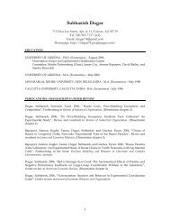
We close this brief data section by providing the reader with a sense of the variation in the
evolution of prices across regions of the Bay Area. The precision of our model depends critically
on the fact that rates of house price appreciation are not uniform across neighborhoods. Figure
1 reports real house price appreciation by PUMA from 1990 to 2004. The estimated price levels
are derived separately for each PUMA using a repeat sales analysis in which the log of the sales
12

Figure 3: Ground-Level Ozone (Days Exceeding State Limit)
Table 4: Time-Series Properties of Bay Area Amenities
Violent Crime Ground-Level Ozone Percentage White
AR(1) Coefficient .718 -.057 1.026
S.E. (.012) (.022) (5.18x10-3)
Obs 2250 2250 2250
R 2 .6177 .0030 .9459
Note: Variables are demeaned at the neighborhood level
price (in 2000 dollars) is regressed on a set of year fixed effects as well as house fixed effects.
The figure reveals significant differences across PUMAs in real house price growth over this time
period
3 A Dynamic Model of Neighborhood Choice
Previous work on the sorting of households across neighborhoods has universally adopted a
static approach. 10 We introduce the dynamics of the neighborhood choice problem through
10 See Epple and Sieg (1999), Bayer McMillan and Rueben (2004), Ferreyra (2006), Ekeland, Heckman, and
Nesheim (2004) and Bajari and Kahn (2005) for some important recent examples. Two exceptions are Kennan
and Walker (2005) and Bishop (2007), which analyze interregional migration in the US in a dynamic context.
Murphy (2007) examines the role of dynamic behavior is the supply of new housing.
13

Figure 4: Violent Crimes (per 100,000 residents)
two channels: wealth accumulation, and moving costs. Households have expectations about
appreciation of housing prices and may rationally choose a neighborhood that offers lower current
period utility in return for the increase in wealth that would accompany price increases in that
neighborhood. The other component of the neighborhood choice problem that induces forward
looking behavior on the part of households are moving costs. Because households typically pay
5-6 percent of the value of their house in real estate agent fees in addition to the non-financial
costs of moving, it is prohibitively costly to re-optimize every period. As a result, households
will naturally consider expectations of the future utility streams when deciding where to live.
Therefore, households likely make trade-offs between current and future neighborhood attributes,
choosing neighborhoods based in part on demographic or economic trends.
We model households as making a sequence of location decisions that maximize the dis-
counted sum of expected per-period utilities. Our general model can be formulated in a familiar
dynamic programming setup, where a Bellman equation illustrates the determinants of the op-
timal choice. We model households as choosing between neighborhoods. As discussed in the
data section, each neighborhood has approximately 10,000 houses and is created by combining
U.S. Census tracts. Our data for the San Francisco Bay Area includes information on over
one million house sales in 225 neighborhoods between 1990 and 2004. In each period, every
14

Figure 5: Appreciation rates by neighborhood
Appreciation
Marin
San Francisco
47 - 50
51 - 55
56 - 58
59 - 60
61 - 65
66 - 72
73 - 81
82 - 125
San Mateo
Contra Costa
Alameda
Santa Clara
household chooses whether to move or not. If the household moves, it incurs a moving cost and
then chooses the neighborhood that yields the highest expected lifetime utility.
A key feature of our approach is that it controls for unobserved neighborhood heterogeneity
in a dynamic model using a semi-parametric estimator that is computationally tractable. The
model, as outlined below, is one of homeowner behavior and does not consider the decision
whether to rent or to own.
The observed state variables at time t are Xjt, Zit, and dit−1. Xjt is a vector of characteristics
of the different choice options that affect the per period utility a household may receive from
choosing neighborhood j ∈ {1, . . . , J}. Zit is a vector of characteristics of each household that
potentially determine the per period utility from living in a particular neighborhood, as well
as the costs associated with moving. For example, X may include variables such as price of
housing, quality of local attributes such as air quality, crime, or the racial composition in the
neighborhood. Z may include such variables as income, wealth, or race.
The decision variable, dit, is given by the function dit = d(·) where the arguments of d(·) are
discussed below. dit, denotes the choice of household i in period t. Therefore, in the context
of our model, the state variable, dit−1, is the neighborhood in which household i resides before
15

making a decision in period t.
In addition to the decision variable, d, and the observable variables, Xjt, Zit, and dit−1,
there are three unobservable variables, ξjt, ɛijt, and ζit. We include and control for unobserved
neighborhood characteristics, ξjt. 11 ɛijt is an idiosyncratic stochastic variable that determines
the utility a household receives from living in neighborhood j in period t, and ζit is an idiosyn-
cratic shock to moving costs that also varies by period. We assume for simplicity that ζit is
the same for all j. Let Ωt denote an information set which includes all current characteristics,
{Xjt, ξjt} J j=1 and anything that helps predict future characteristics. Let sit denote the states
Ωt, Zit, and dit−1.
The primitives of the model are (u, MC, q, β). uijt = u(Xjt, ξjt, Zit, ɛijt) is the per period
utility function excluding any moving costs that household i receives from choosing neighbor-
hood j. MCit = MC(Zit, Xdit−1t, ζit) is the per period moving cost function, which are are only
paid when a household moves. By assumption, they are not determined by where a household
moves to. However, they are a function of the characteristics of the neighborhood the house-
hold is leaving, Xdit−1t, to capture the fact that realtor fees are proportional to the house one
sells. The full flow utility function is given by u MC
ijt = uijt − MCitI [j�=dit−1]. The transition
probabilities of the observables and unobservables are assumed to be Markovian and are given
by q = q(sit+1, ζit+1, ɛit+1|sit, ζit, ɛit, dit). Finally, β is the discount factor.
Each household is assumed to behave optimally in the sense that its actions are taken to
maximize lifetime expected utility. That is, the problem of the household is to choose a sequence
of decisions, {dit}, to maximize:
E � T �
r=t
β r−t� u MC (Xjr, ξjr, Zir, ɛijr, Xdir−1r, ζir) �� �
�sit, ζit, ɛit, dit
d ∗ is the optimal decision rule and under the Markov structure of the problem is only a
function of the state variables. That is, dit = d ∗ it (sit, ζit, ɛit). When the sequence of decisions,
{dit}, is determined according to the optimal decision rule, d ∗ , lifetime expected utility becomes
11 We differ from previous work, such as Berry, Levinsohn, and Pakes (1995), that forces all individuals to
have the same preferences for the unobserved neighborhood characteristic by allowing individuals to value the
unobserved neighborhood characteristic differently depending on their demographic characteristics. In practice,
different neighborhood unobservables will be specified for different types of individuals.
16
(1)

the value function. We can break out the lifetime sum into the flow utility at time t and the
expected sum of flow utilities from time t + 1 onwards. This allows us to use the Bellman
equation to express the value function at time t as the maximum of the sum of flow utility at
time t and the discounted value function at time t + 1. We assume that the problem has an
infinite horizon allowing us to drop the time subscripts on V , the value function. 12
V (sit, ζit, ɛit) = maxj{u MC
ijt + βE � V (sit+1, ζit+1, ɛit+1) � � sit, ζit, ɛit, dit = j � } (2)
Under certain technical assumptions, equation (2) is a contraction mapping in V . How-
ever, the difficulty is that V is a function of both the observed and unobserved state variables.
Therefore, we make a series of assumptions similar to those in Rust (1987) which simplify the
model.
Assumption (AS): Additive Separability. We assume that the per period utility function, u,
is additively separable in the idiosyncratic error term, ɛijt. Therefore we can express the full
flow utility function, u MC
ijt , as
u MC
ijt = u(Xjt, ξjt, Zit) − MC(Zit, Xdit−1t, ζit)I [j�=dit−1] + ɛijt (3)
Assumption (CI): Conditional Independence. We make the following assumptions regarding
the transition probabilities of the observed and unobserved states. The idiosyncratic neigh-
borhood error term, ɛijt is distributed i.i.d. Type 1 Extreme value (with density qɛ) and the
idiosyncratic moving error term, ζit is distributed i.i.d. Normal (with density qζ). Additionally,
we assume that conditional on s and j, the errors ɛijt and ζit have no predictive power about
future states s. We can therefore express the transition density for the Markov process, q, as 13
q(sit+1, ζit+1, ɛit+1|sit, ζit, ɛit, dit) = qs(sit+1|sit, dit)qζ(ζit+1)qɛ(ɛit+1) (4)
This allows us to define the choice specific value function, vMC j (sit, ζit).
12 Assuming an infinite horizon implies Vt(sit, ζit, ɛit) = V (sit, ζit, ɛit) and dt(sit, ζit, ɛit) = d(sit, ζit, ɛit).
13 In the section on estimation, we will outline in detail our assumptions about the transitions of the observable
states.
17

v MC
�
j (sit, ζit) = uijt − MCitI [j�=dit−1] + βE
where
log � J �
k=1
log � J �
k=1
exp(v MC
k (sit, ζit)) � �
� �
= Eɛ V (sit, ζit, ɛit) = Eɛ
exp(v MC
k (sit+1, ζit+1)) �� �
�
�sit, dit = j
maxk[v MC
k
�
(sit, ζit) + ɛikt]
Similarly to the per-period utility, we break out the full choice specific value function into a
component capturing the lifetime expected utility of choosing neighborhood j ignoring moving
costs and another component involves moving costs.
4 Estimation
v MC
j (sit, ζit) = vj(sit) − MC(Zit, Xdit−1t, ζit)I [j�=dit−1] (6)
�
vj(sit) = uijt + βE log � J �
exp(v MC
k (sit+1, ζit+1)) �� �
�
�sit, dit = j
k=1
The estimation of the primitives of the model proceeds in four stages. In the first stage, we
recover the non-moving cost component of lifetime expected utility. In the second stage, we
recover moving costs. We also recover an estimate of the marginal utility of wealth. While
a number of standard options for estimating the marginal utility of wealth are available, we
identify the marginal utility of wealth by utilizing outside information on the financial costs of
moves. Having recovered moving costs and the marginal utility of wealth in the second stage, we
recover fully flexible estimates of the per-period utility in the third stage. With estimates of the
per-period utility function, it is straightforward to decompose per-period utility as a function
of observable states in the fourth stage. A key feature of our estimation strategy is its low
computational burden.
18
(5)
(7)

4.1 Estimation Stage One - Choice Specific Value Function
Consider the problem faced by a household that has chosen to move. It will choose a neigh-
borhood which offers the highest lifetime utility by maximizing over the choice specific value
functions v MC . However, conditional on moving, the moving cost term, MC(Zit, dit−1, ζit), is
assumed to be identical for all neighborhoods. As an additive constant, it simply drops out
and, conditional on moving, each household chooses j to maximize vj(sit) + ɛijt, where vj(sit) is
given in (7)
We have assumed that the idiosyncratic error term, ɛijt, is distributed i.i.d., Type 1 Extreme
Value, which allows us to recover vj(sit) in a number of ways. Previous methods for estimating
dynamic discrete choice models in the presence of a large choice set are plagued by a curse
of dimensionality. We therefore employ a variant of Hotz and Miller (1993) based on the
contraction mapping in Berry (1994) which avoids this problem. Specifically, based on household
characteristics such as income, wealth, and race, we divide households into distinct types indexed
by τ. Let θ τ jt = vj(sit) when the characteristics of the household i (Zit) imply that the household
is of type τ. θ τ jt
is then the choice-specific value a household of type τ receives from choosing
neighborhood j, ignoring any potential moving costs. Let δ τ jt
denote the deterministic component
of flow utility for a household of type τ. We can rewrite (7) using lifetime utilities, θ τ jt .
θ τ jt = δ τ �
jt + βE log
� J �
k=0
exp(θ τt+1
kt+1 − MCτt+1
jt+1I �� �
��sit,
[k�=j]) dit = j
Household i of type τ chooses neighborhood j if θ τ jt + ɛijt > θ τ kt + ɛikt∀k �= j. Conditional upon
moving, the probability of any household of type τ choosing neighborhood j in period t when
ɛijt is distributed i.i.d., Type 1 Extreme Value can therefore be expressed as:
P τ jt(θ τ t ) =
e θτ jt
� J
k=1 eθτ kt
For any given time period, the vector of mean lifetime utilities, θ τ t , is unique up to an additive
constant, thus requiring some normalization for each τ. We temporarily normalize the mean
(over neighborhoods) of the fixed effects to zero for each type in each time period. Denoting the
number of types as M implies that, in each time period, we make M normalizations. Therefore,
19
(8)
(9)

instead of recovering θ τ jt for every neighborhood and type, we recover ˜ θ τ jt where ˜ θ τ jt = θτ jt − mτ t
and m τ t = 1/J �
j θτ jt . Let ˆ P τ jt
denote the estimated probability of households of type τ who
choose in neighborhood j in period t. We can then easily calculate ˜ θ τ jt as:
˜θ τ jt = log( ˆ P τ jt) − 1/J �
k
log( ˆ P τ kt ) (10)
As the number of types, M, grows large relative to the sample size, we may face some small
sample issues with observed shares. Therefore, instead of simply calculating observed shares
as the portion of households of a given type who live in an area, we use a weighted measure to
avoid zero shares. We do this to incorporate the information from similar types when calculating
shares for any particular type. For example, if we want to calculate the share of households
with an income of $50,000 choosing neighborhood j in period t, we would use some information
about the residential decisions of those earning $45,000 or $55,000 in that period. Naturally,
the weights will depend on how far away the other types are in type space. We denote the
weights by W τ (Zit). The formula for calculating observed shares is given by: 14
ˆP τ jt =
� N
i=1 I [di=j] · W τ (Zit)
� N
i=1 W τ (Zit)
where the weights are constructed as the product of K kernel weights, where K is the dimension
of Z. Each individual kernel weight is formed using a standard normal kernel, N, and bandwidth,
hk, determined by visual inspection.
K�
W τ (Zit) =
hk
k=1
(11)
1
N( Zit − Zτ ) (12)
4.2 Estimation Stage Two - Moving Costs and the Marginal Utility of Wealth
Households behave dynamically by taking into account the effect their current decision has on
future utility flows. In our model, the current decision affects future utility flows through two
channels. Households are aware they will incur a transaction cost by re-optimizing in the future.
In addition, the decision about where to live today affects wealth in the future. Equation (8)
14 If W τ (Zi) = I[Z i=Z τ ], this results in the simple cells estimator for calculating shares/probabilities.
20
hk

shows how the current action impacts both today’s flow utility and the future utility. It also
suggests that if θτ jt (or ˜ θτ jt ) is known for all τ and j, we can estimate moving costs based on
households decisions to move or stay in a given period.
Given estimates of ˜ θ τ jt
from the first stage, we can estimate moving costs in stage two by
considering the move/stay decisions of households. From the model outlined above, we know
that in any given period a household will move if the lifetime expected utility of staying in their
current neighborhood is less than the lifetime expected utility of the best other alternative when
moving costs are factored in.
The issue of an outside option arises here. If a household chooses to move, they do not have
to move to another neighborhood in the Bay Area. We therefore want to include a lifetime
utility term for an outside option. Our data allows us to follow individuals through time, which
means we can calculate the probability (in each year) that a seller leaves the Bay Area. We use
this procedure in combination with the estimated probabilities of choosing the inside options to
get a normalized lifetime utility of choosing the outside options for each type. We denote this
lifetime utility as ˜ θ τ 0
and include it the set of alternatives in the move/stay decision.
We assume that moving costs, MC τt
jt , are comprised of financial costs, F MC(dit−1) and psy-
chological costs, P MC(Zit, ζit). The financial moving costs are a function of dit−1 as households
pay financial costs based primarily on the property the sell. The psychological costs are a func-
tion of the observable characteristics, Zit, that define type τ as well as the unobserved stochastic
component, ζit.
As the financial moving costs reduce wealth, choosing to move changes a households type.
For example, if moving costs are $10,000, then a given household with $100,000 in wealth chooses
where to live based on the utility of staying in their current neighborhood with wealth of $100,000
and the highest alternative utility with a wealth of $90,000. In practice, we treat financial moving
costs as observable and set them equal to 6% of the value of housing in the neighborhood a
household is leaving (i.e., F MC = 0.06 · P ricedit−1 ).
If a household of type τ living in neighborhood j moves, we denote their new type as ¯τj. The
new type following a move reflects the reduction in wealth by the amount of F MC.
21

A household who chose dit−1 = j will choose to stay if:
Maxk�=j[θ ¯τjt
kt + ɛikt] − P MC(Zit, ζit) < θ τ jt + ɛijt (13)
However, from the first stage we only recover the demeaned choice specific value functions,
˜θ τ j , where ˜ θ τ j = θτ j − mτ . We can then rewrite (13) as:
Maxk�=j[ ˜ θ ¯τjt
kt + ɛikt] − (m τ t − m ¯τjt
t ) − P MC(Zit, ζit) < ˜ θ τ jt + ɛijt (14)
The term m τ t − m ¯τjt
t is unobserved but can be estimated. Recall that m τ t = 1/J �
j θτ jt and,
as such, m τ t − m ¯τjt
t is the difference (averaged across neighborhoods) between having the utility
associated with being type τ and the having the utility from the reduced wealth after paying the
financial moving costs. In principle, we could estimate a separate term for each combination of
τ and F MC, however, we choose to parameterize it as a function of Zit and F MCit.
We also parameterize the psychological costs
m τ t − m ¯τjt
t = F MCitγ τ fmc
F MCit = 0.06 · P ricedit−1
γ τ fmc = Z′ itγfmc
P MCit = Z ′ itγpmc + ζit
Note that the three stochastic terms are Maxk�=j[ ˜ θ ¯τjt
kt + ɛikt], ɛijt, and ζit. We estimate
m τ t −m ¯τjt
t and P MCit from a likelihood function based on the probability of a household staying
in its current house
P τ
� ∞
it(Stay|dit−1 = j) =
−∞
e ˜ θ τ jt
e ˜ θ τ jt + �
k�=j e˜ θ ¯τ jt
kt −F MCitγ τ fmc −Z′ it γpmc−ζit
· φ(ζit)d(ζit) (15)
We then use equation (15) to form a likelihood equation based of every households’ move/stay
decision in every period. Maximizing this likelihood will yield estimates of γfmc and γpmc
22

The earlier (first) stage of our estimation approach involved making a normalization for each
type of household (i.e., ˜ θ τ jt
is mean zero across all locations j), where type could be defined by
personal characteristics such as race, income, wealth. Once we set the mean choice specific utility
from no wealth to zero, we only need to know these baseline differences, m τ t − m ¯τjt
t , to recover
the unnormalized choice specific value functions. As we can estimate the baseline differences,
we can simply recover the true choice specific value functions as θ τ jt = ˜ θ τ jt + mτ t .
It is important to recover these baseline differences because they represent the extra utility
a household would receive from extra wealth. A key aspect of the dynamic model is that the
choice of neighborhood affects future type. Therefore, the baseline differences in utility across
types represent potential future utility gains from wealth accumulation.
4.3 Estimation - Stage Three - Per-Period Utility
From stages one and two, we know the distribution of moving costs for each type, the marginal
value of changing type, and the true mean utility terms, θτ j . The next step is to specify and
estimate transition probabilities.
We assume that households use today’s states to directly predict future values of the lifetime
utilities, θ, rather than predicting the values of the variables upon which θ depends. As potential
future moving costs are a function of the price of housing in the neighborhood chosen in this pe-
riod, households need to predict how the price of the house they currently occupy will transition.
Finally, as both moving costs and lifetime utilities are determined by type, households need to
predict how their types will change. The only determinant of type that changes endogenously is
wealth. We assume that knowing how house prices transition is sufficient for knowing how wealth
(and therefore type) transition. 15 We therefore only need to model transition probabilities for
θ and price.
The nature of the housing market imposes certain simplifications on the transition probabil-
ities. The current period’s decision, dit, can have no bearing on how neighborhood utilities, θ,
or prices transition. The current period’s decision, dit, the current period’s type, τit, and the
transition probabilities for housing prices are sufficient for predicting next period’s type, τit+1.
15 With access to richer data about other forms of household wealth, the definition of wealth that we use to
define type could be expanded.
23

In theory, we could estimate the θ transition probabilities separately by type, as we have a
time series for each type and neighborhood. However, to increase the efficiency of our estimates,
we impose some restrictions. For example, within each type we could assume that the neigh-
borhood mean utilities, θτ jt , evolve according to an auto-regressive process where some of the
coefficients are common across neighborhoods. In practice, we estimate transition probabilities
separately for each type but pool information over neighborhoods. To account for different means
and trends we include a separate constant and time trend for each neighborhood’s choice specific
value function for each type. We model the transition of the choice specific value functions, θ τ jt ,
as:
θ τ jt = ρ τ 0,j +
L�
l=1
ρ τ 1,l θτ jt−l +
L�
l=1
Xjt−l′ρ τ 2,l + ρτ 3,j t + ω τ jt
where the time varying neighborhood attributes included in Xjt are price, racial composition
(percentage white), pollution (number of days ozone concentration exceed the California state
maximum threshold), and the violent crime rate. 16
We also need to know how housing wealth transitions in order to specify transition probabili-
ties for types. We use sales data to construct price indexes for each type, tract, year combination.
Recalling that price is one of the variables in X, we estimate transition probabilities on price
levels according to:
pricejt = ϱ0,j +
L�
l=1
Xjt−l′ϱ2,l + ϱ3,j t + ϖ τ jt
Given transition probabilities on price levels it is straightforward to estimate transition prob-
abilities for wealth and type, τ. In both cases, we use two lags of the dependent variable (θ τ jt or
priceτ jt ) as well as two lags of the other exogenous variables in X.
Knowing θ, P MC, and the transition probabilities allows us to calculate mean flow utilities
for each type and neighborhood, δτ jt , according to:
δ τ jt = θ τ �
jt − βE log
� J �
k=0
exp(θ τt+1
kt+1 − MCτt+1
jt+1I �� �
��sit,
[k�=j]) di,t = j
where in practice, s includes all the variables on the right hand side of equations (16) and (17)
16 For the outside option, we don’t observe any attributes and we estimate with only lags of the choice specific
value function. That is, we estimate θ τ 0t = ρ τ 0,0 + � L
l=1 ρτ 1,lθ τ 0t−l + ρ τ 3,0 t + v τ 0t
24
(16)
(17)
(18)

For each type, τ, neighborhood, j, and time, t, we have the necessary information to simulate
the expectation on the right hand side of (18). To do this we draw a large number of ζt+1, θt+1
and pricet+1 according to their estimated distributions. Using r to index random draws, each
ζt+1(r) is drawn from a normal distribution with a variance equal to that estimated in Stage
2. θt+1(r) and pricet+1(r) are generated by drawing from the empirical distribution of errors
obtained when estimating (16) and (17) and using the observed values of the current states. The
draws on pricet+1 are used to form τt+1 and MC τt+1
a δ τ jt (r). The simulated δτ jt
is then calculated as 1
R
recover the M · J · T values for the mean flow utilities, δ τ jt
jt+1 .17 For each draw, r, we can then calculate
�R r=1 δτ jt (r). It is then straightforward to
using (18)
4.4 Estimation - Stage Four - Decomposing Per-Period Utility
Once we recover the mean per-period flow utilities, we can decompose them into functions of
the observable neighborhood characteristics, Xjt. We treat ξjt as an error term in the following
regression.
δ τ jt = g(Xjt; α) + ξ τ jt
g(Xjt; χ) is a function of Xjt known up to parameter vector α. This decomposition of the
mean flow utilities is similar to Berry, Levinsohn, and Pakes (1995) or Bayer, McMillan, and
Rueben (2004). However, in these models the neighborhood unobservable, ξjt, was a vertical
characteristic that affected all households utility in the same way. In our application, we are more
flexible and allow households who are different, based on observable demographic characteristics,
to view the unobservable component differently as in Timmins (2007); hence the τ superscript
on ξ τ jt .
In principal, we could decompose the flow utilities separately for each type, τ. However,
in practice we use the following specification to decompose the type specific flow utilities. In
addition to neighborhood characteristics, we include dummies for type (τ), county (c), and year
(t). 18
δ τ jt = ατ + αc + αt + X ′ jtαx + ξ τ jt
17 Once we draw a value for pricet+1 we can calculate wealtht+1 as pricet+1-mortgageamount and MC τ t+1
jt+1 as
6% of pricet+1.
18 In principal, we could also interact the neighborhood and year dummies with type.
25
(19)
(20)

The time varying characteristics used in our application are rent, ground-level ozone (mea-
sured in days exceeding the state standard), violent crime (measured in incidents per 100,000
residents), and a measure of racial composition (percentage white).
Rent (or user cost of owning a house) is typically calculated as a percentage of house value.
We calculate neighborhood rent as 5% of a mean prices in the neighborhood. Rents, however,
are clearly endogenous. The traditional approach to solving this problem is to use instrumental
variables. Our approach to this problem is different. We use the estimate of the marginal utility
of wealth found in Section 4.2 to recover the marginal disutility of rent. We assume that the effect
of a marginal change in wealth on lifetime utility is the same as the effect of a marginal change
in income on one period’s utility. In particular, the marginal utility of income (the negative of
which can be interpreted as the coefficient on rent) is given by γτ fmc . Therefore we estimate the
following regression where �γ τ fmc is known from Stage 2 and ˜ X denotes the non-rent components
of X.
5 Results
δ τ jt + �γ τ fmc rentjt = ατ + αc + αt + ˜ X ′ jtαx + ξ τ jt
The following section reports results. We estimate the model for whites only. The process could,
however, be easily replicated for other racial groups, although small number problems may be
more binding in first stage for minorities. Without an explicit analysis of the value of racial
composition, racial groups could simply be pooled. We had 625 types, where types were defined
by wealth and income, which were measured in $10,000 increments $0 to $240,000.
5.1 Moving Costs and the Marginal Utility of Wealth
In the second stage of estimation, the binary move/stay decision made every period was used
to identify and estimate both psychological and financial moving costs. Using the outside infor-
mation that financial moving costs are 6% of the selling price allows us to recover the marginal
utility of wealth. The results of the second stage estimation are given in Table 5.
26
(21)

Table 5: Moving Cost Estimates
Estimate Standard Error
Psychological Costs
Constant 9.3340 0.0226
Income -0.0035 0.0002
Tenure
Financial Costs
-0.0760 0.0019
Constant*6% House Value 0.02458 0.00093
Income*6% House Value -0.00006 0.000006
Note: Income and House Value are measured in $1000.
Note: Standard Errors do not account for first stage estimation.
5.2 Marginal willingness to pay for neighborhood attributes
We decompose the estimates of the flow utilities using our strategy for controlling for the endo-
geneity of rent by estimating equation (21). Table 6 reports these results.
Table 6: Decomposition of flow utilities
δ τ jt + �γ τ fmc rentjt
Coefficient Standard Error
%white .0028 .00003
.01*violent crime rate -.0027 .00002
ozone -.0104 .00018
County Dummies Yes
Year Dummies Yes
Type Dummies Yes
Note: Standard Errors do not account for first stage estimation.
To understand the magnitude of these coefficients, we can calculate willingnesses to pay for
changes in each of the neighborhood characteristics. Marginal willingness to pay (in $1000s) is
given by αx/γτ fmc . To better illustrate the results, Table 7 reports the willingness to pay (WTP)
for a 10% change in each amenity. The willingness to pay figures are reported at the means of
%white (69), violent crime rate (437), and ozone (2.28) as well as at the mean household income
27

of $114,368.
Table 7: Willingness to Pay for 10% increase in Amenities
MW T P
%white $1076.56
violent crime rate -$655.99
ozone -$155.58
6 Dynamic versus Static Approaches
Equation (8) illustrates the problems associated with estimating a static model when the true
model is dynamic. Specifying a static model creates an omitted variables problem. Current
neighborhood characteristics determine the choice specific value functions in two ways: they
affect the flow utility directly and they help predict future neighborhood utility. Estimating a
static model omits the second effect.
The nature of how current characteristics predict future utility will determine whether the
static estimator over-predicts or under-predicts the effect of the characteristic on utility. For
example, if high pollution today predicts falling pollution tomorrow, then we would expect the
static model to understate the disutility of pollution. This is, in fact, the pattern we see over
time in our data describing both ground-level ozone and violent crime. The argument is simple
– households may be willing to pay quite a bit to avoid high levels of air pollution or crime.
However, when they see a neighborhood with low values of one of these disamenities, they know
that value will rise in the future; they are therefore less willing to pay as much for a house in
that neighborhood as they would be if the low value were permanent. Transitory amenities
are simply not worth as much. A naive hedonic model ignores this fact and takes households’
behavior as evidence that the low values of the disamenity aren’t actually worth that much.
In contrast, there are other neighborhood attributes that are persistent over time (e.g., racial
composition). In contrast to ozone and crime, seeing a high value of “percentage white” today
signals that the neighborhood is likely to remain high percentage white in the future. If this
is an attribute that households value (recall that we are only modeling the decisions of white
28

household heads in the current application), they will be willing to pay more for a house in
such a neighborhood than they would if the high value of the attribute were only temporary.
Persistent amenities are worth more than fleeting ones. A naive static model ignores this fact
and attributes all of the value to current preferences, overstating the contribution to flow utility
of high percentage white neighborhoods to white households.
An additional issue that affects how the the static model could bias estimates of the utility
parameters is the fact even if the researcher were to incorrectly assume the model to be static, she
would still need to control for the fact that price and the unobserved neighborhood attributes are
likely correlated. A typical approach is to use an instrumental variables strategy. The problem
with this approach is that, if the underlying model really is dynamic, any static instrument will
be correlated with expected future utility, which is subsumed in the error term. A condition
of any potential instrument is that it is correlated with price. The expected future utility is
a function of current attributes, therefore, unless current price has no predictive power about
future utility, it is impossible to find an instrument that is correlated with price but not correlated
with expected future utility.
To highlight the problems with ignoring forward looking behavior, we also estimate a static
version of our model. Under the assumption that agents are not forward looking, Stage 1
estimates (i.e., θτ jt ) can be interpreted as flow utilities. We can then decompose them by
running the same Stage 4 procedure. In particular, we estimate equation (21), replacing δ τ jt with
θτ jt . Table 8 reports the marginal willingness to pay for a 10% change in each amenity from that
model. The dynamic results shown in Table 7 are also included to make comparison easier. As
before, the marginal willingness to pay figures are reported at the means of the amenities and
income.
Table 8: Willingness to Pay for 10% increase in Amenities
MW T P
Static Dynamic
%white $1850.22 $1076.56
violent crime rate -$554.63 -$655.99
ozone -$91.28 -$155.58
29

The comparison of static and dynamic results suggests that incorrectly estimating a static
model can lead to estimates with very large biases. In our application a static model substantially
overestimated willingness to pay to live with other white neighbors. However, the bias for ozone
and crime, while also large, runs in the opposite direction (in absolute terms).
7 Conclusion
We develop a tractable model of neighborhood choice in a dynamic setting along with a compu-
tationally straightforward estimation approach. We estimate the model using a novel data set
that links buyer and seller demographics to detailed house characteristics. We use the dynamic
model to recover estimates of moving costs and the marginal willingness to pay for neighborhood
attributes and compare these results with an alternative static estimator to explain the biases
associated with static approaches. The model and estimation approach are applicable to the
study of a wide set of dynamic phenomena in housing markets and cities. These include, for
example, the analysis of the microdynamics of residential segregation and gentrification within
metropolitan areas.
30

References
Abraham, J., and P. Hendershott (1996): “Bubbles in Metropolitan Housing Markets,”
Journal of Housing Research, 7(2), 191–207.
Bajari, P., C. L. Benkard, and J. Krainer (2005): “House Prices and Consumer Welfare,”
Journal of Urban Economics, 58, 474–487.
Bajari, P., and M. Kahn (2005): “Estimating Housing Demand With An Application to
Explaining Racial Segregation in Cities,” Journal of Business and Economic Statistics, 23(1),
20–33.
Bayer, P., F. Ferreira, and R. McMillan (2007): “A Unified Framework for Measuring
Preferences for Schools and Neighborhoods,” mimeo, Duke University.
Bayer, P., and R. McMillan (2006): “Racial Sorting and Neighborhood Quality,” NBER
Working Paper No. 11813.
Bayer, P., R. McMillan, and K. Rueben (2004): “An Equilibrium Model of Sorting in an
Urban Housing Market,” NBER Working Paper No. 10865.
Bayer, P., and C. Timmins (2005): “On the Equilibrium Properties of Locational Sorting
Models,” Journal of Urban Economics, 57, 462–477.
(2007): “Estimating Equilibrium Models of Sorting Across Locations,” Economic Journal,
Forthcoming.
Berry, S. (1994): “Estimating Discrete Choice Models of Product Differation,” Rand Journal
of Economics, 25, 242–262.
Berry, S., J. Levinsohn, and A. Pakes (1995): “Automobile Prices in Market Equilibrium,”
Econometrica, 63, 841–890.
Bishop, K. (2007): “A Dynamic Model of Location Choice and Hedonic Valuation,” working
paper, Washington University in St. Louis.
Capozza, D., P. Hendershott, C. Mack, and C. Mayer (2002): “Determinants of Real
House Price Dynamics,” NBER Working Paper No. 9262.
Card, D., A. Mas, and J. Rothstein (2006): “Tipping and the Dynamics of Segregation in
Neighborhoods and Schools,” mimeo.
Carranza, J. E. (2007): “Estimation of demand for dierentiated durable goods,” mimeo.
Case, K., and C. Mayer (1995): “Housing Price Dynamics within a Metropolitan Area,”
NBER Working Paper No. 5182.
31

Case, K., and R. Shiller (1989): “The Efficiency of the Market for Single-Family Homes,”
American Economic Review, 79(1), 125–137.
Cho, M. (1996): “House Price Dynamics: A Survey of Theoretical and Empirical Issues,”
Journal of Housing Research, 7(2), 145–172.
Clayton, J. (1997): “Are Housing Prices Driven by Irrational Expectations?,” Journal of Real
Estate Finance and Economics, 14(3), 341–63.
Cutler, D., E. Glaeser, and J. Vigdor (1999): “The Rise and Decline of the American
Ghetto,” Journal of Political Economy, 107, 455–506.
Easterly, W. (2004): “Empirics of Strategic Interdependence: The Case of the Racial Tipping
Point,” NYU Development Research Working Paper No. 5.
Ekeland, I., J. J. Heckman, and L. Nesheim (2004): “Identification and Estimation of
Hedonic Models,” Journal of Political Economy, 112(1), S60–S109.
Ellison, G., and E. Glaeser (1997): “Geographic Concentration in U.S. Manufacturing
Industries: A Dartboard Approach,” Journal of Political Economy, 105(5), 889–927.
Englund, P., T. Gordon, and J. Quigley (1999): “The Valuation of Real Capital: A
Random Walk down Kungsgatan,” Journal of Housing Economics, 8, 205–216.
Epple, D., and H. Sieg (1999): “Estimating Equilibrium Models of Local Jurisdictions,”
Journal of Political Economy, 107, 645–681.
Erdem, T., S. Imai, and M. P. Keane (2003): “Brand and Quantity Choice Dynamics Under
Price Uncertainty,” Quantitative Marketing and Economics, 1(1), 5–64.
Fan, J. (1992): “Design-Adaptive Non-Parametric Regression,” Journal of the American Statistical
Assosciation, 87(420), 998–1004.
Ferreyra, M. (2007): “Estimating the Effects of Private School Vouchers in Multi-District
Economies,” American Economic Review, Forthcoming.
Gelfand, A., M. Ecker, J. Knight, and C. Sirmans (2004): “The Dynamics of Location
in Home Price,” Journal of Real Estate Finance and Economics, 29(2), 149–166.
Gibbons, S. (2004): “The Costs of Urban Property Crime,” The Economic Journal, 114, F441–
F463.
Glaeser, E., and J. Gyourko (2007): “Housing Dynamics,” mimeo.
Gowrisankaran, G., and M. Rysman (2006): “Dynamics of Consumer Demand for New
Durable Goods,” mimeo.
32

Hendel, I., and A. Nevo (2006): “Measuring the Implications of Sales and Consumer Inventory
Behavior,” Econometrica, 74(6), 1637–1673.
Himmelberg, C., C. Mayer, and T. Sinai (2005): “Assessing High House Prices: Bubbles,
Fundamentals, and Misperceptions,” Journal of Economic Perspectives, 19(4), 67–92.
Hotz, V. J., and R. A. Miller (1993): “Conditional Choice Probabilities and the Estimation
of Dynamic Models,” Review of Economic Studies, 60, 497–529.
Hotz, V. J., R. A. Miller, S. Sanders, and J. Smith (1994): “A Simulation Estimator for
Dynamic Models of Discrete Choice,” Review of Economic Studies, 61, 265–289.
Kennan, J., and J. R. Walker (2005): “The Effect of Expected Income on Individual Migration
Decisions,” NBER Working Paper No. 9585.
Lamont, O., and J. Stein (2004): “Leverage and House-Price Dynamics in U.S. Cities,”
mimeo, University of Chicago GSB.
McCarthy, J., and R. Peach (2004): “Are Home Prices the Next Bubble?,” Economic Policy
Review, 10(3), 1–17.
Melnikov, O. (2001): “Demand for Differentiated Durable Products: The Case of the U.S.
Computer Printer Market,” mimeo.
Merlo, A., F. Ortalo-Magné, and J. Rust (2006): “Models of Bargaining and Price Determination
of Residential Real Estate, with and without Real Estate Agents,” mimeo.
Murphy, A. (2007): “A Dynamic Model of Housing Supply,” working paper, Washington
University in St. Louis.
Ortalo-Magné, F., and S. Rady (1999): “Boom In, Bust Out: Young Households and the
Housing Price Cycle,” European Economic Review, 43, 755–766.
(2005): “Heterogeneity Within Communities: A Stochastic Model with Tenure Choice,”
CESifo Working Paper No. 1465.
(2006): “Housing Market Dynamics: On the Contribution of Income Shocks and Credit
Constraints,” Review of Economic Studies, 73(2), 459–485.
Roback, J. (1982): “Wages, Rents, and the Quality of Life,” Journal of Political Economy,
90(6), 1257–1278.
Rosenthal, S. (1999): “Residential Buildings and the Cost of Construction: New Evidence on
the Efficiency of the Housing Market,” Review of Economics and Statistics, 81(2), 288–302.
33

Rust, J. (1987): “Optimal Replacement of GMC Bus Engines: An Empirical Model of Harold
Zurcher,” Econometrica, 55(5), 999–1033.
(1994): “Structural Estimation of Markov Decision Processes,” in Handbook of Econometrics,
ed. by R. Engle, and D. McFadden, vol. 4. New York: North Holland.
Schelling, T. (1971): “Dynamic Models of Segregation,” Journal of Mathematical Sociology,
pp. 143–186.
Schiraldi, P. (2006): “Automobile Replacement: A Dynamic Structural Approach,” mimeo,
Boston University.
Shiller, R. (2005): Irrational Exuberance. Princeton University Press, 2nd edn.
(2006): “Long-Term Perspectives on the Current Boom in Home Prices,” The
Economists’ Voice, 3(4), Article 4.
Timmins, C. (2006a): “Estimable Equilbrium Models of Locational Sorting and Their Role in
Development Economics,” Journal of Economic Geography, 5, 83–100.
(2006b): “Estimating Spatial Differences in the Brazilian Cost-of-Living With Household
Location Chocies,” Journal of Development Economics, 80(1), 59–83.
(2007): “If You Can’t Take the Heat, Get Out of the Cerrado... Recovering the Equilibrium
Amenity Cost of Non-Marginal Climate Change in Brazil,” Journal of Regional Science,
Forthcoming.
Timmins, C., and J. Murdock (2007): “A Revealed Preference Approach to the Measurement
of Congestion in Travel Cost Models,” Journal of Environmental Economics and Management,
Forthcoming.
Tracy, J., H. Schneider, and S. Chan (1999): “Are Stocks Overtaking Real Estate in
Household Portfolios?,” Current Issues in Economics and Finance, 5(5), 1–6.
34