Historical and Projected Coastal Louisiana Land Changes

Historical and Projected Coastal
Louisiana Land Changes: 1978-2050
by J. Barras, S. Beville, D. Britsch, S. Hartley, S. Hawes,
J. Johnston, P. Kemp, Q. Kinler, A. Martucci, J. Porthouse,
D. Reed, K. Roy, S. Sapkota, and J. Suhayda
USGS Open File Report
OFR 03-334 (Revised January 2004)
U.S. Department of the Interior
U.S. Geological Survey

Any use of trade, product, or firm names is for descriptive purposes
only and does not imply endorsement by the U.S. Government.
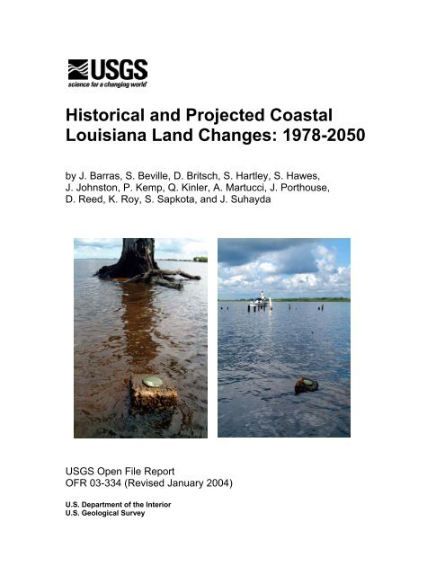
Outside front and outside back cover photographs:
Louisiana coastal landloss is dramatically depicted by these various views of USGS benchmark
“TT 62 F,” set in concrete in 1932 on dry land near the Elliot home on Bayou Couba, which is
approximately 13 miles southwest of New Orleans between Lakes Cataouatche and Salvador in
St. Charles Parish, LA. The benchmark now sits in approximately 2 feet of water, about 15 feet
from the shoreline of Couba Island. (See map below.)
Left front cover photo (dead live oak and benchmark) was taken facing north.
Right front cover photo (man fishing near pilings and benchmark) was taken facing west.
Outside back cover is a zoomed-in picture of the benchmark’s brass cap.
Benchmark legal description – Bayou Couba, near mouth of, 20 feet South, thence 5 feet West
from large lone live oak, 15 feet North from center of fireplace chimney of Mr. Elliott’s house, in
concrete post, standard tablet stamped “TT 62 F 1932”, LA south stateplane coordinates; x =
2,349,092, y = 410,266. Marker was set with a Horizontal Position ONLY.
These photos, taken in August 2003, are being used with permission © by Lane Lefort, New
Orleans, Louisiana.
Suggested citation:
Barras, J., Beville, S., Britsch, D., Hartley, S., Hawes, S., Johnston,
J., Kemp, P., Kinler, Q., Martucci, A., Porthouse, J., Reed, D.,
Roy, K., Sapkota, S., and Suhayda, J., 2003, Historical and
projected coastal Louisiana land changes: 1978-2050: USGS
Open File Report 03-334, 39 p. (Revised January 2004).
ii

Historical and Projected Coastal Louisiana
Land Changes:
1978-2050
A Report for Louisiana Coastal Area Comprehensive Coastwide
Ecosystem Restoration Study
Prepared by
John Barras 1 , Shelley Beville 2 , Del Britsch 3 , Stephen Hartley 1 ,
Suzanne Hawes 3 , James “Jimmy” Johnston 1 , Paul Kemp 4 , Quin Kinler 5 ,
Antonio Martucci 6 , Jon Porthouse 2 , Denise Reed 7 , Kevin Roy 8 ,
Sijan Sapkota 6 , and Joseph Suhayda 9
1 U.S. Geological Survey, 2 Louisiana Department of Natural Resources,
3 U.S. Army Corps of Engineers, 4 Louisiana Governor’s Office of Coastal Activities,
5 USDA Natural Resources Conservation Service, 6 Johnson Controls World Services,
7 University of New Orleans, 8 U.S. Fish and Wildlife Service, and 9 Louisiana State University
iii

Table of Contents
Page
Introduction.......................................................................................................................... 1
Data Sources.........................................................................................................................1
Data Preparation and Classification Methodology.............................................................. 2
LCA Trend Assessment Boundary............................................................................. 2
1978 Regional Habitat Data........................................................................................ 2
TM Statellite Data....................................................................................................... 2
Landsat Classification Methodology.......................................................................... 3
Coastwide 1999-2000/02 Land and Water Base Development Methodology........... 4
Recent Trends Data Set........................................................................................................ 4
Recent Trends.................................................................................................................... 11
Error Assessment............................................................................................................... 20
Classification Accuracy............................................................................................20
Positional Accuracy..................................................................................................21
Spatial GIS Analysis.................................................................................................21
Environmental and Management Factors................................................................. 22
Land Change Projection Methodology.............................................................................. 22
Previous Method of Land Loss Projections.............................................................. 23
CWPPRA Feasibility Studies.......................................................................... 23
Coast 2050....................................................................................................... 23
Davis Pond....................................................................................................... 23
Caernarvon....................................................................................................... 24
Mapping the Loss............................................................................................. 24
Land Change Calculations for the LCA....................................................................24
Step 1. Background Land-Water Change Rates........................................................25
Effect of Existing Authorized Projects..................................................................... 26
CWPPRA Project Area Background Land Change Rates and Benefits.......... 26
Davis Pond and Caernarvon Benefits.............................................................. 27
Production of Land Loss Maps for LCA.................................................................. 28
Step 2. Projected Loss-Gain Rates............................................................................ 28
Step 3. Mapping Future Loss-Gain........................................................................... 29
Limitations of Approach.................................................................................................... 31
Extreme Events......................................................................................................... 31
Assumptions on Loss-Gain Processes and Polygon Scale and Approach................ 31
CWPPRA Projects.................................................................................................... 32
Uncertainties...................................................................................................................... 33
Projected 2000 - 2050 Land Change Summary................................................................. 34
Comparisons with Previous Projections............................................................................ 35
Acknowledgments..............................................................................................................36
References.......................................................................................................................... 37
iv

Figures and Tables
Page
Tables
1 Net land loss trends by Subprovince from 1978 to 2000. 4
2 Projected net land loss trends by Subprovince from 2000 to 2050. 34
Formulas
1 Compound rate function used to calculate annual land-water change. 26
2 Compound rate function used to calculate the 50-year projected landwater
change.
28
Figures
1 1999 and 2002 data sets combined to create a 2000 Louisiana
coastwide land and water classified mosaic. 5
2 Louisiana Coastal Area (LCA) Subprovince boundaries. 6
3 Louisiana coastwide trend assessment area including the 1978 habitat
data and 1990 Landsat Thematic Mapper data. 8
4 1978 to 1990 and 1990 to 2000 spatial trend data set analysis
for southeastern Louisiana. 9
5 1978 to 1990 and 1990 to 2000 spatial trend data set analysis
for southwestern Louisiana. 10
6 1990 to 2000 spatial trend data set in the vicinity of Lake
Boudreaux and Northern Terrebonne Bay in southeastern Louisiana. 12
7 1990 to 2000 spatial trend data set in the vicinity of Bayou Perot in
southeastern Louisiana. 13
8 1990 to 2000 spatial trend data set of the Mississippi delta in
southeastern Louisiana. 14
9 1990 to 2000 spatial trend data set west of Freshwater Bayou in
southwestern Louisiana. 15
10 1990 to 2000 spatial trend data in the vicinity of Lake Grand Ecaille
in southeastern Louisiana. 16
11 1990 to 2000 spatial trend data set for southern Timbalier Bay in
southeastern Louisiana. 17
12 1990 to 2000 spatial trend data set for southwest Terrebonne in
southcentral Louisiana. 17
13 1990 to 2000 spatial trend data set for northwestern Vermilion Bay
in southcentral Louisiana. 18
14 1990 to 2000 spatial trend data set for the LaBranche Wetlands area
in southeastern Louisiana. 19
15 1990 to 2000 spatial trend data in the vicinity of Calcasieu Lake
in southwestern Louisiana. 20
16 LCA change analysis polygons. 25
17 Application of change rate in CWPPRA and LCA sites from
1978 to 2050. 27
18 Projected coastal Louisiana land changes from 2000 to 2050. 30
19 Projected coastal Louisiana land loss from 1956 to 2050. 35
v

Introduction
An important component of the Louisiana Coastal Area (LCA) Comprehensive Coastwide
Ecosystem Restoration Study is the projection of a “future condition” for the Louisiana coast
if no further restoration measures were adopted. Such a projection gives an idea of what the
future might hold without implementation of the LCA plan and provides a reference against
which various ecosystem restoration proposals can be assessed as part of the planning process.
One of the most fundamental measures of ecosystem degradation in coastal Louisiana has
been the conversion of land (mostly emergent vegetated habitat) to open water. Thus, the
projection of the future condition of the ecosystem must be based upon the determination of
future patterns of land and water.
To conduct these projections, a multidisciplinary LCA Land Change Study Group was formed
that included individuals from agencies and academia with expertise in remote sensing,
geographic information systems (GIS), ecosystem processes, and coastal land loss. Methods
were based upon those used in prior studies for Coast 2050 (Louisiana Coastal Wetlands
Conservation and Restoration Task Force [LCWCRTF] and the Wetlands Conservation and
Restoration Authority 1998, 1999) and modified as described here to incorporate an improved
understanding of coastal land loss and land gain processes with more advanced technical
capabilities. The basic approach is to use historical data to assess recent trends in land loss and
land gain and to project those changes into the future, taking into account spatial variations in
the patterns and rates of land loss and land gain. This approach is accomplished by
developing a base map, assessing and delineating areas of similar land change (polygons), and
projecting changes into the future. This report describes the methodology and compares the
current land change projection to previous projections.
Data Sources
The LCA Land Change Study Group used existing historical data derived from interpretation
of aerial photography and new data, based on classified Landsat 5 and 7 Thematic Mapper
(TM) satellite imagery, to assess current land loss and gain trends from 1978 to 2000 for
coastal Louisiana.
Data sources used in the study include:
1978 Regional Habitat Data – A coastwide raster data set based upon interpretation of
1:65,000-scale, color-infrared aerial photographs consisting of 15 land cover classes,
developed from the U.S. Fish and Wildlife Service data with a minimum resolution of 25
m, was used to assess regional habitat changes (Cahoon and Groat, 1990). The regional
habitat data set is derived from a vector data set characterizing detailed wetland habitats
by individual 7.5 minute U.S. Geological Survey’s topographic quadrangle base maps of
coastal Louisiana (Wicker, 1980). Individual habitat maps used a highly detailed coding
system developed by Cowardin and others (1979) to identify habitat types. Habitat data
coverage is based on the 1978 coastal zone boundary and does not cover the entire LCA
study area.
1990 TM Classified Data – A coastwide data set based on classified Landsat 5 Thematic
Mapper (TM) satellite data used to provide a “snapshot” of coastal land and water
1

conditions in the fall of 1990 and early spring of 1991. The data set consists of seven
Landsat TM scenes acquired between October 30, 1990 and February 24, 1991.
1999 - 2002 TM Data – A coastwide data set based on classified Landsat 7 Enhanced
Thematic Mapper Plus (ETM+) satellite data was developed to provide a “snapshot” of
coastal land and water conditions in the fall of 1999 and the early spring of 2002. The
1999 data set consists of seven Landsat ETM+ scenes acquired between October 24 and
November 27, 1999. The 2002 data set consists of seven Landsat TM scenes acquired
between January 3 and February 27, 2002.
Data Preparation and Classification Methodology
LCA Trend Assessment Boundary
The LCA trend assessment area geographically comprises the entire LCA area except for
fastlands (uplands). Those fastlands excluded from the analysis included ridges and areas
under forced drainage dominated by agriculture or human development. However, barrier
islands and other non-wetland components of the coastal ecosystem were included in the
analysis. This data set was then used as a template to extract the classified satellite data to
insure similar areas were compared for the trend assessments.
1978 Regional Habitat Data
A 1978 land-water data set was created by combining the 15 land cover classes into two
classes, land and water. The LCA trend assessment boundary was then used to extract the
1978 land-water data contained within its (study) boundaries to create a 1978 LCA landwater
data set.
TM Satellite Data
The Landsat 5 and Landsat 7 satellites are earth-observing instruments designed for land
surface monitoring and change detection and are jointly operated by the National
Aeronautics and Space Administration (NASA), the National Oceanic and Atmospheric
Administration (NOAA), and the U.S. Geological Survey (USGS). The satellite captures
images of the same location on the Earth’s surface every 16 days at approximately the
same local (Central) time, 9:30 am for coastal Louisiana. Each scene covers
approximately 185 km by 180 km and has a minimum ground resolution of 30 m. All
Landsat TM imagery used in the LCA study was resampled to 25 m to match the 25 m
spatial resolution of the historical data sets. Adjoining scenes acquired along a path are
captured within a few seconds of each other. Adjacent scenes to the east and west of the
current path are acquired every 16 days. Each scene has an overlap of approximately 18
km and a sidelap of approximately 40 km. Seven scenes are required to provide complete
coverage of coastal Louisiana. A scene contains eight bands of imagery, each recording a
discrete portion of the electromagnetic spectrum (visible to panchromatic). Each band
stores data in an 8-bit format, breaking the recorded spectral data into 256 discrete levels.
More information on the Landsat program is found at http://landsat7.usgs.gov/index.php.
The Landsat TM satellite data were classified using a standardized methodology
2

developed to allow quick and accurate classification of existing land and water conditions
at the time of image acquisition within Louisiana’s coastal wetland areas. The
methodology is not designed for developing detailed land cover information from Landsat
imagery and is based on edge enhancing and level slicing band 5 to identify land and
water on a per scene basis. Level slicing is a technique that requires visual examination of
each discrete level of spectral data to determine whether the pixels contained within the
level should be categorized as water or land.
The LCA TM data classification methodology is a refinement of a methodology originally
developed for the Louisiana Department of Natural Resources GIS lab (Braud and
Streiffer, 1992). The classification methodology was further refined for use in trend
assessments at the USGS National Wetlands Research Center (Bourgeois and Barras,
1993; Barras and others, 1994; Bourgeois, 1994) and at Louisiana State University (Braud
and Feng, 1998). All of the TM data used in the LCA study were classified over a period
of 9 months by the same remote sensing analyst using a standard classification
methodology to insure repeatability and consistency and to minimize classification
interpretation subjectivity.
Landsat Classification Methodology
Cloud-free Landsat TM 7 scenes of coastal Louisiana were obtained to provide complete
coastal coverage during the fall or winter to minimize the presence of floating aquatic
vegetation. Multiple along-path scenes were included whenever possible to maximize
contemporaneous coastal coverage. Mosaics of same-path scenes were created to reduce
the number of individual scenes requiring classification from seven to four. The band 5
(mid-infrared) subset was extracted from the mosaics to use for the land-water
classification. Band 5 is commonly used for vegetation and soil moisture measurements
and provides good land-water discrimination in Louisiana’s coastal wetlands because of
the high absorption of the mid-infrared portion of the spectrum by water and its high
reflectance by vegetation (Braud and Feng, 1998). The individual band 5 reflectance
values were compared for each mosaic to identify the water-land break in each band 5
subset. The individual band 5 reflectance values were recoded to create an initial land and
water file for each mosaic. These reflectance values were then aggregated into component
land and water classes based on the identified water-land break. A slight edge
enhancement filter (Braud and Feng, 1998) was then run to increase the contrast between
land and water values and to enhance shoreline discrimination. The water-land break was
then identified and classified for each edge-enhanced image to identify component land
and water classes. Classification, identification, and delineation of submerged and
floating aquatic vegetation and exposed flats (mud flats and sand bars) were conducted to
more accurately distinguish the water class. Each classified map was combined and
overlaid to create a composite land and water data map. The individual files were filtered
for smoothness by removing noise (unclear and erroneous pixels), and classified
contiguous coastwide land and water (CWLW) data sets for 1990, 1999, and 2002 were
created.
3

Coastwide 1999–2000/02 Land and Water Base Development Methodology
Visual examination of draft trend maps used to compare the 1990 to 1999 and 2002
CWLW data sets revealed that water levels differed in selected areas on the data sets
because of meteorological effects and management practices. The 1999 data for the
central Deltaic Plain were acquired on November 18, 1999 after mild frontal (cold)
conditions. The 2002 imagery for the same area was acquired on February 27, 2002 after
severe frontal (cold) conditions. The net effect was to lower water levels in the estuarine
marshes of the central Deltaic Plain. The interior fresh marshes actually contained more
open water in the 2002 imagery than in the 1999 imagery because of the late winter
acquisition date of 2002 imagery, when the extent of aquatic vegetation is minimal. In
the 2002 data, the area from Cote Blanche Bay west to Grand Lake contained large burns
and some surface water caused by management practices. These effects were not as
pronounced in the 1999 data. A decision was made to combine the 1999 and 2002 data
sets to create a 2000 coastwide land and water classified mosaic (CM) to more accurately
reflect “normal” land and water conditions (fig. 1). The 2000 CM served as the present
land-water base data for the historical land loss-gain assessments.
Recent Trends Data Set
All recent trend assessments include the 1990 and 2000 CM data for the LCA trend
assessment area. The 1978 to 1990 trend assessments were based on existing rates described
in Barras and others (1994). Area statistics were generated for the 1990 and 2000 CM data
and were then used to calculate the net loss rates during these periods (table 1). The LCA
study area was divided into four Subprovinces (fig. 2) for analyzing without conditions.
Table 1. Net land loss trends by Subprovince from 1978 to 2000.
1978 - 1990
Net loss
sq mi *
1990 - 2000
Net loss
sq mi
1978 - 2000
Cumulative loss
sq mi
Annual
loss
sq mi/yr
% Total loss
by area
Subprovince 1 52 48 100 4.5 15.2%
Subprovince 2 148 65 213 9.7 32.4%
Subprovince 3 134 72 206 9.4 31.3%
Subprovince 4 85 54 139 6.3 21.1%
Total sq mi 419 239 658 29.9 100%
(sq km) (1,085) (619) (1,704) (77.4)
*1978-1990 Net loss figures were based on Barras and others (1994). The 1978 to 1990 basin level and
coastwide trends used in this study were aggregated to reflect LCA Subprovinces for comparison with
the 1990-2000 data. The basin boundaries used in Barras and others (1994) were based on older
CWPPRA planning boundaries and are not directly comparable to the LCA boundary used to summarize
the 1990 to 2000 trend data. The 1990 to 2000 net loss figures include actively managed lands for
comparison purposes with the 1978 to 1990 data.
4

5
Figure 1. 1999 and 2002 data sets combined to create a 2000 Louisiana coastwide land and water classified mosaic.

6
Figure 2. Louisiana Coastal Area (LCA) Subprovince boundaries.

The 1978 habitat data covered all of the LCA area with the exception of the upper
portions of the Barataria and Terrebonne Basins and the western portion of the
Pontchartrain Basin. Loss and gain trend rates for these missing areas were assessed
by visually examining historical aerial color infared photography (1978) and USGS
topographic maps (from 1960s and 1970s). The estimated loss rates observed were so
low that we decided to use 1990 TM data to fill in the gaps of the 1978 data set (fig.
3).
Spatial changes were assessed by comparing and combining the 1978, 1990, and 2000
CM data sets to form a composite 1978 to 1990 to 2000 spatial trend data set that
identified areas of no change and areas that converted to either water or land during
the 22 year interval. The data set was then filtered to remove small areas of new
water and new land caused by a spatial misregistration between the data sets (figs. 4
and 5).
7

8
Figure 3. Louisiana coastwide trend assessment area including the 1978 habitat data and 1990 Landsat Thematic Mapper data.

9
Figure 4. 1978 to 1990 and 1990 to 2000 spatial trend data set analysis
for southeastern Louisiana.

10
Figure 5. 1978 to 1990 and 1990 to 2000 spatial trend data set analysis
for southwestern Louisiana.

Recent Trends
Wetland loss and shoreline erosion continues across much of the Louisiana coast. The
trend in the 1956-1978 period was the conversion of numerous large marsh areas (>
1,000 ha) to open water. This trend continued at a lower rate in the 1978-1990 period,
and further decreased in the 1990-2000 period (figs. 4 and 5). Shoreline erosion and the
creation of smaller interior marsh ponding continued as the primary patterns of land loss
during the last decade. Interior ponds ranged in size from 1-50 ha (about 2-125 acres),
with the majority of ponds occurring within the coastal fresh marshes. Detectable
shoreline erosion in larger lakes, bays, and ponds ranged from 50 to 300 m (164-984 ft).
The minimum detectable spatial resolution of TM multispectral imagery is 30 m.
Therefore, to accurately detect shoreline erosion by using TM imagery, the erosion must
be in excess of 50 to 60 m between the two dates at which the images are acquired. Lake
Boudreaux in Terrebonne Parish (fig. 6) and Bayou Perot in Lafourche Parish (fig. 7)
may have experienced shoreline erosion rates ranging as high as 15 to 25 m/yr (about 50-
80 ft/yr) in the last decade. During the same period, the eastern shoreline of the active
Mississippi River Delta exhibited shoreline erosion in excess of 500 m (1,640 ft) in
several locations (fig. 8) while the Gulf of Mexico shoreline, south of Rockefeller
Wildlife Refuge, exhibited 150 to 200 m (about 500-650 ft) of erosion (fig. 9).
In the Pontchartrain and Breton Sound Basins (fig. 4), some new interior ponds have
developed, and loss around the edges of large lakes and bays is widespread. In lower
Plaquemines Parish, in the vicinity of Lake Grand Ecaille the extensive loss of previous
decades has continued with the exception of areas where there are almost no wetlands left
to lose (fig. 10). In the Barataria and Terrebonne Basins (figs. 6, 10, and 11) land loss
continues in areas that were already severely affected. Interior ponding predominates in
the fresh floatant marshes, and the remnant effects of Hurricane Andrew in 1992 are
indicated by sheared ponds within the floatant areas of southwest Terrebonne (fig. 12).
Some small areas of gain are likely due to shifting of floatant mats. Fringing shoreline
erosion predominates in the estuarine marshes, although some small areas of gain are
apparent because of water level variations between the 1990 and 2000 data sets. Farther
west, from west of Atchafalaya Bay to Vermilion Bay (fig. 5), shoreline erosion
predominates, although some interior loss due to ponding is present. Land gain from
small interior ponds is related to low water conditions around West Cote Blanche and
Vermilion Bays (fig. 13).
In the Chenier Plain (fig. 5), breakup of previously intact interior marshes is apparent in
many areas. Shoreline erosion is present around the larger lakes. The Gulf of Mexico
shoreline experienced significant loss, with the exception of some gains just to the west
of Freshwater Bayou (fig. 9). Examination of multiple dates of satellite imagery for
many areas reveals varying landscapes ranging from dense marsh to open water,
depending on image acquisition time.
11

Figure 6. 1990 to 2000 spatial trend data set in the vicinity of Lake Boudreaux and
Northern Terrebonne Bay in southeastern Louisiana.
12

Figure 7. 1990 to 2000 spatial trend data set in the vicinity of Bayou Perot in southeastern Louisiana.
13

Figure 8. 1990 to 2000 spatial trend data set of the Mississippi River Delta in southeastern Louisiana.
14

Figure 9. 1990 to 2000 spatial trend data set west of Freshwater Bayou in southwestern Louisiana.
15

Figure 10. 1990 to 2000 spatial trend data in the vicinity of Lake Grand Ecaille in southeastern Louisiana.
16

Figure 11. 1990 to 2000 spatial trend data set for southern Timbalier Bay in southeastern Louisiana.
Figure 12. 1990 to 2000 spatial trend data set for southwest Terrebonne in southcentral Louisiana.
17

Figure 13. 1990 to 2000 spatial trend data set for northwestern Vermilion Bay in southcentral Louisiana.
Images of the entire coast show that movement of coastal sand bodies around the barrier islands
continues with fragmentation in areas where restoration has not occurred. A complex pattern of
erosion and land building at the Gulf of Mexico shore can be seen from Marsh Island to Sabine
Pass (fig. 5) because of mudflat accretion from the Atchafalaya and the effects of jetteries and
other coastal structures on sediment transport pathways.
The outlines of many restoration and marsh creation projects are readily apparent in the data as
areas of land gain, such as in the Labranche wetlands (fig. 14), on west of Grand Terre Island
(fig. 10), the Isles Dernieres, and with beneficial use projects near Southwest Pass (fig. 8), and
in the Sabine National Wildlife Refuge adjacent to West Cove (fig. 15). Gains are also apparent
from beneficial use of dredged material projects and from crevasse splay projects in the active
Mississippi River Delta along Southwest Pass (fig. 8). However, at the coastwide scale, the main
areas of land gain are associated with the Atchafalaya and Wax Lake Outlet deltas (fig. 12)
where delta building processes continue.
18

Figure 14. 1990 to 2000 spatial trend data set for the Labranche wetlands area in southeastern Louisiana.
19

Figure 15. 1990 to 2000 spatial trend data set in the vicinity of Calcasieu Lake in southwestern Louisiana.
Because of the scale of the available images, several years of shoreline erosion and internal
marsh degradation may occur before the loss is detectable by using Landsat TM based trend
analysis. However, visual examination of multiple dates of TM imagery using remote sensing
software clearly shows the slow degradation of wetlands. Small islands disappear and ponds
increase in size or coalesce to become larger ponds. Any such small gains experienced between
1990 and 2000 cannot be considered in this analysis but are unlikely to alter the trends and
patterns identified here.
Error Assessment
Classification Accuracy
Classification accuracy assessments were performed on the 1999 and 2002 Landsat TM imagery
to quantify the reliability of the data sets. The accuracy assessments were performed by an
experienced image interpreter who was not involved in the classification of the source TM
imagery. A stratified random sampling approach was used to create an equal number of
sampling points for the land and water classes merging each data set to provide overall accuracy.
20

To meet sampling criteria for assigning a 95% confidence level to the accuracy assessment
(Thomas and Alcock, 1984), 300 sample points (150 land samples and 150 water samples) were
collected. The overall classification accuracy was 92.0% for the 1999 data set and 92.3% for the
2002 data set. Most of the incorrectly classified samples were identified as either edge samples
located at the boundary of the land and water classes or samples comprising thin canals and
streams that were smaller than the minimum spatial resolution of the imagery.
The classification accuracy reflects how well the land and water classes were identified from the
source imagery. The accuracy assessment neither accounts for variations in land and water area
caused by meteorological conditions, tides, water management practices nor for inability to
accurately identify floating aquatic vegetation with respect to seasonal effects.
Positional Accuracy
Landsat TM imagery is designed for regional assessments and does not serve as a surrogate for
either high-resolution aerial photography or satellite imagery with spatial resolutions of 2 to 10
m. The positional accuracy of rectified TM imagery meets national map accuracy standards at
1:24,000 to 1:100,000 scales, but the level of visual detail that can be assessed from multispectral
TM imagery is limited by the 30 m spatial resolution and is best suited for scales of 1:50,000 and
smaller (Welch and others, 1985). Narrow linear features such as streams, canals, pipelines, and
ponds that are below 30 m in width may or may not be visible in the TM imagery. Even if
visible, these linear features may not be easily classified by using automated classification
techniques because mixing of pixel reflectance values between land and water.
Spatial GIS Analysis
Comparing multiple dates of Landsat scenes by using GIS spatial overlay analysis to create land
and water trend data sets requires precise spatial registration between scenes. Each classified
pixel in the source land and water data sets is compared on a pixel-by-pixel basis. A resultant
spatial trend data set is created identifying the changes among the source land and water data
sets. A change pixel can be classified as: (1) land to land - no change, (2) water to water - no
change, (3) land to water - change (loss), or (4) water to land - change (gain). The pixels in both
data sets should occupy the same location or the resultant trend data set will exhibit false land
losses and gains that are due to misregistration (+/- 1 pixel). These positional shifts are generally
uniform in nature and appear as thin strips of loss or gain bordering the shorelines of canals and
ponds. Spatially comparing two georegistered mosaicked coastwide data sets, such as the 1990
and the 2000 CM data sets for Louisiana’s complex coastal area, may result in a positional error
of as much as 30 m because of misregistration. The original trend data sets resulting from
overlay analysis almost always require some type of filtering to reduce false trend “noise” caused
by slight positional errors and to isolate real trends between the source data sets.
The net loss calculations derived by comparing total land and water areas between the coastwide
data sets eliminate the false noise inherent in GIS trend data, but they do not indicate where
trends are occurring within the coastal area. Net trends based on simple area calculations are
apparent; a land and water data set has either more land or more water. However, very complex
changes may be reflected in the spatial data that cannot be determined from simple area
21

calculations denoting land or water areas. The spatial trend data depict and quantify changes in
land and water areas. Accurately interpreting and quantifying these changes requires
acknowledgment that some degree of procedural error is inherent within the trend data.
Environmental and Management Factors
The errors in quantifying temporal land and water change in the Louisiana coastal wetlands using
classified imagery are also associated with low water conditions and management-induced
changes. The Landsat TM satellite records a digital picture of a discrete instant in time for a 180
km x 185 km section of the coast. Snapshots at different time intervals are compared to
determine trends in land loss and gain for a specific time period assuming that differences caused
by environmental and management conditions during image acquisition are negligible. Known
factors affecting trend estimates include (1) meteorological and tidal conditions at the time of
image acquisition, (2) coastal morphology, (3) vegetative vigor, (4) seasonality, (5) presence or
absence of floating aquatic vegetation, (6) water management practices, particularly within the
Chenier Plain (LCWCRTF, 2002), (7) prevalence of burned marsh, and (8) impacts from
infrequent catastrophic events such as hurricanes and floods (Bourgeois, 1994). Analysis of
Landsat TM scene acquired on October 16, 2002, after the central Louisiana coast was struck by
Hurricane Lili on October 3, 2002, revealed creation of over 256.6 ha of new ponds in a formerly
dense healthy marsh that had shown no significant loss since the late 1970s (Barras, 2003).
All these factors contribute to error in assessing trends in land loss or gain rates. These errors
associated with landscape conditions (environmental and management operations) limit the use
of single values to describe trends in land loss, but require the use of a range in values that
capture many contributing factors. There are not enough current classified Landsat TM data
points available to accurately assign an error range to current trend data. Conservative estimates,
based on knowledge gained during the LCA trend assessment and the classified land and water
data set error assessment, place the trend error range at +/- 25% for this analysis. The same
factors will also affect trend interpretation based on higher spatial resolution data from
photography and satellites. The higher spatial resolution will allow a more precise location of
the land and water interface, to within a few meters rather than 25 m, but the classification of that
interface will still be affected by environmental and management conditions prevalent during
image acquisition.
Land Change Projection Methodology
The future of the Louisiana coastal landscape has been projected in many ways since the land
loss issue was recognized. The methods used have varied from province-scale extrapolation of
land loss trends (Gagliano and others, 1981) to projection of shoreline position decades into the
future (Gagliano, 1994). Recent improvement in GIS technology and refining methodology have
allowed the LCA study to develop and build better projection based on previous efforts.
22

Previous Method of Land Loss Projections
CWPPRA Feasibility Studies
In 1995, at the inception of the two Coastal Wetlands Planning, Protection and Restoration
Act (CWPPRA) feasibility studies (Mississippi River Sediment, Nutrient, and Freshwater
Diversion Reanalysis and Barrier Shoreline), the U.S. Army Corps of Engineers determined
that the land loss projection methodology in both studies should be consistent. A
multiagency group of marsh experts was convened in 1995. This group determined that the
1974 to 1990 land loss analysis (early results from Britsch and Dunbar, 1993) was the best
estimate of future loss. The 1974 to 1983 loss rate was higher than the most recent period of
1983 to 1990. The group concluded that using a rate over a longer time period (1974 to
1990) would provide a better account for the sea level-subsidence factor. The group drew
polygons around areas where causes of land loss seemed to be similar. The annual
percentage of marsh loss between 1974 and 1990 was determined for each polygon. These
annual percentages were used to project future land-water trends in the two CWPPRA
feasibility studies (see http://www.lacoast.gov for more information).
Coast 2050
The interagency Coast 2050 Loss Projection Team was formed in 1997. The results of their
work are in the Coast 2050 Plan (LCWCRTF, 1998). This team concurred with the 1995
CWPPRA group that the 1974 to 1990 loss rate was the best with which to project future
loss. They drew new, smaller polygons that more accurately projected loss patterns and
excluded uplands. This team made adjustments in the projected loss to account for benefits
of CWPPRA projects and the Davis Pond and Caernarvon Diversions, described below.
Davis Pond
The 1984 Louisiana Coastal Area Final Environmental Impact Statement (FEIS, 1984),
which covered the Davis Pond (fig. 14) and Caernarvon Freshwater Diversions, projected
that 50% of the land loss in the receiving area would be prevented by the project. However,
the “future without” land loss rates projected to occur at the time of the FEIS were much
higher and less refined than those based on more current data sets. The Coast 2050 Loss
Projection Team used the 1974 to 1990 loss rates as described above. In addition the team
corrected acreages of wetland types and subtracted human-caused loss. This analysis group
also incorporated information from LSU Natural Systems Laboratory hydrodynamic model
runs that indicated where water from Davis Pond would flow. These simulations provide
insights as to the spatial distribution of where land loss may be prevented. In order to
determine the location of benefits (land preserved or created) to be added, the data from this
analysis were used in conjunction with the Coast 2050 mapping units. The net effects of the
Davis Pond project incorporated into the Coast 2050 future projection are 29,500 acres
(11,938 ha) preserved and 3,500 acres (1,416 ha) created over the 50-year project life span.
23

Caernarvon
Using the same protocol as the Davis Pond analysis, the projected land loss reduction was
allocated to the appropriate Coast 2050 mapping units. The net effects of the Caernarvon
project incorporated into the Coast 2050 future projection are 26,100 acres (10,562 ha)
preserved or created over the 50-year project life span.
Mapping the Loss
The Coast 2050 Loss Projection Team used the 1993 Landsat image to determine where
within each polygon the loss might be located. The team selectively modified parts of the
Landsat image, based on the brightness values, to best estimate the net acreage of marsh lost
in each polygon by 2050. Each 25-m pixel on the image contained brightness values based
on combining bands from the original Landsat data. Brightness was then used as the landwater
boundary criteria. Areas with brightness higher than the criterion were predicted to be
land in 2050, and those with lower brightness were predicted to be water in 2050.
To depict land loss on the image, the brightness criterion for land was adjusted to a higher
value, which resulted in less land being depicted on the image. This adjustment was made
iteratively until the amount of land in each polygon matched the acreage projected to remain
in that polygon in 2050. Reducing the brightness criterion removed land from the image.
The amount of land preserved by CWPPRA projects (based on their Wetland Value
Assessment [WVA]) (Environmental Work Group, 1998) and the river diversions was then
added to the respective image in each polygon.
This technique assumes that the areas of lower brightness on the image are areas of transition
from land to water and that these areas will be lost preferentially over areas with higher
brightness. This assumption thus projects spatial patterns of land loss based upon the
existing balance of land and water, as reflected in the brightness of the image. Similarly,
land building is also deemed to occur in the water areas with brightness values closest to
those of land.
Land Change Calculations for the LCA
The sources of imagery (1978 habitat data, 1990 TM data, and 1999-2002 TM data) were used to
derive recent land change rates that, in turn, were used to project future change (land-water
conversion) rates and patterns. Similar to the previous method, the LCA Land Change Study
Group created polygons around areas with similar loss-gain patterns. The annual percentage of
land loss between 1978 and 2000, or between 1990 and 2000 where 1978 data were not
available, was determined for each polygon. Those annual percentage rates were used to project
future trends in land-water changes. Adjustments to future projections for Caernarvon, Davis
Pond, and CWPPRA projects were based on the methods of the previous analysis.
24

Step 1. Background Land-Water Change Rates
The LCA Land Change Study Group delineated polygons (fig. 16) across the coastal zone
through visual examination of land-to-water or water-to-land (land-water) changes during the
period of 1978 to 2000. These polygons were delineated based on geography, extent of landwater
change, pattern of change, suspected cause of change, and expertise and experience of
the Land Change Study Group. In total, 183 polygons (fig. 16) were delineated by this
analysis. By delineating areas of similar change rates and patterns, a geographic-specific
change rate could be applied to each polygon to project future land-water change. The
methodology used to calculate the recent historical or “background” land-water change rate
for each LCA polygon was based on classified Landsat TM imagery from the following
years:
Majority of LCA (study area) coast: 1978 to 2000. (Represents the most applicable data
sets for determining a change rate for recent history.)
Portion of LCA (study area) coast where 1978 data were not available: 1990 to 2000
(Viewed to represent most applicable data sets for determining a change rate for recent
history where 1978 data were not available.)
Majority of CWPPRA project areas: 1978 to 1990 (Some CWPPRA projects produced
an immediate and one-time increase in land between 1990 and 2000; to project such land
increases into the future was not considered to be appropriate. The acreage created or
predicted to be created by CWPPRA projects was factored into the analysis as described
below.)
Figure 16. LCA Change Analysis Polygons.
25

Small portion of CWPPRA project areas where 1978 data were not available: 1990 to
2000. (Fortunately, none of the CWPPRA projects in this area produced the immediate
and one-time increases in land referenced above.)
The compound rate function (formula 1) was used to calculate the annual land-water change
rate. Change rates (land-water conversion) were not calculated for actively managed areas.
These areas were masked out for each of the data sources because active water management
can produce misclassification of land versus water. For example, when an area is
intentionally flooded for management purposes, the area would likely be classified as water,
potentially showing up as land loss when a true loss did not actually occur. (Note: These
areas were excluded from the source data so they would not be used in generating the change
rates.) Actively managed areas were depicted as they appeared in the 2000 source with no
change in the 50-year projection.
Formula 1. Compound rate function used to calculate the annual land-water change.
Number of years = 22, except for 1990 data source where number of years = 10.
r = rate of annual land-water change.
IF (water2000 - water19(78 or 90) = 0) then no net change
r = 0
IF (water2000 - water19(78 or 90) < 0) then net land gain
⎛
⎜⎛
water2000
⎞
r = ⎜⎜
⎟
⎜⎝
water19(
78or90)
⎠
⎝
1
# ofYears
⎞
⎟
⎟ −1
⎟
⎠
OR if (water2000 - water19(78 or 90) > 0) then net land loss
⎛
⎜⎛
land 2000 ⎞
r = ⎜⎜
⎟
⎜⎝
land19(
78or90)
⎠
⎝
1
# ofYears
Effect of Existing Authorized Projects
⎞
⎟
⎟ −1
⎟
⎠
CWPPRA Project Area Background Land Change Rates and Benefits
Except as noted above, land change within CWPPRA project areas was based on 1978
and 1990 classified Landsat imagery. The benefits of CWPPRA projects (funded-forconstruction
as of October 2002) are accounted for in the 50-year projection in the
following manner. Small polygons that reflect the CWPPRA project area were drawn
26

Acreage
within the larger LCA polygons. The projected net land acreage gain of the CWPPRA
project at the end of 20 years, based on WVA, was then added to the polygon in the year
2020.
The land acreage was added at year 20 because that is the standard life of CWPPRA
projects, and addition at this point assumes that all funded-for-construction CWPPRA
projects were built in 2000. Each CWPPRA polygon was adjusted for the first 20 years
to include either the 1978 to 1990 or 1990 to 2000 change rates (background change
rate). Because of the 20-year life for CWPPRA projects, the background change rate is
applied to the entire polygon for the remaining 30 years of the LCA projection, for
example, years 2020 to 2050 (fig. 17). CWPPRA projects not funded for construction as
of October 2002 were not considered in this analysis. The Coastwide Nutria Control
Program was not considered in the analysis because of the lack of geographic specificity
of the predicted benefits.
500
400
(a)
(b) (c) (d)
300 (e)
CWPPRA
Addition
(f)
200
100
1978 1990 2000 2020
Year
2050
Figure 17. Application of change rate in CWPPRA and LCA sites from 1978 to 2050.
Note: (a) Estimated change rate for the1978 to 1990 time interval that was applied to all CWPPRA sites.
(b) Estimated change rate applied to the CWPPRA sites that needed the 1990 to 2000 time
interval.
(c) The change rate applied to the first 20 years of CWPPRA projects; this change rate is taken
from either (a) or (b).
(d) The change rate applied to the last 30 years of CWPPRA projects; this change rate is the same
as (c).
(e) Estimated change rate from 1978 to 2000 for all non-CWPPRA projects.
(f) The change rate applied to the LCA polygons for 50 years.
Davis Pond and Caernarvon Benefits
The benefits of the Davis Pond and Caernarvon projects are accounted for in the 50-year
projection by adding land acreage to the appropriate rate change polygon(s) at year 50 of
the projection. The land acreage is added at year 50 because that is the standard life of
Water Resources Development Act (WRDA) projects, and this assumes that those
projects were built in 2000. The land acreage added at year 50 is the projected 50-year
27

net acreage for each project as determined through the above-described project-specific
projections.
Production of Land Loss Maps for LCA
The 2000 Landsat image was used to determine the location of land loss within each polygon.
Similar to the previous method, brightness values were used as the land-water boundary
criterion. However, in the previous land-water trend analysis, each polygon of the Landsat
image was manually adjusted for brightness by summing the lower histogram values until the
expected land-water acreage was achieved. The new automated method uses Environmental
Systems Research Institute’s (ESRI) ArcView Avenue code to adjust the histogram threshold.
This new threshold was then applied to the Landsat image to make the image lose or gain land
based on the change rate criteria.
Step 2. Projected Loss-Gain Rates
The 50-year projected land-water change for each LCA polygon is calculated
based on the compound rate function (formula 2). A grid (cell) for each LCA and
CWPPRA polygon with actively managed areas masked out was created from the 2002 TM
image (band 5).
Formula 2. Compound rate function used to calculate the 50-year projected land-water change.
Number of years = 50, except for CWPPRA sites
IF (water2000 - water19(78 or 90) < 0) then net land gain
years
( )
( land2000
+ water2000)
− land 2000*
( Rate)
( land2000
+ water2000)
2050
water 2050 = 1+
land 2050 =
− water
OR, IF (water2000 - water19(78 or 90) > 0) then net land loss
( ) years
2000 * Rate
( land 2000 water2000)
land 2050 = land 1+
water 2050 = +
− land 2050
Band 5 of the TM image was used because it shows the most contrast in the land-water
interface. The TM data were used to find the water threshold level based on the projected
loss or gain. Assuming that low reflectance values on the TM scene equate to water, the
water threshold is achieved by summing the low end values of the histogram until the
projected value is reached. For example, with a projected land loss of 100 acres (40.5 ha), the
threshold would be set to 2 as seen in the following histogram.
28

Threshold Histogram Values Acreage Sum
... ... ... ...
3 1000 154.44 317.09
2 500 77.72 162.65
1 450 69.49 84.93
0 100 15.44 15.44
Acreage was calculated by multiplying the histogram value by 25 x 25 x 0.0002471054. The
25 m value represents the resolution of the TM imagery used (25 is the meter size of each
raster pixel, multiplied together to get square meters, then multiplied by the factor
0.0002471054 to convert square meters into acres). Once threshold values have been
determined each TM grid histogram is reclassified. In this example, threshold 0 and 1 would
be predicted to be water in 2050 and threshold 2 and above would be predicted as land.
Step 3. Mapping Future Loss-Gain
All reclassified LCA and CWPPRA grids along with the actively managed areas were
merged back together into the final 50-year projected grid. The final grid and the classified
2000 imagery were then used in a land-change analysis to determine the final land loss and
gain (fig. 18). The assessment of the methodological error shows that the projected acreages
of the modified Landsat imagery are within 3% of the calculated numbers of land change.
29

30
Figure 18. Projected coastal Louisiana land changes from 2000 to 2050.

Limitations of Approach
Extreme Events
This projection methodology assumes that the events and processes contributing to land
loss or gain within the polygons from 1978 to 2000 continue into the future. Therefore, it
includes the effects of extreme events only if they occurred during the period 1978 to
2000. The method is not truly probabilistic as it uses the actual occurrence rather than the
average return period of the events that affected the coast during that time. The period
does include tropical storms and hurricanes impacting the Louisiana coast, for example,
Hurricane Juan in 1985 and Hurricane Andrew in 1992. The effects of the events, both in
eroding shorelines and providing sediments to increase marsh elevation, are part of the
projection. Similarly, the effects of both flood and low water years on the Mississippi
River that occurred between 1978 and 2000 are projected to occur with the same
frequency and magnitude in the future. Thus, the effect of flood years (including 1983,
1993, and 1997) that likely contributed to land gain in the Atchafalaya Delta area are
included without offsetting the effects of low water years such as 1989 and 1992. The
drought conditions of 1999-2001 are partially reflected in the projection. For example,
the meshing of data sets from late 1999 and early 2002 for the base years reflects the
inclusion of the effects of the drought. Given the uncertainties regarding the return
period of drought events of this magnitude, it was not possible to fully incorporate the
effects of intense drought in projecting trends on land loss or gain rates.
Assumptions on Loss-Gain Processes and Polygon Scale and Approach
A fundamental assumption of this approach to land change projections is that the
processes causing land loss and land gain will continue into the future at the same rate
and at the same spatial scale that they occurred at in the recent past. The use of 1978 to
2000 as a base period to derive the future land change rate is important as it largely
postdates a period of massive human alteration of the coastal landscape associated with
dredging of canals for oil and gas exploration and for navigation. Thus, the direct effects
of these extensive dredging activities are not reflected in the rates that are projected.
Indirect and ongoing effects of these activities that may result in land loss, such as
altering marsh hydrology or basin-scale salinity gradients, are projected to occur in the
future at the average rate that they have in the past 2 decades.
More chronic regional-scale problems such as subsidence and altered patterns of
sediment delivery from the Mississippi River are projected to have the same effects in the
future as in the past. Although recent data (Morton and others, 2002) suggest that
extensive hydrocarbon extraction from subsurface reservoirs led to localized high rates of
subsidence in previous decades, the greatest volumes of hydrocarbons were extracted in
the 1960s and 1970s, at least in the fields examined by Morton and others (2002). The
extraction likely reactivated faults leading to subsidence, but the timing of fault
movement relative to mineral extraction has yet to be clearly identified. Thus, it is
possible that during the 1980s such localized high subsidence was still occurring and
resulting in land loss. Such land loss is incorporated in the rate projected into the future.
31

However, the spatially explicit projection methodology means that rates of land loss (or
gain) are projected to continue only within the boundaries of individual polygons. Thus,
any high rates associated with these withdrawal effects and not expected to continue into
the future will be projected only within individual polygons.
Where small, very localized areas of high loss (or gain) occur within otherwise relatively
stable areas of the coast, it is frequently not possible to identify them as separate
polygons for projection. In these cases, the rate of the entire polygon will include both the
locally high rate and the average rate, which will be projected across the whole area.
Thus, the projected loss may not occur in the immediate vicinity of the past loss but will
be distributed across the polygon. This is an artifact of the spatial scale at which the
methodology allows us to project land loss. The goal of the method is to provide a
spatially explicit projection. However, it cannot project in detail all the complex patterns
of coastal land loss and gain occurring across the coast.
CWPPRA Projects
The attempt to incorporate the benefits of funded-for-construction (as of October 2002)
CWPPRA projects relied on assumptions that produced some accompanying limitations.
All funded-for-construction CWPPRA projects were assumed to be constructed in 2000.
However, some land creation projects were built prior to 2000, hence their net land
acreage is “double counted,” first in the 2000 data base and then again at year 20 of the
projection. This “double counting” is estimated at 4,500 acres (1,821 ha), and could
result in a slight overestimate of land acreage at the end of the 50-year projection.
Furthermore, not all funded-for-construction CWPPRA projects were constructed by
2000 and some may not ever be constructed. Therefore, their estimated net land acreage
may be added in sooner than actually realized, if ever realized, and could result in a slight
over projection of land acreage at the end of the 50-year projection. A second
assumption is that all funded-for-construction CWPPRA projects will achieve 100% of
their estimated net land acreage at the end of 20 years. However, some CWPPRA
projects may have been slightly reduced in scope during the design phase without a
reevaluation of benefits and not all projects perform as well as predicted. Either of these
situations could result in a slight overestimate of land acreage at the end of the 50-year
projection. Another assumption states that for all funded-for-construction CWPPRA
projects, the project area will resume a “background” change rate after 20 years, but some
CWPPRA projects can be expected to produce benefits beyond year 20. Resuming the
“background” change rate could result in a slight underestimate of land acreage at the end
of the 50-year projection. In addition, the Coastwide Nutria Control Program has
received some implementation funding; however, it was not considered in the analysis
because of the lack of geographic specificity of predicted benefits and the present level of
funding being limited to 5 years. Should the project accomplish its estimated benefits
(about 15,000 net acres [6,070 ha] of land at the end of 20 years), the coastwide
projection of land acreage could be slightly underprojected.
32

Uncertainties
This projection method can only incorporate the effects of events that occurred in the
past. Therefore, the effects of future changes in climate and climate variability are not
directly incorporated into the projection. The effects of potentially important factors such
as sea-level rise are assumed to continue at the same rate that they have in the past. This
assumption may not be as problematic as it might appear. Louisiana coastal wetlands
have been subjected to high rates of relative sea-level rise for centuries, which is due, in
part, to high subsidence rates associated with the compaction and dewatering of deltaic
sediments. The effect of historical subsidence and relative sea-level rise over the last 2
decades is incorporated into the projection. Some Louisiana marshes have adjusted to
these high rates, in some cases over 1 cm/yr, while others are experiencing stress which
may in part be driven by the relative sea-level rise. Morris and others (2002) recently
predicted that in areas of high sediment loading, such as those in Louisiana, the limiting
rate of relative sea-level rise for salt marshes is, at most, 1.2 cm/yr. Future increases in
eustatic sea-level are projected to be approximately 20 cm by the year 2050 (Field and
others, 2001). While many Louisiana marshes may currently be at their saturation limit,
with respect to the relative sea-level rise scenario they may further deteriorate remarkably
under future sea-level rise conditions. Morris and others (2002) considered tidal flooding
to be the primary determinant of sediment deposition rather than the episodic high water
events associated with frontal passages, tropical storms, and hurricanes. These factors
likely contribute to the sustainability of existing Louisiana marshes, and it is not known
how marshes will accommodate future increases in relative sea-level rise. Thus, although
these projections do not take future increased sea-level rise into account, there is
sufficient uncertainty regarding how Louisiana marshes might respond to these increases
making their inclusion in the projection challenging.
In addition to sea-level rise, future changes in climate will influence the quantity and
timing of freshwater delivery to coastal estuaries. Future changes in the flow regime of
the Mississippi River are important considerations for the design and operation of river
diversions to restore the coast of Louisiana. However, the existing diversions,
Caernarvon and Davis Pond, divert a very small amount of current river discharge.
Therefore their operation will likely only be minimally affected by climate change. In
Subprovince 3, the effect of the Atchafalaya River, in both delta building and
rejuvenation of adjacent wetlands, is considered in this projection to proceed at the same
rate as in the last several decades. As the effect of climate change on runoff in the
Mississippi Basin, and therefore the Atchafalaya, ranges from increasing discharge to
decreasing discharge depending on the model used (Scavia and others, 2002), it is
difficult to assess how such changes could influence the land building processes
important in Subprovince 3. Whatever the net effect of climate change on basin runoff,
most climate projections agree that precipitation regimes in the future will be
characterized by more frequent high-intensity rainfall events and that runoff regimes will
therefore become more intense. In most drainages, these “flashfloods” will most likely
produce increased sediment runoff, depending on concomitant changes in land cover
conditions. Thus, for the coastal zone, while there is uncertainty regarding the future
discharge and sediment delivery regimes on an annual basis, the future conditions may
33

include periodically increased sediment delivery. With higher or lower river discharge,
greater relative sediment delivery will support land building and wetland rejuvenation in
the area influenced by the Atchafalaya River. As with sea-level rise, the exact changes
that will occur on the coast associated with future climate change have not been explicitly
included in this projection. These exact changes cannot be estimated until there is
increased understanding of the climate change scenarios and landscape response.
However, as shown in this discussion, some aspects of coastal dynamics may not be as
sensitive to conditions associated with climate change as they are to the many human
modifications to the coast that have resulted in the degradation of the system.
Projected 2000-2050 Land Change Summary
The projected 2000-2050 land changes, based on the analysis described above, project
total land loss as 674 sq mi (1,746 sq km) and total land gain as 161 sq mi (417 sq km).
These gains were from the following sources: CWPPRA projects, 54 sq mi (140 sq km);
Caernarvon diversion, 25 sq mi (65 sq km); Davis Pond diversion, 53 sq mi (137 sq km);
Atchafalaya Delta building, 14 sq mi (36 sq km); and Mississippi River Delta building,
15 sq mi (39 sq km). Thus, the projected net land loss is 513 sq mi (1,329 sq km) (table
2). Land loss curves depicting land loss from 1956-2050 project gross loss (without
projected gain) at 2,199 sq mi (5,695 sq km) and net loss (with projected gains) at 2,038
sq mi (5,278 sq km) (fig. 19).
Table 2. Projected net land loss trends by Subprovince from 2000 to 2050.
Land in
2000
sq mi
Land in
2050
sq mi
Net
Land loss
sq mi
% Land loss
between 2050
and 2000
Land loss
sq mi/yr
% Total loss
by area
Subprovince 1 1,331 1,270 61 4.61% 1.23 12%
Subprovince 2 1,114 928 186 16.68% 3.71 36%
Subprovince 3 1,975 1,746 229 11.59% 4.58 45%
Subprovince 4 1,431 1,394 37 2.59% 0.74 7%
Total sq mi
(sq km)
5,851
(15,154)
5,338
(13,825)
513
(1,329)
8.77% 10.26
(26.57)
Note that total percentage of land loss is the percentage of total net land loss (513 sq mi)
in 2050 to the existing land (5,851 sq mi) in 2000.
34
100%

Figure 19. Projected coastal Louisiana land loss from 1956 to 2050.
Note: With the projected gain, the net loss from year 1956 to 2050 is estimated to be 2,038 sq
mi (5,278 sq km) whereas without the projected gain, the estimated total loss amounts to
2,199 sq mi (5,695 sq km).
Comparisons with Previous Projections
This projection of land-water conditions presented here (table 2, fig. 18) uses the same
fundamental methodology as the projection included in the Coast 2050 Plan (LCWCRTF,
1998). However, the projected magnitude of change by 2050 is the net loss of 513 sq mi
(1,329 sq km), rather than the almost 1,000 sq mi (2,590 sq km) projected in 1998. There
are several reasons for this change in projection:
- The 1998 projection was based on land loss rates between 1974 and 1990. The base
period for the current projection is 1978 to 2000 and thus the lower rates in the
1990s project lower rates into the future.
- The spatial patterns of land loss between 1974 and 1990 projected in the earlier
analysis were based on data derived from aerial imagery, and the procedure used to
develop the maps focused on land loss rather than land gain (Britsch and Dunbar,
1993). Thus, the 1974 to 1990 data encompassed only “gross loss” and did not include
any land gain occurring in the study area. The current analysis includes both loss and
gain and the net result of both processes is projected forward in a spatially explicit
manner.
- The Britsch and Dunbar (1993) data set was based on analysis of aerial photography
and was largely restricted to the nonforested areas of the coast. Little data were
35

available for the upper basins, dominated by cypress-tupelo swamps and bottomland
hardwoods. In the 1998 analysis, expert judgment was used to estimate the future loss
in these areas and resulted in an estimate of over 360 sq mi (932 sq km) of swamp loss
(out of the 1,000 sq mi [2,529 sq km]). In the current analysis, the Landsat TM
(satellite databases) used for 1990 and 2000 covered the entire area. Therefore, using
the same methodology, quantitative projections for the entire LCA area were possible.
- The loss shown in actively managed areas in the Britsch and Dunbar (1993) data was
projected in the 1998 analysis. The current projection, however, excluded these areas
because the LCA Land Change Study Group recognized that, at the time of the
imagery, their classification as either land or water reflected the prevailing
management regime rather than any trajectory of change in the coastal landscape.
The LCA Land Change Study Group considers that the net contribution of these four
factors, and other minor differences in the projection methodology, account for the
differences in the magnitude of the future loss projection. Most of these changes in the
projection procedure represent a more thorough consideration of the factors contributing
to coastal land change as a result of our increasing understanding of the coast and the use
of improved technology.
Acknowledgments
Authors of this report would like to thank Dr. Bill Good, Dan Lewelyn, and Honora
Burras of LA-DNR; Charles Demas and George Arcement of USGS-WRD; Pete
Bourgeois and Clint Padgett of USGS-BRD; and Marty Floyd of USDA-NRCS for their
reviews and comments with valuable suggestions for improvement. We express our
gratitude to Dr. Robert Twilley of the University of Louisiana at Lafayette for his
extensive and detailed review. We also thank Beth Vairin of USGS-BRD and Lana
Wiggins of Johnson Controls World Services, Inc. for editing the manuscript at various
stages.
Thanks are also extended to Dr. John Day (Louisiana State University) and Dr. Buddy
Clairain (USACE), Co-chairs, in addition to the other members, of the Louisiana Coastal
Area (LCA) National Technical Review Committee for providing comments and
suggestions during the preparation of the report. Jay Grymes (Louisiana State
Climatologist) and Gregory Steyer (Ecologist, USGS-BRD) provided ancillary
hydrologic and climatic data that were used in calculating land loss rates.
36

References
Barras, J.A., Bourgeois, P.E., and Handley, L.R., 1994, Land loss in coastal Louisiana
1956-90: National Biological Survey, National Wetlands Research Center, Open
File Report 94-01. 4 p. 10 color plates.
Barras, J.A., 2003, Changes to Cote Blanche Hydrologic Restoration (TV-04)
Area after Hurricane Lili: U.S. Geological Survey, National Wetlands Research
Center, map-id USGS-NWRC 2003-11-112. poster.
Bourgeois, P.E., 1994, Discerning broken marsh from landsat thematic mapper satellite
imagery: Baton Rouge, Louisiana State University, M.S. thesis. 148 p.
Bourgeois, P.E., and Barras, J.A., 1993, Quick and effective land/water delineation from
Landsat TM satellite imagery for the Louisiana coastal zone. 4th National U.S.
Fish and Wildlife Service GIS workshop, May 3-6, 1993, Lafayette, Louisiana.
Braud, D.H., and Streiffer, H.R., 1992, A collection of image processing and GIS
techniques and procedures designed and developed by Decision Associates, Inc.
for the Louisiana Department of Natural Resources. Internal document.
Braud, D.H., and Feng, W., 1998, Semi-automated construction of the Louisiana
coastline digital land/water boundary using landsat thematic mapper satellite
imagery. Department of Geography and Anthropology, Louisiana State
University. Louisiana Oil Spill Research and Development Program, OSRADP
Technical Report Series 97-002.
http://www.osradp.lsu.edu/1997_Deliverables/Braud97/Braud97.htm.
Britsch, L.D., and Dunbar, J.B., 1993, Land-loss rates: Louisiana coastal plain: Journal
of Coastal Research, v. 9, p. 324-338.
Cahoon, D.R. and Groat, C.G., eds., 1990, A study of marsh management practice in
coastal Louisiana, Volume II, Technical Description. Final report submitted to
Minerals Management Service, New Orleans, LA. Contract No. 14-12-0001-
30410. OCS Study/MMS 90-0075. 309 p.
Cowardin, L. M., Carter, V., Golet, F.C., and LaRoe, E.T., 1979, Classification of
wetlands and deepwater habitats of the United States. GPO 024-010-00524-6:
Washington, DC, U.S. Government Printing Office. 103 p.
Environmental Work Group, 1998, Wetland Value Assessment Methodology and
Community Models. Environmental Work Group: Coastal Wetland Planning,
Protection, and Restoration Act (CWPPRA). 13 p. plus appendix.
37

FEIS, 1984, Final Environmental Impact Statement Louisiana Coastal Area. Louisiana
Freshwater Diversion to Barataria and Brenton sound basins: U.S. Army Corps of
Engineers. 114 p.
Field, J.C., Boesch, D.F., Scavia, D, Buddemeier, R.W., Burkett, V., Cayan, D.R.,
Fogarty, M., Harwell, M.A., Howarth, R.W., Mason, C., Reed, D.J., Royer, T.C.,
Salinger, A.H., and Titus, J.G., 2001, Potential consequences of climate
variability and change on coastal areas and marine resources, chap. 16 of National
Assessment Synthesis Team ‘Climate Change Impacts on the United States: The
Potential Consequences of Climate Variability and Change.’ Report of the US
Global Change Research Program: Cambridge, UK, Cambridge University Press.
620 p.
Gagliano, S.M., Meyer-Arendt, K.J., and Wicker, K.M., 1981, Land loss in the
Mississippi River Deltaic Plain: Transactions-Gulf Coast Association of
Geological Societies, v. 31, p. 295-300.
Gagliano, S., 1994, An Environmental-Economic Blueprint for Restoring the Louisiana
Coastal Zone: The State Plan. Report of the Governor's Office of Coastal
Activities Science Advisory Panel Workshop: Baton Rouge, LA, Coastal
Environments, Inc., 52 p.
Louisiana Coastal Wetlands Conservation and Restoration Task Force and the Wetlands
Conservation and Restoration Authority (LCWCRTF), 1998, Coast 2050:
Toward a Sustainable Coastal Louisiana, The Appendices. Appendix B –
Technical Methods: Baton Rouge, LA, Louisiana Department of Natural
Resources, 169 p.
Louisiana Coastal Wetlands Conservation and Restoration Task Force and the Wetlands
Conservation and Restoration Authority (LCWCRTF), 1999, Coast 2050:
Toward a Sustainable Coastal Louisiana: Baton Rouge, LA, Louisiana
Department of Natural Resources, 161 p.
Louisiana Coastal Wetlands Conservation and Restoration Task Force
(LCWCRTF), 2002, Hydrologic Investigation of the Louisiana Chenier Plain:
Baton Rouge, LA, Louisiana Department of Natural Resources, Coastal
Restoration Division, 135 p. plus appendices.
Morris, J.T., Sundareshwar, P.V., Nietch, C.T., Kjerfve, B., and Cahoon, D.R., 2002,
Responses of coastal wetlands to rising sea level: Ecology, v. 83, no. 10, p. 2869-
2877.
Morton, R.A., Buster, N.A., and Krohn, M.D., 2002, Subsurface Controls on Historical
Subsidence Rates and Associated Wetland Loss in Southcentral Louisiana: Gulf
Coast Association of Geological Societies Transactions, v. 52, p. 767-778.
38

Scavia, D., Field, J.C., Boesch, D.F., Buddemeier, R.W., Burkett, V., Cayan, D.R.,
Fogarty, M., Harwell, M.A., Howarth, R.W., Mason, C., Reed, D.J., Royer, T.C.,
Sallenger, A.H., and Titus, J.G., 2002, Climate change impacts on U.S. coastal
marine ecosystems: Estuaries, v. 25, no. 2, p. 149-164.
Thomas, I.L. and Alcock, G.M., 1984, Determining the confidence level for a
classification: Photogrammetric Engineering and Remote Sensing, v. 50, p. 1492-
1496.
Welch, R., Jordan, T.R., and Ehlers, M., 1985, Comparative evaluations of the geodetic
accuracy and cartographic potential of Landsat-4 and Landsat-5 Thematic Mapper
image data: Photogrammetric Engineering and Remote Sensing, v. 51, p. 1799-
1812.
Wicker, K. M., 1980, The Mississippi Deltaic Plain Habitat Mapping Study. 464 maps:
U.S. Fish and Wildlife Service, Office of Biological Services. FWS/OBS –
79/07.
39