Wah Chiu wah@bcm.edu Baylor College of Medicine

Wah Chiu
wah@bcm.edu
Baylor College of Medicine

Trends in Macromolecular Cryo-EM
Number of Publications
250
200
150
100
50
0
1990 1992 1994 1996 1998 2000 2002 2004 2006
Matthew Baker (2007)
Year

iochemical
preparation
From Sample to Structure
cryo-em sample
preparation
imaging
data collection
image processing reconstruction structural analysis annotation
Chiu et al JEOL News (2006)

Image Contrast Theory
• Image is a true 2-D projection of the 3-D
object with the same focus throughout
• There is only elastically scattered electron
in forming the image

Depth of Field Dependence on Resolution and Sample Thickness
Zhou and Chiu, Adv Prot Chem 64: 93-130 (2003)

3D Object
Projection Image
Fourier
Transform
Thuman-Commike & Chiu,
Micron 31: 687-711 (2000)

Single Particle Images
Hong Zhou
Equivalent data in
Fourier space

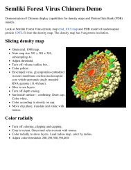
400 kV image data of HSV-1 capsids
500 Å
Joanita Jakana

16
14
12
10
Joanita Jakana
Circularly Averaged Power
8
6
4
2
0
Spectrum
0 1/20 1/10 3/20 1/5 1/4
Spatial frequency (1/Å)

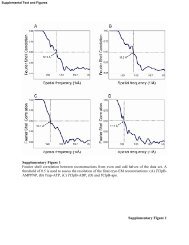
Computed diffraction pattern
F 2 (s) CTF 2 (s) Env 2 (s) + N 2 (s)
Structure factor
Contrast transfer function
Saad et al JSB 133: 32-42 (2001)
Envelope function Background

X-ray Scattering Intensity of HSV-1 Capsids
I x(s)
100
1.5
10
0.5
1.
1
0
-0.5
0.1
2
-1
-1.5
0.02
-2
-2.5
01/500 0.05 1/20 0.1 1/10 0.15 1/6.6 0.2 1/5 0.25
Spatial Frequency (1/Å)
Dr. Hiro Tsuruta at SLAC

X ray Scattering Intensity of GroEL
Resolution (Å)

Computed diffraction pattern
F 2 (s) CTF 2 (s) Env 2 (s) + N 2 (s)
Structure factor
Contrast transfer function
Envelope function Background

Contrast Transfer Function
CTF (s) = - A [(1-Q 2 ) 1/2 sin(γ) + Q cos(γ)]
γ(s) = - 2π (C s λ 3 s 4 /4 - ΔZ λs 2 /2)
ΔZ is vector dependent if there is an astigmatism

Jiang & Chiu Microsc. and Microanal. 7:329-334 (2001)

From F. Thon
Astigmatism

Astigmatism
ΔZ eff (α) = ΔZ m + (ΔZ a sin 2α)/2
ΔZ m = (ΔZ 1 + ΔZ 2 )/2
ΔZ a = ΔZ 1 - ΔZ 2

Synthetic Power Spectrum ∆Z = 0.8µm
Astigmatism
amplitude =
0.0µm
From Wen Jiang
Astigmatism
amplitude =
0.0267µm
Astigmatism
amplitude =
0.1µm

Synthetic Power Spectrum ∆Z = 3 µm
Astigmatism
amplitude =
0.0µm
From Wen Jiang
Astigmatism
amplitude =
0.1µm
Astigmatism
amplitude =
0.375µm

Astigmatism in Single Particle Image
From Dr. Angel Paredes

Computed diffraction pattern
F 2 (s) CTF 2 (s) Env 2 (s) + N 2 (s)
Structure factor
Contrast transfer function
Envelope function Background

EM Envelope Functions : Env(s)
Gaussian type source:
G sc(s) = exp[−π 2 α 2 (C Sλ 2 s 3 − ΔZs) 2 ]
Gaussian type fluctuation:
G tc (s) = exp[ −
π 2
16 ln 2 C 2
λ
2
(
ΔE
C E )2 s 4 ]
Gaussian type fluctuation:
4ln2C 2
λ
2
(
ΔI
C I )2 s 4 ]
Sinusoidal type fluctuation:
G ol (s) = exp[−
π 2
G lm(s) = J O(πΔfλs 2 )
Drift:
G tm(s) = sin(πsΔr)
πsΔr
Chiu Scanning Electron Microsc. 1:569-580 (1978)

Spatial coherence envelope function
1.2
1
0.8
0.6
0.4
0.2
0
0
0.02
1/75 1/20 1/10 1/6.5 1/5.4 1/4.5
0.04
0.06
0.08
0.1
0.12
0.14
0.16
Spatial Frequency (1/Å)
α=.12 mrad
α=.2 mrad
α=.3 mrad
α=.5 mrad
0.18
∆Z=0.5 µm
0.21
0.23

300 keV, Cs = 1.6 mm, defocus = 1 μM
Amplitude
1
0.8
0.6
0.4
0.2
0
-0.2
-0.4
-0.6
-0.8
-1
CTF curve at different illumination angle
0.15 mrad 0.10mrad 0.05mrad
0 0.1 0.2 0.3 0.4 0.5
S(1/Å)

EM Envelope Functions : Env(s)
Gaussian type source:
G sc(s) = exp[−π 2 α 2 (C Sλ 2 s 3 − ΔZs) 2 ]
Gaussian type fluctuation:
G tc (s) = exp[ −
π 2
16 ln 2 C 2
λ
2
(
ΔE
C E )2 s 4 ]
Gaussian type fluctuation:
4ln2C 2
λ
2
(
ΔI
C I )2 s 4 ]
Sinusoidal type fluctuation:
G ol (s) = exp[−
π 2
G lm(s) = J O(πΔfλs 2 )
Drift:
G tm(s) = sin(πsΔr)
πsΔr

Gaussian Approximation for
Cumulative Envelope Function
Env 2 (s) ~ exp (-2BS 2 )

Fitting the spatial coherence envelope
1.2
1
0.8
0.6
0.4
0.2
0
function with exp(-BS 2 )
0
0.01
1/75 1/20 1/10 1/6.5
0.03
0.04
0.06
0.07
0.08
0.1
0.11
0.13
Spatial Frequency (1/Å)
Δz=0.5 μm
Δz=1.μm
Δz=2.0 μm
0.14
0.15
α=0.12 mrad
Exp(-BS 2 )

Computed diffraction pattern
F 2 (s) CTF 2 (s) Env 2 (s) + N 2 (s)
Structure factor
Contrast transfer function
Envelope function Background

Noise Function
N 2 (s) = n 1 exp (n 2 s + n 3 s 2 + n 4 s ½ )

From Dr. Z. Li

Contrast = (F 2 CTF 2 E 2 ) / N 2

200kV Image and Power Spectrum of CPV
Booth JSB 2004
500 A
1/8.6 A
1/8.6 A

JEOL 3000SFF electron cryomicroscope at NCMI
equipped with liquid helium stage and field emission gun

300kV Image Power Spectrum
4.6 Ǻ
156 particles, ΔZ = 0.60 µm
Joanita Jakana, MSA Proceeding, 2004

Experimental B factor vs defocus for 300
kV Images of CPV
Expt B Factor (Å 2 )
200
150
100
50
Joanita Jakana
1 2 3 4
Defocus (µm)

Number of particles
required for a 3-D reconstruction is
inversely proportional to
F 2 (S) exp(-2BS 2 )

I x(s).exp(-2Bs 2 )
0
10-1 -2
-2
10-3 -4
-4
10-5 -6
-6
10-7 -8
-8
10-9 -10
-10
1/20 1/10 1/6.6 1/5 1/4
Spatial Frequency (1/Å)
B=30
B=50
B=100

Causes of High B-Factor
• Large angle of illumination (defocus
dependent)
• Astigmatism (defocus independent)
• Local specimen movement (defocus
independent)
• Insufficient sampling (defocus independent)

Synthetic Power Spectrum ∆Z = 0.8µm
Astigmatism
amplitude =
0.0µm
From Wen Jiang
Astigmatism
amplitude =
0.0267µm
Astigmatism
amplitude =
0.1µm

300kV, Cs=1.6mm
∆Z=0.8 µm astigmatism = 0.0 µm, 0.0267 µm, 0.1µm

Sampling
• Sampling distance in real space :
∆x = ½ - 1/3 expected resolution
• Sampling distance in Fourier space
∆S = 1/(N ∆x)
• Choice of sampling (∆x) and box size (N)
depends on expected resolution and the
defocus used

From Tony Crowther, MRC

Effect of Box Size on CTF Appearance
200 kV, Cs = 1.2mm, 2.8 A/pixel. 96x96 pixels box, ∆Z=5 µm

Effect of Box Size on CTF Appearance
Cs = 1.2 mm
200 kV, Cs = 1.2mm, 2.8 A/pixel. 96x96 pixels box, ∆Z=3 µm

Effect of Box Size on CTF Appearance
200 kV, Cs = 1.2mm, 2.8 A/pixel. 192x192 pixels box, ∆Z=3 µm

Effect of Box Size on CTF Appearance
200 kV, Cs = 1.2mm, 2.8 A/pixel. 288x288 pixels box, ∆Z=3 µm

Vertical error bar: ds = 1/(96*2.8) = 0.00372 Å -1

CCD Camera for Single Particle
Imaging

JEM2010F with a Gatan 4k CCD

MTF of 4k CCD at 200 kV

S/N of 200 kV Carbon Film Image

9Å Map of CPV from CCD Images
Booth et al, JSB 2004

Secondary Structure
Elements in CSP-A
Booth, JSB, 2004

Magnification To Use For Higher
Effective
Microscope
Magnification
55,200
69,000
82,800
110,400
138,000
207,000
Resolution Structure Study
Å/pix
2.71
2.17
1.81
1.35
1.08
0.72
15 microns/pixel Gatan 4k CCD
Dimension of
CCD Frame
on Specimen
(nm)
1,110
886
738
554
443
295
% CCD Frame
Area wrt
82800 x
225
144
100
56
36
16
2/5 Nyquist
(Å)
13.55
10.84
9.03
6.77
5.42
3.61

References
Jiang, W. & Chiu, W. Web-based simulation for contrast transfer function and envelope
functions. Microsc & Microanal 7, 329-334 (2001).
Ludtke, S.J., Jakana, J., Song, J.-L., Chuang, D. & Chiu, W. A 11.5 Å single particle
reconstruction of GroEL using EMAN. J Mol Biol 314, 253-262 (2001).
Saad, A. et al. Fourier amplitude decay of electron cryomicroscopic images of single
particles and effects on structure determination. J Struct Biol 133, 32-42 (2001)
Zhou, Z.H. et al. CTF determination of images of ice-embedded single particles using
a graphics interface. J Struct Biol 116, 216-22 (1996).
Zhu, J., Penczek, P.A., Schroder, R. & Frank, J. Three-dimensional reconstruction with
contrast transfer function correction from energy-filtered cryoelectron
micrographs: procedure and application to the 70S E coli ribosome.
J Struct Biol 118, 197-219 (1997).
Toyoshima, C. & Unwin, P.N.T. Contrast transfer for frozen-hydrated specimens:
Determination from pairs of images. Ultramicroscopy 25, 279-292 (1988).

References
Chiu, W. Factors in high resolution biological structure analysis by conventional
transmission electron microscopy. Scanning Electron Micros 1, 569-580 (1978).
Wade, R.H. & Frank, J. Electron microscope transfer functions for partially coherent
axial illumination and chromatic defocus spread. Optik 49, 81-92 (1977).
Frank, J. Determination of source size and energy spread from electron micrographs
using the method of Young's fringes. Optik 44, 379-91 (1976).
Frank, J. The envelope of electron microscopic transfer functions for partially
coherent illumination. Optik 38, 519-36 (1973).
Thon, F. Phase contrast electron microscopy. in Electron Microscopy in Material
Sciences (ed. Valdre, U.) 571-625 (Academic Press, Inc., New York, 1971).
Erickson, H.P. & Klug, A. The Fourier transform of an electron micrograph: effects of
defocussing and aberrations, and implications for the use of underfocus contrast
enhancement. Phil. Trans. Roy. Soc. Lond. B 261, 105-18 (1970).