A Brief DPL Tutorial

A Brief DPL Tutorial
When you first start DPL you get a four pane window: Project Manager, Session Log
windows on the left, and the two Model windows on the right. (Figure 1)
Figure 1
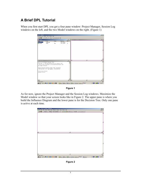
As for now, ignore the Project Manager and the Session Log windows. Maximize the
Model window so that your screen looks like in Figure 2. The upper pane is where you
build the Influence Diagram and the lower pane is for the Decision Tree. Only one pane
is active at each time.
Figure 2
1

Policy Tree
You begin creating your DPL model by inputting data in the Influence Diagram Pane,
and then perfecting your model by adding and adjusting it in the Decision Tree Pane.
After your decision tree is completed, you can run your analysis (“Analysis/Decision
Analysis”) and DPL will create a graphical display of your model – a Policy Tree.
What the Policy Tree does:
♦ Shows the result of your analysis by explicitly displaying every path of the tree.
♦ Fills in the probabilities for each chance event.
♦ Evaluates the Outcome expressions and displays their value under each branch.
♦ Evaluates and displays the Objective Function value in brackets above each
endpoint.
♦ Evaluates and displays the Expected Value of each node, just to the left of each
node, in brackets.
Expected Value
of this node
Get/Pay Value
Objective Function Value
Probability
Figure 3
We will now do a simple example, where there are no uncertainties and we will ignore
the time value of money. You may want to have your copy of DPL up and running on
your computer in order to be able to replicate the steps in the examples.
2

Oil field – A
You own a lease to drill for oil. The oilfield will produce 500.000 barrels of oil per year
for two years, at a cost of $13 per barrel. Drilling costs are $2 million. The expected price
of oil over the next two years is constant at $18. Should you drill for oil?
We will now input this data and create our decision tree.
In the Influence Diagram Pane:
♦ Click on the Decision Node icon to create a Decision Node.
♦ Name this node “Drill Decision”.
♦ Click OK
♦ The corresponding decision tree appears automatically in the Decision Tree Pane
In the Decision Tree Pane:
♦ Double-Click on the Decision Node of the decision tree. The Instance Menu
appears. Choose Asymmetric
♦ Double-Click on the “Yes” branch. The Get/Pay menu pops up.
♦ Insert the formula for the profits: -2000+1000*(18-13)
♦ Click OK
Figure 4
3

Running the Analysis
♦ Click “Analysis / Decision Analysis” on the pull down menu
♦ The Decision Analysis Options menu pops up.
♦ Click OK. The Risk Profile is displayed. Close this window.
♦ The Policy Tree is displayed.
Drill_Decision
[3000]
Yes
[3000]
3000
No [0]
Figure 5
We can see that the optimal decision is to drill the well.
Oil field – B
Let’s suppose now that there is price uncertainty only in year 2. In year 2, the expected
price will be either $22, with a 0.30 probability, $18 with a 0.40 probability or $10.What
is your decision now?
To solve this, we must now insert a chance node and compute Year 1 and Year 2 cash
flows separately. We will make the following modifications to the previous model:
In the Influence Diagram Pane:
♦ Click on the Chance Node icon to create a Chance Node.
♦ Name this node “Year2 Price”
♦ Click on the Data tab
♦ Input the 0.30 probability and the 10 price for the “Low” outcome
♦ Input the 0.40 probability and the 18 price for the “Nominal” outcome
♦ Input the 0.30 probability and the 22 price for the “High” outcome
♦ Click OK
In the Decision Tree Pane:
♦ Click anywhere inside the pane to make this the active pane
4

♦ Click on “Node / Add Chance” in the pull down menu.
♦ Choose “Year2 Price”
♦ Attach this chance node to the upper branch of the “Drill Decision” node
♦ Separate the Year 1 and Year 2 production. Double-Click on the “Yes” branch
of
the “Drill Decision” node. The Get/Pay menu pops up.
♦ Change the formula there to: -2000+500*(18-13)
♦ Click OK
♦ Click on any
branch of the “Year2_Price” node. The Get/Pay menu pops up.
♦ Input the Year 2 cash flow formula: 500*(Year2_Price – 13). You can use the
Variable Icon button in the Get/Pay menu to input the Year2 Price variable
instead of typing it in.
At
this point, your screen should look like Figure 6:
Figure 6
After running the analysis, the policy tree shown in Figure 7:
Drill_Decision
[2400]
Year2_Price
Yes
[2400]
500
No [0]
Figure 7
5

You can double-click on the Year2_Price chance node to expand the branches. After
resizing,
the Policy Tree will now look like Figure 8:
Drill_Decision
[2400]
Yes
It is still optimal to drill.
Year2_Price
[2400]
500
No [0]
Figure 8
Low
.300
Nominal
.400
High
.300
[-1000]
-1500
[3000]
2500
[5000]
4500
Note: To resize the contents
of a window pane at any time, use the “ View / Zoom Full”
command, or click on the corresponding icon.
Oil
field – C
Let’s suppose now
that there is price uncertainty in both years of production. Price in
year
1 will be $14, $18 or $22. Price level of year 2 will depend on year 1 prices. The
Year 1 prices will be increased by $4, remain at the same level, or decrease by $6.
Assume that all probabilities are 0.25, 0.50 and 0.25.
We must now insert a second chance node in our model.
But first, go the “Tools /
Options
/ General” pull down menu and change the default probabilities to 0.25, 0.50 and
0.25. Click OK.
In the Influence Diagram
Pane:
♦ Click on the Chance Node icon to create a Chance Node.
rice”
♦ Name this node “Year1 P
♦ Click on the Data tab
♦ Input the 14 price for the “Low” outcome
♦ Input the 18 price for the “Nominal”
outcome
♦ Input the 22 price for the “High” outcome
6

♦ Click OK
In the Decision Tree Pane:
♦ Click anywhere inside the pane to make this the active pane
♦ Click on the “Year 2”
node with the right side of the mouse.
♦ From the menu that appears choose “Detach”. This will separate
this node from
the rest of the tree.
♦ Click on “Node / Add Chance” in the pull down menu.
♦ Choose “Year1 Price”
♦ Attach this chance node to the upper branch of the “Drill Decision” node. You
may want to move nodes around before doing this in order
to make room for this
additional node.
♦ Reattach the “Year 2 Price” node to the end of the “Year 1 Price” node.
♦ Edit “Year 2 Price” by double clicking on the node.
♦ Go to the Data menu and insert the new probabilities and values for each of the
three branches. Ex: The “Low” outcome branch will have a probability of
0.25
and a value of “Year1 Price – 6”, as this outcome has the effect of lowering the
expected oil price, the “Nominal” branch will be simply “Year1 Price”, and the
“High” branch will be “Year1 Price + 4”.
We must
now adjust our formulas to reflect this new situation:
♦ Click on the “Yes” branch of the “Drill Decision”
node. The Get/Pay menu pops
up.
♦ Change the formula there to: -2000 (this leaves only the investment). Click OK
♦ Click on any branch of the “Year1 Price” node. The Get/Pay menu pops up.
♦ Input
the Year 1 cash flow formula: 500*(Year1_Price–13). You can use the
Variable Icon button in the Get/Pay menu to input the Year1 Price variable
instead of typing it in.
At this point, your screen should
look like Figure 9:
7

Figure 9
After running the analysis, the policy tree is as shown in Figure 10:
Drill_Decision
[2750]
Yes
Year1_Price
[2750]
-2000
No [0]
Low
.250
Nominal
.500
High
.250
Year2_Price
[-1250]
500
Year2_Price
[2750]
2500
Year2_Price
[6750]
4500
Figure 10
8
Low
.250
Nominal
.500
High
.250
Low
.250
Nominal
.500
High
.250
Low
.250
Nominal
.500
High
.250
[-4000]
-2500
[-1000]
500
[1000]
2500
[0]
-500
[3000]
2500
[5000]
4500
[4000]
1500
[7000]
4500
[9000]
6500

Substituting a Get/Pay Expression for an Outcome node
We can also set up the model using a Value Node (Outcome node). This has the
advantage of not cluttering up your tree with large quantity of formulas by assigning
them to specific value nodes. In this example we will substitute both “Get/Pay”
expressions for nodes 1 and 2 for an Outcome, or Value node, which we will define in the
Influence Diagram Pane.
To do this we will create another model in this same file (we could also create a new
file).
In the Project Manager Pane:
♦ Press F12 to go to the Project Manager Pane
♦ Click on the current model (untitled)
♦ Right click with your mouse and choose “Rename” to rename the model to
“Model 1”
♦ Right click again and choose “Duplicate” to create a copy of the model. You are
instantly transported to the Model Pane. Press F12 to return to the Project
Manager Pane.
♦ Rename this new model “Model 2”
♦ Right click again on the model and choose “Make Main” 1
♦ Double click on the model to go to the Model Pane
In the Influence Diagram Pane:
♦ Click on the Value Node icon to create a Value Node.
♦ Name this node “Profits”
♦ Click on the Data tab
♦ Key in the formula for the total Profits from both years: 500*(Year1_Price–13)+
500*(Year2_Price–13). This defines profits for both years
♦ Click OK
1 Note that DPL will run the model that was last set to “main”.
9

In the Decision Tree Pane:
♦ Click on any branch of the Year1_Price. This will bring up the Get/Pay menu.
♦ Delete the formula in the Get/Pay menu.
♦ Repeat this and delete the Get/Pay formula
for the Year2_Price node also. These
formulas are no longer necessary as they are already specified in the Outcome
Node named “Profits”.
♦ Still in Year2_Price node, clic k on the Variable Icon button
menu and choose “Profits”.
in the Get/Pay
♦ Click OK
At this point, your screen should look like Figure 11:
Figure 11
After running the analysis, the policy tree will be identical
to the one shown in Figure 8.
10

Modeling a Lognormal Distribution with a binomial lattice
Rather than inputting all the expected future prices of an asset, we can assume that prices
will follow a certain distribution, and have the model compute what these values will be.
Let’s assume that a NBI Inc’s current stock price is $100, the volatility is 30% per year,
and that stock prices follow a lognormal distribution. We can model these prices with a
t
binomial lattice, where the up state has a value of u e σ
= and d = 1/u. The probability is
rt
e − d
given by p = . We will create a 5 year model (t=1), where r = 5%.
u−d Open a new DPL file. In the Influence Diagram Pane:
♦ Click on the Value Node icon to create a Value Node. We will use these for our
constants.
♦ Name this “u”
♦ Click on the Data tab
♦ Input the formula for u = exp (0.30)
♦ Click Enter and OK
♦ Click on the Value Node icon to create a Value Node.
♦ Name this “d”
♦ Click on the Data tab
♦ Input the formula for d = 1/u
♦ Click Enter and OK
♦ Click on the Value Node icon to create a Value Node.
♦ Name this “r”
♦ Click on the Data
tab
♦ Input the value for r. (0.05)
♦ Click Enter and OK
♦ Click on the Value Node icon to create a Value Node.
♦ Name this “t”
♦ Click on the Data
tab
)
♦ Input the value for t. (1
♦ Click Enter and OK
♦ Click on the Value Node icon to create a Value Node.
♦ Name this “p”
♦ Click on the Data
tab
11

♦ Input the formula for p = [exp(r*t)-d]/(u-d)
♦ Click Enter and OK
♦ Click on the Chance Node icon to create a Chance Node.
♦ Name this node “Yr1”
♦ Modify the outcomes so
♦ Click on the Data tab
♦ Input “p” as the probability
♦ Input $100*u for the “Up” outcome
♦ Input $100*d for the “Down” outcome
♦ Click OK
that we have only two states: “Up” and “Down”
Note that there is no
need to enter the down probability, as the model assumes it is (1-p)
automatically.
We must now create 5 chance nodes that are very similar. The easiest way
to do this is to make a copy of this node and then edit in the modifications. 2
♦ Click on the “Yr1” node
♦ Click “Edit / Copy” and then “Edit / Paste”. A new chance node will appear
♦ Change the name of the new
chance node to “ Yr2”
♦ In the Data tab, replace “100*u” with “Yr1*u” for the “Up” outcome
♦ Replace “100*d” with “Yr1*d” for the “Down” outcome
♦ Click on the “Yr2” node
♦ Click “Edit / Copy” and then “Edit / Paste”. A new chance node will appear
♦ Change the name of the new
chance node to “ Yr3”
♦ In the Data tab, replace “Yr1*u” with “Yr2*u” for the “Up” outcome
♦ Replace “Yr1*d” with “Yr2*d” for the “Down” outcome
Repeat for Chance Nodes “Yr4” and “Yr5”.
In the
Decision Tree Pane:
♦ Click anywhere inside
the pane to make this the active pane
♦ All 5 Chance Nodes are already in place.
♦ Click on any branch of the “Yr1” node. The Get/Pay menu po
♦ Delete the formula there and leave it blank
ps up.
♦ Click OK
♦ Repeat for all chance nodes of the tree except
for the last one (Yr5).
2 Unfortunately this does not work with Student Version 4.0, only with the Full Version
12

At t his point, your screen should look like Figure 12:
The policy tree is shown in Figure 13:
Yr1
[128.403]
Up
.510
Down
.490
Yr2
[164.872]
Yr2
[90.4837]
Up
.510
Down
.490
Yr3
[211.7]
Yr3
[116.183]
Figure 12
Yr4
Up [271.828]
.510
Down
.490
Up
.510
Down
.490
Figure 13
13
Yr4
[149.182]
Yr4
[149.182]
Yr4
[81.8731]
Up
.510
Down
.490
Up
.510
Down
.490
Up
.510
Down
.490
Up
.510
Down
.490
Yr5
[349.034]
Yr5
[191.554]
Yr5
[191.554]
Yr5
[105.127]
Yr5
[191.554]
Yr5
[105.127]
Yr5
[105.127]
Yr5
[57.695]
Up
.510
Down
.490
Up
.510
Down
.490
Up
.510
Down
.490
Up
.510
Down
.490
Up
.510
Down
.490
Up
.510
Down
.490
Up
.510
Down
.490
Up
.510
Down
.490
[448.169]
448.169
[245.96]
245.96
[245.96]
245.96
[134.986]
134.986
[245.96]
245.96
[134.986]
134.986
[134.986]
134.986
[74.0818]
74.0818
[245.96]
245.96
[134.986]
134.986
[134.986]
134.986
[74.0818]
74.0818
[134.986]
134.986
[74.0818]
74.0818
[74.0818]
74.0818
[40.657]
40.657

This tree gives us the distribution of NBI’s stock
five years out. This distribution is
lognormal. We can use this model to calculate the price of options written on this stock.
European
Call Option
Suppose we want to value a European
Call Option on NBI’s stock, with strike price of
180
and 5 years to expiration.
In the Project Manager Pane:
♦ Press F12 to go to the Project Manager Pane
♦ Following the steps explained
previously, create a new model named “European
Call”
♦ Double click on the model to go to the Model Pane
♦ Make this module the “Main” module
In the
Influence Diagram Pane:
♦ Click on the Value Node icon to create a Value Node.
rice”
♦ Name this node “Strike P
♦ Click on the Data tab
♦ Key in 180 for the strike price
♦ Click OK
♦ Click on the Decision Node icon
to create a Decision Node
♦ Name this node “Exercise?”
In the Decision Tree Pane:
♦ Click anywhere inside the pane
to make this the active pane
♦ Click on “Node / Add
Decision” in the pull down menu.
♦ Choose the only option available which is “Exercise?”
♦ Attach this decision node to the “Yr5” chance node
♦ Click on the “Exercise?” node. This will bring up the Ins
♦ Choose “Asymmetric”
tance
Menu
♦ Click on the “Yes” branch of the “Exercise?” node. This will bring up
the
Get/Pay Menu.
♦ Using the Variable Icon button
Strike_Price)/exp(0.05*5)”.
to input the formula “(Yr5 -
3
3 If exercised in year 5, the payoff of the option will be the Year 5 Price less the Strike Price. This
value must be discounted 5 periods at the riskfree rate to arrive at it’s Present Value. If not
exercised, the payoff is zero, which is the automatic assumption of DPL trees whenever no
value or formula is provided in the branch.
14

♦ Click on any branch of the “Yr5” node. This will bring up the Get/Pay
menu.
♦ Delete the formula “Yr5” that is there. Click OK
At this point, your model will look like this (Figure 14):
Figure 14
The policy tree will give the result of 15.6892.
American Call Option
We will now value an American
Call Option on the NBI stock, with strike price of 180
and 5 years to expiration.
We will begin by making a copy of the previous file (European Call) which we will
modify for our purposes, basically
by inserting a Decision Node to exercise or not at each
of the 5 time periods. Rename this file “American Call”.
In the Project Manager Pane:
♦ Delete to “Underlying” model and rename the “European
Call” to “American
Call”
♦ Double click on the model to go to the Model Pane
♦ Make this module the “Main” module
In the Influence Diagram Pane:
♦ For convenience, rename the Value Node “ Strike Price” to “X”.
15

♦ Rename the Decision Node “Exercise?” to “ Exercise5?”
♦ Make four copies of this node (Edit/Copy/Paste)
♦ Rename each of these new Decision Nodes “Exercise1”, Exercise2”, “Exercise3”
and “Exercise4?”
In the
Decision Tree Pane:
We will now insert these new nodes at t=1, t=2, t=3 and t= 4.
♦ Click anywhere inside the pane to make this the active pane
♦ Right Click on the “Yr2” node and choose “Detach”. This will separate this node
from the rest of the tree.
♦ Click on “Node / Add
Decision” in the pull down menu.
♦ Choose “Exercise1”
♦ Attach this
decision node to the “Yr1” chance node
e Menu
♦ Click on the “Exercise1” node. This will bring up the Instanc
♦ Choose “Asymmetric”
♦ Click on the “Yes” branch of the “Exercise1?” node. This will bring up the
Get/Pay Menu.
♦ Input the formula “(Yr1-X)/exp(0.05*1)”.
Click OK.
♦ Drag the “Yr2” node and attach it to the lower (“No” ) branch.
♦ Right Click on the “Yr3”
node and choose “Detach”. This will separate this node
from the rest of the tree.
♦ Click on “Node / Add Decision” in the pull down menu.
♦ Choose “Exercise2”
♦ Attach this decision node to the “Yr2” chance node
♦ Click on the “Exercise2” node. This will bring up the Instance Menu
♦ Choose “Asymmetric”
♦ Click on the “Yes” branch of the “Exercise2?” node. This will bring up the
Get/Pay Menu.
♦ Input the formula “(Yr2-X)/exp(0.05*2)”. Click OK.
♦ Drag the “Yr3” node and
attach it to the lower (“No”) branch.
Repeat this procedure for the last two Decision Nodes. (“Exercise3” and “ Exercise4”)
At this point, your model should look somewhat like in Figure 15:
16

Yr1
Up
Down
Exercise1
Yes
(Yr1-X)/exp(0.05*1)
No
Yr2
Up
Down
Exercise2
Yes
(Yr2-X)/exp(0.05*2)
No
Yr3
Up
Down
Yes
(Yr3 - X)/exp(0.05*3)
No
Exercise3
Figure 15
Up
Yr4
Down
Yes
(Yr4-X)/exp(0.05*4)
No
Exercise4
Yr5
Up
Down
Exercise5
Yes
(Yr5-X)/exp(0.05*5)
The policy tree will give the result of 15.6892. Note that this is the same result as with
the European Option. This was expected, because we know that it is never optimal to
exercise American Options early.
Linking DPL to a Spreadsheet
♦ You can create a spreadsheet in Excel and then have DPL automatically build a
deterministic model from this spreadsheet by linking DPL to this spreadsheet.
Then you can edit your DPL
model to account for chance events and decision
nodes.
♦ Specific DPL variables can be linked
to specific spreadsheet cells
♦ Data can be sent both from DPL to the spreadsheet and from the spreadsheet to
DPL.
♦ In a sensitivity analysis, for example, DPL will send a parameter to the
spreadsheet and request an outcome for that particular scenario, which will then
be returned to DPL as an outcome value.
In the
Spreadsheet:
♦ Start by
setting up your spreadsheet model.
♦ Only named cells will be linked – you must name all input and output cells.
♦ Spreadsheet must be set up to define one scenario only – DPL is the one that will
be doing the sensitivity analysis.
♦ Note that the spreadsheet will function basically as a subroutine of your DPL
model, or a black box – DPL will send data to the
spreadsheet (export link to a
cell with a constant) and get back the result of
a calculation (import link to a cell
with a formula).
Let’s start by building a deterministic model from
a spreadsheet. For this we will use the
spreadsheet
file ChinaOil.xls.
♦ Open a new blank DPL model window
17
No

♦ Click on “Tools / Create Model from Excel”.
♦ Choose the “ChinaOil.xls”
spreadsheet.
♦ Click OK. The Influence Diagram of the model appears.
♦ Click on “Format / Arrange Diagram / Left-to-Right” to rearrange the model on
the screen. (Figure 16)
♦ Run the model by clicking on “Analysis / Decision
Analysis” pull down menu.
♦ DPL will ask which variable to calculate . Use the Variable Icon button to
♦
choose “NPV”. (Since this is a deterministic model with no decision to make,
there is no decision tree.)
In the Risk Profile graph we can see that the expected value is 88 (on the
horizontal scale), the same
as the spreadsheet. This means that there is 0%
probability that the NPV will be less than 88, and 100% probability that the NPV
will be greater or equal 88.
Adding Uncertainty
OperatingCost
FixedCost
DeclineRate
DevelCost
OilPrice
ProdRate
Figure 16
PSCShare
Reserves
♦ We can now add uncertainties to this deterministic model by changing Value
nodes into Chance nodes.
♦ Let’s begin by inserting an uncertainty in the
Oil Price. We do this by changing
this Value node into a chance node.
♦ Right click on the Oil
Price node. Click on “Change Node Type” and choose
“Chance” to change this node into a Chance node.
♦ When the Node Definition window appears, click OK. You will see that the shape
of this node in the Influence
Diagram pane has changed to a circle.
♦ Double click on the Oil Price node again. The Data window will appear.
18
NPV

♦ The three uncertain outcomes (Low, Nominal, High) have the same original value
of $15. We will now change that to $10, $15 and $25
respectively, to cover the
range of possible oil prices for the problem, while maintaining the default
probabilities for now.
♦ Let’s assume that there is also uncertainty over the level of the reserves. Although
the reserves are estimated to be 90MM Bbl it could be as low as 50 or as high
as
200M.
♦ Right click on the Reserves node. Click on “Change Node Type” and choose
“Chance” to change this node into a Chance node.
♦ When the Node Definition window appears, click OK. You will see that the shape
of this node in the Influence Diagram pane has changed to a circle.
♦ Double click on the Reserves node again. The Data window will appear.
♦ The three uncertain outcomes (Low, Nominal, High) still have the same original
value of 90. We will now change that to 50, 90 and $200 respectively and click
OK.
The influence diagram for the model should look somewhat like Figure 17. Notice the
change in shape (and color) of the two nodes we modified from Value to Chance Nodes.
OperatingCost
FixedCost
DeclineRate
DevelCost
OilPrice
ProdRate
Figure 17
PSCShare
♦ We will now run our analysis again, by clicking on “Analysis/Decision Analysis”
on the pull down menu. We get the Policy Tree shown in Figure 18. We can also
see that the Expected NPV of the project has increased from 88 to 175.8 due to
range of possible values for the uncertain variables that we input.
19
Reserves
NPV

OilPrice
[175.835]
Low
.300
Nominal
.400
High
.300
Reserves
[-31.608]
Reserves
[127.906]
Reserves
[447.183]
Figure 18
Determining the relevant Uncertainties
Low
.300
Nominal
.400
High
.300
Low
.300
Nominal
.400
High
.300
Low
.300
Nominal
.400
High
.300
[-63.029]
-63.029
[-42.9486]
-42.9486
[14.9338]
14.9338
[15.1398]
15.1398
[87.9444]
87.9444
[293.954]
293.954
[174.977]
174.977
[350.058]
350.058
[848.888]
848.888
Attempts to model all uncertainties in a project are time consuming and unnecessary, as
not all uncertainties have a relevant effect on the project’s NPV. DPL can help you
determine which uncertainties are relevant by means of a Tornado graph.
♦ Click on “Analysis/Expected Value Tornado Diagram”
♦ In “Value for Sensitivity” choose “Production Rate” and click OK
♦ Enter the low and high values of 0.08 and 0.12.
♦ Click on “Next Value”, choose “Operating Cost” and enter 6 and 11 for the low
and high values.
♦ Click on “Next Value”, choose “Development Cost” and enter 60 and 100 for the
low and high values.
♦ Click on “Next Value”, choose “PSC Share” and enter 0.22 and 0.27 for the low
and high values.
♦ Click on “Run Now”. The Tornado Diagram of Figure 19 indicates that
Operating Cost and Production Rate uncertainties have a much larger impact on
the profitability of the project than Development Costs and PSC Share. This
means you definitely want to model these first two uncertainties, but may pass on
the other less important ones.
20

OperatingCost
ProdRate
DevelCost
PSCShare
Using Utilities
80 100 120 140 160 180 200 220
Figure 19
DPL allows for a very simple means of using a utility function to model risk attitudes.
The Strenlar case is a good example of how the risk attitude as modeled by an utility
function can influence the decision making process.
♦ Open the Strenlar1.da file and run the analysis. We get the Policy Tree shown in
Figure 20 that indicates that the optimal alternative for Mr. X is the riskier of
developing the product on his own.
Strenlar_Decision
[3632]
Develop
Lawsuit
[3632]
-200
Technology
Salary [2017.95]
Technology
Cash_Offer [1004.88]
Figure 20
♦ Now suppose Mr. X is risk averse. A good model for this behavior is an
exponential utility function, which can be totally defined by Mr. X risk tolerance,
which we will assume to be 500.
♦ On the pull down menu, go to “Model/Risk Tolerance” and enter the value of 500.
♦ Run the analysis again. We now get a Policy Tree (Figure 21) that clearly
indicates that given that Mr. X is somewhat risk averse, the optimal course of
action in this case is to go with the less risky alternative of accepting a salary in
the firm plus royalties.
21

Strenlar_Decision
[1113.54]
Develop
Lawsuit
[111.508]
-200
Technology
Salary [1113.54]
Technology
Cash_Offer [926.162]
Figure 21
♦ Now suppose Mr. X risk tolerance is lower, maybe 200. On the pull down menu,
go to “Model/Risk Tolerance” and enter the value of 200 and run the analysis
again.
♦ The new Policy Tree (Figure 22) show that such a low risk tolerance (indicating a
very risk averse attitude) Mr. X should go for the alternative with the lowest risk
of all, mainly the upfront cash offer.
Lawsuit
Develop [-84.7736]
-200
Strenlar_Decision
[790.407]
Technology
Salary [659.817]
Technology
Cash_Offer [790.407]
Figure 22
Note: Values inserted in the Node Data are not automatically added to the tree. They
must be specifically invoked from formulas or a “Get/Pay” expression. Values inserted as
“Get/Pay” are automatically included into the tree calculations.
Linking to spreadsheet
♦ Suppose you linked your DPL model to a spreadsheet and now you want to add an
additional node link. If you just re-link it will delete your whole DPL file
♦ What you want to do is:
♦ Tools/Add linked nodes/From Excel
22

♦ When the window appears, click on the Browse button to re-choose the Excel file to
link
♦ Click “Select”
♦ A new window now appears showing any Excel name that has not yet been linked
♦ Choose the one you want and close all
23