Transformation Invariant Shape Similarity Comparison of Solid Models

Transformation Invariant Shape Similarity Comparison of Solid Models 

Abstract 

David McWherter Mitchell Peabody William C. Regli 

This paper presents two complimentary approaches to comparing 

the shape and topology of solid models. First, we develop a mapping 

of solid models to Model Signature Graphs (MSGs)—labeled, 

undirected graphs that abstract the boundary representation of the 

model and capture relevant shape and engineering attributes. Model 

Signature Graphs are then used to define metric spaces over arbitrary 

sets of solid models. This paper introduces two MSG metric 

spaces: first, a euclidean distance measure via a mapping of MSGs 

to a high-dimension vector space; second, an edit distance measure 

between model signature graphs based on spectral graph theory. 

In practice, exact computation of the edit distance between 

model signature graphs is believed to be an NP-hard problem. We 

show that properties of the design signature graph’s spectra, derived 

from the eigenvalues of its adjacency matrix, can be used as a efficient 

and tractable approximation of the edit distance. Lastly, we 

provide empirical results using real test data from the National Design 

Repository (http://www.designrepository.org) 

to validate the approach. We argue comparisons among solid models 

in these metric space are immune to problems caused by inexactness 

and ambiguity arising from basic modeling transformations 

(scale, translation, rotation, sheer, etc.). It is our belief that this 

work contributes to a growing body of techniques for comparing 

models and indexing CAD media types in database systems. 

Keywords: Similarity Assessment of Solid Models, Shape 

Matching, Design for Manufacture, Variational Process Planning. 

1 Introduction 

Solid models have become integral to modern design and manufacturing. 

As a byproduct of the legacy of manufacturing processes 

are collections of these models which represent various products at 

assorted stages of completion. In order to understand this data, and 

¡ 

http://www.mcs.drexel.edu/¢ URL: regli; Email: 

regli@drexel.edu. 

Geometric and Intelligent Computing Laboratory 

Department of Mathematics and Computer Science 

Drexel University 

3141 Chestnut Street 

Philadelphia, PA 19104 

http://gicl.mcs.drexel.edu/ 

Ali Shokoufandeh 

the relationships between models, it is essential to perform similarity 

assessments between them. 

Primarily, similarity assessments are done in either a one-to-one 

or a one-to-many basis. One-to-one comparisons between models 

can be used to further understand the relationship and similarities 

between two objects. These analyses would be useful in discovering 

whether two parts may share manufacturing techniques, or 

share design substructures. One-to-many comparisons would find 

usage in database applications, in which one model is compared to 

a set of other models in the database. 

We develop a representation of solid models as an attributed 

graph based on a common boundary-representation (BRep) for 

solid models, called Model Signature Graphs (MSG). We then make 

use of this graph representation in order to compute the similarity of 

the solid models. We put forth two similarity measurements based 

on MSGs, one based on structural graph invariants, and the other 

based on techniques of spectral graph theory. 

2 Background and Related Work 

2.1 Similarity Assessment of Solid Models 

Wysk et al. [18] have examined solid model similarity assessment 

using boundary-representations of the models being compared. 

Their approach, to construct a graph that describes the adjacency 

of faces in the solid model, is very similar to ours. Unfortunately, 

their approach has a number of drawbacks which makes 

their similarity assessment less than ideal. First, the system is only 

capable of handling polyhedral objects—more complicated objects 

involving smooth curved surfaces must be approximated with planar 

surfaces. Additionally, the similarity measure that is used is 

not symmetric. The measure of similarity between models A and B 

may not necessarily be the same as the similarity between model B 

and A. This problem leads to difficulty in using the similarity measure 

as an aid to index models using common database schemes, 

which rely on symmetry. 

Cicirello and Regli [16, 7, 8] have developed graph-based methods 

for determining whether two models are identical, or exhibit 

substructure similarity. This approach makes use of feature information 

used to construct a solid model, storing it in a canonical 

graph-structure known as a Model Dependency Graph. These structures 

are then compared against each other to determine whether 

they are isomorphic, or have a subgraph isomorphic relationship. 

The central problem with this approach are that it lacks the granularity 

required for practical similarity assessment—it is only able 

to give a boolean response that two graphs are the same, or not. 

Another significant problem is that it is assumed that feature information 

is available, either directly or via a feature recognizer, to 

construct a canonical representation of the model. Unfortunately, 

this information, which describes how a model is constructed, is

For Submission to the 2001 Shape Modeling Conference 

frequently not available in practical databases of solid models, and 

is difficult (if not impossible) to generate from models. 

2.2 Comparisons of Shape Models 

A considerable amount of work has been done in the field of computer 

vision in Shape Recognition of solid objects. Typically, the 

approaches here assume that there is some sensed input of of the 

shape or object being recognized, as well as a database of solid 

models. Geometric Hashing is typically used in shape recognition, 

comparing a simple representation of the structure of the shape being 

examined, and the representations for the models available in 

the database. 

A common approach to computing model similarity in the field 

of computer vision naturally involves making use of a projection of 

the solid model into a 2-dimensional space (such as a photograph), 

where the input signal is compared to the projections of model objects 

in a database. Given that most information about the 3-d (or 

higher dimensional) properties of the model are thrown away in the 

projection phase, techniques that make more use of the system have 

been developed. 

Aspect graphs are a common mechanism for dealing with models 

whose geometry and configuration are completely known. This 

approach computes all possible appearances that an object may take 

when viewed by an observer (commonly using a projection from 3d 

to 2-d space, for instance). These views are stored in a graph 

whose edges associate views when a simple spatial transformation 

may directly transform one view into another. 

Aspect graphs, however, are difficult to compute for arbitrarily 

solid models, and are typically restricted to objects whose boundaries 

can be described by simple polygonal structures or surfaces 

surfaces of revolution. Practical models, however, are much more 

complicated, however, having combinations of smooth, and polygonal 

surfaces. Known techniques for dealing with these more complicated 

systems are computationally intractable [15]. 

2.3 Graph-based Representations 

In the field of pattern recognition, a number of approaches have 

been set forth to determine similarities between graphs. Primarily, 

these approaches are to construct a similarity measurement based 

on metric distance functions. The metric property enables the measurement 

to be used to aid in indexing collections of graph structures 

in database applications. 

Kubica et al. [14] make use of a distance metric known as editdistance. 

Edit distance is defined as the smallest number of edge 

rotations or additions that are needed to transform one graph into 

another graph. Unfortunately, computing this property of a graph 

is believed to be NP-hard, and no well-known approximation algorithms 

exist to compute it with bounded error. 

In addition to similarity measures based on edit-distance, a 

number of researchers make use of similarity measures based on 

the maximal common subgraph shared between two graphs [4]. 

The technique finds the maximal common subgraph between two 

graphs, and computes its size with respect to the size of the graphs 

themselves. This measurement also constitutes a distance metric, 

and is also believed to be NP-hard. Approximation algorithms to 

compute the maximal common subgraph, however, are more readily 

available than those for edit-distance, however. The methodologies 

we develop in this paper provide similarity measures that may 

be used as an approximate distance metric whenever applicable. 

2 

(a) Wireframe (b) Hidden Lines Removed 

� � � 

� � � 

� � � � � � � � � £ ¤ ¥ 

� � � 

�� 

� � � � � 

�� 

� � � 

� � 

� � � 

� � � 

¡ ¡ ¢ 

¦ ¦ § 

� 

£ £ £ 

� � � 

� � � 

� � � � � 

� � 

� � � ¤ ¤ ¥ 

� � � 

� 

�� 

� � � 

� � � 

� � � 

� � � 

� � � 

� � � 

� � � 

� � � 

� � � 

� � � 

� � � 

¨ ¨ © 

� � � 

� � � 

� � � 

� � � 

� � � 

� � � 

� � � 

� � � 

� � � 

� � � 

� � � 

� � � 

� � � 

© � �� 

�� 

� � � § 

� � � 

� � � 

� � � 

� �� 

¥ � 

�� ¨ ¦ ¤ £ 

�� 

� � � 

� � � 

� � � 

� � � � � � 

� � � 

� � � 

�� 

�� 

�� 

�� 

�� 

�� 

�� 

�� 

�� 

�� 

�� 

�� 

�� 

�� 

�� 

�� 

�� 

�� 

�� 

�� 

�� 

�� 

�� 

�� 

�� 

�� 

�� 

�� 

�� 

�� 

�� 

�� 

�� 

�� 

�� 

¦ § ¦ 

� � 

� � � 

� � � 

� � � 

� 

� � � 

� � � 

� � � 

� � � 

� � � 

� � � 

� � � 

� � � 

�� 

¢ ¡ 

�� 

� � � 

© � 

� � � 

� � � 

� � � ¨ 

� � � 

� � � � � 

� � � 

� � � 

� 

� � � � � � 

� � � 

�� 

�� 

� � � 

�� 

� � � 

�� 

� � � 

� � � 

� � � 

� � � 

� � 

� � � 

� 

� � � 

� � � 

� � � 

� � � 

� � � 

� � � 

� � � 

� � � 

� � � 

� � � 

� � � 

� � � 

� � � 

� � � 

� � � 

� � � 

� � � 

� � � 

� � � 

� � � 

� � � 

� � �� 

� 

� � � 

� � �� 

�� 

� � � 

�� 

� � � 

� � � 

� � 

� � � � 

� � � 

� � � 

� � � 

� � � 

� � � 

� � � 

� � � 

�� 

�� 

� � � 

� � � � � 

� 

� � � 

� � � 

�� 

� � � 

�� 

�� 

� � � 

� � � 

� � � 

� � � 

� � � 

�� 

� � � 

�¢£¤ �� 

�� 

�� 

�� 

�� 

�� 

� � 

� � �� 

�� 

� � �� 

�� 

�� 

� 

�� 

� � � 

�� 

�� 

�� 

�� 

� � � 

� � 

�� 

� 

�� 

�� 

� � � 

� � � 

� � � 

� � � 

� � � 

� � � 

� � � 

� � 

� � � 

� 

� � � 

�� 

� � � 

�� 

� � � � � � 

�� 

� � � 

� � � 

� � � 

� � � � � � 

�� 

�� 

�� 

�� 

�� 

�� 

�� 

�� 

�� 

�� 

�� 

�� 

� � ¥¦§ � 

� � � 

� 

� � � 

� � ¡ �� 

� 

� � �� 

� 

� � � � � � 

� � � 

��¨©� 

�� 

�� 

�� 

� � � 

� � � 

�� 

� � � 

�� 

�� 

�� 

� � � 

�� 

�� 

�� 

�� 

�� 

�� 

�� 

�� 

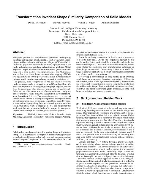
(c) Model Signature Graph 

Figure 1: Representations of the Torpedo model as a solid model 

and MSG. 

3 Problem Statement and Technical Approach 

3.1 Model Signature Graphs 

We make use of a specialized graph structure in order to represent 

solid models in order to perform similarity comparisons. This structure, 

called a Model Signature Graph (MSG), is constructed from 

the boundary representation of a solid model in a manner similar 

to that by Wysk et al. [18] and the Attributed Adjacency Graph 

(AAG) structures used to perform Feature Recognition from solid 

models [13]. 

The boundary representation (BRep) [12] essentially consists of 

a set of edges and a set of faces used by the solid modeler to describe 

the shape of the model in 3-dimensional space. An MSG 

for a solid model � 

is defined as a labeled �� graph, , 

where each face �� 

� 

�� 

�� 

� � � 

�� 

�� 

� � � 

� � � 

� � � 

� � � 

�� 

�� 

is represented as a vertex �� , with at- 

tributes that further describe the qualities of the face in the model. 

For instance, we record the type of the surface (e.g., flat or curved), 

the relative size, and other physical attributes of the face with the 

vertex, including: 

1. topological identifier for the face (planar, conical, etc.); 

2. underlying geometric representation of the surface, i.e. the 

type of function describing the surface; 

�� 

�� 

� � � 

� � �


3. surface area, � ¡£¢¥¤¦¡ , for the face; 

4. set of surface normals or aspects for � . 

An MSG edge § � � exists whenever two faces 

�©¨ �� 

� � � 

� 

� adjacent—i.e., when � ¨ and � � meet at an edge � in the 

� ¨ 

BRep. The MSG edge § � � � � is attributed with features rep- 

� ¨ 

resenting the type of � BRep edge, , connection that is being used, 

including: 

1. topological identifier for the edge � in the model � 

2. concavity/convexity of � ; 

3. underlying geometric representation of the curve of � , i.e. the 

type of function describing the curve; 

4. the length of the curve of � . 

Thus, MSGs are representable as undirected graphs with labeled 

edges and vertices. MSGs are capable of representing either individual 

parts or collections of parts—the connected components 

within the MSG each represent one of the parts making up the collection. 

There is no significant restriction on the attributes stored 

on the vertices and edges in a MSG. The selection to be used in 

applied systems will most likely be tailored to meet the needs of 

the particular application. We assume that for the most part, little 

information aside from the BRep is available for the construction 

of MSGs. 

These attributes represent a substantial amount of the structure 

contained within common BRep models, and will enhance model 

comparisons by aiding in the differentiation of edges and faces in 

the models. In addition, the attributes are easily computed from 

BRep models, which make them extremely practical. 

We believe that some attributes, such as the modeling features 

that are used to generate faces and edges in the BRep, may be 

very important in the matching process during practical use. Unfortunately, 

deriving this information from pure BRep data is an 

extremely difficult process, and may not be worth the gains in performance 

of the similarity measures. Further work must be done 

before we incorporate such attributes in our MSGs for comparisons. 

Example. Figure 2.3 illustrates a transformation from the 

boundary representation of the solid model for a torpedo motor into 

a Model Signature Graph. The complexity of the relationships between 

the faces and edges in the BRep of this model gives a good 

idea of the difficulty of performing shape similarity based on BRep 

data. Good practical algorithms in the research literature for determining 

the similarity of adjacency structures of this form are scarce. 

Making use of MSGs for similarity assessment proves to be an extremely 

challenging problem to solve. 

3.2 Metric Spaces of Solid Models 

A metric space is a collection of objects along with a distance function, 

� �� , known as the metric, which computes a distance between 

any two elements in the set. The distance function � �� must 

satisfy a few conditions: 

�� Identity 

� 

�� £� �� Positivity 

� 

�� Symmetry 

� 

� �� £� �� Triangle Equality 

A collection of objects may naturally have more than one distance 

function, inducing a number of metric spaces that are able to 

be constructed over the objects. 

; 

3 

The constraints provided by the distance metric provides a significant 

amount of structure that can be exploited when working 

with metric spaces. Recently, in the field of databases and indexing, 

a large amount of research has been put forth to store data in metric 

spaces using various tree-structures [3, 6, 10] for efficient search 

and retrieval. Additionally, clustering and knowledge-discovery 

techniques such as � -means or � -median make use of metric distance 

functions to order and discover patterns and statistical distribution 

of data. 

We believe that a number of metric distance functions can be 

used to perform similarity assessment of the shapes of solid models. 

These functions constitute a “plug-in” module that can be tailored 

to perform a wide range of similarity measures based on the nature 

of the application. 

In order to make use of distance metrics in a practical system, 

they must be relatively easy to compute. The algorithmic complexity 

in computing distance metrics for arbitrarily-formed graph 

structures is unfortunately an open question. 

Given a machine to compute a distance metric between two 

graphs, one can trivially decide whether two graphs are isomorphic. 

They are isomorphic if and only if the distance between them 

is zero. As a result, graph isomorphism is Turing-reducible to the 

computation of any graph distance metric, and asymptotic computing 

time will be related to the complexity of algorithms to compute 

graph isomorphism. 

Graph isomorphism is a problem that has been studied for 

decades due to its wide range of applications. Despite the large 

amount of energy spent on the problem, no algorithm has been 

developed that has reduced its worst-case running time to subexponential. 

Surprisingly, it is also unknown whether the problem 

is truly NP-hard or not. 

The difficulties involved in understanding and solving the graph 

distance metric problem dictates the development of approximation 

algorithms to efficiently compute distances between Model Signature 

Graphs. 

3.3 Graph Invariance Vectors 

The eventual aim of our work is to enable indexing and quick retrieval 

of a large repository of CAD models. Although, a measure 

such as edit distance provides a proven metric for graph similarity, 

the cost of running the algorithm is much too high for a database 

that could potentially consist of thousands of designs. Using graph 

invariants, we can form groups, or clusters of potentially isomorphic 

graphs, or graphs that are close enough in similarity to satisfy a 

query. Since the goal of this paper is simply to show that clustering 

based on invariants is a useful means to an end, various clustering 

methods have been chosen to illustrate feasibility. Run-time is not 

an issue at this point, the primary interest being whether or not the 

clustering provides suitable results for further research. 

The graph invariants that we focus on are directly related to the 

degree sequence of a graph. The degree sequence, while not the 

most powerful invariant known, is easily computable, and can be 

exploited to recover general structural properties of the graph. We 

attempt to construct these invariants such that they are normalized, 

and do not depend on differences of scale in the number of edges or 

vertices. The following graph invariants were chosen for inclusion 

in our system: 

1. Vertex and Edge Count—Trivially computable graph invariants. 

Unfortunately, they reveal practically no information 

about the graph structure, and may be weighted too strongly in 

the comparisons we perform, skewing our similarity metrics. 

2. Minimum and Maximum Degree—Provide a measurement 

of the maximum and minimum number of adjacencies between 

one face and the other faces in the model.


3. Median and Mode Degree—Provides a measurement that 

represents statistically the most common and “average” cardinalities 

of adjacencies between faces in a model. 

4. Diameter – The longest path of edge/face crossings between 

any two faces in the model. 

5. Type Histogram – Each model BRep contains a set of faces 

and edges which have various types and features. The analysis 

and statistical breakdown of these component types is used to 

further generate a representation of the model. 

A set of graph invariants can be used to tell if two graphs have 

the potential to be isomorphic or not, but can not be used to give a 

definitive answer. To clarify, if the invariants of two graphs are different, 

there is no way the graphs can be isomorphic; if the invariants 

are all equal, then the graphs may or may not be isomorphic. 

We encode a fixed set of invariants as an Invariant Topology Vector 

(ITV). ITVs gives us the ability to determine a “position” for a 

graph in the metric space relative to other graphs. Graphs with similar 

values for invariants will lie in the same region of the metric 

space. 

Using graph invariants helps prune out graphs which have no 

similarity to a given graph and does not depend on the application of 

the technique. However, we would like to be able to tailor it in some 

fashion to a particular domain to aid in more precise measurements. 

In generating the MSG from the model, we put labels on the 

vertices and edges. We would like to use these values in our ITV 

to give even finer granularity in our assessment. However, since 

there are varying numbers of vertices and edges in the graphs, the 

labels can not be used directly. The ACIS Solid Modeler from Spatial 

Technologies is the modeling system used in our experiments. 

ACIS has 13 different surface types, and 8 different curve types. We 

modify the definition of the ITV to include 21 additional values. In 

effect, we create a histogram of the number of times particular surface 

and edge types occur in the model. Thus, the ITV is a point in 

29 dimensions. 

3.4 EigenDistance 

We primarily focus on techniques of spectral graph theory as a basis 

to approximate graph similarity. Spectral graph theory is the 

study of the adjacency matrix of graphs using linear algebra — particularly 

the study of their eigenvalues and how they relate to other 

properties and features of a graph. 

The spectrum of a graph—the sorted eigenvalues of its adjacency 

matrix, holds a tremendous amount of information related to the 

structure and the topology of a graph. It has been used in numerous 

applications for the purposes of graph partitioning [11] and geometric 

hashing in vision recognition [17]. 

There are a number of different adjacency matrices that are used 

in spectral graph theory to generate a graph’s spectrum. Biggs [2], 

for instance, uses a common form: 

� if � is adjacent to � 

�� 

otherwise. � 

�� 

Chung [5], proposes the use of an alternative “normalized” form 

of the graph adjacency matrix, which takes into consideration the 

degrees of the vertices in the graph to determine the entries in the 

matrix. This form, known as the graph Laplacian, has eigenvalues 

that have well-known and powerful relationships with other graph 

properties, such as the graph diameter. The Laplacian is formally 

defined as follows: 

�� 

�� 

�� 

� � 

�� 

� 

� � if �� 

� ¨ 

� 

� 

and 

� 

� 

if � and � are adjacent, 

� �� 

�� otherwise. 

�� , 

� 

4 

In addition to the relationship between the Laplacian spectrum and 

other graph invariants, as well as the fact that the normalization 

helps to reduce the effect of irregular degrees on graph vertices, we 

chose to make use of the Laplacian matrix for our approach. 

3.4.1 Spectral Hashing 

A primary goal of the distance metric is to ensure that two identical 

graphs have no distance between them. In addition, two graphs 

with only minor differences should consistently be measured relatively 

closely. To achieve this requirement, we first compute the 

eigenvalue spectrum of the graph. This operation can be done during 

a preprocessing phase, and the results stored for later use, if a 

model of reference Model Signature Graphs are being used in an 

application. From this point on, we consider this spectrum to be a 

projection of the graph from the space of graphs to �� , and we use 

this space as a basis for most distance computations that make up 

the metric. 

Distance computations between the image of graphs in � � are 

done using any one of a number of vector-based metric norms. In 

particular, are investigating the use of �� , �� , and other norms. 

3.4.2 Substructure Comparison 

A reasonable measure of similarity between graphs relies on the 

concept of shared substructure [4]. Semantically, two graphs that 

have similar common substructures themselves will tend to be similar. 

We believe that substructure similarity is central to most practical 

applications of shape recognition. 

We make use of substructure information in the following manner. 

After computing the eigenvalue spectrum for a graph, we partition 

the graph into two or more subgraphs, removing the edges that 

cross the partition(s). If this is done wisely, it will isolate highly 

connected component graphs at each level of the recursion. We 

generate the eigenvalue spectrum for each component, and recursively 

partition and index again. 

Optimally partitioning a graph to minimize the number (or 

weight) of the edges that cross the partition is itself an NP-hard 

problem. In order to make the problem more tractable, we make 

use of an approximation to partitioning using the eigenvalues that 

were computed for the graph. The technique, known as Spectral 

Graph Partitioning, puts the ��¦� vertices into one of two subgraphs 

based on the sign of the corresponding entry in the eigenvector corresponding 

to the second smallest eigenvalue (also known as the 

Fiedler Vector). Thus, with little added asymptotic complexity, the 

graph can be decomposed into two halves, and the process may be 

repeated. 

4 An Example 

We apply the techniques discussed to construct the ITVs and eigenvalue 

spectra required to perform distance computations on a simple 

model available in the National Design Repository [1], to 

demonstrate the transformations we use to perform shape recognition 

and matching. We will employ the solid model depicted in 

Figure 2: the spinner3 model, a simple practical model found in 

industry with an extremely simple BRep. 

ITV. First, we compute the ITV associated with the model. The 

following table depicts the graph invariant attributes associated with 

the MSG for spinner3:


� 

� 

� 

�� 

� ¨ �� ¨ �� ¨ �� ¨�� ¨�� ¨�� ¨ �� ¨ �� ¨ �� ¨ �� ¨�� ¨ �� ¨ �� ¨ �� ¨�� 

��¨�� 

� � 

¨�� 

�� 

�� 

� 

� 

�� 

� 

�� 

�� ¨�� ¨��¨�� 

� �� ¨ �� ¨ �� 

�� ¨ �� ¨ �� 

�� ¨ �� ¨�� 

�� 

� ��¨ � 

�� 

�� ¨ �� ¨ �� ¨�� ¨�� 

�� ¨ �� 

�� 

� 

�� ¨�� 

� ¨�� 

� ��¨ � 

�� 

�� ¨�� ¨ �� ¨�� 

�� ¨�� ¨ �� 

� 

¨�� ¨ �� 

� �� 

� �� ¨�� 

�� ¨�� ¨�� ¨ �� ¨�� 

�� ¨�� ¨ �� 

�� ¨�� ¨ �� ¨ �� 

�� 

¨�� ¨ �� 

�� ¨�� ¨ �� 

�� 

¨�� ¨ �� 

�� ¨�� ¨�� 

�� 

�� ¨�� 

�� ¨ 

�� 

� �� 

� � �� 

�� 

� �� 

� 

� � � 

� � 

� 

� � � 

� � 

� 

� � � 

� � 

� 

� � � 

� � 

� 

� � � 

� � 

� 

�� 

� �� 

Figure 3: Laplacian matrix and eigenvalue spectrum computed for the spinner3 model. 

�� 

��¥� 

�� 

�� 

�� 

�� 

�� 

Figure 2: An example of our approach: encoding of the spinner3 

model into an MSG, which is then used to create the ITV and 

EigenDistance vector spaces. 

Attribute Value 

Vertex Count 24 

Edge Count 63 

Degree Max 2 

Degree Min 17 

Degree Mode 4 

Degree Median 4.00 

Degree Std. Deviation 3.27 

Graph Diameter 3 

The computation of these attributes is relatively straightforward. 

The only attribute that we are currently concerned with that is not 

computable in time linear in the number of edges is the graph diameter. 

We are able to compute graph diameter in two ways. In 

one implementation, the diameter is computed using an all-pairs 

shortest-path algorithm, such as the Floyd-Warshall algorithm [9], 

5 

which can be computed in � �� , for graphs of � �� vertices. An 

alternative method uses an upper bound for the diameter, computed 

from the eigenvalue spectra [5]. This upper bound is stated as follows: 

� 

�� 

��¥�� ¥��©�� 

�©�� ©� 

� 

where � � is the � -th largest eigenvalue in the eigenvalue spectrum, 

and � is the number of eigenvalues in the spectrum (which is equal 

to the number of vertices in the graph). We investigate the use of 

this as an approximation of graph diameter as if both our eigenvalue 

metric and the invariance metrics are being used, the computation 

of graph diameter is done at effectively no added cost. 

Eigenvalue Metric. In order to compute the eigenvalue similarity 

measure we must first compute the Laplacian matrix for the 

spinner3 model, and then compute its eigenvalue spectrum. Both 

the Laplacian matrix ( � 

� 

), and the eigenvalue spectrum ( � ) com- 

puted from the spinner3 model are depicted in Figure 3. We compute 

the eigenvalues of the system with software packages that use 

a Householder-�� matrix diagonalization algorithm, which efficiently 

generates the eigenvalues in time cubic in the number of 

vertices of the graph. 

The ITV and the eigenvalue vector can be compared using standard 

vector norms in � � . In the case of comparing graph spectra, 

small provisions must be made for comparing graphs with differing 

number of vertices, as spectrum vectors of different lengths must 

be compared. Currently, we simply remove the smallest eigenvalues 

from the larger vector, and compute standard �� (Euclidean) 

and �� norms. 

5 Empirical Results 

We investigate the application of the � measures on models found 

in the National Design Repository [1]. We� have � computed the 

distances between each a collection of models using both � 

the 

�� ¦�� eigenvalue spectrum similarity measure ), � 

and 

(�� 

the (�� ¦�� graph invariant topology vector measure ). The 

computations that we have done make use of a 

�¦�� 

�� 

�� 

� 

�� 

�� 

�� 

�� 

�� 

�� 

�� 

�� 

� 

�


��¨�£�� 

�¨� ��£�� 

��¨�£�� 

�¨� ��£�� 

�¨�� 

��¦� �� 

��¦�£�� 

£¢¥¤ ¦¨§ ©��¨�� 

��¡ 

��¥�� 

�� 

��£�¥� �¨� ��¨�� 

�� 

�£� ��¨�� 

�¨�¡�£�¥� 

Figure 4: Similarity comparison between spinner3, spinner4, and part01. 

��¥�� 

��£�¥�� ¨� ��¨�� 

�� 

�¨� ��¨�� 

�¨��¨�� 

�� ¨�� 

��¨�� 

�¨� �� 

��¨�� 

�� 

��¥�� 

£¢¥¤�� ¦¨§ ©�¢��¨ �� 

��¡ 

�¨� ��¥�� 

�¨��¥�� 

Figure 5: Similarity comparison between Team Part-1, Team Part-2, and 3tmount. 

non-recursive version of the method, which we expect limits its 

ability to do substructure similarity assessment. Figures 4, 5, 6, 

and 7 depict the similarity measures between triples of models that 

we have selected to highlight various properties of our approaches. 

Example 1. The first triplet of models, shown in Figure 4, is 

made up of parts known as part01, spinner3, and spinner4. These 

are fairly simple industrial models, and their relationship under both 

distance measures is illustrated in Figure 4. Visually, one would 

expect that spinner3 and spinner4 would be more similar to one 

another, which is contradictory to the results attained by both of 

our similarity metrics. More interestingly, this is consistent for 

both similarity measures. Our interpretation is that the measures 

are picking up on a similarity in the model complexity in spinner3 

and part01, given that spinner4 is a noticeably more complex part 

with a greater number of geometric and topological entities. 

Example 2. The second triple, shown in Figure 5, consists of 

models from the US Department of Energy’s Technologies Enabling 

Agile Manufacturing (TEAM) Program. The Team Part- 

1, Team Part-2, and 3tmount. Team Part-1 and Team Part-2 are 

6 

benchmark parts made to test process planning applications, exhibit 

striking similarity, although their scales and orientation in the 

Repository are different. 3tmount is an actual model from industry, 

and is considerably different from either Team Part-1 or Team Part- 

2. As is depicted in Figure 5, the distance measures seem to agree 

with visual intuition. The Team Part-1 and Team Part-2 models are 

considered to be far more similar than 3tmount. 

Example 3. The third set of models is made up of STI-Simple, 

STI-Boeing, and Chamber, and are shown in Figure 6. These parts 

are taken from industry, the first two contributed to the Design 

Repository by the Boeing Aircraft Company. Note that they exhibit 

slightly more complexity than is found in the first sets of models. 

To the human observer, STI-Simple and STI-Boeing are variations 

on a common structure, whereas the Chamber is an extremely different 

model, whose curves and shape bears little resemblance to 

the other two. The distance measures also appear to correlate with 

visual intuition. In addition, it may be noted that the distances computed 

between Chamber and the other two parts are extremely similar. 

This is likely to be due to the fact that there is largely a 1-to-1 

correspondence between faces and edges in the STI models, which


makes their MSGs extremely similar. 

�� 

��¥�� ¢¡¤£¦¥¨§�© �¨� 

�� 

�� ¨�� ¢�¤�¦�¨�� 

�� 

��¥�� ¥�� 

�� 

�� 

�¥�� 

�� 

�� 

��¨�� ¥� �� 

�� 

�¥� �� 

�¥�� 

Figure 6: Similarity comparison between STI-Boeing, STI-Simple, and Chamber. 

��¦�� 

�¢��¤� �� ¨�� 

�� 

�� ¨�� 

��¤� 

�¢��¤� �� ¨�� ¤��¨��¨� �� 

�� 

�� ¨�� ¨�� 

��¤� 

��¦�� ¤�� 

��¦�� 

�¢�� ¨�� 

�� 

�� ¨�� ¨��¨� �� 

�� 

Figure 7: Similarity comparison between ToolingBlock, ToolingBlock-1, and ToolingPlate. 

Example 4. The final set of models we examine is made up of 

ToolingBlock, ToolingBlock-1, and ToolingPlate, and are shown in 

Figure 7. These are also industrial fixturing models, but they have 

a large amount of detail on multiple scales, made up primarily of 

general shape, then of the many small holes on each surface. The 

distances between these models does not appear to follow human 

intuition on the large-scale, on which ToolingBlock would be extremely 

similar to ToolingBlock-1, as opposed to ToolingPlate. To 

mimic human interpretation in this example, filtering of some form 

must be applied to perform multi-scaled comparisons of the models. 

Although not readily apparent in the figures, each of these parts 

is stored in the Design Repository [1] with differing scales, and 

transformations. It is essential to note that our similarity measures 

have no difficulty performing the comparisons between the objects 

7 

based purely on their shape and structure, regardless of these transformations. 

The selected comparisons illustrate the metric properties of our 

similarity measures. Take, for example, � 

the � 

comparison between 

Team Part-1, Team Part-2, and 3tmount. Tables 4 and 4 � 

provides 

verification that the triangle inequality is obeyed by both the 

similarity measures. 

�¦�� 

�� 

�� 

�¦�� and �� 

The central conclusion is that the “length” of the path between 

two models that passes through an intermediate is longer than the 

direct path between the models. This is a realization of the triangle 

inequality, and is a key property of our distance measures. 

It should be noted that our similarity measures only approximate 

metric functions, and models may be found for which the triangle 

inequality does not hold.


A B C 

1 part01 spinner3 spinner4 �� 

EigD(A,B) + � 

�� 

EigD(B,C) 

EigD(B,C) + � 

��¦�� 

EigD(C,A) 

EigD(C,A) + � 

�� 

EigD(A,B) 

� 

� 

� 

�� 

�� 

�� 

� � 

�� 

�� ©� �� 

� � � � � 

� 

�� ©� � 

�� 

�� 

�� 

� 

2 

3 

4 

Team Part-1 

STI-Simple 

ToolingBlock 

Team Part-2 

STI-Boeing 

ToolingBlock-1 

3tmount 

Chamber 

ToolingPlate 

A B C 

Table 1: Verification of the triangle inequality for �� 

ITVD(A,B) + ITVD(B,C) � 

��¤�� 

�� 

�¦�� . 

ITVD(B,C) + � 

��¦�� 

ITVD(C,A) 

�� 

ITVD(C,A) + ITVD(A,B) � 

� � � � 

� 

� � � �� ©� � 

1 � 

part01 � 

spinner3 spinner4 �� 

�� 

� 

2 Team Part-1 Team Part-2 3tmount 

�� 

3 

4 

STI-Simple 

ToolingBlock 

STI-Boeing 

ToolingBlock-1 

Chamber 

ToolingPlate 

6 Discussion and Conclusions 

��¤��¤�� 

�� 

� � � �� 

�� ©� ��©� �� 

� �� 

Table 2: Verification of the triangle inequality for �� 

We have demonstrated two approaches to compute the similarity 

between solid models, based on shape and topology. Both techniques 

make use of a transformation from solid models to graphbased 

structures, called Model Signature Graphs, and then project 

these graphs into a vector space for easy comparison. The distance 

between images of models in the vector spaces using normal vector 

norms is used as a basis for determining model similarity. We 

have shown that the similarity metrics reflect real-world concepts 

of model differences, which makes them applicable when a similarity 

assessment that mimics human capabilities of shape recognition. 

The measurements also have the property that they approximate 

metric distance functions, which enable them to be used as a 

means for indexing solid models for efficient retrieval. 

Future Work. We foresee two major aspects of the 

� 

� 

�� ¦�� method that needs further development. 

�� 

Further refining the technique of recursive subdivision of the 

measure to aid in identifying substructure similarity is essential to 

shape recognition. Additionally, means of comparing eigenvalue 

spectra with a differing number of elements may be done in a 

more intelligent manner, that does not throw away � information, 

or artificially inflate the differences between graphs with a large 

difference in the number of vertices. 

With respect to further development of the �� 

ric, we believe that the attribute lists that are used in the ITVs may 

be further refined, to eliminate interdependence of attributes. Other 

graph invariants may also be developed or exploited. Eigenvalue 

spectra, for instance, may be incorporated into the ITVs. Also 

very important will be the development of a weighting of ITV attributes 

to optimize similarity calculations over particular collections 

of models, and to minimize the effects of attributes which 

contain little information. 

Finally, we plan to apply our similarity metrics to databases of 

solid models collected from the National Design Repository [1]. 

We believe that the metrics will prove to be extremely useful in 

performing database indexing and clustering of the models for 

knowledge-discovery and data mining (KDD). 

�¦�� met- 

Acknowledgements. This work was supported in part by 

National Science Foundation (NSF) Knowledge and Distributed 

Intelligence in the Information Age (KDI) Initiative Grant 

CISE/IIS-9873005; CAREER Award CISE/IIS-9733545 and Grant 

ENG/DMI-9713718. 

8 

�¦�� . 

Any opinions, findings, and conclusions or recommendations expressed 

in this material are those of the author(s) and do not necessarily 

reflect the views of the National Science Foundation or the 

other supporting government and corporate organizations. 

References 

[1] National design repository. 

http://www.designrepository.org., 2000. 

[2] Norman L. Biggs. Algebraic Graph Theory. Cambridge 

Tracts in Mathematics 67. Cambridge University Press, 1974. 

[3] S. Brin. Near neighbor search in large metric spaces. In Proceedings 

of VLDB 1995, pages 574–584, 1995. 

[4] Horst Bunke and Kim Shearer. On a relation between graph 

edit distance and maximum common subgraph. Pattern 

Recognition Letters, pages 689–694, 1997. 

[5] Fan R. K. Chung. Spectral Graph Theory. Number 92 in 

Regional Conference Series in Mathematics. American Mathematical 

Society, 1997. 

[6] P. Ciaccia, M. Patella, and P. Zezula. M-tree: An efficient 

access method for similarity search in metric spaces. In Proceedings 

of the 23rd VLDB, August 1997. 

[7] Vincent Cicirello and William C. Regli. Resolving nonuniqueness 

in design feature histories. In David Anderson 

and Wim Bronsvoort, editors, Fifth Symposium on Solid Modeling 

and Applications, New York, NY, USA, June 8-11 1999. 

ACM, ACM Press. Ann Arbor, MI. 

[8] Vincent A. Cicirello. Intelligent retrieval of solid models. 

Master’s thesis, Drexel University, Geometric and Intelligent 

Computing Laboratory, Department of Mathematics and 

Computer Science, Philadelphia, PA 19104, June 1999 1999. 

[9] T. H. Corman, C. E. Leiserson, and R. L. Rivest. Introduction 

to Algorithms. MIT Press/McGraw Hill, 1990. 

[10] A. Fu, P. Chan, Y.L. Cheung, and Y.S. Moon. Dynamic vptree 

indexing for n-nearest neighbor search given pair-wise 

distances. VLDB Journal, 9:154–173, 2000.


[11] Bruce Hendrickson and Robert Leland. An improved spectral 

graph partitioning algorithm for mapping parallel computations. 

SIAM Journal on Scientific Computing, 16(2):452–469, 

1995. 

[12] Christopher M. Hoffmann. Geometric and Solid Modeling: 

An Introduction. Morgan Kaufmann Publishers, Inc., California, 

USA, 1989. 

[13] S. Joshi and T. C. Chang. Graph-based heuristics for recognition 

of machined features from a 3D solid model. Computer- 

Aided Design, 20(2):58–66, March 1988. 

[14] Ewa Kubicka, Grzegorz Kubicki, and Ignatios Vakalis. Using 

graph distance in object recognition. In Proceedings of the 

1990 ACM annual conference on Cooperation, pages 43–48, 

February 1990. 

[15] Sylvain Petitjean. The enumerative geometry of projective 

algebraic surfaces and the complexity of aspect graphs. International 

Journal of Computer Vision, 19(3):1–27, 1996. 

[16] William C. Regli and Vincent Cicirello. Managing digital 

libraries for computer-aided design. International Journal 

of Computer Aided Design, 32(2):119–132, Februrary 2000. 

Special Issue on CAD After 2000. Mohsen Rezayat, Guest Editor. 

[17] Ali Shokoufandeh, Sven J. Dickinson, Kaleem Siddiqi, and 

Steven W. Zucker. Indexing using a spectral encoding of topological 

structure. Computer Vision and Pattern Recognition, 

2, 1999. 

[18] Tien-Lung Sun, Chuan-Jun Su, Richard J. Mayer, and 

Richard A. Wysk. Shape similarity assessment of mechanical 

parts based on solid models. In Rajit Gadh, editor, ASME 

Design for Manufacturing Conference, Symposium on Computer 

Integrated Concurrent Design, pages 953–962. ASME, 

Boston, MA. September 17-21. 1995. 

9

Transformation Invariant Shape Similarity Comparison of Solid Models

Create successful ePaper yourself

Delete template?

Save as template?