Kastelyn's Formula for Perfect Matchings

Kastelyn’s Formula for Perfect Matchings
Rich Schwartz
February 6, 2012
1 Pfaffian Orientations on Planar Graphs
The purpose of these notes is to prove Kastelyn’s formula for the number of
perfect matchings in a planar graph. For ease of exposition, I’ll prove the
formula in the case when G has the following description: G can be drawn
inside a polygon P such that P −G is a finite union of smaller polygons. I’ll
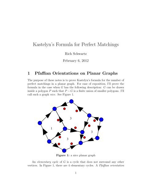
call such a graph nice. See Figure 1.
1
3
3
Figure 1: a nice planar graph
An elementary cycle of G is a cycle that does not surround any other
vertices. In Figure 1, there are 4 elementary cycles. A Pfaffian orientation
1
3

on G is a choice of orientations for each edge such that there are an odd number
of clockwise edges on each elementary cycle. Figure 1 shows a Pfaffian
orientation. The red dots indicate the clockwise edges, with respect to each
elementary cycle.
Lemma 1.1 Any nice graph has a Pfaffian orientation.
Proof: Choose a spanning tree T for G and orient the edges of T arbitrarily.
Define a dual graph as follows. Place one vertex in the interior of each
elementary cycle of G, and a root vertex for the outside of the big polygon,
and then connect the vertices by an edge if they cross an edge not in T. Call
this dual graph T ∗ . If T ∗ is not connected, then T contains a cycle. Since
T contains a cycle, T ∗ is connected. If T ∗ contains a cycle, then T is not
connected. Since T is connected, T ∗ contains no cycle. In short T ∗ is a tree.
Let v be any node of T ∗ . The vertex v joins to an edge w of T ∗ across an
edge e ∗ . The edge e ∗ crosses one edge e of the corresponding elementary cycle
of G. Orient e so that this cycle has an odd number of clockwise oriented
edges, then cross off v and e ∗ , leaving a smaller tree. Now repeat, using a
node of the smaller tree. And so on. At each step, there is one way to orient
the edge to make things work for the current elementary cycle. ♠
Figure 2: the trees T and T ∗ .
2

2 Kastelyn’s Theorem
Let G be a nice graph with a Pfaffian orientation. Assume that G has an
even number of vertices. Let v1,...,v2n be the vertices of G. Let A denote
the signed adjacency matrix of G. This means that
• Aij = 0 if no edge joins vi to vj.
• Aij = 1 if the edge joining vi to vj is oriented from vi to vj.
• Aij = −1 if the edge joining vi to vj is oriented from vj to vi.
A perfect matching of G is a collection of edges e1,...,en of G such that
every vertex belongs to exactly one ej. Let P(G) denote the number of
distinct perfect matchings of G. These notes are devoted to proving:
Theorem 2.1 (Kastelyn) P(G) =
�
|det(A)|.
Let A t denote the transpose of a matrix A. The matrix A is called skewsymmetric
if A t = −A. This is equivalent to the condition Aij = −Aji for
all i,j. By construction, the signed adjacency matrix A is skew-symmetric.
Let A be a 2n×2n skew symmetric matrix. The Pfaffian of A is defined
as the sum
p(A) = 1
2 n n!
� n�
sign(σ) Aσ(2i−1),σ(2i). (1)
σ i=1
The sum is taken over all permutations of the set {1,...,2n}.
Below, we’ll prove the following result, known as Muir’s Identity.
(p(A)) 2 = det(A). (2)
GivenMuir’sIdentity,Kastelyn’sTheoremcanbereformulatedasfollows.
Theorem 2.2 Let G be a nice graph, equipped with any Pfaffian orientation.
Let A be the corresponding signed adjacency matrix. Then P(G) = |p(A)|.
First I’ll prove Theorem 2.2 and then I’ll derive Muir’s Identity.
3

3 Proof Theorem 2.2
Given that A is a skew-symmetric matrix, there is some redundancy in the
definition of the Pfaffian. We write our permutations as
(1,...,2n) → (i1,j1,i2,j2,...,in,jn). (3)
Say that two permutations are equivalent if one can get from one to the
other by permuting the (i,j) pairs and/or switching elements within the
pairs. Each equivalence class of permutations has 2 n n! members. Moreover,
each equivalence class has a unique member such that i1 < ... < in and
ik < jk for all k. Let S denote the set of these special permutations.
Two equivalent permutations contribute the same term in p(A), thanks
to the skew symmetry of A. Therefore, we have the alternate definition
p(A) = � n�
sign(σ) Aσ(2i−1),σ(2i). (4)
σ∈S i=1
The terms in Equation 4 are in one-to-one correspondence with the perfect
matchings. To prove Theorem 2.2, we just have to prove that all such
terms have the same sign. Let s(M) be the term of Equation 4 corresponding
to the perfect matching M. We orient the edges of M according to the
Pfaffian orientation. Call an edge of M bad if it points from a higher indexed
vertextoalowerindexedvertex. Thesignofs(M)justdependsontheparity
of the number of bad edges. We just have to prove that every two perfect
matchings M1 and M2 have the same parity of bad edges.
The symmetric difference M1∆M2 is a finite union of (alternating) cycles
of even length. We can produce a new perfect matching M ′ by switching the
matching on one or more of the cycles of M1∆M2. Thus, M1 and M2 can
be “joined” by a chain of perfect matchings, each of which differ by a single
even alternating cycle. Hence, it suffices to consider the case when M1∆M2
is a single cycle C.
If we permute the indices of G and recompute the signs, all permutations
change by the same global sign. So, it suffices to consider the case when the
vertices of C are given as 1,...,2k in counterclockwise order. The edges of
M1|C are (12), (34), etc. so the bad edges of M1|C are precisely the clockwise
edges. If M1|C has an odd (even) number of bad edges then M1|C has an
odd (even) number of clockwise edges. The edges of M2|C are (23), (45), ...,
(k1). Hence, if M2|C has an odd (even) number of bad edges then M2|C has
an even (odd) number of clockwise edges.
4

The cycle C surrounds some edges common to M1 and M2. Therefore C
surrounds an even number of vertices. Below we will prove that C must have
an odd number of clockwise edges. Hence, the number of clockwise edges in
the two cases has opposite parity. Hence, the number of bad edges in the
two cases has the same parity. Hence s(M1) = s(M2).
The following Lemma completes the proof of Theorem 2.2.
Lemma 3.1 (Kastelyn) Suppose that C is a cycle that surrounds an even
number of vertices. Then C has an odd number of clockwise edges.
Proof: Let n(C) denote the number of clockwise edges of C plus the number
of vertices contained in the interior of the region bounded by C. It suffices
to prove that n(C) is always odd.
Every nice planar graph G ′ can be extended to a triangulated disk G,
and every Pfaffian orientation on G ′ extends to a Pfaffian orientation on G.
(When each new edge is drawn, breaking up an elementary cycle, there is a
unique way to orient the edge to keep the condition on the two smaller cycles
that are created.) So, it suffices to prove this result when C is the boundary
of a triangulated disk ∆.
There are two cases to consider, Suppose ∆ has an interior edge e which
joins two vertices of C. Then we can write ∆ = ∆1 ∪∆2, where ∆1 and ∆2
are two smaller disks joined along e. Let Cj be the boundary of ∆j. Here
we have n(C)−1 = n(C1)+n(C2) because e is counted exactly once on the
right hand side. In this case, we see by induction that n(C) is odd.
The remaining case to consider is when ∆ has a triangle T having an
edge on C and one interior vertex, as shown in Figure 3. In this case, let and
∆ ′ = ∆ −T. Let C ′ be the boundary of ∆ ′ . A short case by case analysis
shows that N(C) = N(C ′ ) or N(C) = N(C ′ )−2. The result again holds by
induction. ♠
T
Figure 3: Chopping off a triangle
5

4 Muir’s Identity
The remainder of these notes is devoted to proving Muir’s Identity.
Call the matrix A special if it has the form
⎡
⎤
M1 0 ... 0 0 0
⎢ 0 M2 0 ... 0 0 ⎥
A = ⎢
⎥
⎣ 0 0 M3 0 ... 0⎦
...
, Mk
�
0
=
−ak
�
ak
0
From Equation 4 we have p(A) = a1...an. Also det(A) = (a1...an) 2 . So,
Muir’s identity holds when A is a special matrix.
Below we will prove
Lemma 4.1 Let X denote the set of all 2n×2n skew symmetric matrices.
There is an open S ⊂ X with the following property. If A ∈ S then there is
a rotation B (depending on A) such that BAB −1 is a special matrix.
After we prove Lemma 4.1, we will establish the following transformation
law. If B is any 2n×2n matrix, then
(5)
p(BAB t ) = det(B)p(A). (6)
Let A ∈ S, the set from Lemma 4.1. We have
(p(A) 2 ) = 1 (p(BAB −1 )) 2 = 2 det(BAB −1 ) = 3 det(A).
Equality 1 comes from the Equation 6 and from the fact that B t = B −1
when B is a rotation. Equality 2 is Muir’s identity for special matrices.
Equality 3 is a familiar fact about determinants. Since Muir’s identity is a
polynomialidentity,andholdsonanopensubsetofskew-symmetricmatrices,
the identity holds for all skew-symmetric matrices.
5 Proof of Lemma 4.1
The best way to do this is to work over the complex numbers, and then drop
back down to the reals at the end.
Let 〈,〉 be the standard Hermitian form on C 2n . That is
〈(z1,...,z2n),(w1,...,w2n)〉 =
6
2n�
i=1
ziwi. (7)

Here, the bar denotes complex conjugation. Here are some basic properties
of this object.
• When v,w ∈ R 2n , we have 〈v,w〉 = v · w. So, the Hermitian form is
kind of an enhancement of the dot product.
• 〈v,w〉 = 〈v,w〉.
• 〈av1 +v2,w〉 = a〈v1,w〉+〈v2,w〉.
• LetM ∗ denotetheconjugatetransposeofM. Then〈Mv,w〉 = 〈v,M ∗ w〉.
These properties will be used in the next lemma.
Lemma 5.1 If A is real and skew symmetric (so that A ∗ = −A) then the
eigenvalues of A are pure imaginary.
Proof: Let λ be an eigenvalue and v a corresponding eigenvector. We have
λ〈v,v〉 = 〈Av,v〉 = 〈v,A ∗ v〉 = 〈v,−λv〉 = −λ〈v,v〉. (8)
Hence λ = −λ. This is only possible if λ is pure imaginary. ♠
Let S denote the set of real skew-symmetric matrices having eigenvalues
of the form λ1,λ1,...,λn,λn, where 0 < |λ1| < ... < |λn|. Note that S is
nonempty, because one can easily construct a special matrix in S. Note also
that S is open, because the eigenvalues vary continuously. So, S contains a
nonempty open set.
Let A be any element of S. Let Ek ⊂ C 2n denote the subspace of vectors
of the form av+bw where A(v) = λk(v) and B(w) = λk(w). By construction,
Ek is a 2-dimensional subspace over C.
Lemma 5.2 Suppose i �= j. If v ∈ Ei and w ∈ Ej then 〈v,w〉 = 0.
Proof: It suffices to prove that 〈v1,v2〉 = 0 when v1 and v2 are eigenvalues
of A corresponding to eigenvalues having different magnitudes. We have
λ1〈v1,v2〉 = 〈A(v1),v2〉 = 〈v1,A ∗ (v2)〉 = −〈v1,A(v2)〉 = −λ2〈v1,v2〉.
Hence, either |λ1| = |λ2| or 〈v1,v2〉 = 0. ♠
Let Vk = Ek ∩R 2n .
7

Lemma 5.3 Vk is 2-dimensional as a real vector space.
Proof: Note that Ek is invariant under complex conjugation. Vk is at least 2
dimensional because it contains all vectors of the form v+v with v ∈ Ek. On
the other hand Vk cannot be more than 2-dimensional because the C-span
of Vk is contained in Ek. ♠
For real vectors v,w, recall that 〈v,w〉 is just the dot product. Hence
v · w = 0 when v ∈ Vi and w ∈ Vj. So the n planes V1,...,Vn are pairwise
perpendicular. Note also that A(Vk) = Vk. So, we have succeeded in finding
n pairwise perpendicular and A-invariant 2-planes in R 2n .
Lemma 5.4 A acts on each Vk as a dilation by |λk| followed by a 90 degree
rotation.
Proof: Note that A 2 has all negative real eigenvalues. On Ek, we have
A 2 (v) = −|λk| 2 (v). The lemma follows immediately from this. ♠
Now for the end of the proof: Given the properties of V1,...,Vn, we can
find a rotation B such that
B(Vk) = Wk := span(e2k−1,e2k), k = 1,...,n. (9)
The map BAB −1 preserves Wk and acts on Wk as the composition of a
dilation and a 90 degree rotation. From here, it is easy to see that BAB −1
must be a special matrix.
6 The Transformation Law
6.1 Brute Force Approach
By an obvious scaling argument, it suffices to establis Step 1 when det(B) =
1. As is well known from Gaussian elimination, every such B is the product
of elementary matrices. Using the fact that det(E1E2) = det(E1)det(E2), it
suffices to establish Step 1 for elementary calculations. This is a fairly easy
calculation which you might prefer to the more abstract argument given
below.
8

6.2 The Main Argument
Let V = R 2n and let V ∗ denote the dual space. Let e1 ,...,e 2n denote the
standard basis for V ∗ .
Given the skew-symmetric matrix A, introduce the 2-form
[A] = �
i

6.3 Forms
Now I’ll give details on tensors which should explain the argument above.
Let V = R 2n . Let V ∗ denote the vector space of linear functions from V
to R. The space V ∗ is called the dual of V. A canonical basis for V ∗ is given
by e 1 ,...,e 2n , where e j is the function such that
A k-tensor is a map φ : V ×...×V → R such that
e j (a1,...,a2n) = aj. (14)
φ(∗,...,∗,av+w,∗,...,∗) = aφ(∗,...,∗,v,∗,...,∗)+φ(∗,...,∗,w,∗,...,∗). (15)
In other words, if you hold all positions fixed but one, then φ is a linear
function of the remaining variable. The product V ×...×V is supposed to
be the k-fold product.
The k-tensor φ is said to be a k-form if
φ(∗,...,∗,ai,∗,...,∗,aj,∗,...,∗) = −φ(∗,...,∗,aj,∗,...,∗,ai,∗,...,∗). (16)
In other words, if you switch two of the entries, the sign changes.
If φ1 and φ2 are k-forms, then so are rφ1 and φ1+φ2. In other words, the
set of all k-forms makes a vector space. This vector space is denoted ∧ k (V).
A nice element of ∧ k (V) is given by
ω = e i1 ∧...∧e ik , i1 < ... < ik. (17)
This tensor has the following description. If we want to evaluate ω(v1,...,vk),
we make a 2n × k matrix having rows v1,...,vk. Then we take the square
minor made from columns i1,...,ik, then we take the determinant of this
minor. Familiar properties of the determinant guarantee that ω really is a
k-form. Call ω an elementary k-form.
Lemma 6.2 The elementary k-forms make a basis for ∧ k (V).
Proof: Anyk-formisdeterminedbywhatitdoestothek-tuples(ei1,...,eik ),
as the indices range over all possibilities. Hence, the elementary forms span
∧k (V). Also, the form ei1 ik ∧...∧e assigns 1 to (ei1,...,eik ) and 0 to all other
such lists. Hence this particular elementary k-form is not a linear combination
of the others. But this means that the elementary k-forms are linearly
independent. ♠
10

6.4 The Wedge Product
Now we know that ∧ k (V) has dimension 2n choose k. In particular, ∧ 2n (V)
has dimension 1: all 2n-forms are multiples of e 1 ∧...∧e 2n .
Given two lists I = {i1 < ... < ia} and J = {j1 < ... < jb}, let K denote
the sorted list of I ∪J. We define
• σ(I,J) = 0 if I ∩J �= ∅.
• σ(I,J) = 1 if an even permutation sorts the elements i1,...,ia,j1,...,jb.
• σ(I,J) = −1ifanoddpermutationsortstheelementsi1,...,ia,j1,...,jb.
There is a bi-linear map
defined as follows.
∧ : ∧ a (V)×∧ b (V) (18)
(e i1 ∧...∧e ia )∧(e j1 ∧...∧e jb ) = σ(I,J)e k1 ∧...∧e ka+b . (19)
The map is extended to all of ∧ a (V) × ∧ b (V) using bi-linearity. This map
is known as the wedge product. The wedge product is associative, so that
(α∧β)∧γ = α∧(β ∧γ).
Another formula for the wedge product is
α∧β(v1,...,va,wa+1,...,wa+b) =
1 �
sign(σ)α(vσ(1),...,vσ(a))×β(wσ(a1),...,wσ(a+b)) (20)
(a+b)! σ
The sum is over all permutations of the set 1,...,a + b. The (×) in this
equation is just ordinary multiplication. One can check, using properties of
determinants, that this formula holds when α and β are elementary forms.
Then, the general case follows from the linearity of Equation 20.
As in the short version of Step 1, we define [A] ∈ ∧2 (V) to be the 2-form
[A] = �
i

6.5 Transformation Laws
Nothing we say here has to do with the dimension being even, so we set
m = 2n and remark that everything works for m odd as well. Suppose that
T is a linear transformation and ω is a k-form. We have the general definition
As a special example, we have
T ∗ (ω)(v1,...,vk) = ω(T(v1),...,T(vk)). (22)
T ∗ (e 1 ∧...∧e m )(e1,...,em) = e 1 ∧...∧e m (T(e1,...,t(2m)) =
� �
σ
e 1 ∧...∧e m
�
�
T1jej,..., �
�
Tnjej =
sign(σ) �
�
Ti,σ(i) e 1 ∧...∧e m = det(T)e 1 ∧...∧e m .
The sum is taken over all permutations. Since ∧ m (V) is 1-dimensional,
and the pull back operation respects scaling, we have the simpler formula
T ∗ (ω) = det(T)ω, (23)
for any m-form. This explains Equality 1 in Equation 13.
It is an easy consequence of Equation 20 that
T ∗ (α∧β) = T ∗ (α)∧T ∗ (β). (24)
From the associativity of the wedge product, we get
T ∗ (α1 ∧...∧αk) = T ∗ (α1)∧...∧T ∗ (αk). (25)
This explains Equality 2 in Equation 13.
12