Optimal Designs for the Prediction of Individual Effects in Random ...
Optimal Designs for the Prediction of Individual Effects in Random ...
Optimal Designs for the Prediction of Individual Effects in Random ...

Create successful ePaper yourself
Turn your PDF publications into a flip-book with our unique Google optimized e-Paper software.
<strong>Optimal</strong> <strong>Designs</strong> <strong>for</strong> <strong>the</strong> <strong>Prediction</strong> <strong>of</strong> <strong>Individual</strong><br />
<strong>Effects</strong> <strong>in</strong> <strong>Random</strong> Coefficient Regression<br />
Maryna Prus and Ra<strong>in</strong>er Schwabe<br />
Abstract In this note we propose optimal designs <strong>for</strong> <strong>the</strong> prediction <strong>of</strong> <strong>the</strong> <strong>in</strong>dividual<br />
responses as well as <strong>for</strong> <strong>the</strong> <strong>in</strong>dividual deviations from <strong>the</strong> population mean response<br />
<strong>in</strong> random coefficient models. In this situation <strong>the</strong> mean population parameters are<br />
assumed to be unknown such that <strong>the</strong> per<strong>for</strong>mance measures <strong>of</strong> <strong>the</strong> prediction do<br />
not co<strong>in</strong>cide <strong>for</strong> both objectives and, hence, <strong>the</strong> design optimization lead to substantially<br />
diverse results. For simplicity we consider <strong>the</strong> case, where all <strong>in</strong>dividuals are<br />
treated <strong>in</strong> <strong>the</strong> same way. If <strong>the</strong> population parameters were known, Bayesian optimal<br />
designs would be optimal (Gladitz and Pilz,1982). While <strong>the</strong> optimal design <strong>for</strong><br />
<strong>the</strong> prediction <strong>of</strong> <strong>the</strong> <strong>in</strong>dividual responses differ from <strong>the</strong> Bayesian optimal design<br />
propagated <strong>in</strong> <strong>the</strong> literature (Prus and Schwabe, 2011), <strong>the</strong> latter designs rema<strong>in</strong> <strong>the</strong>ir<br />
optimality, if only <strong>the</strong> <strong>in</strong>dividual deviations from <strong>the</strong> mean response are <strong>of</strong> <strong>in</strong>terest.<br />
1 Introduction<br />
<strong>Random</strong> coefficient regression models, which <strong>in</strong>corporate variations between <strong>in</strong>dividuals,<br />
are gett<strong>in</strong>g more and more popular <strong>in</strong> many fields <strong>of</strong> application, especially<br />
<strong>in</strong> biosciences. The problem <strong>of</strong> optimal designs <strong>for</strong> estimation <strong>of</strong> <strong>the</strong> mean population<br />
parameters <strong>in</strong> <strong>the</strong>se models has been widely considered and many <strong>the</strong>oretical<br />
and practical solutions are available <strong>in</strong> <strong>the</strong> literature. More recently prediction <strong>of</strong><br />
<strong>the</strong> <strong>in</strong>dividual response as well as <strong>of</strong> <strong>the</strong> <strong>in</strong>dividual deviations from <strong>the</strong> population<br />
mean response attracts larger <strong>in</strong>terest <strong>in</strong> order to create <strong>in</strong>dividualized medication<br />
and <strong>in</strong>dividualized medical diagnostics or to provide <strong>in</strong><strong>for</strong>mation <strong>for</strong> <strong>in</strong>dividual se-<br />
Maryna Prus<br />
Institute <strong>for</strong> Ma<strong>the</strong>matical Stochastics, Otto-von-Guericke University, Universitätsplatz 2, 39106<br />
Magdeburg, Germany, e-mail: maryna.prus@ovgu.de<br />
Ra<strong>in</strong>er Schwabe<br />
Institute <strong>for</strong> Ma<strong>the</strong>matical Stochastics, Otto-von-Guericke University, Universitätsplatz 2, 39106<br />
Magdeburg, Germany, e-mail: ra<strong>in</strong>er.schwabe@ovgu.de<br />
1
2 Maryna Prus and Ra<strong>in</strong>er Schwabe<br />
lection <strong>in</strong> animal breed<strong>in</strong>g, respectively. The frequently applied <strong>the</strong>ory developed by<br />
Gladitz and Pilz (1982) <strong>for</strong> determ<strong>in</strong><strong>in</strong>g designs, which are optimal <strong>for</strong> prediction,<br />
requires <strong>the</strong> prior knowledge <strong>of</strong> <strong>the</strong> population parameters, which can be useful if pilot<br />
experiments are available. In this note we consider <strong>the</strong> practically more relevant<br />
situation, where <strong>the</strong> population parameters are unknown.<br />
The paper is organized as follows: In <strong>the</strong> second section <strong>the</strong> model will be specified<br />
and <strong>the</strong> prediction <strong>of</strong> <strong>in</strong>dividual effects will be <strong>in</strong>troduced. Section three provides<br />
some <strong>the</strong>oretical results <strong>for</strong> <strong>the</strong> determ<strong>in</strong>ation <strong>of</strong> optimal designs, which will<br />
be illustrated <strong>in</strong> section 4 by a simple example. The f<strong>in</strong>al section presents some<br />
discussion and conclusions.<br />
2 Model Specification and <strong>Prediction</strong><br />
In <strong>the</strong> general case <strong>of</strong> random coefficient regression models <strong>the</strong> observations are<br />
assumed to result from a hierarchical (l<strong>in</strong>ear) model: At <strong>the</strong> <strong>in</strong>dividual level <strong>the</strong> jth<br />
observation <strong>of</strong> <strong>in</strong>dividual i is given by<br />
Yi j = f(xi j) ⊤ β i + εi j, xi j ∈ X , j = 1,..,mi, i = 1,..,n, (1)<br />
where n denotes <strong>the</strong> number <strong>of</strong> <strong>in</strong>dividuals, mi is <strong>the</strong> number <strong>of</strong> observations<br />
at <strong>in</strong>dividual i, f = ( f1,.., fp) ⊤ is <strong>the</strong> vector <strong>of</strong> known regression functions, and<br />
β i = (βi1,..,βip) ⊤ is <strong>the</strong> <strong>in</strong>dividual parameter vector specify<strong>in</strong>g <strong>the</strong> <strong>in</strong>dividual response.<br />
The experimental sett<strong>in</strong>gs xi j may be chosen from a given experimental region<br />
X . With<strong>in</strong> an <strong>in</strong>dividual <strong>the</strong> observations are assumed to be uncorrelated given<br />
<strong>the</strong> <strong>in</strong>dividual parameters. The observational errors εi j have zero mean E(εi j) = 0<br />
and are homoscedastic with common variance Var(εi j) = σ 2 .<br />
At <strong>the</strong> population level <strong>the</strong> <strong>in</strong>dividual parameters β i are assumed to have an unknown<br />
population mean E(β i ) = β and a given covariance matrix Cov(β i ) = σ 2 D.<br />
All <strong>in</strong>dividual parameters and all observational errors are assumed to be uncorrelated.<br />
The model can be represented alternatively <strong>in</strong> <strong>the</strong> follow<strong>in</strong>g <strong>for</strong>m<br />
Yi j = f(x j) ⊤ β + f(x j) ⊤ bi + εi j<br />
by separation <strong>of</strong> <strong>the</strong> random <strong>in</strong>dividual deviations bi = β i − β from <strong>the</strong> mean response<br />
β. Here <strong>the</strong>se <strong>in</strong>dividual deviations bi have zero mean E(bi) = 0 and <strong>the</strong><br />
same covariance matrix Cov(bi) = σ 2 D as <strong>the</strong> <strong>in</strong>dividual parameters.<br />
We consider <strong>the</strong> particular case that <strong>the</strong> number <strong>of</strong> observations as well as <strong>the</strong> experimental<br />
sett<strong>in</strong>gs are <strong>the</strong> same <strong>for</strong> all <strong>in</strong>dividuals (mi = m and xi j = x j). Moreover,<br />
we assume <strong>for</strong> simplicity that <strong>the</strong> covariance matrix D is regular. The s<strong>in</strong>gular case<br />
will be addressed shortly <strong>in</strong> <strong>the</strong> discussion.<br />
In <strong>the</strong> follow<strong>in</strong>g we <strong>in</strong>vestigate both <strong>the</strong> predictors <strong>of</strong> <strong>the</strong> <strong>in</strong>dividual parameters<br />
β 1 ,...,β n and <strong>of</strong> <strong>the</strong> <strong>in</strong>dividual deviations b1,...,bn.<br />
(2)
<strong>Optimal</strong> <strong>Designs</strong> <strong>for</strong> <strong>Prediction</strong> <strong>of</strong> <strong>Individual</strong> <strong>Effects</strong> 3<br />
As shown <strong>in</strong> Prus and Schwabe (2011), <strong>the</strong> best l<strong>in</strong>ear unbiased predictor ˆ β i <strong>of</strong><br />
<strong>the</strong> <strong>in</strong>dividual parameter β i is a weighted average <strong>of</strong> <strong>the</strong> <strong>in</strong>dividualized estimate<br />
ˆβ i;<strong>in</strong>d = (F ⊤ F) −1 F ⊤ Yi, based on <strong>the</strong> observations at <strong>in</strong>dividual i, and <strong>the</strong> estimator<br />
<strong>of</strong> <strong>the</strong> population mean ˆ β = (F ⊤ F) −1 F ⊤ ¯Y,<br />
ˆβ i = D((F ⊤ F) −1 + D) −1 ˆ β i;<strong>in</strong>d + (F ⊤ F) −1 ((F ⊤ F) −1 + D) −1 ˆ β. (3)<br />
Here F = (f(x1),...,f(xm)) ⊤ denotes <strong>the</strong> <strong>in</strong>dividual design matrix, which is equal <strong>for</strong><br />
all <strong>in</strong>dividuals, Yi = (Yi1,...,Yim) ⊤ is <strong>the</strong> observation vector <strong>for</strong> <strong>in</strong>dividual i, and<br />
¯Y = 1 n ∑n i=1 Yi is <strong>the</strong> average response across all <strong>in</strong>dividuals.<br />
It is worth-while mention<strong>in</strong>g that <strong>the</strong> estimator <strong>of</strong> <strong>the</strong> population mean may be<br />
represented as <strong>the</strong> average ˆ β = 1 n ∑n i=1 ˆ β i;<strong>in</strong>d <strong>of</strong> <strong>the</strong> <strong>in</strong>dividualized estimates and does,<br />
hence, not require <strong>the</strong> knowledge <strong>of</strong> <strong>the</strong> dispersion matrix D, whereas <strong>the</strong> predictor<br />
<strong>of</strong> <strong>the</strong> <strong>in</strong>dividual parameter β i does.<br />
The per<strong>for</strong>mance <strong>of</strong> <strong>the</strong> prediction (3) may be measured <strong>in</strong> terms <strong>of</strong> <strong>the</strong> mean<br />
squared error matrix <strong>of</strong> ( ˆ β ⊤<br />
1 ,..., ˆ β ⊤<br />
n )⊤ . Us<strong>in</strong>g results <strong>of</strong> Henderson (1975) it can be<br />
shown that this mean squared error matrix is a weighted average <strong>of</strong> <strong>the</strong> correspond<strong>in</strong>g<br />
covariance matrix <strong>in</strong> <strong>the</strong> fixed effects model and <strong>the</strong> Bayesian one,<br />
MSE β = σ 2 ((In − 1 n 1n1 ⊤ n ) ⊗ (F ⊤ F + D −1 ) −1 + ( 1 n 1n1 ⊤ n ) ⊗ (F ⊤ F) −1 ), (4)<br />
where In is <strong>the</strong> n × n identity matrix, 1n is a n-dimensional vector <strong>of</strong> ones and “⊗”<br />
denotes <strong>the</strong> Kronecker product <strong>of</strong> matrices as usual. Note that this representation<br />
slightly differs from that given <strong>in</strong> Fedorov and Hackl (1997, section 5.2).<br />
Similarly <strong>the</strong> best l<strong>in</strong>ear unbiased predictor ˆbi = ˆ β i − ˆ β <strong>of</strong> <strong>the</strong> <strong>in</strong>dividual deviation<br />
bi can be alternatively represented as a scaled difference<br />
ˆbi = D((F ⊤ F) −1 + D) −1 ( ˆ β i;<strong>in</strong>d − ˆ β) (5)<br />
<strong>of</strong> <strong>the</strong> <strong>in</strong>dividualized estimate ˆ β i;<strong>in</strong>d from <strong>the</strong> estimated population mean ˆ β. The<br />
correspond<strong>in</strong>g mean squared error matrix <strong>of</strong> <strong>the</strong> prediction <strong>of</strong> <strong>in</strong>dividual deviations<br />
(ˆb ⊤ 1 ,..., ˆb ⊤ n ) ⊤ can be written as a weighted average <strong>of</strong> <strong>the</strong> covariance matrix <strong>of</strong> <strong>the</strong><br />
prediction <strong>in</strong> <strong>the</strong> Bayesian model and <strong>the</strong> dispersion matrix D <strong>of</strong> <strong>the</strong> <strong>in</strong>dividual effects<br />
MSE b = σ 2 ((In − 1 n 1n1 ⊤ n ) ⊗ (F ⊤ F + D −1 ) −1 + ( 1 n 1n1 ⊤ n ) ⊗ D). (6)<br />
Note that <strong>in</strong> <strong>the</strong> case <strong>of</strong> a known population mean β, which was considered by<br />
Gladitz and Pilz (1982), <strong>the</strong> mean squared error matrix <strong>for</strong> <strong>the</strong> prediction <strong>of</strong> <strong>in</strong>dividual<br />
parameters co<strong>in</strong>cides with that <strong>for</strong> <strong>the</strong> prediction <strong>of</strong> <strong>in</strong>dividual deviations, which<br />
equals σ 2 In ⊗ (F ⊤ F + D −1 ) −1 .
4 Maryna Prus and Ra<strong>in</strong>er Schwabe<br />
3 <strong>Optimal</strong> Design<br />
The mean squared error matrix <strong>of</strong> a prediction depends crucially on <strong>the</strong> choice <strong>of</strong><br />
<strong>the</strong> observational sett<strong>in</strong>gs x1,...,xm, which constitute a design and can be chosen<br />
by <strong>the</strong> experimenter to m<strong>in</strong>imize <strong>the</strong> mean squared error matrix <strong>in</strong> a certa<strong>in</strong> sense.<br />
Typically <strong>the</strong> optimal sett<strong>in</strong>gs will be not necessarily all dist<strong>in</strong>ct. Then a design<br />
� �<br />
x1 ,..., xk<br />
ξ =<br />
(7)<br />
w1 ,..., wk<br />
can be specified by its dist<strong>in</strong>ct sett<strong>in</strong>gs x1,...,xk, k ≤ m, say, and <strong>the</strong> correspond<strong>in</strong>g<br />
numbers <strong>of</strong> replications m1,...,mk or <strong>the</strong> correspond<strong>in</strong>g proportions w j = m j/m.<br />
For analytical purposes we make use <strong>of</strong> approximate designs <strong>in</strong> <strong>the</strong> sense <strong>of</strong><br />
Kiefer (see e. g. Kiefer, 1974), <strong>for</strong> which <strong>the</strong> <strong>in</strong>teger condition on mw j is dropped<br />
and <strong>the</strong> weights w j ≥ 0 may be any real numbers satisfy<strong>in</strong>g ∑ k j=1 m j = m. For <strong>the</strong>se<br />
approximated designs <strong>the</strong> standardized <strong>in</strong><strong>for</strong>mation matrix <strong>for</strong> <strong>the</strong> model without<br />
<strong>in</strong>dividual effects (β i ≡ β, i. e. D = 0) is def<strong>in</strong>ed as<br />
M(ξ ) = ∑ k j=1 w jf(x j)f(x j) ⊤ = 1 m F⊤ F. (8)<br />
Fur<strong>the</strong>r we <strong>in</strong>troduce <strong>the</strong> standardized covariance matrix <strong>of</strong> <strong>the</strong> random effects ∆ =<br />
mD <strong>for</strong> notational ease. With <strong>the</strong>se notations we may def<strong>in</strong>e <strong>the</strong> standardized mean<br />
squared error matrices as<br />
MSE β (ξ ) = (In − 1 n 1n1 ⊤ n ) ⊗ (M(ξ ) + ∆ −1 ) −1 + ( 1 n 1n1 ⊤ n ) ⊗ M(ξ ) −1<br />
<strong>for</strong> <strong>the</strong> prediction <strong>of</strong> <strong>the</strong> <strong>in</strong>dividual parameters and<br />
MSE b(ξ ) = (In − 1 n 1n1 ⊤ n ) ⊗ (M(ξ ) + ∆ −1 ) −1 + ( 1 n 1n1 ⊤ n ) ⊗ ∆ (10)<br />
<strong>for</strong> <strong>the</strong> prediction <strong>of</strong> <strong>the</strong> <strong>in</strong>dividual deviations. For any exact design ξ <strong>the</strong> matrices<br />
MSE β (ξ ) and MSE b(ξ ) co<strong>in</strong>cide with <strong>the</strong> mean squared error matrices (4) and (6),<br />
respectively, up to a multiplicative factor σ 2 /m.<br />
In this paper we focus on <strong>the</strong> <strong>in</strong>tegrated mean squared error (IMSE) criterion,<br />
which is def<strong>in</strong>ed, <strong>in</strong> general, as<br />
IMSE β = �<br />
X E(∑n i=1 ( ˆµi(x) − µi(x)) 2 )ν(dx) (11)<br />
<strong>for</strong> prediction <strong>of</strong> <strong>in</strong>dividual parameters, where ˆµi(x) = f(x) ⊤ ˆ β i and µi(x) = f(x) ⊤ β i<br />
denote <strong>the</strong> predicted and <strong>the</strong> true <strong>in</strong>dividual response, and <strong>the</strong> <strong>in</strong>tegration is with<br />
respect to a given weight distribution ν on <strong>the</strong> design region X , which is typically<br />
uni<strong>for</strong>m. The standardized IMSE-criterion Φ β = m<br />
σ 2 IMSE β can be represented as<br />
Φ β (ξ ) = (n − 1)tr((M(ξ ) + ∆ −1 ) −1 V) + tr(M(ξ ) −1 V), (12)<br />
(9)
<strong>Optimal</strong> <strong>Designs</strong> <strong>for</strong> <strong>Prediction</strong> <strong>of</strong> <strong>Individual</strong> <strong>Effects</strong> 5<br />
which is a weighted sum <strong>of</strong> <strong>the</strong> IMSE-criterion <strong>in</strong> <strong>the</strong> fixed effects model and <strong>the</strong><br />
Bayesian IMSE-criterion, where V = �<br />
X f(x)f(x)⊤ν(dx) is <strong>the</strong> “<strong>in</strong><strong>for</strong>mation” <strong>of</strong> <strong>the</strong><br />
weight distribution ν and “tr” denotes <strong>the</strong> trace <strong>of</strong> a matrix.<br />
With <strong>the</strong> general equivalence <strong>the</strong>orem (see e. g. Silvey, 1980) we may obta<strong>in</strong> <strong>the</strong><br />
follow<strong>in</strong>g characterization <strong>of</strong> an optimal design.<br />
Theorem 1. The approximate design ξ ∗ is IMSE-optimal <strong>for</strong> <strong>the</strong> prediction <strong>of</strong> <strong>in</strong>dividual<br />
parameters, if and only if<br />
f(x) ⊤ ((n − 1)(M(ξ ∗ ) + ∆ −1 ) −1 V(M(ξ ∗ ) + ∆ −1 ) −1 + M(ξ ∗ ) −1 VM(ξ ∗ ) −1 )f(x)<br />
≤ tr(((n − 1)(M(ξ ∗ ) + ∆ −1 ) −1 M(ξ ∗ )(M(ξ ∗ ) + ∆ −1 ) −1 + M(ξ ∗ ) −1 )V) (13)<br />
<strong>for</strong> all x ∈ X .<br />
For any experimental sett<strong>in</strong>g x j <strong>of</strong> ξ ∗ with w j > 0 equality holds <strong>in</strong> (13).<br />
The IMSE-criterion <strong>for</strong> <strong>the</strong> prediction <strong>of</strong> <strong>in</strong>dividual deviations is given by<br />
IMSE b(ξ ) = �<br />
X E(∑n i=1 ( ˆµb i (x) − µ b i (x)) 2 )ν(dx), (14)<br />
where ˆµ b i (x) = f(x)⊤ ˆbi and µ b i (x) = f(x)⊤ bi denote <strong>the</strong> predicted and <strong>the</strong> true <strong>in</strong>dividual<br />
response deviation <strong>for</strong>m <strong>the</strong> population mean, respectively. The standardized<br />
IMSE-criterion Φb = m<br />
σ 2 IMSE b can aga<strong>in</strong> be written as<br />
Φb(ξ ) = (n − 1)tr((M(ξ ) + ∆ −1 ) −1 V) + tr(∆V). (15)<br />
The first term <strong>in</strong> (15) co<strong>in</strong>cides with <strong>the</strong> criterion function <strong>of</strong> <strong>the</strong> Bayesian IMSEcriterion<br />
and <strong>the</strong> second term is constant. Hence, Bayesian IMSE-optimal designs<br />
are also IMSE-optimal <strong>for</strong> <strong>the</strong> prediction <strong>of</strong> <strong>in</strong>dividual deviations. The characterization<br />
<strong>of</strong> IMSE-optimal designs is given by <strong>the</strong> correspond<strong>in</strong>g equivalence <strong>the</strong>orem<br />
<strong>for</strong> Bayes optimality.<br />
Theorem 2. The approximate design ξ ∗ is IMSE-optimal <strong>for</strong> <strong>the</strong> prediction <strong>of</strong> <strong>in</strong>dividual<br />
deviations, if and only if<br />
f(x) ⊤ (M(ξ ∗ ) + ∆ −1 ) −1 V(M(ξ ∗ ) + ∆ −1 ) −1 f(x)<br />
≤ tr((M(ξ ∗ ) + ∆ −1 ) −1 M(ξ ∗ )(M(ξ ∗ ) + ∆ −1 ) −1 V) (16)<br />
<strong>for</strong> all x ∈ X .<br />
For any experimental sett<strong>in</strong>g x j <strong>of</strong> ξ ∗ with w j > 0 equality holds <strong>in</strong> (16).<br />
4 Example<br />
To illustrate our results we consider <strong>the</strong> model Yi j = βi1 + βi2x j + εi j <strong>of</strong> a straight<br />
l<strong>in</strong>e regression on <strong>the</strong> experimental region X = [0,1], where <strong>the</strong> sett<strong>in</strong>gs x j can be<br />
<strong>in</strong>terpreted as time or dosage. We assume uncorrelated components such that <strong>the</strong>
6 Maryna Prus and Ra<strong>in</strong>er Schwabe<br />
covariance matrix D = diag(d1,d2) <strong>of</strong> <strong>the</strong> random effects is diagonal with diagonal<br />
entries d1 and d2 <strong>for</strong> <strong>the</strong> variance <strong>of</strong> <strong>the</strong> <strong>in</strong>tercept and <strong>the</strong> slope, respectively. To<br />
exhibit <strong>the</strong> differences <strong>in</strong> <strong>the</strong> design criteria <strong>the</strong> variance <strong>of</strong> <strong>the</strong> <strong>in</strong>tercept is assumed<br />
to be small, d1 < 1/m.<br />
Accord<strong>in</strong>g to Theorems 1 and 2, <strong>the</strong> IMSE-optimal designs only take observations<br />
at <strong>the</strong> endpo<strong>in</strong>ts x = 0 and x = 1 <strong>of</strong> <strong>the</strong> design region, as <strong>the</strong> sensitivity functions,<br />
which are <strong>the</strong> left hand sides <strong>in</strong> <strong>the</strong> conditions (13) and (16), are polynomials<br />
<strong>in</strong> x <strong>of</strong> degree 2. Hence, <strong>the</strong> optimal design ξ ∗ is <strong>of</strong> <strong>the</strong> <strong>for</strong>m<br />
� �<br />
0 1<br />
ξw =<br />
, (17)<br />
1 − w w<br />
and only <strong>the</strong> optimal weight w ∗ has to be determ<strong>in</strong>ed. For designs ξw <strong>the</strong> criterion<br />
functions (12) and (15) are calculated with δk = mdk to<br />
Φ β (ξw) = 1 3<br />
Φb(ξw) = 1 3<br />
�<br />
(n−1)(3δ1+δ2+δ1δ2)<br />
(δ1+1)(wδ2+1)−w2 1 +<br />
δ1δ2 w(1−w)<br />
�<br />
(n−1)(3δ1+δ2+δ1δ2)<br />
(δ1+1)(wδ2+1)−w2δ1δ2 + 3δ1 + δ2<br />
�<br />
, (18)<br />
�<br />
. (19)<br />
To obta<strong>in</strong> numerical results <strong>the</strong> number <strong>of</strong> <strong>in</strong>dividuals and <strong>the</strong> number <strong>of</strong> observations<br />
at each <strong>in</strong>dividual are fixed to n = 100 and m = 10. For <strong>the</strong> variance d1 <strong>of</strong> <strong>the</strong><br />
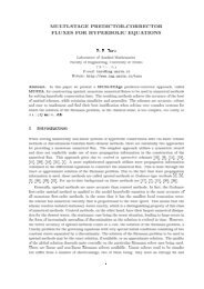
<strong>in</strong>tercept we use <strong>the</strong> value 0.001. Figure 1 illustrates <strong>the</strong> dependence <strong>of</strong> <strong>the</strong> optimal<br />
weight w∗ and <strong>the</strong> rescaled variance parameter ρ = d2/(1 + d2), which mimics <strong>in</strong><br />
a way <strong>the</strong> <strong>in</strong>traclass correlation and has <strong>the</strong> advantage to be bounded such that <strong>the</strong><br />
whole range <strong>of</strong> slope variances d2 can be shown. The optimal weight <strong>for</strong> <strong>the</strong> prediction<br />
<strong>of</strong> <strong>in</strong>dividual parameters <strong>in</strong>creases <strong>in</strong> <strong>the</strong> slope variance d2 from 0.5 <strong>for</strong> d2 → 0<br />
to about 0.91 <strong>for</strong> d2 → ∞. For d1 < 1/m <strong>the</strong> Bayesian optimal design, which is also<br />
optimal <strong>for</strong> <strong>the</strong> prediction <strong>of</strong> <strong>in</strong>dividual deviations, has optimal weight w∗ = 1 <strong>for</strong><br />
all positive values <strong>of</strong> d2, which results <strong>in</strong> a s<strong>in</strong>gular design.<br />
In Figure 2 <strong>the</strong> efficiencies eff(ξ ) = Φ(ξw∗)/Φ(ξ ) are plotted <strong>for</strong> <strong>the</strong> optimal<br />
design ξ0.5 <strong>in</strong> <strong>the</strong> fixed effects model ignor<strong>in</strong>g <strong>the</strong> <strong>in</strong>dividual effects and<br />
<strong>for</strong> <strong>the</strong> naive equidistant design ¯ ξ , which assigns weights 1/m to <strong>the</strong> m sett<strong>in</strong>gs<br />
x j = ( j − 1)/(m − 1). For <strong>the</strong> prediction <strong>of</strong> <strong>in</strong>dividual parameters <strong>the</strong> efficiency <strong>of</strong><br />
<strong>the</strong> design ξ0.5 decreases from 1 <strong>for</strong> d2 → 0 to approximately 0.60 <strong>for</strong> d2 → ∞,<br />
whereas ¯ ξ shows an overall lower per<strong>for</strong>mance go<strong>in</strong>g down to 0.42 <strong>for</strong> large d2.<br />
For <strong>the</strong> prediction <strong>of</strong> <strong>in</strong>dividual deviations <strong>the</strong> efficiency <strong>of</strong> both designs show a<br />
bathtub shaped behavior with limit<strong>in</strong>g efficiency <strong>of</strong> 1 <strong>for</strong> d2 → 0 or d2 → ∞. This<br />
is due to <strong>the</strong> fact that all regular designs are equally good <strong>for</strong> small d2 and equally<br />
bad <strong>for</strong> large d2, s<strong>in</strong>ce <strong>the</strong> criterion function (15) behaves like tr(∆V) <strong>for</strong> d2 → ∞<br />
<strong>in</strong>dependently <strong>of</strong> ξ . The m<strong>in</strong>imal efficiencies are 0.57 <strong>for</strong> ξ0.5 and 0.43 <strong>for</strong> ¯ ξ .<br />
For <strong>the</strong> sake <strong>of</strong> completeness also <strong>the</strong> efficiency is plotted with respect to <strong>the</strong><br />
Bayes criterion, which equals <strong>the</strong> first term <strong>in</strong> both criteria (12) and (15) to show<br />
that <strong>the</strong> efficiency may differ although <strong>the</strong> design optimization seems to be <strong>the</strong> same.<br />
This difference is due to <strong>the</strong> second (constant) term <strong>in</strong> (15). It should also be noted
<strong>Optimal</strong> <strong>Designs</strong> <strong>for</strong> <strong>Prediction</strong> <strong>of</strong> <strong>Individual</strong> <strong>Effects</strong> 7<br />
w*<br />
1.0<br />
0.8<br />
0.6<br />
0.4<br />
0.2<br />
0.0<br />
0.0 0.2 0.4 0.6 0.8 1.0<br />
Fig. 1 <strong>Optimal</strong> weights w ∗ <strong>for</strong> <strong>the</strong> prediction <strong>of</strong> <strong>in</strong>dividual parameters (solid l<strong>in</strong>e) and <strong>for</strong> <strong>the</strong><br />
prediction <strong>of</strong> <strong>in</strong>dividual deviations (dashed l<strong>in</strong>e)<br />
that <strong>the</strong> present efficiencies cannot be <strong>in</strong>terpreted as sav<strong>in</strong>gs or additional needs <strong>in</strong><br />
terms <strong>of</strong> sample sizes as <strong>in</strong> fixed effect models.<br />
5 Discussion and conclusions<br />
In this paper we po<strong>in</strong>t out similarities and differences <strong>in</strong> <strong>the</strong> <strong>the</strong>ory <strong>of</strong> optimal designs<br />
<strong>for</strong> <strong>the</strong> prediction <strong>of</strong> <strong>in</strong>dividual parameters and <strong>in</strong>dividual deviations compared<br />
to Bayesian designs. The objective function <strong>of</strong> <strong>the</strong> IMSE-criterion is a weighted av-<br />
eff<br />
1.0<br />
0.8<br />
0.6<br />
0.4<br />
0.2<br />
0.0<br />
0.0 0.2 0.4 0.6 0.8 1.0<br />
ρ<br />
ρ<br />
eff<br />
0.0 0.2 0.4 0.6 0.8 1.0<br />
Fig. 2 Efficiency <strong>of</strong> ξ0.5 (left panel) and ¯ ξ (right panel) <strong>for</strong> <strong>the</strong> prediction <strong>of</strong> <strong>in</strong>dividual parameters<br />
(solid l<strong>in</strong>e), <strong>in</strong>dividual deviations (dashed l<strong>in</strong>e) and <strong>the</strong> Bayes criterion (dotted l<strong>in</strong>e)<br />
1.0<br />
0.8<br />
0.6<br />
0.4<br />
0.2<br />
0.0<br />
ρ
8 Maryna Prus and Ra<strong>in</strong>er Schwabe<br />
erage <strong>of</strong> <strong>the</strong> Bayesian and <strong>the</strong> “standard” counterparts <strong>in</strong> <strong>the</strong> case <strong>of</strong> prediction <strong>of</strong><br />
<strong>in</strong>dividual parameters and def<strong>in</strong>es, hence, a compound criterion. For <strong>the</strong> prediction<br />
<strong>of</strong> <strong>in</strong>dividual deviations <strong>the</strong> Bayesian optimal designs rema<strong>in</strong> optimal, while <strong>the</strong><br />
criteria differ by an additive constant.<br />
A generalization <strong>of</strong> <strong>the</strong> present results to s<strong>in</strong>gular dispersion matrices D is<br />
straight<strong>for</strong>ward, although <strong>the</strong>re is no Bayesian counterpart <strong>in</strong> that case and <strong>the</strong> <strong>for</strong>mulae<br />
become less appeal<strong>in</strong>g. Such s<strong>in</strong>gular dispersion matrices naturally occur, if<br />
only parts <strong>of</strong> <strong>the</strong> parameter vector are random and <strong>the</strong> rema<strong>in</strong><strong>in</strong>g l<strong>in</strong>ear comb<strong>in</strong>ations<br />
are constant across <strong>the</strong> population. In particular, <strong>in</strong> <strong>the</strong> case <strong>of</strong> a random <strong>in</strong>tercept<br />
model, when all o<strong>the</strong>r parameters are fixed, <strong>the</strong> optimal design <strong>for</strong> <strong>the</strong> prediction <strong>of</strong><br />
<strong>the</strong> <strong>in</strong>dividual parameters can be obta<strong>in</strong>ed as <strong>the</strong> optimal one <strong>in</strong> <strong>the</strong> correspond<strong>in</strong>g<br />
model without <strong>in</strong>dividual effects (Prus and Schwabe, 2011), while <strong>for</strong> prediction <strong>of</strong><br />
<strong>the</strong> <strong>in</strong>dividual deviations any mean<strong>in</strong>gful design will be optimal.<br />
The method proposed may be directly extended to o<strong>the</strong>r l<strong>in</strong>ear design criteria<br />
as well as to <strong>the</strong> class <strong>of</strong> Φq-criteria based on <strong>the</strong> eigenvalues <strong>of</strong> <strong>the</strong> mean squared<br />
error matrix. Although <strong>the</strong> design optimality presented here is <strong>for</strong>mulated <strong>for</strong> approximate<br />
designs, which generally may not be exactly realized. These optimal approximate<br />
designs can serve as a benchmark <strong>for</strong> candidates <strong>of</strong> exact designs, which<br />
<strong>for</strong> example are obta<strong>in</strong>ed by appropriate round<strong>in</strong>g <strong>of</strong> <strong>the</strong> optimal weights. <strong>Optimal</strong><br />
designs <strong>for</strong> situations, which allows <strong>for</strong> different <strong>in</strong>dividual designs, will be subject<br />
<strong>of</strong> future research, <strong>in</strong> particular, <strong>in</strong> <strong>the</strong> case <strong>of</strong> sparse sampl<strong>in</strong>g, where <strong>the</strong> number<br />
<strong>of</strong> observations per <strong>in</strong>dividual is less than <strong>the</strong> number <strong>of</strong> parameters.<br />
Acknowledgements This research was partially supported by grant SKAVOE 03SCPAB3 <strong>of</strong> <strong>the</strong><br />
German Federal M<strong>in</strong>istry <strong>of</strong> Education and Research (BMBF). Part <strong>of</strong> <strong>the</strong> work was done dur<strong>in</strong>g a<br />
visit at <strong>the</strong> International Newton Institute <strong>in</strong> Cambridge.<br />
References<br />
1. Fedorov, V., Hackl, P.: Model-Oriented Design <strong>of</strong> Experiments. Spr<strong>in</strong>ger, New York (1997)<br />
2. Gladitz, J., Pilz, J.: Construction <strong>of</strong> optimal designs <strong>in</strong> random coefficient regression models.<br />
Statistics 13, 371–385 (1982)<br />
3. Henderson, C. R.: Best l<strong>in</strong>ear unbiased estimation and prediction under a selection model.<br />
Biometrics 31, 423–477 (1975)<br />
4. Kiefer, J.: General equivalence <strong>the</strong>ory <strong>for</strong> optimum designs (approximate <strong>the</strong>ory). Annals <strong>of</strong><br />
Statistics 2, 849–879 (1974)<br />
5. Prus, M., Schwabe, R.: <strong>Optimal</strong> <strong>Designs</strong> <strong>for</strong> <strong>Individual</strong> <strong>Prediction</strong> <strong>in</strong> <strong>Random</strong> Coefficient<br />
Regression Models. In: V. Melas, G. Nachtmann and D. Rasch (Eds.): <strong>Optimal</strong> Design <strong>of</strong><br />
Experiments - Theory and Application: Proceed<strong>in</strong>gs <strong>of</strong> <strong>the</strong> International Conference <strong>in</strong> Honor<br />
<strong>of</strong> <strong>the</strong> late Jagdish Srivastava, pp. 122–129. Center <strong>of</strong> Experimental Design, University <strong>of</strong><br />
Natural Resources and Life Sciences, Vienna (2011)<br />
6. Silvey, S. D.: <strong>Optimal</strong> Design. Chapman & Hall, London (1980)