Finite volume transport schemes for Voronoi meshes
Finite volume transport schemes for Voronoi meshes
Finite volume transport schemes for Voronoi meshes

You also want an ePaper? Increase the reach of your titles
YUMPU automatically turns print PDFs into web optimized ePapers that Google loves.
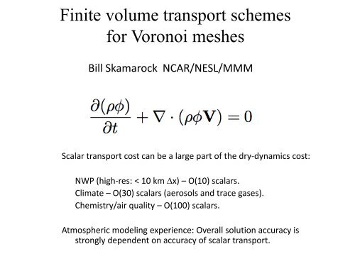
<strong>Finite</strong> <strong>volume</strong> <strong>transport</strong> <strong>schemes</strong><br />
<strong>for</strong> <strong>Voronoi</strong> <strong>meshes</strong><br />
Bill Skamarock NCAR/NESL/MMM<br />
Scalar <strong>transport</strong> cost can be a large part of the dry-dynamics cost:<br />
NWP (high-res: < 10 km Dx) – O(10) scalars.<br />
Climate – O(30) scalars (aerosols and trace gases).<br />
Chemistry/air quality – O(100) scalars.<br />
Atmospheric modeling experience: Overall solution accuracy is<br />
strongly dependent on accuracy of scalar <strong>transport</strong>.
Conservation of mass<br />
(conservative, flux <strong>for</strong>m)<br />
Conservation of scalar mass<br />
(conservative, flux <strong>for</strong>m)<br />
<strong>Finite</strong>-<strong>volume</strong> <strong>for</strong>mulation:<br />
Integrating in space and time<br />
over a fixed <strong>volume</strong>,<br />
use the divergence theorem<br />
where f is a dimensionless mixing ratio<br />
Consider two <strong>for</strong>mulations – (1)<br />
Scheme: approximate space-time integral of flux through cell surface
Consider two <strong>for</strong>mulations – (2)<br />
<strong>Finite</strong>-<strong>volume</strong> <strong>for</strong>mulation:<br />
Integrating in space over a<br />
fixed <strong>volume</strong>, use the<br />
divergence theorem<br />
Scheme: instantaneous integral of flux through cell surface, ODE (time)
MPAS (<strong>Voronoi</strong> mesh): Formulation (2)<br />
Instantaneous<br />
flux divergence in<br />
RK-based scheme
MPAS (<strong>Voronoi</strong> mesh): Formulation (2)<br />
Computing the flux - consider 1D <strong>transport</strong> (e.g. from WRF)<br />
2nd-order flux:<br />
3rd and 4th-order fluxes: (Hundsdorfer et al, JCP 1995; van Leer, 1985)<br />
where
MPAS (<strong>Voronoi</strong> mesh): Formulation (2)<br />
Recognizing<br />
We recast the 3rd and 4th order flux<br />
<strong>for</strong> the hexagonal grid as<br />
where x is the direction normal to the cell edge and i and i+1 are cell centers.<br />
We use the least-squares-fit polynomial to compute the second derivatives.
MPAS (<strong>Voronoi</strong> mesh): Formulation (2)<br />
Edge e 1 has weights <strong>for</strong><br />
computing second derivatives at<br />
cell centers C 0 and C 1.<br />
The weights <strong>for</strong> C 0 apply to cell<br />
centers C 0 through C 6, and the<br />
weights <strong>for</strong> C 1 apply to cell<br />
centers C 0-C 2 and C 6-C 9.
MPAS (<strong>Voronoi</strong> mesh): Formulation (2)
MPAS (<strong>Voronoi</strong> mesh): Formulation (2)<br />
Day 9 solution,<br />
Jablonowski and Williamson (2006)<br />
baroclinic wave test case<br />
10242 cell (240 km) mesh solution errors
MPAS (<strong>Voronoi</strong> mesh): Formulation (1)<br />
<strong>Finite</strong>-<strong>volume</strong> <strong>for</strong>mulation:<br />
Integrating in space and time<br />
over a fixed <strong>volume</strong>,<br />
use the divergence theorem<br />
Scheme: approximate space-time integral of flux through cell surface
MPAS (<strong>Voronoi</strong> mesh): Formulation (1)
MPAS (<strong>Voronoi</strong> mesh): Formulation (1)<br />
M07 and LR05 used first-order reconstructions<br />
Lashley and Thuburn (2002) and<br />
Skamarock and Menchaca (2010)<br />
use second and fourth-order reconstructions, e.g.<br />
The least-squares polynomial fit is constrained to pass through the cell-center value<br />
by fitting a polynomial of the <strong>for</strong>m<br />
The constant (c 0 = � 0) is adjusted such that the cell-integrated polynomial is equal<br />
to the cell-average value times the cell area.
MPAS (<strong>Voronoi</strong> mesh): Formulations (1) and (2)<br />
Blossey and Durran<br />
de<strong>for</strong>mational flow<br />
test case
MPAS (<strong>Voronoi</strong> mesh): Formulation (1*)<br />
(1) Fit quadratic polynomial to cell<br />
center and cell vertex values<br />
(2) Cell-vertex values are a weighted<br />
sum of nearest and next-nearest cells
MPAS (<strong>Voronoi</strong> mesh): Formulation (1*)<br />
(3) Polynomial constraints<br />
(2) Cell-vertex values<br />
Perfect hexagons: = 3<br />
2<br />
This leads to a 4 th order accurate<br />
gradient operator on perfect hexagons<br />
1<br />
2
MPAS (<strong>Voronoi</strong> mesh): Formulations (1*) and (2)
MPAS (<strong>Voronoi</strong> mesh): Formulations (1) and (1*)<br />
Solid body rotation, slotted cylinder
MPAS (<strong>Voronoi</strong> mesh): Formulations (2) and (1*)<br />
Slotted cylinder de<strong>for</strong>mational flow test case<br />
Lauritzen et al (2012)<br />
Miura and Skamarock (2012)<br />
<strong>for</strong>mulation (1*)<br />
FCT limiter<br />
T/2 T<br />
Skamarock and Gassmann (2011)<br />
<strong>for</strong>mulation (2)<br />
FCT limiter<br />
Miura and Skamarock (2012); <strong>for</strong>mulation (1*)<br />
Skamarock and Gassmann (2011); <strong>for</strong>mulation (2)
MPAS (<strong>Voronoi</strong> mesh): Formulations (1*)<br />
Blossey and Durran de<strong>for</strong>mational flow test case<br />
Blossey and Durran<br />
de<strong>for</strong>mational flow<br />
test case<br />
Dx 60 km Dx 60 km, FCT lim Dx 120 km, FCT lim Dx 240 km, FCT lim
MPAS (<strong>Voronoi</strong> mesh): Formulations (1*)<br />
Blossey and Durran de<strong>for</strong>mational flow test case<br />
MS (2012) FIT limiter<br />
Dx = 120 km<br />
MS (2012) FIT<br />
(lower bnd only)<br />
Dx = 120 km<br />
MS (2012) FIT<br />
(lower bnd only)<br />
Dx = 60 km
<strong>Finite</strong> <strong>volume</strong> <strong>transport</strong> <strong>schemes</strong><br />
<strong>for</strong> <strong>Voronoi</strong> <strong>meshes</strong><br />
Summary<br />
We examined 3 newer <strong>schemes</strong> using 2+ order reconstructions or<br />
higher-order <strong>for</strong>mulations.<br />
The new <strong>schemes</strong> show significantly reduced phase and amplitude<br />
error relative to 1 st order reconstructions.<br />
Runge-Kutta-based scheme appears to be the most robust.<br />
While Miura and Skamarock (2012) scheme appears most accurate,<br />
some problematic behavior (non-convergence) appears when used with<br />
FCT-type limiters.<br />
Nonlinear limiters/renormalization – lessons learned?