ECE 316 – Probability Theory and Random Processes

Problems
ECE 316 – Probability Theory and Random Processes
Chapter 4 Solutions (Part 2)
Xinxin Fan
20. A gambling book recommends the following “winning strategy” for the game of roulette. It
recommends that a gambler bet $1 on red. If red appears (which has probability 18
38 ), then the
gambler should take her $1 profit and quit. If the gambler loses this bet (which has probability
20
38 of occurring), she should make additional $1 bets on red on each of the next two spins of
the roulette wheel and then quit. Let X denote the gambler’s winnings when she quits.
(a) Find P {X > 0}.
(b) Are you convinced that the strategy is indeed a “winning” strategy? Explain your answer!
(c) Find E[X].
Solution. (a) The event that X > 0 denotes that the gambler wins the first bet or he loses
the first bet and wins the next two bets. Therefore, we get
P {X > 0} = P {win first bet} + P {lose, win, win} = 18 20
+
38 38 ·
� �2 18
≈ 0.5981.
38
(b) The strategy described above is not a “winning” strategy because if the gambler wins
then he or she wins $1. However, a loss would either be $1 or $3.
(c) We first note that the random variable X can take on 1, −1 and −3, where “–” denotes
that the gambler loses money. Then we obtain
P {X = 1} = P {win first bet} + P {lose, win, win} = 18 20
+
38 38 ·
� �2 18
,
38
P {X = −1} = P {lose, lose, win} + P {lose, win, lose} = 2 · 18
38 ·
� �2 20
,
38
� �3 20
P {X = −3} = P {lose, lose, lose} = .
38
Therefore, we can compute the expectation as follows:
E[X] = 1 · P {X = 1} + (−1) · P {X = −1} + (−3) · P {X = −3} ≈ −0.108.
25. A typical slot machine has 3 dials, each with 20 symbols (cherries, lemons, plums, oranges,
bells, and bars). A typical set of dials is shown in Table 1. According to this table, of the
20 slots on dial 1, 7 are cherries, 3 are oranges, and so on. A typical payoff on a 1-unit
1

Table 1: Slot machine dial setup
Dial 1 Dial 2 Dial 3
Cherries 7 7 0
Oranges 3 7 6
Lemons 3 0 4
Plums 4 1 6
Bells 2 2 3
Bars 1 3 1
20 20 20
Table 2: Typical payoff on a 1-unit bet
Dial 1 Dial 2 Dial 3 Payoff
Bar Bar Bar 60
Bell Bell Bell 20
Bell Bell Bar 18
Plum Plum Plum 14
Orange Orange Orange 10
Orange Orange Bar 8
Cherry Cherry Anything 2
Cherry No cherry Anything 0
Anything else -1
bet is shown in Table 2. Compute the player’s expected winnings on a single play of the slot
machine. Assume that each dial acts independently.
Solution. Let X denote the payoff on a 1-unit bet. Then we get
P {X = 60} = P {Bar, Bar, Bar} = 1 3 1 3
· · =
20 20 20 8000 ,
P {X = 20} = P {Bell, Bell, Bell} = 2 2 3 12
· · =
20 20 20 8000 ,
P {X = 18} = P {Bell, Bell, Bar} = 2 2 1 4
· · =
20 20 20 8000 ,
P {X = 14} = P {Plum, Plum, Plum} = 4 1 6 24
· · =
20 20 20 8000 ,
P {X = 10} = P {Orange, Orange, Orange} = 3 7 6 126
· · =
20 20 20 8000 ,
P {X = 8} = P {Orange, Orange, Bar} = 3 7 1 21
· · =
20 20 20 8000 ,
P {X = 2} = P {Cherry, Cherry, Anything} = 7 7 49
· =
20 20 400 ,
2

P {X = 0} = P {Cherry, No cherry, Anything} = 7 13 91
· =
20 20 400 ,
P {X = −1} =
3 + 12 + 4 + 24 + 126 + 21 + 980 + 1820
P {Anything else} = 1 −
8000
= 501
800 .
Therefore, the player’s expected winnings on a single play of the slot machine can be computed
as follows:
E[X] = 60 · P {X = 60} + 20 · P {X = 20} + 18 · P {X = 18} +
= 180 + 240 + 72 + 336 + 1260 + 168 + 1960 − 5010
14 · P {X = 14} + 10 · P {X = 10} + 8 · P {X = 8} +
2 · P {X = 2} + 0 · P {X = 0} + (−1) · P {X = −1}
= −0.09925.
8000
32. To determine whether or not they have a certain disease, 100 people are to have their blood
tested. However, rather than testing each individual separately, it has been decided first to
group the people in groups of 10. The blood samples of the 10 people in each group will be
pooled and analyzed together. If the test is negative, one test will suffice for the 10 people;
whereas, if the test is positive each of the 10 people will also be individually tested and, in
all, 11 tests will be made on this group. Assume the probability that a person has the disease
is 0.1 for all people, independently of each other, and compute the expected number of tests
necessary for each group. (Note that we are assuming that the pooled test will be positive if
at least one person in the pool has the disease.)
Solution. Let T be the number of tests for a group of 10 people. Then we know that T = 1
if the test is negative and T = 11 if the test is positive. Therefore, we get
E[T ] = (0.9) 10 + 11[1 − (0.9) 10 ] = 11 − 10 · (0.9) 10 .
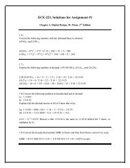
33. A newsboy purchases papers at 10 cents and sells them at 15 cents. However, he is not allowed
to return unsold papers. If his daily demand is a binomial random variable with n = 10, p = 1
3 ,
approximately how many papers should he purchase so as to maximize his expected profit?
Solution. Let a be the number of papers the newsboy purchases, X be the daily demand,
and Y be the profit the newsboy gets. Then we obtain the relation between random variables
X and Y as follows:
Y =
� 5a X ≥ a
15X − 10a X < a .
Therefore, the expected profit that the newsboy obtains is
E[Y ] = 5a · P (X ≥ a) + (15X − 10a) · P (X < a)
=
10�
i=a
5a ·
� 10
i
� � 1
3
� i � 2
3
� 10−i
�a−1
+ (15i − 10a) ·
i=0
� 10
i
� � 1
3
�i � �10−i 2
3
To find the approximate value for a, we can use Matlab to draw the following figure to show
the relation between E[Y ] and a. From Fig. 1, we note that the newsboy should purchase 3
papers so as to maximize his expected profit.
3

38. If E[X] = 1 and Var(X) = 5, find
(a) E[(2 + X) 2 ];
(b) Var(4 + 3X).
E[Y]
10
0
−10
−20
−30
−40
−50
0 1 2 3 4 5
a
6 7 8 9 10
Figure 1: The Expected Profit E[Y ]
Solution. (a) E[(2 + X) 2 ] = Var(2 + X) + (E[2 + X]) 2 = Var(X) + 9 = 14.
(b) Var(4 + 3X) = 9 · Var(X) = 45.
44. A satellite system consists of n components and functions on any given day if at least k of
the n components function on that day. On a rainy day each of the components independently
functions with probability p1, whereas on a dry day they each independently function with
probability p2. If the probability of rain tomorrow is α, what is the probability that the satellite
system will function?
Solution. The probability that the satellite system will function can be computed as follows:
P (system functions) = P (rain)P (system functions | rain) + P (dry)P (system functions | dry)
n�
� �
n
= α · p
i
i 1(1 − p1) n−i n�
� �
n
+ (1 − α) · p
i
i 2(1 − p2) n−i .
i=k
48. It is known that diskettes produced by a certain company will be defective with probability 0.01,
independently of each other. The company sells the diskettes in packages of size 10 and offers
a money-back guarantee that at most 1 of the 10 diskettes in the package will be defective. If
someone buys 3 packages, what is the probability that he or she will return exactly 1 of them?
Solution. Let p be the probability that a package will be returned. The we obtain
p = 1 − (0.99) 10 − 10 · (0.99) 9 (0.01).
Therefore, if someone buys 3 packages then the probability they will return exactly 1 package
is 3p(1 − p) 2 .
49. When coin 1 is flipped, it lands heads with probability 0.4; when coin 2 is flipped, it lands
heads with probability 0.7. One of these coins is randomly chosen and flipped 10 times.
4
i=k

(a) What is the probability that exactly 7 of the 10 flips land on heads?
(b) Given that the first of these ten flips lands heads, what is the conditional probability that
exactly 7 of the 10 flips land on heads?.
Solution. (a) Note that one of two coins will be randomly chosen, we get
P (7 heads) = P (coin 1)P (7 heads | coin 1) + P (coin 2)P (7 heads | coin 2)
= 1
2 ·
� 10
7
�
· (0.4) 7 · (0.6) 3 + 1
2 ·
� 10
7
(b) We can compute the conditional probability as follows:
P (7 heads | 1st heads) =
Theoretical Exercises
=
�
· (0.7) 7 · (0.3) 3 .
�2 i=1 P (coin i)P (7 heads, 1st heads | coin i)
P (1st heads)
1
2 · � � 9
6 · (0.4) 7 · (0.6) 3 1 + 2 · � � 9
6 · (0.7) 7 · (0.3) 3
1
2
· 0.4 + 1
2
· 0.7
4. If X has distribution function F , what is the distribution function of e X .
Solution. Let G(x) be the distribution function of e X . Then we need to consider the
following two cases:
• When x ≤ 0, we get
• When x > 0, we obtain
G(x) = P {e X ≤ x} = 0.
G(x) = P {e X ≤ x} = P {X ≤ ln x} = F (ln x).
5. If X has distribution function F , what is the distribution function of the random variable
αX + β, where α and β are constants, α �= 0?
Solution. Let G(x) be the distribution function of e X . Then we need to consider the
following two cases:
• When α > 0, we get
• When α < 0, we obtain
G(x) = P {αX + β ≤ x} = P
G(x) = P {αX + β ≤ x} = P
�
X ≥
5
�
X ≤
�
x − β
α
�
x − β
= F
α
� x − β
α
�
.
� �
x − β
= 1 − lim F − h .
h→0 + α
.

8. Let X be such that
Find c �= 1 such that E[c X ] = 1.
P {X = 1} = p = 1 − P {X = −1}.
Solution. We have known the probability mass function of X: P {X = 1} = p and P {X =
−1} = 1 − p. Thus,
E[c X ] = c 1 · +c −1 · (1 − p).
Let E[c X ] = cp + 1−p
c
that E[c X ] = 1.
= 1, it follows that c = p
1−p
or 1. Therefore, except 1, c = p
1−p satisfies
9. Let X be a random variable having expected value µ and variance σ 2 . Find the expected value
and variance of Y = X−µ
σ .
Solution. Using the properties of expected value and variance, we get
E[Y ] =
� �
X − µ
E =
σ
1
Var(Y ) =
1
· E[X − µ] = · (E[X] − µ) = 0,
σ σ
� � � �2 X − µ 1
Var = · Var(X) =
σ σ
σ2
= 1.
σ2 13. Let X be a binomial random variable with parameters (n, p). What value of p maximizes
P {X = k}, k = 0, 1, . . . , n? This is an example of a statistical method used to estimate p
when a binomial (n, p) random variable is observed to equal k. If we assume that n is known,
then we estimate p by choosing that value of p that maximizes P {X = k}. This is known as
the the method of maximum likelihood estimation.
Solution. Note that when P {X = k} achieves the maximum value, log P {X = k} also gets
the maximum value. Therefore, we can first take logarithm and then determine the p that
maximizes log P {X = k}. More specifically, we first obtain
� �
n
log P {X = k} = log + k · log p + (n − k) · log(1 − p).
k
Then we can find p by computing the derivative as follows:
Therefore, p = k
n
∂
k n − k
log P {X = k} = −
∂p p 1 − p
maximizes P {X = k} for k = 0, 1, . . . , n.
6
= 0.